socioeconomic heterogeneity in model applications (schema) · socioeconomic heterogeneity in model...
TRANSCRIPT

Socioeconomic Heterogeneity in Model Applications (SCHEMA)
G. Kiesewetter, N.D. Rao, S. K.C., H. ValinM. Cantele, S. Pachauri, P. Sauer, W. Schoepp, M. Speringer
ENE, ESM, MAG, POP Programs
SAC Meeting - 20/21 April 2015
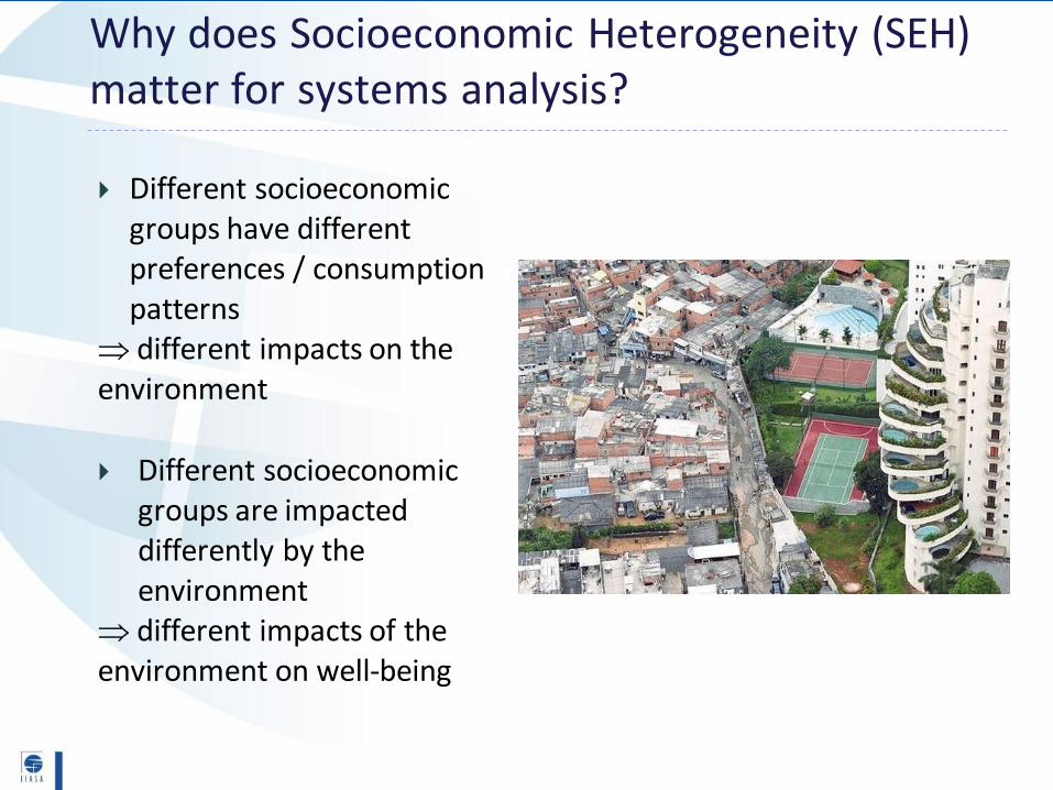
Different socioeconomic groups have different preferences / consumption patterns
different impacts on the environment
Different socioeconomic groups are impacted differently by the environment
different impacts of the environment on well-being
Why does Socioeconomic Heterogeneity (SEH) matter for systems analysis?
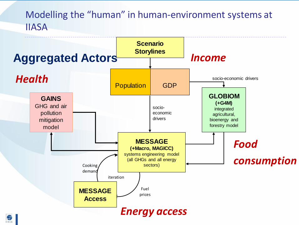
Modelling the “human” in human-environment systems at IIASA
Scenario
Storylines
Population GDP
GLOBIOM (+G4M)integrated
agricultural,
bioenergy and
forestry model
MESSAGE (+Macro, MAGICC)
systems engineering model
(all GHGs and all energy
sectors)
socio-economic drivers
Aggregated Actors
GAINSGHG and air
pollution
mitigation
model
Cooking
demand
iteration
MESSAGE
Access
Fuel
prices
socio-
economic
drivers
Health
Energy access
Food
consumption
Income
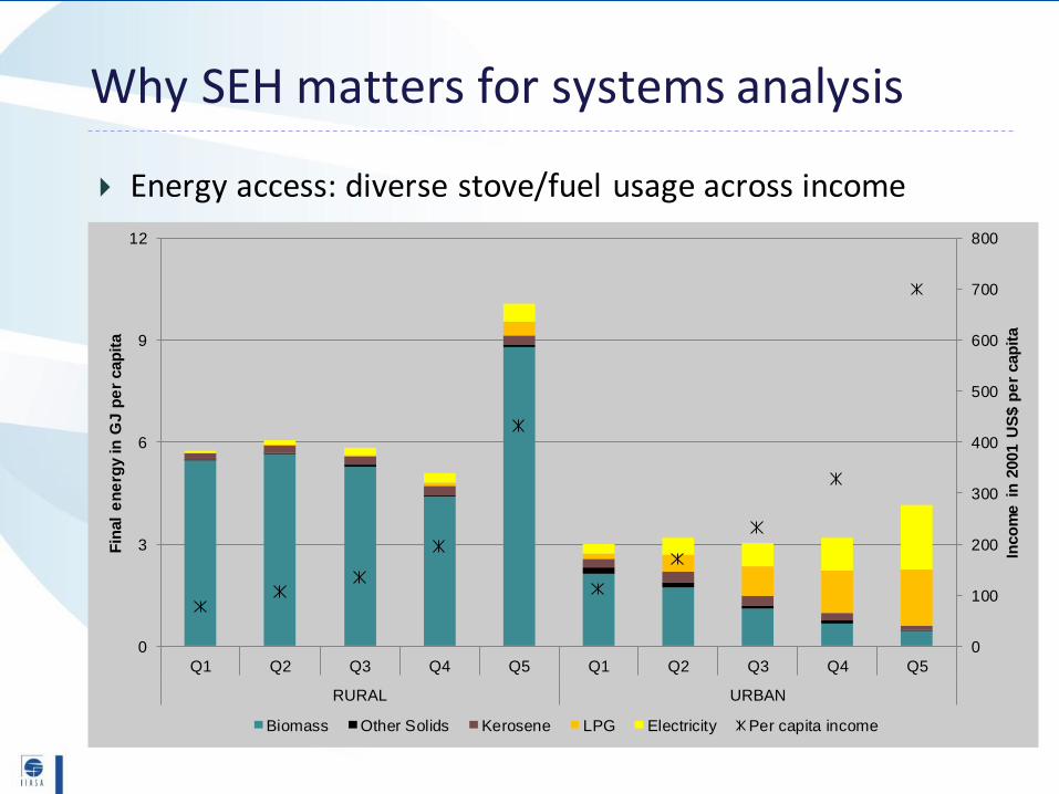
Why SEH matters for systems analysis
India, 2004-05
Energy access: diverse stove/fuel usage across income
groups
0
100
200
300
400
500
600
700
800
0
3
6
9
12
Q1 Q2 Q3 Q4 Q5 Q1 Q2 Q3 Q4 Q5
RURAL URBAN
Inco
me
in
2001 U
S$ p
er
cap
ita
Fin
al
en
erg
y in
GJ p
er
cap
ita
Biomass Other Solids Kerosene LPG Electricity Per capita income
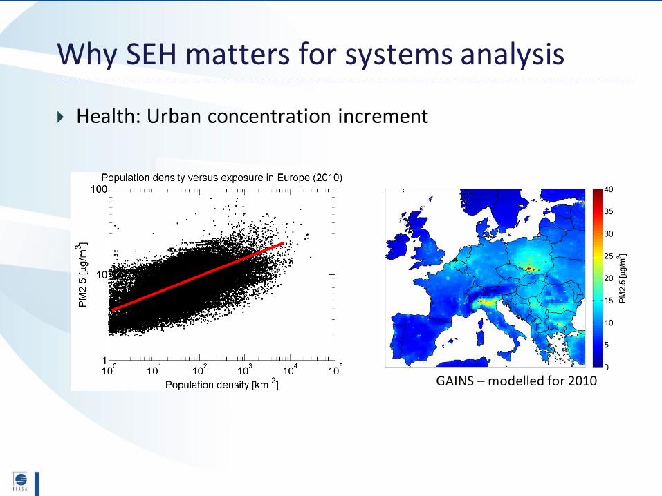
Health: Urban concentration increment
Why SEH matters for systems analysis
GAINS – modelled for 2010
Why SEH matters for systems analysis
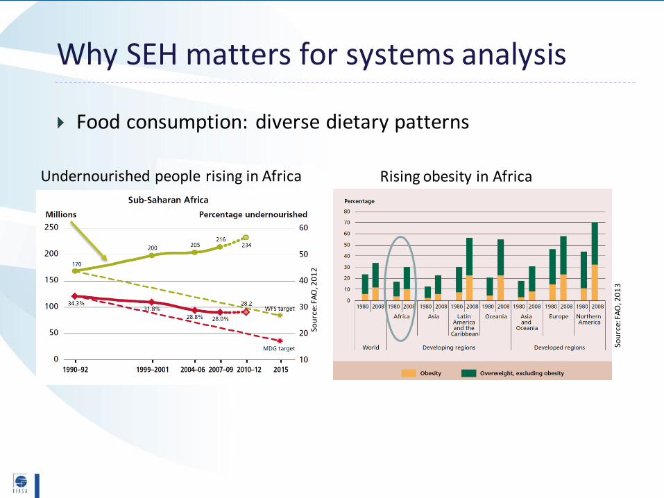
Food consumption: diverse dietary patterns
Undernourished people rising in Africa Rising obesity in Africa
Sou
rce:
FA
O, 2
01
3
Sou
rce:
FA
O, 2
01
2
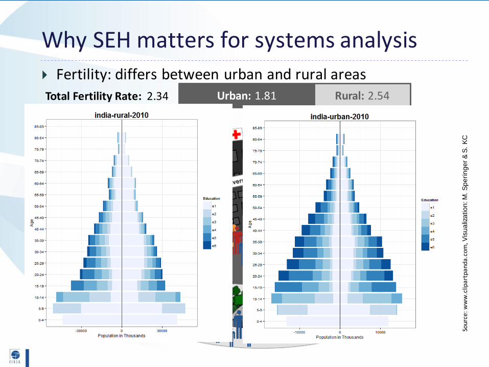
Why SEH matters for systems analysis
Fertility: differs between urban and rural areas
India
Sour
ce:
ww
w.c
lipar
tpan
da.c
om, V
isu
aliz
atio
n: M
. S
pe
rin
ge
r &
S.
KC
Urban: 1.81 Rural: 2.54Total Fertility Rate: 2.34
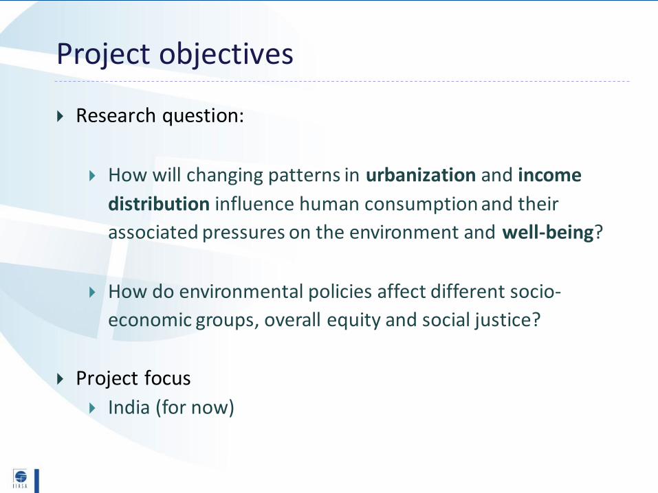
Project objectives
Research question:
How will changing patterns in urbanization and income
distribution influence human consumption and their
associated pressures on the environment and well-being?
How do environmental policies affect different socio-
economic groups, overall equity and social justice?
Project focus
India (for now)
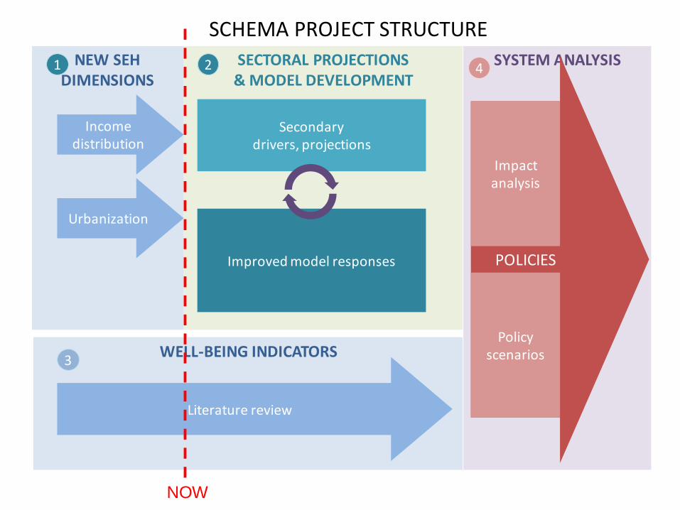
WELL-BEING INDICATORS
SECTORAL PROJECTIONS& MODEL DEVELOPMENT
SYSTEM ANALYSISNEW SEH DIMENSIONS
Literature review
POLICIES
Urbanization
Incomedistribution
Secondarydrivers, projections
Impact analysis
Policy scenarios
SCHEMA PROJECT STRUCTURE
1 2
5
3
4
Improved model responses
NOW
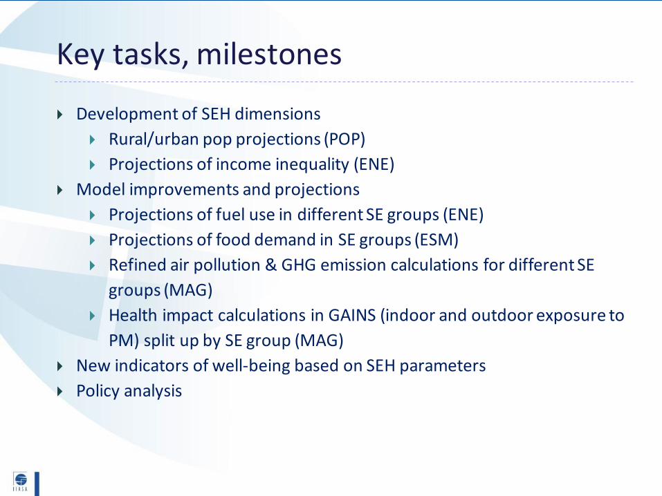
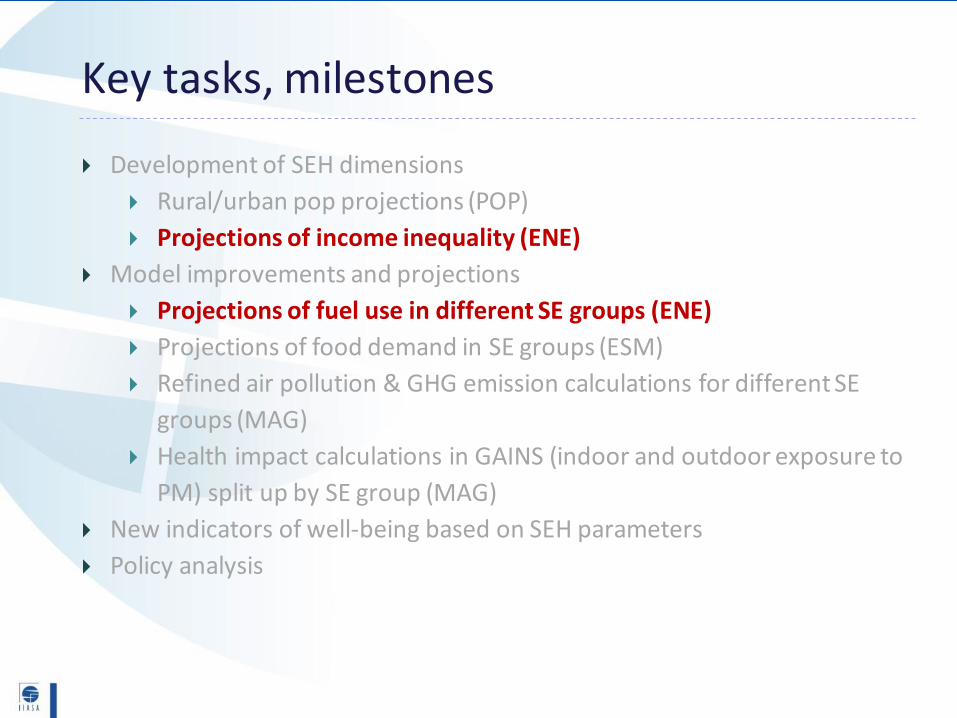
Key tasks, milestones
Development of SEH dimensions
Rural/urban pop projections (POP)
Projections of income inequality (ENE)
Model improvements and projections
Projections of fuel use in different SE groups (ENE)
Projections of food demand in SE groups (ESM)
Refined air pollution & GHG emission calculations for different SE
groups (MAG)
Health impact calculations in GAINS (indoor and outdoor exposure to
PM) split up by SE group (MAG)
New indicators of well-being based on SEH parameters
Policy analysis
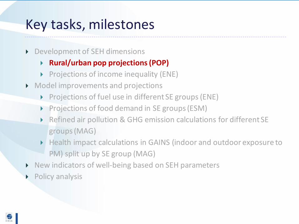
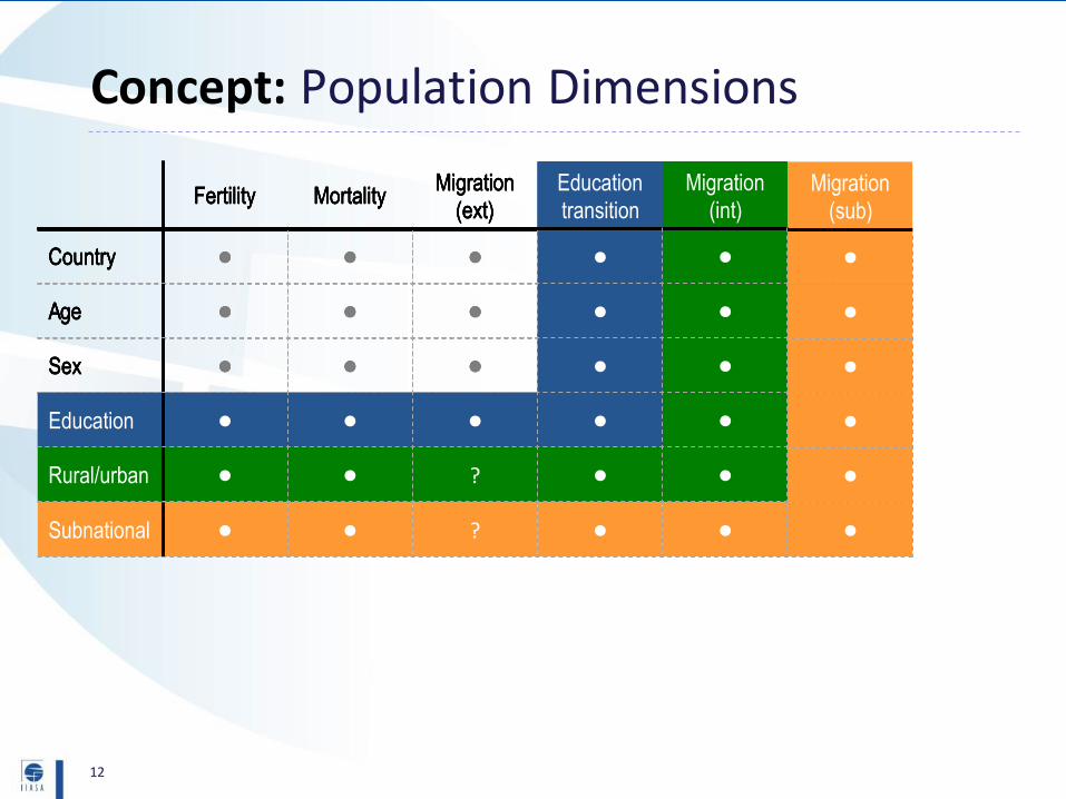
Concept: Population Dimensions
12
Fertility MortalityMigration
(ext)
Country • • •
Age • • •
Sex • • •
Fertility MortalityMigration
(ext)
Education
transition
Migration
(int)
Migration
(sub)
Country • • • • • •
Age • • • • • •
Sex • • • • • •
Education • • • • • •
Rural/urban • • ? • • •
Subnational • • ? • • •
Fertility MortalityMigration
(ext)
Education
transition
Migration
(int)
Country • • • • •
Age • • • • •
Sex • • • • •
Education • • • • •
Rural/urban • • ? • •
Fertility MortalityMigration
(ext)
Education
transition
Country • • • •
Age • • • •
Sex • • • •
Education • • • •
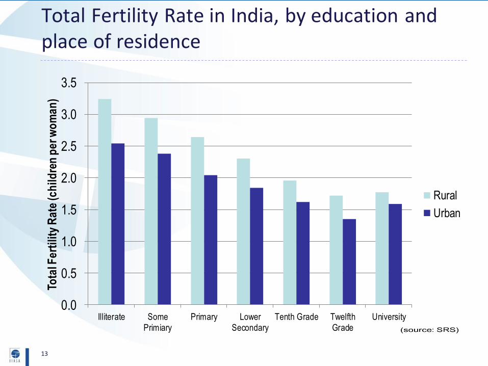
Total Fertility Rate in India, by education and place of residence
13
0.0
0.5
1.0
1.5
2.0
2.5
3.0
3.5
Illiterate Some
Primiary
Primary Lower
Secondary
Tenth Grade Twelfth
Grade
University
Tota
l Fe
rtil
ity
Ra
te (c
hil
dre
n p
er
wo
ma
n)
Rural
Urban
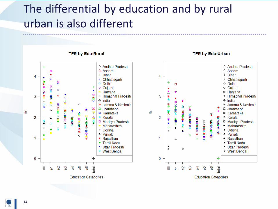
14
The differential by education and by rural urban is also different
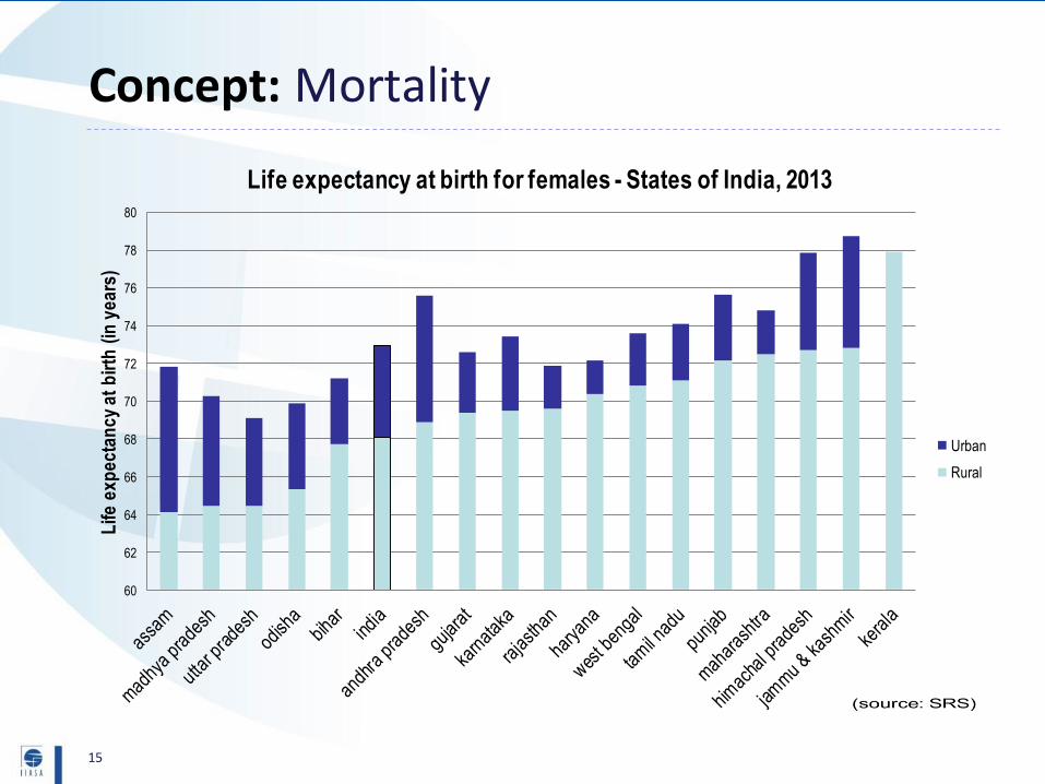
Concept: Mortality
15
60
62
64
66
68
70
72
74
76
78
80
Lif
e e
xp
ec
tan
cy
at
bir
th (
in y
ea
rs)
Life expectancy at birth for females - States of India, 2013
Urban
Rural
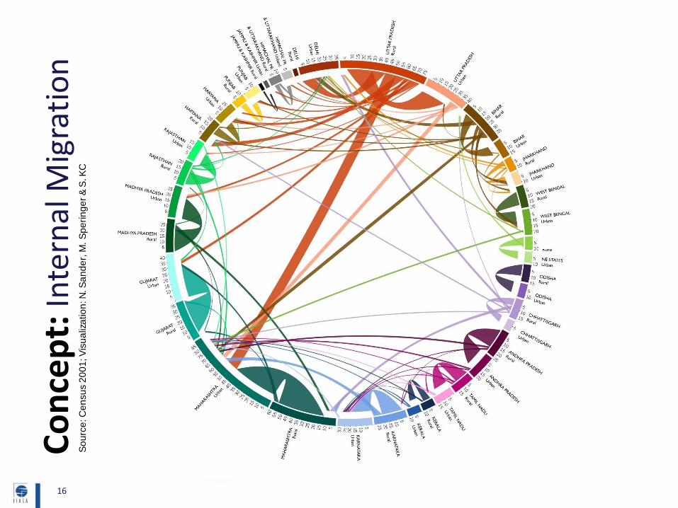
16
Co
nce
pt:
Inte
rnal
Mig
rati
on
So
urc
e: C
en
su
s 2
00
1; V
isu
aliz
atio
n: N
. S
an
de
r, M
. S
pe
rin
ge
r &
S. K
C
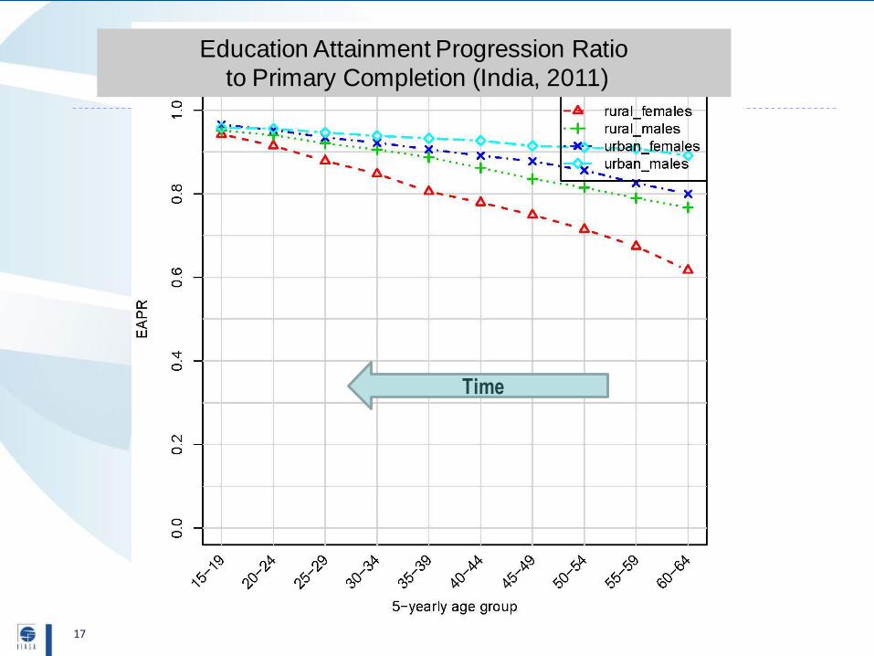
17
Education Attainment Progression Ratio
to Primary Completion (India, 2011)
Time
18
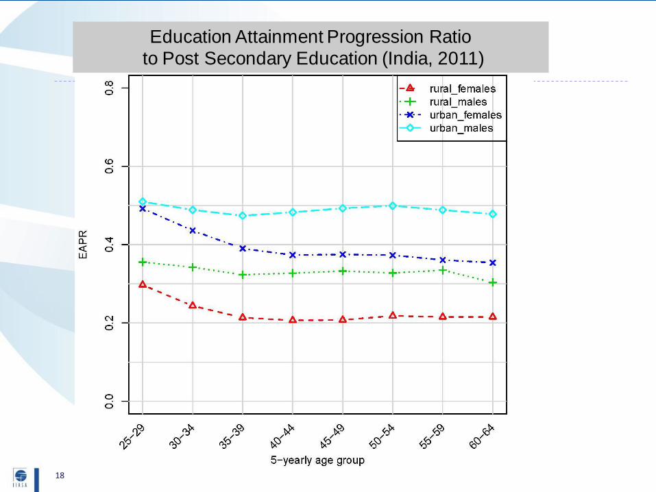
Education Attainment Progression Ratio
to Post Secondary Education (India, 2011)
19, date
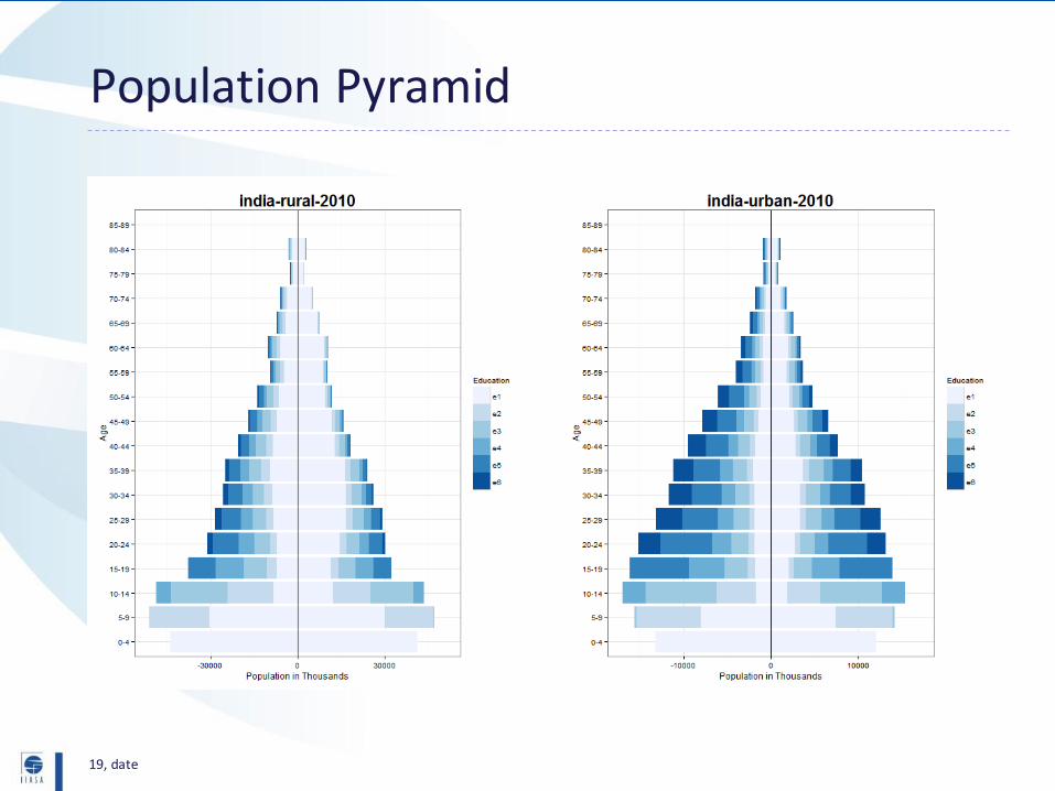
Population Pyramid
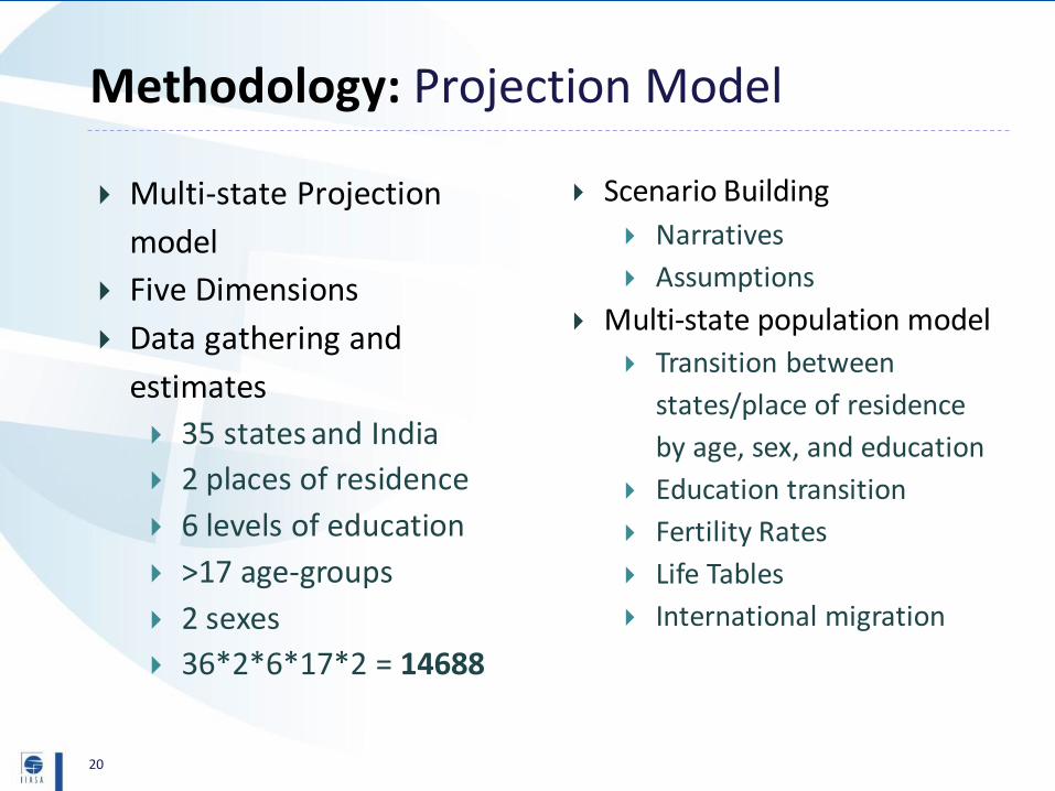
Multi-state Projection
model
Five Dimensions
Data gathering and
estimates
35 states and India
2 places of residence
6 levels of education
>17 age-groups
2 sexes
36*2*6*17*2 = 14688
Scenario Building
Narratives
Assumptions
Multi-state population model
Transition between
states/place of residence
by age, sex, and education
Education transition
Fertility Rates
Life Tables
International migration
20
Methodology: Projection Model
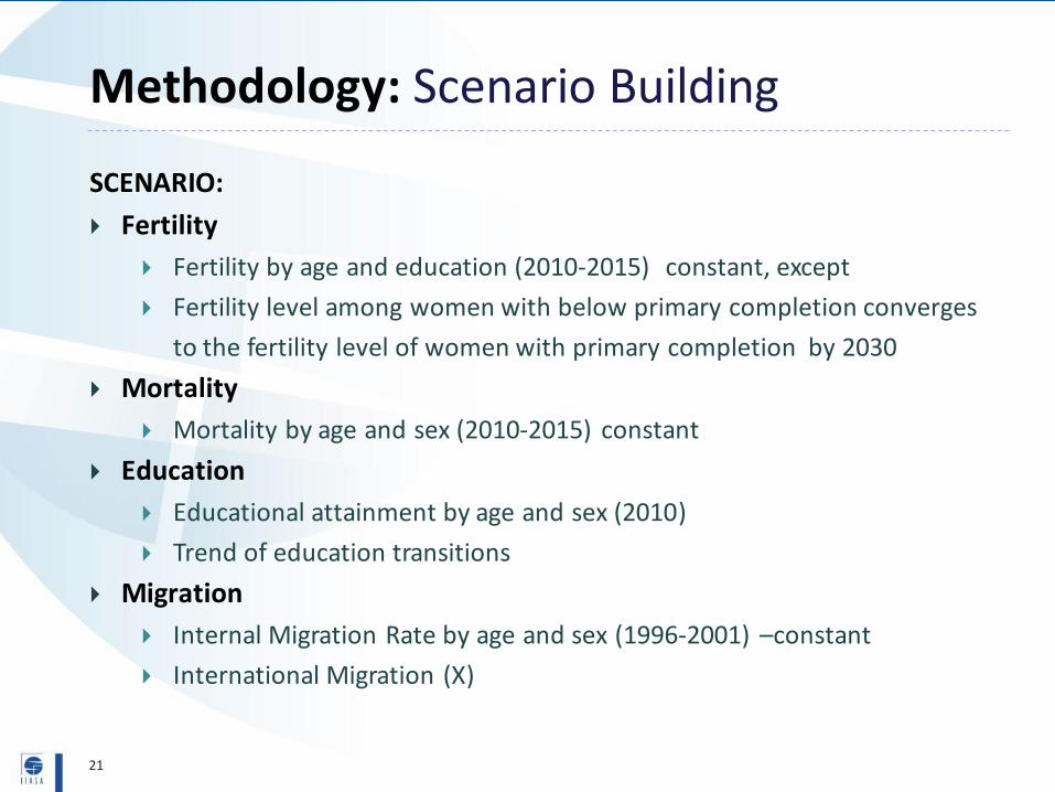
Methodology: Scenario Building
21
SCENARIO:
Fertility
Fertility by age and education (2010-2015) constant, except
Fertility level among women with below primary completion converges
to the fertility level of women with primary completion by 2030
Mortality
Mortality by age and sex (2010-2015) constant
Education
Educational attainment by age and sex (2010)
Trend of education transitions
Migration
Internal Migration Rate by age and sex (1996-2001) –constant
International Migration (X)
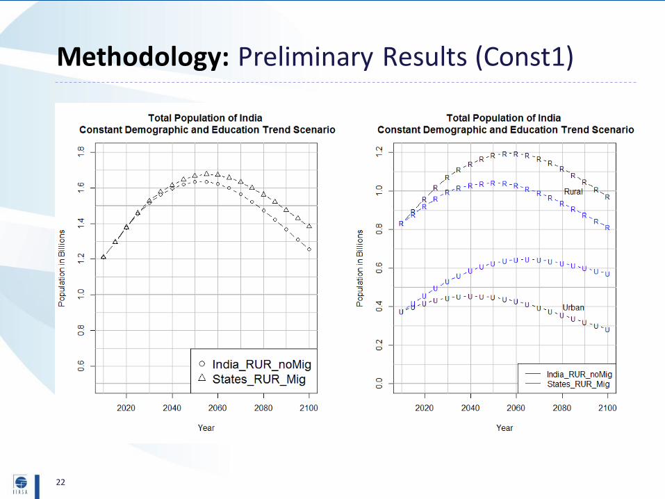
22
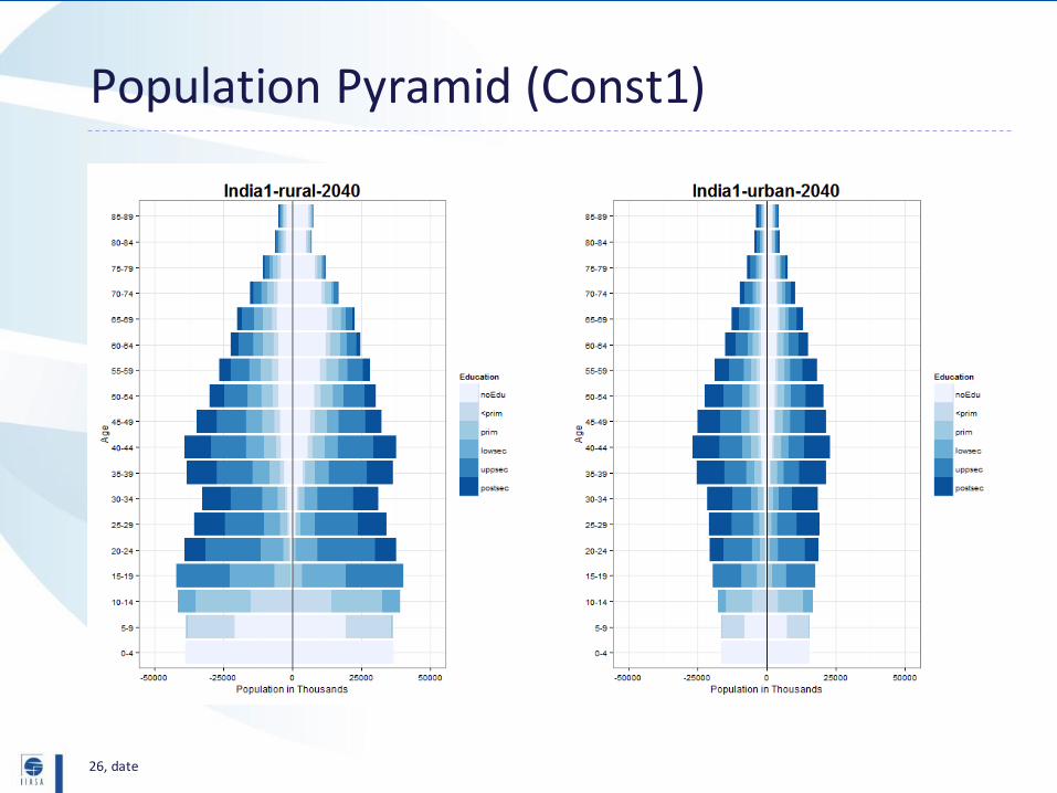
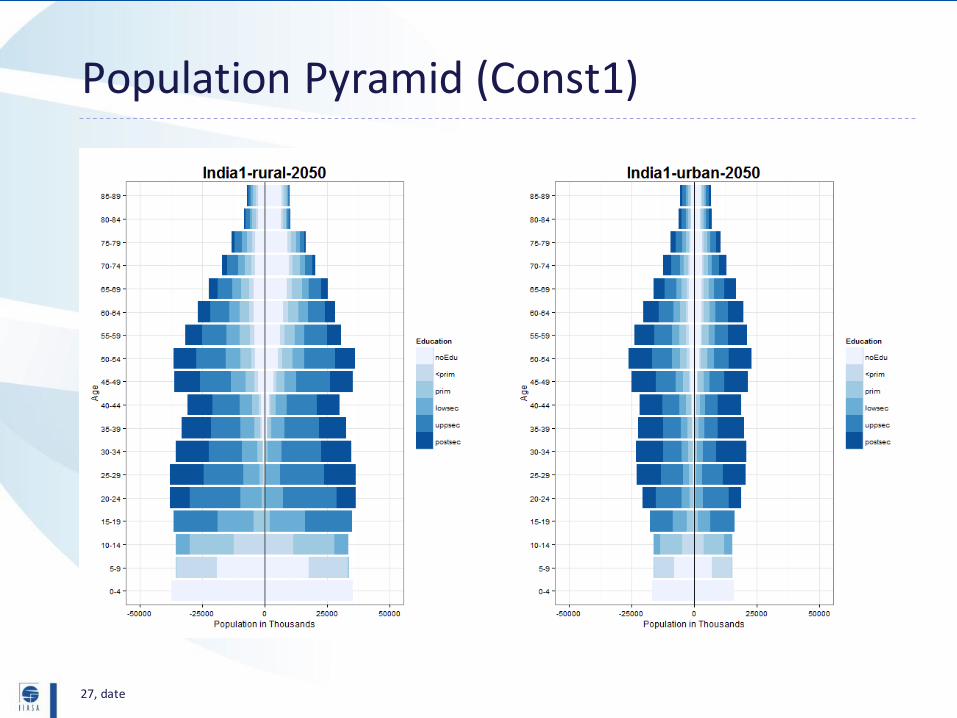
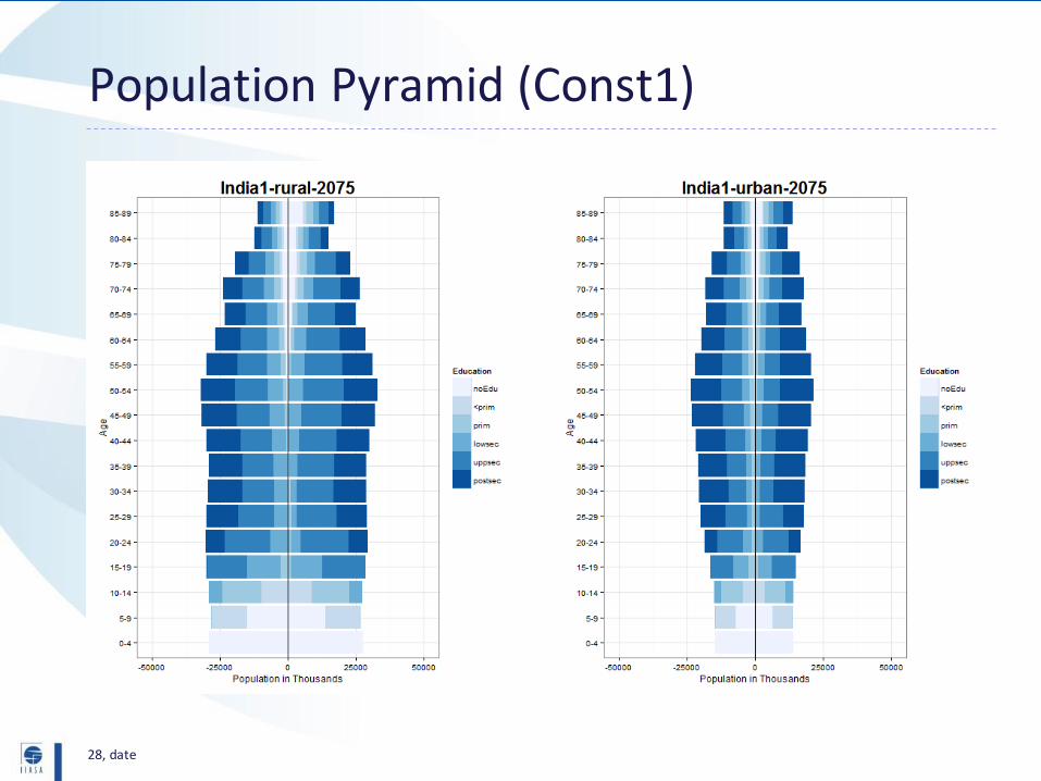
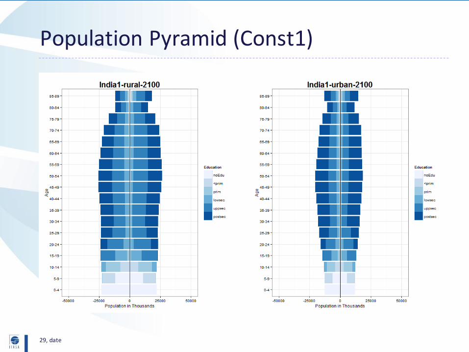
Methodology: Preliminary Results (Const1)
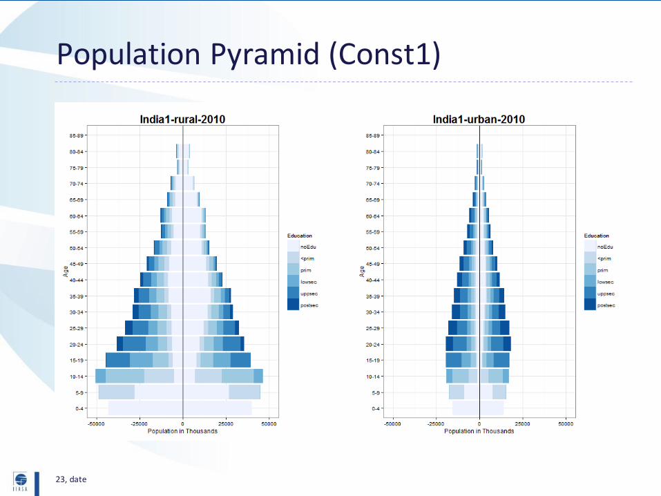
23, date
Population Pyramid (Const1)
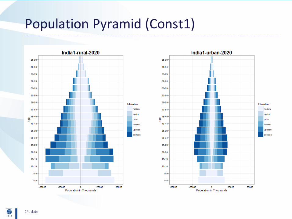
24, date
Population Pyramid (Const1)
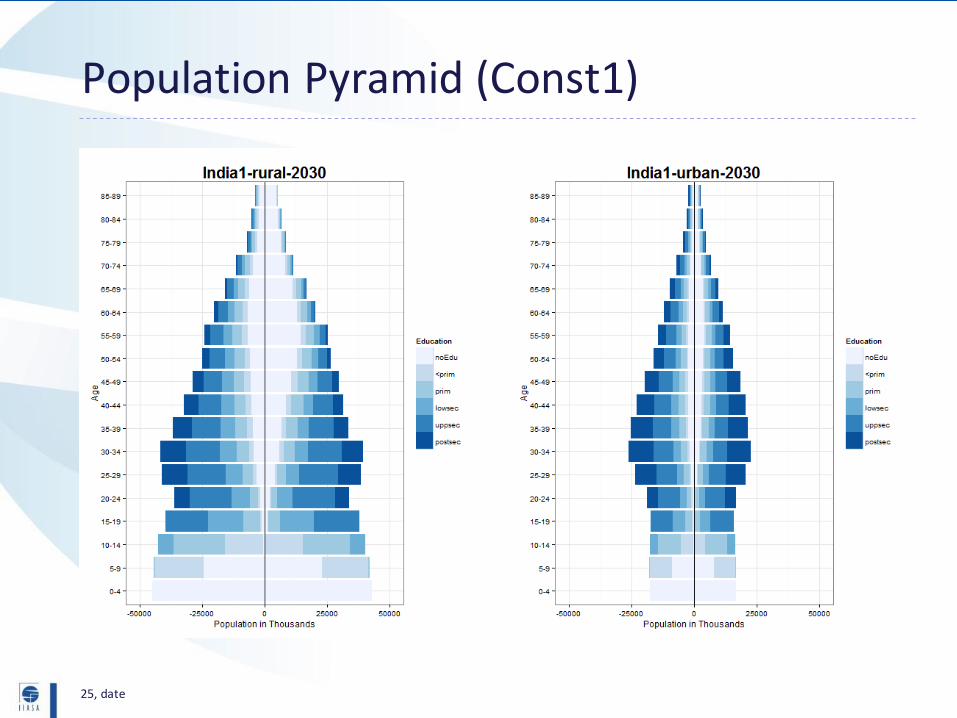
25, date
Population Pyramid (Const1)
26, date
Population Pyramid (Const1)
27, date
Population Pyramid (Const1)
28, date
Population Pyramid (Const1)
29, date
Population Pyramid (Const1)
Key tasks, milestones
Development of SEH dimensions
Rural/urban pop projections (POP)
Projections of income inequality (ENE)
Model improvements and projections
Projections of fuel use in different SE groups (ENE)
Projections of food demand in SE groups (ESM)
Refined air pollution & GHG emission calculations for different SE
groups (MAG)
Health impact calculations in GAINS (indoor and outdoor exposure to
PM) split up by SE group (MAG)
New indicators of well-being based on SEH parameters
Policy analysis
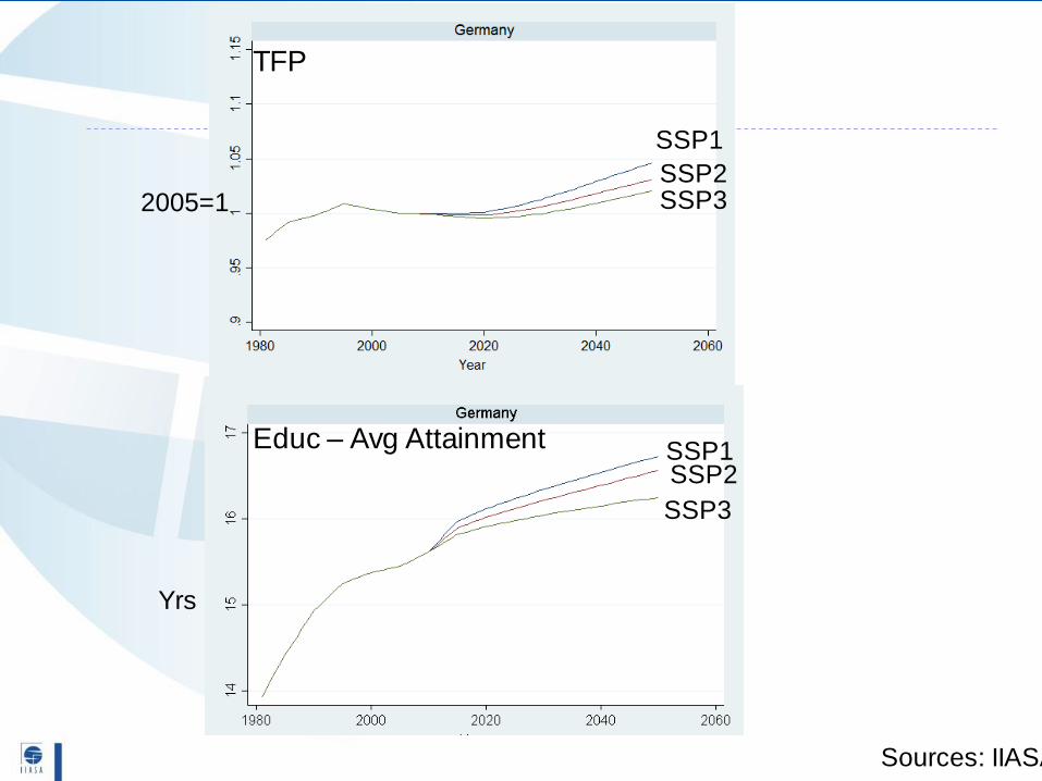
1) Explaining Income Distribution Trends with Petra Sauer, Shonali Pachauri, Jesus Cuaresmo
2) Projecting Income inequality
3) Application to energy/transport demand
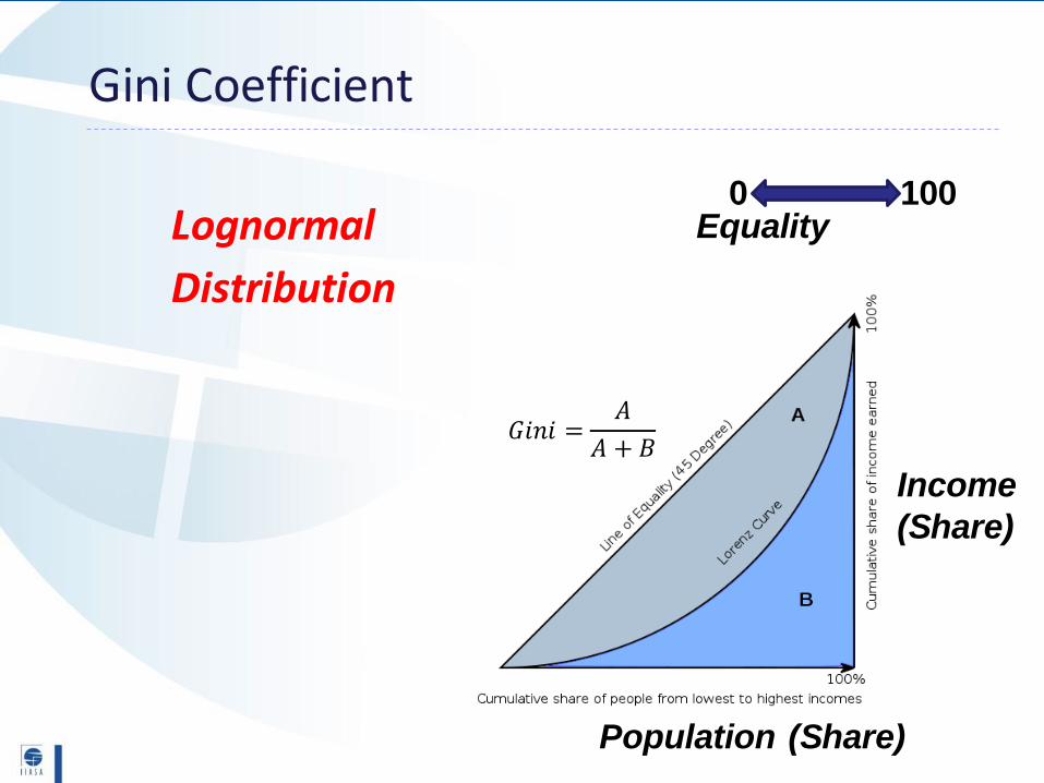
Gini Coefficient
𝐺𝑖𝑛𝑖 =𝐴
𝐴 + 𝐵
0 100EqualityLognormal
Distribution
Population (Share)
Income
(Share)
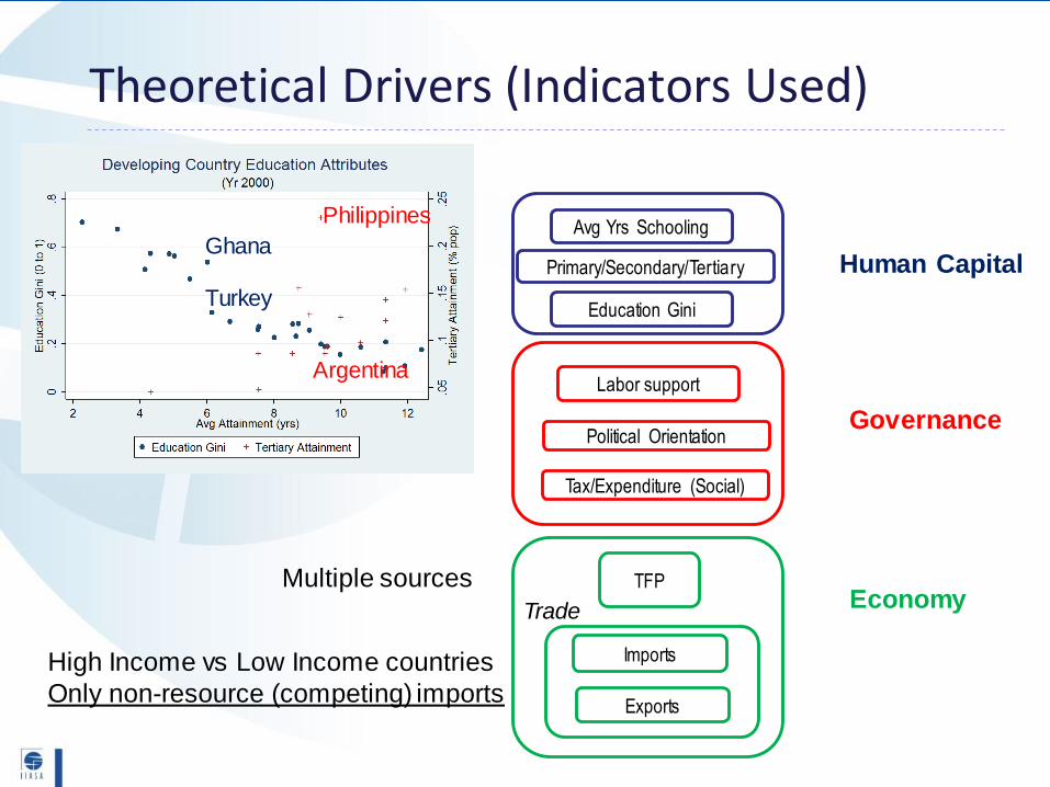
Theoretical Drivers (Indicators Used)
EconomyTFP
Governance
Tax/Expenditure (Social)
Labor support
Political Orientation
Human Capital
Avg Yrs Schooling
Education Gini
Primary/Secondary/Tertiary
Multiple sources
Ghana
Turkey
Philippines
Argentina
Trade
Imports
Exports
High Income vs Low Income countries
Only non-resource (competing) imports
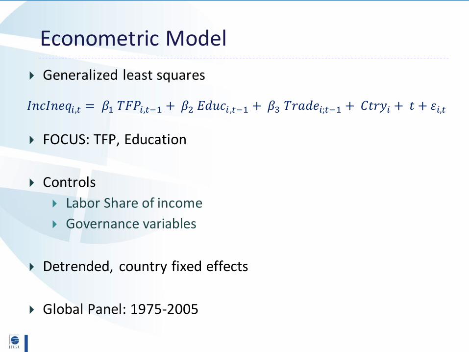
Econometric Model
Generalized least squares
FOCUS: TFP, Education
Controls
Labor Share of income
Governance variables
Detrended, country fixed effects
Global Panel: 1975-2005
𝐼𝑛𝑐𝐼𝑛𝑒𝑞𝑖,𝑡 = 𝛽1 𝑇𝐹𝑃𝑖,𝑡−1 + 𝛽2 𝐸𝑑𝑢𝑐𝑖 ,𝑡−1 + 𝛽3 𝑇𝑟𝑎𝑑𝑒𝑖;𝑡−1 + 𝐶𝑡𝑟𝑦𝑖 + 𝑡 + 𝜀𝑖,𝑡
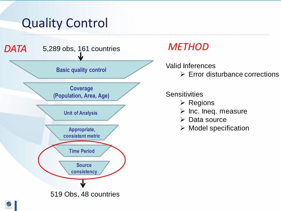
5,289 obs, 161 countries
Basic quality control
Coverage
(Population, Area, Age)
Unit of Analysis
Time Period
Appropriate,
consistent metric
519 Obs, 48 countries
Source
consistency
Quality Control
DATA METHOD
Sensitivities
➢ Regions
➢ Inc. Ineq. measure
➢ Data source
➢ Model specification
Valid Inferences
➢ Error disturbance corrections

Education GiniAdvanced EconomiesOR
Results Summary
34 36.531.5
Gini - Base Case
TFPGlobal
Imports (Low-skilled)Advanced Economies
Scope of Influence Driver (decadal change)+-
Avg Yrs SchoolingGlobal
Global Tertiary Education
Global Primary Education
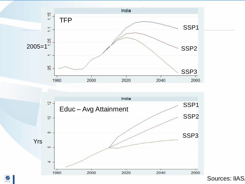
SSP1
SSP2
SSP3
SSP1
SSP2
SSP3
TFP
Educ – Avg Attainment
2005=1
Sources: IIASA
Yrs
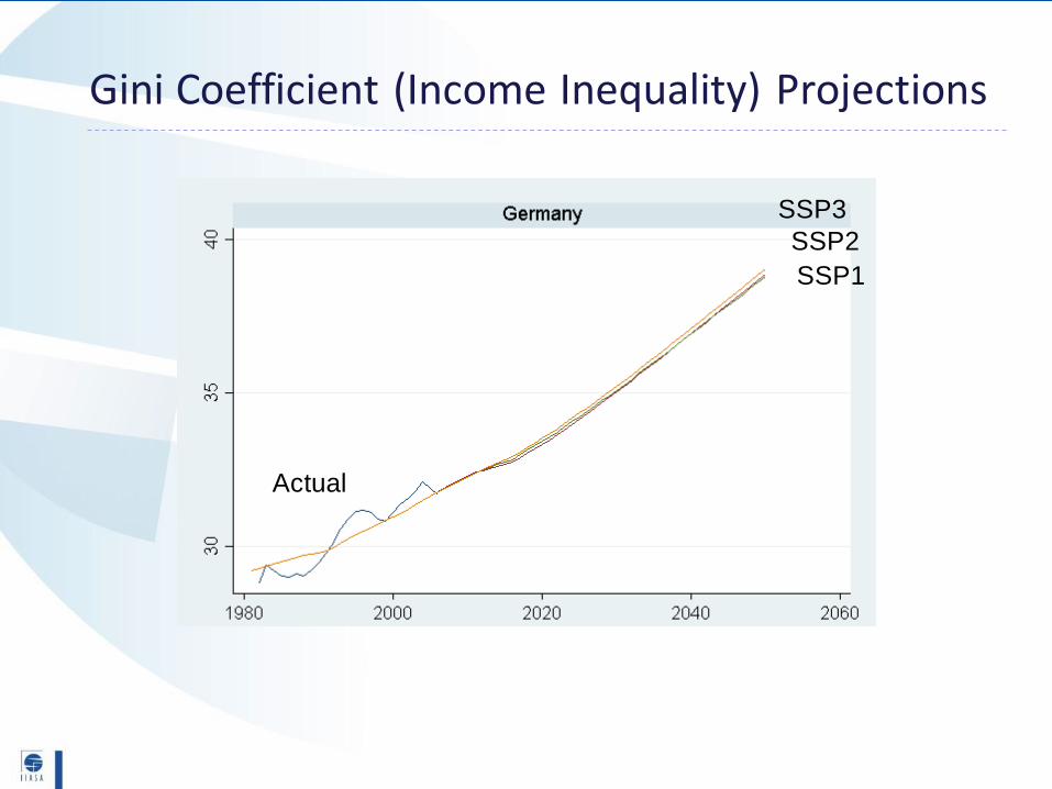
Actual
SSP3
SSP2
SSP1
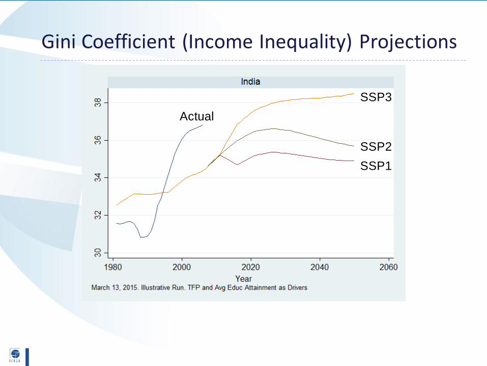
Gini Coefficient (Income Inequality) Projections
SSP1
SSP2SSP3
SSP1SSP2
SSP3
TFP
Educ – Avg Attainment
2005=1
Sources: IIASA
Yrs
Actual
SSP3
SSP2
SSP1
Gini Coefficient (Income Inequality) Projections
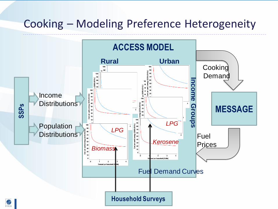
MESSAGE
ACCESS MODEL
Rural Urban
Fuel
Prices
Cooking
DemandInc
om
e G
rou
ps
SS
Ps
Income
Distributions
Population
Distributions
Household Surveys
Fuel Demand Curves
LPG
Kerosene
LPG
Biomass
Cooking – Modeling Preference Heterogeneity
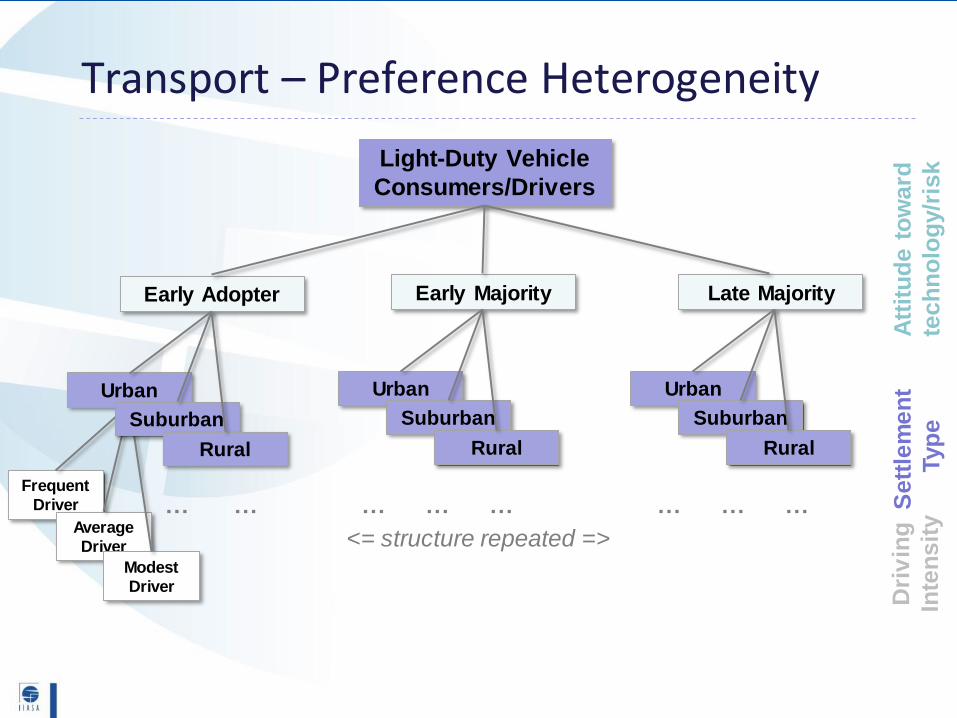
Frequent
Driver
Average
Driver
Modest
Driver
Light-Duty Vehicle
Consumers/Drivers
Early Adopter Early Majority Late Majority
Urban
Suburban
Rural
Urban
Suburban
Rural
Urban
Suburban
Rural
… … … …… … ……
<= structure repeated =>
Att
itu
de
to
wa
rd
tec
hn
olo
gy/r
isk
Se
ttle
me
nt
Typ
e
Dri
vin
g
Inte
ns
ity
Transport – Preference Heterogeneity
Key tasks, milestones
Development of SEH dimensions
Rural/urban pop projections (POP)
Projections of income inequality (ENE)
Model improvements and projections
Projections of fuel use in different SE groups (ENE)
Projections of food demand in SE groups (ESM)
Refined air pollution & GHG emission calculations for different SE
groups (MAG)
Health impact calculations in GAINS (indoor and outdoor exposure to
PM) split up by SE group (MAG)
New indicators of well-being based on SEH parameters
Policy analysis
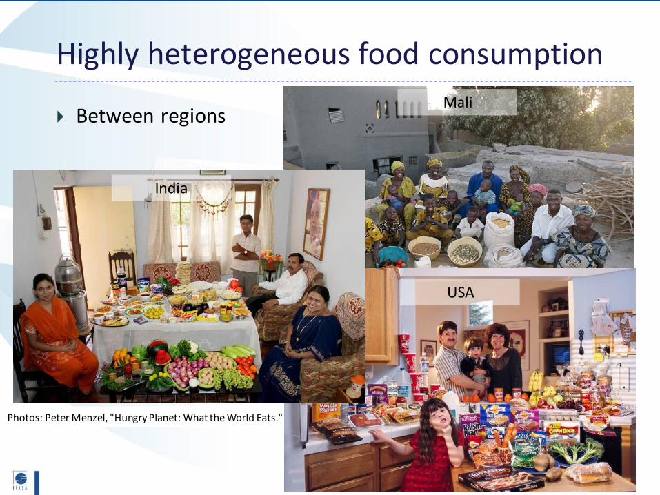
Photos: Peter Menzel, "Hungry Planet: What the World Eats."
Highly heterogeneous food consumption
Between regionsMali
USA
India
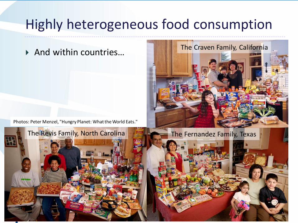
Highly heterogeneous food consumption
And within countries…
Photos: Peter Menzel, "Hungry Planet: What the World Eats."
The Craven Family, California
The Fernandez Family, TexasThe Revis Family, North Carolina
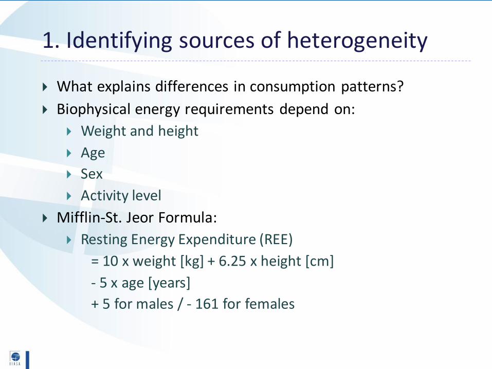
1. Identifying sources of heterogeneity
What explains differences in consumption patterns?
Biophysical energy requirements depend on:
Weight and height
Age
Sex
Activity level
Mifflin-St. Jeor Formula:
Resting Energy Expenditure (REE)
= 10 x weight [kg] + 6.25 x height [cm]
- 5 x age [years]
+ 5 for males / - 161 for females
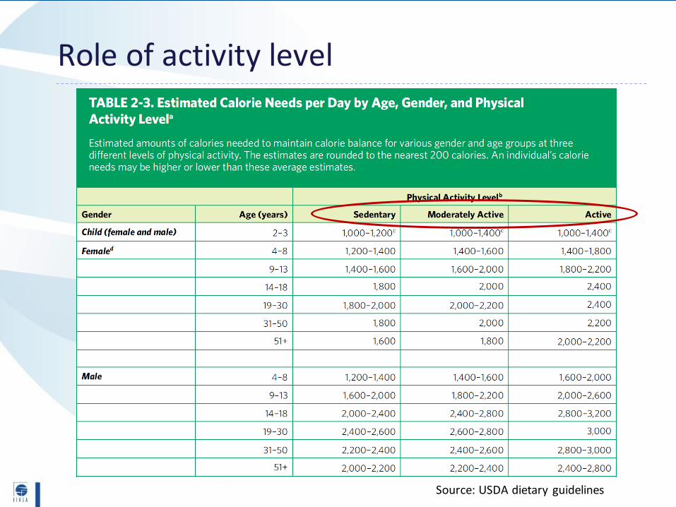
Role of activity level
Source: USDA dietary guidelines
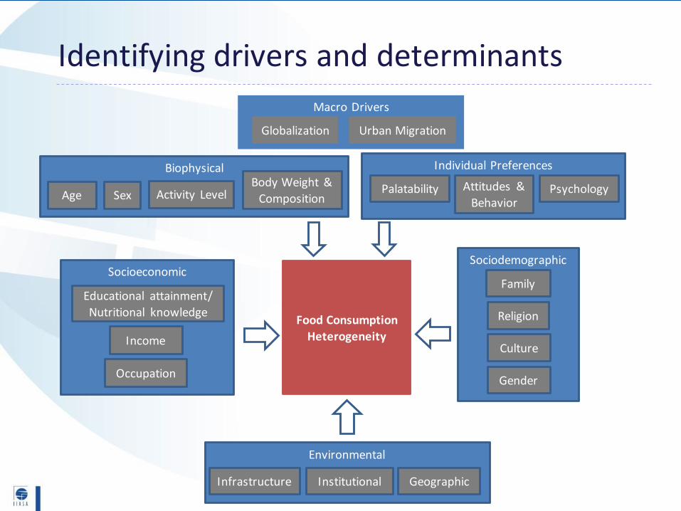
Identifying drivers and determinants
Food Consumption
Heterogeneity
Biophysical
Sex Activity LevelAgeBody Weight &
Composition
Socioeconomic
Educational attainment/
Nutritional knowledge
Income
Occupation
Macro Drivers
Globalization Urban Migration
Sociodemographic
Family
Culture
Gender
Religion
Environmental
Infrastructure Institutional Geographic
Individual Preferences
Palatability PsychologyAttitudes &
Behavior
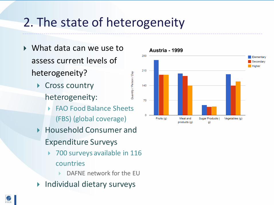
2. The state of heterogeneity
What data can we use to
assess current levels of
heterogeneity?
Cross country
heterogeneity: FAO Food Balance Sheets
(FBS) (global coverage)
Household Consumer and
Expenditure Surveys 700 surveys available in 116
countries DAFNE network for the EU
Individual dietary surveys
3. Projecting food diets using heterogeneity
Current state of heterogeneity will allow more precise
projections through:
Use of SSP drivers already existing for biophysical
determinants : Age
Sex
Inclusion of environmental factors: Income Socioeconomic status
Urbanisation Consumer preferences
Education (already in SSPs)
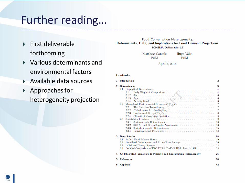
Further reading…
First deliverable
forthcoming
Various determinants and
environmental factors
Available data sources
Approaches for
heterogeneity projection
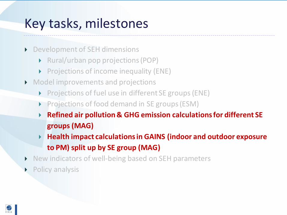
Key tasks, milestones
Development of SEH dimensions
Rural/urban pop projections (POP)
Projections of income inequality (ENE)
Model improvements and projections
Projections of fuel use in different SE groups (ENE)
Projections of food demand in SE groups (ESM)
Refined air pollution & GHG emission calculations for different SE
groups (MAG)
Health impact calculations in GAINS (indoor and outdoor exposure
to PM) split up by SE group (MAG)
New indicators of well-being based on SEH parameters
Policy analysis
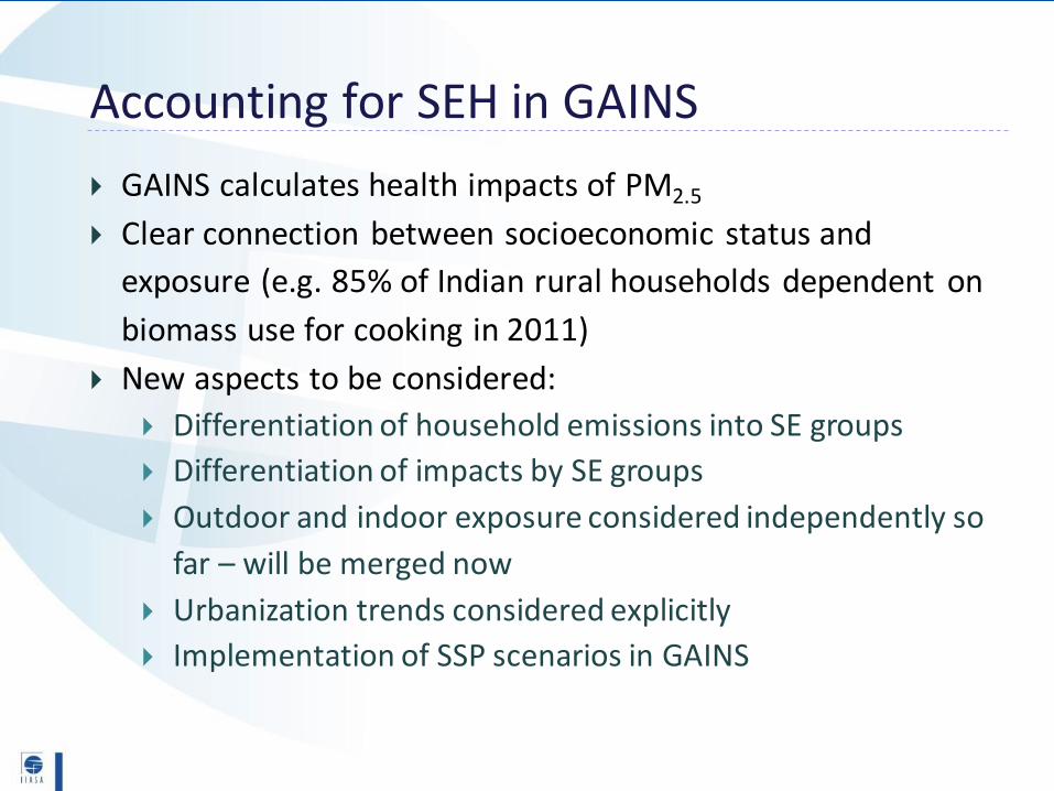
Accounting for SEH in GAINS
GAINS calculates health impacts of PM2.5
Clear connection between socioeconomic status and
exposure (e.g. 85% of Indian rural households dependent on
biomass use for cooking in 2011)
New aspects to be considered:
Differentiation of household emissions into SE groups
Differentiation of impacts by SE groups
Outdoor and indoor exposure considered independently so
far – will be merged now
Urbanization trends considered explicitly
Implementation of SSP scenarios in GAINS
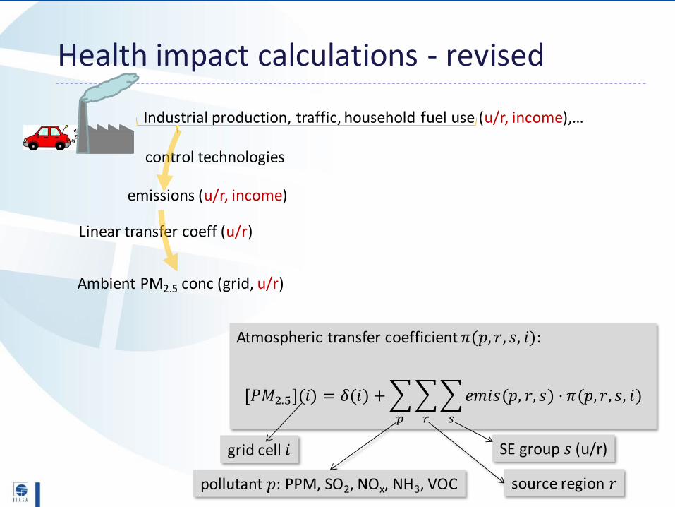
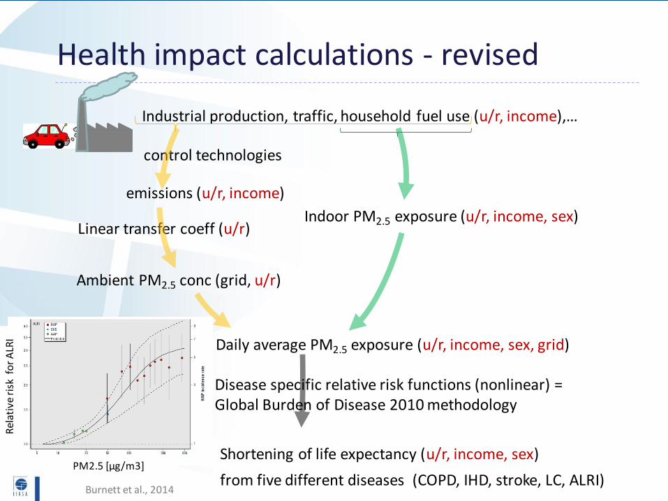
Linear transfer coeff (u/r)
Health impact calculations - revised
emissions (u/r, income)
Ambient PM2.5 conc (grid, u/r)
Industrial production, traffic, household fuel use (u/r, income),…
control technologies
Atmospheric transfer coefficient 𝜋(𝑝, 𝑟, 𝑠, 𝑖):
pollutant 𝑝: PPM, SO2, NOx, NH3, VOC source region 𝑟
grid cell 𝑖 SE group 𝑠 (u/r)
Linear transfer coeff (u/r)
Disease specific relative risk functions (nonlinear) = Global Burden of Disease 2010 methodology
Health impact calculations - revised
emissions (u/r, income)
Indoor PM2.5 exposure (u/r, income, sex)
Ambient PM2.5 conc (grid, u/r)
Daily average PM2.5 exposure (u/r, income, sex, grid)
Industrial production, traffic, household fuel use (u/r, income),…
Shortening of life expectancy (u/r, income, sex)
from five different diseases (COPD, IHD, stroke, LC, ALRI)
control technologies
Burnett et al., 2014
PM2.5 [µg/m3]
Rel
ativ
e ri
sk f
or
ALR
I
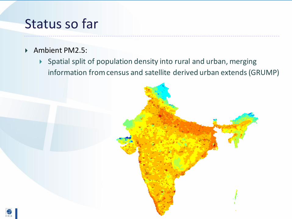
Status so far
Ambient PM2.5:
Spatial split of population density into rural and urban, merging
information from census and satellite derived urban extends (GRUMP)
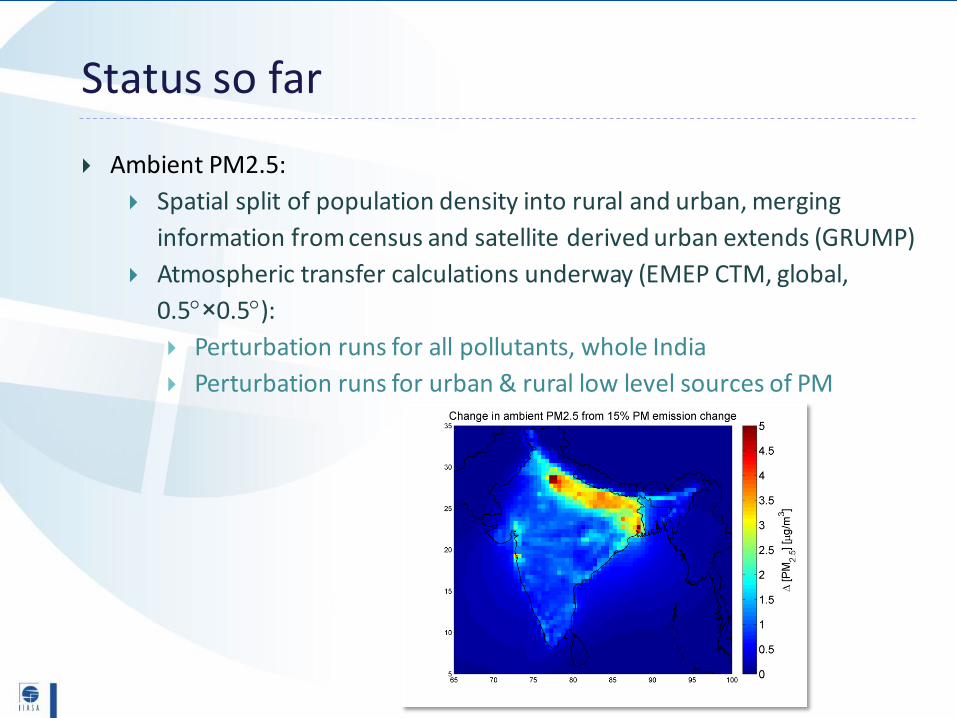
Status so far
Ambient PM2.5:
Spatial split of population density into rural and urban, merging
information from census and satellite derived urban extends (GRUMP)
Atmospheric transfer calculations underway (EMEP CTM, global,
0.5×0.5):
Perturbation runs for all pollutants, whole India
Perturbation runs for urban & rural low level sources of PM
Household PM2.5:
Update of calculation methodology to be consistent with Global
Burden of Disease 2010: calculate mortality via indoor concentrations
& disease specific nonlinear relative risk functions
Conclusion and outlook
First year outcomes:
Primary SEH projections:
Income
Rural-urban
Methodologies to incorporate these dimensions into IIASA
models
Next steps:
Generate secondary drivers (food, energy demand)
New indicators of well-being
Policy analysis

Thank you!
Questions…