soeppapers 472: heterogeneity in the relationship … in the relationship between happiness and age:...

SOEPpaperson Multidisciplinary Panel Data Research

Heterogeneity in the relationship between happiness and age: Evidence from the German Socio-Economic PanelGregori Baetschmann

472 201

2SOEP — The German Socio-Economic Panel Study at DIW Berlin 472-2012

SOEPpapers on Multidisciplinary Panel Data Research at DIW Berlin This series presents research findings based either directly on data from the German Socio-Economic Panel Study (SOEP) or using SOEP data as part of an internationally comparable data set (e.g. CNEF, ECHP, LIS, LWS, CHER/PACO). SOEP is a truly multidisciplinary household panel study covering a wide range of social and behavioral sciences: economics, sociology, psychology, survey methodology, econometrics and applied statistics, educational science, political science, public health, behavioral genetics, demography, geography, and sport science. The decision to publish a submission in SOEPpapers is made by a board of editors chosen by the DIW Berlin to represent the wide range of disciplines covered by SOEP. There is no external referee process and papers are either accepted or rejected without revision. Papers appear in this series as works in progress and may also appear elsewhere. They often represent preliminary studies and are circulated to encourage discussion. Citation of such a paper should account for its provisional character. A revised version may be requested from the author directly. Any opinions expressed in this series are those of the author(s) and not those of DIW Berlin. Research disseminated by DIW Berlin may include views on public policy issues, but the institute itself takes no institutional policy positions. The SOEPpapers are available at http://www.diw.de/soeppapers Editors: Jürgen Schupp (Sociology, Vice Dean DIW Graduate Center) Gert G. Wagner (Social Sciences) Conchita D’Ambrosio (Public Economics) Denis Gerstorf (Psychology, DIW Research Professor) Elke Holst (Gender Studies) Frauke Kreuter (Survey Methodology, DIW Research Professor) Martin Kroh (Political Science and Survey Methodology) Frieder R. Lang (Psychology, DIW Research Professor) Henning Lohmann (Sociology, DIW Research Professor) Jörg-Peter Schräpler (Survey Methodology, DIW Research Professor) Thomas Siedler (Empirical Economics) C. Katharina Spieß (Empirical Economics and Educational Science)

ISSN: 1864-6689 (online)

German Socio-Economic Panel Study (SOEP) DIW Berlin Mohrenstrasse 58 10117 Berlin, Germany Contact: Uta Rahmann | [email protected]

Heterogeneity in the relationship betweenhappiness and age: Evidence from the

German Socio-Economic Panel

Gregori Baetschmann∗

University of Zurich, Department of Economics

This version: May, 2012

Abstract: This paper studies the evolution of life satisfaction over the life course in Germany.

It clarifies the causal interpretation of the econometric model by discussing the choice of con-

trol variables and the underidentification between age, cohort and time effects. The empirical

part analyzes the distribution of life satisfaction over the life course at the aggregated, sub-

group and individual level. To the findings: On average, life satisfaction is mildly decreasing

up to age fifty-five followed by a hump shape with a maximum at seventy. The analysis at

the lower levels suggests that people differ in their life satisfaction trends, whereas the hump

shape after age fifty-five is robust. No important differences between men and women are

found. In contrast, education groups differ in their trends: highly educated people become

happier over the life cycle, where life satisfaction decreases for less educated people.

Keywords: aging, life satisfaction, well-being, happiness methodology

JEL Codes: C23, I31, D91

∗ I would like to thank Rainer Winkelmann for many helpful suggestions which improved this article.Address for correspondence: University of Zurich, Department of Economics, Zurichbergstr. 14, CH-8032Zurich, Switzerland, T+41 44 634 2295, k [email protected]

1 Introduction

This paper contributes to the recent literature on the evolution of individual satisfaction

over the life cycle.1 The most prominent hypothesis is that of a U-shape relation between

age and happiness. Detailed studies of the relationship, especially for Germany, have

confirmed the U-shape over a long range of the life course, but have found another downturn

at the end of life (Wunder et al. (2009), Van Landeghem (2009), Fischer (2009), Gwozdz

and Sousa-Poza (2009)). Knowing how life satisfaction evolves helps to answer questions

like “what is the probability that well-being decreases in the next ten years for a currently

40 year old woman?” or “how happy will I be in twenty years?”. Further, it can help to

optimize saving decisions. For instance, taking into account the U-shape could help people

avoid oversaving for old age.

A key shortcoming of the previous literature is the neglect of heterogeneity in the

relationship between age and life satisfaction. With few exceptions (Mroczek and Spiro

(2005), Schilling (2006)), the conducted studies have only looked at the central tendency of

well-being over the life course at the aggregate level. But seeing a U-shape for the average

does not mean that such a relationship is representative for the individual. It is possible

that a U-shape results from averaging over individual life cycle paths, which are themselves

not U-shaped. Moreover, it is possible that age influences the whole distribution of life

satisfaction and not only the location.

Using the longest running panel household survey with continuous information on life

satisfaction so far, the German Socio-Economic Panel (SOEP), it becomes possible to

trace individual satisfaction levels for up to 26 years, and hence, in principle, to estimate

the relationship between age and life satisfaction at the individual level using time series

methods. A further advantage of the SOEP data is that they include information on the

entire adult population (those age 20 or above), including the very old. For example seven

per cent of the sample (more than 20’000 observations) are older than 70 years. This broad

coverage is important for testing the hypothesis of a second turning point, i.e. a decrease

in life satisfaction at high age.

1The terms life satisfaction, happiness and well-being are used interchangeable in this paper. For a

summary of the literature, see for example Blanchflower and Oswald (2007).

1

The key contributions of the paper are as follows: First, I replicate the findings in the

literature regarding the relationship between age and average life satisfaction in a general

semi-parametric model. Second, I provide an extended analysis of heterogeneity in the life

course of satisfaction using evidence from four types of models: dispersion as dependent

variable; analysis by subgroups; latent class analysis; and individual level regressions.

The findings of the paper are compatible with a U-shape over most of a person’s adult

life time. However, a more detailed analysis reveals a mild downward trend up to around

55, followed by a distinct increase. After the age of 70, the curve is clearly falling. The

study of the distribution of well-being shows a mixed picture. The fraction of people with

a very high satisfaction level is falling over the life course. To a lesser extent, this is also

true for the fraction of people with a low satisfaction level. Combined, this results in a

decreasing dispersion in life satisfaction between people over the life course.

Whereas men and women show a very similar development over the life course, education

groups differ strongly. People with low education seem to suffer from a steady decline in life

satisfaction, while well educated people become happier. However, the hump shape after 55

can be found in all education groups. The result of the finite mixture model confirms the

hypothesis that heterogeneity between people can be primarily found in the trend over the

life cycle, whereas less heterogeneity exists in the hump shape after 55. Another important

finding is that the length a person spent in the panel strongly affects the response. This

duration effect, the high variance at the individual level, and the rough measurement of life

satisfaction are probably the reasons why investigating the relationship between age and

life satisfaction at the individual level provides no clear insights.

2 Modeling life satisfaction over time

Any study attempting to identify and estimate the relationship between age and life sat-

isfaction needs to take a stance on a number of issues. First, what variables to condition

on; second, how to deal with the fundamental identification problem between the effects

of age, cohort and time, and whether or not to include individual fixed effects; third, to

define the relevant level of aggregation; and fourth, what assumptions to make regarding

the econometric model, for a given set of regressors: parametric versus semi-parametric,

2

and linear regression versus non-linear ordered probit or ordered logit models. The follow-

ing sub-sections provide a discussion of each of these four points, their treatment in the

existing literature as well as the position adopted in the present paper.

2.1 Conditional vs. unconditional effects

This paper focuses on the question of how life satisfaction has evolved over the life course

in Germany in recent years, because I think that results from such an inquiry can be

extrapolated and help predicting the evolution of life satisfaction in the near future in

Germany and other advanced industrial countries. To get an answer to the question of

how life satisfaction has evolved, one essentially needs to follow different people and record

their well-being levels. This is the unconditional approach.

In the conditional approach, the researcher is trying to hold some individual level char-

acteristics – like income, health or marital status – constant in order to get a “ceteris

paribus” interpretation. But these variables are potential channels through which age af-

fects life satisfaction. Holding individual level variables constant can therefore be highly

misleading. Comparing a 50 year old man with three children and a monthly income of

$20,000 with a man with the same characteristics but only age 20, hardly helps to identify

the effect of age on life satisfaction. The focus on the unconditional age effect is in line

with the view expressed by Glenn (2009), Easterlin (2006), and Easterlin and Sawangfa

(2007), and in contrast to the approach of Blanchflower and Oswald (2008). Of course,

if it is the goal of the analysis to identify the channels through which age influences life

satisfaction, it is meaningful to include individual level covariates. This paper concentrates

on the evolution of well-being over the life course per-se, and not on the causal channels.

Nevertheless, there are some variables for which one should control in the econometric

model. Year of birth is correlated with age and has probably also an effect on life sat-

isfaction, but is surely not a channel through which age influences happiness. Thus the

econometric model should control for cohort effects (see e.g. Blanchflower and Oswald

(2008) for a discussion). There is also recent evidence that “panel learning” can have a

substantial effect on the response behavior by persons. Panel learning means that people

change their responses over time just because they have participated repeatedly in the sur-

3

vey, i.e., even if the underlying feature one wants to measure is unchanged. In the context

of life satisfaction, Kassenboehmer and Haisken-DeNew (2010) found a negative effect of

time spent in the panel. They conjecture that confidence in the interviewer may rise with

each additional interview, which leads to more honest (in this case lower) answers to the life

satisfaction question. Interestingly, this panel duration effect has been ignored by much of

the previous literature, including the studies by Wunder et al. (2009) and Ree and Alessie

(2011), putting a serious question mark behind the findings of these papers.

A further controversial question is whether or not one should control for time effects.

The time effect is often split into a shock (for example business cycle) and a trend (e.g.

long run economic growth). For example, if the observation period falls together with an

economic recession, it looks as if people become unhappier as they get older. However, if

the observation period is long enough and different cohorts are tracked, there is no reason

why the shocks should be correlated with age. Regarding the long-term trend, it seems

pointless to compute age-profiles that exclude the long-term trend, as time and age move

in unisono. Arguably, therefore, one should not condition on the trend, but rather focus

on the combined effect of age and time in order to predict future age-profiles.

2.2 A fundamental identification problem

In an additive model with age, cohort and time, it is not possible to disentangle the linear

effect of these three variables, whereas the deviation from the linear effects of each of the

three variables is identified. This was formally shown in McKenzie (2006) in a general

non-parametric framework. The essence of the argument can be demonstrated in a simple

model with linear and quadratic terms:

y = β0 + βaage+ γaage2 + βccohort+ γccohort

2 + βttime+ γttime2 + ε (1)

Because age = cohort+time, there exists a multicollinearity problem between the three

variables. This means that it is not possible to identify βa, βc, and βt separately. If one

of the three linear terms is dropped, the regression can be run, but the coefficient on the

other two remaining linear terms combine their own effect and the effect of the dropped

variable. Clearly, age2 6= cohort2 + time2 (unless one of the terms on the right is zero),

and hence there is no problem of multicollinearity here. The same holds true for higher

4

order terms. Thus the linear effect of the three variables cannot be disentangled, whereas

deviations from the linear effects are identified.

Ree and Alessie (2011) argue that it is thus not possible to assess the hypothesis of

a U-shape but only the hypothesis of a convex relationship between age and happiness.

Convexity is a weaker claim than U-shape. In the simple example above where happiness

is a linear function of age and age2, convexity means that γa > 0. A U-shape relationship

further requires that a minimum exists (βa < 0), and that the minimum lies in the observed

age range, thus −βa/(2γa) ∈ [20, 80]. Convexity is necessary but not sufficient for a U-

shape. If βa is not identified, it is hence only possible to test one requirement of a U-shape,

namely the convexity, but not to test for a U-shape itself. Of course, if convexity is rejected,

then so is the U-shape.

The argument of Ree and Alessie (2011) is formally correct. However, one has to ask,

if this unidentified isolated age effect is really the effect we are interested in. As argued

above, this age effect, which is fully disentangled from the time effect, is not interesting

and has no clear interpretation. The underlying reason for the lack of a meaningful or

causal interpretation is that it is not possible to become older without proceeding in time.

In contrast, the age effect combined with the estimated linear time effect is interesting and

useful. For example, if a person wants to predict his well-being level in ten years, he is not

interested in the isolated effect of age but in the total effect of age and time. For him, it

is not meaningful to assume that the social and economic conditions, for which the time

variable is a proxy for, will be the same as today. And the best estimate for the effect of

these changing conditions in the future is probably the linear time effect in the last years.

This effect is estimated by dropping time from (1), in which case age estimates βa + βc.

Another question is if one should include individual fixed effects into the econometric

model. It can be argued that this does more harm than good in the present case. First, there

is no obvious reason (for example a selection problem), why one should include individual

fixed effects into the econometric model. If the sampling process and the cohorts are stable

over time, the cohort variable will control for systematic correlations between age and the

individual fixed effects. Second, including individual fixed effects into the econometric

model leads to a high conditional correlation between age and panel duration. The panel

duration effect would then be identified only from people who do not take part in the survey

5

in one year but return in the next. There are relatively few such cases. Without individual

fixed effects, the main variation in the panel duration results from various refreshment

samples, where new subjects of various ages were recruited at different points in time.

2.3 Aggregation problem

Phenomena at the aggregate level or mean effects are often crucial for policy recommen-

dations. However, for explaining and understanding a phenomenon in the aggregate, it is

important to link them to patterns on the individual level. In the context of the relation

between age and happiness, the difficulty is that different mixtures of distinct individual

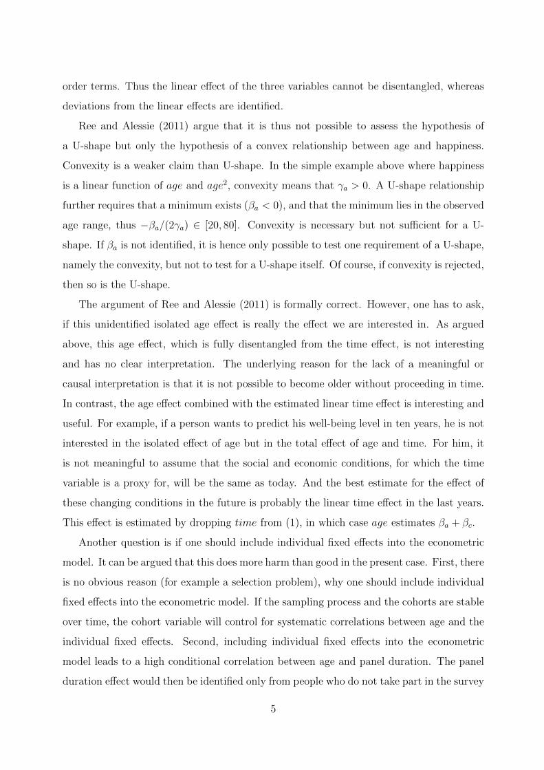
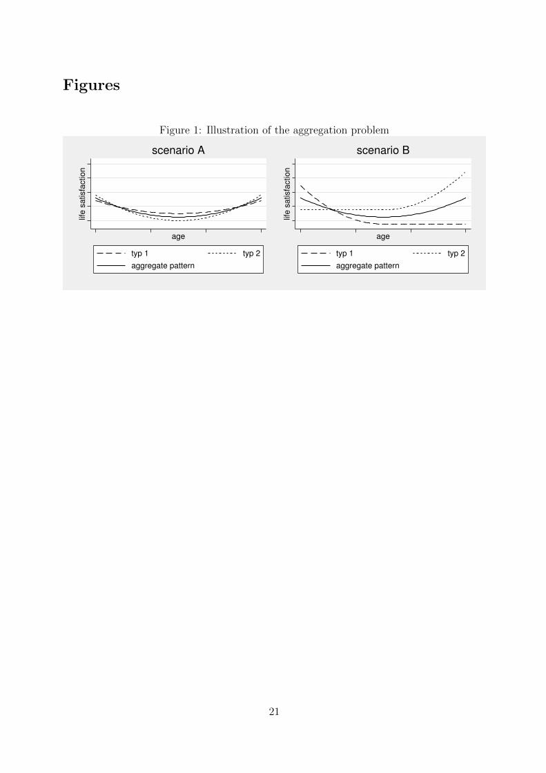
life course paths can lead to the same aggregate pattern. This problem is illustrated in

Figure 1. In scenario A, the population consists of two types, both with a share of 50%.

For both types, the evolution of life satisfaction is U-shaped, but they differ in the level

and curvature. In scenario B, the population consists again of two different types with

equal shares. In contrast to the first one, none of the two types has a U-shaped pattern.

However, the relation between age and life satisfaction in the aggregate, as represented by

the solid line, is the same in both scenarios.

−−−−−− Figure 1 about here −−−−−−−

It is simply not possible to say something about patterns at the individual level by only

looking at the aggregate picture. Thus “midlife crisis”, for example, would only be a valid

explanation for the U-shape in the aggregate in scenario A. An explanation for the second

scenario would be that people differ in their discount rates and can choose between two

different life cycle paths. People with a high discount rate choose the path with the higher

initial life satisfaction level, while people with a low discount rate choose the path with the

higher average score.2

The literature so far has focused on the aggregate pattern. To the best of my knowledge,

the only studies in the age-happiness literature which give some attention to this problem

are Mroczek and Spiro (2005) and Schilling (2006). Another study in the happiness lit-

2This argument assumes that satisfaction is period specific, i.e., anticipation of future increases or

reductions in satisfaction do not enter present satisfaction.

6

erature touching this problem is the paper of Clark et al. (2005), which tries to capture

heterogeneity in the income effect on life satisfaction with a finite mixture model.

2.4 Econometric model and estimation

To investigate the relation between age and life satisfaction, an additive model is used

throughout the paper. In this section, I describe the basic version of the model that focuses

on aggregate patterns, as represented by the conditional expectation. In later sections, the

model will be modified appropriately in order to enable the study of heterogeneity.

As discussed previously, the included regressors are age (a), year of birth (c for cohort),

year of the interview (t for time) and the time spent in the panel up to the interview (d for

duration). The dependent variable is a measure of life satisfaction and is denoted by y. A

flexible additive model for the expectation of y can be written as:

E(y|a, c, t, d) = β0 +80∑

k=20

βakIak +

1989∑k=1904

βckIck +

2009∑k=1984

βtkItk +

26∑k=1

βdkIdk , (2)

where β0 denotes the constant and I the indicator function (thus Iak , for example, equals

1 if the age variable is equal to value of the indicator k). The model includes a dummy

for each category of the four variables, and β stands for the effect of the corresponding

dummy.

Two sorts of restrictions have to be imposed to enable estimation:

max(x)∑k=min(x)

βxk = 0 for all x ∈ {a, c, t, d} (3)

2009∑k=1984

βtkk = 0. (4)

Equation (3) restricts the total effect of each variable to zero and hence avoids multi-

collinearity between the dummies. It is functionally equivalent to dropping one dummy of

each variable. The second restriction – equation (4) – ensures that the linear effect of the

time variable is equal to zero and thus avoids multicollinearity between the linear effects of

age, cohort, and time (cf. section 2.2).

The identified linear effects can be directly estimated by reformulating the econometric

model. Including a separate term for the trend of each variable and using the identity

7

time = age+ cohort results into the following model:

E(y|a, c, t, d) =β0 + (βa + βt)a+80∑

k=20

βakIak + (βc + βt)c+

1989∑k=1904

βckIck+

2009∑k=1984

βtkItk + βdd+

26∑k=1

βdkIdk , (2’)

where β’s without subscript denote the trends. To enable estimation, restriction (3) and

restrictions equivalent to (4) on cohort, age and duration in addition to time are imposed.

Because the variable time was replaced by age plus cohort, the variables age and cohort

estimate their own linear effect plus the time trend.

Both formulas represent the same model, which can be estimated by ordinary least

squares (OLS). The well-being variable is usually described as ordered, and the median

is normally viewed as the right statistic to characterize the location of an ordered vari-

able.3 The mean, however, has the advantage to be more sensitive to small changes in the

distribution. Previous studies – Ree and Alessie (2011), Wunder et al. (2009), and Van

Landeghem (2009) – have found a magnitude of less than one point on the eleven point

scale in Germany. Thus it is possible that the location of the distribution changes system-

atically over the life course, whereas the median is constant. For this reason, the mean is

used to study the evolution of average life satisfaction. To allow for dependence between

repeated observations of one individual, cluster corrected standard errors are reported.

3 Results

3.1 Data description

The paper uses data from the German Socio Economic Panel (SOEP). The unique feature

of this data set is its long time dimension. At present, it is possible to follow some people

for 26 years, from 1984 to 2009. The analysis is conducted with unweighted observations

of people, who live in (former) West-Germany and are between 20 and 80 years old. Life

3Of course, one could also estimate conditional probability models such as the ordered logit or ordered

probit model. The case for such models is not very persuasive in the present context, where there are eleven

numbered outcomes (from zero to ten) and cardinal interpretations are desired. See Ferrer-i-Carbonell and

Frijters (2004) for a comparison of OLS versus ordered response models in this context.

8

satisfaction is ascertained with the question “How satisfied are you with your life, all things

considered?” that is always asked at the end of the interview.4 The response is measured on

an eleven point scale ranging from 0 (completely dissatisfied) to 10 (completely satisfied).

Table 1 shows the distribution of the life satisfaction score and summary statistics of the

employed variables. The average happiness score lies slightly over 7, where about 50%

of the answers are concentrated on the categories 7 and 8. In contrast, only 8% have a

life satisfaction score below 5 (the midpoint of the scale). By construction, people in the

sample are born between 1904 and 1989. Nearly half of them are women.

−−−−−− Table 1 about here −−−−−−−

3.2 Mean

Based on equation (2) and the two technical restrictions (3) and (4), the development of

average well-being over the life cycle is analyzed. Figure 2 presents the regression results.

As discussed in section 2.2, it is not possible to estimate the linear effect of age, cohort and

time separately, whereas the linear effect of duration in the panel poses no problem. As

argued above, this underidentification is not as severe as other papers suggest, but it is not

clear how to report the results. Because this paper focuses on the age effect, the time trend

coefficient is restricted to zero (equation (4)) and is thus captured in the age and cohort

effect curves. The terms “age effect with trend”, “cohort effect with trend”, respectively

“time shock effect” are used to refer to the mapped impacts. Additionally, the estimation

results for the isolated linear effects (equation (2’)) are stated in Table 2. The estimated

trends are, in contrast to Ree and Alessie (2011), very small. The linear effects of age and

time (βa + βt), and cohort plus time (βc + βt), respectively, are both 0.003 per additional

year. The reason for the differences between the results of Ree and Alessie (2011) and this

study is the inclusion of duration in the panel as an additional control variable. Because

the magnitude of the linear effects is so small, the changes in the graphs would only be

4In German: “Wie zufrieden sind Sie gegenwartig, alles in allem, mit Ihrem Leben?”

9

minor if the drifts would be excluded.

−−−−−− Table 2 about here −−−−−−−

The age effect with trend can be characterized as U-shaped. However, such a description

is somewhat oversimplified. A closer inspection shows that the picture fits nicely to previous

research results. There is a small but steady decline in the happiness score between age 20

and 55. After this trough – which coincides with the minimum in a sample of eight European

countries found by Blanchflower and Oswald (2009) – average happiness increases strongly

until the age of 70. Thereafter, the average score falls sharply. Wunder et al. (2009) and

Van Landeghem (2009) have also found a local maximum at age 70. The total magnitude

of the effect (0.4) is small and thus in line with, for example, Kassenboehmer and Haisken-

DeNew’s (2010) doubt about the U-shaped relationship. The effect without linear trend is

very similar to the one reported by Ree and Alessie (2011) who also used the SOEP, albeit

for the shorter 1986-2007 period. The reason for the fall at the end of life is likely decreasing

health. Explaining the increase after 55 is more difficult and calls for more research.


The cohort profile with trend, displayed in the lower left panel of Figure 2, is slightly

increasing. But otherwise no clear or interesting pattern emerges. This is perhaps also due

to the low precision of the estimates which renders the interpretation difficult. The time

shock profile mirrors the business cycle. There is a distinct peak right after the German

reunification. The low in the first decade of the new millennium overlaps with the burst

of the ICT bubble. The correlation between the estimated shocks and the GDP growth in

the previous year is over 60%.5 Again, a very similar profile was found by Ree and Alessie

(2011). Among all included variables, the time spent in the panel (duration) has clearly

the highest impact on reported happiness. The picture suggests a negative linear effect,

corroborating the earlier findings of Kassenboehmer and Haisken-DeNew (2010).

5Based on calculations using World Bank (2011) data.

10

3.3 Distribution and dispersion

To analyze the distribution of the happiness variable, the baseline model – equation (2)

together with restrictions (3) and (4) – is applied separately to each category of the life-

satisfaction variable. These linear probability models estimate the effect of age on the

probability of having a given life satisfaction score, for example “nine”, accounting for year

of birth, time shocks, and duration. Figure 3 shows the results for the age effect with

trend plus constant, where some categories are combined for simplicity. The results for

the controls are not shown. There seem to be no common pattern behind the six curves.

The probability of being totally happy (having a value of 10) is steadily decreasing over

the life course with a plateau between 60 and 65. This decrease can be made responsible

for the downward slope of average life satisfaction between 20 and 55 as well as the fall

after 70. The decreasing probability of the highest category implies an offsetting increase

for the other categories. The greatest change occurs in the probability of having an 8. The

hump shape in the mean curve starting at 55 can largely be ascribed to the temporary

decline in the probability of having a 3, 4 or 5, i.e. being rather “dissatisfied”. Compared

to the rather small absolute changes in average happiness, the changes in the distribution

are large. The predicted probability of reporting a 10, for example, decreases by fifteen

percentage points over the life cycle.


These findings of decreasing probabilities of low and high life satisfaction scores over

the life course imply a steadily shrinking dispersion. To illustrate this, the baseline model

is applied to the absolute deviation of the residuals from the mean life satisfaction score

regression. Figure 4 shows the results. Dispersion is steadily decreasing in age and is

smaller for younger cohorts. As discussed, the linear trend of age, cohort and time cannot

be disentangled. The most probable explanation for the two decreasing tendencies is a

time trend toward more equality, which is mirrored in the graph for the age and the cohort

effect. These findings are in line with those of Stevenson and Wolfers (2008) who reported

that the dispersion in happiness was shrinking between 1972 and 2006 in the USA, and that

happiness is less equally distributed within older cohorts. Compared to age and cohort,

11

duration in the panel and time shocks have only a small effect on dispersion.


3.4 Relation in different subgroups

To study heterogeneity in the relationship between age and life satisfaction, the baseline

model – equation (2) under restrictions (3) and (4) – is applied to different subgroups. I

consider groupings based on gender and years of education. Among the two, gender is

clearly exogenous, whereas education may be affected by self-selection.


Figure 5 shows the regression results for men and women. The resemblance of all four

curves is quite striking. For both genders, the age curve has a minimum at around 55,

followed by a distinct hump shape. The greatest difference in the age effect between the

sexes can be observed until 55. Where the curve is clearly decreasing for men, the profile

is flatter and perhaps upward sloping between 20 and 30 for women. Further, the positive

trend in the cohort effects is stronger for women. Otherwise, there are no noticeable

differences between the curves.


To study heterogeneity depending on education, the population is split along the edu-

cation dimension into six groups of roughly equal size. Figure 6 shows the results of the

age effect with trend in the baseline model for all types. Two patterns stand out: First,

the hump at the end of life can be found in all six groups. Second, the linear trend changes

systematically. Life satisfaction for the least educated people is clearly downward sloping.

However, the negative trend gets less pronounced as education increases, and the drift for

people in the most educated group is even positive. Estimating the baseline model for the

mean and including an age-education interaction term confirms the finding that the trend

for better educated people is more positive (results not shown in the paper). However, one

12

has to be cautious in interpreting the results. Because people can choose education at the

beginning of life, one cannot infer that education causes these different life cycle paths. It

is also possible that personality traits, like self-discipline, lead to different life course paths

as well as variation in education outcomes.

3.5 Finite mixture model

Finite mixture models allow to model heterogeneity depending on unobservable class mem-

bership, which does not necessarily depend on observable characteristics like gender or

education (a standard reference for finite mixture models is McLachlan and Peel (2000);

for previous happiness applications see Clark et al. (2005) or Bruhin and Winkelmann

(2009)). Estimating such a model requires specifying the conditional distribution and not

just the mean. Because the specification of the distribution is somewhat arbitrary, two

different models are estimated, a linear model with normally distributed error terms and

an ordered logit model. Where the first model is a direct extension of the linear model

employed earlier, the second has the advantage of respecting the support of the dependent

variable (0, 1, . . . , 10). If a simplified version of the model is estimated, both procedures

lead to the same qualitative conclusions. Thus I present only the results of the normal linear

model. The log-likelihood contribution of person i, who is represented with Ti observations,

in the simplified model is

log

[G∑g=1

(πg

Ti∏t=1

1

σgφ

(yt − βg0 −

∑80k=21 β

a,gk Iatk −

∑26k=2 β

d,gk Idtk

σg

))], (5)

where φ(.) denotes the density function of a standard normally distributed random variable,

σ the standard deviation and πg the probability of belonging to class g. There existG groups

and the subscript g of the parameters indicates that they depend on group membership.

Otherwise, the same notation as in equation (2) applies.6 The log-likelihood function is

6The estimated model imposes the restrictions that the time and cohort variables have no effect. This

facilitates convergence and is compatible with the theoretical independence between the time shocks and

age, and the empirical finding that the cohort effect has no systematic effect on mean life satisfaction

(section 3.2). Further, people age 20 polled the first time (hence duration=1) are defined as the base

category.

13

maximized with the EM-algorithm.7

Figure 7 shows the estimated effect of age on life satisfaction for one to four latent

classes. The upper left graph shows the results for the model with only one class. It is

evident that the interpretation of a U-shape followed by a hump shape does not change if

the time shocks and the cohort variable are excluded. The striking result of the remaining

graphs is that the hump shape after 55 can be found in all latent groups, regardless of

the number of allowed classes. The trends over the life cycle, however, differ between the

groups. The largest group is always the one with no clear drift.


3.6 Individual patterns

The study of the relation between age and life satisfaction on the individual level is com-

plicated by three factors. First, the maximum length one can follow a person is 26 years

and it is therefore not possible to study satisfaction over the whole life cycle for any one

individual. Second, the variance of the error term is large relative to the expected changes

of the mean happiness score. At the individual level, the smallest possible change of the

dependent variable is one point. This exceeds the maximal average effect found over the

life cycle. Third, duration in the panel has a large effect. But on the individual level, it is

not possible to disentangle the duration from the age effect in a credible manner.

The empirical inquiry at the individual level starts therefore by studying the fraction

of people at a certain age, who report at that age a larger (or smaller) happiness than at

any other time over the previous ten years. This restricts the analysis to individuals who

are observed for at least eleven years. The share of people in the population experiencing

a minimum (maximum) is probably overestimated (underestimated), because this analysis

ignores the duration effect. However, it is still possible to determine whether the finding

of a U-shape followed by a hump shape prevails at the individual level. Figure 8 shows

the results. First a short explanation how to read the graph: A value of 20% at the age of

7The R-program FlexMix by Bettina Gruen and Freidrich Leisch (2008) was used to estimate the linear

finite mixture model.

14

thirty means that one out of five people, who are at least observed between age twenty to

thirty, experiences a minimum at thirty in this period (the minimum has not to be unique).

The confidence intervals are not shown for ease of readability (but each estimate is based

on more than 1000 observations). The fraction of minimums almost always exceeds the

fraction of maximums. The obvious explanation is the neglected duration effect. There

is no clear trough at 55 but the fraction of minimums decreases and the proportion of

maximums goes up after this age. These small changes are more than offset by the trends

after age 68. The fraction of minimums is nearly exploding, and the fraction of maximums

shrinks.


Because the U-shape hypothesis and the corresponding trough have received much at-

tention in the literature, the distribution of minimums for people who are observed between

age 48 and 62 are shown in Figure 9, these are about 1000 individuals. The distribution is

nearly uniform, with a slight increase with age. This slight trend can again be explained

by the neglected negative duration effect. The general pattern suggests that only a small

fraction of the individuals reach the minimum at exactly 55.


To further study heterogeneity at the individual level, a separate model is estimated for

each individual and each possible interval of length eleven (thus, in general, more than one

model per individual). To keep it simple, the model consists of two linear age terms, one for

the first and one for the second half of the interval. Each regression is then characterized as

hump shaped (if the first linear term is positive and the second one is negative), U-shaped

(if the first linear term is negative and the second one is positive), increasing or decreasing

(depending on if both terms are positive or negative). If well-being does not systematically

change over the life course, the four curves should be flat. But this is obviously not the

case, as can be seen in Figure 10. The picture largely confirms the finding that the hump

shape after 55 is the dominant pattern. The fractions are nearly stable until 50 where the

U-shape and the increasing patterns start to gain shares. At 55, the fraction of U-shape

15

types reaches a maximum and the fraction of hump shape types a minimum. Shortly after

60, the fraction of decreasing types becomes more and more important.


4 Conclusion

This paper studies the relationship between age and self-reported well-being not just at

the average level, as customary in prior research, but also at the individual level, analysing

the differences between individual life cycle paths. The inquiry of heterogeneity at the

individual level, while of substantial interest, is hampered by the rough measure of life

satisfaction and the related high volatility in individual life cycle paths, as well as by the

strong duration effect. Nevertheless, it is safe to conclude that a life cycle pattern with two

turning points is prominent at the individual level as well.

Insights into the average evolution of life satisfaction and group differences between

individual life cycle paths are more robust. Mean life satisfaction is steadily declining

between 20 and 55. After this low, happiness increases strongly until the age of 70, where it

starts to fall sharply. The driving force behind the hump shape after 55 is the temporarily

diminishing share of rather unsatisfied people. The mild downward trend, on the other

side, is mostly due to the falling probability of the “completely satisfied” category. The

dispersion in well-being is decreasing in age and year of birth. An explanation of this

pattern is the time trend toward more equality.

While the happiness trend over the life course differs between groups of people, whereas

the form of the relationship (thus the deviation from the linear trend), is rather stable,

namely a hump shape after 55 with a peak at around 70. This conclusion is based on the

regression for different education groups as well as the results of the finite mixture model.

Gender differences are minor.

Further research should concentrate on the channels through which age affects life sat-

isfaction. Because of the large reporting effect of duration in the panel, repeated cross

sectional data are probably most suitable for such a task. The gain from panel data,

16

namely the potential study of individual life cycle paths, can hardly offset this drawback.

17

References

Blanchflower, D. G. and Oswald, A. J. (2004): “Well-Being over Time in Britain and the

US”, Journal of Public Economics, 88, 1359-1386.

Blanchflower, D. G. and Oswald, A. J. (2008): “Is Wellbeing U-shaped over the Life

Cycle”, Social Science and Medicine, 66, 1733-1749.

Blanchflower, D. G. and Oswald, A. J. (2009): “The U-Shape without Controls: A re-

sponse to Glenn ”, Social Science and Medicine, 69, 486-488.

Bruhin, A. and Winkelmann, R. (2009): “Happiness Functions with Preference Interde-

pendence and Heterogeneity: The Case of Altruism within the Famil”, Journal of

Population Economics, 22, 1063-1080.

Clark, A. E. (2007): “Born To Be Mild? Cohort Effects Don’t (Fully) Explain Why

Well-Being Is U-Shaped in Age”, IZA Discussion Paper No. 3170.

Clark, A. E., Diener, E., Geogellis, Y. and Lucas, R. E. (2008): “Lags and Leads in

Life Satisfaction: A Test of the Baseline Hypothesis”, The Economic Journal, 118,

222-243.

Clark, A. E., Etile, F., Postel-Vinay, F., Senik, C., and Van der Straeten, K. (2005):

“Heterogeneity in reported well-being: Evidence from twelve European countries”,

The Economic Journal, 115. 118 – 132.

Easterlin, R. A. (2006): “Life cycle happiness and its sources: Intersections of psychology,

economics and demography”, Journal of Economic Psychology, 27, 463-482.

Easterlin, R. A. and Sawangfa, O. (2007): “Happiness and Domain Satisfaction: Theory

and Evidence”, IZA Discussion Paper No. 2584.

Ferrer-i-Carbonell, A. and Frijters, P. (2004): “How important is methodology for the

estimates of the determinants of happiness?”, Economic Journal, 114, 641-659.

Frijters, P. and T. Beaton (2011): “The mystery of the U-shaped relationship between

happiness and age”, NCER Working Paper Series 26R.

18

Fujita, F. and Diener, E. (2005): “Life Satisfaction Set Point: Stability and Change”,

Journal of Personality and Social Psychology, 88, 158-164.

Fischer, J. AV. (2009): “Happiness and age cycles – return to start. . . ”, MPRA paper

No. 15249.

Glenn, N. (2009): “Is the apparent U-shape of well-being over the life course a result of

inappropriate use of control variables? A commentary on Blanchflower and Oswald

(66: 8, 2008, 1733-1749)”, Social Science and Medicine, 69, 481-485.

Gruen, B and Leisch, F. (2008): “FlexMix Version 2: Finite mixtures with concomitant

variables and varying and constant parameters”, Journal of Statistical Software, 28,

1-35.

Gwozdz, W. and Sousa-Poza, A. (2010): “Ageing, Health and Life Satisfaction on the

Oldest Old: An Analysis for Germany”, Social Indicator Research, 97, 397-417.

Kassenboehmer, S. and Haisken-DeNew J. P. (2010): “Heresy or Enlightenment? The

Wellbeing Age U-Shape Effect is Really Flat!” Unpublished manuscript.

McKenzie, D. J. (2006): “Disentangling Age, Cohort and Time Effects in the Additive

Model”, Oxford Bulletin of Economics and Statistics, 68, 473-495.

McLachlan, G., and Peel, D. (2000): Finite Mixture Models. Wiley, New York.

Mroczek, D. K., and Spiro A. (2005): “Change in Life Satisfaction during Adulthood:

Findings From the Veterans Affaires Normative Aging Study”, Journal of Personality

and Social Psychology, 88, 189-202.

Ree, J. and Alessie, R. (2011): “Life Satisfaction and Age: Dealing with Underidentifica-

tion in Age-Period-Cohort Models”, Social Science and Medicine, 73, 177-182.

Schilling, O. (2006): “Development of life satisfaction in old age: another view on the

“paradox””, Social Indicator Research, 75, 241-271.

19

Stone, A. A., Schwartz, J. E., Broderick, J. E. and Deaton, A. (2010): “A snapshot of the

age distribution of psychological well-being in the United States”, Proceedings of the

National Academy of Sciences, 107, 9985-9990.

Stevenson, B. and Wolfers, J. (2008): “Happiness Inequality in the United States”, Journal

of Legal Studies, 37, 33-78.

Van Landeghem, B. (2009): “The Course of Subjective Well-Being over the Life Cycle”,

Journal of Applied Social Science Studies, 129, 261-267.

Van Landeghem, B. (2011): “A Test for the Convexity of Human Well-Being over the Life

Cycle: Longitudinal Evidence from a 20–Year Panel”, Journal of Economic Behaviour

and Organization, forthcoming.

Wagner, Gert G., Joachim R. Frick, and Jrgen Schupp (2007): “The German Socio-

Economic Panel Study (SOEP) - Scope, Evolution and Enhancements”, Schmollers

Jahrbuch, 127, 139-169.

Winkelmann, L. and Winkelmann, R. (1998): “Why are the unemployed so unhappy?

Evidence from panel data”, Economica, 65, 1-15.

Wunder, C., Wiencierz, A., Schwarze, J., Kuchenhoff, H., Kleyer, S., and Bleninger, P.

(2009): “Well-being over the life span: evidence from British and German longitudinal

data”, IZA Discussion Papers No. 4155.

World Bank (2011): World Development Indicators.

20

Figures

Figure 1: Illustration of the aggregation problem

life

sa

tisfa

ctio

nage

typ 1 typ 2

aggregate pattern

scenario A

life

sa

tisfa

ctio

n

age

typ 1 typ 2

aggregate pattern

scenario B

life

sa

tisfa

ctio

n

age

typ 1 typ 2

aggregate pattern

scenario A

life

sa

tisfa

ctio

n

age

typ 1 typ 2

aggregate pattern

scenario B

21

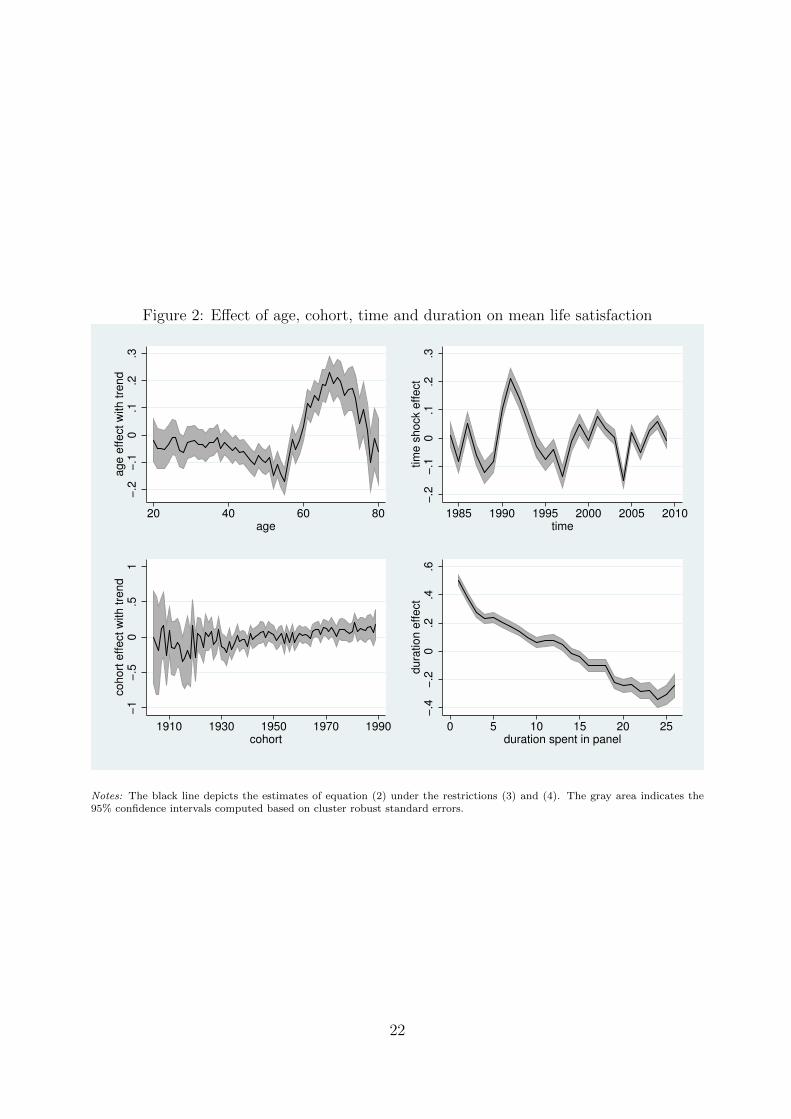
Figure 2: Effect of age, cohort, time and duration on mean life satisfaction

−.2

−.1

0.1

.2.3

ag

e e

ffe

ct

with

tre

nd

20 40 60 80age

−.2

−.1

0.1

.2.3

tim

e s

ho

ck e

ffe

ct

1985 1990 1995 2000 2005 2010time

−1

−.5

0.5

1co

ho

rt e

ffe

ct

with

tre

nd

1910 1930 1950 1970 1990cohort

−.4

−.2

0.2

.4.6

du

ratio

n e

ffe

ct

0 5 10 15 20 25duration spent in panel

Notes: The black line depicts the estimates of equation (2) under the restrictions (3) and (4). The gray area indicates the95% confidence intervals computed based on cluster robust standard errors.

22

Figure 3: Distribution of life satisfaction over the life course

0.0

5.1

20 40 60 80

Pr(y ∈ {0,1,2})

.1.1

5.2

.25

.3

20 40 60 80

Pr(y ∈ {3,4,5})

.2.2

5.3

.35

.420 40 60 80

Pr(y ∈ {6,7})

.2.2

5.3

.35

.4

20 40 60 80

Pr(y=8)

0.0

5.1

.15

.2

20 40 60 80

Pr(y=9)

0.0

5.1

.15

.2

20 40 60 80

Pr(y=10)

Notes: Results based on linear probability models. The black line depicts the estimated age effect with trend plus constant(equation (2) under restrictions (3) and (4)). The gray area indicates the 95% confidence interval computed based on clusterrobust standard errors.

23

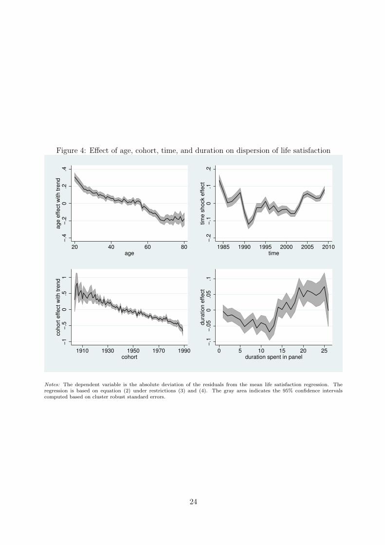
Figure 4: Effect of age, cohort, time, and duration on dispersion of life satisfaction

−.4

−.2

0.2

.4a

ge

eff

ect

with

tre

nd

20 40 60 80age

−.2

−.1

0.1

.2tim

e s

ho

ck e

ffe

ct

1985 1990 1995 2000 2005 2010time

−1

−.5

0.5

1co

ho

rt e

ffe

ct

with

tre

nd

1910 1930 1950 1970 1990cohort

−.1

−.0

50

.05

.1d

ura

tio

n e

ffe

ct


Notes: The dependent variable is the absolute deviation of the residuals from the mean life satisfaction regression. Theregression is based on equation (2) under restrictions (3) and (4). The gray area indicates the 95% confidence intervalscomputed based on cluster robust standard errors.

24

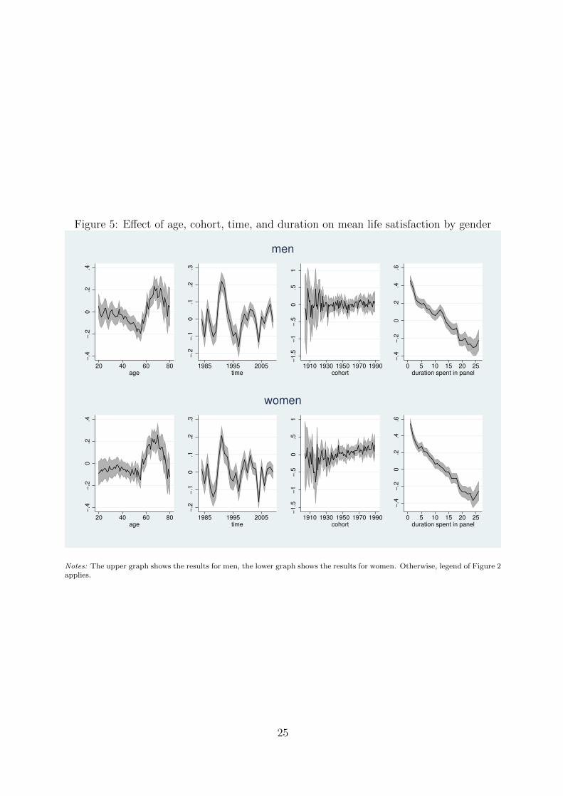
Figure 5: Effect of age, cohort, time, and duration on mean life satisfaction by gender

−.4

−.2

0.2

.4

20 40 60 80age

−.2

−.1

0.1

.2.3

1985 1995 2005time

−1

.5−

1−

.50

.51

1910 1930 1950 1970 1990cohort

−.4

−.2

0.2

.4.6


men

−.4

−.2

0.2

.4

20 40 60 80age

−.2

−.1

0.1

.2.3

1985 1995 2005time

−1

.5−

1−

.50

.51

1910 1930 1950 1970 1990cohort

−.4

−.2

0.2

.4.6


women

Notes: The upper graph shows the results for men, the lower graph shows the results for women. Otherwise, legend of Figure 2applies.

25

Figure 6: Effect of age on mean life satisfaction by education

66.5

77.5

8

20 40 60 80age

1st sextile

66.5

77.5

8

20 40 60 80age

2nd sextile

66.5

77.5

820 40 60 80

age

3rd sextile

66.5

77.5

8

20 40 60 80age

4th sextile

66.5

77.5

8

20 40 60 80age

5th sextile

66.5

77.5

8

20 40 60 80age

6th sextile

Note: The black line depicts the estimated age effect with trend (equation (2) under restrictions (3) and (4)) plus constant fordifferent education sextiles. The gray area indicates the 95% confidence interval computed based on cluster robust standarderrors.

26

Figure 7: Finite mixture model: Effect of age on mean life satisfaction

20 30 40 50 60 70 80

−0.

30−

0.20

−0.

100.

00

age

20 30 40 50 60 70 80

−0.

50.

00.

5

age

typ 1, (45%)typ 2, (32%)

typ 3, (22%)

20 30 40 50 60 70 80

−0.

4−

0.2

0.0

0.2

0.4

age

typ 1, (45%) typ 2, (55%)

20 30 40 50 60 70 80

−1.

0−

0.5

0.0

0.5

age

typ 1, (41%)typ 2, (27%)

typ 3, (16%)typ 4, (16%)

Notes: Estimated age effect on life satisfaction and estimated fraction of each class in linear finite mixture models (withnormally distributed error terms) with up to four latent classes (equation (5)).

27

Figure 8: Fraction of people reaching a minimum or maximum compared to the last ten

years

.15

.2.2

5.3

.35

fra

ctio

n

30 40 50 60 70 80age

minimum maximum

Note: The continuous (dotted) line indicates the fraction of people, who reach at this specific age the lowest (highest) lifesatisfaction level compared to the last ten years where the minimum (maximum) has not to be unique.

28

Figure 9: Distribution of observed minimums

0.0

2.0

4.0

6.0

8fr

actio

n

45 50 55 60 65age

Note: Distribution of minimums for people observing between age 48 and 62. Number of people: 979, number of minimums:2321 (minimum has not to be unique).

29

Figure 10: Distribution of evolution patterns

.1.2

.3.4

fra

ctio

n

20 40 60 80age

decreasing U−shaped

hump shaped increasing

Note: Fraction of evolution patterns between 25 and 75. In a first step, for every person and all possible intervals of lengtheleven, a simple model with two linear terms, one for the first and one for the second part, is estimated: y = β0+β1(aI(t−c−a <0)) +β2(aI(t− c−a > 0)) + ε if |t− c−a| ≤ 5, where the standard notation of the paper applies. In a second step, the resultsare classified (β1 < 0 β2 < 0 → decreasing, β1 < 0 β2 > 0 → U-shaped, β1 > 0 β2 < 0 → hump shaped, β1 > 0 β2 > 0 →increasing) and the fraction of each type is computed. Reading example: Between 30 and 40 (thus value at age 35), abouttwenty percent of the individual patterns can be described as decreasing.

30

Tables

Table 1: Summary statistics

Variable Mean Std. Dev. Min. Max.

life satisfaction 7.138 1.808 0 10

life satisfaction = 0 0.005 0 1











year 1998.0 7.6 1984 2009

age 45.6 15.7 20 80

year of education 11.5 2.6 7 18

female 0.514 0 1

cohort (year of birth) 1952.4 16.5 1904 1989

duration (year in panel) 8.0 6.2 1 26

Notes: Data from SOEP. The used sample consists of 38,197 different individuals,304,856 person-year observations, living in (former) West-Germany.

31

Table 2: Estimated trends in average life satisfaction

coeff std. err.

age + time 0.0029 (0.0011)

cohort + time 0.0029 (0.0011)

duration -0.0295 (0.0015)

constant 6.9753 (0.0180)

Observations 304,856

Individuals 38,197

Notes: The table shows the estimation resultsfor (2’). Standard errors in parentheses arecorrected for clustering at the individual level.Not shown are nonlinear components of theage profile (60 dummies), of the cohort pro-file (86 dummies), of the year profile (26 dum-mies), and of the duration profile (26 dum-mies). These are together with the trends dis-played in Figure 2.

32

soeppapers 472: heterogeneity in the relationship … in the relationship between happiness and age:...

Documents