software for multivariate outlier detection in survey · pdf filesoftware for multivariate...

SOFTWARE FOR MULTIVARIATE OUTLIERDETECTION IN SURVEY DATA

V. Todorov1 M. Templ2 P. Filzmoser3

1United Nations Industrial Development Organization (UNIDO)

2Statistics Austria

3Vienna University of Technology

Work Session on Statistical Data EditingLjubljana, Slovenia, 9-11 May 2011)

Todorov, Templ, Filzmoser (Vienna, Austria) OUTLIER DETECTION IN SURVEY DATA DATA EDIT’2011 1 / 52

Outline

1 Multivariate Outliers

2 Multivariate Location and Scatter

3 Handling of incomplete data

4 Principal Component Analysis for incomplete data

5 Summary


Multivariate Outliers

What is an Outlier

” ... whoever knows the ways of Nature will more easily notice herdeviations; and, on the other hand, whoever knows her deviations willmore accurately describe her ways.”Bacon, F. (1620) Novum OrganumHadi, Imon and Werner (2009) Detection of Outliers



What is an Outlier

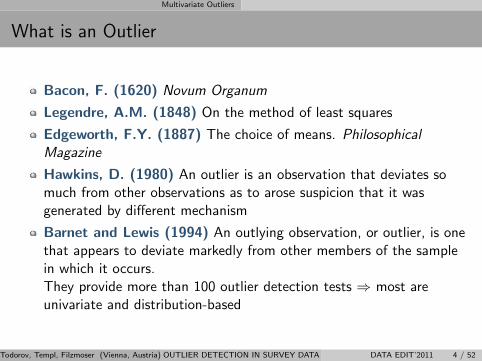
Bacon, F. (1620) Novum Organum

Legendre, A.M. (1848) On the method of least squares

Edgeworth, F.Y. (1887) The choice of means. PhilosophicalMagazine

Hawkins, D. (1980) An outlier is an observation that deviates somuch from other observations as to arose suspicion that it wasgenerated by different mechanism

Barnet and Lewis (1994) An outlying observation, or outlier, is onethat appears to deviate markedly from other members of the samplein which it occurs.They provide more than 100 outlier detection tests ⇒ most areunivariate and distribution-based



Outliers in Sample Surveys

”Rule based” approach - identification by data specific edit rulesdeveloped by subject matter experts followed by deletion andimputation ← strictly deterministic, ignore the probabilisticcomponent, extremely labor intensive

Univariate methods - favored for their simplicity. These are informalgraphical methods like histograms, box plots, dot plots; quartilemethods to create allowable range for the data; robust methods likemedians, Winsorized means, etc.

Multivariate methods - rarely used although most of the surveyscollect multivariate data



Outliers in Sample Surveys: Multivariate methods

Statistics Canada (Franklin et al., 2000) - Annual Wholesale andRetail Trade Survey (AWRTS)

Based on PCA and Stahel-Donoho estimator of multivariate locationand scatterEasily run and interpreted by the subject matter expertsLimited data set sizeOnly complete dataNo sampling weights

The EUREDIT project of the EU (Charlton 2004)

Handling of missing valuesSampling weights

Todorov, Templ and Filzmoser (2011)

Investigated and compared many different methods for detection ofmultivariate outliers based on robust estimatorsExample application to Structural Business Statistics data



Example: Bushfire data

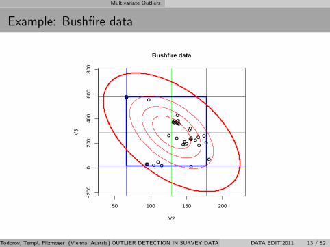
A data set with 38 observations in 5 variables - Campbell (1989)

Contains satellite measurements on five frequency bands,corresponding to each of 38 pixels

Used to locate bushfire scars

Very well studied (Maronna and Yohai, 1995; Maronna and Zamar,2002)

12 clear outliers: 33-38, 32, 7-11; 12 and 13 are suspect

Available in the R package robustbase




●●●●

●●

●●● ● ● ●

●

●

●

●●●●●●●

●

●

●● ●● ●

●

●

●●●●●●●

50 100 150 200

−20

00

200

400

600

800

Bushfire data

V2

V3




●●●●

●●

●●● ● ● ●

●

●

●

●●●●●●●

●

●

●● ●● ●

●

●

●●●●●●●

50 100 150 200

−20

00

200

400

600

800

V2

V3

Bushfire data: robust tolerance ellipse




●●●●

●●

●●● ● ● ●

●

●

●

●●●●●●●

●

●

●● ●● ●

●

●

●●●●●●●

50 100 150 200

−20

00

200

400

600

800

V2

V3





●●●●

●●

●●● ● ● ●

●

●

●

●●●●●●●

●

●

●● ●● ●

●

●

●●●●●●●

50 100 150 200

−20

00

200

400

600

800

V2

V3


33−38

710 118−9



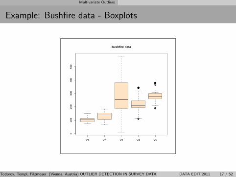
Example: Bushfire data - Boxplots

●

●●●●●●

●●

●●●●●●●

V1 V2 V3 V4 V5

010

020

030

040

050

0

bushfire data



Outliers and Robustness

Outlier detection and Robust estimation are closely related

1 Robust estimation: find an estimate which is not influenced by thepresence of outliers in the sample

2 Robustness is ”... insensitivity against small deviations from theassumptions” (Huber, 1987)

3 Outlier detection: find all outliers, which could distort the estimate

If we have a solution to the first problem we can identify the outliersusing robust residuals or distances

If we know the outliers we can remove or downweight them and useclassical estimation methods

It depends on the particular research, on which problem to set thefocus


Multivariate Location and Scatter


Location: coordinate-wise mean

Scatter: covariance matrix

Variances of the variables on the diagonalCovariance of two variables as off-diagonal elements

Optimally estimated by the sample mean and sample covariancematrix at any multivariate normal model

Essential to a number of multivariate data analysis methods

But extremely sensitive to outlying observations



MCD Estimator

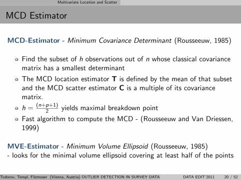
MCD-Estimator - Minimum Covariance Determinant (Rousseeuw, 1985)

Find the subset of h observations out of n whose classical covariancematrix has a smallest determinant

The MCD location estimator T is defined by the mean of that subsetand the MCD scatter estimator C is a multiple of its covariancematrix.

h = (n+p+1)2 yields maximal breakdown point

Fast algorithm to compute the MCD - (Rousseeuw and Van Driessen,1999)

MVE-Estimator - Minimum Volume Ellipsoid (Rousseeuw, 1985)- looks for the minimal volume ellipsoid covering at least half of the points



OGK Estimator

OGK-Estimator - Orthogonalized Gnanadesikan-Kettenring estimator(Maronna and Zamar, 2002; Gnanadesikan and Kettenring, 1972)

Compute robust covariance matrix pairwise byUjk = cov(Xj ,Xk) = 1

4(σ(Xj + Xk)2 − σ(Xj − Xk)2)using a robust scale as σ.

Use eigenvector/-value decomposition of U = [Ujk ] to constructrobust principal components

Obtain robust estimates of location and scatter

Not affine equivariant, but extremely fast

Other estimators - M estimator, Stahel-Donoho, S estimator,MM-estimator



Multivariate Location and Scatter: Detection ofMultivariate Outliers

Two phases (Rocke and Woodruff, 1996)

1 Calculate Robust Distances

Obtain robust estimates of location T and scatter CCalculate robust Mahalanobis-type distance

RDi =√

((xi − T)tC−1(xi − T))

2 Cutoff point: Determine separation boundary Q.

Declare points with RDi > Q, i.e. points which are sufficiently far from the robustcenter as outliers.

Usually Q = χ2p(0.975) but see also Hardin and Rocke (2005), Filzmoser, Garrett,

and Reimann (2005), Cerioli, Riani, and Atkinson (2008).



Algorithms: Handling Missing Values

Normal Imputation followed by HBDP estimation

ER-algorithm - Little (1988) ← zero breakdown point (based onM-estimates)

MCD - imputation under MVN model followed by MCD (R packagenorm and fast MCD implementation in package rrcov)

OGK - imputation under MVN model followed by OGK (fast OGKimplementation in package rrcov)

S - same as above

EM-MCD - Victoria-Feser and Copt (2004) ← cannot attain highbreakdown point

ERTBS - Victoria-Feser and Copt (2004) ← same as above




TRC - Transformed Rank Correlations - Beguin and Hulliger (2004)

EA - Epidemic Algorithm - Beguin and Hulliger (2004)

BACON-EEM - Beguin and Hulliger (2008) - a combination ofBACON algorithm (Billor, Hadi and Vellemann 2000) and EM

All three algorithms can handle sampling weights




Robust Sequential Imputation followed by HBDP estimation

SEQImpute - Sequential Imputation - Verboven et al (2007): startfrom a complete subset Xc and impute the missing values in oneobservation at a time by minimizing the determinant of theaugmented data set X∗ = [Xc ; (x∗)t ]

RSEQ - Robust Sequential Imputation - Vanden Branden andVerboven (2009): replace the sample mean and covariance by robustestimators; use the outlyingness measure proposed by Stahel (1981)and Donoho(1982)



To start with: CovNAMcd example session

R> ##

R> ## Load the 'rrcovNA' package and the data sets to be

R> ## used throughout the examples

R> ##

R> library("rrcovNA")

Scalable Robust Estimators with High Breakdown Point (version 1.2-02)

Scalable Robust Estimators with High Breakdown Point for

Incomplete Data (version 0.4-00)

R> data("bush10")



To start with: CovNAMcd example session

R> ## Compute MCD estimates for the modified bushfire data set

R> ## - show() and summary() examples

R> mcd <- CovNAMcd(bush10)

R> mcd

Call:

CovNAMcd(x = bush10)

-> Method: Minimum Covariance Determinant Estimator for incomplete data.

Robust Estimate of Location:

V1 V2 V3 V4 V5

109.5 149.5 257.9 215.0 276.9

Robust Estimate of Covariance:

V1 V2 V3 V4 V5

V1 697.6 489.3 -3305.1 -671.4 -550.5

V2 489.3 424.5 -1889.0 -333.5 -289.5

V3 -3305.1 -1889.0 18930.9 4354.2 3456.4

V4 -671.4 -333.5 4354.2 1100.1 856.0

V5 -550.5 -289.5 3456.4 856.0 671.7



Example session: summary method of CovNAMcd

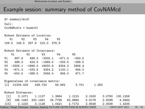
R> summary(mcd)

Call:

CovNAMcd(x = bush10)

Robust Estimate of Location:

V1 V2 V3 V4 V5

109.5 149.5 257.9 215.0 276.9

Robust Estimate of Covariance:

V1 V2 V3 V4 V5

V1 697.6 489.3 -3305.1 -671.4 -550.5

V2 489.3 424.5 -1889.0 -333.5 -289.5

V3 -3305.1 -1889.0 18930.9 4354.2 3456.4

V4 -671.4 -333.5 4354.2 1100.1 856.0

V5 -550.5 -289.5 3456.4 856.0 671.7

Eigenvalues of covariance matrix:

[1] 21334.429 428.703 56.662 3.701 1.263

Robust Distances:

[1] 3.1071 1.1127 1.3864 1.1215 2.1500 3.0780 130.1256

[8] 185.1492 200.1491 26.7795 63.9884 5.8178 2.8298 4.9464

[15] 2.1220 3.1128 1.0421 2.7172 2.9548 2.0638 1.4335

[22] 3.4786 0.1621 1.2949 1.0765 1.0287 2.5304 0.7860

[29] 3.4224 5.8211 151.4576 435.4440 238.2627 69.9555 323.5308

[36] 322.8153 312.4068 235.6941



Example session: plot method of CovNAMcd

R> plot(mcd)

0.5 1.0 1.5 2.0 2.5 3.0 3.5

05

1015

20

Mahalanobis distance

Rob

ust d

ista

nce

●

●●●●

●

●

●●

●

●

●

●●

●●

●●●

●●

●

●

●●●●

●

●●

●

●

●

●

●●●

●

10

1134

731

89

3833

373635

32

Distance−Distance Plot



A propos - R Graphics

R offers three main types of graphics: traditional (or base), lattice,and ggplot2. The latter two have as underlying graphics system thegrid package.

The base graphics functions come with the main R installation andinclude high-level functions such as bar plots, histograms, and scatterplots - brief, with good default settings; Also include low-level functionsfor drawing points, lines, axes, etc which add flexibility and control forcreating new types of graphs. Paul Murrell (2005)The lattice graphics package, written by Deepayan Sarkar implementsW. S. Cleveland’s Trellis graphics system and now is part of the base Rdistribution. Deepayan Sarkar (2007)The third graphics package, ggplot2, written by Hadley Wickham, isbased on the grammar of graphics and offers an excellent balancebetween power and ease of use. Hadley Wickham (2009)

All plots in rrcov are implemented in base graphics but many plotshave already lattice alternatives



Example session: more plots for CovNAMcd: distance plot

R> plot(mcd, which="xydistance")

Distance Plot

Index

Mah

alan

obis

dis

tanc

e

0

5

10

15

20

0 10 20 30

●

●●●●

●

●

●●

●

●

●

●●

●●

●

●●●

●

●

●

●●●●

●

●●

●

●

●

●

●●●

●

10

11 34

731

89

3833

373635

32Robust

0 10 20 30

●

●

●●

●

●

●●●

●●●●

●●●

●●

●●●

●

●●

●●●

●●

●●●

●●●●●●

7

Classical The robust distances areplotted versus their index -the outliers have large RDi

A line is drawn aty = cutoff =

√χ2

p,0.975

The observations withMDi ≥ cutoff =

√χ2

p,0.975

are identified by their index

The observations which havea missing value in any of thecoordinates are shown in red.



Example session: more plots ... χ2 QQ-plot

R> plot(mcd, which="xyqqchi2")

χ2 QQ−Plot

Sqrt of the quantiles of the χ2 distribution

Mah

alan

obis

dis

tanc

e

0

5

10

15

20

1.0 1.5 2.0 2.5 3.0 3.5

●● ●●●●●●●●●

●●●●●●●●●●●

●●●

●

●●

●

●

●●

●●

●● ●

●

10

1134

731

89

3833

373635

32

Robust

1.0 1.5 2.0 2.5 3.0 3.5

●● ●●●●●●●●●●●●●

●●●●●●●●●●●●●●●●●●●●

● ● ●7

Classical

A Quantile-Quantilecomparison plot of theRobust distances and theMahalanobis distances versusthe square root of thequantiles of the chi-squareddistribution

The observations which havea missing value in any of thecoordinates are shown in red.



Example session: more plots ... tolerance ellipses

R> mcd2 <- CovNAMcd(bush10[,2:3])

R> plot(mcd2, which="tolEllipse", class=TRUE)

50 100 150 200

−20

00

200

400

600

800

89

373635

Tolerance ellipse (97.5%)

● robustclassical

●● ●●

●●

●●● ● ● ●

●

●

●

●●●●●

●●

●

●

●

●

●

●

●

●

●

●

●

● ●●●

●

Consider the case of bivariatedata (variables V2 and V3 ofbush10 data set) - see nextslide for more than twovariables

Scatter plot of the data withsuperimposed 97.5% robustand classical tolerance ellipses

The observations withMDi ≥ cutoff =

√χ2

p,0.975

are identified by theirsubscript

The observations which havea missing value in any of thecoordinates are projected onthe axis and are shown in red.



Example session: more plots ... pairs

R> plot(mcd, which="pairs")

V1

80 120 180

●●

●

●●

●●●●●

● ● ●

●

●●●●●●●●

●●

●●●●

●

●●

●

●● ●●●●

●●

●

●●●●●●

●

●●●

●

●●●●●●●●

●●

●●●●

●

●●

●

● ●●●●●

150 250 350

●●

●

●●●●●●●

●● ●

●

●●●●●●●●

●●●●●●

●

●●

●

●●●● ●●

8011

014

0

●●

●

●●●●●●●

●●●

●

●●●●●●●●

●●●●●●

●

●●

●

●●● ●●●

8012

018

0

(0.77)0.90

V2●

●

●●●●

●●●●●

●

●

●●●●●●●●●

●●

●● ●● ●●●

●

●

●

●●●●

●

●

●●●●

●●●

●●

●

●

●●●●●●●●●

●●●●●●● ●

●

●

●

●

●● ●●

●

●

●●●●

●●●

●●

●

●

●●●●●●●●●

●●●●●●●●

●

●

●

●

● ●●●

(−0.48)

−0.91

(−0.35)

−0.67

V3●●●● ●●

●●●● ●●●

●

●●●●●●●●

●

●●

●

●

●

●

●

●

●

●

●●● ●

● 020

050

0

●●●●●●

●●●●●●●

●

●●●●●●●●

●

●●

●

●

●

●

●

●

●

●

●● ●●

●

150

250

350

(−0.45)

−0.77

(−0.47)

−0.49

(0.97)0.95

V4●●●

●

●●●

●●

●

●

●

●●

●●●●●●●●●●●●●●

●

●●

●●●●

●

●●

80 110 140

(−0.43)

−0.80

(−0.41)

−0.54

0 200 400

(0.97)0.97

(1.00)1.00

200 300

200

300

V5



Example session: more plots ... screeplot

R> data(ces)

R> plot(CovNAMcd(ces), which="screeplot")

1 2 3 4 5 6 7 8

0e+

001e

+08

2e+

083e

+08

4e+

08

Index

Eig

enva

lues

● robustclassical

●

● ● ● ● ● ● ●

Scree plot

Robust and classical Screeplot of the data

Eigenvalues comparison plotfor the ConsumerExpenditure Survey Data -Hubert et al. (2009).

Find out if there is muchdifference between theclassical and robustcovariance (or correlation)estimates.


Handling of incomplete data

Handling of incomplete data in - package rrcovNA

CovNAMcd - Minimum Covariance Determinantno imputation: Victoria-Feser and Copt (2004) ornormal imputation orrobust sequential imputation or”other” robust imputation

CovNAOgk - Pairwise cov estimatorsame imputation methods as in CovNAMcd

CovNASest - S estimatessame imputation methods as in CovNAMcdseveral estimation methods FAST S, SURREAL, Bisquare, Rocke type

CovNASde - Stahel-Donoho estimatorsame imputation methods as in CovNAMcd

CovNABacon - BACON-EEM algorithm as described in Beguin andHulliger (2008)

PcaNA - Different robust PCA methos for incomplete data - seeSerneels (2008) - to be discussed later in this presentation.



CovNARobust: a generalized function for robust locationand covariance estimation for incomplete data - packagerrcovNA

CovNARobust(x, control, na.action = na.fail)

Computes a robust multivariate location and scatter estimate with ahigh breakdown point, using one of the available estimators.

Select the estimation method through the argument control. It canbe:

A control object with estimation options, e.g. an object of classCovControlMcd signals MCD estimationA character string naming the desired method, like ”mcd”,”ogk”, etc.Empty - than the function will select a method based on the size of theproblem

Demonstrates the power of the OO paradigm - the function is shorterthan half screen and has no switch on the method



CovRobust(): example

R> getMeth(CovNARobust(matrix(rnorm(40),ncol=2)))

[1] "Stahel-Donoho estimator"


[1] "S-estimates: bisquare"


[1] "S-estimates: Rocke type"

R> getMeth(CovNARobust(matrix(rnorm(2E5),ncol=2)))

[1] "Orthogonalized Gnanadesikan-Kettenring Estimator"


Principal Component Analysis for incomplete data

Principal Component Analysis

Data matrix X with n rows (observations) and p columns (variables)

Goal: Dimension reduction - the information contained in themultivariate data should be expressed by few components withminimal loss of information.

Solution: Spectral decomposition of the covariance matrix of X:

Σ=ΓΛΓt

The (estimated) principal components:

Z=(X-1µ) Γ

Estimates (arithmetic mean and sample covariance matrix)

µ = x and Σ=S



Example: Principal Component Analysis

A bivariate data set with: n = 60, µ = (0, 0) and ρ = 0.8

sample correlation: 0.84

sort the data by the first coordinate x1 and modify the first fourobservations with smallest x1 and the last four with largest x1 byinterchanging their first coordinates

thus (less than) 15% of outliers are introduced which areundistinguishable on the univariate plots of the data

the sample correlation changes even its sign and becomes -0.05


●●

●● ●

●

●

●

●

●●

●

●

●●

●

●

●

●

●

●

●

●

●

●

●

●

●

●

●● ●

●

●

●

●

●

●●

●

●

●●

●

●●

●●

●●

●● ●

●●

●

●

● ●●

−4 −2 0 2 4

−4

−2

02

4

(a) Clean data

x1

x 2

PC1

●●

●● ●

●

●

●

●

●●

●

●

●●

●

●

●

●

●

●

●

●

●

●

●

●

●

●

●● ●

●

●

●

●

●

●●

●

●

●●

●

●●

●●

●●

●● ●

●●

●

●

● ●●

−4 −2 0 2 4

−4

−2

02

4

(b) Data with 15% outliers

x1

x 2

PC1

●●

●● ●

●

●

●

●●●

●

●

●●

●

●

●

●

●

●

●

●

●

●

●

●

●

●

●

● ●

●

●

●

●

●

●

●

●

●

●

●

●

●

●

●

●

●

●

●

●

●

●●

●

●

●●

●

−3 −2 −1 0 1 2 3

−2

−1

01

2

(c) Classical

PC1

PC

2

●

●

●

●●

●

●

●

●

●●

●

●

●●

●●

●●

●

●

●

●

●

●

●

●● ●

● ●

●

●

●

●

●

●

●

●● ●

●

● ●

●

●

●

●● ●●

●

●

●●●

●

●

●

●

−2 0 2

−3

−1

01

23

(d) Robust (MCD)

PC1

PC

2


Principal Component Analysis for Incomplete data

Walczak and Massart (2001) - use the EM approach applied toclassical PCA.

Serneels and Verdonck (2008) - use the EM approach applied toany robust PCA.

Most of the available robust PCA methods are implemented in the Rpackage rrcov

The corresponding methods for dealing with incomplete data areavailable in the package rrcovNA



Principal Component Analysis for Incomplete data

PcaNA(x, k, method, cov.control, ...)

PcaNA(formula, data = NULL, ...)

method=”cov” - PCA based on a robust covariance matrix. Differentestimators of the covariance matrix can be used.

method=”proj” - Projection pursuit approach (Croux andRuiz-Gazen, 1996, 2005)

method=”grid” - Projection pursuit approach, enhanced searchalgorithm (Croux, Filzmoser, Oliveira, 2007)

method=”hubert” - ROBPCA, (Hubert, Rousseeuw and VandenBranden, 2005)

method=”locantore” - Spherical PCA (Locantore et al., 1999)

method=”class” - Classical PCA.



Example session: PcaNA

R> data(bush10)

R> pca <- PcaNA(bush10) # by default the MCD cov matrix will be used

R> pca

Call:

PcaNA.default(x = bush10)

Standard deviations:

[1] 145.627942 21.836183 10.869330 3.366705 1.574500

Loadings:

PC1 PC2 PC3 PC4 PC5

V1 -0.1472945 0.2971574 0.4885216 0.80001612 -0.10640793

V2 -0.1015296 0.4235344 0.6815787 -0.57745246 0.11094823

V3 0.9573892 -0.1098694 0.2607165 0.05576422 -0.01587048

V4 0.1762042 0.6946248 -0.3738399 -0.07496570 -0.58401396

V5 0.1426675 0.4875872 -0.2984421 0.13339174 0.79689627



Example session: PcaNA

R> pca <- PcaNA(bush10, cov.control=CovControlSde()) # use SDE

R> pca

Call:

PcaNA.default(x = bush10, cov.control = CovControlSde())

Standard deviations:

[1] 167.012473 18.768804 11.356572 3.869779 1.389190

Loadings:

PC1 PC2 PC3 PC4 PC5

V1 -0.13638664 0.2524196 0.4289942 0.85133076 -0.09424951

V2 -0.08679023 0.6449877 0.5753147 -0.48267359 0.11179214

V3 0.95054687 -0.1030613 0.2906412 0.03509577 -0.01161905

V4 0.20871804 0.6031312 -0.4970402 0.04013959 -0.58652306

V5 0.16359576 0.3819506 -0.3917342 0.19854281 0.79653954



Example session: summary method of PcaNA

R> summary(pca)

Call:

PcaNA.default(x = bush10, cov.control = CovControlSde())

Importance of components:

PC1 PC2 PC3 PC4 PC5

Standard deviation 167.0125 18.76880 11.35657 3.86978 1.38919

Proportion of Variance 0.9825 0.01241 0.00454 0.00053 0.00007

Cumulative Proportion 0.9825 0.99486 0.99940 0.99993 1.00000



Example session: plot method of PcaNA

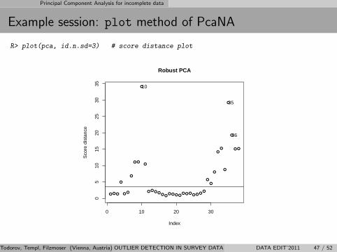
R> plot(pca, id.n.sd=3) # score distance plot

● ● ●

●

● ●

●

● ●

●

●

● ● ● ●● ●

● ● ● ●● ● ●

● ● ●●

●

●

●

●●

●

●

●

● ●

0 10 20 30

05

1015

2025

3035

Index

Sco

re d

ista

nce

36

35

10

Robust PCA



Example session: plot method of PcaNA

R> ## Score distance plot for the fish data set

R> data(fish); ## obs. 14 has a missing value

R> plot(PcaNA(fish[,1:6]), col=fish[,7]+1, pch=fish[,7]+10, id.n.sd=0)

●

●●

●

●

●

●

●

●

●●

●●●

●●

●

●

●●

●●●

●

●

●

●●

●

●●●●●

●●

●

0 50 100 150

02

46

810

12

Index

Sco

re d

ista

nce

Robust PCA



Score distances and orthogonal distances

An outlier in the context of PCA is characterized by the following:

Lies far from the subspace spanned by the first k eigenvectors (largeorthogonal distance) and/orThe projected observation lies far from the bulk of the data within thisspace (large score distance)

The score distances are given by:

SDi =

√∑kj=1

t2ij

lj, i = 1, . . . , n

where lj are the eigenvalues

The orthogonal distances of each observation to the subspacespanned by the first k principal components are defined by:ODi = ||xi − µi − Pti || , i = 1, . . . , n



Outlier map (Hubert et al, 2005)

R> opar <- par(mfrow=c(1,2))

R> plot(PcaNA(bush10,k=2, method="class"), main="Classical PCA")

R> plot(PcaNA(bush10,k=2, method="hubert"), main="Robust PCA")

R> par(opar)

● ●●●

●

●

●

●

●

●

●

● ●

●

●

●

●●●●

●●

●

●

●

●●

●

●

●●

●

●

● ●●

●

●

0.0 0.5 1.0 1.5 2.0 2.5

010

2030

40

Classical PCA

Score distance

Ort

hogo

nal d

ista

nce

13 7

15

10

89

●

●

●

●●

●

●

●●

●

●

●

●● ●●●●●●●●

●●

● ●●

●●

●●

●

●●

●●

●●

0.0 0.5 1.0 1.5 2.0 2.5

020

6010

0

Robust PCA

Score distance

Ort

hogo

nal d

ista

nce

89

11

38

710


Summary

Summary and Conclusions

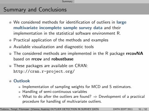
We considered methods for identification of outliers in largemultivariate incomplete sample survey data and theirimplementation in the statistical software environment R.

Practical application of the methods and examples

Available visualization and diagnostic tools

The considered methods are implemented in the R package rrcovNAbased on rrcov and robustbase

These packages are available on CRAN:http://cran.r-project.org/

OutlookImplementation of sampling weights for MCD and S estimators.Handling of semi-continuous variablesWhat to do after the outliers are found? ⇒ Development of a practicalprocedure for handling of multivariate outliers.


http://cran.r-project.org/

Summary

References I

V. Todorov, M.Templ and P. FilzmoserDetection of multivariate outliers in business survey data withincomplete information,Advances in Data Analysis and Classification, 5, 37–56, 2011

V. Todorov and P. FilzmoserAn object oriented framework for robust multivariate analysis,Journal of Statistical Software, 32(3), 1–47, 2009http://www.jstatsoft.org/v32/i03/

M. Hubert, P.J. Rousseeuw and S. van AelstHigh-Breakdown Robust Multivariate Methods,Statistical Science, 23, 92–119, 2008.


http://www.jstatsoft.org/v32/i03/

software for multivariate outlier detection in survey · pdf filesoftware for multivariate...

Documents