software reliability: a preliminary handbook · software reliability: a preliminary handbook ......
TRANSCRIPT

Software Reliability:A Preliminary Handbook
PUBLICATION NO. FHWA-RD-04-080 SEPTEMBER 2004
Research, Development, and TechnologyTurner-Fairbank Highway Research Center6300 Georgetown PikeMcLean, VA 22101-2296

FOREWORD A goal of the Federal Highway Administration’s (FHWA) Advanced Safety Research Program is to help highway engineers, software developers, and project mangers understand software verification and validation (V&V) and produce reliable, safe software. This handbook presents new software V&V techniques to address special needs related to highway software. Some of the techniques are:
• Wrapping (using embedded code to make a program self-verifying).
• SpecChek™, a V&V tool to check software with its specifications.
• Real-time computation of error propagation.
• Phased introduction of new software to minimize failures. The results of this research will be useful to transportation engineers, software managers and developers, and safety professionals who are involved in creating highway-related software. Michael F. Trentacoste Director, Office of Safety Research, and Development
NOTICE This document is disseminated under the sponsorship of the U.S. Department of Transportation in the interest of information exchange. The U.S. Government assumes no liability for its contents or use thereof. This report does not constitute a standard, specification, or regulation. The U.S. Government does not endorse products or manufacturers. Trade and manufacturers’ names appear in this report only because they are considered essential to the object of this document.
QUALITY ASSURANCE STATEMENT
FHWA provides high-quality information to serve Government, industry, and the public in a manner that promotes public understanding. Standards and policies are used to ensure and maximize the quality, objectivity, utility, and integrity of its information. FHWA periodically reviews quality issues and adjusts its programs and processes to ensure continuous quality improvement.

1. Report No. FHWA-HRT-04-080
2. Government Accession No.
3. Recipient’s Catalog No. 5. Report Date September 2004
4. Title and Subtitle Software Reliability: A Preliminary Handbook 6. Performing Organization Code
7. Author(s) Rodger Knaus, Hamid Aougab, Naim Bentahar
8. Performing Organization Report No. 10. Work Unit No.
9. Performing Organization Name and Address Instant Recall, Inc. 8180 Greensboro Drive, Suite 700 McLean, VA 22102 www.irecall.com
11. Contract or Grant No. FHWA-RD-DTFH61-02-F-00154
13. Type of Report and Period Covered
12. Sponsoring Agency Name and Address Office of Safety Research and Development Federal Highway Administration 6300 Georgetown Pike McLean, VA 22101-2296
14. Sponsoring Agency Code
15. Supplementary Notes COTR: Milton Mills, Office of Safety Research and Development
16. Abstract The overall objective of this handbook is to provide a reference to aid the highway engineer, software developer, and project manager in software verification and validation (V&V), and in producing reliable software. Specifically, the handbook: • Demonstrates the need for V&V of highway-related software. • Introduces the important software V&V concepts. • Defines the special V&V problems for highway-related software. • Provides a reference to several new software V&V techniques developed under this and earlier related projects to
address the special needs of highway-related software: o Wrapping, i.e., the use of embedded code to make a program self-verifying. o SpecChek™, a V&V tool to check software with its specifications. o Real-time computation of roundoff and other numerical errors. o Phased introduction of new software to minimize failures.
• Helps the highway engineer, software developer, and project manager integrate software V&V into the development of new software and retrofit V&V into existing software.
The handbook emphasizes techniques that address the special needs of highway software, and provides pointers to information on standard V&V tools and techniques of the software industry. 17. Key Words Software Reliability, Roundoff Errors, Floating Points Errors, Software Verification and Validation, Software Testing, SpecChek
18. Distribution Statement No restrictions. This document is available to the public through the National Technical Information Service, Springfield, VA 22161.
19. Security Classif. (of this report) Unclassified
20. Security Classif. (of this page) Unclassified
21. No. of Pages 85
22. Price

ii
SI* (MODERN METRIC) CONVERSION FACTORS APPROXIMATE CONVERSIONS TO SI UNITS
Symbol When You Know Multiply By To Find Symbol LENGTH
in inches 25.4 millimeters mm ft feet 0.305 meters m yd yards 0.914 meters m mi miles 1.61 kilometers km
AREA in2 square inches 645.2 square millimeters mm2
ft2 square feet 0.093 square meters m2
yd2 square yard 0.836 square meters m2
ac acres 0.405 hectares ha mi2 square miles 2.59 square kilometers km2
VOLUME fl oz fluid ounces 29.57 milliliters mL gal gallons 3.785 liters L ft3 cubic feet 0.028 cubic meters m3
yd3 cubic yards 0.765 cubic meters m3
NOTE: volumes greater than 1000 L shall be shown in m3
MASS oz ounces 28.35 grams glb pounds 0.454 kilograms kgT short tons (2000 lb) 0.907 megagrams (or "metric ton") Mg (or "t")
TEMPERATURE (exact degrees) oF Fahrenheit 5 (F-32)/9 Celsius oC
or (F-32)/1.8 ILLUMINATION
fc foot-candles 10.76 lux lx fl foot-Lamberts 3.426 candela/m2 cd/m2
FORCE and PRESSURE or STRESS lbf poundforce 4.45 newtons N lbf/in2 poundforce per square inch 6.89 kilopascals kPa
APPROXIMATE CONVERSIONS FROM SI UNITS Symbol When You Know Multiply By To Find Symbol
LENGTHmm millimeters 0.039 inches in m meters 3.28 feet ft m meters 1.09 yards yd km kilometers 0.621 miles mi
AREA mm2 square millimeters 0.0016 square inches in2
m2 square meters 10.764 square feet ft2
m2 square meters 1.195 square yards yd2
ha hectares 2.47 acres ac km2 square kilometers 0.386 square miles mi2
VOLUME mL milliliters 0.034 fluid ounces fl oz L liters 0.264 gallons gal m3 cubic meters 35.314 cubic feet ft3
m3 cubic meters 1.307 cubic yards yd3
MASS g grams 0.035 ounces ozkg kilograms 2.202 pounds lbMg (or "t") megagrams (or "metric ton") 1.103 short tons (2000 lb) T
TEMPERATURE (exact degrees) oC Celsius 1.8C+32 Fahrenheit oF
ILLUMINATION lx lux 0.0929 foot-candles fc cd/m2 candela/m2 0.2919 foot-Lamberts fl
FORCE and PRESSURE or STRESS N newtons 0.225 poundforce lbf kPa kilopascals 0.145 poundforce per square inch lbf/in2
*SI is the symbol for th International System of Units. Appropriate rounding should be made to comply with Section 4 of ASTM E380. e(Revised March 2003)

iii
Table of Contents
Introduction............................................................................................................................... 1 Scope and Purpose of This Handbook .......................................................................................................1 The Need for Software V&V in Highway Engineering ............................................................................1 Definitions of Correctness Criteria ..............................................................................................................2 Overview of V&V Techniques .....................................................................................................................3 Special V&V Requirements of Highway Engineering Software ..............................................................4 Organization of Handbook ...........................................................................................................................5
Software Life Cycle ....................................................................................................................7 Software Development Life Cycles (SDLC)...............................................................................................7 Software Development Phases .....................................................................................................................8 Scope of Chapter ............................................................................................................................................8 What Constitutes Testing ..............................................................................................................................9
Software Testing...................................................................................................................... 11 Definition of Software Testing ...................................................................................................................11 Why Test?.......................................................................................................................................................11 Scope of Chapter ..........................................................................................................................................11 What Constitutes Testing ............................................................................................................................12 What to Include in the Test Sample...........................................................................................................12 How to Select the Test Sample...................................................................................................................13 How Many Inputs Should Be Tested.........................................................................................................13 Limitations of Testing ..................................................................................................................................14
Safe Introduction of Software Using Scale Up........................................................................ 15 The Problem..................................................................................................................................................15 What Is Learned from “n” Successes ........................................................................................................15 Extensions......................................................................................................................................................17 Applications ...................................................................................................................................................17 Conclusion .....................................................................................................................................................19
Informal Proofs........................................................................................................................ 21 Introduction...................................................................................................................................................21 Simple Examples...........................................................................................................................................21 Advantages and Limitations of Informal Proofs .....................................................................................23 Symbolic Evaluation.....................................................................................................................................24 Using a Proof in V&V..................................................................................................................................30
Wrapping ................................................................................................................................. 31 Introduction...................................................................................................................................................31

iv
The Matrix Inverse .......................................................................................................................................32 Wrapping the Integer Factorial ...................................................................................................................34 Limitations of Wrapping..............................................................................................................................37 Wrapping with Executable Specifications.................................................................................................37 Knowledge Representation of Specifications ...........................................................................................38 Translating Informal Specifications into Decision Trees........................................................................40 Partial Translation Transformations ..........................................................................................................40 SpecChek........................................................................................................................................................42 SpecChek’s Own Reliability.........................................................................................................................47 Using SpecChek in the Software Life Cycle..............................................................................................48 Advantages of SpecChek for Wrapping ....................................................................................................48 An Example ...................................................................................................................................................49
Numerical Reliability ..............................................................................................................53 Framework Reference ..................................................................................................................................53 Errors in a Single Arithmetic Operation ...................................................................................................53 Computing Errors for an Entire Computation ........................................................................................63
Tools for Software Reliability ..................................................................................................65 Resources .......................................................................................................................................................65 Tools ...............................................................................................................................................................66
Appendix A. Wrapping Source Code.......................................................................................67 Run of Integer Factorial...............................................................................................................................67 Run of Wrapped Factorial ...........................................................................................................................68
Appendix B. Roundoff Errors in Large Sum...........................................................................69 Errors in the Sum of a List of Numbers ...................................................................................................69 Averrdemo.c ..................................................................................................................................................72 Random Quotients .......................................................................................................................................74
References................................................................................................................................77 Additional Resources.......................................................................................................................... 79

v
List of Figures Figure 1: The V (U) Model for SDLC ....................................................................................................................... 9 Figure 2: Simplified V Model with Handbook Techniques ................................................................................10 Figure 3: Model of SpecChek Method.....................................................................................................................43 Figure 4: Checking Software with SpecChek..........................................................................................................44

vi
List of Tables Table 1: Formula for Addition...................................................................................................................................57 Table 2: Formula for Subtraction..............................................................................................................................58 Table 3: Formula for Multiplication .........................................................................................................................61 Table 4: Formula for Division ...................................................................................................................................62 Table 5: Order Errors for Addition..........................................................................................................................70

1
Chapter 1 Introduction
Scope and Purpose of This Handbook
The overall objective of this handbook is to provide a reference to aid highway engineers, software developers, and project managers in software verification and validation (V&V), and in producing reliable software. Specifically, the handbook:
• Demonstrates the need for V&V of highway-related software.
• Introduces the important software V&V concepts.
• Defines the special V&V problems for highway-related software.
• Provides a reference to several new software V&V techniques developed under this and earlier related projects to address the special needs of highway-related software:
o Wrapping, i.e., the use of embedded code to make a program self-verifying. o SpecChek™, a V&V tool to check software with its specifications o Real-time computation of roundoff and other numerical errors.
o Phased introduction of new software to minimize failures.
• Helps highway engineers, software developers, and project managers integrate software V&V into the development of new software and retrofit V&V into existing software.
The handbook emphasizes techniques that address the special needs of highway software and provides information on standard V&V tools and techniques of the software industry.
Current Status: The scope of the project to produce this handbook was not large enough to address many of the problems involving software that were uncovered along the way. A decision was made to concentrate on wrapping and estimating numerical errors, because these seemed important, widely applicable, not adequately addressed in the available literature, and tractable.
Intended Audience: Some mathematical and computer programming experience is assumed for this handbook, especially the chapters relating to informal proofs, scale up, and estimation of numerical errors.
The Need for Software V&V in Highway Engineering
Software development is a relatively new activity used by an ancient profession. Construction and roadway engineering began in prehistoric times, and over time, the industry has raised the standards in design,

2
construction, practice documentation. Through modernizing and improving design, construction, and maintenance, new approaches and technologies have been incorporated into civil engineering practice.
Many of the new tools and technologies initially did not achieve the levels of reliability and standardization that the civil engineering profession demanded; software development and computer programs fall into this category.
Software planning and development should emulate construction project planning, design, and construction, integrating testing and evaluation. The end result will be more reliable software and transportation systems.
Software developers must use tools to improve software and catch design problems at an early stage of the software development life cycle, when fixing these problems is relatively inexpensive and easy. These tools must be easy to use for both the software designer and for the software developer, and not just for those with unusual mathematical training.
In traditional software engineering, developers claim that testing is an integral part of the design and development process. However, as programming techniques become more advanced and complex, there is little consensus on what testing is necessary or how to perform it. Furthermore, many of the procedures that have been developed for V&V are so poorly documented that only the originator can reproduce the procedures. The complexity and uncertainty of these procedures has led to the inadequate testing of software systems (even operational systems). As software becomes more complex, it becomes more difficult to produce correct software, and the penalties for errors will increase.
Definitions of Correctness Criteria
V&V is the traditional terminology for the process of ensuring that software performs as required for its intended task. Verification is the process of checking that the software meets its specifications, i.e., that the software was built correctly. Validation is the process of checking that the software performs properly when used, i.e., that the correct software was built.
The V&V approach to software correctness assumes that good specifications exist. As discussed below, specifications for highway software often evolve over time. Therefore, this handbook has expanded the traditional concept of V&V to include the preparation, maintenance, and use of good specifications.
Software reliability is “the probability of failure-free operation of a computer program for a specified time in a specified environment.”(1)
The study of software reliability often emphasizes predicting software failures. As Leveson observes, not all failures are important for software safety.(2) In addition, predicting failures is less important than finding and fixing failures. For these reasons, predicting failure as an end in itself will not be emphasized in this handbook.

3
Software correctness is a set of criteria that defines when software is suitable for engineering applications that:(3)
• Compute accurate results.
• Operate safely, and cause the system that contains the software to operate safely.
• Perform the tasks required by the system that contains the software, as explained in the software specifications.
• Achieve these goals for all inputs.
• Recognize inputs outside the domain.
Software correctness is a broad definition of what it means for software to perform correctly. Because it emphasizes accuracy, safety, and acceptable operation of a system containing software, software correctness is a useful concept by which to judge highway-related software.
Overview of V&V Techniques
Categories of V&V Techniques
In an extensive catalog of V&V techniques, Wallace et al. divide V&V techniques into three categories.(4)
• Static analysis techniques are “those which directly analyze the form and structure of a product without executing the product. Reviews, inspections, audits, and data flow analysis are examples of static analysis techniques.”
• Dynamic analysis techniques “involve execution, or simulation, of a development activity product to detect errors by analyzing the response of a product to sets of input data. Testing is the most frequent dynamic analysis technique.”
• Formal analysis (or formal methods) “is the use of rigorous mathematical techniques to analyze the algorithms of a solution. Sometimes the software requirements may be written in a formal specification language (e.g., Z (see The World Wide Web Virtual Library: the Z Notation http://vl.zuser.org) which can be verified using a formal analysis technique like proof-of-correctness.”
Important Techniques for Highway Software
Here are short definitions of some V&V techniques that are important for use on highway software. These techniques are discussed more extensively in later chapters of the handbook.
Testing: The process of experimentally verifying that a program operates correctly. It consists of:
4
1. Running a sample of input data through the target program.
2. Checking the output against the predicted output.
Wrapping: The inclusion of code that checks a software module in the module itself, and reports success or failure to the module caller.
To make wrapping practical for engineering problems, a simple form of executable specifications has been developed, along with software for executing the specifications.
Informal Proofs: Mathematical proofs at about the level of rigor of engineering applications of calculus. These proofs establish mathematical properties of the abstract algorithm expressed by a computer program.
Numerical Error Estimation: A technique is provided for estimating the numerical error in a computation due to measurement errors of the inputs, numerical instabilities, and roundoff errors during the computation.
Excluded Techniques
In choosing methods to highlight in the handbook, the goal has been to improve current practice. Therefore, techniques that are in widespread current use, such as dataflow diagrams, have not been included. Another reason for leaving out many of the static techniques is that, in contrast to practice in other engineering fields, the static methods do not examine the final work product with either theory or experiment.
In addition, methods for which writing the specifications in a formal specification language is at least as difficult as writing the software itself have been excluded, because these methods are judged to be too expensive, too error-prone, and too foreign to current practitioners to be practical.
Special V&V Requirements of Highway Engineering Software
Evolving Specifications
Applying traditional software V&V techniques to highway software is particularly difficult because the specifications for that software are usually complex and incomplete. This is because software like CORSIM (a tool that simulates traffic and traffic control conditions on combined surface streets and freeway networks) models real-world systems that have complex, often conflicting requirements placed on them. In addition, the long life and wide application of some highway software means that the original software specifications cannot anticipate all the tasks the software will be asked to perform during its lifetime. The traditional specify-develop-validate life cycle is not completely practical in the real world. Accordingly, the techniques presented in this handbook are designed to fit into a real-world situation in which a program and its specifications evolve over time. The wrapping technique and accompanying SpecChek tool have been provided to meet this need.

5
Correctness of Numerical Computations
Many complex numerical computations occur in highway engineering, such as large finite-element calculations and complex simulations. These large calculations use numerical algorithms such as matrix inversion, numerical integration, and relaxation solution of differential equations that are known to generate errors. Numerical errors and instabilities due to the finite precision of computer arithmetic are hard to detect if they occur deep in these computations. Therefore, a method for computing an approximate error along with numerical results has been developed so that error estimates can be pushed through a computation. Using this method, it is possible to determine whether a numerical calculation contains numerical errors.
Safety Critical Software Applications
Many software applications in highway engineering are safety critical. Some highway software, such as collision avoidance software in intelligent transportation systems (ITS), will be run millions of times under a wide variety of conditions. If a bug exists, these conditions are likely to expose it. Consequently, a very high standard of software reliability is required for safety-critical highway software.
Organization of Handbook
Chapter 1, “Introduction” (this chapter) introduces V&V terminology, discusses the special problems of V&V for highway software, and outlines handbook contents.
Chapter 2, “Testing,” discusses what is learned about software from testing, criteria for choosing test cases, and practical testing limitations.
Chapter 3, “Safe Introduction of Software Using Scale Up,” explains how software can be introduced in its environment using scale up.
Chapter 4, “Informal Proofs,” defines a framework for informal proofs about programs, introduces proof techniques for informal proofs, and discusses applications. It contains simple examples of informal proofs and lists their limitations.
Chapter 5, “Wrapping,” explains how verification code within a program can make the program self-testing, documents how to use executable specifications to implement wrapping for highway software and discusses a sample highway application. It outlines the benefits and limitations to wrapping.
Chapter 6, “Estimating Numerical Errors,” explains a method for computing the expected numerical errors in a numerical computation.
Chapter 7, “Information Sources and Tools,” lists some of the most important sources of information about V&V and some available tools that can help achieve software correctness.


7
Chapter 2 Software Life Cycle
The techniques developed in this handbook can be applied separately or in conjunction to improve the reliability of the software product. This chapter examines the utilization of these techniques throughout the software development life cycle.
This chapter discusses:
• Software development life cycles.
• Software development phases.
• Application of the handbook’s techniques in the life cycle.
Software Development Life Cycles (SDLC)
When developing any large complex system, it is customary to divide it into tasks or groups of related tasks that make it easy to understand, organize, and manage. In the context of software projects, these tasks or groups of tasks are referred to as phases. Grouping these phases and their outcomes in a way that produces a software product is called a software process or an SDLC.
There are many different software processes, and none is ideal for all instances. Each is good for a particular situation and, in most complex software projects, a combination of these processes is used. The most used life cycles (processes) for software development are:
• Waterfall.
• V (or U).
• Evolutionary/Incremental.
• Spiral.
Recently, with the advent of Internet applications, many fast software development processes were developed, including:
• Rapid Applications Development (RAD): Centered on the Joint Application Development (JAD) sessions. System stakeholders (owners, users, developers, testers, etc.) are brought together in a session to develop the system requirements and acceptance tests.
8
• Extreme Programming (XP): Very short cycle (usually weeks) centered on developing, testing, and releasing one function (or very small group of related functions) at a time. Relies primarily on human communication with no documentation.
All of these systems are discussed in detail in the literature.
Software Development Phases
Most of the processes outlined above encompass most or all of the following activities or phases:
• Concept Exploration: At this phase, concepts are explored, other alternatives (other than developing the system) are considered.
• Requirement: The software functionality is determined from a user’s point of view (user’s requirements) and a system’s point of view (system’s requirements).
• Specifications: The requirements are turned into rigorous specifications.
• Design: The requirements are transformed into a system design. The requirements are partitioned into groups and assigned to units and/or subsystems, then the relationships (interfaces) between those units and/or subsystems are defined.
• Unit Build and Test: The design is transformed into code for every unit. Every unit is then tested.
• Integration and Test: Units are brought together, preferably in a predetermined order, to form a complete system. During this process, the units are tested to make sure all the connections work as expected.
• System and User’s Acceptance Testing: The entire system is tested from a functional point of view to make sure all the functions (from the requirements) are implemented correctly and that the system behaves the way it is supposed to all circumstances.
• Operation, Support, and Maintenance: The system is installed in its operational environment and, as it is being used, support is provided to the users. As the system is used, defects might be discovered and/or more functionality might be needed. Maintenance is defined as correcting those defects and/or adding functionality.
Scope of Chapter
Only some of the highlights of the extensive literature on SDLCs are included here to help explain where in the life cycle the techniques developed in the handbook are applicable.
9
What Constitutes Testing
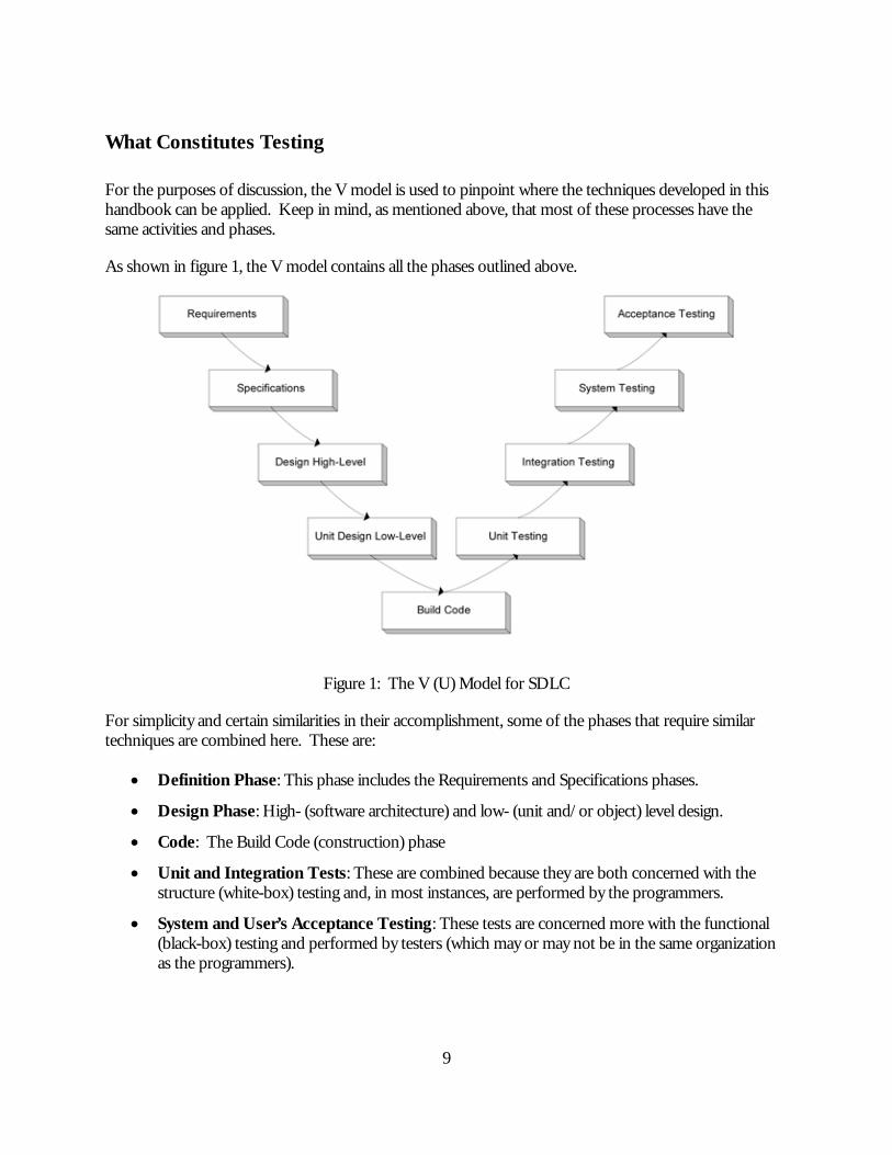
For the purposes of discussion, the V model is used to pinpoint where the techniques developed in this handbook can be applied. Keep in mind, as mentioned above, that most of these processes have the same activities and phases.
As shown in figure 1, the V model contains all the phases outlined above.
Figure 1: The V (U) Model for SDLC
For simplicity and certain similarities in their accomplishment, some of the phases that require similar techniques are combined here. These are:
• Definition Phase: This phase includes the Requirements and Specifications phases.
• Design Phase: High- (software architecture) and low- (unit and/or object) level design.
• Code: The Build Code (construction) phase
• Unit and Integration Tests: These are combined because they are both concerned with the structure (white-box) testing and, in most instances, are performed by the programmers.
• System and User’s Acceptance Testing: These tests are concerned more with the functional (black-box) testing and performed by testers (which may or may not be in the same organization as the programmers).

10
Figure 2 is a simplification of the V model and includes techniques outlined in the remainder of this handbook.
Integration and Unit Testing
Functional Requirementsand Specifications
High- and Low-LevelDesign
Construction Code
Acceptance and SystemTesting
SpecChek
Wrapping
NumericalReliability
Figure 2: Simplified V Model with Handbook Techniques
SpecChek: Used in the definition phase to organize the requirements. The specifications can be coded in XML, and SpecChek is used to produce a running version of the specifications. “What if” scenarios then can be created to consider different alternatives. This can also be used as a communication tool with users and stakeholders to clarify
ambiguities in the requirements.
After the specifications have been completed, the XML (SpecChek) version can be saved and used later on in the system and acceptance testing phases to compare SpecChek (expected) results with the system’s (actual) outputs.
Wrapping: Used to wrap pieces of code that are either critical or that communicate (their output is used by) critical code. The wrapper tests the result (output) of the wrapped code before it is passed to other parts of the system. This can be used to test structure (to verify the execution of a particular path) and function (to verify a particular function) .
Numerical Reliability: Used to verify the numerical precision and accuracy of a mathematical computation.
11
Chapter 3 Software Testing
This chapter discusses:
• Definition of software testing.
• Criteria for choosing test cases.
• Practical limitations of testing.
Definition of Software Testing
Software testing is the process of experimentally verifying that a program operates correctly. It consists of:
• Running a sample of input data through the target program.
• Checking the output against the predicted output.
Why Test?
Testing is a necessary part of establishing software correctness, even software that has been proven correct. This is because testing catches:
• Failures caused by details considered irrelevant during a correctness proof. For example, in a proof, Input/Output (I/O) operations might be ignored, because they do not affect data of interest, but if they crash, the provably correct program fails.
• Failures caused by errors that were overlooked during a correctness proof.
• Corruption of a computation by other parts of a large system.
Scope of Chapter
Only some highlights of the extensive literature on software testing are included in the handbook. Simple statistical procedures for analyzing test results are summarized in chapter 9 in Verification, Validation, and Evaluation of Expert Systems, an FHWA Handbook (5)

12
What Constitutes Testing
From a statistical standpoint, testing is an experiment, and the conclusions one can draw are governed by the theorems of statistics. In particular, for the results of testing to be statistically valid:
• A sample (in this case, the inputs for testing) must be randomly selected from the population.
• Conclusions are only valid for the population from which a sample is drawn.
For a sample to cover a population, every property of the inputs that might be expected to affect correctness should be represented sufficiently in the sample. “Sufficiently” in this context means that if a particular property causes the program to fail, inputs with that property occur frequently enough so that the failure is detectable statistically.
What to Include in the Test Sample
Wallace et al. have cataloged some of the kinds of inputs that should go into a test set.(4) These inputs must be in the test set because they have properties that might affect whether a program functions correctly.
• Boundary value analysis “detects and removes errors occurring at parameter limits or boundaries. The input domain of the program is divided into a number of input classes. The tests should cover the boundaries and extremes of the classes. The tests check that the boundaries of the input domain of the specification coincide with those in the program. The value zero, whether used directly or indirectly, should be used with special attention (e.g., division by zero, null matrix, zero table entry). Usually, boundary values of the input produce boundary values for the output. Test cases should also be designed to force the output to its extreme values. If possible, a test case, which causes output to exceed the specification boundary values, should be specified. If output is a sequence of data, special attention should be given to the first and last elements and to lists containing zero, one, and two elements.”
• “Error seeding determines whether a set of test cases is adequate by inserting (seeding) known error types into the program and executing it with the test cases. If only some of the seeded errors are found, the test case set is not adequate.”
• “Coverage analysis measures how much of the structure of a unit or system has been exercised by a given set of tests.”
• “Functional testing executes part or all of the system to validate that the user requirement is satisfied.”
• For highway-related software, this means that highway engineers should determine the range of different situations from the engineering perspective covered by the software, and ensure that all of those situations are represented in the test set. Software developers may not understand the
13
engineering significance of the software, and might not include those test cases or notice engineering anomalies in other test results.
• “Regression analysis and testing is used to reevaluate software requirements and software design issues whenever any significant code change is made.”
How to Select the Test Sample
The test sample must be random, yet contain enough of the special inputs listed above (called a stratified sample in statistics). To ensure randomness, it is important that inputs in the test set not be used during program development. If inputs are used in program development, they are not random, but become inputs used during development. There is no way to be sure that a program does not behave differently on the inputs used during development than on truly random inputs. In fact, neural nets can be over-trained to behave better on their training set than on a randomly chosen input set.
The best way to ensure that test inputs are not used during program development is to choose a test set before implementation begins, and lock that test set away from the development team.
How Many Inputs Should Be Tested
The number of inputs to test depends on the purpose of the test. To obtain a certification of correct performance to a certain confidence level, a sample that is large enough to provide that confidence level must be chosen. (See the FHWA handbook referenced above, or most elementary statistics texts for more details.) If the program is designed to compute an estimate rather than an exact value of its output, a statistically significant sample must be used.
However, for programs that compute exact values of their outputs, an argument can be made for testing a single point in a region of the input space for which:
• The program follows the same computational path for all the inputs in the region.
• The input chosen has no special properties in the program, e.g., is not a boundary point of a branch in the program, unless all points in the region have this property.
• All the inputs in the region represent similar inputs from the engineering perspective of the area of application.
If a single input from the region is correct, this was either a fluke or an event that would be replicated with further tests. For it to be a fluke, the program would have to apply some set of formulas other than the intended ones and get an identical output to the intended output for a randomly chosen point. This is a very unlikely event.

14
Limitations of Testing
Rigorous testing of large software is not possible, because the number of test cases that must be run is impractically large. For example, the PAMEX pavement maintenance expert system contains approximately 325 rules; there are millions of different possible execution paths. For this reason, testing should be supplemented with techniques such as informal proofs and/or wrapping.
15
Chapter 4 Safe Introduction of Software Using Scale Up
While software systems can contain millions of different computational paths, most are probably tested with orders of magnitude fewer test runs. This means that there may be potential failures lurking in the large population of situations that are never encountered during testing. For software that is embedded in safety critical systems, some software failures are deadly, as illustrated by the Therac-25 accidents. This page shows a method for calculating the number of expected failures when scaling up from testing to application in those situations where no failures are observed during testing.
The Problem
A safety critical program is to be run N times, where N is large, e.g., millions of times. It has been tested on a random sample of n data items from the population of production runs, where n is small, e.g., in the hundreds. No failures were observed. How many failures can be expected in a large number of runs? And how can we minimize the danger of failures?
What Is Learned from “n” Successes
The binomial distribution is the probability distribution that describes the number of failures that will be observed in N trials, if the probability of failure on a single trial is p. When at least 5 successes and at least 5 failures are observed in a large number of runs (more than 30) the normal distribution can be used to approximate the binomial distribution. However, a system from which most bugs have been removed may not fail often enough during testing to use this approximation. In these cases, Bayes’ Theorem can be used to analyze the rarely failing system.
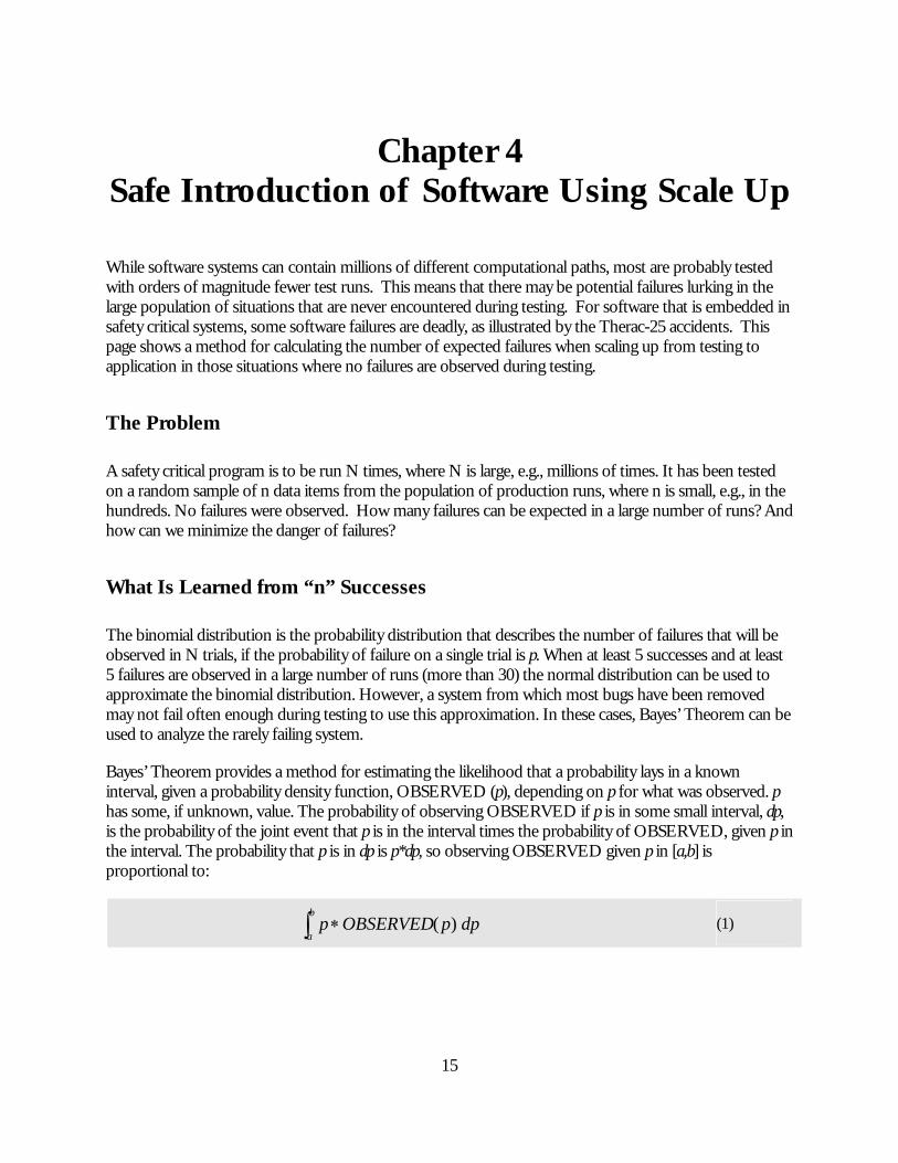
Bayes’ Theorem provides a method for estimating the likelihood that a probability lays in a known interval, given a probability density function, OBSERVED (p), depending on p for what was observed. p has some, if unknown, value. The probability of observing OBSERVED if p is in some small interval, dp, is the probability of the joint event that p is in the interval times the probability of OBSERVED, given p in the interval. The probability that p is in dp is p*dp, so observing OBSERVED given p in [a,b] is proportional to:
dppOBSERVEDpb
a)(∗∫ (1)
16
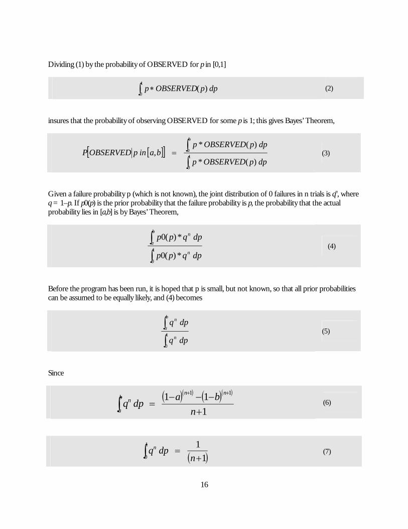
Dividing (1) by the probability of OBSERVED for p in [0,1]
dppOBSERVEDp )(1
0∗∫ (2)
insures that the probability of observing OBSERVED for some p is 1; this gives Bayes’ Theorem,
[ ][ ]∫∫= 1
0)(*
)(*,
dppOBSERVEDp
dppOBSERVEDpbainpOBSERVEDP
b
a (3)
Given a failure probability p (which is not known), the joint distribution of 0 failures in n trials is qn, where q = 1–p. If p0(p) is the prior probability that the failure probability is p, the probability that the actual probability lies in [a,b] is by Bayes’ Theorem,
∫∫
1
0*)(0
*)(0
dpqpp
dpqpp
n
b
a
n
(4)
Before the program has been run, it is hoped that p is small, but not known, so that all prior probabilities can be assumed to be equally likely, and (4) becomes
∫∫
1
0dpq
dpq
n
b
a
n
(5)
Since
( )( ) ( )( )
111 11
+−−−
=++
∫ nba
dpqnn
b
a
n (6)
( )111
0 +=∫ n
dpqn (7)
17
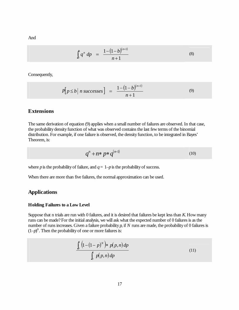
And
Consequently,
Extensions
The same derivation of equation (9) applies when a small number of failures are observed. In that case, the probability density function of what was observed contains the last few terms of the binomial distribution. For example, if one failure is observed, the density function, to be integrated in Bayes’ Theorem, is:
where p is the probability of failure, and q = 1–p is the probability of success.
When there are more than five failures, the normal approximation can be used.
Applications
Holding Failures to a Low Level
Suppose that n trials are run with 0 failures, and it is desired that failures be kept less than K. How many runs can be made? For the initial analysis, we will ask what the expected number of 0 failures is as the number of runs increases. Given a failure probability p, if N runs are made, the probability of 0 failures is (1–p)N. Then the probability of one or more failures is:
( )( )
111 1
0 +−−
=+
∫ nbdpq
nb n (8)
[ ] ( )( )
111 1
+−−
=≤+
nbsuccessesnbpP
n
(9)
( )1−∗∗+ nn qpnq (10)
( )( ) ( )
( )dpnpp
dpnppp N
∫∫ ∗−−
1
0
1
0
,
,11 (11)
18
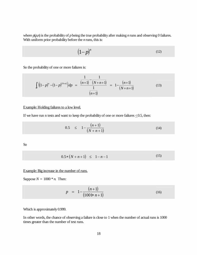
where p(p,n) is the probability of p being the true probability after making n runs and observing 0 failures. With uniform prior probability before the n runs, this is:
So the probability of one or more failures is:
Example: Holding failures to a low level.
If we have run n tests and want to keep the probability of one or more failures <0.5, then:
So
Example: Big increase in the number of runs.
Suppose N = 1000 * n. Then:
Which is approximately 0.999.
In other words, the chance of observing a failure is close to 1 when the number of actual runs is 1000 times greater than the number of test runs.
( )np−1 (12)
( ) ( )( )( ) ( ) ( )
( )
( )( )1
11
11
11
11
111
0 +++
−=
+
++−
+=−−−∫ +
nNn
n
nNndppp nNn (13)
( )( )1
115.0++
+−≤
nNn
(14)
( ) 1115.0 −−≤++∗ nnN (15)
( )( )11001
11+∗
+−=
nnp (16)

19
Conclusion
To prevent failures when a system is introduced, the deployment should be done in a succession of phases. In each phase, the number of deployments is a multiple of the deployments in the previous phase. The system is observed in the larger deployment, and this result is used as the test run in the next phase of the deployment.

21
Chapter 5 Informal Proofs
This chapter:
• Defines a framework for informal proofs about programs.
• Introduces proof techniques for informal proofs about programs.
• Contains simple examples of informal proofs.
• Discusses the application of informal proofs.
• Lists the limitations of informal proofs.
The following simple examples provide some context for the framework.
Introduction
Informal proofs are proofs similar to those of high school geometry or calculus for engineers. Informal proofs seek to retain the certainty of knowledge that comes from doing a proof while reducing the work in actually doing the proof.
Simple Examples
Here is a pair of simple illustrative proofs about the factorial function, a function that often is used to illustrate the syntax of a programming language. Although these proofs are shorter and simpler than proofs used in a real software project, they illustrate the general style and level of proof that can be achieved using the symbolic evaluation framework presented later in this chapter.
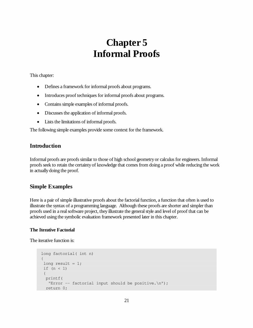
The Iterative Factorial
The iterative function is:
long factorial( int n) { long result = 1; if (n < 1) { printf( "Error -- factorial input should be positive.\n"); return 0;

22
} else if (n == 1) return 1; while (n>0) { result = result * n; n--; } return result; }
It will be proved that factorial(n) = n* ...*1 for positive integers n. (Note: factorial(n) = n*(n-1)*…*1.)
The proof is by mathematical induction. This is a common proof technique for proofs about programs. In an inductive proof, the result is proved for the simplest cases, in this case for n = 1. Then it is also proved that if the desired result holds for all inputs at a complexity of a certain amount or less, it must hold for inputs of slightly greater complexity. In this case, the second part of the proof consists of assuming the result for positive integers k or less, and proving it for k+1. In other situations, the parameter on which induction is proved might be the depth or number of nodes in a tree, or the number of execution steps in executing a program.
Proof: When n = 1, the 2nd branch of the if-else applies, and 1 is returned.
Now assume that for n = k, the function returns k*...*1, where k>1. In this case, neither branch of the if-else returns a value, and the while loop is executed. From the inductive assumption and the fact that result = 1 before the while loop, we know that when the while loop is executed with n = k, it multiplies the current value of result by k*...*1.
For n = k+1, neither branch of the if-else applies, and the while loop is executed. Because k+1>1, the loop body is executed. The first loop body execution multiplies result by k+1 and decreases n to k. After this first loop body execution, the conditions of the inductive assumption occur. Using this assumption, result is multiplied by k*...*1 during the rest of the loop execution. Altogether:
• Result begins at 1.
• The first time through the loop multiplies it by k+1.
• The rest of the loop iterations multiply it by k*...*1.
The value of result is (k+1)*k*...*1 after the loop. Because factorial returns result, the inductive part of the proof is complete, and factorial computes n*...*1.
The Recursive Factorial
The recursive function is:

23
long factorial( int n) { if (n<1) { printf( "Error -- factorial input should be positive.\n"); return 0; } else if (n == 1) return 1; else return n * factorial(n-1); }
It will be proved that factorial(n) = n* ...*1 for positive integers n.
Proof: As with the iterative case, the proof is by mathematical induction. For n = 1, the second branch of the if-else is taken, and 1 is the value of the function.
Now assume that for n = k,
factorial(k) = k*...*1
With the goal of proving
factorial(k+1) = (k+1)*k*...*1
Because k+1>1, the third branch of the if-else is taken, and (k+1)*factorial(k) is returned. By the inductive assumption, this is (k+1)*k*...*1, and the theorem is proved.
Advantages and Limitations of Informal Proofs
Informal proofs for computer programs date back at least to the 1970s. As shown by the simple examples above, proofs generally are too labor intensive for large programs. However, proofs can be useful for critical software modules because:
• The number of test cases needed to completely test a module can be very large (e.g., millions for a medium-sized expert system).
• A successful proof is a good argument that a program’s logic is correct.
• The process of constructing a proof forces the prover to study the workings of a program in detail, often exposing bugs.
Proofs by themselves are not sufficient to guarantee software correctness, because:
24
• The proof can contain errors. In particular, it is easy to see in a program what is needed for a proof but is not really in the program.
• Proofs are usually conducted on abstractions of the program that can overlook code that can cause errors, e.g., I/O statements that crash the program.
Another limitation of proofs is that they require the program source code.
Symbolic Evaluation
Most proofs about computer programs use some form of symbolic evaluation. For example, the two example proofs presented above used symbolic evaluation. This section defines the process of symbolic evaluation for use in informal proofs.
A symbolic evaluation is an abstraction of an actual computer computation. The purpose of a symbolic computation is to provide a simpler object on which to carry out a correctness proof. In addition, the symbolic computation abstracts a set of actual computations, so a single proof on a symbolic computation can be helpful in proving the correctness of an entire set of actual computations.
The following sections detail the differences and relationship between an actual and a symbolic computation.
Contents of Memory
The contents of an actual computer memory are finite precision numbers, bytes, and characters that represent the data manipulated by a computer program. They are addressed by an integer location of the first byte in memory.
The contents of a symbolic computation memory are pure mathematical objects (e.g., numbers of infinite precision, characters, strings, matrices, functions, geometric figures, and any other objects used in the algorithm being considered). Each of these is the value of some variable, either an explicitly stated variable name from the symbolic program, or a description of what the data item is. Symbolic objects are addressed by asking for the value of this variable.
In addition, objects in symbolic memory need not be values, but can contain variables. For example, symbolic objects can be mathematical expressions that compute the value of an object—instead of the finite precision number that would represent speed in a real computer memory, a symbolic memory would contain the value of a speed variable. This might be an infinite precision number, another variable representing speed, or an expression (such as distance/time).

25
Currently True Statements
In a symbolic computation, assumptions in the form of equations, inequalities, and logical statements often are made about the variables in the symbolic memory. These assumptions express what is known about:
• The real-world objects the software concerns, e.g., ranges for design parameters such as lane width.
• Mathematical properties of input parameters and other variables, e.g., that the input to the factorial is a non-negative integer.
During the course of a symbolic computation, the set of currently true statements:
• Is changed by actions of the symbolically executing computer program.
• May be supplemented by mathematically proved or, in some applications, empirical observations.
Two sets of currently true statements are considered equivalent if each statement in one set can be proved using statements in the other set.
Symbolic Programs
A symbolic program is a pseudocode-like abstraction of an actual program. A symbolic programming language contains a known finite set of programming operations such as assignment; blocks; if-then-else branching; loops such as while, do, and for; and perhaps try-catch exception handling. Each of these operations is defined by a transition rule that changes the contents of symbolic memory, the current point of execution of the symbolic program, and the set of currently true statements; examples are provided below after some further definitions.
The syntax of a symbolic program is not specified in detail, but must satisfy the requirement that a symbolic program can be parsed unambiguously into a semantic tree structure in which:
• Each node is a symbolic programming operation.
• The subnodes and their relation to the parent are identified, e.g., that the test and loop body of a while statement can be identified.
Point of Current Execution
At any time, the point of current execution of a symbolic program is known. The point of current execution specifies the next statement in the program, if any, to be executed, or that the program has terminated. At the start of program execution, the point of current execution is before the first statement of the program.

26
Threads
Together, the contents of symbolic memory, the set of currently true statements, and the point of current execution define the state of a single thread of a symbolic computation. As noted below, a symbolic computation sometimes splits into multiple threads. For a theorem to be proved for a symbolic computation, it must be proved for all the threads that split off successor states to the start state of the symbolic program.
Transition Rules
Following are the transition rules for the symbolic form of some common programming operations. They describe how to change the symbolic memory, currently true statements, and point of current operation after executing the different types of statement in a symbolic programming language, which models the typical procedural programming language.
The changes these statements make is what would be expected based on experience with these programming languages; our experience with programming languages allows us to describe the effects of a single statement on a symbolic computation representing a set of actual computations. By reasoning about the cumulative effect of these statements as they are executed, one after another, for the entire program, something can be proved about the effect of running an entire program that belongs to the set represented by the symbolic computation.
Source of the Transition Rules
The transition rules presented below derive from the definitions of the basic statement types of standard procedural programming languages, as a result of asking, “Given how a statement changes an actual computer running a single program starting with a single set of inputs, how does that same statement affect a symbolic computer running multiple instances of a program each of which starts with different inputs?”
Assignment
When a statement
x = y
is executed,
• The variable x is added to symbolic memory if it was not there.
• The variable y replaces any previous value of x in symbolic memory.
• The equality x = y is added to the currently known statements and replaces any previous statements of the form x = [whatever].

27
• Any statement in the currently true statement that depends on the old x = [whatever] is deleted.
• The point of current execution moves to the statement after the assignment, or to the end of the program if there is no such statement.
In the assignment statement, x must be a variable and y a mathematical expression for the type of object that is the values of x.
While stating all this about assignment makes it appear complicated, the above statements just express our intuition about what assignment in a procedural language means.
Blocks
A block is a sequence of statements enclosed in syntactic markers (e.g., {and} in C and Java™. This converts a sequence of statements into a single statement in the programming language.
When a block is executed, each of the statements in the block is executed in the sequence they appear in the block. As each statement is executed, the changes it makes in the symbolic memory and currently known statements are carried out. After the last statement of the block is executed, the point of current execution moves to the statement after the block or to the end of the program.
If-Else
An if-else statement consists of a Boolean-valued test, a statement executed when the test evaluates to true, and an optional statement executed when the test evaluates to false.
In symbolically evaluating an if-else, an attempt is made to prove the test from the currently true statements. If this attempt succeeds, the then statement (the statement intended for execution if the test is true) is executed symbolically.
If the test cannot be proved, but can be shown to contradict the currently true statements, the else statement (the statement intended for execution if the test is false) is executed symbolically, if an else statement is present.
If the test is sometimes true and sometimes false given the currently true statements, or if the test can neither be proved nor disproved from the currently true statements, the symbolic computation is split into two symbolic computations. In one, the test is added to the currently true statements. In the other, the negation of the test is added. For a statement to be proved for the original symbolic computation, it must be proved in each of these new symbolic computations. This situation is similar to that in pure mathematics, when a theorem is proved by breaking it into a set of special cases, each of which is proved in turn.
After determining which branch or branches of the if-else statement must be executed, those branches are symbolically executed, with the test added to the currently true statements when executing the then

28
statement and the negation of the test added when executing the else statement, if there is an else statement.
After executing the then and/or else statements, or after executing none if there is no else statement and the test is symbolically false, the point of current execution is set to the statement after the if-else, or to the end of the program, in the one or possibly two symbolic computations that now exist.
After executing the if-else statement, the currently true statements are as follows:
• In the computation where the test was symbolically true:
o The test is added to the incoming currently true statements.
o The currently true statements are modified using the symbolic evaluation rules that apply to the then statement.
• In the computation where the test was symbolically false:
o The negation of the test is added to the incoming currently true statements.
o If an else statement is present, the currently true statements are then modified using the symbolic evaluation rules that apply to the else statement.
While
A while statement contains a test and a loop body. In symbolically executing the while statement, it must be proved that after a finite number of symbolic executions of the loop body, the test can be proved to be false. (If the test can be proved to be false with no loop repetitions, this condition is satisfied.) If the test cannot be proved to eventually fail, the symbolic computation ends in an error state.
If the while loop is proved to terminate after symbolically executing a while statement, the point of execution is the statement after the while statement or the end of the program.
If the test is not provably false, the contents of symbolic memory are changed in accordance with the symbolic evaluation rules for enough loop repetitions to make the test false. If the test is provably false, the contents of symbolic memory are unchanged.
The currently true statements after a while loop are computed by:
• Starting with the currently true statements that have accumulated up to the while loop.
• Changing the state of the symbolic computation (if the test is not provably false), including the currently true statements, as the result of enough loop executions to make the test false.
• Adding the negation of the test to the currently true statements.
For and do loops are executed in a similar way.

29
Function Calls
When a function is called, variables are added to symbolic memory representing function parameters. For pass-by value, the variable value is copied. For pass-by reference, the new variable name is added as a name to reference an existing object in memory. Variables declared within the function body are added when values are assigned to those variables.
After adding parameters to memory, statements in the function body are executed using the rules of symbolic evaluation.
When the function code is completed, t he variables representing function parameters or declared in the function body are removed from symbolic memory. Statements involving these variables are removed from the currently true statements.
After a function call, the point of current execution is just after the function call or at the end of the program.
Object Creation
In object-oriented languages, if an object is created, a variable name and the new object as value are added to symbolic memory. If a variable name for the object appears in the program, it is used; otherwise a name that unambiguously identifies the new object is created for it. The point of execution moves to after the new (object-creation) operation. The currently true statements are unchanged.
Object Destruction
When an object is destroyed because the program moves outside the scope of the object or because of an explicit-free operation, the object is removed from symbolic memory. Statements involving the object are removed from the currently true statements. Execution moves to after the destroy operation.
Read
As with assign, a read operation adds a variable name and corresponding value to symbolic memory. The currently true statements are updated to include any assumptions made about input values. The point of execution moves to after the read statement.
Write
To model the write operation, an abstract output destination is assumed. It is assumed that the value of objects in symbolic memory, including symbolic values (those containing variables), can be written to this destination. It is also assumed that the capacity of the symbolic destination is infinite, and that the values can be read by the outside world in the order in which the values were written.
A write statement adds a constant or a value in symbolic memory to the symbolic output. The currently true statements are generally unchanged, although the truth of statements of the form “x has been

30
written” may change. The point of current execution moves to after the write statement or to the end of the program.
Try-Catch
In a symbolic try-catch computation, the recommended procedure is to split the symbolic computation into one try and one catch thread. The first represents normal execution and the second represents the raising of an exception. Both threads must be considered because it cannot be proved that an exception will not occur. This is because every computation uses a wealth of underlying software and depends on physical devices.
However, in some cases, an argument that an exception will never occur may become part of the informal proof.
A third option may be to restrict what is being proved to cases where an exception does not occur. In this case, this assumption should be stated clearly.
The rules for blocks are applied to evaluate the two threads of a try-catch computation, using the try block for one thread and the catch block for the other. As with if-else statements, a desired theorem must be proved for both threads, unless it is proved that an exception cannot occur (doubtful), or exceptions are excluded explicitly in the theorem to be proved.
Using a Proof in V&V
A proof shows that the logic of the algorithm implemented by a program is correct. However, to show that a program actually is correct, one must demonstrate that the program implementing the algorithm and the physical computer on which it runs actually carry out the algorithm with enough accuracy for the application.
The following items are among those that should be checked to ensure that an algorithm proved to be correct works when implemented:
• The program accurately implements the algorithm.
• Numbers are within the range of computer arithmetic. The factorial functions only have this property for the small integer values.
• Numerical calculations are free from serious numerical errors. A technique for doing this is presented in chapter 5.
• The computer has enough memory to carry out the computation.
• The computation finishes in a reasonable time.
• The program does not crash because of operating system, file, or the Graphical User Interface (GUI) errors.

31
Chapter 6 Wrapping
This chapter:
• Explains how verification code within a program can make the program self-testing.
• Documents how to use executable specifications to implement wrapping for highway software.
• Discusses a sample highway application.
• Outlines what is gained from wrapping.
• Lists the limitations of wrapping.
Introduction
A wrapping for a piece of software is additional information that the software can use to answer questions about itself. The concept of wrapping was originally developed in National Aeronautics and Space Administration (NASA) sponsored work on large systems.(6) An intended application of wrapping was to allow software to describe its function to make it easier to call the right function in a large software project.
Wrapping also appears in Java in the form of the “instanceof” relation and the reflect package. These facilities allow objects to report on their contents and class membership.
Applied to software correctness, wrapping is a technique that uses a modified version of a piece of software to compute its own correctness. To wrap a program P used in system S with a requirement R on P:
• R is translated (using the techniques for translating formulas) into an equivalent representation R' in the programming language of P.
• R' is inserted at the end of P, right before P returns its value(s). This insertion is done in such a way that the calling context of P can examine the result of R. The modified version of P will be called P'.
• S is modified to:
o Test the value of R'.
o Discard the values from P' if R' is FALSE.
32
Wrapping has several different V&V applications:
• Wrapping a software module with a logical formula specification.
• Wrapping a software module with necessary but not sufficient conditions for correctness that the output must satisfy. This is useful when sufficient conditions for correctness are not available, e.g., with software that predicts values that have not yet been observed.
• Wrapping inputs to all programs to ensure that the inputs are in the domain for which the program is intended.
Several examples follow.(3)
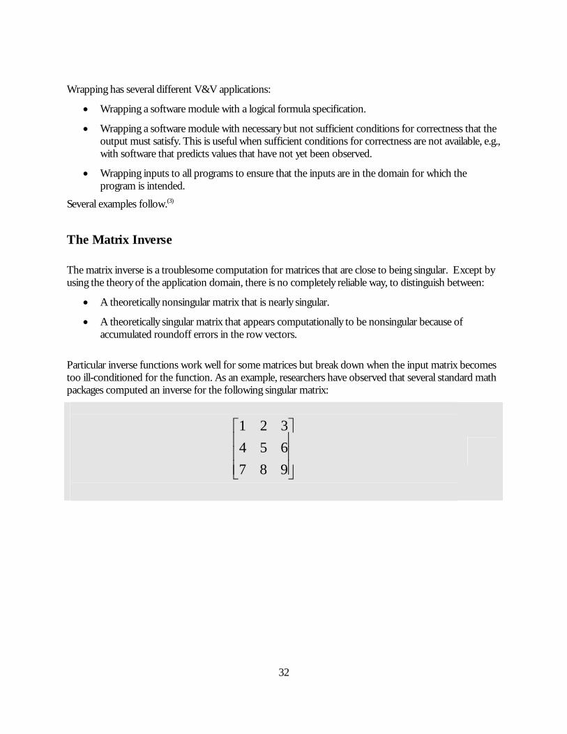
The Matrix Inverse
The matrix inverse is a troublesome computation for matrices that are close to being singular. Except by using the theory of the application domain, there is no completely reliable way, to distinguish between:
• A theoretically nonsingular matrix that is nearly singular.
• A theoretically singular matrix that appears computationally to be nonsingular because of accumulated roundoff errors in the row vectors.
Particular inverse functions work well for some matrices but break down when the input matrix becomes too ill-conditioned for the function. As an example, researchers have observed that several standard math packages computed an inverse for the following singular matrix:
⎥⎥⎥
⎦
⎤
⎢⎢⎢
⎣
⎡
987654321

33
Problems with the matrix inverse can be due either to numerical roundoff errors or to an underlying problem in the computer code. One of the math packages that has a problem with this matrix is Numerical Recipes in C.(7) The code segment that seems to cause the problem is:
float big; big=0.0; for(j=1;j<=n;j++) {if((temp=fabs(a[i-1][j-1])) > big) big=temp; } if (big==0.0) Error("singular matrix",1);
This is the only point in the matrix inverse function that tries to detect singular matrices. It apparently fails because it is possible for both >0 and == 0 to fail for very small positive numbers (something that cannot happen in abstract mathematics of the real numbers). For reasons like this, it is considered good practice in writing numerical software to avoid strict equality tests with 0 and instead to write a test like:
if (big< EPSILON) Where EPSILON is some number chosen to catch very small numbers that are more likely due to roundoff errors than legitimate results of numerical computations.
However, no choice of EPSILON truly can separate actual and false inverses all the time. So instead:
• EPSILON is passed in as a parameter.
• The definition of the inverse, i.e., A*inv(A) = inv(A)*A = I is used to test that the computed inverse is actually an inverse to within EPSILON.
int wrapped_inverse( double * in, double ** out, int dim) { double * possible_inverse; double * possible_identity; double * identity; inverse( in, &possible_inverse, dim); multiply( in, possible_inverse, &possible_identity, dim); identity( &identity, dim); if (distance( identity, possible_identity) > EPSILON ) return(0); multiply( possible_inverse, in, &possible_identity, dim); if (distance( identity, possible_identity) > EPSILON ) return(0); else return(1); }
34
Where:
• Matrices are represented by pointers to the first (0 index) double (real number).
• Inverse, multiply, identity, and distance have the purposes suggested by their names.
• Outputs are represented by pointers to arrays that hold the computed information (pointers to pointers to doubles in C).
Note that wrapped_inverse:
• Sets a pointer (out) to point to the possible inverse.
• Returns a truth value (as an integer) that indicates whether the identity computed by trying the possible inverse is close to the true inverse.
As a result, the caller of wrapped_inverse always knows whether the computed inverse really works as an inverse.
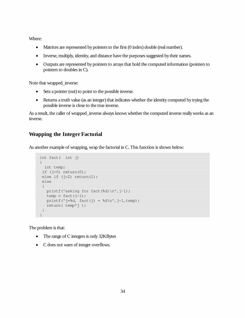
Wrapping the Integer Factorial
As another example of wrapping, wrap the factorial in C. This function is shown below:
int fact( int j) { int temp; if (j<0) return(0); else if (j<2) return(1); else { printf("asking for fact(%d)\n",j-1); temp = fact(j-1); printf("j=%d, fact(j) = %d\n",j-1,temp); return( temp*j ); } }
The problem is that:
• The range of C integers is only 32KBytes
• C does not warn of integer overflows.
35
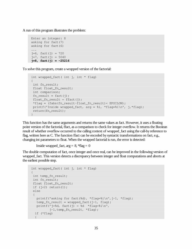
A run of this program illustrates the problem:
Enter an integer: 8 asking for fact(7) asking for fact(6) ... j=6, fact(j) = 720 j=7, fact(j) = 5040 j=8, fact(j) = -25216
To solve this program, create a wrapped version of the factorial:
int wrapped_fact( int j, int * flag) { int fn_result; float float_fn_result; int comparison; fn_result = fact(j); float_fn_result = ffact(j); *flag = (fabs(fn_result-float_fn_result)< EPSILON); printf("Inside wrapped_fact, arg = %i, *flag=%i\n", j,*flag); return(fn_result); }
This function has the same arguments and returns the same values as fact. However, it uses a floating point version of the factorial, ffact, as a comparison to check for integer overflow. It returns the Boolean result of whether overflow occurred to the calling context of wrapped_fact using the call-by reference to flag, written here as C. The function ffact can be encoded by syntactic transformations on fact, e.g., changing int parameters to float. When the wrapped factorial is run, the error is detected:
Inside wrapped_fact, arg = 8, *flag = 0
The double computation of fact, once integer and once real, can be improved in the following version of wrapped_fact. This version detects a discrepancy between integer and float computations and aborts at the earliest possible step.
int wrapped_fact( int j, int * flag) { int temp_fn_result; int fn_result; float float_fn_result; if (j<2) return(1); else { printf("asking for fact(%d), *flag=%i\n",j-1, *flag); temp_fn_result = wrapped_fact(j-1, flag); printf("j=%d, fact(j) = %d *flag=%i\n", j-1,temp_fn_result, *flag); if (*flag) {
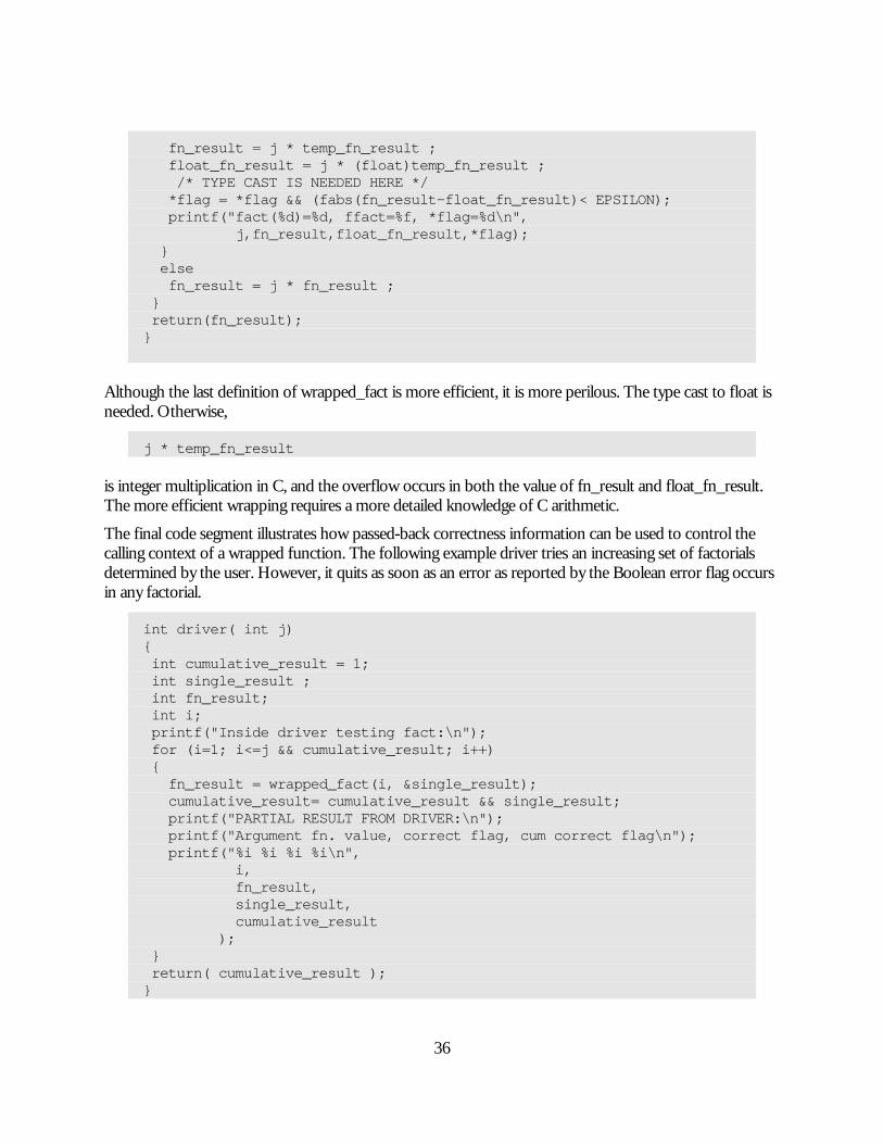
36
fn_result = j * temp_fn_result ; float_fn_result = j * (float)temp_fn_result ; /* TYPE CAST IS NEEDED HERE */ *flag = *flag && (fabs(fn_result-float_fn_result)< EPSILON); printf("fact(%d)=%d, ffact=%f, *flag=%d\n", j,fn_result,float_fn_result,*flag); } else fn_result = j * fn_result ; } return(fn_result); }
Although the last definition of wrapped_fact is more efficient, it is more perilous. The type cast to float is needed. Otherwise,
j * temp_fn_result is integer multiplication in C, and the overflow occurs in both the value of fn_result and float_fn_result. The more efficient wrapping requires a more detailed knowledge of C arithmetic.
The final code segment illustrates how passed-back correctness information can be used to control the calling context of a wrapped function. The following example driver tries an increasing set of factorials determined by the user. However, it quits as soon as an error as reported by the Boolean error flag occurs in any factorial.
int driver( int j) { int cumulative_result = 1; int single_result ; int fn_result; int i; printf("Inside driver testing fact:\n"); for (i=1; i<=j && cumulative_result; i++) { fn_result = wrapped_fact(i, &single_result); cumulative_result= cumulative_result && single_result; printf("PARTIAL RESULT FROM DRIVER:\n"); printf("Argument fn. value, correct flag, cum correct flag\n"); printf("%i %i %i %i\n", i, fn_result, single_result, cumulative_result ); } return( cumulative_result ); }

37
In turn, this function returns a success value that can control its calling context:
int main() { int result; /* result of driver */ int j; /* scope is main */ printf("Enter an positive integer.\n"); printf(">>"); scanf("%d", &j); if (j>=1) { result = driver(j); if (result) printf("*****RESULT OF %i FACTORIALS IS TRUE", j); else printf("*****RESULT OF %i FACTORIALS IS FALSE", j); } return(0); }
The complete output of the above source code is listed in appendix A.
Limitations of Wrapping
Wrapping, at least as shown in the examples, where wrapping code is placed directly in the source code, has the following limitations:
• The source code is necessary to wrap.
• An error in the wrapping code may lead to a false positive, in which an error is flagged but none exists in the wrapped computation.
• An underlying problem, such as an error in a procedure called both by the main computation and its wrapping, can cause a false negative: An error exists but is not caught by the wrapping.
• Large, complex specifications, which are typical for engineering applications, are difficult to code as wrappings.
Wrapping with Executable Specifications
To overcome the wrapping limitations caused by writing wrapping code directly in the source, write the specifications in a more declarative but computer-executable form, as is done in expert systems. This:

38
• Reduces coding errors in the wrapping code.
• Provides a practical way to use large complex engineering specifications in a wrapping.
Then call the wrapping code external to the wrapped program, and apply the wrapping to files of inputs and outputs of the target program. This allows wrapping to be used even if source code is not available. The particular form for the specification knowledge base that will be used is a set of decision trees. This knowledge representation and the software for using it are discussed below.
Knowledge Representation of Specifications
Decision trees are useful in formalizing specifications, because:
• Decision trees break a problem into successively smaller subproblems. This allows the domain expert to use a divide-and-conquer strategy in writing and checking specifications.
• Decision trees mirror many informal specifications, e.g., large parts of the specifications for the Interactive Highway Safety Design Model (IHSDM) policy module.
• Tools can be written to automatically check the consistency and completeness of the decision tree.
• A decision tree interpreter can apply a decision tree of specifications as a wrapping to enforce the specifications at runtime.
When decision trees are used to check the results of a computer program, the decision tree returns a Boolean value: true if the decision tree is satisfied, and false if not. The inputs to and outputs from the program are used as values of variables referred to in the decision tree. The rules for computing the Boolean value of the decision tree are listed in the section below.
Decision Tree Nodes for Representing Specifications
• Or: Is satisfied if at least one of its subnodes is satisfied. The subnodes of an “or” node can be “or,” “and,” “ifthenelse,” “test,” or “action” nodes.
• And: Is satisfied if all its subnodes are satisfied. The subnodes of an “and” node can be “or,” “and,” “ifthenelse,” “test,” or “action nodes”.
• IfThenElse: Is satisfied if one of its subnodes is satisfied. The subnodes of an “ifthenelse” node must be an “ifthen” or an “else” node. The “else” node must appear last, and the nodes must be tried in order.
• IfThen: Is satisfied if both its “if” and “then” subnodes are satisfied; otherwise the node fails. The “ifthen” node has only one “if” subnode and only one “then” subnode.
• Else: Has a single subnode of any type, and is satisfied when its subnode is satisfied.

39
• If: Is logically like an “and” node. It is satisfied if all its subnodes are satisfied. The “if” node is not necessary logically, but is convenient in formalizing informal specifications. The subnodes of an “if” node can be “or”, “and”, “ifthenelse”, or “test” nodes.
• Then: Is logically like an “and” node. It is satisfied if all its subnodes are satisfied. The “then” is not necessary logically, but is convenient in formalizing informal specifications. The subnodes of a “then” node can be “or”, “and”, “ifthenelse”, “test”, or “action” nodes.
• Test: Is satisfied if the Boolean expression enclosed within text brackets is true. “Test” nodes are C-like Boolean expressions containing constants and values of decision tree variables. “Test” nodes have no subnodes.
• Action: Is satisfied if the action presented in the node is executed successfully. Actions include C-like assignment statements that set decision tree variables or write output to a file. Action nodes have no decision tree subnodes.
An example decision tree for part of the IHSDM design speed module appears later in this chapter.
Deriving Useful Specifications
Good specifications are important in creating reliable software; but specifications are notoriously incomplete and vague. SpecChek helps create more complete, precise specifications because it lets users incrementally develop and test specifications. Use SpecChek with the following plan to create precise, complete, and enforceable specifications for software projects:
1. Collect items to include in the specifications: The specifications may be organized into a single document (e.g., the Highway Capacity Manual), but if not, collect individual specification items from experts, existing projects, and specification documents.
2. Conduct a safety analysis of the project using the software to determine how software errors might compromise safety (see Safeware, System Safety and Computers for details).(2) Then add specific items to the software specifications to prevent these errors.
3. Organize the specifications into a version 0 decision tree. Do not worry at this point about converting the tree into SpecChek’s XML notation.
4. Encode the version 0 tree into XML. See syntax.htm linked from the SpecChek homepage for information about how to do this.(8)
5. Gather input and output parameter data from successful previous projects, as well as good and bad designs.
6. Run the data from these real and imaginary projects through SpecChek and examine the results.
7. When SpecChek approves a bad design or fails a good one, use the SpecChek report to find possible errors in your evolving decision tree of specifications. Fix any errors, and if the decision tree is changed, repeat steps 5 and 6.

40
Translating Informal Specifications into Decision Trees
Translate informal specifications by applying the following set of transformational rules to a partially translated specification, until the informal specification is completely translated into a decision tree. To represent the partially finished translation, the above decision tree specification will be modified to allow each node to have a special text subnode.
The contents of the text node will be the part of the informal specification that is relevant to a decision tree node, and have not yet been translated into explicit decision tree nodes. A node with a text subnode will be considered to be satisfied if the satisfaction properties stated above are satisfied and the contents of the text node are satisfied.
With these conventions, the starting point for translating an informal specification is the decision tree:
<and> <text> [put the entire informal specification here] </text> <and>
Partial Translation Transformations
The following transformations of decision tree nodes with text carry out the translation of informal specifications into a decision tree without text nodes step by step. The set of rules below is a first attempt, and additional rules are expected to be found from translating informal specifications.
Different Topics
A decision tree from an informal specification addressing different topics is the and of the decision trees of those topics. Given a node of the form,
<and> <text> topic1, ... topicN </text> </and>
transform to
<and> <and><text> topic1</text></and> ... <and><text> topicN</text></and> </and>
Sequential Branching
Given a node of the form,

41
<and> <text> if P1 then text1 if P2 then text2 ... otherwise textN </text> </and>
transform to
<ifthenelse> <ifthen> <if> <text> P1 </text> </if> <then> <text> text1 </text> </then> </ifthen> <ifthen> <if> <text> P2 </text> </if> <then> <text> text2 </text> </then> </ifthen> .... <else> <text> textN </text> </else> </ifthenelse>
And Translation
If a text presents a set of requirements R1,..,RN that must all be satisfied, transform
<and><text>text(R1...RN) </text> </and> into <and> <and><text> text(R1) </text> </and> ... <and><text> text(RN) </text> </and> </and>
Or Translation
If a text presents a set of requirements R1,..,RN that is satisfied if any are satisfied, transform
<and><text>text(R1...RN) </text> </and>

42
into
<or> <and><text> text(R1) </text> </and> ... <and><text> text(RN) </text> </and> </or>
Atomic Formula Translation
If text can be translated into an atomic formula A, transform
<then><text>text </text> </then> into
<then><action>A </action> </then>
A similar transformation holds for tests.
Empty Text Node Deletion
Transform
<node> subnode1,...,subnodeN <text> </text> </node>
into
<node> subnode1,...,subnodeN </node>
Logical Equivalence Simplification
A tree can be transformed if its logical value is never changed. An example is double and elimination. Transform
<and><and> [whatever] </and> </and> into <and> [whatever] </and>
SpecChek
SpecChek is a computer program that interprets decision trees of the type described above, developed as part of this handbook project. When a specification is written as a decision tree, SpecChek can be used to

43
determine whether a program meets its specifications.
An executable version of SpecChek and complete user documentation is available on the SpecChek homepage.(8)
How SpecChek Is Used
The following diagram shows how SpecChek is used in checking software against its specifications.
Legend: DT = “decision tree”
Figure 3: Model of SpecChek Method
Preparations for Checking Software
Before running SpecChek:
• Develop specifications for the planned software.
• Translate the specifications into a SpecChek decision tree.
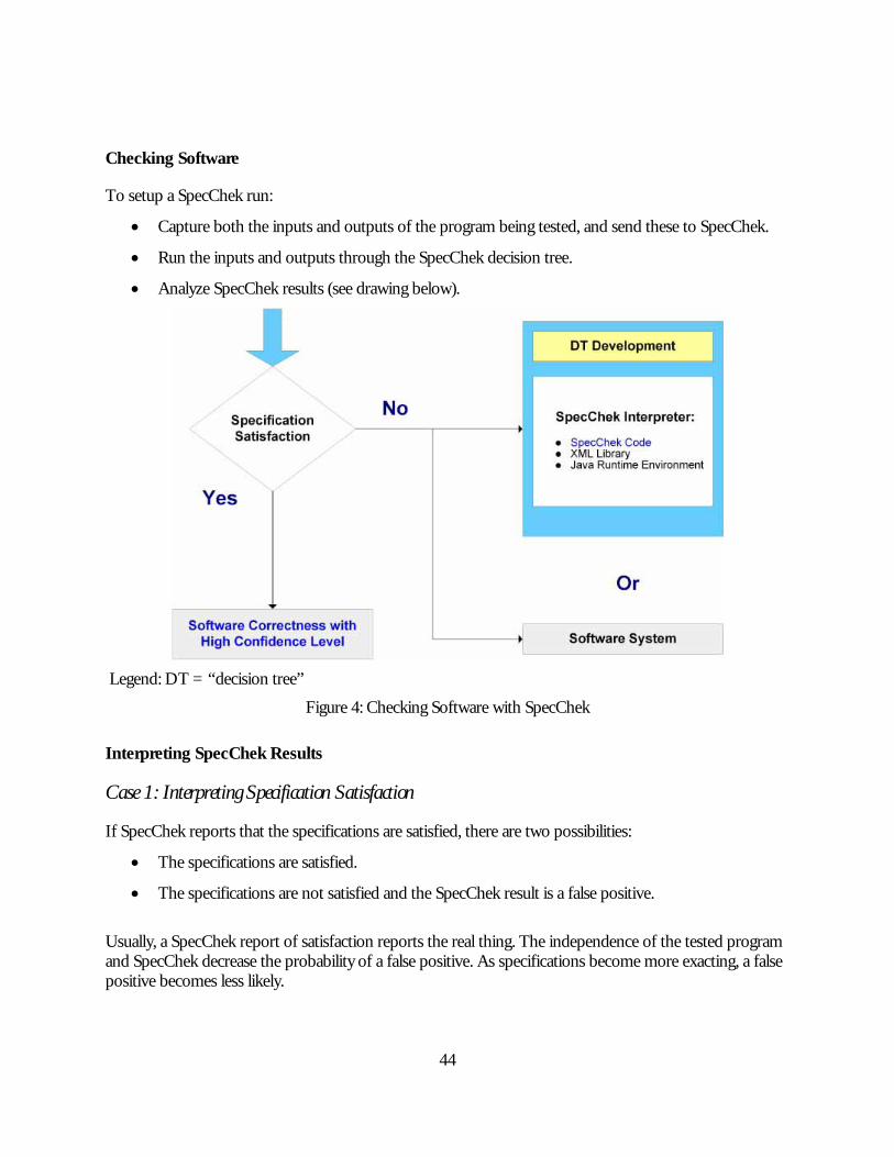
44
Checking Software
To setup a SpecChek run:
• Capture both the inputs and outputs of the program being tested, and send these to SpecChek.
• Run the inputs and outputs through the SpecChek decision tree.
• Analyze SpecChek results (see drawing below).
Legend: DT = “decision tree”
Figure 4: Checking Software with SpecChek
Interpreting SpecChek Results
Case 1: Interpreting Specification Satisfaction
If SpecChek reports that the specifications are satisfied, there are two possibilities:
• The specifications are satisfied.
• The specifications are not satisfied and the SpecChek result is a false positive.
Usually, a SpecChek report of satisfaction reports the real thing. The independence of the tested program and SpecChek decrease the probability of a false positive. As specifications become more exacting, a false positive becomes less likely.

45
Case 2: Interpreting Specification Failure
If SpecChek reports that the specifications fail, there may be an error in:
• The program being tested.
• The decision tree encoding the specifications.
• The SpecChek software.
• The supporting infrastructure (e.g., the hardware, operating system, Java libraries).
Finding the Cause of Failure
To find the cause of specification failure with such a diverse set of possible errors, use SpecChek’s reasoning report to see why SpecChek thinks the specifications fail. The error can be located by checking the logic in this report.
As illustrated in the example below, the error is usually in the program being tested. When developing or using a new decision tree, the error is sometimes in the decision tree or in the specifications put into the tree.
Although it has not been reported yet, it is possible that the error is in SpecChek or in the infrastructure for SpecChek. However, while most programs hide their errors inside the computer, SpecChek provides all the information users need to either verify SpecChek’s correctness or pinpoint its error.
The Importance of the Reasoning Report
The reasoning report of why a program passed or failed the specifications is a key to checking the performance of deployed software. Because of the low probability of false positives, reports of specification satisfaction need not be checked thoroughly. For reports of specification failure, a report of the reasoning behind failure provides a practical way for engineers or other domain experts to determine whether and why the target program actually failed. Because the reasoning report allows the identification of false negatives due to errors in SpecChek, having a readable reasoning report makes it possible to use SpecChek even though the application may contain bugs. This is important, because it is not possible with today's technology to guarantee that any piece of software as large as SpecChek is free of bugs, or that a particular run is free of errors caused by the underlying computer system. (Of course, if there are too many false positives, SpecChek is not useful. However, experience to date has not revealed any false positives from the current version.)
More about the Reasoning Report
This section discusses how to interpret SpecChek’s reasoning report in greater detail.
Interpreting a Report of Satisfaction
If SpecChek reports that the decision tree of specifications was satisfied, there are two possibilities:

46
• The report of satisfaction is a false positive, i.e., there is an undetected failure of the supplied input and output data to meet the specifications.
• The program being tested actually satisfied the specifications.
Satisfying engineering decision trees usually involves satisfying equations up to a small error tolerance and satisfying numerical inequalities that specify acceptable ranges for output variables. To estimate accurately the probability that such specifications were satisfied while both SpecChek and the target program contained errors generally requires problem-specific reasoning. However, the general comments below show that this probability is usually very small for engineering applications.
Most engineering specifications contain formulas that are applied to inputs. The chance that two erroneous calculating agents (SpecChek and the target program) would randomly produce equal results (within tolerance) out of all the possible real number answers is very small, provided that the computations resemble Bernoulli trials (the SpecChek and target program calculate their results independently).
Complete independence of the SpecChek and target program calculations generally are not achieved. For example, both may be run on the same computer, so errors in the arithmetic chip could produce outcancelling errors in each computation.
However, the following implementation features make SpecChek’s calculations significantly independent of those in the target program:
• SpecChek does not use any target program subroutines; it uses software only in the Java runtime environment, XML libraries, and the SpecChek decision tree interpreter (a compiled Java program).
• If the target program is not in Java, SpecChek and the target program are independent at the compiler and runtime library level. If the target program is in Java, there is a reasonable chance that the two programs are compiled on different versions of the Java environment.
In addition, SpecChek contains various features that were designed to minimize errors to decrease the probability of a false positive. These are discussed in more detail below.
Because the probability of a false positive is small, a report of specification satisfaction reasonably can be interpreted as actual specification satisfaction.
Other Sources of False Positives
The above discussion focused on false positives that are due to outcancelling errors in the target program in SpecChek. However, there is also the possibility that a specification failure was not found because the XML decision tree did not correctly encode the underlying engineering specification.
There is no guaranteed way to eliminate this source of error. However, it can be minimized by carefully writing and reviewing the specifications. Because the XML specifications are relatively brief and readable by engineers, this checking and review is feasible. If carried out by multiple independent reviewers, it is likely to catch most errors. The reliability of a decision tree also is increased by basing the decision tree on established engineering specifications. These specifications generally have been subjected to intensive

47
reviews, so that errors in the decision tree probably occur from translating the natural-language specifications into XML rather than from errors in the specifications themselves.
For a discussion of estimating errors in knowledge bases, see Verification, Validation, and Evaluation of Expert Systems, an FHWA Handbook.(5)
Interpreting a Report of Failure
If SpecChek reports that the decision tree of specifications was not satisfied, there are two possibilities:
• The report of satisfaction is a false negative (there is actually nothing wrong with the program being tested).
• The program being tested actually fails the specifications.
As discussed below, care has been taken to reduce the probability of an error in SpecChek. However, it is assumed that SpecChek, like almost all software, contains some bugs. When specifications are not satisfied, it must be determined whether the error is in SpecChek or in the program being tested.
The way to make this determination is to manually check the reasoning in the SpecChek report. This report describes why SpecChek thinks the decision tree is not satisfied; it is usually one page or less—small enough to be reviewed manually.
If the reasoning in the SpecChek report is sound, the error is in the target program. If the reasoning in the SpecChek report is unsound, the error is in SpecChek.
However, sometimes the specifications were not satisfied because the target program was correct and there was an error in the specification decision tree. Examining the chain of reasoning in the SpecChek report should help locate errors in the decision tree.
SpecChek’s Own Reliability
SpecChek, like almost all software, likely contains bugs. This section discusses:
• How SpecChek bugs affect the results obtained from SpecChek.
• How the design of SpecChek reduces the likelihood of bugs.
How SpecChek Bugs Affect Users
It does not matter for a particular specification satisfaction report whether SpecChek contains bugs in general; what matters is whether one of those bugs has made that particular report incorrect. This can be determined by manually checking the SpecChek report for the reasoning that led to its conclusion about specification satisfaction. If the reasoning in the SpecChek report is sound based on the decision tree of specifications, the conclusion is valid, even if the SpecChek software contained bugs, and even if some of these bugs were activated in the SpecChek computation. Because SpecChek reports its reasoning, the significance of SpecChek bugs is reduced, and any such bugs are as easy to find as possible.

48
How the Design of SpecChek Reduces the Likelihood of Bugs
• SpecChek uses a compiler and software libraries that are extensively used in other applications, namely:
o The Sun Microsystems Java 2™ compiler and runtime libraries: These are used in the very large number of Java application programs. SpecChek uses a relatively modest subset of Java and avoids such potentially error-prone areas as the control of threads (concurrent processes).
o Standard XML libraries (currently the Sun Microsystems XML implementation): XML increasingly is used as a standard for sending database information over the Internet, creating a vast application pool to detect errors in the underlying libraries.
• The SpecChek decision tree interpreter is a relatively small, well-organized program that can be read and manually checked by SpecChek subscribers who wish to verify the correctness of the code themselves
• The software developer is currently carrying out an informal correctness proof of the decision tree interpreter.
Using SpecChek in the Software Life Cycle
During the software life cycle, SpecChek can be used to promote software reliability:
• During specification development, to test specifications.
• During design, as a rapid prototyping tool (SpecChek has extensions not used in specification checking that turn the software into an expert system shell).
• As a testing tool.
• During deployment and maintenance to detect software failures.
Advantages of SpecChek for Wrapping
• SpecChek puts the professional in control of checking computed results.
• SpecChek provides an independent check of computed results, because:
o It uses its own software, not subroutines of the program being tested, to perform the necessary computations for checking output of the target program
o The professional can write and self-check the specifications being applied to the target program.

49
• SpecChek can be called from within a target program to provide real-time checking of all computed results, or SpecChek can be used on input and output files to wrap black-box programs.
• SpecChek runs on all platforms because it is written in Java.
An Example
The following decision tree encodes part of the specifications for the design consistency module of IHSDM. Note that the decision tree consists of logic built over equations and inequalities that relate variables such as V85, familiar to design engineers working in this area.
<?xml version="1.0"?> <!DOCTYPE specs SYSTEM "specs2.dtd"> <!-- 0.1 specs.xml --> <specs name ="consistency"> <or name = "top" level = "0"> <ifthen level = "1" name = "ifthen1" > <if name = "if1" level = "2"> <test name = "test1"> inHorizCurve == true </test> </if> <then> <action>goto horizontal</action> </then> </ifthen> <ifthen level = "1" name = "ifthen2"> <if><and> <test> inHorizCurve == true </test> <test> inVertCurve == true </test> </and> </if> <then> <action>goto verticalonhoriz</action> </then> </ifthen> <ifthen level = "1" name = "ifthen3"> <if><and> <test> inHorizCurve == false </test> <test> inVertCurve == true </test> </and></if> <then> <action>goto AC6</action> </then> </ifthen> </or>
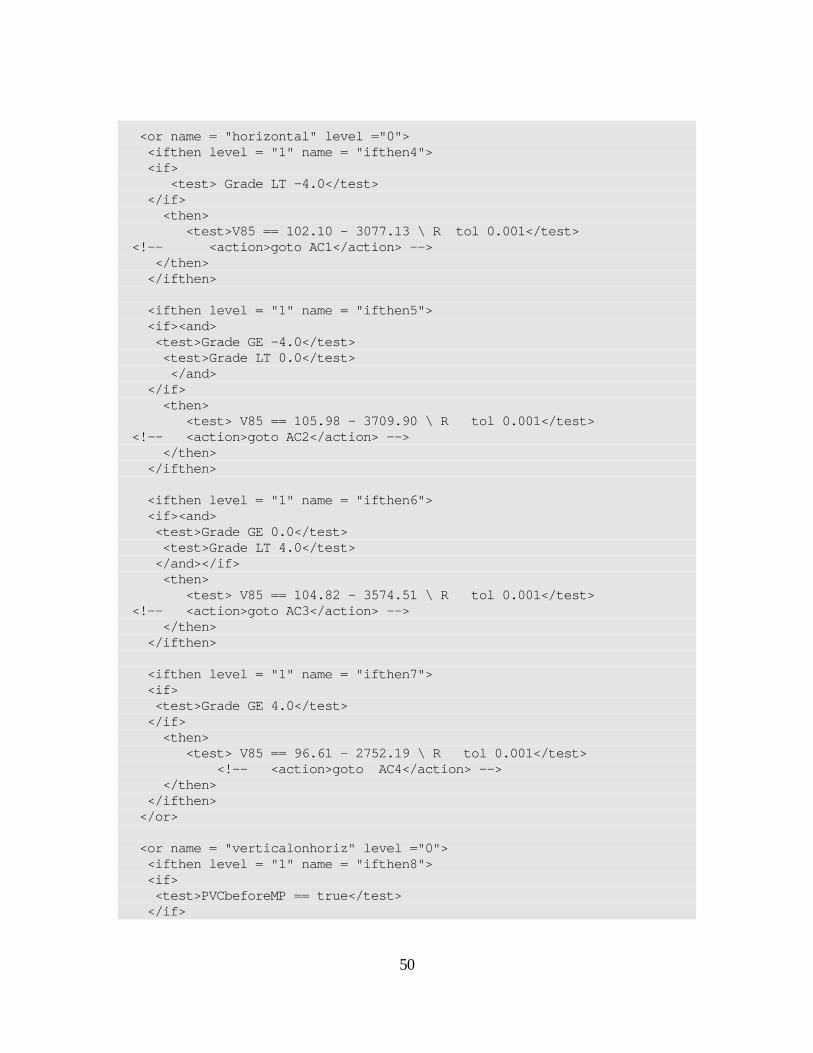
50
<or name = "horizontal" level ="0"> <ifthen level = "1" name = "ifthen4"> <if> <test> Grade LT -4.0</test> </if> <then> <test>V85 == 102.10 - 3077.13 \ R tol 0.001</test> <!-- <action>goto AC1</action> --> </then> </ifthen> <ifthen level = "1" name = "ifthen5"> <if><and> <test>Grade GE -4.0</test> <test>Grade LT 0.0</test> </and> </if> <then> <test> V85 == 105.98 - 3709.90 \ R tol 0.001</test> <!-- <action>goto AC2</action> --> </then> </ifthen> <ifthen level = "1" name = "ifthen6"> <if><and> <test>Grade GE 0.0</test> <test>Grade LT 4.0</test> </and></if> <then> <test> V85 == 104.82 - 3574.51 \ R tol 0.001</test> <!-- <action>goto AC3</action> --> </then> </ifthen> <ifthen level = "1" name = "ifthen7"> <if> <test>Grade GE 4.0</test> </if> <then> <test> V85 == 96.61 - 2752.19 \ R tol 0.001</test> <!-- <action>goto AC4</action> --> </then> </ifthen> </or> <or name = "verticalonhoriz" level ="0"> <ifthen level = "1" name = "ifthen8"> <if> <test>PVCbeforeMP == true</test> </if>
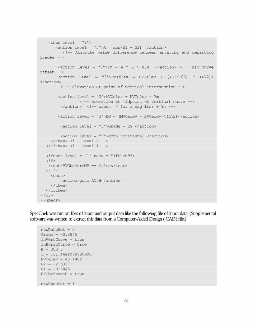
51
<then level = "2"> <action level = "3">A = abs(G1 - G2) </action> <!-- Absolute value difference between entering and departing grades --> <action level = "3">Ym = A * L \ 800 </action> <!-- mid-curve offset --> <action level = "3">PVIelev = PVCelev + ((G1\100) * (L\2)) </action> <!-- elevation at point of vertical intersection --> <action level = "3">MVCelev = PVIelev - Ym <!-- elevation at midpoint of vertical curve --> </action> <!-- crest - for a sag its: + Ym --> <action level = "3">EG = (MVCelev - PVCelev)\(L\2)</action> <action level = "3">Grade = EG </action> <action level = "3">goto horizontal </action> </then> <!-- level 2 --> </ifthen> <!-- level 1 --> <ifthen level = "1" name = "ifthen9"> <if> <test>PVCbeforeMP == false</test> </if> <then> <action>goto AC5B</action> </then> </ifthen> </or> </specs>
SpecChek was run on files of input and output data like the following file of input data. (Supplemental software was written to extract this data from a Computer-Aided Design ( CAD) file.)
newDataSet = 0 Grade = -0.3845 inVertCurve = true inHorizCurve = true R = 300.0 L = 161.44419999999997 PVCelev = 43.1482 G2 = -2.5367 G1 = -0.3845 PVCbeforeMP = true newDataSet = 1
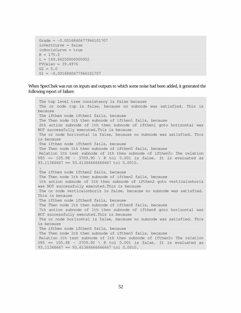
52
Grade = -0.0016840677966101707 inVertCurve = false inHorizCurve = true R = 175.0 L = 149.66250000000002 PVCelev = 39.4976 G2 = 0.0 G1 = -0.0016840677966101707
When SpecChek was run on inputs and outputs to which some noise had been added, it generated the following report of failure:
The top level tree consistency is false because The or node top is false, because no subnode was satisfied. This is because The ifthen node ifthen1 fails, because The Then node 1th then subnode of ifthen1 fails, because 2th action subnode of 1th then subnode of ifthen1 goto horizontal was NOT successfully executed.This is because The or node horizontal is false, because no subnode was satisfied. This is because The ifthen node ifthen5 fails, because The Then node 1th then subnode of ifthen5 fails, because Relation 1th test subnode of 1th then subnode of ifthen5: The relation V85 == 105.98 - 3709.90 \ R tol 0.001 is false. It is evaluated as 93.11366667 == 93.61366666666667 tol 0.0010. . The ifthen node ifthen2 fails, because The Then node 1th then subnode of ifthen2 fails, because 1th action subnode of 1th then subnode of ifthen2 goto verticalonhoriz was NOT successfully executed.This is because The or node verticalonhoriz is false, because no subnode was satisfied. This is because The ifthen node ifthen8 fails, because The Then node 1th then subnode of ifthen8 fails, because 7th action subnode of 1th then subnode of ifthen8 goto horizontal was NOT successfully executed.This is because The or node horizontal is false, because no subnode was satisfied. This is because The ifthen node ifthen5 fails, because The Then node 1th then subnode of ifthen5 fails, because Relation 1th test subnode of 1th then subnode of ifthen5: The relation V85 == 105.98 - 3709.90 \ R tol 0.001 is false. It is evaluated as 93.11366667 == 93.61366666666667 tol 0.0010.
53
Chapter 7 Numerical Reliability
This chapter presents a method for computing the maximum and expected error in a numerical computation.
Framework Reference
The framework used here for analyzing errors in a floating point number system appears in Nicholas J. Higham’s Accuracy and Stability of Numerical Algorithms.(9)
Errors in a Single Arithmetic Operation
Floating Point Number Systems
Floating point numbers, broadly defined to include the various sizes (such as double precision) are represented in the computer as ±0d1d2…dt Be where
B is the base of the number system. This is usually 2 for the computer’s internal arithmetic and 10 for numbers printed or displayed for human beings.
d1,...,dt are integers in the range
Bdi <≤0
01≠d
The precision of the number system is t. eB is B to the eth power. e is an integer in some finite interval around 0. Usually the range of e is
defined as follows (for some positive integer m):
For typical double precision numbers written to the base 10:
The precision t = 15
The range of exponent for 10 is ±308.
The Range of a Floating Point Number System
Note that in contrast to numbers in pure mathematics, there are numbers that cannot be well

54
approximated in a particular floating point number system. For a typical double precision number system,
±10±400
are outside the range of the number systems.
Approximation of Real Numbers by Floating Point Numbers
In studying numerical approximations, an important quantity is the relative error of the floating point approximation to the pure mathematical number. Let fl(x) stand for the floating point approximation of x. Then the relative error is defined as
For a number x inside the number system, the relative approximation error
is a small number, while for numbers outside the number system this number may be very large. In fact, Higham shows that for numbers in the range of a floating point number system,(9)
Where
Where B is the base of number system, and t is the precision, i.e., the number of digits in the mantissa.
Intuitively, the correctness of Higham’s formula for u can be demonstrated in the following way: Let d0.d1...dt-1Ep be a number in scientific notation, where d0 is the digit in front of the decimal, d1 through dt-1 are the digits to the right of the decimal, and p is a power of 10. This number has t digits in the mantissa, just like Higham’s floating point numbers. The error in the mantissa of the number in scientific notation is up to 5*10-t, which is
( )x
xxflxRErr
−=)(
for a pure mathematical number 0≠x .
(17)
( )x
xxfl −(18)
( ) uxRErr ≤ (19)
( )
22
1 tt BBBu
−− =∗= (20)
( ) ( )tt −−− ∗=∗ 11 102110
21
(21)

55
For the typical double precision arithmetic in decimal notation (B == 10), t = 15, so:
Errors in Floating Point Operations
For theoretical analysis of errors, it is assumed that an arithmetic operation is implemented as well as it can be in floating point arithmetic, i.e., if op is one of the four arithmetic operations +, –, *, /,
Where x and y are pure mathematical numbers.
Errors as Random Variables
The above formula for relative error is equivalent to
a form more convenient in analyzing errors. To further simplify the representation of error, it is convenient to introduce a random variable, e, in the interval ±u. For a particular real number or operation, the precise value of e is not usually known, so using a random variable is reasonable. However, Higham presents examples in which errors are not random. For the most part, it is assumed that e is uniformly distributed over the interval ±u, but this general-purpose assumption may not hold for particular computations. Using the random variable, the last inequality can be written as
Higham also proves another convenient error bound,
For a uniform random variable, over an interval of length d, the variance is
15105 −∗=u (22)
( )( ) uyopxflRErr ≤ (23)
( ) ( )( )uyopxyopxfl +≤ 1 (24)
fl(x op y) = (x op y)(1 + e) (25)
( ) ( )exxfl+
=1
(26)
12
2d
(27)

56
Therefore for e, the variance is
Pushing Errors through an Arithmetic Operation
Based on the above framework provided by Higham, it is possible to calculate, step by step, along with its value, the expected and maximum error of a computed number. This section shows that computer numbers, as defined above, are closed under the arithmetic operations. In addition, formulas are provided to compute the variances and maximum errors under arithmetic operations.
A Number Object for Error Analysis
Most numbers in the computer contain errors, either through measurement, roundoff, or both. (Exceptions are integers and some rational numbers from pure mathematics.) To characterize a number for error analysis, assume that the following are known:
• A point estimate of the number.
• The variance of the number.
• The maximum error of the number.
If x is a number, v(x) and me(x) denote the variance and maximum error of x. Also, fl(x) is the computed value of a number. While x denotes its theoretical value, t(x) also will be used to denote the theoretical value, where an explicit notation is needed. The computed and theoretical values differ by a random error, e(x).
( )12
2 2u∗
(28)

57
Random Expressions for Computational Errors
Addition
Table 1: Formula for Addition
What Why fl(a+b) = (1+e1)(fl(a)+fl(b)) 1. e1 is a random error introduced by
addition operation. 2. The computation is performed with computer approximations of a and b.
fl(a+b) = fl(a)+fl(b) + e1*(fl(a)+fl(b)) Algebra. fl(a)+fl(b) = t(a)(1+e(a)) + t(b)(1+e(b)) = t(a) + t(b) + t(a)*e(a)) + t(b)*e(b)
Substituting theoretical value + errors for computed value.
fl(a+b) = t(a) + t(b) + (fl(a)-e(a))*e(a)) + (fl(b)-e(b))*e(b) + e1*(fl(a)+fl(b))
Using definition of t(), fl() and e().
fl(a+b) = t(a) + t(b) + fl(a)*e(a) + fl(b)*e(b) + e1*(fl(a)+fl(b))
Throwing away higher powers of random variables.
This says that the computed value of the sum differs from the true value by a random expression
Note that the coefficients of the random variables are known, because fl(a) and fl(b) are the computer values corresponding to a and b.
Because
Where fabs is the absolute value function,
v(a) and v(b) are known, provided that the entire computation is carried out with the number objects defined above, containing a variance and maximum error in addition to a point value. v(e1) is also known, because e1 is a random variable on an interval of known size, namely 2*u:
(Note that when adding near opposites, the size of u can change, as discussed for subtraction below.) Therefore, the variance of a sum can be computed from the variance of its arguments up to an error by
fl(a)*e(a)) + fl(b)*e(b) + e1*(fl(a)+fl(b)) (29)
var(c1*e1+c2*e2) = fabs(c1)*var(e1) + fabs(c2)*var(e2) (30)
v(a+b) = fabs(fl(a))*v(a) + fabs(fl(b))*v(b) + fabs(fl(a)+fl(b))*v(e1) (31)
( ) ( )12
21
2uev
∗=
(32)
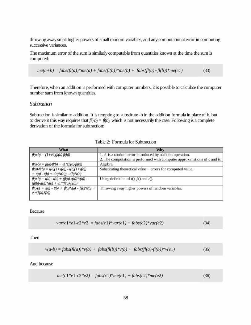
58
throwing away small higher powers of small random variables, and any computational error in computing successive variances.
The maximum error of the sum is similarly computable from quantities known at the time the sum is computed:
Therefore, when an addition is performed with computer numbers, it is possible to calculate the computer number sum from known quantities.
Subtraction
Subtraction is similar to addition. It is tempting to substitute -b in the addition formula in place of b, but to derive it this way requires that fl(-b) = fl(b), which is not necessarily the case. Following is a complete derivation of the formula for subtraction:
Table 2: Formula for Subtraction What Why
fl(a-b) = (1+e1)(fl(a)-fl(b)) 1. e1 is a random error introduced by addition operation. 2. The computation is performed with computer approximations of a and b.
fl(a-b) = fl(a)-fl(b) + e1*(fl(a)-fl(b)) Algebra. fl(a)-fl(b) = t(a)(1+e(a)) - t(b)(1+e(b)) = t(a) - t(b) + t(a)*e(a)) - t(b)*e(b)
Substituting theoretical value + errors for computed value.
fl(a-b) = t(a) - t(b) + (fl(a)-e(a))*e(a)) - (fl(b)-e(b))*e(b) + e1*(fl(a)-fl(b))
Using definition of t(), fl() and e().
fl(a-b) = t(a) - t(b) + fl(a)*e(a) - fl(b)*e(b) + e1*(fl(a)-fl(b))
Throwing away higher powers of random variables.
Because
Then
And because
me(a+b) = fabs(fl(a))*me(a) + fabs(fl(b))*me(b) + fabs(fl(a)+fl(b))*me(e1) (33)
var(c1*e1-c2*e2 = fabs(c1)*var(e1) + fabs(c2)*var(e2) (34)
v(a-b) = fabs(fl(a))*v(a) + fabs(fl(b))*v(b) + fabs(fl(a)-fl(b))*v(e1) (35)
me(c1*e1-c2*e2) = fabs(c1)*me(e1) + fabs(c2)*me(e2) (36)

59
Then
Loss of Precision in Subtracting Nearly Equal Numbers
Subtracting nearly equal quantities, or adding near opposites, causes the range of the random variable e(a) to expand. This is due to a loss of precision in a-b. This lack of precision is, in turn, due to the fact that only a small number of digits in a and b are different. Only these different digits appear in a-b. The range of the random error in doing an operation depends on the number of digits in the mantissa of the answer. When this is small, the range of the random variable increases.
Let
And likewise for b, for binary digits di, exponent e, and number system base B. If e and d1...dk are equal for both a and b, there are only t-k digits that differ in the two numbers. Therefore, there are only t-k digits in the mantissa of fl(a-b) that result from the subtraction of the mantissas of a and b. The range of e1 in this case is
Instead of
The number of agreeing digits k in the above formula can be found by bit fiddling on the computer representations of fl(a) and fl(b). Assuming as above that the mantissa bits are numbered from 1 to t, with bit 1 the most significant, let b(i,x) be the ith bit of the mantissa of x.
me(a-b) = fabs(fl(a))*me(a) + fabs(fl(b))*me(b) + fabs(fl(a)-fl(b))*me(e1) (37)
eBdtdda ∗= ...21.0 (38)
( )ktBu −−∗⎟⎠⎞
⎜⎝⎛=± 1
21' (39)
tBu −∗⎟⎠⎞
⎜⎝⎛=± 1
21
(40)

60
Then
int effective_mantissa_length( fl(a), fl(b)) { int t = length(mantissa(a)); // assume that also t = length(mantissa(b)) if (exponent(fl(a)) != exponent(fl(b))) return t; int i = 1; while ( t>=0 && i<=t) { if (b(i,a)==b(i,b) t--; else return t; i++; } return t; }
We can also find the number of agreeing digits with good accuracy by computing the minimum, for a and b of integer part log(base B)(fabs(c)/fabs(a-b)), where c in {a, b} and B is the base of the computer number system.
This computation of the range of the random variable e1 should be done for all subtraction operations where the arguments are nearly equal and all addition operations where they are nearly equal in magnitude but differ in sign.
The Effect of Errors in Computing Integer Part log(base B)(fabs(c)/fabs(a-b))
Note that there is some error in computing log(base B)(fabs(c)/fabs(a-b)). However, this error only matters when it causes a value to cross an integer boundary erroneously. Because the error is a multiple of the precision of computer arithmetic, it is small number, so only logs in a narrow interval around integers are susceptible to this error. Therefore, an error in computing integer part log(base B)(fabs(c)/fabs(a-b)) is possible but rare. Because the total computational error is generally a sum of a large number of random variables, and because higher order terms already are thrown away, the usually small estimation error caused by errors in integer part log(base B)(fabs(c)/fabs(a-b)) will be ignored.

61
Multiplication
Table 3: Formula for Multiplication
What Why fl(a*b) = (1+e1)*fl(a)*fl(b) 1. e1 is a random error introduced by multiplication operation.
2. The computation is performed with computer approximations of a and b.
fl(a*b) = fl(a)*fl(b) + e1*fl(a)*fl(b) Algebra. fl(a)*fl(b) = t(a)*(1+e(a)) * t(b)*(1+e(b)) = t(a)*t(b)*(1+e(a)+e(b)+e(a)*e(b))
Substituting theoretical value + errors for computed value.
fl(a)*fl(b) = t(a)*(1+e(a)) * t(b)*(1+e(b)) = t(a)*t(b)*(1+e(a)+e(b)) = t(a)*t(b) +t(a)*t(b)*(e(a)+e(b))
Throwing away terms in higher powers of random variables, because these terms are much smaller than the others, given the typical precision for computer arithmetic.
t(a)*t(b) = (fl(a)-e(a))*(fl(b)-e(b)) = fl(a)*fl(b) - e(a)*fl(b) - e(b)*fl(a) + e(a)*e(b) = fl(a)*fl(b) - e(a)*fl(b) - e(b)*fl(a)
To express the random expression in terms of computationally known quantities, rewrite t(a)*t(b) in terms of fl(a) and fl(b), and throw away small terms.
fl(a*b) = t(a)*t(b) +(fl(a)*fl(b) - e(a)*fl(b) - e(b)*fl(a)) *(e(a)+e(b)) + e1*fl(a)*fl(b) = t(a)*t(b) +fl(a)*fl(b)*(e1+e(a)+e(b))
Substituting for t(a)*t(b), simplifying, and throwing away small terms.
Then
and
This describes the random expression for the error in multiplication in terms of coefficients and random variables, where the coefficients, means, and variances of the random variables are known when the multiplication is performed.
var(a*b) = fabs(fl(a)*fl(b)) *( var(e1) + var(e(a)) + var(e(b))) (41)
me(a*b) = fabs(fl(a)*fl(b)) *( me(e1) + me(e(a)) + me(e(b))) (42)
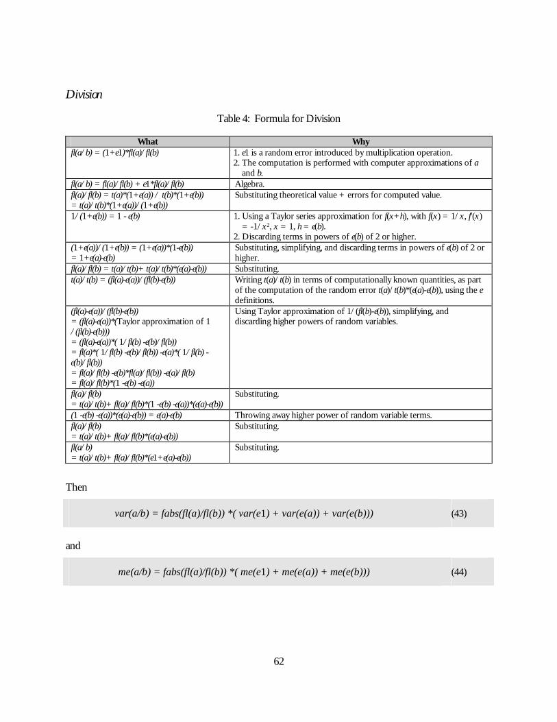
62
Division
Table 4: Formula for Division
What Why fl(a/b) = (1+e1)*fl(a)/fl(b) 1. e1 is a random error introduced by multiplication operation.
2. The computation is performed with computer approximations of a and b.
fl(a/b) = fl(a)/fl(b) + e1*fl(a)/fl(b) Algebra. fl(a)/fl(b) = t(a)*(1+e(a)) / t(b)*(1+e(b)) = t(a)/t(b)*(1+e(a))/(1+e(b))
Substituting theoretical value + errors for computed value.
1/(1+e(b)) = 1 - e(b) 1. Using a Taylor series approximation for f(x+h), with f(x) = 1/x, f'(x) = -1/x2, x = 1, h = e(b).
2. Discarding terms in powers of e(b) of 2 or higher. (1+e(a))/(1+e(b)) = (1+e(a))*(1-e(b)) = 1+e(a)-e(b)
Substituting, simplifying, and discarding terms in powers of e(b) of 2 or higher.
fl(a)/fl(b) = t(a)/t(b)+ t(a)/t(b)*(e(a)-e(b)) Substituting. t(a)/t(b) = (fl(a)-e(a))/(fl(b)-e(b)) Writing t(a)/t(b) in terms of computationally known quantities, as part
of the computation of the random error t(a)/t(b)*(e(a)-e(b)), using the e definitions.
(fl(a)-e(a))/(fl(b)-e(b)) = (fl(a)-e(a))*(Taylor approximation of 1 /(fl(b)-e(b))) = (fl(a)-e(a))*( 1/fl(b) -e(b)/fl(b)) = fl(a)*( 1/fl(b) -e(b)/fl(b)) -e(a)*( 1/fl(b) -e(b)/fl(b)) = fl(a)/fl(b) -e(b)*fl(a)/fl(b)) -e(a)/fl(b) = fl(a)/fl(b)*(1 -e(b) -e(a))
Using Taylor approximation of 1/(fl(b)-e(b)), simplifying, and discarding higher powers of random variables.
fl(a)/fl(b) = t(a)/t(b)+ fl(a)/fl(b)*(1 -e(b) -e(a))*(e(a)-e(b))
Substituting.
(1 -e(b) -e(a))*(e(a)-e(b)) = e(a)-e(b) Throwing away higher power of random variable terms. fl(a)/fl(b) = t(a)/t(b)+ fl(a)/fl(b)*(e(a)-e(b))
Substituting.
fl(a/b) = t(a)/t(b)+ fl(a)/fl(b)*(e1+e(a)-e(b))
Substituting.
Then
and
var(a/b) = fabs(fl(a)/fl(b)) *( var(e1) + var(e(a)) + var(e(b))) (43)
me(a/b) = fabs(fl(a)/fl(b)) *( me(e1) + me(e(a)) + me(e(b))) (44)

63
Computing Errors for an Entire Computation
As seen in the previous section, for each of the four arithmetic operations, the random error in a computed number is approximated by a linear sum of random variables. In this linear sum, the coefficients and the variances of the random variables are known at the time the arithmetic operation is performed. The linear sum approximates the true random expression up to random variable terms containing squares or higher powers of random variables. Because all the random variables have ranges of 1E-7 for floating point, or 1E-15 for double precision, these higher power terms are much smaller than the linear terms, and so can be safely discarded.
Given this, the maximum error and the standard error for a computed number can be computed as follows: First, order the inputs, intermediate results, and final results so that the inputs to each arithmetic operation appear in the list before the result of the operation. Now the point estimate, variance, and maximum error of each number in the list will be computed in turn.
For measurement inputs to a computation, begin with the measurement (as a point estimate), the measurement’s variance, and the maximum error of the measurement.
For a computed number in the list, let the number be computed by
a op b Where the random expression for op is c1*e(a) + c2*e(b) * c3*e1, where
• The c values are known coefficients (from the formulas of the previous section).
• e(a) and e(b) are the random errors of the inputs to the operation. The point estimates of a and b and their variances and maximum errors are assumed to be known.
Then the variance of a op b is
Where fabs is the absolute value function. The maximum error is
Given that there are a finite number of steps in a computation, repeated application of these formulas produces the maximum error and variance of the final result. (See appendix B for an example of errors in large sums.)
fabs(c1)*var(e(a))+fabs(c2)*var(e(b))+ fabs(c3)*var(e1) (45)
fabs(c1)*me(e(a))+fabs(c2)*me(e(b))+ fabs(c3)*me(e1) (46)


65
Chapter 8 Tools for Software Reliability
This chapter contains information and resources for software development tools. Some of these tools are directly useful to FHWA. Others (currently applied to non-highway topics) may potentially improve the highway software development process.
Resources
The following organizations examine software correctness issues and provide useful information on their Web sites:
• The National Institute of Standards and Technology (NIST) Software Quality Group (http://hissa.nist.gov). The NIST Software Quality Group maintains several useful software engineering knowledge bases, including the Dictionary of Algorithms, Data Structures, and Problems.
• Software Engineering Body of Knowledge (SWEBOK). http://www.swebok.org/
• Center for High Assurance Computer Systems, Naval Research Laboratory (NRL). http://chacs.nrl.navy.mil
• The Center for High Assurance Computer Systems. The center is a branch within the Information Technology Division of the NRL (http://chacs.nrl.navy.mil).
• The Software Engineering Institute (SEI). SEI is a federally funded research and development center sponsored by the U.S. Department of Defense (DoD) (http://www.sei.cmu.edu/). o To a large degree, SEI has focused on the process of developing software. Featured are the
Capability Maturity Models®:
− Capability Maturity Model for Software (SW-CMM).
− People Capability Maturity Model (P-CMM).
− Software Acquisition Capability Maturity Model (SA-CMM).
− Systems Engineering Capability Maturity Model (SE-CMM).
− Integrated Product Development Capability Maturity Model (IPD-CMM).
o Additional SEI processes for software development include the Personal Software Process and the Team Software Process (see http://www.sei.cmu.edu/tsp).
o SEI has detailed good engineering practices throughout the software life cycle (see http://www.sei.cmu.edu/engineering/engineering.html). Of particular interest:

66
− Methods for representing system architecture. The goal of these methods is to capture important system properties in an understandable form. (http://www.sei.cmu.edu/ata/arch_rep.html).
− The SEI Repository (SEIR). SEIR provides a forum for contributing and exchanging information concerning software engineering improvement activities (http://seir.sei.cmu.edu/seir/frames/frmset.help.asp).
o Because SEI’s methods were developed for DoD, some are not practical for the lower budget, more decentralized environments of highway software development.
Tools
The Software Engineering Laboratory of the Department of Computing, Imperial College of Science, Technology and Medicine, University of London, maintains a list of software development tools (http://www-dse.doc.ic.ac.uk:80/sel/tools_env.html), with descriptions and links for each.
The following tools may be useful in the software development process:
• DOORS (http://www.telelogic.com/products/doorsers/doors/index.cfm)is a GUI-based requirements engineering environment that helps manage requirements throughout development life cycles. Requirements are handled within DOORS as discrete objects. Each requirement can be tagged with an unlimited number of attributes (text, integer, Boolean, real, date, enumerations, etc.) to allow easy selection of subsets of requirements for specialist tasks. DOORS appears to be useful for keeping the requirements for large projects organized and tracking their implementation through the software life cycle.
• Rational Rose (http://www.rational.com) is a collection of Computer-Aided Software Engineering (CASE) tools for object-oriented design, including a tool called visual modeling, which produces diagrams that describe the content of classes in object oriented designs, and the relationship between the classes.
• Table Tool System (TTS) (http://www.crl.mcmaster.ca/SERG/TTS/ttsHome.html) is a set of tools for creating, verifying, and testing tabular specifications, i.e., tables of mathematical expressions representing software specifications.
In addition to the tools listed above, the Imperial College list contains examples of:
• Tools that exclusively produce drawings to describe systems.
• Tools based on formal languages such as Z, in which writing the formal specifications appears harder than coding the system itself.
• Tools based on finite-state models, where translating specifications into the finite-state model appears error-prone.

67
Appendix A
Wrapping Source Code The following is the output produced by running the source code provided in chapter 6, Wrapping the Integer Factorial.
Run of Integer Factorial
This is a run of a recursive factorial using integers in C.
Enter an integer: 8 asking for fact(7) asking for fact(6) asking for fact(5) asking for fact(4) asking for fact(3) asking for fact(2) asking for fact(1) j=1, fact(j) = 1 j=2, fact(j) = 2 j=3, fact(j) = 6 j=4, fact(j) = 24 j=5, fact(j) = 120 j=6, fact(j) = 720 j=7, fact(j) = 5040 j=8, fact(j) = -25216

68
Run of Wrapped Factorial
This is a run of a recursive factorial with wrapping (wrap_fact(8)) using integers in C.
asking for fact(7) asking for fact(6) asking for fact(5) asking for fact(4) asking for fact(3) asking for fact(2) asking for fact(1) j=1, fact(j) = 1 j=2, fact(j) = 2 j=3, fact(j) = 6 j=4, fact(j) = 24 j=5, fact(j) = 120 j=6, fact(j) = 720 j=7, fact(j) = 5040 asking for ffact(7) asking for ffact(6) asking for ffact(5) asking for ffact(4) asking for ffact(3) asking for ffact(2) asking for ffact(1)c j=1, ffact(j) = 1.000000 j=2, ffact(j) = 2.000000 j=3, ffact(j) = 6.000000 j=4, ffact(j) = 24.000000 j=5, ffact(j) = 120.000000 j=6, ffact(j) = 720.000000 j=7, ffact(j) = 5040.000000 Inside wrapped_fact, arg = 8, *flag=0
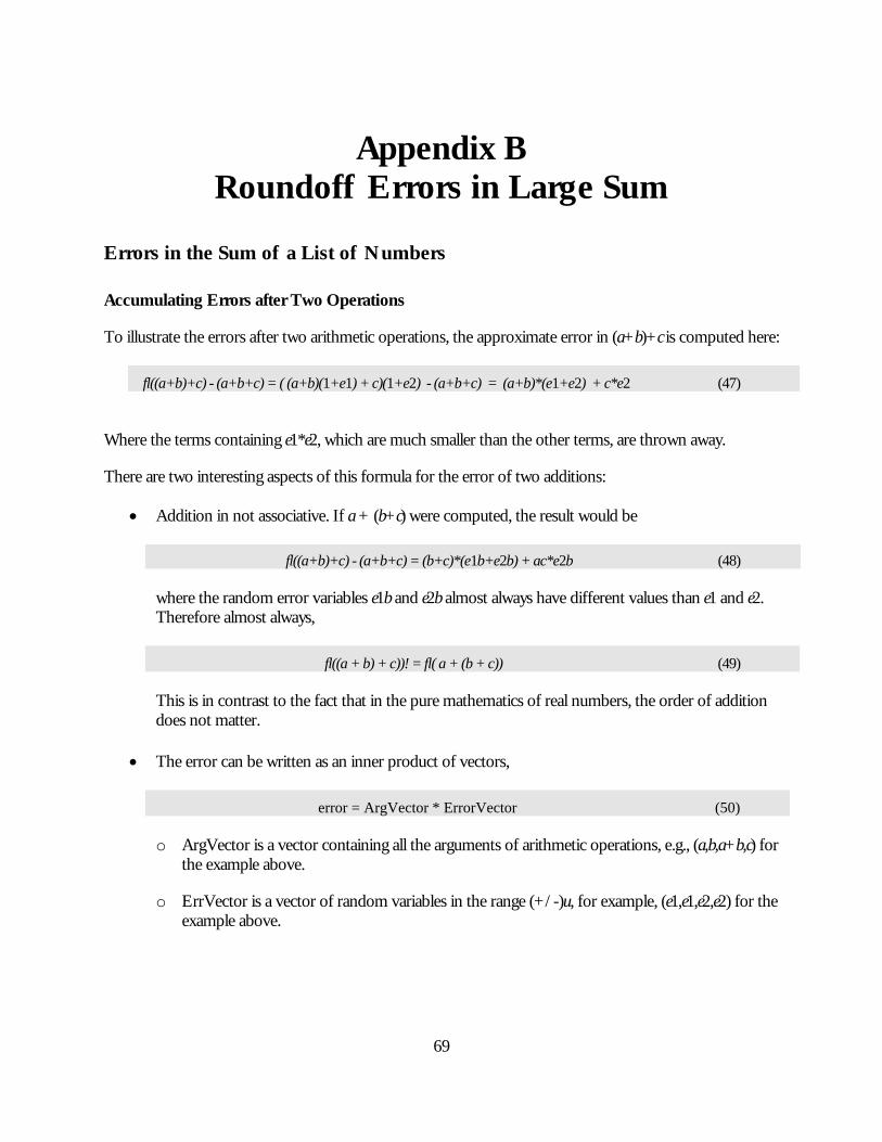
69
Appendix B
Roundoff Errors in Large Sum
Errors in the Sum of a List of Numbers
Accumulating Errors after Two Operations
To illustrate the errors after two arithmetic operations, the approximate error in (a+b)+c is computed here:
fl((a+b)+c) - (a+b+c) = ( (a+b)(1+e1) + c)(1+e2) - (a+b+c) = (a+b)*(e1+e2) + c*e2 (47) Where the terms containing e1*e2, which are much smaller than the other terms, are thrown away.
There are two interesting aspects of this formula for the error of two additions:
• Addition in not associative. If a + (b+c) were computed, the result would be
fl((a+b)+c) - (a+b+c) = (b+c)*(e1b+e2b) + ac*e2b (48) where the random error variables e1b and e2b almost always have different values than e1 and e2. Therefore almost always,
fl((a + b) + c))! = fl( a + (b + c)) (49) This is in contrast to the fact that in the pure mathematics of real numbers, the order of addition does not matter.
• The error can be written as an inner product of vectors,
error = ArgVector * ErrorVector (50)
o ArgVector is a vector containing all the arguments of arithmetic operations, e.g., (a,b,a+b,c) for the example above.
o ErrVector is a vector of random variables in the range (+/-)u, for example, (e1,e1,e2,e2) for the example above.
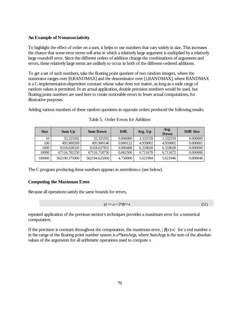
70
An Example of Nonassociativity
To highlight the effect of order on a sum, it helps to use numbers that vary widely in size. This increases the chance that some error terms will arise in which a relatively large argument is multiplied by a relatively large roundoff error. Since the different orders of addition change the combinations of arguments and errors, these relatively large terms are unlikely to occur in both of the different-ordered additions.
To get a set of such numbers, take the floating point quotient of two random integers, where the numerator ranges over [0,RANDMAX] and the denominator over [1,RANDMAX], where RANDMAX is a C-implementation-dependent constant whose value does not matter, as long as a wide range of random values is permitted. In an actual application, double precision numbers would be used, but floating point numbers are used here to create noticeable errors in fewer actual computations, for illustrative purposes.
Adding various numbers of these random quotients in opposite orders produced the following results.
Table 5. Order Errors for Addition
Size Sum Up Sum Down Diff. Avg. Up Avg.
Down Diff/Size
10 33.325592 33.325592 0.000000 3.332559 3.332559 0.000000100 495.900269 495.900146 0.000122 4.959002 4.959002 0.000001
1000 6318.028320 6318.027832 0.000488 6.318028 6.318028 0.00000010000 67116.781250 67116.718750 0.062500 6.711678 6.711672 0.000006
100000 562199.375000 562194.625000 4.750000 5.621994 5.621946 0.000048
The C program producing these numbers appears in averrdemo.c (see below).
Computing the Maximum Error
Because all operations satisfy the same bounds for errors,
|e| <= u = 5*B^ -̂t (51) repeated application of the previous section’s techniques provides a maximum error for a numerical computation.
If the precision is constant throughout the computation, the maximum error, |fl(x)-x| for a real number x in the range of the floating point number system is u*SumArgs, where SumArgs is the sum of the absolute values of the arguments for all arithmetic operations used to compute x.

71
This maximum error can be computed along with x, because:
• u is a known quantity for any particular floating point number system and, in particular, has the value 5E-15 for the typical double precision operation.
• SumArgs can be calculated as a running sum during the computation of x.
Computing the Probable Error
While the small random error variables need not be random, they often behave so, and the observed error is much smaller than the maximum error. Therefore, it is useful to assume that the actual error is a weighted sum of random error variables and to compute the standard deviation of the error.
Assuming that the distribution of errors is uniform over a u radius interval around zero, the actual error is a weighted sum of the random error variables (the e’s). Under reasonable assumptions about the probability density functions for the individual e’s, such as assuming a uniform distribution of errors in the u interval, the Central Limit Theorem applies.
For e distributions for which the Central Limit Theorem applies, such as a uniform distribution for each of the e’s:
• The best point estimate of the error is 0. This is because the expected error is the weighted sum of the means of the individual error distributions. This is 0, because each of the individual e’s is assumed to have a mean of 0.
• The variance is the weighted sum of the variances of the individual e’s. If each e is a uniform random variable on [-u,u], each has a variance of (2*u)^^2/12. The variance of the error entire computation is then SumArgs*(2*u)^^2/12.
Application: Adding N Numbers
To add, in order N, floating point numbers that are:
• All non-negative (so the example is not complicated with estimates of precision of intermediate results).
• About the same size, to enable some approximations shown below.
In this case, the intermediate results are:
• The N numbers themselves.
• The partial sums of the first k numbers, from k = 2 to k = n.
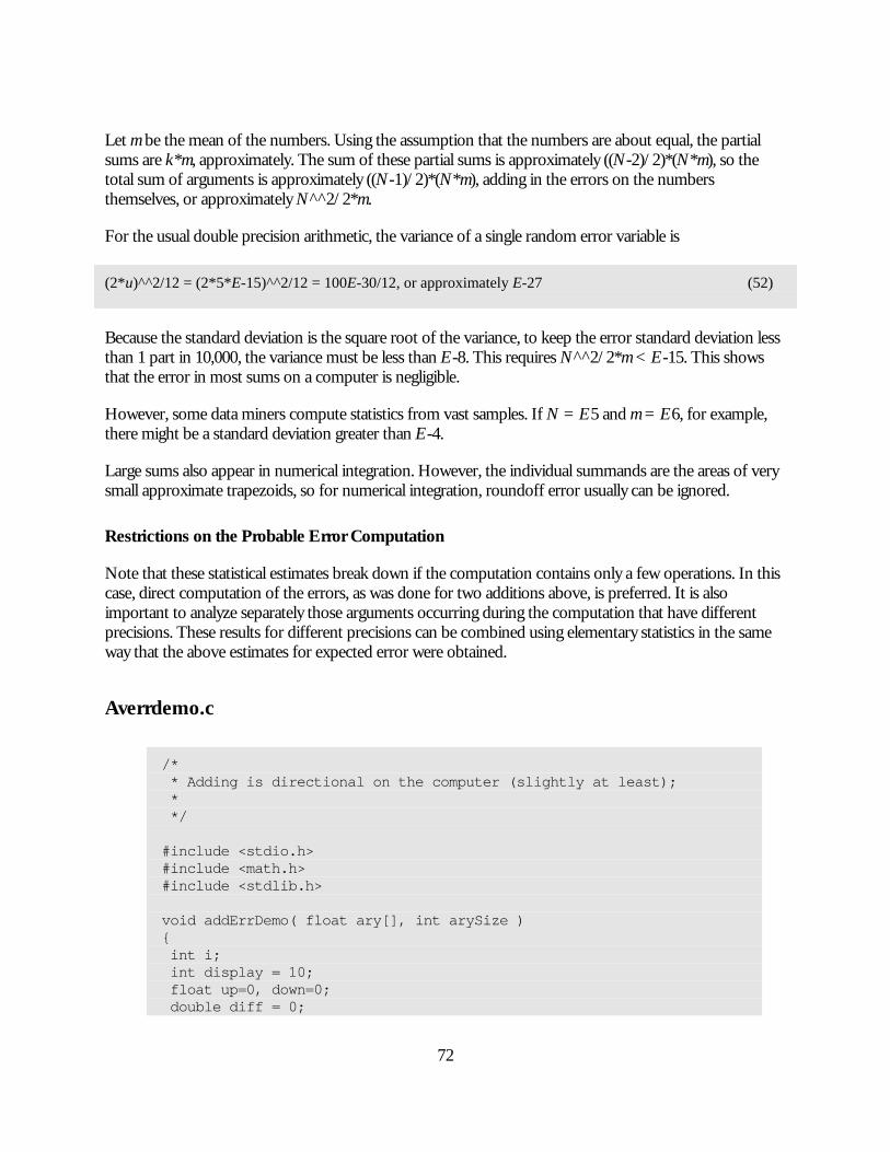
72
Let m be the mean of the numbers. Using the assumption that the numbers are about equal, the partial sums are k*m, approximately. The sum of these partial sums is approximately ((N-2)/2)*(N*m), so the total sum of arguments is approximately ((N-1)/2)*(N*m), adding in the errors on the numbers themselves, or approximately N^^2/2*m.
For the usual double precision arithmetic, the variance of a single random error variable is
(2*u)^^2/12 = (2*5*E-15)^^2/12 = 100E-30/12, or approximately E-27 (52) Because the standard deviation is the square root of the variance, to keep the error standard deviation less than 1 part in 10,000, the variance must be less than E-8. This requires N^^2/2*m < E-15. This shows that the error in most sums on a computer is negligible.
However, some data miners compute statistics from vast samples. If N = E5 and m = E6, for example, there might be a standard deviation greater than E-4.
Large sums also appear in numerical integration. However, the individual summands are the areas of very small approximate trapezoids, so for numerical integration, roundoff error usually can be ignored.
Restrictions on the Probable Error Computation
Note that these statistical estimates break down if the computation contains only a few operations. In this case, direct computation of the errors, as was done for two additions above, is preferred. It is also important to analyze separately those arguments occurring during the computation that have different precisions. These results for different precisions can be combined using elementary statistics in the same way that the above estimates for expected error were obtained.
Averrdemo.c
/* * Adding is directional on the computer (slightly at least); * */ #include <stdio.h> #include <math.h> #include <stdlib.h> void addErrDemo( float ary[], int arySize ) { int i; int display = 10; float up=0, down=0; double diff = 0;

73
// populate ary for (i=0;i<arySize;i++) { int num, denom; num = rand(); denom = rand(); if (denom == 0) denom = 1; ary[i] = (float)num/(float)denom; if (i<display) { printf("ary[%d]=%f\n",i,ary[i]); } } for (i=0;i<arySize;i++) { up = up+ary[i]; down = down+ary[arySize - 1 - i]; } diff = fabs(up - down); printf("arySize = %d, up = %f, down = %f, diff = %f\n\n", arySize, up, down, diff); up = up / arySize; down = down / arySize; diff = diff / arySize; printf("arySize = %d, av. up = %f, av. down = %f, diff/arySize = %f\n\n", arySize, up, down, diff); } int main(void) { char dummy = ' '; /* This defines an array of integers. */ float ary1[10]; float ary2[100]; float ary3[1000]; float ary4[10000]; float ary5[100000]; addErrDemo( ary1, 10); addErrDemo( ary2, 100); addErrDemo( ary3, 1000); addErrDemo( ary4, 10000); addErrDemo( ary5, 100000); return 0; }

74
Random Quotients
2.661538 10.075230 1.637769 2.742790 0.737261 0.618492 0.156082 13.597059 0.202537 0.896834 0.862536 0.514122 1.134683 1.138535 0.745811 1.103303 0.762726 0.280541 0.180905 0.967002 7.859444 0.627772 1.148473 1.121295 0.991399 0.175100 7.511935 2.012076 0.305450 0.499849 0.837121 0.439698 0.934848 1.341262 5.321136 0.005740 1.643820 1.454574 0.433644 4.145180 1.180458 0.859678 45.906124 0.575061 0.060546 0.156742 0.296229 0.428692

75
0.441928 0.318231


77
References 1. Musa, J.D., A. Iannino, and K. Okumoto. Software Reliability: Measurement, Prediction,
Application. McGraw Hill, 1987.
2. Leveson, N. Safeware, System Safety and Computers. Addison Wesley, 1995, ISBN 0-201-11972-2.
3. Wentworth, J. and R. Knaus. “Correctness Given Mathematical Specifications,” in Producing Correct Software, Turner Fairbank Highway Research Center, McLean, VA, 1999. (www.tfhrc.gov/advanc/softwar/soft2.htm), accessed January 2001.
4. Wallace, D.R., L.M. Ippolito, and B. Cuthill. Reference Information for the Software Verification and Validation Process, National Institute of Standards and Technology Special Publication 500-234, March 29, 1996. (http://hissa.nist.gov/HHRFdata/Artifacts/ITLdoc/234/val-proc.html).
5. Verification, Validation, and Evaluation of Expert Systems, an FHWA Handbook. Turner Fairbank Highway Safety Research Center, Federal Highway Administration, U.S. Department of Transportation, McLean, VA. (www.tfhrc.gov/advanc/vve/cover.htm), accessed July 27, 2000.
6. Landauer, C. and K.L. Bellman. “Constructed Complex Systems: Issues, Architectures and Wrappings,” pp. 233-38 in Proceedings EMCSR 96: Thirteenth European Meeting on Cybernetics and Systems Research, Symposium on Complex Systems Analysis and Design, 9–12 April 1996, Vienna, Austria. This is a paper about wrapping by the inventors of the concept.
7. Press, W., et al. Numerical Recipes in C. Cambridge University Press, 1992.
8. Instant Recall, Inc. SpecChek, www.irecall.com/specchek/SpecIndx.htm, SpecChek™ homepage, accessed July 27, 2000.
9. Higham, N.J. Accuracy and Stability of Numerical Algorithms, Society of Industrial and Applied Mathematics, Philadelphia, 1996, ISBN 0-89871-355-2. (The SIAM Web site is www.siam.org.)

79
Additional Resources Holloway, C.M. “What is Formal Methods?” http://atb-www.larc.nasa.gov/fm/fm-what.html, NASA Langley Formal Methods Team’s World-Wide Web pages, accessed February 17, 2001.
Neumann, P.G., moderator. http://catless.ncl.ac.uk/Risks, a Web-accessible posting of the Risks Forum, a monthly USENET newsletter about computer risks and failures, accessed July 27, 2000.
Neumann, P.G. Illustrative Risks to the Public in the Use of Computer Systems and Related Technology. (www.csl.sri.com/neumann/illustrative.html), accessed July 27, 2000.
Neumann, P.G. Illustrative Risks to the Public in the Use of Computer Systems, Commercial Aviation. (www.csl.sri.com/neumann/illustrative.html#9), accessed July 27, 2000.
Neumann, P.G. Illustrative Risks to the Public in the Use of Computer Systems, Rail, Bus, and Other Public Transit. (www.csl.sri.com/neumann/illustrative.html#10), accessed July 27, 2000.
Potter, B., J. Sinclair, and D. Till. An Introduction to Formal Specification and Z, 2nd edition, Prentice Hall International Series in Computer Science, Englewood Cliffs, NJ, 1996, ISBN 0-13-242207-7.
The Software Engineering Institute Web site, www.sei.cmu.edu/sei-home.html.
Wilkinson, J.H., Rounding Errors in Algebraic Processes. Notes on Applied Science, No. 32, Her Majesty’s Stationery Office, London, 1963. Also published by Prentice Hall, Englewood Cliffs, NJ, and Dover, NY, 1994, ISBN 0-486-67999-3.

HRDS-06/09-04(1M)ERecycledRecyclable