1

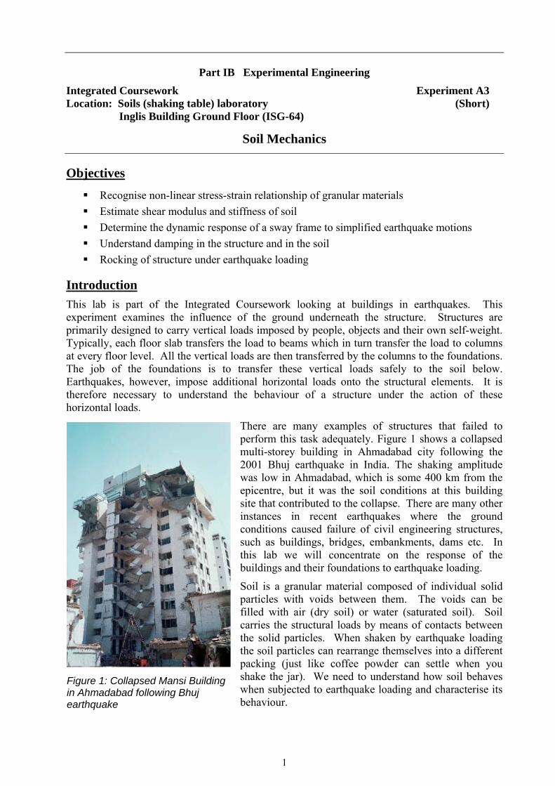
Figure 1: Collapsed Mansi Building in Ahmadabad following Bhuj earthquake

Part IB Experimental Engineering

Integrated Coursework Experiment A3 Location: Soils (shaking table) laboratory (Short) Inglis Building Ground Floor (ISG-64)

Soil Mechanics

Objectives

Recognise non-linear stress-strain relationship of granular materials

Estimate shear modulus and stiffness of soil

Determine the dynamic response of a sway frame to simplified earthquake motions

Understand damping in the structure and in the soil

Rocking of structure under earthquake loading

Introduction

This lab is part of the Integrated Coursework looking at buildings in earthquakes. This experiment examines the influence of the ground underneath the structure. Structures are primarily designed to carry vertical loads imposed by people, objects and their own self-weight. Typically, each floor slab transfers the load to beams which in turn transfer the load to columns at every floor level. All the vertical loads are then transferred by the columns to the foundations. The job of the foundations is to transfer these vertical loads safely to the soil below. Earthquakes, however, impose additional horizontal loads onto the structural elements. It is therefore necessary to understand the behaviour of a structure under the action of these horizontal loads.

There are many examples of structures that failed to perform this task adequately. Figure 1 shows a collapsed multi-storey building in Ahmadabad city following the 2001 Bhuj earthquake in India. The shaking amplitude was low in Ahmadabad, which is some 400 km from the epicentre, but it was the soil conditions at this building site that contributed to the collapse. There are many other instances in recent earthquakes where the ground conditions caused failure of civil engineering structures, such as buildings, bridges, embankments, dams etc. In this lab we will concentrate on the response of the buildings and their foundations to earthquake loading.

Soil is a granular material composed of individual solid particles with voids between them. The voids can be filled with air (dry soil) or water (saturated soil). Soil carries the structural loads by means of contacts between the solid particles. When shaken by earthquake loading the soil particles can rearrange themselves into a different packing (just like coffee powder can settle when you shake the jar). We need to understand how soil behaves when subjected to earthquake loading and characterise its behaviour.

2

Although soil is made up of solid particles and voids we can treat it, at a macroscopic level, as a continuum, and characterise its behaviour by means of bulk properties. For example, we can weigh a volume of sand and find out its average bulk unit weight. Similarly we can define the amount of void space in a soil sample as the void ratio e, equal to the ratio of the volume of voids to the volume of solid particles. Even the bulk stiffness of the soil can be measured as the settlement it suffers when subjected to an axial load (similar to the Young’s modulus for a solid material). Using these we can estimate the behaviour of the soil around the foundation.

Apparatus

This experiment consists of two parts. Everyone will do both parts, with a change about halfway through. In the first part, you will shake the same structure used throughout the Integrated Coursework and in IA Experiment 7, except this time it is on a box of soil. This part of the experiment looks at the dynamic behaviour of soil. The second part comprises an oedometer test to measure the static stiffness of the soil, which can then be related to the dynamic properties.

Shaking Table In the other IA/IB experiments on this structure, it was clamped to a rigid base. Here the structure is placed loosely on a 300mm deep sand bed which is then shaken with a shaking table (Figure 2). The structure is allowed to rock on the sand along with the raft (base) foundation. There are also additional accelerometers on this structure. One has been added to measure horizontal acceleration at the base (the input to the structure), and 2 accelerometers have been added to measure vertical accelerations of the base plate (Figure 3) to measure the rocking amplitude and frequency. The accelerometers on the 3 upper floors work as before.

The shaking table is used to shake a box of densely packed sand on top of which the structure is placed. It can produce shakes in the frequency range 0-5Hz, with amplitudes of up to 5mm. Because of the mechanism used, the shakes are not purely sinusoidal; this will be shown later when the table acceleration is analysed using a Fourier Transform (explained later in the handout).

It is worth noting another difference between this lab and IA Experiment 7 (vibration modes). The loading applied to the foundation and the structure in this lab is a transient loading, i.e., it is applied for a specific number of cycles. In contrast you used continuous harmonic loading in the IA lab. Note also that the model structure and foundation in this lab are free to vibrate in any mode, just like real structures in the field. Here we use simple near-sinusoidal shaking, even though real earthquakes inflict more complex shaking with multiple frequencies and directions. It is useful first to understand the response of the structure by using simpler inputs of given frequency.

Figure 2: The shaking table with the structure placed on top of a sand bed

Figure 3: The structure, with vertical accelerometers on the base

3

Oedometer

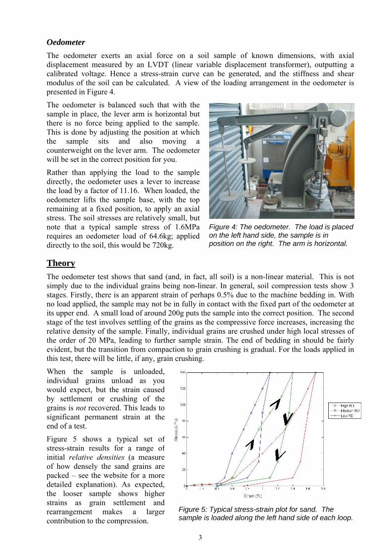
The oedometer exerts an axial force on a soil sample of known dimensions, with axial displacement measured by an LVDT (linear variable displacement transformer), outputting a calibrated voltage. Hence a stress-strain curve can be generated, and the stiffness and shear modulus of the soil can be calculated. A view of the loading arrangement in the oedometer is presented in Figure 4.

The oedometer is balanced such that with the sample in place, the lever arm is horizontal but there is no force being applied to the sample. This is done by adjusting the position at which the sample sits and also moving a counterweight on the lever arm. The oedometer will be set in the correct position for you.

Rather than applying the load to the sample directly, the oedometer uses a lever to increase the load by a factor of 11.16. When loaded, the oedometer lifts the sample base, with the top remaining at a fixed position, to apply an axial stress. The soil stresses are relatively small, but note that a typical sample stress of 1.6MPa requires an oedometer load of 64.6kg; applied directly to the soil, this would be 720kg.

Theory

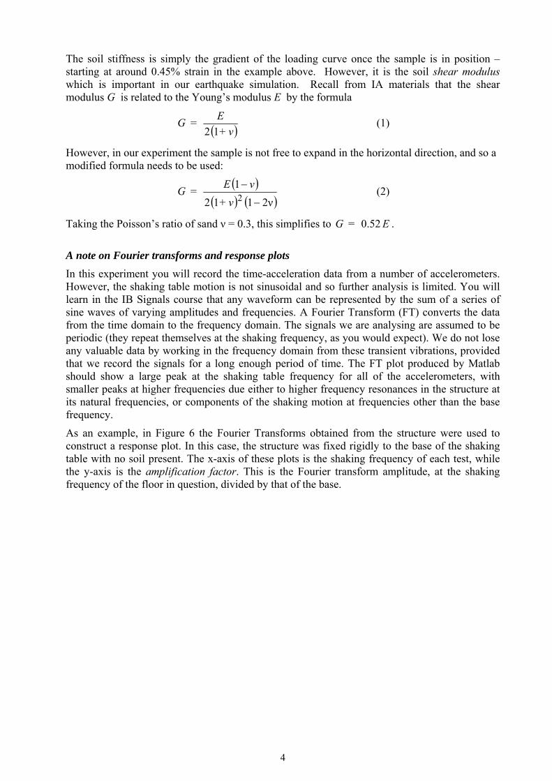
The oedometer test shows that sand (and, in fact, all soil) is a non-linear material. This is not simply due to the individual grains being non-linear. In general, soil compression tests show 3 stages. Firstly, there is an apparent strain of perhaps 0.5% due to the machine bedding in. With no load applied, the sample may not be in fully in contact with the fixed part of the oedometer at its upper end. A small load of around 200g puts the sample into the correct position. The second stage of the test involves settling of the grains as the compressive force increases, increasing the relative density of the sample. Finally, individual grains are crushed under high local stresses of the order of 20 MPa, leading to further sample strain. The end of bedding in should be fairly evident, but the transition from compaction to grain crushing is gradual. For the loads applied in this test, there will be little, if any, grain crushing.

When the sample is unloaded, individual grains unload as you would expect, but the strain caused by settlement or crushing of the grains is not recovered. This leads to significant permanent strain at the end of a test.

Figure 5 shows a typical set of stress-strain results for a range of initial relative densities (a measure of how densely the sand grains are packed – see the website for a more detailed explanation). As expected, the looser sample shows higher strains as grain settlement and rearrangement makes a larger contribution to the compression.

Figure 4: The oedometer. The load is placed on the left hand side, the sample is in position on the right. The arm is horizontal.

Figure 5: Typical stress-strain plot for sand. The sample is loaded along the left hand side of each loop.

4

The soil stiffness is simply the gradient of the loading curve once the sample is in position – starting at around 0.45% strain in the example above. However, it is the soil shear modulus which is important in our earthquake simulation. Recall from IA materials that the shear modulus G is related to the Young’s modulus E by the formula

ν+

E=G

12 (1)

However, in our experiment the sample is not free to expand in the horizontal direction, and so a modified formula needs to be used:

2ν112

12

ν+

νE=G (2)

Taking the Poisson’s ratio of sand ν = 0.3, this simplifies to E=G 52.0 .

A note on Fourier transforms and response plots

In this experiment you will record the time-acceleration data from a number of accelerometers. However, the shaking table motion is not sinusoidal and so further analysis is limited. You will learn in the IB Signals course that any waveform can be represented by the sum of a series of sine waves of varying amplitudes and frequencies. A Fourier Transform (FT) converts the data from the time domain to the frequency domain. The signals we are analysing are assumed to be periodic (they repeat themselves at the shaking frequency, as you would expect). We do not lose any valuable data by working in the frequency domain from these transient vibrations, provided that we record the signals for a long enough period of time. The FT plot produced by Matlab should show a large peak at the shaking table frequency for all of the accelerometers, with smaller peaks at higher frequencies due either to higher frequency resonances in the structure at its natural frequencies, or components of the shaking motion at frequencies other than the base frequency.

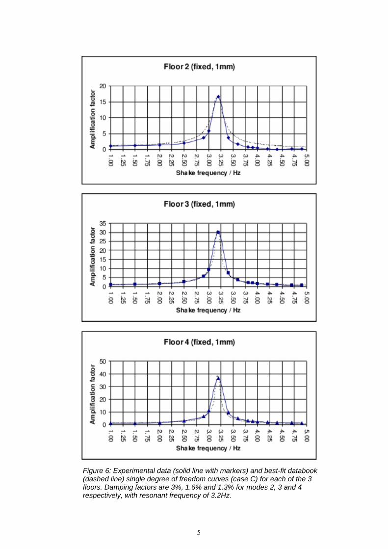
As an example, in Figure 6 the Fourier Transforms obtained from the structure were used to construct a response plot. In this case, the structure was fixed rigidly to the base of the shaking table with no soil present. The x-axis of these plots is the shaking frequency of each test, while the y-axis is the amplification factor. This is the Fourier transform amplitude, at the shaking frequency of the floor in question, divided by that of the base.

5

Figure 6: Experimental data (solid line with markers) and best-fit databook (dashed line) single degree of freedom curves (case C) for each of the 3 floors. Damping factors are 3%, 1.6% and 1.3% for modes 2, 3 and 4 respectively, with resonant frequency of 3.2Hz.

6

Operation of Equipment

Shaking table

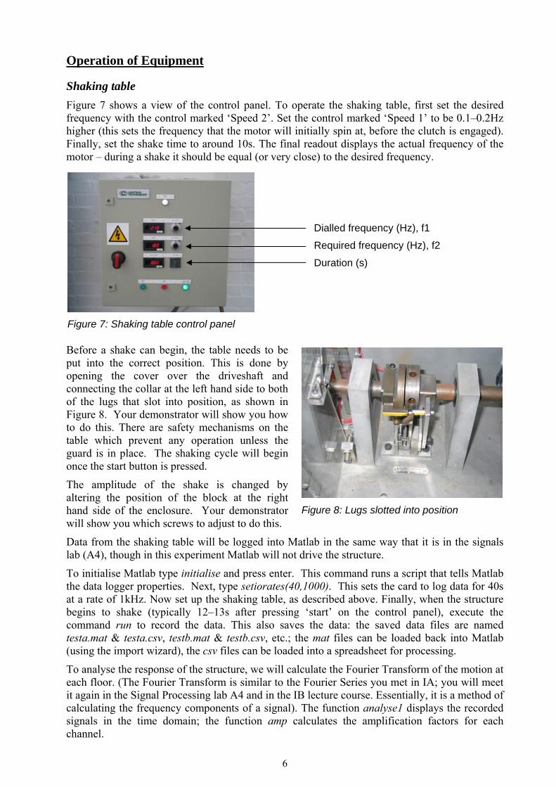
Figure 7 shows a view of the control panel. To operate the shaking table, first set the desired frequency with the control marked ‘Speed 2’. Set the control marked ‘Speed 1’ to be 0.1–0.2Hz higher (this sets the frequency that the motor will initially spin at, before the clutch is engaged). Finally, set the shake time to around 10s. The final readout displays the actual frequency of the motor – during a shake it should be equal (or very close) to the desired frequency.

Before a shake can begin, the table needs to be put into the correct position. This is done by opening the cover over the driveshaft and connecting the collar at the left hand side to both of the lugs that slot into position, as shown in Figure 8. Your demonstrator will show you how to do this. There are safety mechanisms on the table which prevent any operation unless the guard is in place. The shaking cycle will begin once the start button is pressed.

The amplitude of the shake is changed by altering the position of the block at the right hand side of the enclosure. Your demonstrator will show you which screws to adjust to do this.

Data from the shaking table will be logged into Matlab in the same way that it is in the signals lab (A4), though in this experiment Matlab will not drive the structure.

To initialise Matlab type initialise and press enter. This command runs a script that tells Matlab the data logger properties. Next, type setiorates(40,1000). This sets the card to log data for 40s at a rate of 1kHz. Now set up the shaking table, as described above. Finally, when the structure begins to shake (typically 12–13s after pressing ‘start’ on the control panel), execute the command run to record the data. This also saves the data: the saved data files are named testa.mat & testa.csv, testb.mat & testb.csv, etc.; the mat files can be loaded back into Matlab (using the import wizard), the csv files can be loaded into a spreadsheet for processing.

To analyse the response of the structure, we will calculate the Fourier Transform of the motion at each floor. (The Fourier Transform is similar to the Fourier Series you met in IA; you will meet it again in the Signal Processing lab A4 and in the IB lecture course. Essentially, it is a method of calculating the frequency components of a signal). The function analyse1 displays the recorded signals in the time domain; the function amp calculates the amplification factors for each channel.

Figure 7: Shaking table control panel

Required frequency (Hz), f2

Dialled frequency (Hz), f1

Required frequency (Hz), f2

Duration (s)

Duration (s)

Figure 8: Lugs slotted into position

7

Oedometer

An oedometer sample is contained within a metal cylinder 19.2mm deep, and squeezed between 2 porous discs 75mm in diameter. These allow water to escape from a wet sample as the load is increased, though with the dry samples here this feature is superfluous. To prepare the sample, hold the steel ring on top of the bottom disc and pour sand in at a constant rate. A loose sample is achieved by pouring sand fairly quickly from a very low height (a few mm above the base), while a dense sample needs a slow pour from a height of 30 or 40cm. Your demonstrator will give you some advice on how best to pour to achieve your target density. The sample is then fastened into the carrier. Each group will carry out a test at one of the following relative densities: 40%, 50%, 60% or 80%.

As this is a dry sand sample, there is no need to wait for more than a couple of seconds for the reading to stabilise (a wet clay sample might take several days to fully consolidate when loaded). Compression is measured by an LVDT. This gives a voltage output in the range ±4V over a 10mm displacement range. The calibration constant (in V/mm) is required to calculate the total displacement – this will be provided in the lab session.

Calibration constant = ....................................................... V/mm

Results

Oedometer test

Calculation of sample properties

The voids ratio is defined as the ratio of the volume of voids to the volume of solid grains.

Total volume of sample = 53232 108.4821019.2)10(7544

=π

=hdπ

m3

Mass of empty sample carrier = .....................kg

Mass of full sample carrier = ..........................kg

Total mass of sand = .......................................kg

The specific gravity of the sand used is 2.65 (i.e. its solid grains are 2.65 times more dense than water). The total sand volume is therefore the sand mass divided by 2650.

Sample sand volume = ....................................m3

Volume of air in the sample = (total sample volume) – (sample sand volume)

Air volume = ...................................................m3

Voids ratio = Air volume / Sand volume = ...............................

Relative density is calculated by:

minmax

max

ee

ee=I

sampleD

ID for prepared sample = ..................................

For the sand used, emax = 1.014 and emin = 0.613

N.B. See Website for more information

8

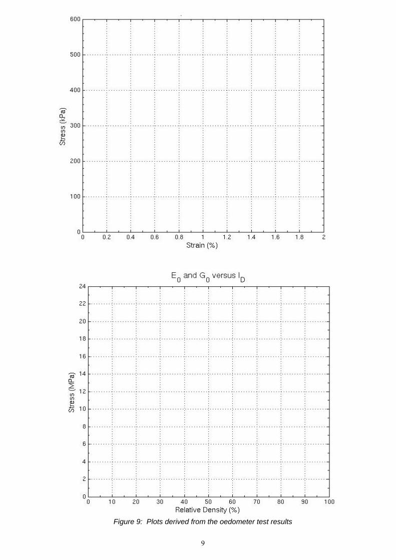
Record your results in the table below. There are 3 additional strain columns for you to record results from the other groups. When you have a full set of results, plot them on the 2 grids provided. Calculate the stiffness and shear modulus of the model sand bed, which has a relative density of 90%. The stiffness is simply the gradient of the loading line. The shear modulus is calculated using equation 2 (p.4).

0 1 3 5

10

15

20

15

10

5 3 1 0

Load (kg)

Sam

ple Pressure

(kPa) =

Load x 24.8

LVD

T output

(V)

Displacem

ent (m

m) =

LVD

T

output /calibration constant

Change in

displacement

from 0kP

a (m

m)

Strain

(displacement

change / 19.2)

ID =

Strain

ID =

Strain

ID =

Strain

ID =

9

Figure 9: Plots derived from the oedometer test results

10

The shear modulus G can be used to give the soil spring stiffness, K. This can then be used to refine the theoretical model of the system by incorporating a fourth degree of freedom. Calculate K for each of the 3 samples using the equation:

0.273.73

)(2

2.4

+b

l

ν

Gb=K

3

Summary of results:

Relative density ( %)

Stiffness, E

(MPa) Shear modulus, G

(MPa) Soil spring stiffness, K

(kNm-1)

90% (model sand bed)

Shaking table test results

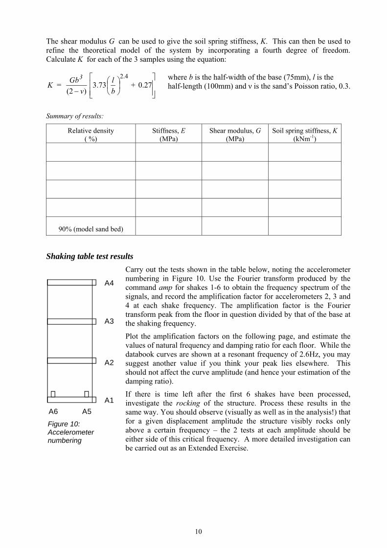
Carry out the tests shown in the table below, noting the accelerometer numbering in Figure 10. Use the Fourier transform produced by the command amp for shakes 1-6 to obtain the frequency spectrum of the signals, and record the amplification factor for accelerometers 2, 3 and 4 at each shake frequency. The amplification factor is the Fourier transform peak from the floor in question divided by that of the base at the shaking frequency.

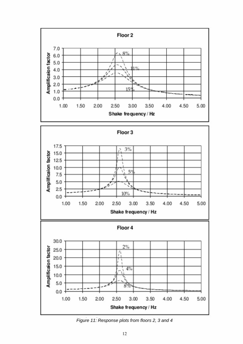
Plot the amplification factors on the following page, and estimate the values of natural frequency and damping ratio for each floor. While the databook curves are shown at a resonant frequency of 2.6Hz, you may suggest another value if you think your peak lies elsewhere. This should not affect the curve amplitude (and hence your estimation of the damping ratio).

If there is time left after the first 6 shakes have been processed, investigate the rocking of the structure. Process these results in the same way. You should observe (visually as well as in the analysis!) that for a given displacement amplitude the structure visibly rocks only above a certain frequency – the 2 tests at each amplitude should be either side of this critical frequency. A more detailed investigation can be carried out as an Extended Exercise.

A4

A3

A2

A1

A5A6

Figure 10: Accelerometer numbering

where b is the half-width of the base (75mm), l is the half-length (100mm) and ν is the sand’s Poisson ratio, 0.3.

11

Results tables for shaker

Shake number

Frequency/Hz Shake amplitude/mm

Accelerometers measured

File name

1 1.5 1 A1, A2, A3, A4

2 2.2 1 A1, A2, A3, A4

3 2.5 1 A1, A2, A3, A4

4 2.8 1 A1, A2, A3, A4

5 3.2 1 A1, A2, A3, A4

6 4.0 1 A1, A2, A3, A4

Now process these results. If there is time, continue with tests 7-10.

7 1.5 1 A1, A4, A5, A6

8 2.8 1 A1, A4, A5, A6

9 1.5 3.5 A1, A4, A5, A6

10 2.2 3.5 A1, A4, A5, A6

Shake number

Freq/Hz Shake amp/mm

A2/A1 A3/A1 A4/A1 A5/A1 A6/A1

1 1.5 1 xxxxxx xxxxxxx

2 2.2 1 xxxxxx xxxxxxx

3 2.5 1 xxxxxx xxxxxxx

4 2.8 1 xxxxxx xxxxxxx

5 3.2 1 xxxxxx xxxxxxx

6 4.0 1 xxxxxx xxxxxxx

7 1.5 1 xxxxxxx xxxxxx

8 2.8 1 xxxxxxx xxxxxx

9 1.5 3.5 xxxxxxx xxxxxx

10 2.2 3.5 xxxxxxx xxxxxx

12

Figure 11: Response plots from floors 2, 3 and 4

13

Best fit data from graphs

Floor Frequency of maximum amplification factor (Hz)

Damping ratio

Floor 2

Floor 3

Floor 4

Compare your values of frequency and damping ratio with the theoretical and experimental values from Figure 6 (another 4-degree of freedom system, though this time without soil). The IA experiment was a 3-degree of freedom system, and so direct comparison is not possible.

Conclusions

Soil stiffness is non-linear, but can be measured in an oedometer.

The response and natural frequencies of the structure change when it is placed on realistic (non-fixed) foundations:

Comment on the change in damping:

Comment on the change in natural frequency:

Rocking frequency:

At low frequency/amplitude there is little or no rocking

At higher frequency/amplitude rocking frequency = shaking frequency

There is a threshold frequency above which amplification factors are significantly higher

Transient loading due to earthquakes can result in unusual modes of vibration

_____________________________________________________________________________________

APPENDIX: Summary of Matlab code

initialise Creates software representation data acquisition card. Only needs to be run once. setiorates(40,1000) Sets Matlab to record data for 40s at a rate of 1kHz. run Starts logging data. Run this command when the structure first shakes. analyse1 Displays the captured data in the time domain. amp(freq) Calculates the Fourier transform and amplification factor for each floor. The freq argument is optional – if not given, the function will calculate the

shaking frequency from the data (overridden if the argument is given a value). Filter Filters data to reduce noise – use this for data from accelerometers A5 and A6 (for rocking analysis). Note Filter not filter.