SOIL MOISTURE EXPERIMENTS IN 2002

(SMEX02)

Experiment Plan

June 2002

TABLE OF CONTENTS 0 Executive Summary 4 1 Overview and Scientific Objectives 5

1.1 Soil Moisture Mission (EX-4a) 6 1.2 Global Water and Energy Cycle (GWEC) 7 1.3 Advanced Microwave Scanning Radiometer (AMSR) 8 1.4 Soil Moisture Experiments in 2002 (SMEX02) 8

2 SMACEX-Soil Moisture Atmosphere Coupling EXperiment 10 2.1 Background 10 2.2 Scientific Approach and Expected Results 12

3 Satellite Observing Systems 19 3.1 Aqua Advanced Microwave Scanning Radiometer (AMSR-E) 19 3.2 Special Sensor Microwave Imager (SSMI) 20 3.3 European Radar Satellite (ERS-2) 20 3.4 Envisat Advanced Synthetic Aperture Radar (ASAR) 21 3.5 Radarsat 22 3.6 Terra Sensors 22 3.7 Landsat Thematic Mapper 23 3.8 Advanced Very High Resolution Radiometer (AVHRR) 25 3.9 Geostationary Operational Environmental Satellites (GOES) 25 3.10 SeaWinds Quickscat 26

4 Aircraft Remote Sensing Instruments 27 4.1 Polarimetric Scanning Radiometer (PSR) 27 4.2 Passive and Active L and S Microwave Instrument (PALS) 30 4.3 Electronically Scanned Thinned Aperture Radiometer (ESTAR) 31 4.4 Airborne Synthetic Aperture Radar (AIRSAR) 33 4.5 Global Positioning System (GPS) Technique 33 4.6 Utah State University Visible and Infrared Sensors 35

5 Remote Sensing Aircraft Mission Design 36 5.1 NCAR C-130 36 5.2 NASA P-3B 37 5.3 NASA DC-8 38 5.4 Canadian Twin Otter 42 5.5 Utah State University Piper 43

6 Iowa Study Region 47 6.1 Watershed Sites 49 6.2 Regional Sites 53

7 Schedule 55 8 Ground Data Collection 56

8.1 Tower Based Surface Flux Measurements 56 8.2 Lidar/Sodar/Radiosondes 57 8.3 Sun Photometer 57 8.4 Vegetation and Land Cover 57 8.5 Soil Moisture 58

2

8.6 Soil and Surface Temperature 60 8.7 Soil Surface Roughness 61 8.8 Ground Based Microwave Radiometer 62

9 Regional Meteorological and Climate Networks 63 9.1 Soil Climate Analysis Network (SCAN) 64 9.2 NSTL Meteorological Stations 65 9.3 Iowa Environmental Mesonet 66

10 SMEX02/SMACEX Tower Flux Measurements 67 10.1 Eddy Covariance Measurements 67 10.2 Ancillary Measurements 69 10.3 Intercomparison 70 10.4 Instrument Height/Depth and Position 70 10.5 Selected Test Sites 72

11 Protocols for Ground Sampling 74 11.1 General Guidelines for Field Sampling 74 11.2 Watershed Site Surface Soil Moisture and Temperature 74 11.3 Regional Site Surface Soil Moisture and Temperature 77 11.4 Theta Probe Soil Moisture Sampling and Processing 80 11.5 Gravimetric Soil Moisture Sampling with the Scoop Tool 85 11.6 Gravimetric Soil Moisture and Bulk Density Sampling with the Coring Tool 86 11.7 Gravimetric Soil Moisture Sample Processing 88 11.8 Watershed Site Bulk Density and Surface Roughness 90 11.9 Hydra Probe Soil Moisture and Apogee Surface Temperature Installations 94 11.10 Watershed Site Vegetation Sampling 96 11.11 Plant Canopy Analyzer Measurements 100 11.12 Global Positioning System (GPS) Coordinates 102

12 References 107 13 Investigator Abstracts 113 14 Contact List 182 15 Logistics 185

15.1 Security 185 15.2 Safety 185 15.3 Hotels 188 15.4 Shipping Information 189 15.5 Directions 190 15.6 Local Contacts 192

3

0 EXECUTIVE SUMMARY Soil moisture field experiments have been very successful at addressing a broad range of science question, focusing technology development and demonstration, and providing educational experiences for undergraduate and graduate students. The data have been used in studies that went well beyond the algorithm research, primarily due to an emphasis on developing map-based products. For 2002, a soil moisture field experiment (SMEX02) is proposed that would support the science needs of the NASA Land Surface Hydrology Program Soil Moisture Mission (EX-4a), the NASA Global Water and Energy Cycle Research Program, the EOS Aqua Advanced Microwave Scanning Radiometer, and NOAA-DOD prototype land parameter algorithms utilizing data from the Special Sensor Microwave Imager (SSM/I). The objectives of SMEX02 are to understand land-atmosphere interactions, extension of instrument observations and algorithms to a broader range of vegetation conditions, validation of land surface parameters retrieved from SSM/I and potentially AMSR data, and the evaluation of new instrument technologies for soil moisture remote sensing. We have chosen to address the combined objectives with ground/aircraft/spacecraft observations over sites in Iowa during the summer of 2002. This report describes the elements of SMEX02 in detail. Coverage includes the aircraft and satellite soil moisture sensors, the land atmosphere experiments, aircraft missions, ground data collection, regional networks and test sites. A set of abstracts describing the research goals of the individual investigators is also included.

4

1 OVERVIEW AND SCIENTIFIC OBJECTIVES The significance of a hydrologic state variable is expressed well in the recent description of NASA’s Global Water and Energy Cycle research program. Water is at the heart of both the causes and the effects of climate change. Ascertaining the rate of cycling of water in the Earth system, and detecting possible changes, is a first-order problem with regard to the renewal of water resources and hydrologic hazards. A more complete understanding of water fluxes, storage, and transformations in the land, atmosphere, and oceans will be the central challenge to the hydrological sciences in the 21st century. Improved knowledge and prediction of the water cycle can yield large benefits for resource management and regional economies if variability and uncertainties can be understood, quantified and communicated effectively to decision-makers and to the public. The overarching objective is to improve the understanding of the global water cycle to the point where useful predictions of regional hydrologic regimes can be made. This predictive capability is essential for practical applications to water resource management and for validating scientific advances through the test of real-life prediction. Soil moisture is the key state variable in hydrology: it is the switch that controls the proportion of rainfall that percolates, runs off, or evaporates from the land. It is the life-giving substance for vegetation. Soil moisture integrates precipitation and evaporation over periods of days to weeks and introduces a significant element of memory in the atmosphere/land system. There is strong climatological and modeling evidence that the fast recycling of water through evapotranspiration and precipitation is the primary factor in the persistence of dry or wet anomalies over large continental regions during summer. As a result, soil moisture is the most significant boundary condition that controls summer precipitation over the central U.S. and other large mid-latitude continental regions, and essential initial information for seasonal predictions. A common goal of a wide range of agencies and scientists is the development of a global soil moisture observing system (Leese et al. 2001). Providing a global soil moisture product for research and application remains a significant challenge. Precise insitu measurements of soil moisture are sparse and each value is only representative of a small area. Remote sensing, if achievable with sufficient accuracy and reliability, would provide truly meaningful wide-area soil wetness or soil moisture data for hydrological studies over large continental regions. Development and implementation of the remote sensing component of a global soil moisture observing system will require advancements in science and technology. Many aspects of the research require validation and demonstration, which can only be accomplished through controlled large-scale field experimentation. Large-scale field experimentation requires significant resources to be successful that are usually contributed from several programs. Through a series of workshops and research announcements science and technology priorities for soil moisture remote sensing have been identified. Elements requiring field experimentation were identified and, to the extent possible, combined into Soil Moisture Experiments for 2002 (SMEX02). This model has worked well in soil moisture research in the past and will be applied in 2002. SMEX02 will focus on microwave remote sensing of soil moisture in an agricultural setting. Issues not addressed in this experiment will be the focus of future field experiments.

5

At the present time there are three programs that significantly influence the direction of research and the requirements of a soil moisture field experiment. These are the Soil Moisture Mission (EX-4a), Global Water & Energy Cycle (GWEC) Research and Analysis, the Advanced Microwave Scanning Radiometers (AMSR) on Aqua and ADEOS-II. The relevant science needs of each program are described in the following sections. These were merged into the SMEX02 experiment plan. 1.1 Soil Moisture Mission EX-4a Soil moisture is recognized by the NASA Post 2002 program as a critical measurement As a result, several scientific reviews were conducted to define a Soil Moisture Mission. The final report can be found at http://maximus.ce.washington.edu/~tempcm/Post2002/smm3.html. This mission is based on a scientific consensus that an L band microwave remote sensing with high spatial resolution (<10 km) is needed for soil moisture. Technology development will be needed before such a mission can be implemented. Many of the science issues related to this mission can be addressed immediately. These include: • Conduct a field experiment to collect passive microwave data to extend the calibration and

validation to agricultural crops at peak biomass. • Conduct a field experiment to collect passive microwave data to validate algorithm

performance in regions with diverse topography. • Conduct field experiments to collect passive microwave data to explore their usefulness in

different types of forest canopies. • Soil moisture retrieval algorithms that rely on ancillary data or multichannel data need to be

compared • Evaluations of soil moisture retrieval techniques with C band data can be performed using

near future satellite missions such as EOS-PM and ADEOS-II. Conduct field experiments to collect aircraft and ground passive microwave data concurrent with AMSR over passes that will allow the validation of algorithms and definition of the scaling behavior of the measurements.

• Establish a series of validation sites where high quality ground data will be collected consistently.

• Airborne simulators for each proposed space instrument need to be built for pre-mission studies and mission-current validation flights.

As part of this research we must also consider the contributions it can make to the ESA Soil Moisture Ocean Salinity (SMOS) mission and how EX-4a can in turn benefit. SMOS is a passive microwave L band soil moisture measurement mission with a 50-km spatial resolution. Although it will not have the desired EX-4a spatial resolution, such a mission would provide a first experience and a valuable science data product. At the present time, the launch is anticipated in 2006 (http://www-sv.cict.fr/cesbio/smos/). SMOS will utilize two dimensional synthetic aperture radiometry and will employ a variation on soil moisture algorithms that has

6

not been rigorously calibrated and validated. The instruments utilized and field experiments conducted in SMEX02 are highly relevant to the SMOS project. 1.2 Global Water & Energy Cycle (GWEC) The most recent NASA initiative relevant to soil moisture research is the Global Water & Energy Cycle (GWEC) program. A current focus of this program is to explore the connection between weather-related fast dynamical/physical processes that govern energy and water fluxes, and climate responses and feedbacks. The objective of this research is to address the water and atmospheric energy cycles as a single integrated problem. This approach includes exploring the response of regional hydrologic regimes (precipitation, evaporation, and surface run-off) to changes in atmospheric general circulation and climate, and the influence of surface hydrology (soil moisture, snow accumulation and soil freezing/thawing) on climate. Key scientific questions of this program are listed below along with specific issues that can be addressed by SMEX02. Is the global cycling of water through the atmosphere accelerating? • Assessment of large-scale variability patterns and/or global trends in the occurrence of

extreme hydrologic events (e.g., floods and droughts), based on the analysis of global remote sensing and insitu observational data.

• Estimation of evaporation fluxes over the land and oceans, based on the assimilation of relevant observational data, and advanced parameterizations of model sub-grid scale processes (e. g. planetary boundary layer dynamics).

• Diagnostics of spatial and temporal changes in the distribution of surface energy and water storage; diagnostics of atmospheric responses to changes in ocean and land boundary conditions.

What are the effects of clouds and surface hydrologic processes on climate change? • Use satellite remote sensing to improve land surface process modeling and the understanding

of soil-vegetation-atmosphere interactions at regional or greater scales. • Establish the interrelationships and feedbacks among clouds, precipitation, boundary layer,

and land surface processes using improved coupled land-atmosphere models and assimilated data.

• Determine how land-atmosphere interactions, as affected by orography, vegetation, and soil, affect the predictability of large-scale terrestrial hydrology and atmospheric systems, including precipitation and runoff.

How are variations in local weather, precipitation, and water resources related to global climate change? • Analysis of the effect of spring and early summer hydrologic anomalies (snow accumulation,

soil moisture, soil freezing and thawing) on subsequent weather and precipitation patterns, and hydrologic phenomena (impacts on runoff, water storage, and inland water bodies), and how climate change might affect such anomalies in the future.

• Establish the scientific justification for future space-based observations of soil moisture, snow, surface water, or other hydrologic variables, through scientific analysis and field

7

investigations, including the improvement in our understanding of the global water and energy cycle, floods and droughts, and climate change.

• Determine techniques for transferring regional (e.g. GAPP) hydrologic process understanding and prediction tools to other areas of the world, using remotely sensed and emerging Coordinated Enhanced Observing Period (CEOP) observations scheduled for 2001 to 2003.

1.3 Advanced Microwave Scanning Radiometer (AMSR) While it will be years before a spaceborne L band instrument will be available, a major opportunity exits to maximize the AMSR instruments that are part of the recently launched Aqua satellite and ADEOS-II (2002-2003). A critical element of the AMSR program is validation of the soil moisture products. In addition, there are gaps in the knowledge base available for algorithm development, especially over vegetation. The EOS Aqua AMSR-E science team is highly involved in the SMEX02 program. AMSR includes C band channels that offer improved capabilities for soil moisture sensing over current satellite options (even though it is less optimal than the proposed L band radiometers proposed for SMOS and EX-4a). The spatial resolution will be significantly better than its predecessor SMMR. All AMSR research will contribute to efforts to understand and validate soil moisture retrievals from EX-4a and SMOS. Validating large footprint observations is a difficult task and in the past it has been neglected. We have to commit to collecting real soil moisture data, not surrogate variables, and these should correspond to the sensor measurement depth. What we learn in attempting this for AMSR will be of great benefit to EX-4a. 1.4 Soil Moisture Field Experiment for 2002 (SMEX02) Field experiments, in particular the series that has been conducted at the Southern Great Plains (SGP) site, have been very successful at addressing a broad range of science and instrument questions. The data have been used in studies that went well beyond the algorithm research, primarily due to an emphasis on developing map-based products. For 2002, a field experiment is proposed that would support the science needs of EX-4a, GWEC, and AMSR. Main elements of the experiment are to understand land-atmosphere interactions, validation of AMSR brightness temperature and soil moisture retrievals, extension of instrument observations and algorithms to more challenging vegetation conditions, and the evaluation of new instrument technologies for soil moisture remote sensing. We have chosen to address the combined objectives with ground/aircraft/spacecraft observations over sites in Iowa during the summer of 2002. This report describes the elements of SMEX02 in detail. Coverage includes the aircraft and satellite soil moisture sensors, the boundary layer experiments, aircraft missions, ground data

8

collection, regional networks and test sites. A set of abstracts describing the research goals of the individual investigators is also included.

9

2 SMACEX-Soil Moisture Atmosphere Coupling EXperiment A number of field experiments in the past, including SGP97 and SGP99, have been designed to investigate land surface-atmosphere coupling and the role of remote sensing in Land Atmosphere Transfer Schemes (LATS). However, in these studies, methodologies for upscaling and aggregation have not been adequately developed, implemented and tested because the necessary measurements, models and other tools to perform these tasks either have not existed and/or have not merged in the necessary way. Moreover data quality depends to a degree on the conditions encountered in a particular experiment. Hence building a diverse knowledge base needed to understand the complex interaction of the land surface and atmosphere requires a continued effort in collecting the necessary field observations over different land cover types and climatic conditions. An integral part of SMEX02 is an experiment designed to address these concerns. The SMACEX project is designed to collect atmospheric and remote sensing data over a range of spatial and temporal scales necessary to investigate local and regional scale impacts of landscape heterogeneity on water and energy exchanges. 2.1 Background SMACEX will address several timely research foci in the area of water and energy cycling across the land-atmosphere interface (see below). With additional support for flying time and data processing, the Twin-Otter can collect surface-layer and atmospheric boundary-layer (ABL) flux data. Support for two other remote sensing activities, namely aircraft-based high resolution optical remote sensing data and ground-based Lidar observations of wind and water vapor concentrations in the ABL, will provide simultaneous landscape and atmospheric properties covering a wide range of temporal and spatial scales. Combining these observations together with a network of 15-20 tower-based flux observations will result in a complete set of distributed surface and atmospheric data, allowing for LATS and Large Eddy Simulation (LES) model validation and development and testing of methodologies to bridge the scales from local to regional. A schematic diagram summarizing the measurement and modeling activities (experimental logistics) proposed for the project and the overall framework addressing up-scaling issues is given in Figure 1. This figure also illustrates the interdependency of the proposed activities and that all components of the project are required in order to achieve proposal goals and objectives. The expected advances with the coupled measurement and modeling program will address one of NASA’s core missions of seeking to rigorously bridge between remotely sensed data and operational forecast models, including advances in operational data assimilation schemes. The overall objective of this work is to use a direct-measurement/remote sensing/modeling approach to understand how horizontal heterogeneities in vegetation cover, soil moisture and other land-surface variables influence the exchange of moisture and heat with the atmosphere. The field observations will support the analysis of heterogeneities ranging from within field or patch to the regional scales that are commensurate with prediction models of weather and climate. The unique in-situ and aircraft measurements of atmospheric and soil variables and

10

fluxes to be provided in the SMACEX data set are of primary importance. They will be used both to validate fluxes diagnosed using remote sensing methods at various scales, and in evaluating results from the LES-remote sensing model that will be used to develop horizontal scaling relationships. The experimental approach is thus also an "up-scaling" endeavor, investigating how remote sensing data at different horizontal and temporal scales may be utilized for both diagnosis and prediction of the surface energy exchanges from patch to regional scales. In particular, we focus on the effects of observation and model scale on the importance and effectiveness of assimilation techniques.

Figure 1. Schematic summarizing measurement and modeling activities and their interrelationships. Validation (blue arrows) of both the high resolution (10 to 100 m) output from LATS and LES remote sensing models is performed with the flux towers and Lidar data, while up-scaling techniques (red arrows) to the coarser resolutions ( > 100 m to 10 km) validated with Lidar and aircraft fluxes. Validation of the prognostic LATS is achieved through validated up-scaled diagnostic LATS remote sensing models.

11

2.2 Scientific Approach and Expected Results

2.2.1 Large Eddy Simulation Investigations

The effects of surface heterogeneity on atmospheric turbulence and mean air properties and resulting feedbacks on the land surface fluxes can be captured in a modeling framework using LES. LES models simulate the space and time dynamics of ABL turbulence and the interactions with the land surface using a numerical solution of the Navier-Stokes equations (e.g., Albertson and Parlange, 1999). Most studies addressing land surface heterogeneity using LES have described surface boundary conditions as predefined fluxes with artificial variability (e.g. Hadfield et al., 1991, 1992; Avissar et al., 1998; Avissar and Schmidt, 1998; Cai, 1999), or with spatial variability defined to match the surface flux fields estimated from experimental data at a particular site (e.g. Hechtel et al., 1990; Eastman et al., 1998). The questions of how the surface heterogeneity affects ABL heterogeneity, and how the surface and air properties in turn affect the flux fields that develop over a region with heterogeneous surface properties are left unanswered in most LES studies.

The LES-remote sensing model recently developed by Albertson et al (2001) couples remotely sensed surface temperature and soil moisture fields (2D) to the dynamic (4D) ABL variables via a LATS model, which includes separate and explicit contributions from soil and vegetation (i.e. two sources) to mass and energy exchanges. This is a merger of active lines of research: the use of remotely-sensed land surface properties to study water and energy fluxes, and the use of LES to study the impacts of surface variability on ABL processes. This LES-remote sensing model can run over a ~10 km2 domain at relatively high spatial resolution (~100 m) with remotely sensed vegetation cover, surface soil moisture and temperature defining surface heterogeneities governing atmospheric exchanges/interactions with the land surface. Typically, LATS are either driven by a network of surface meteorological observations, or use energy conservation principles applied to ABL dynamics to deduce air temperature (Anderson et al., 1997). However, neither approach considers the resulting impact/feedback of surface heterogeneity on atmospheric turbulence and the resulting spatial features of the mean air properties, particularly at the patch or local scale. LES predictions will provide a benchmark for assessing the impact of a range of surface heterogeneity features on LATS predictions neglecting such coupling.

To validate the results of LES turbulence and flux simulations as the basis for later up-scaling parameterizations, the fields of LES-derived air properties will be compared to Lidar observations (providing multidimensional “snapshots” of the turbulent fields in the ABL), and the LES-derived spatially-distributed heat fluxes will be evaluated in the context of the network of tower–based flux measurements. The tower-based flux observations, the high-resolution optical remote sensing data, and the Lidar observations will not only provide patch-scale validation of the LES predictions, but also allow us to investigate the interactions of high-resolution surface fields with high-resolution turbulence fields. Such observations and analyses are needed to ultimately account for the subgrid processes needed to link remotely-sensed land surface fields with coarser-scale atmospheric models. The aircraft-based measurements will validate flux predictions on scales commensurate with the nominal grid size of weather

12

forecasting models (i.e., ~ 10 x 10 km (mesoscale models), to ~ 100 x 100 km (climate models scales)).

LES results and Lidar/flux observations will support a thorough investigation of spatial scaling relationships and identification of variables or combinations of variables that can be scaled to weather and climate models, providing accurate grid-averaged fluxes. In fact, some initial insight into scaling relationships between the surface and the lower atmosphere has been reported in the results from Albertson et al. (2001). It was found that the correlation between time-averaged maps of surface and air temperatures is dependent on the length scale of the heterogeneous surface features, and that the horizontal standard deviation of time-averaged air temperature decreased logarithmically with height in the atmospheric surface layer. Moreover, the mean air temperature contains spatial variability induced preferentially from variations in surface temperature occurring at scales greater than 500-1000 m. Hence, the feedback strength between the land and the atmosphere is shown to be scale-dependent for the range of length scales (i.e.

) studied here. km110≤ 2.2.2 LATS Investigations

The investigators have developed several related LATS models that have been used in a diagnostic mode, where a combination of visible, near-IR, thermal, and microwave remote sensing data are used to estimate land surface fluxes, soil moisture and other characteristics over various spatial and temporal scales. The versions of the diagnostic models are complementary, in that they use remote sensing data measured over different space and time scales and produce flux estimates over these scales. Recent work has merged model versions such that flux estimates made at larger scales (5-10 km) can be successfully "disaggregated" to the 30-m scale of remote sensing data from aircraft, Landsat and potentially other high resolution satellite (e.g., ASTER) instruments. The various LATS models that can operate at the patch scale will be validated using tower-based flux measurements, fluxes derived indirectly from Lidar and LES output, while those LATS operating at the 5-10 km scale will be compared to aircraft, and LES aggregated values. Incorporation of microwave data in combination with visible, near-infrared and thermal-infrared is considered to have great potential in constraining two-source LATS predictions. This is because the microwave-derived surface soil moisture may permit an independent determination of the soil evaporation component, critical in assessing energy partitioning between soil and vegetation components in partial canopies. The result of not directly considering feedback effects of surface heterogeneity on atmospheric turbulence and mean air properties will be deduced from the comparison of the LATS fluxes (with no local feedbacks) with the LES output, Lidar observations and flux measurements (which include feedbacks). The vegetation/land surface scheme (called the “two-source” approach) employed is the common thread among the various LATS versions and related remote sensing parameterizations employed in this project. This two-source scheme, where the two sources refer to fluxes originating from the individual soil and vegetation sub-components, is essential for interpreting the relationships between aerodynamic and radiometric temperature as a function of vegetation cover and viewing angle of the remotely-sensed infrared brightness temperatures (Norman et al, 1995, Kustas et al., 13

2000). This two-source-remote sensing modeling framework is considered a major advancement over single-layer schemes (e.g., Hall et al., 1992; Vining and Blad, 1992), which do not consider the individual soil and vegetation contributions to the total or composite heat fluxes and soil and vegetation temperatures to the radiometric temperature measurements (Norman et al., 1995). In areas of partial vegetation cover the remotely sensed surface temperature is a mixture of vegetation and soil temperatures. As the soil dries these temperatures can differ greatly. Biophysical processes related to the coupling of water and carbon cycles through plants depend on the foliage temperature while the soil processes, such as decomposition and respiration, depend on the soil temperature. The work proposed in this project will expand the impact of the remote sensing data as the combination of the two-source model with microwave and infrared data enable the partitioning of the surface temperature into the vegetation and soil components, as needed to accurately assess the water and carbon cycling in vegetation and soils. At the larger scales, an Atmospheric-Land-EXchange-Inverse model (ALEXI, Anderson et al., 1997; Mecikalski et al., 1999) has been developed to diagnose surface latent and sensible heat fluxes at regional scales at a resolution of 5 to 10 km. A strength of this model is that it uses time-differencing (made approximately 4 hours apart) of radiometric temperatures from GOES satellites as input rather than single-time measurements. Such differencing has been shown to be less sensitive than single-time measurements to the effects of view angle (Diak, 1990), emissivity and atmospheric corrections (Anderson et al., 1997). A second important feature is that energy closure is achieved using an Atmospheric Boundary Layer (ABL) closure scheme and ABL temperature profiles that can be obtained from radiosonde data, or even from a forecast model. This avoids the use of screen-level atmospheric measurements, which suffer from errors of representativeness (made at about 100-km intervals and at potentially unrepresentative sites) and also are made too close to the surface, so that errors from any surface source will produce large errors in the estimated fluxes. Using the ABL closure, ALEXI derives local estimates of air temperature at an interface height of about 50m. As part of complementary NASA and NOAA funding, an ALEXI version based in the mathematics of statistical interpolation (SI-ALEXI) has been put into a real-time mode and linked with the CIMSS mesoscale forecast model. Because the predictive version of ALEXI (ALEX) is used as its land-surface component, the CIMSS model has a built-in compatibility with ALEXI. The SI enhancement enables multiple signals of the surface water/energy balance, to be incorporated into ALEXI. Such inputs include low-level measurements of air temperature and humidity (e.g., Mahfouf, 1991; Yang et al., 1994; Mecikalski et al., 1997), radiometric temperatures (Mecikalski et al., 1999), as well as microwave estimates of near-surface soil moisture (Kustas et al., 1998). A relatively simple dual-temperature difference (DTD) approach for using time rate of change in radiometric and air temperature observations to compute the surface heat fluxes was recently derived and evaluated using data from several different field sites covering a wide range of environmental conditions (Norman et al., 2000a). Similar to ALEXI, the approach reduces the effect of errors associated with radiometer calibration, emissivity variations and use of non-local air temperature and wind speed data. Comparisons with heat fluxes predicted by ALEXI indicates that the DTD method has potential for regional scale applications using satellite data and a synoptic weather station network. It is also computationally very efficient taking 1/30 the computational time of ALEXI (Kustas et al., 2000).

14

A drawback of ALEXI and DTD approaches, however, is that the source of thermal-IR data (GOES) and the atmospheric boundary layer closure dictate the larger resolution of 5 to 10 km, and for many applications, including examining scaling issues, we need to estimate fluxes at much finer spatial scales. Additionally, temporal changes of infrared temperatures are only available from GOES satellites at a maximum resolution of ~5 km, but not from satellites with higher spatial resolution. The framework of the two-source model outlined by Norman et al (1995) will be the bridge between ALEXI and the high-resolution vegetation and thermal remote sensing data available from such satellite platforms as Landsat, ASTER, AVHRR and MODIS. The original version of this model applied to remotely sensed imagery incorporated remotely-sensed single-time radiometric temperatures (Schmugge et al., 1998), while Kustas et al. (1998; 1999a) have recently modified the two-source model to utilize microwave-derived surface soil moisture amounts to estimate the local energy balance on the 100-m scale. In these schemes, however local atmospheric measurements of air temperature were available and assumed uniform over the domain. Generally this is not an appropriate assumption for remote sensing data taken over regional spatial scales at any resolution and can lead to significant errors depending on the reference height adopted (Kustas et al., 1999b). A solution to this problem was introduced by Norman et al. (2000b), who developed a scheme for "disaggregating" ALEXI 5-km flux estimates (called DisALEXI) to the 30-m scale using high-resolution remotely sensed vegetation and thermal-infrared data, and the local 50-m air temperature estimate provided by ALEXI as the important atmospheric boundary condition in temperature. Although, this scheme makes use of energy conservation principles applied to ABL dynamics to deduce air temperature via ALEXI, it still does not consider the resulting impact/feedback of surface heterogeneity on atmospheric turbulence and the resulting spatial features of the mean air properties at the local or patch scale. The impact of these effects will be captured in a modeling framework with the adoption of the LES-remote sensing model. The diagnostic techniques embodied in these schemes (e.g., ALEXI, DTD, DisALEXI) can be adapted to provide hourly fluxes throughout the day based on clear sky observations, whether the remaining day is clear or not (Anderson et al., 1997). 2.2.3 Prognostic Modeling The role of the CIMSS forecast model in this proposed work is to evaluate the potential of remotely-sensed data and up-scaling procedures for these data in a forecasting environment. The CIMSS forecast model is run in near real-time twice daily (the model initialization times being the synoptic times of 00 and 12 UTC and for forecast durations of 48 hours) in support of regional agricultural applications (Diak et al., 1998; Anderson et al., 2000). Various applications entail model runs at resolutions of 50 km (with 46 vertical levels) for most of North America and 15 km for the upper Midwest region and northern Mexico. Other versions of the model have been used to examine surface and boundary layer parameterizations (Diak et al., 1987), for observing system simulation experiments involving satellite sounding instruments and other satellite data experiments (Diak, 1987; Diak et al., 1992; Diak et al., 1994; Wu et al., 1994; Wu

15

and Smith, 1992; Burns et al., 1997; Bayler et al., 2000) and to investigate various other physical parameterizations and numerical techniques (Raymond, 1988; Raymond, 1993; Raymond, 1994). The prognostic component of the LATS within the CIMSS model (the prognostic version of ALEXI, termed ALEX) uses a powerful and versatile parameterization for the photosynthetic process that is based on principles of light-use efficiency (LUE; Anderson et al., 2000). LUE is defined as the ratio of net CO2 assimilation to absorbed photosynthetically-active radiation ((APAR); Monteith 1977; Norman and Arkebauer 1991). In ALEX, LUE replaces the large number of vegetation-dependent parameters required by many other models (e.g., SiB2; Sellers et al. 1996). It allows an analytical solution for canopy resistance, including the effect of vapor pressure deficit, significantly improving computational efficiency and reducing input data requirements, without sacrificing generality. Since this LUE formulation deals with vegetation variables scaled to the canopy level, it is also amenable to the input of remote sensing data, inherently single-level information. Development and testing of the LUE parameterization is progressing under existing NASA and NOAA support and will leverage the efforts in this proposal. Prognostic CIMSS model runs will be made at resolutions ranging between 10 and 100 km (a typical range going from mesoscale model to climate model resolution) to evaluate the influence of remote sensing data and up-scaling procedures. Fine-scale LES flux outputs will be used to evaluate areal-averaged fluxes from the 10-km mesoscale model, and 10-km mesoscale model outputs will be averaged to the coarser resolutions for similar evaluations of the those outputs. The ALEXI (flux diagnosis model) and complementary flux disaggregation tools will be used to validate fluxes produced by the CIMSS and LES models at all scales. Flux station data from the field program, as well as other ground-based measurements (air temperature, moisture, etc.) will also be used to validate the various forecasts. To isolate the effects of land-surface variables on forecast quality (reduce potential errors from other model physical parameterizations), high-resolution measured surface solar and longwave radiation streams (both from GOES satellite data: Diak et al. 1996; Diak et al. 2000) will be used as boundary conditions (forcing) for model integrations.

2.2.4 Scaling Investigations

Fluxes are non-linearly related to most LATS input variables so that using variables defined at scales significantly larger than the patch-scale can introduce large errors in landscape-scale and regional-scale flux calculations. The effects of surface heterogeneity on LATS predictions and methods for representing subgrid scale heterogeneity are reviewed in detail by Giorgi and Avissar (1997). While much of the findings are from model simulations, a review of observational results from large scale field experiments suggests that relatively simple aggregation procedures can be used in areas where heterogeneity is not “organized”; “organized” heterogeneity is loosely defined as a region containing a patchwork of homogeneous land types > 101 km (Giorgi and Avissar, 1997). However, the observational data typically do not contain all the necessary information at the different scales to make any definitive conclusions as to the factors/processes which permit such simple aggregation procedures to be applied without resulting in large errors. Instead the development of aggregation/up-scaling procedures that

16

preserve energy conservation principles and are mathematically rigorous in scaling-up model parameters and variables have been applied to artificial surfaces to assess up-scaling errors (see Hu et al., 1999 for a review). The experimental design being proposed will allow for a more thorough investigation into the effects of subgrid/subpixel variability on LATs predictions and lead to a more fundamental understanding of the relationships between scale of heterogeneity and the relative impact on LATS predictions using aggregated input. The study area and surrounding region is primarily row crops (corn and soybean) distributed in a patchwork pattern with fields > 1 hectare in size. Thus the main length scale of heterogeneity is well defined by the field dimensions. With 20 tower flux stations, a high density of flux tower measurements will permit adequate coverage of the variation in energy fluxes across the watershed and additionally be representative of the region. The Lidar observations of atmospheric profiles will permit evaluating the effects of field scale heterogeneity in roughness, fractional cover and energy flux partitioning on atmospheric dynamics of the surface layer. The aircraft flux observations will assist in the evaluation of aggregated flux estimation from LATS using input data at different pixel resolutions. The high resolution remote sensing data will permit separating soil and vegetation components, thus allowing for evaluating the effects of up-scaling important LATS inputs, such as fractional vegetation cover, on LATS-derived fluxes. Although the microwave data will be at much coarser resolution, the combination of these data with the optical will allow for additional constraints to be imposed on LATS and LES model predictions by providing a means of estimating the soil evaporation component. Besides the variation in energy fluxes due to soil moisture/soil texture differences, the phenological differences between the two main agricultural crops and differences in management practices (i.e., conventional till, no till and ridge till) can result in significant variations in the land-surface energy exchanges across the watershed. Due to partial canopy coverage and varying crops and tillage practices, the interpretation of remotely-sensed data (including thermal data and vegetation indices) and subsequent estimation of soil and vegetation energy exchanges will be challenging (Norman et al., 1995). The magnitude of these variations are currently being assessed with energy balance measurements that have been made over several growing seasons at six locations over the watershed with varying crop (corn and soybean) and tillage history. Both the nitrogen treatment and soil type are found to significantly influence water use and hence the surface energy fluxes; differences in cumulative water use varied by as much as 400 mm by the end of the growing season. Net carbon exchanges have been monitored since 1998 over both corn and soybean. In 2000 these measurements were expanded to include CO2 fluxes over two different nitrogen management regimes in corn and included a soil respiration component for the purpose of being able to relate the soil component as a source for canopy uptake. These measurements cover the entire growing season in all years. Until 2000 the CO2 flux was estimated using Bowen ratio systems and in 2000 the LI-7500 has been added for one site. For the soil component, respiration estimates come from the LI-Cor 6200 units. Plans are to expand the effort and include three more LI-7500 to match with the 3-D sonic anemometers for measuring CO2 flux

17

using eddy covariance and matching soil units for each site. These will be placed in different soils within both corn and soybean for 2002.

18

3 SATELLITE OBSERVING SYSTEMS 3.1 Aqua Advanced Microwave Scanning Radiometer (AMSR-E) Two versions of the AMSR instrument will be launched in 2002/2003 on the Aqua (AMSR-E) (http://wwwghcc.msfc.nasa.gov/AMSR/) and ADEOS-II platforms (http://adeos2.hq.nasda.go.jp/default_e.htm). The NASA EOS Aqua platform (http://eos-pm.gsfc.nasa.gov/) was launched in May 2002. A picture of Aqua is shown on the cover of this plan. If the AMSR-E implementation proceeds as scheduled, it is likely that the data will be available for SMEX02. SMEX02 is designed to support AMSR related algorithm development and validation; however, the experiment has a broad set of objectives. AMSR is not the optimal solution to mapping soil moisture but it is the best possibility in the near term. As shown in Table 1, the lowest frequency is 6.9 GHz (C band). The viewing angle will be 55o. Details on AMSR-E can be found at http://wwwghcc.msfc.nasa.gov/AMSR/. Based on the results of SMMR and supporting theory (Wang, 1985, Ahmed, 1995, and Njoku and Li, 1999), we anticipate that this instrument will be able to provide soil moisture information in regions of low vegetation cover, less than 1 kg/m2 vegetation water content. There are very few data sets that have been obtained that include the low frequencies of the AMSR instruments, especially dual polarization at off nadir viewing angles. Early research efforts did examine these frequencies in limited ground and aircraft experiments (Wang et al. 1983 and Jackson et al. 1984). Several of these data sets can be found at the following web site http://hydrolab.arsusda.gov/.

Table 1. AMSR-E Characteristics (Aqua) Frequency

(GHz) Polarization Horizontal

Resolution (km) Swath (km)

6.925 V, H 75 144510.65 V, H 48 144518.7 V, H 27 144523.8 V, H 31 144536.5 V, H 14 144589.0 V, H 6 1445

Besides AMSR-E, Aqua includes several other instruments of potential value to investigators in the 2002 experiment. The Atmospheric Infrared Sounder (AIRS) is a high-resolution instrument, which measures upwelling infrared (IR) radiances at 2378 frequencies ranging from 3.74 and 15.4 micrometers. The Advanced Microwave Sounding Unit (AMSU) is a passive scanning microwave radiometer consisting of two sensor units, A1 and A2, with a total of 15 discrete channels operating over the frequency range of 50 to 89 GHZ. The AMSU operates in conjunction with the AIRS and HSB instruments to provide atmospheric temperature and water vapor data both in cloudy and cloud-free areas.

19

Clouds and the Earth's Radiant Energy System (CERES) is a broadband scanning radiometer, with three detector channels, 0.3 to 5.0 micrometers, 8.0 to 12.0 micrometers and 0.3 to 50 micrometers. Two CERES instruments are in the Aqua payload suite. One instrument operates in the cross track mode for complete spatial coverage from limb to limb; the other with a rotating scan plane (biaxial) mode to provide angular sampling. Both instruments are capable of operating in either mode. Humidity Sounder for Brazil (HSB) is a passive scanning microwave radiometer with a total of 5 discrete channels operating in the range of 150 to 183 GHz. The HSB data are used in conjunction with the AIRS data to provide humidity profile corrections in the presence of clouds. Moderate Resolution Imaging Spectroradiometer (MODIS) is a passive imaging spectroradiometer. The instrument scans a cross-track swath of 2330 km using 36 discrete spectral bands between 0.41 and 14.2 micrometers. It is likely that AMSR-E and HSB data will be collected during SMEX02. However, the other instruments will be undergoing initialization shortly before and even during the experiment. This makes the likelihood of data acquisition low. 3.2 Special Sensor Microwave Imager (SSM/I) SSM/I satellites have been collecting global observations since 1987. The SSM/I satellite data can only provide soil moisture under very restricted conditions because the frequencies (see Table 2) were not selected for land applications (Jackson, 1997, Jackson et al. 2000, Teng et al. 1993). The viewing angle of the SSM/I is 53.1o.

Table 2. SSM/I Characteristics Frequency (GHz) Polarization Spatial Resolution (km) Swath (km)

19.4 H and V 69 x 43 1200 22.2 V 60 x 40 1200 37.0 H and V 37 x 28 1200 85.5 H and V 15 x 13 1200

At the present time, there may be four satellites with the SSM/I on board in operation during SMEX02. The ascending equatorial crossing times (UTC) of the three satellites are F13 (17:54), F14 (20:46), and F15 (21:20). SSM/I data are useful in some aspects of algorithm development, serving as a prototype of the data stream that AMSR will provide and providing a cross reference to equivalent channels on the TMI and AMSR instruments. As part of SMEX02 an attempt will be made to provide validation of exploratory soil wetness and temperature products. SSM/I data are freely available to users through http://www.saa.noaa.gov/. As in past experiments, the data will be subset and repackaged for this experiment. 3.3 European Radar Satellite (ERS-2) ERS-2 includes a C-band Active Microwave Instrument (AMI) that can operate with two modes: synthetic aperture radar (SAR) operating at VV polarization and wind scatterometer. The SAR 20

mode has a fixed incidence angle of 23o. Additional information on ERS-2 can be found at http://earth1.esrin.esa.it/ERS/. It is anticipated that ERS-2 data will be acquired during the experiment; however, individual research groups must obtain these data. Possible overpass dates and times are listed in Table 3.

Table 3. ERS-2 SAR Coverage of the SMEX02 Area Date Time

Walnut Creek 5/31/02 16:59 Walnut Creek 7/0502 16:59 Walnut Creek 8/1002 16:59

The ERS AMI scatterometer mode operates also at C-band and VV polarization, with three antennae generating radar beams looking 45o forward, sideways, and 45o backwards with respect to the satellite's flight direction. These beams continuously illuminate a 500 km wide swath as the satellite moves along its orbit. The wind scatterometer is originally designed for ocean surface wind speed and direction retrieval, but there have been some applications on land surface soil moisture retrieval and other studies related large scale monitoring recently. Despite of the coarse spatial resolution (50 km) of the wind scatterometer, it has been demonstrated that the spatial and temporal variability of a variety of geophysical parameters could be measured and monitored over the land surfaces with it (Wen and Su, 2001). The excellent calibration and maintenance of the instrument guarantee high quality data, which, for the first time, allow a precise evaluation of the spatial and temporal variability of the NRCS over the global land surface. The ERS wind scatterometer provides a near global coverage within 3 to 4 days and thus is well suitable for a wide range of operational monitoring tasks. Currently two datasets are available. The Institute For Applied Remote Sensing of Germany (IFARS) produced a database (CDROM) of Global C-Band Radar backscattering coefficient with a spatial resolution of 50 km and three months in temporal resolution, while the monthly land surface backscattering coefficient and its slope are also available for a single pixel. Raw ERS scatterometer data are available via a FTP server one month after their acquisition at the receiving stations. 3.4 Envisat Advanced Synthetic Aperture Radar (ASAR) The Envisat satellite was launched by the European Space Agency in March 2002 (http://envisat.esa.int/). It is designed to provide Earth observations using a suite of remote sensing instruments. Of particular interest to soil moisture and hydrology is the inclusion of the Advanced Synthetic Aperture Radar (ASAR) that will provide both continuity to the ERS-1 and ERS-2 mission SARs and next generation capabilities. Envisat will be in a sun synchronous polar orbit with a descending node mean local solar time of 10:00 am. The repeat cycle is 35 days.

21

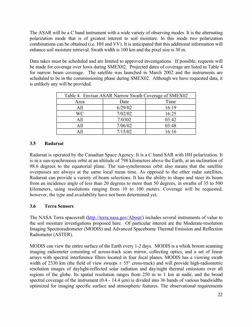
The ASAR will be a C band instrument with a wide variety of observing modes. It is the alternating polarization mode that is of greatest interest to soil moisture. In this mode two polarization combinations can be obtained (i.e. HH and VV). It is anticipated that this additional information will enhance soil moisture retrieval. Swath width is 100 km and the pixel size is 30 m. Data takes must be scheduled and are limited to approved investigations. If possible, requests will be made for coverage over Iowa during SMEX02. Projected dates of coverage are listed in Table 4 for narrow beam coverage. The satellite was launched in March 2002 and the instruments are scheduled to be in the commissioning phase during SMEX02. Although we have requested data, it is unlikely any will be provided.

Table 4. Envisat ASAR Narrow Swath Coverage of SMEX02 Area Date Time All 6/29/02 16:19 WC 7/02/02 16:25 All 7/0302 03:42 All 7/06/02 03:48 All 7/15/02 16:16

3.5 Radarsat Radarsat is operated by the Canadian Space Agency. It is a C band SAR with HH polarization. It is in a sun-synchronous orbit at an altitude of 798 kilometers above the Earth, at an inclination of 98.6 degrees to the equatorial plane. The sun-synchronous orbit also means that the satellite overpasses are always at the same local mean time. As opposed to the other radar satellites, Radarsat can provide a variety of beam selections. It has the ability to shape and steer its beam from an incidence angle of less than 20 degrees to more than 50 degrees, in swaths of 35 to 500 kilometers, using resolutions ranging from 10 to 100 meters. Coverage will be requested, however, the type and availability have not been determined yet. 3.6 Terra Sensors The NASA Terra spacecraft (http://terra.nasa.gov/About/) includes several instruments of value to the soil moisture investigations proposed here. Of particular interest are the Moderate-resolution Imaging Spectroradiometer (MODIS) and Advanced Spaceborne Thermal Emission and Reflection Radiometer (ASTER). MODIS can view the entire surface of the Earth every 1-2 days. MODIS is a whisk broom scanning imaging radiometer consisting of across-track scan mirror, collecting optics, and a set of linear arrays with spectral interference filters located in four focal planes. MODIS has a viewing swath width of 2330 km (the field of view sweeps ± 55° cross-track) and will provide high-radiometric resolution images of daylight-reflected solar radiation and day/night thermal emissions over all regions of the globe. Its spatial resolution ranges from 250 m to 1 km at nadir, and the broad spectral coverage of the instrument (0.4 - 14.4 µm) is divided into 36 bands of various bandwidths optimized for imaging specific surface and atmospheric features. The observational requirements

22

also lead to a need for very high radiometric sensitivity, precise spectral band and geometric registration, and high calibration accuracy and precision. Coverage time is about 16:15 UTC. Dates are summarized in Table 5. ASTER can obtain high-resolution (15 to 90 m) images of the Earth in the visible, near-infrared (VNIR), shortwave-infrared (SWIR), and thermal-infrared (TIR) regions of the spectrum. ASTER consists of three distinct telescope subsystems: VNIR, SWIR, and TIR. It is a high spatial, spectral, and radiometric resolution, 14-band imaging radiometer. Spectral separation is accomplished through discrete bandpass filters and dichroics. Each subsystem operates in a different spectral region and has its own telescope. Unlike the other instruments aboard Terra, ASTER does not collect data continuously; rather, it will collect an average of 8 minutes of data per orbit. ASTER data takes must be requested and potential coverage is limited by the satellite track and repeat.

Table 5. Terra MODIS Coverage for SMEX02 Date Track Frame Date Track Frame

June 21 20 31 July 7 20 31 June 23 18 31 July 9 18 31 June 28 21 31 July 14 21 31 June 30 19 31 July 16 19 31

3.7 Landsat Thematic Mapper The Landsat Thematic Mapper (TM) satellites collect data in the visible and infrared regions of the electromagnetic spectrum. Data are high resolution (30 m) and are very valuable in land cover and vegetation parameter mapping. Band 8 (panchromatic) for Landsat 7 has a 10 m resolution. Additional details on the Landsat program and data can be found at http://geo.arc.nasa.gov/sge/landsat/landsat.html. The Iowa site is located on both path 26 and 27 row 31. For path 27 the northern portion is not well covered, however, the Walnut Creek area is included. It may be necessary to acquire row 30 for complete coverage. At the present time coverage by both the Landsat 5 and 7 satellites results in frequent temporal coverage. Coverage dates are listed in Table 6 and shown in Figure 2.

Table 6. Landsat TM Coverage for SMEX02 Date Landsat No. Path Date Landsat No. Path

May 13 5 27 June 15 7 26 May 14 7 26 June 22 7 27 May 21 7 27 June 23 5 26 May 22 5 26 June 30 5 27 May 29 5 27 July 1 7 26 May 30 7 26 July 8 7 27 June 6 7 27 July 9 5 26 June 7 5 26 July 16 5 27 June 14 5 27 July 17 7 26

23

Figure 2. Map showing the SMEX02 region and Landsat TM frame coverage. Blue lines are Landsat scenes, gray area is the SMEX02 region and black lines are Ease Grids. The yellow box is 50 km by 50 km and is used to represent scale.

24

3.8 Advanced Very High Resolution Radiometer (AVHRR) This is a TIROS-N series satellite designed to operate in a near-polar, sun-synchronous orbit. During SMEX02 it is anticipated that 2 satellites may be providing AVHRR data Currently these NOAA 15 (morning coverage) and NOAA 16 (afternoon coverage). The AVHRR sensor collects data in the visible and infrared regions of the electromagnetic spectrum (see Table 7) and has a spatial resolution of approximately 1 km. Additional information on these data can be found at http://www.saa.noaa.gov/. Data can be acquired in three formats from the satellite. High Resolution Picture Transmission (HRPT) data are full resolution image data transmitted to a ground station as they are collected. The average instantaneous field-of-view of 1.4 milliradians yields a HRPT ground resolution of approximately 1.1 km at the satellite nadir from the nominal orbit altitude of 833 km (517 mi). Local Area Coverage (LAC) are full resolution data that are recorded on an onboard tape recorder for subsequent transmission during a station overpass. Resolution is the same as HRPT. Global Area Coverage (GAC) data are derived from a sample averaging of the full resolution AVHRR data. Four out of every five samples along the scan line are used to compute one average value and the data from only every third scan line are processed, which results in a 1.1 km by 4 km resolution

Table 7. AVHRR Bands Band No. Wavelengths

(micrometers) 1 0.58 - 0.68 2 0.725 - 1.10 3 3.55 - 3.93 4 10.3 - 11.3 5 11.5 - 12.5

3.9 Geostationary Operational Environmental Satellites (GOES) GOES satellites provide continuous monitoring in selected visible and infrared electromagnetric channels. Coverage of Iowa is currently provided by GOES-8. Of particular interest to this project is the imager. This is a multichannel instrument (see Table 8) that senses radiant energy and reflected solar energy from the Earth's surface and atmosphere. The resolution is 1 km for the visible and 4 km for the infrared channels. Additional information can be found at http://www.saa.noaa.gov/.

Table 8. GOES Imager Bands Band No. Wavelengths

(micrometers) 1 0.65 2 3.9 3 6.7 4 11 5 12

25

3.10 SeaWinds QuikSCAT SeaWinds is a radar scatterometer on QuikSCAT. It was launched in 1999 and was designed to measure near-surface wind speed over the Earth's oceans. A second instrument is scheduled to be launched on ADEOS-2 in November of 2002, and is expected to be operational by mid-2003. SeaWinds uses a rotating dish antenna with two spot beams that sweep in a circular pattern. The antenna spins at a rate of 18 rpm, scanning two pencil-beam footprint paths at incidence angles of 46o (H-pol) and 54o (V-pol). The antenna radiates microwave pulses at a frequency of 13.4 gigahertz across broad regions on Earth's surface with an 1800 km swath. QuikSCAT sampling at the latitude of Iowa is approximately two times daily; and ADEOS-2 is anticipated to have similar coverage. QuikSCAT is in a sun-synchronous, 803-kilometer, circular orbit with a local equator crossing time at the ascending node of 6:00 A.M. +/- 30 minutes. The SeaWinds antenna footprint is an ellipse approximately 25-km in azimuth by 37-km in the look (or range) direction. There is considerably overlap of these footprints, with approximately 8-20 of these ellipses with centers in a 25x25 km box on the surface. Signal processing provides commandable variable range resolution of approximately 2- to 10-km. The nominal resolution is approximately 6 km—an effective range gate of 0.5 msec. Additional information is available at http://podaac.jpl.nasa.gov/quikscat/qscat_doc.html. Gridded (0.2x0.2 degree) daily observations are available through BYU. Documentation is available at http://podaac.jpl.nasa.gov:2031/DATASET_DOCS/dLongSigBrw.html, and data orders can be placed through linked pages. Non-binned data are available, on tapes and through FTP, from the PO.DAAC (http://podaac.jpl.nasa.gov/quikscat/qscat_data.html).

26

4 AIRCRAFT REMOTE SENSING INSTRUMENTS Aircraft remote sensing will include visible, infrared, and microwave instruments. Visible and infrared measurements will be provided by the Utah State University aircraft over the watershed area. A total of four different aircraft microwave instruments may contribute to SMEX02. Two of these instruments are very important to the broad objectives of the experiment: PALS and PSR. The inclusion of the new two dimensional synthetic aperture radiometer is also a very high priority. Descriptions of these instruments are provided in the following sections. 4.1 Polarimetric Scanning Radiometer (PSR) The PSR is an airborne microwave imaging radiometer operated by the NOAA Environmental Technology Laboratory (Piepmeier and Gasiewski 2001) for the purpose of obtaining polarimetric microwave emission. It has been successfully used in several major experiments including SGP99 (Jackson et al. 2002). A typical PSR aircraft installation is comprised of four primary components: 1) scanhead, 2) positioner, 3) data acquisition system, and 4) software for instrument control and operation. The scanhead houses the PSR radiometers, antennas, video and IR sensors, A/D sampling system, and associated supporting electronics. The scanhead can be rotated in azimuth and elevation to any arbitrary angle. It can be programmed to scan in one of several modes, including conical, cross-track, along-track, and spotlight. The positioner supports the scanhead and provides mechanical actuation, including views of ambient and hot calibration targets. The PSR data acquisition system consists of a network of four computers that record several asynchronously-sampled data streams, including navigation data, aircraft attitude, scanhead position, radiometric voltage, and calibration target temperatures. These streams are available in-flight for quick-look processing. During SMEX02, the PSR/CX scanhead will be integrated onto the NASA WFF P-3B aircraft in the aft portion of the bomb bay. The PSR/CX scanhead is an upgraded version of the previously successful PSR/C scanhead used during SGP99 (Figure 3 and Table 9). The installation will utilize the NOAA P-3 bomb bay fairing, and will locate the PSR immediately aft of the NASA GSFC ESTAR L-band radiometer. The upload will commence at NASA WFF as soon as possible after the P3-B returns from the mission scheduled before SMEX02. The PSR/CX scanhead will have the polarimetric channels listed in Table 8 for SMEX02. The system will be operated in two imaging modes, both using conical scanning. Mapping characteristics are described in Table 10. Figure 4 shows the results of one day of mapping brightness temperature using the PSR in SGP99. At the end of a each set of flight lines a steep (~60 degree) port roll will be requested for the purpose of calibrating the PSR radiometers using cold sky looks. Additional details on the PSR not presented here can be found at http://www1.etl.noaa.gov/radiom/psr/.

27

Figure 3. PSR/C scanhead installed on the NASA P3-B aircraft during the SGP99 experiment.

Table 9. PSR/CX Channels for SMEX02 Frequency (GHz) Polarizations Beamwidth

5.82-6.15 V,h 10o 6.32-6.65 V,h 10o

6.75-7.10 * v,h,U,V 10o 7.15-7.50 V,h 10o

10.6-10.8 * v,h,U,V 7o 10.68-10.70 * V,h 7o

9.6-11.5 um IR V+h 7o * Indicates close to an AMSR-E channel.

28

Table 10. PSR Flightline and Mapping Specifications for SMEX02

Wide Area Imaging High-Resolution Imaging

Location Iowa Region Walnut Creek Watershed Site

Altitude (AGL) in m 7300 1800 Number of parallel flight lines 4 4 Flight line length (km) 150 50 Flight line spacing (km) 19 4.75 Scan period (seconds) 8 3 Incidence angle (deg) 55 55 3-dB footprint resolution 3.0 km at 6 GHz

2.0 km at 10 GHz 750 m at 6 GHz 500 m at 10 GHz

Sampling Oversampling above Nyquist

Nyquist

Figure 4. SGP99 PSR/C conically-scanned brightness temperature imagery 7.325 GHz channel, H-polarization, North looking.

29

4.2 Passive and Active L and S Band Microwave Instrument (PALS) In order to evaluate the potential of alternative approaches to soil moisture retrieval, a new L and S band integrated passive/active instrument has been developed (http://eis.jpl.nasa.gov/msh/mission+exp/pals.html) (Figure 5). PALS provides single beam observations at L and S bands, dual polarized, passive and active simultaneously (radar is polarimetric). The incidence angle is selectable between 30 and 50 degrees. Additional details are described in Table 11. This instrument offers many interesting opportunities for algorithm development and evaluation that have not been available; dual polarization, off nadir viewing typical of conical scanning systems, multifrequency, and both active and passive observations. From these observations we hope to obtain a better understanding of the frequency and polarization characteristics of land surfaces in the L to C-band range, leading to potential improvements in future spaceborne system designs and retrieval algorithms. Additional details on PALS can be found in Wilson et al. (2001). The PALS instrument was flown successfully in SGP99. Figure 6 shows a map product data set generated from the PALS data. PALS will be flown at low altitudes in SMEX02 over the Walnut Creek watershed flightlines.

Table 11. Description of the JPL PALS Instrument Parameter Radiometer Radar Frequencies 1.41 and 2.69 GHz 1.26 and 3.15 GHz Polarization V and H VV, VH, HH Sensitivity 0.2 K 0.2 dB Incidence angle 30 to 50 deg (preselected) 30 to 50 deg (preselected) Spatial resolution (@ 1000 m alt)

400 m 400 m

Figure 5. PALS antennas installed on the NCAR C-130 during SGP99. 30

TB LH Sigma0 LVV

July 09

July 11

July 12

July 13

July 14

210 220 230 240 250 260 270 280 290

Kelvin

Longitude

-98.30 -98.20 -98.10 -98.00

34.95

34.91

-98.30 -98.20 -98.10 -98.00

34.95

34.91

-98.30 -98.20 -98.10 -98.00

34.95

34.91

-98.30 -98.20 -98.10 -98.00

34.95

34.91

-98.30 -98.20 -98.10 -98.00

34.95

34.91

-98.30 -98.20 -98.10 -98.00

34.95

34.91

-98.30 -98.20 -98.10 -98.00

34.95

34.91

-98.30 -98.20 -98.10 -98.00

34.95

34.91

-98.30 -98.20 -98.10 -98.00

34.95

34.91

-98.30 -98.20 -98.10 -98.00

34.95

34.91

Latit

ude

dB-23 -21 -19 -17 -15 -13

Figure 6. PALS brightness temperature and radar backscatter image products from SGP99. 4.3 Electronically Scanned Thinned Aperture Radiometer (ESTAR) ESTAR is a synthetic aperture, passive microwave radiometer operating at a center frequency of 1.413 GHz and a bandwidth of 20 MHz. As installed in the SMEX02 mission it is horizontally polarized. Aperture synthesis is an interferometric technique in which the product (complex correlation) of the output voltage from pairs of antennas is measured at many different baselines. Each baseline produces a sample point in the Fourier transform of the scene, and a map of the scene is obtained after all measurements have been made by inverting the transform. ESTAR is a hybrid real and synthetic aperture radiometer that uses real antennas (stick antennas) to obtain resolution along-track and aperture synthesis (between pairs of sticks) to obtain resolution across-track (Le Vine et al., 1994). This hybrid configuration could be implemented on a spaceborne platform. The effective swath created in the ESTAR image reconstruction (essentially an inverse Fourier transformation) is about 45o wide at the half power points. The field of view is restricted to 45o to avoid distortion of the beam but could be extended to wider angles if necessary. The image reconstruction algorithm in effect scans this beam across the field of view in 2o steps. The beam width of each step varies depending on look angle from 8 to 10o, therefore, the individual original data are not independent, since each data point overlaps its neighbors. Contiguous beam positions can be achieved by averaging the response of several of these data points. This results in approximately nine independent beam positions. For this experiment the swath will be restricted to approximately 35o. Another approach to using the data, especially in a mapping mode, is to interpret each of the original nonindependent observations as a sample point and then use a grid overlay to average the data. The final product of the ESTAR is a time referenced series of data consisting of the set of beam position brightness temperatures at 0.25 second intervals.

31

Calibration of the ESTAR is achieved by viewing two scenes of known brightness temperature. By plotting the measured response against the theoretical response, a linear regression is developed that corrects for gain and bias. Scenes used for calibration include black body, sky, and water. During aircraft missions, a black body is measured before and after the flight and a water target during the flight. Water temperature is determined using a thermal infrared sensor. The match in level and pattern is quite good and in general the ESTAR calibration should be considered accurate and reliable. For interpretation purposes it should be noted that the sensitivity of soil moisture to brightness temperature is 1% for 3oK. ESTAR has demonstrated the potential of L band radiometry and STAR technology (Levine et al. 1994 and 2001, Jackson et al., 1995 and 1999). Figure 7 is an example of the type of product produced after processing the ESTAR data. Details on ESTAR and soil moisture products can be found at the following web site http://daac.gsfc.nasa.gov/CAMPAIGN_DOCS/SGP97/estar.html. Including ESTAR in SMEX02 is important because it will extend the range of vegetation types that the instrument has been applied to and it will complement the AIRSAR for data fusion and integrated algorithm studies.

32

Figure 7. ESTAR brightness temperature image from the SGP97 experiment (Jackson et al. 1999).

4.4 Airborne Synthetic Aperture Radar (AIRSAR) AIRSAR is a side-looking radar instrument developed by the Jet Propulsion Lab http://airsar.jpl.nasa.gov/. It has several operating modes. In SMEX02 the polarimetric (POLSAR) will be used. In POLSAR mode, fully polarimetric data are acquired at all three frequencies C-, L-, and P-band. Fully polarimetric means that radar waves are alternatively transmitted in horizontal (H) and vertical (V) polarization, while every pulse is received in both H and V polarizations. Therefore, there are four combinations; HH, VV, HV and VH. Basic parameters of the AIRSAR are listed in Table 12. It is anticipated that the 20 MHz bandwidth data will be requested.

Table 12. AIRSAR Parameters Channel C L P Frequency GHz 5.29875 1.2375 0.4275Pixel Spacing 20 MHz Bandwidth (m) 10 x 10 Swath Width 20 MHz Bandwidth m 15 Pixel Spacing 40 MHz Bandwidth (m) 5 x 5 Swath Width 40 MHz Bandwidth (m) 10

4.5 Global Positioning System (GPS) Reflectivity Technique The GPS satellite constellation currently broadcasts a civilian-use carrier signal at 1575.42 MHz, which is bi-phase modulated by satellite-specific pseudorandom noise codes. The signals are encoded with timing and navigation information so that the receiver can calculate the positions of the transmitting satellites and solve for its own position and time by measurement of pseudoranges from at least four satellites. These direct signals (Figure 8) are normally received by a low-gain, hemispherical, zenith antenna. These same GPS signal transmissions also reflect off of the Earth's surface and can be measured with a nadir-viewing antenna at longer delays than the direct signal. The reflected signal is modified by the roughness and dielectric properties of the scattering surface. If the roughness is known a priori or is assumed constant over some time, the ratio of reflected signal power to the direct signal power is an indicator of the dielectric constant of the surface. Therefore, this ratio can be used to temporally sense changes in soil moisture in the top 5 cm of the surface. Additionally, the polarization of the RHCP direct signal is predominantly LHCP upon surface reflection for most incidence angles. Because the geometry is variable depending upon the slowly changing transmitter and receiver positions, a hemispherical nadir antenna has been used in past ocean reflection research. In SMEX02, a higher gain nadir antenna is anticipated to achieve a better SNR at the expense of tracking multiple satellites. The received signals are cross-correlated with a replica signal (1 ms code length) to produce a narrower, approximate 1 µs correlation pulse. This procedure is similar in design to pulse compression radar receivers. Our previous efforts have been focused on the distribution or spreading of the reflected signal power over time delay, which is an indicator of the roughness of the reflecting surface. For soil moisture sensing, the observable is the ratio of the magnitudes of the reflected and direct signal powers.

33

Rough surface glistening zone

Range cells

GPS Transmitters24 sats

L1: 1.5, L2: 1.2 GHzPRN coding

Direct SignalRCP

Reflec

ted S

ignal

LCP

GPS ReceiverZenith & nadir antennas

)sin(2 θδ

≈h

θRough surface glistening zone

Range cells

GPS Transmitters24 sats

L1: 1.5, L2: 1.2 GHzPRN coding

Direct SignalRCP

Reflec

ted S

ignal

LCP

GPS ReceiverZenith & nadir antennas

GPS ReceiverZenith & nadir antennas

)sin(2 θδ

≈h

θ

Figure 8. Bistatic radar configuration of reflected GPS signals.

In bistatic radar systems, scattering is mainly forward, and the radar cross section is expressed as a normalized bistatic cross section. For the specific case of an aircraft receiving direct and land-reflected GPS signals, we use an analytical scattering model developed by Zavorotny and Voronovich (Z-V model) (2000). The model is based upon physical optics and will employ a rough surface estimated from the SMEX02 terrain. The current GPS bistatic radar receiver is based upon a modified Plessey 12-channel C/A code receiver built by NASA Langley Research Center. New receivers are currently being developed for GPS bistatic radar applications, and their use in SMEX02 is possible. The Plessey receiver is comprised of a single board containing two RF front-ends and a correlator, which is connected to a PC-104 computer in a small, lightweight chassis (20x15x15 cm). The RF front-ends perform automatic gain control, down conversion, and IF sampling. The PC-104 computer serves as the controller and data logger for both GPS navigation functions and recording the signal power. The GPSBuilder-2 software allows access to the correlator power measurements. In the Delay Mapping Receiver (DMR) mode of operation, five channels track direct signals in a conventional, closed-loop fashion. The pseudorange and Doppler measurements made by these channels are used to form navigation solutions. The other 14 correlators (two for each of seven channels) are controlled in an open-loop mode to measure reflected signal power at specific delays relative to one or more of the direct signal channels. For each of the slaved reflection correlators, one hundred 1 ms correlator samples are averaged to produce an estimate of reflected signal power at a rate of 10 Hz. The reflected signal power is sampled in discrete bins around

34

the time delay corresponding to the arrival of the signal from the specular reflection point. The direct and reflected signal power measurements are stored on internal disk for later analysis. In the DMR mode of operation, the bistatic radar receiver can operate for long periods without user intervention. In SMEX02, the GPS bistatic radar receiver will operate as a proof-of-concept technology onboard the NCAR C-130 aircraft. The GPS-based measurements will be evaluated in conjunction with the observations made by the JPL PALS instrument and the ground sampling of soil moisture. The GPS bistatic radar measurement parameters are presented in Table 13. These tests will guide future development of optimized receivers and processing algorithms to retrieve soil moisture and surface roughness information from GPS bistatic radar measurements.

Table 13. GPS Bistatic Radar Parameters Parameter GPS Bistatic Radar Frequency 1.56 GHz

Polarization LHCP Incidence Angle 0-60 deg (predicted by satellite geometry)

Spatial Resolution Variable w/ height & angle (first Fresnel zone) The GPS instrument research will be conducted by the Colorado Center for Astrodynamics Research at the University of Colorado at Boulder. For more information on GPS remote sensing using land and ocean reflections, visit http://ccar.colorado.edu/~dmr.

4.6 Utah State University Visible and Infrared Airborne System The Remote Sensing Services Laboratory at Utah State University (USU) will support the experiment with a series of over flights using its airborne system of short wave and long wave imagers mounted in a light twin-engine Piper Seneca II. The system consists of three Kodak Megaplus 4.2i digital cameras, with interference filters forming narrow spectral bands centered in the green (0.55 µm), red (0.67 µm) and near-infrared (0.80 µm) portions of the electromagnetic spectrum. These filters are interchangeable so different bandwidths could be used for this experiment if desired by the research community involved. An onboard GPS system is used to navigate along pre-planned flight lines over the site, as well as to geo-reference the approximate center of each set of digital images. The cameras are mounted inside a specially designed graphite composite cylinder with adjustable aluminum mounts that are installed through a hole in the belly of a Piper Seneca II twin-engine aircraft. The adjustable mounts allow for the alignment of the cameras, which are usually set to view a very distant target. The system also supports an Inframetrics 760 thermal infrared scanner that is mounted through a separate porthole for the acquisition of thermal infrared imagery in the 8 - 12 µm range. This imagery is stored on S-VHS videotape and later frame-grabbed in the laboratory. A color video camera is used to acquire color imagery of the flight. GPS position information is encoded on the bottom of this imagery, which are also stored on videotape.

35

5 REMOTE SENSING AIRCRAFT MISSION DESIGN The PSR and ESTAR instruments will be installed on the NASA WFC P3-B aircraft. PALS will be installed on a C-130 aircraft operated by NCAR (http://raf.atd.ucar.edu/). A GPS instrument will be part of the C-130 instrumentation and there may also be one on the P3-B. AIRSAR operates from the DC-8. An aircraft briefing will be conducted each night at the hotel selected in Des Moines (Embassy Suites). Arrangements will be made for a phone link to a single location in Ames to allow communication with any aircraft operations based there. As in previous missions, the goals of the experiment design are to collect data for both algorithm development/verification and soil moisture mapping. The extent and scale of the mapping must satisfy the range of objectives of the land-atmosphere and AMSR components of SMEX02. Unlike recent experiments, low altitude flightlines will be emphasized. The following sections describe the flight missions of the five aircraft that will take part in SMEX02. 5.1 NCAR C-130 This aircraft is operated by the National Center for Atmospheric Research (NCAR). Details on the aircraft can be found at http://raf.atd.ucar.edu/. It will have the PALS and GPS sensor systems on board. In addition, there is meteorological instrumentation available on the aircraft that may be of value. The primary mission of the C-130 is to fly low altitude flightlines over the Walnut Creek Watershed area with the PALS instrument. The mission design is similar to SGP99. It will utilize a series of basically East-West lines. These are 800 m apart and offset from the road network by 400 m. Roads are approximately on a square 1600 m grid. With a nominal field size of 800 m and sensor footprint size of 400 m, this procedure provides a reliable sample for the study sites and allows interpolation for mapping. The flightlines are listed in Table 14 and shown in Figure 9. In past experiments, these types of lines have been flown sequentially in alternating East-West directions. However, the investigators may encounter local RFI and may need to alter the sequencing or design. In SGP99, the RFI was directional and all lines had to be flown in a single direction. The major impact of this type of change is on flight hours. If longer individual flights are required it may be necessary to reduce the number of flights. Flights will be conducted in the morning. Each flight will be approximately 2.5 hours in duration. It is anticipated that nine flights will be conducted. The aircraft is expected to arrive in Des Moines on Thurs. June 20 and be based out of DMS airport. It is scheduled to depart on July 8.

36

Figure 9. SMEX02 Walnut Creek watershed area and microwave aircraft flightlines. Blue lines are the low altitude microwave flightlines; yellow squares indicate intensive soil moisture sampling sites (those with red text are also flux tower sites). The large yellow square is 2 km by 2 km and is used to illustrate scale.

Table 14. SMEX02 C-130 Flightlines Line No.

Altitude (km)

Length (km)

Description Start Lat. Start Lon. Stop Lat. Stop Lon.

1 1 33 C-130 41.925 -93.4 41.925 -93.8 2 1 33 C-130 41.932 -93.8 41.932 -93.4 3 1 33 C-130 41.940 -93.4 41.940 -93.8 4 1 33 C-130 41.947 -93.8 41.947 -93.4 5 1 33 C-130 41.954 -93.4 41.954 -93.8 6 1 33 C-130 41.962 -93.8 41.962 -93.4 7 1 33 C-130 41.969 -93.4 41.969 -93.8 8 1 33 C-130 41.976 -93.8 41.976 -93.4 9 1 33 C-130 41.983 -93.4 41.983 -93.8 10 1 33 C-130 41.991 -93.8 41.991 -93.4

5.2 NASA P-3B The P-3B operates from the NASA Wallops Flight Facility in Wallops Island, VA. Details on the aircraft can be found at http://www.wff.nasa.gov/. It will have the PSR and ESTAR sensor systems on board. There may also be a GPS sensor system installed during SMEX02. The primary mission of the P3-B is to collect both low and high altitude data over the Iowa study region with the PSR instrument. High altitude lines are more important than the low altitude lines.

37

Another very important objective is to collect data with the ESTAR over the region. Mission design and operations are dependent on the PSR and not the ESTAR. Flightlines are listed in Table 15 and plotted in Figure 10. The low altitude and water calibration lines correspond to those listed for the C-130. High altitude lines will provide coverage of an area that is approximately 40 km wide (East-West) and 95 km long (North-South).

Table 15. SMEX02 P-3B Flightlines Line No.

Altitude (km)

Length (km)

Description Start Lat. Start Lon. Stop Lat. Stop Lon.

3 1.5 33 P3-B 41.940 -93.4 41.940 -93.8 7 1.5 33 P3-B 41.969 -93.4 41.969 -93.8

11 8.5 95 P3-B 41.75 -93.7 42.7 -93.7 12 8.5 95 P3-B 42.7 -93.567 41.75 -93.567 13 8.5 95 P3-B 41.75 -93.433 42.7 -93.433 14 8.5 95 P3-B 42.7 -93.3 41.75 -93.30

15 0.5 12 Water Calibration 41.6756 -93.6648 41.7813 -93.7279 Flights will be conducted during the mid day in order to match the nominal Aqua overpass time of 1330. Each flight will be approximately 2.5 hours in duration. It is anticipated that eleven high altitude flights will be conducted. The aircraft is expected to arrive in Des Moines on Mon. June 24 and be based out of DMS airport. It is scheduled to depart on July 12. 5.3 NASA DC-8 The AIRSAR instrument will be flown on NASA's Douglas DC-8. This is a four jet engine aircraft operated out of the Dryden Flight Center in California http://www.dfrc.nasa.gov/airsci/dc-8/dc8page.html. AIRSAR flights for SMEX02 will be flown at an altitude of 8 km. The primary mission of the DC-8 is to collect AIRSAR data close in time with passive microwave measurements made by instruments on the C-130 and P-3B aircraft. The objectives of including AIRSAR in SMEX02 are:

• Collect AIRSAR and passive microwave observations (PALS, ESTAR, and PSR) at

different spatial resolutions that will allow the validation of passive and active data fusion concepts.

• Collect AIRSAR observations concurrent with high quality ground observations over a range of soil moisture and vegetation conditions that will allow the extension and validation of the current radar soil moisture algorithms to vegetated surfaces with higher biomass levels.

• Obtain AIRSAR observations concurrent with Envisat ASAR, ERS-2 and Radarsat measurements to evaluate the quality and value of these sensors in soil moisture applications

38

39

Figure 10. SMEX02 regional flightlines and mapping area. Regional mapping flightlines are indicated in black, regional soil moisture sites are shown as a red X. The yellow box is 10 km by 10 km and is used to illustrate scale.

In order to accomplish these objectives, we have prepared a flight with the following key features: • Flights between July 1 and July 8, 2002 in order to maximize overlap with PALS on the

C-130. It is also anticipated that we will be able to obtain data to capture several wet and dry conditions for corn and soybeans at different stages of growth. It is anticipated that there will be four flight dates. The arrival and departure dates can also be science data collection dates.

• Flights will be concentrated over the Walnut Creek Watershed, an area 10 km North-South and 40 km East-West where PALS and intensive ground sampling will be conducted. Swath coverage areas are summarized in Table 16 and illustrated in Figure 11. Multiple flightlines are desired in order to produce a composite image of the watershed with a nominal incidence angle range close to 40 degrees (the PALS and proposed HYDROS incidence angle). This will facilitate the disaggregation studies and use with PALS. In addition, this design will result in multiple incidence angle observations over the test sites, which will allow the exploration of new algorithm concepts. Note that the flightlines are defined by swath corners.

• Regional coverage data sets will be collected for extrapolation of the watershed results to larger scales typical of satellite radiometer footprints. Swath coverage areas are summarized in Table 16 and illustrated in Figure 11.

• If Envisat data can be scheduled, concurrent flights will be made to acquire Envisat ASAR data during SMEX02.

• Flights will be conducted between 1100 and 0100 local time. It is possible that the radar could contaminate the passive measurements being made on the C-130 and the P-3. Therefore, the aircraft will be scheduled to reduce this possibility.

Table 16. NASA DC-8 AIRSAR Flightline Parameters

Swath Corners (Degrees) Flight line

Altitude (km)

Flight Heading (Deg.)

Length (km)

Latitude Longitude

Latitude Longitude

Latitude Longitude

Latitude Longitude

1 8 180 110 41.74823 41.74823 42.7026 42.7026 -93.5634 -93.3082 -93.5653 -93.3063

2 8 360 110 41.74823 41.74823 42.7026 42.7026 -93.7962 -93.5411 -93.7981 -93.5391

3 8 90 60 41.89276 42.08381 41.89276 42.08381 -93.2379 -93.2379 -93.962 -93.962

4 8 90 60 41.91476 42.1058 41.91476 42.1058 -93.2365 -93.2365 -93.9634 -93.9634

5 8 270 60 42.00123 41.81018 42.00123 41.81018 -93.9647 -93.9647 -93.2354 -93.2354

6 8 270 60 42.02324 41.83219 42.02324 41.83219 -93.966 -93.966 -93.2341 -93.2341

40

41

Figure 11. SMEX02 AIRSAR coverage areas. Regional study area is outlined as red/black. The watershed area will be covered by four swaths. A larger region will also be mapped by two North-South swaths.

5.4 Canadian Twin Otter The Twin-Otter aircraft (Figure 12) operated by personnel from the National Research Council of Canada (MacPherson et al., 2001) will be available for making aircraft-based flux observations over several transects surrounding the watershed. Surface layer flux measurements (~30 m agl) will be conducted using an east-west transect starting west of the watershed and ending west of the interstate (Figure 13 and Table 17). The frequency and timing of the flux-aircraft observations will be subject to the flying schedule for the microwave observations. Ideally, flights in the mid-morning (~1030 local time), around the time of EOS Terra and Landsat 7 overpasses, would be the most useful. Mid-morning is also the typical time for the ALEXI output and when the frequency of clouds via boundary layer convective activity is minor. With length of the flight transects ~ 20 km and flying at ~30 m agl, transect-average fluxes represent aggregated values of length scales ~ 10 km. However, sub-sampling the transects for comparisons with tower-based observations has also been successful.

Figure 12. Twin Otter atmospheric research aircraft configured for flux studies.

42

Figure 13. Twin Otter flightlines for SMEX02. Aircraft flux lines are in blue with letter codes. The yellow squares indicate sites with flux towers. The large yellow square is 2 km by 2 km and is used to illustrate scale.

Table 17. SMEX02 Twin Otter Flightlines

Line No.

Altitude (km)

Length (km)

Description Start Lat. Start Lon. Stop Lat. Stop Lon.

A .03 6.4 Aircraft Flux 41.94333 -93.66600 41.88600 -93.66600B .03 11.9 Aircraft Flux 41.92983 -93.78883 41.93300 -93.64466C .03 10.0 Aircraft Flux 41.95466 -93.75000 41.95833 -93.62900D .03 8.5 Aircraft Flux 41.97300 -93.65433 41.89683 -93.65433E .03 9.0 Aircraft Flux 41.97933 -93.74216 41.89833 -93.73950F .03 6.2 Aircraft Flux 41.99316 -93.70033 41.93850 -93.71516G .03 9.5 Aircraft Flux 42.00000 -93.76850 41.95733 -93.68083H .03 7.5 Aircraft Flux 41.97200 -93.73666 41.97200 -93.64616J .03 6.3 Aircraft Flux 41.93733 -93.53650 41.99333 -93.52600

5.5 Utah State University Piper Seneca High-resolution airborne multispectral imagery will be acquired with the USU airborne digital system (Neale and Crowther, 1994). Christopher Neale will coordinate missions with NCAR C-130, NASA WFC P3-B, NASA DC-8 and Twin Otter teams. Short-wave imagery will be acquired over the study area from 3200 meters above ground level, using Nikon 20 mm lenses, resulting in a pixel size of approximately 1.5 meters. Each image consists of approximately 2000 x 2000 pixels, so the resulting swath will be 3.0 km. The flightlines, see Table 18, were planned to cover the entire study area, with a side overlap of 30% between imagery. Along each flight line, the images will be acquired with a 60% overlap to facilitate the mosaicking of the 43

imagery during post-processing. This flight line plan will result in approximately 128 images to be processed for each mission. The pixel resolution of the optical data will be ~ 1.5 m pixel size.

Table 18. Systematic Coverage of Walnut Creek Watershed Area Flightline Latitude Long. Start Latitude Long. End

U1 41.93111 93.8 41.93111 93.4 U2 41.95003 93.4 41.95003 93.8 U3 41.96894 93.8 41.96894 93.4 U4 41.98786 93.4 41.98786 93.8

The flight plan may vary for the different sensors, due to differences in the footprint of the short-wave band digital cameras and the thermal infrared Inframetrics scanner. It is expected during this period of rapid vegetation growth that there will be a need for a set of high-resolution short-wave imagery covering the study area at the beginning, middle and end of the experimental period to capture the changes in biomass and albedo throughout the period. USU will try and acquire imagery to coincide with the LANDSAT overpasses depending on the weather conditions. However, the thermal infrared image acquisition will be closely tied to the PALS and Twin Otter flights and will also include post-dawn flights with subsequent flights throughout the day to capture the thermal inertia of the system and for testing the time-rate-of-change algorithms at high pixel resolutions. Some transects at even higher pixel resolutions (~ 0.5 m) will be obtained (using lower flight lines) to capture the effects of incomplete covered vegetation systems and to aid in the calibration of the imagery. The optical images provide distributed surface cover characterizations that are necessary for calculation of water and energy exchange rates. Due to the high spatial resolution of the imagery, the system lends itself well to monitor sparse or incomplete cover crops, as it can resolve the soil background and vegetation canopy. The highest resolution imagery will support the ground measurements of LAI and fractional vegetation cover in certain cropped fields. These data add significant value to the planned soil moisture observations. The over flights are presently budgeted to cover approximately 17 hours of flight time over the site. The flights will be planned, usually for the morning hours to avoid excessive cloud cover, and to support different project activities that will include: • Systematic coverage of the larger research area with a combination of short wave (1.5

meter resolution) and long wave (5 meter resolution) measurements to coincide with airborne microwave flights (see Table 18, Figure 14). Flight altitude ~ 3200 m.

• Higher resolution (0.5 meter short wave, 1 meter long wave) imagery over the fields containing the flux stations and lidar equipment (see Table 19, Figure 14). Flight altitude ~ 1000 m.

• Higher resolution flight lines over sites where biophysical canopy properties will be measured and intensive soil moisture measurements will be conducted.

44

On the day of each flight, a calibrated barium sulfate reflectance panel with known bi-directional reflectance properties will be set up leveled at a central location within the study area. The incoming irradiance reflected by the panel will be continuously monitored using an Exotech 4-

Figure 14. Utah State University (USU) flightlines. Dashed lines are designed for mapping the watershed area and solid lines are for low altitudes flights over flux tower sites.

Table 19. USU Low Altitude Flightlines

Flightline Latitude

Start (Deg.)

Longitude Start

(Deg.)

Latitude Stop

(Deg.)

Longitude Stop

(Deg.) U5 41.9331 93.7667 41.9331 93.64 U6 41.9356 93.7667 41.9356 93.64 U7 41.9393 93.7667 41.9393 93.64 U8 41.9456 93.697 41.9456 93.634 U9 41.9493 93.697 41.9493 93.634 U10 41.9529 93.697 41.9529 93.634 U11 41.9586 93.69 41.9586 93.634 U12 41.9623 93.69 41.9623 93.634 U13 41.9722 93.75 41.9722 93.640 U14 41.9762 93.75 41.9762 93.640 U15 41.9798 93.65 41.9798 93.640 U16 41.9918 93.55 41.9918 93.515 U17 41.9881 93.55 41.9881 93.515 U18 41.9437 93.5481 41.9437 93.5222 U19 41.94 93.5481 41.94 93.5222

45

band radiometer with Thematic Mapper bands TM1-4 and a 21X data logger. The radiometer used will be the same instrument used to obtain the absolute calibration of the digital cameras in a separate lab experiment. The reflectance of some large uniform representative surfaces within the study area will also be measured to check the image calibration, using a second Exotech radiometer and Polycorder data logger. At the beginning or at the end of each flight mission, the aircraft will acquire thermal infrared imagery over a nearby reservoir, where water temperatures are routinely measured. These data will be used to check the accuracy of the surface temperature estimates and atmospheric corrections using MODTRAN. Three sets of flightlines will be utilized. Table 18 shows the systematic coverage of the watershed area, where the images will be acquired from 3200 meters above ground level (10500 feet). Considering the average ground elevation of the study area, the aircraft will be positioned at 11500 feet while acquiring images for these flight lines. The swath width of the short-wave imagery will be approximately 3000 meters. These image acquisition campaigns will coincide with the Landsat satellite overpasses whenever weather permits. We estimate a minimum of three and a maximum of six systematic coverage flights of the entire watershed study area. The lower elevation flightlines (Table 19) have been planned to cover the all the flux stations located within the experimental area. These are parallel east-west flight lines, spaced approximately 410 meters apart, covering the flux stations and the area to the south-southwest of each station, which is the prevailing upwind direction. Additional flight lines could be added to include important vegetation sampling and soil moisture monitoring sites. The flight elevation will be 1067 meters (3500 feet) above ground level, or 4500 feet. This will result in a short-wave image swath width of 1000 meters and a thermal swath width of 587 meters. These flight lines will be flown whenever the weather permits, at different times of the day. At least one pre-dawn campaign of these flight lines will be conducted for thermal inertia estimates. The third set of flightlines will be used to match several of the Twin Otter flightlines for matching fluxes at this scale. The lines selected are A, D, E, F, and J described in Table 17. These will be flown at an altitude of 2100 m. The swath width of the thermal imagery will be approximately 1200 m and the pixel size will be 2 m. The shortwave imagery will have a pixel size of 1 m. The USU team will arrive on June 12th to initiate the image acquisition. The campaign will be divided into two periods: (1) from June 12th to June 23rd and (2) from July 1st to July 9th. During the period from June 23rd to July 1st, the aircraft will return to Utah to obtain data for other committed projects as well as to have the annual inspection of the aircraft. The USU aircraft maintenance personnel will be pre-planning the purchase of items necessary for the annual inspection in order to expedite this procedure within three days.

46

6 IOWA STUDY REGION In order to satisfy the requirements of the diverse research projects making up SMEX02 it was necessary to include a test site that would provide a data set for the development and verification of alternative soil moisture retrieval algorithms under significant biomass levels associated with agricultural crops and satisfy the land atmosphere investigations described in other sections. It is essential that multi-parameter microwave observations be obtained over a range of soil moisture conditions with moderate to high vegetation biomass conditions. A study site in Iowa was selected. Within this region, is a small watershed, Walnut Creek just south of Ames, IA This watershed has been the focus of research by the USDA ARS National Soil Tilth Lab (NSTL) http://www.nstl.gov/. Nearly 95% of the region and watershed is used for row crop agriculture. Corn and soybean are grown on approximately 80% of the row crop acreage, with greater than 50% in corn, 40-45% in soybean and the remaining 5-10% in forage and grains. The watershed is representative of the Des Moines Lobe, which covers approximately 1/4 of the state of Iowa. The climate is humid; with an average annual rainfall of 835 mm. SMEX02 is tentatively planned from mid June through mid-July. At the outset corn will be in early stages of growth and most soybean fields will be essentially bare soil. By the end of June in a typical growing season, corn biomass is expected to range between 3 and 4 kg m-2, while soybean will have a biomass of less than 1 kg m-2. This translates to leaf-area index (LAI) values on the order of 2 and 0.5 and fractional canopy cover about 0.75 and 0.5 respectively, for corn and soybean. The area around central Iowa is considered the pothole region of Iowa because of the undulating terrain. This area on the Des Moines lobe represents the youngest of soils in the United States. Two features standout in this terrain. First, the lack of a surface stream channel except for the areas near streams and rivers. Second, the large variation of soil types within a field. Surface organic matter contents often range from 1-2 % to over 8% in a transect from the pothole areas to the eroded knolls within the same field. This is also coupled with a variation in rooting depth. These features create a potential condition in the spring and extremely wet summers of a soil surface covered with random water-filled potholes. Typically, however, these potholes are dry by early spring due to subsurface drainage and farmers are able to plant without any problems. This variation, however, presents a challenge when field sampling to ensure that the surface conditions within the field are adequately sampled. The NSTL has been developing a library of soils maps for a number of fields along with a differential GPS to measure topography at the 10-15 cm contour interval. Additional regional information can be found at the following sites http://mcc.sws.uiuc.edu/Introduction/micis.html and http://www.exnet.iastate.edu/Information/weather.html

47

The heaviest precipitation months are May and June (about 1/3 of the annual total) Rainfall events in the spring and summer are often thunderstorms, providing brief and intense showers. The topography is characterized by low relief and poor surface drainage. “Prairie potholes” are a common feature of the region. Figure 15 is one orthophoto image collected under bare soil

conditions that clearly illustrates this phenomena. The soils are loams and silty clay loams, with generally low permeability. Figure 16 shows the general soil texture distribution in the region. Anthropogenic forces have significantly modified the hydrologic character of the basin. Over the past 100 years most of the “prairie potholes” have been drained, much of the land cultivated and many of the agricultural fields have been tile drained to assist in subsurface drainage (tile flow). Conventional tillage is most widely used, however no tillage and ridge tillage have been recently introduced.

Figure 15. USGS orthophoto image from the Walnut Creek watershed area.

Figure 16. SMEX02 regional soil textures (green=loam and brown=silty clay loam). Within the Walnut Creek watershed area there are 20 recording rain gauges separated by 1-mile intervals or sections and air temperature is also recorded at these sites. There are two 48

meteorological stations located in the watershed measuring air temperature, relative humidity, wind speed and direction, soil temperature and solar radiation. There are five stream gauging locations in the watershed designed to isolate water flow and water quality for three sub-watersheds and the entire basin. Figures 2 and 10 show the regional study area. Figure 17 is a false color Landsat TM image obtained on July 27, 2000. Nearly all fields rotate between corn and soybeans each year; therefore, we expect to see a similar spatial pattern in 2002 (Bright red=soybeans and dark red=corn). Both row and drilled soybeans planting practices are in use. Figure 18 shows row soybean and corn conditions on June 27th 2000. Figure 19 is a higher resolution Landsat TM image of the watershed area. 6.1 Watershed Sites Sites were identified within the Walnut Creek watershed (code=WC) to satisfy the data requirement of the PALS and surface/aircraft flux components of the experiment. To the extent possible the sites selected had the following characteristics: • At least 800 m in the NS direction • At least 800 m in the EW direction • Centered on one of the low altitude C-130 flight lines • Single cover condition • Single management unit • Balance of corn and soybeans • Dominant soil types • Wind direction • Flux aircraft constraints • Geographic domain • Permission to use Figure 9 shows the locations plotted on a road map. Table 20 summarizes these sites and describes the expected crop type and row direction.

49

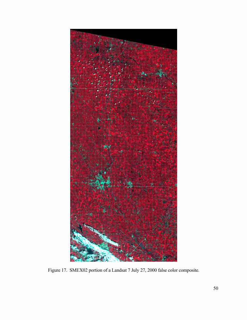
Figure 17. SMEX02 portion of a Landsat 7 July 27, 2000 false color composite.

50

a) b)

Figure 18. Walnut Creek, Iowa a) typical corn canopy and b) typical row soybeans on June 28, 2000.

51

Figure 19. SMEX02 Walnut Creek watershed portion of a Landsat 7 July 27, 2000 false color composite.

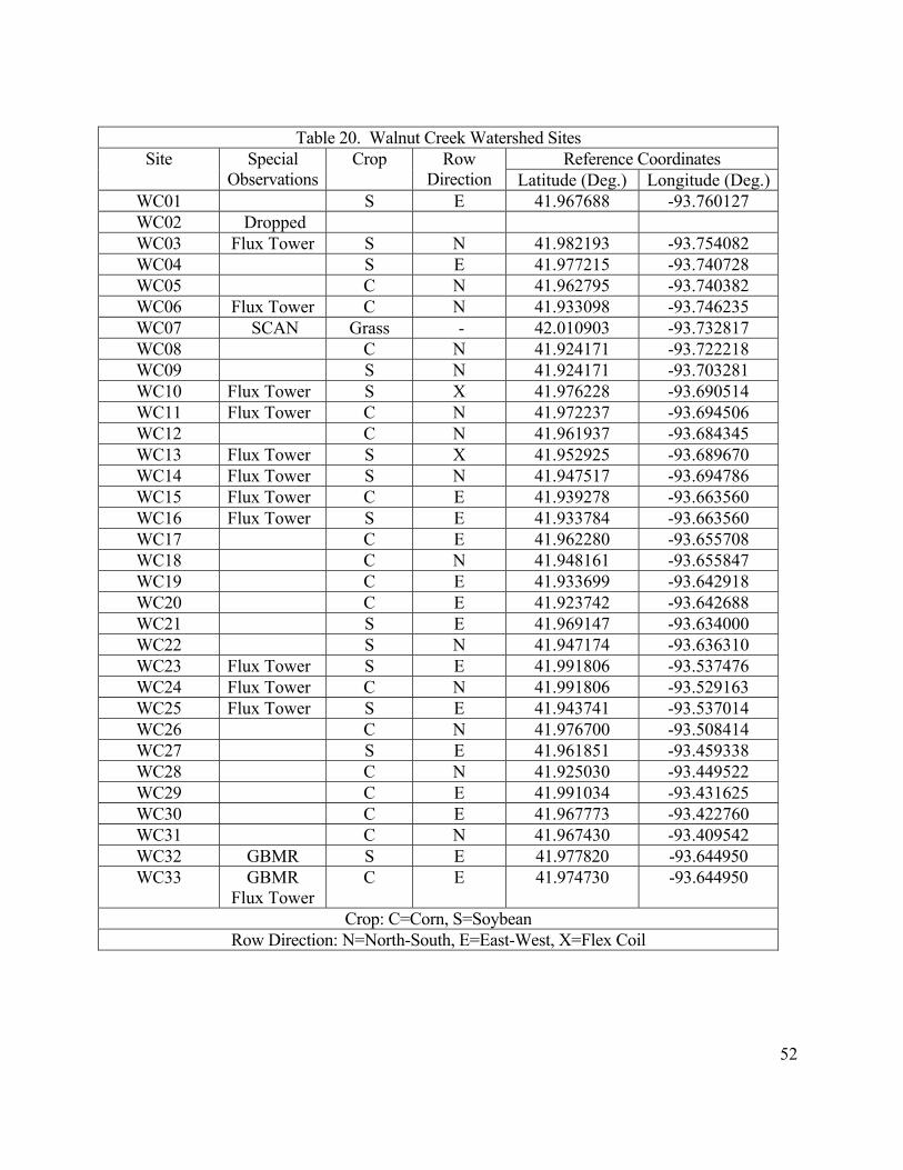
Table 20. Walnut Creek Watershed Sites

Reference Coordinates Site Special Observations

Crop Row Direction Latitude (Deg.) Longitude (Deg.)

WC01 S E 41.967688 -93.760127 WC02 Dropped WC03 Flux Tower S N 41.982193 -93.754082 WC04 S E 41.977215 -93.740728 WC05 C N 41.962795 -93.740382 WC06 Flux Tower C N 41.933098 -93.746235 WC07 SCAN Grass - 42.010903 -93.732817 WC08 C N 41.924171 -93.722218 WC09 S N 41.924171 -93.703281 WC10 Flux Tower S X 41.976228 -93.690514 WC11 Flux Tower C N 41.972237 -93.694506 WC12 C N 41.961937 -93.684345 WC13 Flux Tower S X 41.952925 -93.689670 WC14 Flux Tower S N 41.947517 -93.694786 WC15 Flux Tower C E 41.939278 -93.663560 WC16 Flux Tower S E 41.933784 -93.663560 WC17 C E 41.962280 -93.655708 WC18 C N 41.948161 -93.655847 WC19 C E 41.933699 -93.642918 WC20 C E 41.923742 -93.642688 WC21 S E 41.969147 -93.634000 WC22 S N 41.947174 -93.636310 WC23 Flux Tower S E 41.991806 -93.537476 WC24 Flux Tower C N 41.991806 -93.529163 WC25 Flux Tower S E 41.943741 -93.537014 WC26 C N 41.976700 -93.508414 WC27 S E 41.961851 -93.459338 WC28 C N 41.925030 -93.449522 WC29 C E 41.991034 -93.431625 WC30 C E 41.967773 -93.422760 WC31 C N 41.967430 -93.409542 WC32 GBMR S E 41.977820 -93.644950 WC33 GBMR

Flux Tower C E 41.974730 -93.644950

Crop: C=Corn, S=Soybean Row Direction: N=North-South, E=East-West, X=Flex Coil

52

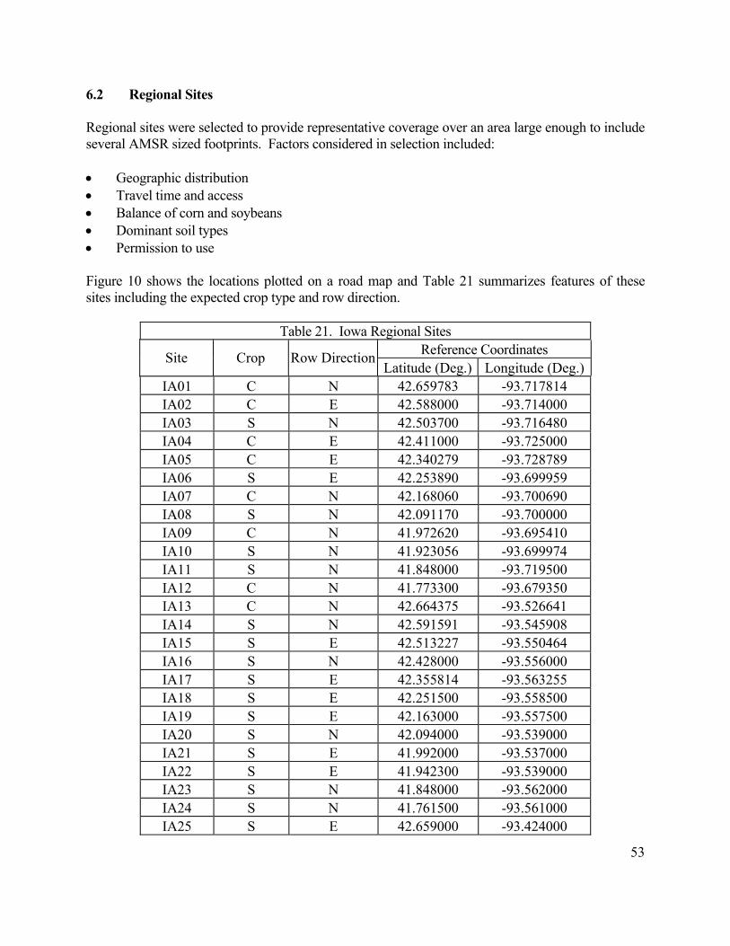
6.2 Regional Sites Regional sites were selected to provide representative coverage over an area large enough to include several AMSR sized footprints. Factors considered in selection included: • Geographic distribution • Travel time and access • Balance of corn and soybeans • Dominant soil types • Permission to use Figure 10 shows the locations plotted on a road map and Table 21 summarizes features of these sites including the expected crop type and row direction.

Table 21. Iowa Regional Sites

Reference Coordinates Site Crop Row DirectionLatitude (Deg.) Longitude (Deg.)

IA01 C N 42.659783 -93.717814 IA02 C E 42.588000 -93.714000 IA03 S N 42.503700 -93.716480 IA04 C E 42.411000 -93.725000 IA05 C E 42.340279 -93.728789 IA06 S E 42.253890 -93.699959 IA07 C N 42.168060 -93.700690 IA08 S N 42.091170 -93.700000 IA09 C N 41.972620 -93.695410 IA10 S N 41.923056 -93.699974 IA11 S N 41.848000 -93.719500 IA12 C N 41.773300 -93.679350 IA13 C N 42.664375 -93.526641 IA14 S N 42.591591 -93.545908 IA15 S E 42.513227 -93.550464 IA16 S N 42.428000 -93.556000 IA17 S E 42.355814 -93.563255 IA18 S E 42.251500 -93.558500 IA19 S E 42.163000 -93.557500 IA20 S N 42.094000 -93.539000 IA21 S E 41.992000 -93.537000 IA22 S E 41.942300 -93.539000 IA23 S N 41.848000 -93.562000 IA24 S N 41.761500 -93.561000 IA25 S E 42.659000 -93.424000

53

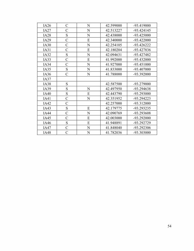
IA26 C N 42.599000 -93.419000 IA27 C N 42.513227 -93.424145 IA28 S N 42.438000 -93.425000 IA29 C E 42.340000 -93.422000 IA30 C N 42.254105 -93.426222 IA31 C E 42.180204 -93.427836 IA32 S N 42.094631 -93.427482 IA33 C E 41.992000 -93.432000 IA34 C N 41.927000 -93.451000 IA35 S N 41.833000 -93.407000 IA36 C N 41.788000 -93.392000 IA37 IA38 S 42.587500 -93.279000 IA39 S N 42.497950 -93.294638 IA40 S E 42.443790 -93.293000 IA41 C N 42.351952 -93.294223 IA42 C 42.257000 -93.312000 IA43 S E 42.179775 -93.293235 IA44 C N 42.090769 -93.293608 IA45 C E 42.003000 -93.292000 IA46 S E 41.948891 -93.292729 IA47 C N 41.848040 -93.292306 IA48 C N 41.782036 -93.303000

54

7 SCHEDULE Table 22. SMEX02 Schedule

9-Jun 10 11 12 13 14 1

Surface Flux/Lidar AH 8:00 am Setup Setup Setup

Ground Soil Moisture

C-130

P3-B Return Installation Installation Installation Installation

DC-8

Twin Otter

USU Arrive Test Flights

Satellite Data Sets L5 L7, AVegetation Set 1 Set 1 Set 1 Set 1

16 17 18 19 20 21 22

Surface Flux/Lidar

Ground Soil Moisture

C-130 Arrive

P3-B Installation Installation Installation Check Installation Check Flight Installation

DC-8

Twin Otter Arrive Test Flights

USU

Satellite Data Sets L7, AVegetation Set 1 Set 1 Set 1

23 24 25 26 27 28 29

Surface Flux/Lidar

Ground Soil Moisture AH 8:00 am

C-130 AH 4:00 pmP3-B AH 4:00 pm

DC-8

Twin Otter AH 4:00 pm

USU Depart AH 4:00 pm

Satellite Data Sets L5 ESVegetation AH 1:00 pm Set 2 Set 2 Set 2

30 1-Jul 2 3 4 5 6

Surface Flux/Lidar

Ground Soil Moisture

C-130

P3-B

DC-8 Arrive

Twin Otter

USU Arrive

Satellite Data Sets L5 L7, A ES ES E2 ESVegetation Set 2 Set 2 Set 2 Set 3 Set 3 Set 3 Set 3

7 8 9 10 11 12

Surface Flux/Lidar

Ground Soil Moisture

C-130 Depart

P3-B Depart

DC-8 Depart

Twin Otter

USU

Satellite Data Sets L7, A, ES L5, ES

Vegetation Set 3 Set 3 Set 3 Set 3

5

13

55

8 GROUND BASED OBSERVATIONS 8.1 Tower-based Flux Measurements Through this project and collaborative relationships we will deploy a number of eddy covariance systems through the study area, with each system consisting primarily of Campbell Scientific CSAT3 3-D sonic anemometer and KH20 krypton hygrometer, measuring momentum flux and sensible and latent heat fluxes between the land and the atmosphere across the watershed. Figure 20 illustrates a typical tower installation. These observations will be representative at the “patch” or local scale (i.e., length scales ~ 102 m). Investigators from USDA-ARS, Utah State University, University of Virginia, University of Iowa, and Texas A&M will be involved. These systems will also have a picture of the complete energy balance by including net radiation, soil heat flux, and radiometric surface temperature measurements. There is also an effort planned by NSTL and Iowa State University scientists to make detailed soil heat flux measurements at several locations within the watershed at varying landscape positions to assess within canopy scale variability. In addition, there will be several systems, which will also be measuring net carbon exchange by eddy covariance with the 3D sonic and LiCor LI-7500 open path CO2/H20 sensors. This will permit a very detailed assessment of water-energy-carbon fluxes and controls as a function of crop type and amount of cover and tillage practices. For selected sites with a significant fractional bare soil component, there are also plans to make measurements of soil respiration using LiCor LI-6200 sensors. Details on the flux tower measurements are provided in Chapter 10.

Figure 20. Typical surface flux tower.

56

8.2 Lidar/Sodar/Radisonde Measurements

Several ground-based atmospheric sensing systems are proposed for deployment for investigating the role of land surface heterogeneity on atmospheric properties and processes. The Raman scanning Lidar from Los Alamos National Lab (LANL) will provide water vapor concentration fields in the lower boundary layer, and a scanning wind Lidar from the University of Iowa (UI) will provide horizontal winds throughout the boundary layer. A scanning elastic Lidar also from UI will map winds in the area, boundary layer height, entrainment zone properties and cloud information. A sodar and radar/RASS system from LANL will be used to measure meso-synoptic scale atmospheric conditions. The Lidar measurements will be coordinated with tower-based flux measurements conducted over several fields having significant differences in roughness and and/or fractional vegetative cover due to differences in planting dates and/or planting method (i.e., drilled versus row planting). The Lidar data provide distributed water vapor and wind fields over the mapped surface temperature, moisture, and cover data. This would be the first time that such detailed data are collected simultaneously, and will provide the basis for assessing the injection of spatial heterogeneity form the land surface and into the lower atmosphere. Radiosondes are a key element in upper air observation systems. Balloon-borne radiosondes measure upper air temperature, humidity and pressure during their ascent to the upper atmosphere. Radiosonde signals are received and processed by ground equipment, which automatically computes wind speed and direction using global navigation networks. 8.3 Sun Photometer The NASA Aeronet, which is led by Brent Holben, will provide SMEX02 with an eight channel (Cimel) sun photometer. The sun photometer is designed to view the sun and sky at preprogrammed intervals for the retrieval of aerosol optical thickness and water vapor amounts, particle size distribution, aerosol scattering, phase function, and single scattering albedo. It measures the intensity of sunlight arriving directly from the Sun. Although some Sun photometers respond to a wide range of colors or wavelengths of sunlight, most include special filters that admit only a very narrow band of wavelengths. These measurements are used to radiometrically correct satellite imagery in the visible and infrared bands. By radiometrically correcting these images it is then possible to quantitatively extract physical parameters and compare multiple dates. The instrument will be installed at a central location to provide data appropriate for the intensive site and for the regional area studies. 8.4 Vegetation and Land Cover Vegetation biomass and soil moisture sampling will be performed for all watershed (WC) sites. The measurements that will be made are:

• Plant height • Ground cover • Stand density

57

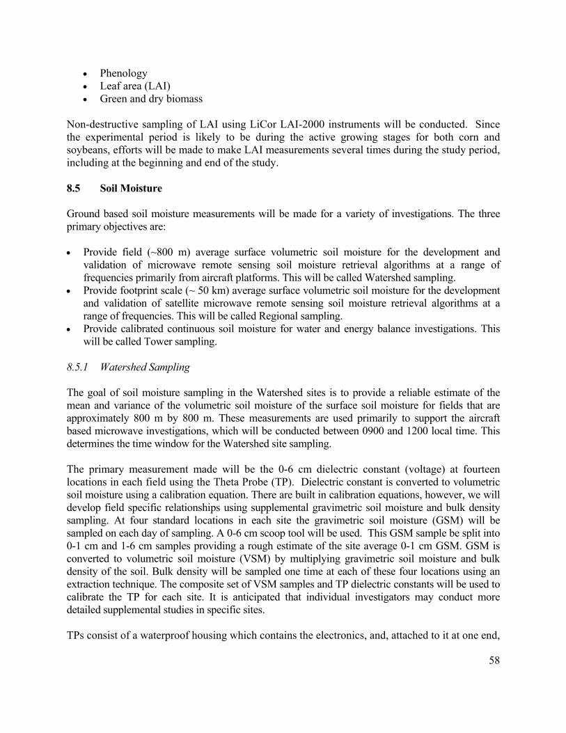
• Phenology • Leaf area (LAI) • Green and dry biomass

Non-destructive sampling of LAI using LiCor LAI-2000 instruments will be conducted. Since the experimental period is likely to be during the active growing stages for both corn and soybeans, efforts will be made to make LAI measurements several times during the study period, including at the beginning and end of the study. 8.5 Soil Moisture Ground based soil moisture measurements will be made for a variety of investigations. The three primary objectives are: • Provide field (~800 m) average surface volumetric soil moisture for the development and

validation of microwave remote sensing soil moisture retrieval algorithms at a range of frequencies primarily from aircraft platforms. This will be called Watershed sampling.

• Provide footprint scale (~ 50 km) average surface volumetric soil moisture for the development and validation of satellite microwave remote sensing soil moisture retrieval algorithms at a range of frequencies. This will be called Regional sampling.

• Provide calibrated continuous soil moisture for water and energy balance investigations. This will be called Tower sampling.

8.5.1 Watershed Sampling The goal of soil moisture sampling in the Watershed sites is to provide a reliable estimate of the mean and variance of the volumetric soil moisture of the surface soil moisture for fields that are approximately 800 m by 800 m. These measurements are used primarily to support the aircraft based microwave investigations, which will be conducted between 0900 and 1200 local time. This determines the time window for the Watershed site sampling. The primary measurement made will be the 0-6 cm dielectric constant (voltage) at fourteen locations in each field using the Theta Probe (TP). Dielectric constant is converted to volumetric soil moisture using a calibration equation. There are built in calibration equations, however, we will develop field specific relationships using supplemental gravimetric soil moisture and bulk density sampling. At four standard locations in each site the gravimetric soil moisture (GSM) will be sampled on each day of sampling. A 0-6 cm scoop tool will be used. This GSM sample be split into 0-1 cm and 1-6 cm samples providing a rough estimate of the site average 0-1 cm GSM. GSM is converted to volumetric soil moisture (VSM) by multiplying gravimetric soil moisture and bulk density of the soil. Bulk density will be sampled one time at each of these four locations using an extraction technique. The composite set of VSM samples and TP dielectric constants will be used to calibrate the TP for each site. It is anticipated that individual investigators may conduct more detailed supplemental studies in specific sites. TPs consist of a waterproof housing which contains the electronics, and, attached to it at one end,

58

four sharpened stainless steel rods that are inserted into the soil. The probe generates a 100 MHz sinusoidal signal, which is applied to a specially designed internal transmission line that extends into the soil by means of the array of four rods. The impedance of this array varies with the impedance of the soil, which has two components - the apparent dielectric constant and the ionic conductivity. Because the dielectric of water (~81) is very much higher than soil (typically 3 to 5) and air (1), the dielectric constant of soil is determined primarily by its water content. The output signal is 0 to1V DC for a range of soil dielectric constant, ε, between 1 and 32, which corresponds to approximately 0.5 m3 m-3 volumetric soil moisture content for mineral soils. More details on the probe are provided in the sampling protocol section of the plan. 8.5.2 Regional Sampling The goal of soil moisture sampling in the Regional sites is to provide a reliable estimate of the VSM mean and variance within a single satellite passive microwave footprint (~50 km) at the nominal time of the Aqua AMSR overpass (1330 local time). The exact center location and orientation of the satellite footprint will vary with each overpass. A grid of 48 individual sites will be sampled each day that covers a domain of approximately 50 km by 100 km (4 by 12 sites). A single location in each of these 48 sites will be sampled. As noted, these measurements are used primarily to support the Aqua AMSR based microwave investigations, therefore, the Regional sampling will be conducted between 1200 and 1500 local time. The primary measurement made will be the 0-6 cm dielectric constant at a single location in each site using the Theta Probes described above Dielectric constant is converted to volumetric soil moisture using a calibration equation. There are built in calibration equations, however, we will develop field specific relationships using supplemental gravimetric soil moisture and bulk density sampling. A different approach will be used for the Regional sites than the Watershed sites. Each sampling day, a coring tool will be used to extract a single VSM sample of the 0-1 cm and 1-6 cm soil layers. The composite set of VSM samples and TP dielectric constants will be used to calibrate the TP for each site. It is anticipated that individual investigators may conduct more detailed supplemental studies in specific sites. 8.5.3 Tower Sampling Tower sampling is intended to provide continuous measurements of the surface soil moisture at the locations of the surface flux towers. A single Vitel Hydra capacitance sensor will be installed at a depth of 5 cm. To insure accurate calibration of these devices, the TP and GSM measurements will be made near these locations on each sampling date. This effort will include the SCAN site. Each surface flux tower will include instruments to measure the surface layer soil moisture and temperature and the surface temperature. This will be a continuous record at a single point within the field site. Cross referencing to the watershed site sampling will be done by collecting Theta Probe soil moisture, gravimetric soil moisture, soil temperature and surface temperature at a location in the vicinity of the tower each time sampling is conducted.

59

Soil moisture and temperature for the surface layer will be measured using Vitel Type A Hydra Probes. This version is compatible with Campbell CR-10 data loggers, the temperature output voltage never exceeds 2.5 volts. The Hydra Probe (HP) soil moisture probe determines soil moisture and salinity by making a high frequency (50 MHz) complex dielectric constant measurement. A complex dielectric constant measurement resolves simultaneously the capacitive and conductive parts of a soil's electrical response. The capacitive part of the response is most indicative of soil moisture while the conductive part reflects predominantly soil salinity. Temperature is determined from a calibrated thermistor incorporated into the probe head. As a soil is wetted, the low dielectric constant component, air, is replaced by water with its much higher dielectric constant. Thus as a soil is wetted, the capacitive response (which depends upon the real dielectric constant) increases steadily. Through the use of appropriate calibration curves, the dielectric constant measurement can be directly related to soil moisture. The dielectric constant of moist soil has a small, but significant, dependence on soil temperature. The soil temperature measurement that the Hydra probe makes can be used to remove most of the temperature effects. The Hydra probe has three main structural components, a multiconductor cable, a probe head, and probe sensing tines. The probes will be installed horizontally in the soil with the center tine at a depth of 5 cm. Additional details on the Hydra probe are provided in the sampling protocol section of this plan. The measured raw electrical parameters determined by the HP are the real and imaginary dielectric constants. These two parameters serve to fully characterize the electrical response of the soil (at the frequency of operation, 50 MHz). These are both dimensionless quantities.

Because both the real and imaginary dielectric constants will vary somewhat with temperature, a temperature correction using the measured soil temperature is applied to produce temperature corrected values for the real and imaginary dielectric constant. The temperature correction amounts to calculating what the dielectric constants should be at 25oC.

The dielectric constants are used to calculate soil moisture with conversion equations. The manufacturer provides these, however, through the ground sampling component it should be possible to refine these for each site. 8.6 Soil and Surface Temperature

The objectives of the soil and surface temperature are nearly identical to those of soil moisture. There are a few differences related to the spatial and temporal variability of temperature versus soil moisture. Typically the soil temperature exhibits lower spatial variability, especially at depth. On the other hand surface temperature can change rapidly with changes in radiation associated with clouds. In addition, it can be difficult to correctly characterize surface temperature at satellite

60

footprint scales (30 m – 1 km) using high resolution ground instruments. This is especially true when there is partial canopy cover. The surface temperature will be sampled using handheld infrared thermometers (IRT). The soil temperatures will be obtained using a temperature probe inserted to depths of 1 cm, 5 cm, and 10 cm depths. 8.6.1 Watershed Sampling Temperature sampling will be conducted at the four locations selected for GSM sampling. These will be distributed over the each site. 8.6.2 Regional Sampling Temperature sampling will be conducted at the specific single location selected for sampling in the site. 8.6.3 Tower Sampling Tower sampling is intended to provide continuous measurements of the surface temperature and 2.5 cm soil temperature at the locations of the surface flux towers. The Vitel HP sensor also provides temperature at 5 cm. An Apogee infrared sensor will be installed on each tower and will provide surface observations. This device provides the measured surface temperature and the sensor housing temperature. This second observation can be used to adjust for diurnal effects. These will be installed at a height of 2 m on the tower at an angle of 30 degrees. More information can be found in the protocols section of the plan. When GSM is sampled at the towers the surface and soil temperatures will also be sampled. This effort will include the SCAN site. The temperature measurement provided by the Hydra probe is in degrees Celsius. 8.7 Surface Roughness Each Watershed site will be characterized one time during the time frame. The grid board photography method employed in previous experiments will be used. 8.8 Ground Based Microwave Radiometer The University of Tokyo in cooperation with the Japanese ADEOS-II AMSR program will deploy a ground based microwave radiometer (GBMR) at a site in the Iowa study area. This will most likely be in the watershed. A version of this instrument was part of SGP99. Table 23 describes the basic parameters of the GBMR and Figure 21 shows the likely instrument configuration for SMEX02. The observation strategy is to leave the GBMR at a single location for the duration of SMEX02 and collect diurnal data over several adjacent fields (or plots). This location will likely be at the

61

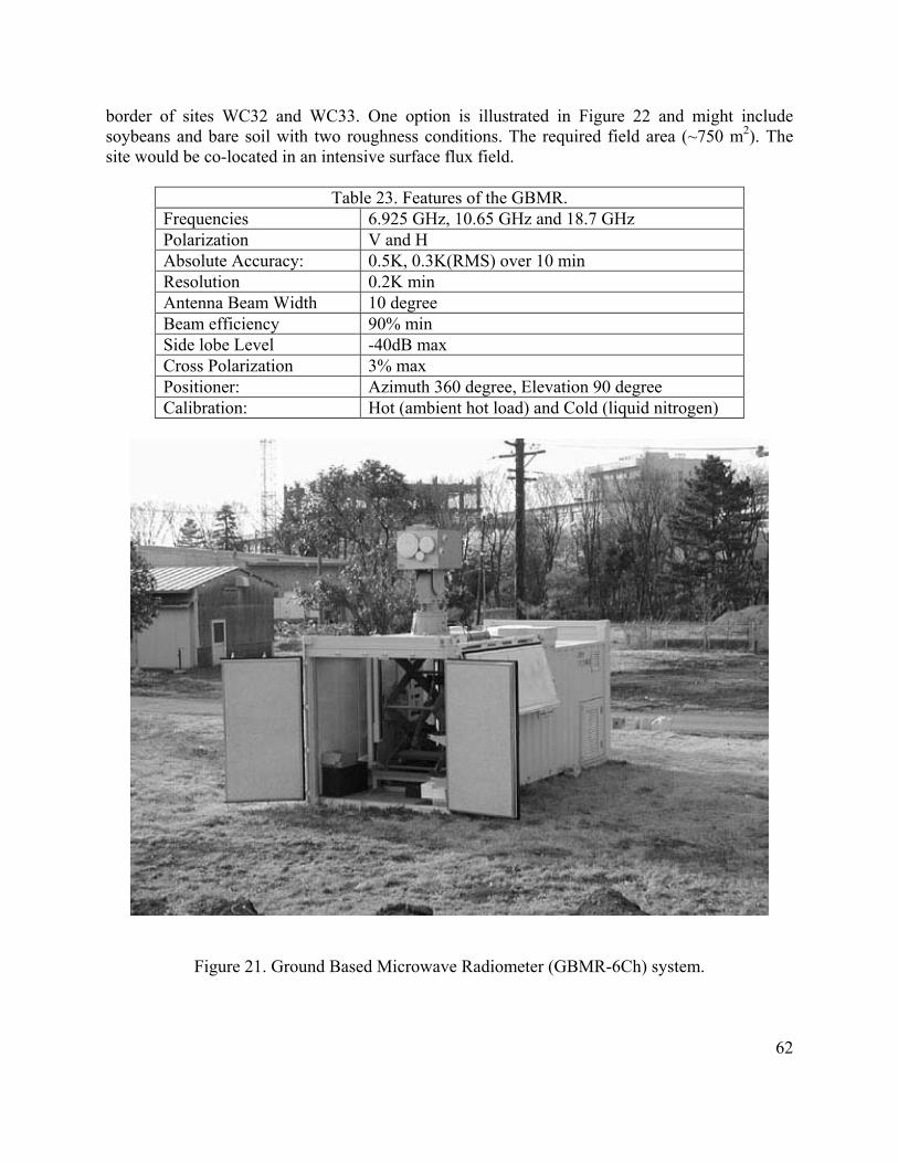
border of sites WC32 and WC33. One option is illustrated in Figure 22 and might include soybeans and bare soil with two roughness conditions. The required field area (~750 m2). The site would be co-located in an intensive surface flux field.

Table 23. Features of the GBMR. Frequencies 6.925 GHz, 10.65 GHz and 18.7 GHz Polarization V and H Absolute Accuracy: 0.5K, 0.3K(RMS) over 10 min Resolution 0.2K min Antenna Beam Width 10 degree Beam efficiency 90% min Side lobe Level -40dB max Cross Polarization 3% max Positioner: Azimuth 360 degree, Elevation 90 degree Calibration: Hot (ambient hot load) and Cold (liquid nitrogen)

Figure 21. Ground Based Microwave Radiometer (GBMR-6Ch) system.

62

In addition to the microwave observations, this group will also collect the following observations:

Surface and 2.5 cm soil/vegetation temperature • • • • • •

Soil moisture at 1 cm, 2.5 cm and 5 cm. Diurnal cycles: 2 hours interval operation for 24 hours for all footprints Vegetation sampling Roughness and bulk density: one sample per day at one location near footprint. Atmospheric forcing data collection (Downward shortwave radiation, Downward longwave radiation, Relative humidity (Reference height), Air temperature (Reference height), Wind velocity (Reference height), and Precipitation)

AWS

Vegetation

GB

Figure 22 Ground Based Micro

30m

MR-6Ch

~13.5m

Note: Clear Sur

Roughness Study

Bare soil:

wave Radiometer (GBMR-6C

~2.5m

rounding

h) footprints

25m

θ =65

=55θ

63

9 REGIONAL NETWORKS AND GENERAL SITE CONDITIONS 9.1 USDA Soil Climate Analysis Network (SCAN) The USDA NRCS has initiated nationwide soil moisture and soil temperature (SMST) analysis network called SCAN. Details and data can be obtained at the following web site http://www.wcc.nrcs.usda.gov/smst/smst.html. Hourly observations are provided to the public on the Internet in real time. Each system provides hourly observations of: Air temperature Barometric pressure Wind speed Precipitation Relative humidity Solar radiation Soil temperature at 5, 10, 20, 50 and 100 cm Soil moisture at 5, 10, 20, 50 and 100 cm A SCAN site was installed near Ames, IA at Latitude: 42.00o, Longitude: 93.74o and Elevation: 1073 Feet on 09/23/2001. Figure 23shows the site conditions.

Figure 23 SCAN site at Story County, IA

64

9.2 NSTL Meteorological Stations NSTL operates rain gages, stream gages, and meteorological stations within the Walnut Creek watershed. All are on data loggers, which are downloaded on a weekly basis. The locations of these are shown in Figure 24 Data for the SMEX02 time period will be provided following the experiment. Other periods of record may be obtained by contacting NSTL.

Figure 24 Rain rages (stars) and steam gages (flags) within the Walnut Creek watershed. Other meteorological stations are indicated as triangles. The large yellow box is 2 km by 2 km and is used to represent scale. Two of the rain gage sites include additional meteorological observations (701 and 702). Measurements are made every minute and recorded every hour. End of day max-min air temp and daily total rainfall and max wind speed are recorded. Observations made are: • solar radiation (kJ/m2) • air temperature (C) • saturated vapor pressure (kPa) • actual vapor pressure (kPa) • 4 cm soil temperature (C) • 20 cm soil temperature (C) • wind speed (m/s) • wind direction (degrees) • hourly total rainfall (mm)

65

9.3 Iowa Environmental Mesonet The Iowa Environmental Mesonet (IEM) collects environmental data from cooperating members with observing networks. The data is stored and available on the following website. http://mesonet.agron.iastate.edu/. Contributors are Iowa State University, the National Weather Service, the Iowa Department of Transportation and local sponsored school networks. Nearby station locations in the Iowa State Agroclimate portion of the network are shown in Figure 24 Iowa State AgClimate stations provide measurements of Precipitation Inches Solar Radiation Kilo calories per meter squared Air Temperature Fahrenheit Soil Temperature (10 cm) Fahrenheit Wind speed MPH Wind Direction Degrees Relative Humidity % Time local time, either CST or CDT These data are available as real time plots or can be extracted from archives. The NWS operates three networks of interest. Automated Surface Observing System (ASOS). Stations are located at airports and measurements are made every minute of temperature, dew point, wind, altimeter setting, visibility, sky condition, and precipitation. They also operate the Automated Weather Observing System (AWOS), which provides wind speed and direction, temperature and dew point, visibility, cloud heights and types, precipitation, and barometric pressure. Finally, limited observations of precipitation and temperature are available through the NWS Cooperative Observer Program [COOP] in which daily observations are reported by volunteer observers.

66

10 SMEX02/SMACEX TOWER FLUX MEASUREMENTS 10.1 Eddy Covariance Measurements The tower flux team is composed of individuals from eight (8) locations. The primary participants include; John Albertson (Duke Univ.), Tony Cahill (Texas A&M), Dan Cooper (Los Alamos National Lab), Bill Eichinger (Univ. of Iowa), Larry Hipps (Utah State Univ.), Bill Kustas (USDA-ARS-HRSL), John Norman (Univ. of Wisconsin) and John Prueger/Jerry Hatfield (USDA-ARS-NSTL). Instruments The instruments that are being in used in the study are provided by these individuals and are listed in Table 21. At present fifteen (15) CSAT3 sensors (Campbell Scientific 3-D sonic anemometer) and eleven (11) LI7500 (Li-Cor CO2/H2O analyzer) are available. This will give the ability to mount 11 eddy covariance (EC) systems in the study that will provide us with time series (high frequency) data of wind (u, v, and w components), sonic temperature (TS), air temperature (TA) if a fine wire thermocouple is mounted with the CSAT3, water vapor and CO2 from the LI7500. The remaining 4 CSAT3 will be used with KH20 sensors (Campbell Scientific 1-D Krypton Hygrometers/ H2O sensors) to provide the same data as above except for CO2. With one CSAT3/KH20 system reserved as backup, a total of 14 EC systems will in operation during the study. Logging Measurements Each of the EC systems will have a Campbell 23X data logger to execute the time series commands. Twelve (12) of the EC systems will have a Libretto (Toshiba) 30, 50 or 70 mini computer to store all the raw high frequency data in “time series mode”. Each mini computer will have a PCMCIA card of either 80 or 128 Mb storage capacity. In short, the mini computers will be communicating with the 23X grabbing the data from the 23X and storing it onto the PCMCIA cards. Approximately every 24 hours, and most likely at the beginning of each day, the PCMCIA cards will be exchanged at each EC tower with new PCMCIA cards. During this time input location channels of the EC components will be viewed online and inspected for instrument performance and instantaneous data integrity. If the EC systems are performing without error, normal time series acquisition will be resumed with no loss of data. If a problem is encountered, it will be solved, noted in field logbooks and data acquisition resumed. The 2 remaining EC systems will be running in “flux mode” with 10-minute output of the fluxes being stored on the 23X. Note: Laboratory EC tests at the NSTL during the month of February and March 2002 have found that the high frequency (20 Hz) data acquisition works best with only the CSAT + LI7500 or CSAT + KH20. Attempts have been made to include radiometric measurements with the Apogee IRT in the EC data stream. The results have consistently been loss of data in the 20 Hz stream. No loss of data has occurred with doing only the EC instruments. Therefore, radiometric

67

temperature and all other non-EC measurements will be recorded separately on a 21X data logger. Table 24 lists the inventory of eddy covariance/ancillary measurement instrumentation committed by the various investigators.

Table 24 List of Instrumentation Supplied by Investigators for the Flux Tower Observations. INVESTIGATOR

CSAT3

LI 7500

KH 20

23X 21X AM25T

NR Lite

CNR 1

IRTS-P

HFT LIBRETTO

3 m Tower

Solar Panels

PCMCIA

NSTL 2 4 8 7 12 1 15 20 13 10 12 -

MSX 60 8-80 mb, 12-128 mb

W. Kustas 2 2 2 4 1 1 4 8 12-128 mb W. Eichenger 3 2 1 4 3 T. Cahill 2 1 2 4 2 6 12 1 2 - 40W L. Hipps 2 2 2 2 1- 75W J. Albertson 2 2 2 4 2 5 8 4 - 40W J. Norman 1 D. Cooper 1 7

TOTALS 15 11 10 15 12 12 3 7 30 52 14 20 19 32

As a reminder the NSTL will provide two deep cycle batteries per site as well as Libretto computers and customized enclosures for the 23x. s it stands now (April. 05, 2002) we can field 14 eddy covariance systems (11 w/ LI 7500 and 3 w/ KH20) for 20 Hz data acquisition. Important points to keep in mind; There will be two inter-comparisons of eddy covariance and net radiation instrumentation, one in May, and one at the end of the experiment (July). The inter-comparison will be in flux mode 20-30 minute average LE, H, CO2 and Rn. Results of the first inter-comparison will be quickly distributed among the investigators (as in days after the inter-comparison) for investigator review. We will need all the instrumentation in the above Table at the NSTL by the end of April for instrument check out and fitting to the enclosures. The NSTL will be keeping meticulous notes of serial numbers of instrumentation/owners. When you send in your instruments we will be sending a verification list of what the NSTL received as soon as we receive the instrumentation. The NSTL has just purchased a dedicated computer to archive all of the flux data. 2.0 GHz Pentium III 512 mb RAM, 80 G HD, double PCMCIA card reader, CD-RW, DVD etc…the idea is simple, PCMCIA cards will be exchanged every morning at all sites following daily sensor check. PCMCIA cards will be brought to the NSTL. NSTL techs will transfer data from the PMCIA cards to the computer, (the data will be in binary form), techs. will convert binary to ASCII and perform the 2 scan offset correction for T, CO2, and H2O signals (sync up with the CSAT data) and then package the data into convenient 1 hr blocks of 20 Hz ASCII data. This process will complete the archive process and will take place daily. After the archive process the techs will run a Mathematica notebook to compute 30 minute fluxes from the 20 Hz data, (this 68

will include Webb-Pearman-Leuning corrections so that investigators will be able to look at the data within a few hours after it has been archived. As the end of the experiment comes to a close, all archived data will be burned onto DVD's. Sampling Frequency and Output Averages EC systems (CSAT3 with either LI7500 or KH20) will be sampled at 20 Hz. For 12 of the 14 EC systems no averaging of output will be performed with the data recorded in binary. The remaining 2 EC systems will have 10-min averages recorded. 10.2 Ancillary Measurements Ancillary measurements will include the remaining energy balance components, namely net radiation (RN), and soil surface heat flux (GS) which includes soil heat flux across the heat flow transducer (G), and heat transfer of the soil layer above the transducers, the storage term (S), so that GS=G+S. The magnitude of S is dependent on soil heat capacity, which is a function of soil texture and soil moisture, and the temporal trace of soil temperature (TSOIL). The most accurate estimate of S will be obtained when the data is post-processed, however, nominal values of S could be computed and stored in the output files using the existing NSTL soil texture database for the field sites. Radiometric temperature observations of the soil-vegetation canopy system or composite surface temperature, (TRAD,C) and one of the bare soil surface (TRAD,S), will be made at each site. Mean air temperature (TA) and relative humidity (RH) and soil moisture (W) using a heat capacity probe. Depending on availability, measurements of mean wind speed (cup anemometer), wind direction (wind vane) and total precipitation (tipping bucket rain gage) may also be made at some of the sites. Instruments Net radiation will be made using primarily one of three RN sensors, the Kipp&Zonen CNR1 or NR Lite and the Radiation and Energy Balance (REBS) Q*7 series. There are seven (7) CNR1 and three (3) NR Lite sensors, requiring the remaining four (4) sites to be instrumented with REBS Q*7 series sensors. Since there are issues associated with instrument response and differing sensitivity to long and short wave radiation among RN sensors, we will conduct an inter-comparison among the sensors at the beginning and end of the study and evaluate differences. In addition we will assign priority levels to the flux sites so as to insure that the highest priority sites receive the “A” suite of instruments, i.e. the CSAT3 with LI7500 and a CNR1 net radiometer. For the sites having the CNR1 net radiometer, all four-radiation components will be recorded, namely incoming and outgoing short and long wave radiation. Soil flux G will be measured using REBS HFT3 soil heat flow transducers (plates) and the soil temperature measurements of the soil layer above the HFT3 sensors for estimating S will be made using type-T soil thermocouples manufactured by NSTL. The TRAD,C and TRAD,S observations will be made using Apogee precision radiometers (model IRTS-P). Mean TA and RH will be made using Vaisala temperature/RH probe (model HMP45C) enclosed in a radiation shield. Values of W will be estimated using the Vitel Hydra (Model type A) soil heat capacity probe.

69

Logging Measurements For the 12 sites in “time series mode”, ancillary measurements will be made using a Campbell 21X data logger connected to a Campbell AM 25T multiplexer (see Table 24). The two remaining sites running in “flux mode” will have an additional 23X to collect the ancillary measurements. Sampling Frequency and Output Averages: The TRAD and RN measurements will be sampled at 1 Hz or 1-sec with 60 seconds or 1-min average output. TA, RH, G, and TSOIL will be sampled every 0.1 Hz or 10-sec with a 10-min average output. 10.3 Intercomparison Two intercomparisons are planned for study, one before the experiment and one after. The intercomparisons will include eddy covariance instruments, net radiation, and IRTs. The purpose of the intercomparison will be to assess measurement difference and variance when made over a uniform surface. This will provide guidance when determining if, for example, a 25-50 W m-2 difference in turbulent heat flux or net radiation between two or more sites is greater than the uncertainty in the measurements. We need to establish confidence limits in our measurements. Two intercomparisons are planned because of the significant vegetative differences the fields will undergo during the course of this study. 10.4 Instrument Height/Depth And Position See Table 22 for a summary of the measurement height/depth of the sensors. Eddy Covariance Sensors Triangular towers (radio towers) will be used to mount the EC sensors and instrumentation for the ancillary measurements. A 6 meter tower (combining two 3-m triangular tower sections) anchored by 3 guy wires will be placed in the corn field sites while a single 3-m triangular tower section will be used for the soybean field sites. For the soybean crop, the vegetation height is not expected to exceed ~0.5-1 m by the end of the experimental period in mid-July. The corn crop, however, may be significantly taller since this season, an earlier than normal planting date (mid-April) is being scheduled due to relatively dry winter and early warm spring conditions. Depending on rainfall amounts after planting and degree-days, the corn height could be greater than 1 m by mid-June and reach ~2-3 m by the end of the experiment in mid-July. To maintain an acceptable measurement height above the canopy for the EC sensors and at the same time remain within the upwind source-area or fetch of the individual field sites, we propose maintaining a ~1.5 m height above the corn and soybean canopies during the experimental period. Given the measurement configuration for the two tower heights, and typical size of the fields (~400 x 400 m) this is a reasonable compromise for both corn and soybean canopies.

70

The NSTL will provide ten (10) 3-m sections of radio tower while Los Alamos and University of Iowa can provide seven (7) and three (3) 3-m sections of radio tower, respectively (see Table 25). With a total of twenty (20) 3-m sections we can have at a minimum six (6) EC systems in corn on 6-m radio towers. This will permit the corn canopy to reach its maximum height of ~3 m during the study, and still maintain EC sensors at 1.5 m above the canopy. This leaves us with eight (8) 3-m radio tower sections for use in the soybean field sites. The 3-m towers will be sufficiently tall for the soybean crop since the maximum height by mid-July would be ~1 m. Soybeans could reach a canopy height of ~1.5 m, but only under extraordinary conditions and this height wouldn’t be attained until later in August. Since the predominant wind directions in the summer growing season are from the south and southwest, the EC sensors will be pointing south.

Table 25. A summary of sensor height/depth for the flux towers in the corn and soybean field sites

Sensor/Instrument Sensor Height/Depth for Corn

Sensor Height/Depth for Soybean

EC System/CSAT3-LI7500 or KH20 ~2 to 4.5 m AGL* ~1.5 to 2 m AGL* Net Radiometer/CNR1, NR-Lite, Q*7 ~6 m AGL ~3 m AGL

Surface Temperature/IRTS-P ~6 m and ~0.4 m AGL@ ~3 m and ~0.4 to 0.1 m AGL@

Air Temperature-Relative Humidity/HMP-45C

~2 to 4.5 m AGL* ~1.5 to 2 m AGL*

Soil Heat Flux Plate/HFT -0.06 m -0.06 m Soil Temperature/Type-T Thermocouple -0.02 and –0.04 m -0.02 and –0.04 m

Soil Moisture/Hydra Type A -0.05 m# -0.05 m# *The EC and air temperature/relative humidity sensors will be moved to maintain ~1.5 m height above the crop. @There will be two (2) IRT sensors, one nadir viewing from the top of the tower and the other within the canopy at ~45 degree viewing angle measuring soil surface temperature at a height primarily as a function of row spacing. #The soil moisture sensor will have the center of the sensor at -0.05 cm so that the sensor is effectively sampling a bulk near-surface (~0-0.07 m) soil moisture.

Ancillary Instrumentation Net Radiation: Net radiation instruments will be mounted at the top of the radio towers oriented to the south at a fixed height near or at the top of the radio towers, specifically at ~6 m and 3 m above ground level (AGL). They will be positioned further away (south) from the tower than the EC system positioned below, to avoid instrument shadowing and influences of EC sensors on reflected/upwelling radiance measurements. Radiometric Surface Temperature: The two Apogee IRT sensors will be positioned at two heights and viewing angles. The sensor for measuring a composite temperature, TRAD,C will be positioned at the top of the tower with a nadir viewing angle. The IRTS-P model has a nominally 3:1 field of view (FOV) so that at 3 m AGL the FOV is a 1 m diameter circle. To minimize any contamination from the tower and instrumentation, the nadir-viewing IRT will be 71

positioned on the east side of the tower and located ~2 m away from the tower. The other IRTS-P for estimating TRAD,S will be placed in the center of the row crop on a short pole with a measurement height of ~ 0.1 to 0.4 m AGL and nominally a 45 degree view angle from nadir. The sensor will view the soil surface parallel to the row direction (either north-south or east-west) to obtain a spatial representation of the average bare surface soil temperature. The actual TRAD,S measurement height will depend primarily on crop row spacing with ~ 0.4 m height for the 30-in row crops, and ~0.1 m height for the 8-in row crops. Air Temperature/Relative Humidity: The air temperature/relative humidity sensor will be positioned on the north facing side of the tower at the same height as the EC sensors or ~1.5 m above the canopy. Therefore, it will be repositioned each time the EC sensors are moved. Soil Heat Flux Plates and Soil Thermocouples: Soil heat flux plates will buried at a depth of 0.06 m below the soil surface with Type-T thermocouples at 0.02 and 0.04 m below the soil surface but above the associated soil heat flux plate. Four (4) soil heat flux plates and eight (8) soil temperature sensors will be used for obtaining a spatially-representative value of GS. Each sensor cluster (1 soil heat flux plate and 2 soil temperature sensors) will occupy ¼ of the row, with the cluster placed in the center of each ¼-section. For corn planted in 30-in or ~ 0.76 m row, the ¼-sections will be 0.19 m wide. The row width for soybeans will be vary anywhere from 30-in to 8-in or ~ 0.20 m (drilled soybean) to no real row-structure (flex-coil soybean). For the 0.20 m rows, the ¼-sections will be 0.05 m wide, while for flex-coil soybeans, sensors will need to be placed in a more random fashion. Within the row, the sensor clusters should be placed at different distances from the tower in order to obtain a better spatial sampling of soil and vegetation conditions. In Figure 25, an example of the sampling strategy for a 30-in row crop is illustrated. Soil Moisture Sensor: The soil moisture probe will be buried such that the center of the probe is at 0.05 m depth. This will give a sampling of the near-surface soil moisture condition. The probe will be positioned within the row at a location that approximates a area-weighted sample. For the 30-in (0.76 m) row spacing, the location would be at 0.19 m or ¼ the distance from the row (see Figure 24). 10.5 Selected Flux Sites Twelve (12) of the soil moisture sampling field sites were selected to contain flux towers. Two (2) field sites, one corn and the other soybean, will contain 2 EC systems for investigating within field variability and will also be field sites monitored with the Lidar system. In Table 26 is a listing of the field sites, crop type, row direction, number of EC systems, whether in flux or time series mode, whether using LI7500 or KH20, net radiometer type (i.e., CNR1 or REBS/NR Lite) and Lat/Long location.

72

~76 cm

~19 cm

Row Row

~1-2 m

Figure 25. Schematic (planar view) illustrating sampling design for soil heat flux/soil temperature sensor clusters (solid circles) and location of soil moisture probe (solid square) for a 30-in or 0.76 m row crop. Table 26. Flux tower field sites, cover crop, row direction, number of systems/towers, data collection mode, water vapor and/or CO2 sensor, net radiometer model and reference coordinates.

Field Crop Row Dir.

No. of Towers

Flux (F) or Time Series (T) Mode

LI7500 or KH20

CNR1 or REBS/NR Lite

Latitude (Deg)

Longitude (Deg)

WC03 S N 1 T LI7500 CNR1 41.982193 -93.754082 WC06 C N 1 T LI7500 CNR1 41.933098 -93.746235 WC10 S X 1 F KH20 REBS/NR Lite 41.976228 -93.690514 WC11 C N 1 T LI7500 REBS/NR Lite 41.972237 -93.694506 WC13 S X 1 T LI7500 REBS/NR Lite 41.952925 -93.689670 WC14 S N 1 T KH20 REBS/NR Lite 41.947517 -93.694786 WC15 C E 2 T(2) LI7500(2) CNR1(2) 41.939278 -93.663560 WC16 S E 2 T(2) LI7500(2) CNR1(2) 41.933784 -93.663560 WC23 S E 1 T LI7500 REBS/NR Lite 41.991806 -93.537476 WC24 C N 1 T LI7500 CNR1 41.991806 -93.529163 WC25 S E 1 F KH20 REBS/NR Lite 41.943741 -93.537014 WC33 C E 1 T LI7500 REBS/NR Lite 41.974730 -93.644950

Crop: C=Corn, S=Soybean Row Direction: N=North-South, E=East-West, X=Flex Coil

73

11 SAMPLING PROTOCOLS 11.1 General Guidance on Field Sampling • Sampling is conducted every day. It is canceled by the group leader if it is raining, there are

severe weather warnings or a logistic issue arises. • Know your pace. This helps greatly in locating sample points and gives you something to

do while walking. • If anyone questions your presence, politely answer identifying yourself as a scientist working

on a NASA/USDA soil moisture study with satellites. If you encounter any difficulties just leave and report the problem to the group leader.

• Although gravimetric and vegetation sampling are destructive, try to minimize your impact by filling holes. Leave nothing behind.

• Always sample or move through a field along the row direction to minimize impact on the canopy.

• Please be considerate of the landowners and our hosts. Don’t block roads, gates, and driveways. Keep sites, labs and work areas clean of trash and dirt.

• Watch your driving speed, especially when entering towns. Be courteous on dirt and gravel roads, lower speed=less dust.

• Avoid parking in tall grass, catalytic converters can be a fire hazard. • Close any gate you open as soon as you pass. • Work in teams of two. Carry a cell phone. • Be aware that increased security at government facilities may limit your access. Do not

assume that YOU are exempt. 11.2 Watershed Site Surface Soil Moisture and Temperature Watershed site sampling will take place between 8:30 am and 11:30 am. Soil moisture and temperature sampling of the watershed area sites is intended to estimate the site average and standard deviation. It is assumed here that most of these sites will be quarter sections (800 m by 800 m), however, there will be a number of variations that may require adaptation of the protocol. The variables that will be measured or characterized are: • 0-6 cm soil moisture using the Theta Probe (TP) instrument • 0-1 and 1-6 cm gravimetric soil moistures using the scoop tool • 0-6 cm soil bulk density (separate team) • Surface temperature using a hand held infrared thermometer • 1 cm soil temperature • 2.5 cm soil temperature • 10 cm soil temperature • GPS locations of all sample point locations (one time)

74

Preparation • Arrive at the field headquarters at assigned time. Check in with group leader and review

notice board. • Assemble sampling kit

o Bucket o Theta Probe and data logger (use the same probe each day, it will have an ID) o Scoop tool o 8 cm spatula o 4 cm spatula o Notebook o Pens o Box of cans (see note below) o Soil thermometer o Handheld infrared thermometer o Extra batteries (9v, AA, AAA) o Screwdriver o First aid kit (per car) o Phone (if you have one)

• For the WC sites, each team should take one box of 18 cans. The cans will be numbered XX01-XX18. Use only boxes labeled AA through BZ.

• Verify that your TP, data logger, infrared instrument, and soil thermometer are working. • Check weather • The first time you sample, it will help to use flags to mark your transect rows and sample

point locations. Use only plastic flags and mark with the site ID and point ID (i.e. WC05-02) • All sample points should be located with a GPS once during the experiment. Points will be

referenced by Site “WC##” and Point “##”. • Use a new notebook page each day. Take the time to draw a good map and be legible.

These notebooks belong to the experiment, if you want your own copy make a zerox. Procedure • Upon arrival at a site, note site id (WC##), your name(s) and time in notebook. Draw a

schematic of the field (It might be a good idea to do this before you go out for the day). Indicate the TP ID you are using.

• Assemble 8 sequential cans and indicate on schematic where they will be used. Odd numbered cans are used for the 0 – 1 cm sample and even numbered cans are used for the 1 – 6 cm sample. See Figure 26 as an example of such a diagram.

• Use cans sequentially. • From a reference point for the site (usually a corner), measure 200 m along one side to locate

the first transect. o Transects should be parallel with the row direction. o If possible, select a row that is a tractor row to walk in.

75

• From this location initiate a sampling transect across the site. Take the first sample at 100 m and repeat every 100 m until you are 100 m from the edge of the site. For a standard quarter section site this will result in 7 samples along the transect.

o Sample in the row adjacent to the row you are working in, it is suggested that this be the row to your right.

o At all points collect three TP samples across the row as suggested in Figure 27. See the Theta Probe protocol for how to use the instrument and data logger.

o At points labeled ALL in Figure 26 (four per site) collect One gravimetric soil moisture sample for 0-1 cm and 1-6 cm following the

procedures described using the scoop, enter can numbers on diagram in book (See Gravimetric Sampling with the Scoop Tool protocol)

One soil temperature (Degrees C) for 1 cm, 2.5 cm and 10 cm using the probe, enter values in book (See Temperature Sampling protocol)

One averaged surface thermal infrared temperature (Degrees C) using infrared thermometer, enter value in book (See Temperature Sampling protocol)

• After completing this transect move 400 m perpendicular into the site and initiate a new transect. This will result in a total of 14 sampling points.

o Exit the field before attempting to move to the second transect. • As you move along the transect note any anomalous conditions on the schematic in your

notebook, i.e. standing water. • Record your stop time and place cans in box. Try to keep them cool.

7 6 5 4 3 2 1

8 9 10 11 12 13 14

Start

200 m

100 m

400 m

100 m

Row direction

AllAll

AllAll

7 6 5 4 3 2 1

8 9 10 11 12 13 14

Start

200 m

100 m

400 m

100 m

7 6 5 4 3 2 1

8 9 10 11 12 13 14

Start

200 m

100 m

400 m

100 m

Row direction

AllAll

AllAll

Figure 26. Schematic of layout of samples in a watershed site.

76

Tractor Row

SamplingRow

Theta ProbeSample Points

Tractor Row

SamplingRow

Theta ProbeSample Points

Figure 27. Schematic of layout of Theta Probe sample points.

Sample Data Processing • Return to the field headquarters immediately upon finishing sampling. • For each site, weigh the gravimetric samples and record on the data sheets (Figure 28) that

will be provided. Use a single data sheet for all your samples for that day and record cans sequentially.

• Transfer temperature and other requested data to data sheets (same sheet used for GSM). • Place cans in (in box) “TO OVENS” area and data sheet in collection box. • Turn in your TP and data logger to the person in charge. They will be responsible for

downloading data. • Clean your other equipment.

11.3 Regional Site Surface Soil Moisture and Temperature Regional sampling will take place between 12:00 pm and 3:00 pm. Soil moisture and temperature sampling of the region near Ames Iowa is intended to estimate the site average and standard deviation at the scale of passive microwave satellite footprints and grid cells. The variables that will be measured or characterized are: • 0-6 cm soil moisture using the Theta Probe (TP) instrument • 0-1 and 1-6 cm gravimetric soil moistures and bulk density using the coring tool • Surface temperature using a hand held infrared thermometer • 1 cm soil temperature • 2.5 cm soil temperature • 10 cm soil temperature • GPS locations of all sample point locations (one time)

77

Preparation • Arrive at the field headquarters at assigned time. Check in with group leader and review

notice board. • Assemble sampling kit

o Bucket o Theta Probe and data logger (use the same probe each day, it will have an ID) o Coring tool and coring tool hammer o 8 cm spatula o 4 cm spatula o Funnel o Bottle brush o Notebook o Pens o Box of cans (see note below) o Soil thermometer o Handheld infrared thermometer o Extra batteries o Screwdriver o First aid kit (per car) o Phone

• Verify that your TP, data logger, infrared instrument, and soil thermometer are working. • For the IA sites, each team should take one box of 24 cans. The cans will be numbered

XX01-XX24. Use only boxes labeled CA through CZ. • Check weather • The first time you sample, it will help to use flags to mark the field entry point and sample

point location. Use only plastic flags and mark with the site ID (i.e. IA05) • All sample points should be located with a GPS once during the experiment. Points will be

referenced by Site “IA##”. • Check weather Procedure • Upon arrival at a site, note site id (IA##), your name(s), TP ID, and time in notebook. Draw

a schematic of the field (It might be a good idea to do this before you go out for the day). • Assemble 2 sequential cans. Odd numbered cans are used for the 0 – 1 cm sample and

even numbered cans are used for the 1 – 6 cm sample. • Go to the pre-established sampling location.

o Sample in the row adjacent to the row you are working in, it is suggested that this be the row to your right.

o At the location collect three TP samples across the row as suggested in Figure 27. Always start with the sample directly in the plant row and move out.

o Using the coring tool collect one gravimetric soil moisture sample for 0-1 cm and 1-6 cm following the Coring Tool Sampling protocol, enter can numbers in book

78

o One soil temperature (Degrees C) for 5 cm and 10 cm using the probe, enter values in book

o One averaged surface thermal infrared temperature (Degrees C) using infrared thermometer, enter value in book

o Record your stop time and place cans in box. Try to keep them cool. Sample Data Processing • Return to the field headquarters immediately upon finishing sampling. • Weigh the gravimetric samples and record on the data sheets that will be provided. Use a

separate sheet for each date and record cans sequentially. (see Figure 28) • Transfer temperature and other requested data to data sheets (same sheet used for GSM). • Place cans in “TO OVENS” area and data sheet in collection box. • Turn in your TP and data logger to the person in charge. They will be responsible for

downloading data. • Clean your other equipment. Gravimetric Soil Moisture Sampling Date Observers

Time Sites

Soil Temperature Site ID Sample ID

Wet Weight

Dry Weight

Surface Temperature

1 cm 2.5 cm 10 cm WC01 AB01 210.15 25 22 20 18 WC01 AN02 WC01 AB03 WC01 AB04 WC01 AB05 WC01 AB06 WC01 AB07 WC01 AB08 WC02 AB09

. . WC02 AB16

Figure 28. Example of the gravimetric soil moisture sampling data sheet.

79

11.4 Theta Probe Soil Moisture Sampling and Processing There are two types of TP configurations; Type 1 (Rod) (Figure 29) and Type 2 (Handheld) (Figure 30). They are identical except that Type 1 is permanently attached to the extension rod.

Figure 29. Theta Probe Type 1 (with extension rod).

Figure 30. Theta Probe Type 2. Each unit consists of the probe (ML2x) and the data logger or moisture meter (HH2). The HH2 reads and stores measurements taken with the ThetaProbe (TP) ML2x soil moisture sensors. It can provide milliVolt readings (mV), soil water (m3.m-3), and other measurements. Readings are saved with the time and date of the reading for later collection from a PC. The HH2 is shown in Figure 31. It applies power to the TP and measures the output signal voltage returned. This can be displayed directly, in mV, or converted into other units. It can convert the mV reading into soil moisture units using conversion tables and soil-specific parameters. Tables are installed for Organic and Mineral soils, however, greater accuracy is possible by developing site-specific parameters. For SMEX02, all observations will be recorded as mV and processed later to soil moisture. 80

Use of the TP is very simple - you just push the probe into the soil until the rods are fully covered, then using the HH2 obtain a reading. Some general items on using the probe are: • One person will be the TP coordinator. If you have problems see that person. • A copy of the manual for the TP and the HH2 will be available at the field HQ. They are

also available online as pdf files at http://www.dynamax.com/#6, http://www.delta-t.co.uk and http://www.mluri.sari.ac.uk/thetaprobe/tprobe.pdf..

• Each TP will have an ID, use the same TP in the same sites each day. • The measurement is made in the region of the four rods. • Rods should be straight. • Rods can be replaced. • Rods should be clean. • Be careful of stones or objects that may bend the rods. • Some types of soils can get very hard as they dry. If you encounter a great deal of resistance,

stop using the TP in these fields. Supplemental GSM sampling will be used. • Check that the date and time are correct and that Plot and Sample numbers have been reset

from the previous day. • Disconnect sensor if you see the low battery warning message. • Protect the HH2 from heavy rain or immersion. • The TP is sensitive to the water content of the soil sample held within its array of 4 stainless

steel rods, but this sensitivity is biased towards the central rod and falls off towards the outside of this cylindrical sampling volume. The presence of air pockets around the rods, particularly around the central rod, will reduce the value of soil moisture content measured.

• Do not remove the TP from soil by pulling on the cable. • Do not attempt to straighten the measurement rods while they are still attached to the probe

body. Even a small degree of bending in the rods (>1mm out of parallel), although not enough to affect the inherent TP accuracy, will increase the likelihood of air pockets around the rods during insertion, and so should be avoided. See the TP coordinator for replacement.

Figure 31. HH2 display. 81

Before Taking Readings for the Day Check and configure the HH2 settings

1. Press Esc to wake the HH2. Check Battery Status

2. Press Set to display the Options menu 3. Scroll down to Status using the up and down keys and press Set. 4. The display will show the following

Mem % Batt % Readings #.

• If Mem is not 0% see the TP coordinator. • If Battery is less than 50% see TP coordinator for replacement. The HH2

can take approximately: 6500 TP readings before needing to replace the battery.

• If Readings is not 0 see the TP coordinator 5. Press Esc to return to the start-up screen.

Check Date and Time 6. Press Set to display the Options menu 7. Scroll down to Date and Time using the up and down keys and press Set. 8. Scroll down to Date using the up and down keys and press Set to view. It should be

in MM/DD/YY format. If incorrect see the TP coordinator or manual. 9. Press Esc to return to the start-up screen. 10. Press Set to display the Options menu 11. Scroll down to Date and Time using the up and down keys and press Set. 12. Scroll down to Time using the up and down keys and press Set to view. It should be

local (24 hour) time. If incorrect see the TP coordinator or manual. 13. Press Esc to return to the start-up screen.

Set First Plot and Sample ID 14. Press Set at the start up screen to display the Options Menu. 15. Scroll down to Data using the up and down keys and press Set. 16. Select Plot ID and press Set to display the Plot ID options. 17. The default ID should be A. If incorrect scroll through the options, from A to Z, using

the up and down keys, and press Set to select one. 18. Press Esc to return to the main Options menu. 19. Scroll down to Data using the up and down keys and press Set 20. Scroll down to Sample and press Set to display available options. A sample number

is automatically assigned to each reading. It automatically increments by one for each readings stored. You may change the sample number. This can be any number between 1 and 2000.

21. The default ID should be 1. If incorrect scroll through the options, using the up and down keys, and press Set to select one.

22. Press Esc to return to the main Options menu. Select Device ID

23. Each HH2 will have a unique ID between 0 and 255. Press Set at the start up or readings screen to display the main Options menu.

24. Scroll down to Data using the up and down keys and press Set.

82

25. Select Device ID and press Set to display the Device ID dialog. 26. Your ID will be on the HH2 battery cover. 27. Scroll through the options, from 0 to 255, and press Set to select one. 28. Press Esc to return to the main menu.

To take Readings

1. Press Esc to wake the HH2. 2. Press Read

If successful the meter displays the reading, e.g.- ML2 Store?

32.2%vol 3. Press Store to save the reading.

The display still shows the measured value as follows: ML2 32.2%vol

Press Esc if you do not want to save the reading. It will still show on the display but has not been saved.

ML2 32.2%vol

4. Press Read to take the next reading or change the optional meter settings first. such as the Plot ID. Version 1 of the Moisture Meter can store up to 863 if two sets of units are selected.

Troubleshooting

Changing the Battery • The HH2 unit works from a single 9 V PP3 type battery. When the battery reaches 6.6V,

(~25%) the HH2 displays : *Please Change Battery

• On receiving the above warning have your data uploaded to the PC next, or replace the battery. Observe the following warnings:

o WARNING 1: Disconnect the TP, immediately on receiving this low battery warning. Failure to heed this warning could result in loss of data.

o WARNING 2: Allow HH2 to sleep before changing battery. o WARNING 3: Once the battery is disconnected you have 30 seconds to replace

it before all stored readings are lost. If you do not like this prospect, be reassured that your readings are safe indefinitely, (provided that you do disconnect your sensor and you do not disconnect your battery). The meter will, when starting up after a battery change always check the state of its memory and will attempt to recover any readings held. So even if the meter has been without power for more than 30 seconds, the meter may still be able to retain any readings stored.

83

Display is Blank The meter will sleep when not used for more than 30 seconds. This means the display will go blank. • First check that the meter is not sleeping by pressing the Esc key. The display should become

visible instantly. • If the display remains blank, then try all the keys in case one key is faulty. • Try replacing the battery. • If you are in bright light, then the display may be obscured by the light shining on the

display. Try to move to a darker area or shade the display. Incorrect Readings being obtained • Check the device is connected to the meter correctly. • Has the meter been set up with the correct device. Zero Readings being obtained • If the soil moisture value is always reading zero, then an additional test to those in the

previous section is to check the battery. Settings Corrupt Error Message • The configurations such as sensor type, soil parameters, etc. have been found to be corrupt

and are lost. This could be caused by electrical interference, ionizing radiation, a low battery or a software error.

Memory Failure Error Message • The unit has failed a self-test when powering itself on. The Unit’s memory has failed a self

test, and is faulty. Stop using and return to HQ. Some Readings Corrupt Error Message • Some of the stored readings in memory have been found to be corrupt and are lost. Stop

using and return to HQ. Known Problems • When setting the date and time, an error occurs if the user fails to respond to the time and

date dialog within the period the unit takes to return to itself off. (The solution is to always respond before the unit times out and returns to sleep).

• The Unit takes a reading but fails to allow the user to store it. (This can be caused if due to electrical noise, or if calibrations or configurations have become corrupted. An error message will have been displayed at the point this occurred.

84

11.5 Gravimetric Soil Moisture Sampling with the Scoop Tool • Remove vegetation and litter. • Use the large spatula (6 cm) to cut a vertical face at least 6 cm deep (Figure 32a). • Push the GSM tool into this vertical face. The top of the scoop should be parallel with the

soil surface. (Figure 32b). • Use the large spatula to cut a vertical face on the front edge of the scoop (Figure 32c). • Use the small spatula to cut the sample into a 0-1 and a 1-6 cm depth sample. • Place each sample depth in a separate can, the small spatula aids extraction (Figure 32d).

Remember that the odd numbered cans are for the top layer and the even are for the deeper layer (remember to use cans sequentially and odd numbers for the 0-1 and even for 1-6 cm samples).

• Record these can numbers in the field notebooks at the point location on the map. • A video clip showing the gravimetric sampling technique can be downloaded from an

anonymous ftp site hydrolab.arsusda.gov/pub/sgp99/gsmsamp.avi. • At the specific sampling points where it is required, measure the soil temperature at 5 and 10 cm

depths using the digital thermometer provided. Record these values in degrees C to one decimal point in the field notebooks at the point location on the map.

• At the specific sampling points where it is required, measure the surface temperature. Record these values in degrees C to one decimal point in the field notebooks at the point location on the map.

Figure 32. How to take a gravimetric soil moisture sample.

85

11.6 Gravimetric Soil Moisture and Bulk Density Sampling with the Coring Tool • The tool is called a 200-A soil core sampler. • Figure 33 shows the parts of the apparatus. • The thin cutting tip will be used in SMEX02 because we anticipate that the soils will be

uniform and rock-free. This can be replaced using a spanner tool to unscrew it from the barrel.

• The cap is unscrewed to insert or remove rings. • The ring volumes are 1 cm=x cm3 and 5 cm=y cm3. Procedure for Taking a Sample • Insert three sample rings and the extractor ring in the following order starting from the

cutting end o Extractor o 2 cm o 5 cm o 1 cm

• Replace cap with handle • Insert the coring tool into the soil. If necessary, the hammer tool can be used. The hammer

rod is inserted into the handle. • Stop when the lip of the cap reaches the surface, try not to compact the sample. • Remove the core and inspect the tip to make sure the notches on the extractor ring are clear.

Use the extractor tool (Figure 33) to assist in cleaning these notches. Also inspect for separation within the coring tool by looking for protruding soil at the bottom of the tool. If there is separation, dispose of this sample and start again.

• Remove the cap. • Use the extractor tool (from the bottom or cutting edge) to push the rings out the top or cap

end. • Using a wide spatula, cut the rings apart into the soil moisture cans using the soil funnel to

insure capture of the entire sample.. • Place the 1 cm and 5 cm samples in cans (Remember odd-1 cm and even-5 cm). • It can be difficult to extract a perfect surface 1 cm sample for bulk density. However, it s still

useful as a GSM sample. Please make a note on the sample quality in your notebook. • Clean all rings. Computing the Volumetric Soil Moisture and Bulk Density • Compute the sample GSM and dry mass • Divide the mass of the soil by the volume of the cylinder (1 or 5 cm) hole to obtain the

sample bulk density • Compute VSM=GSM*BD

86

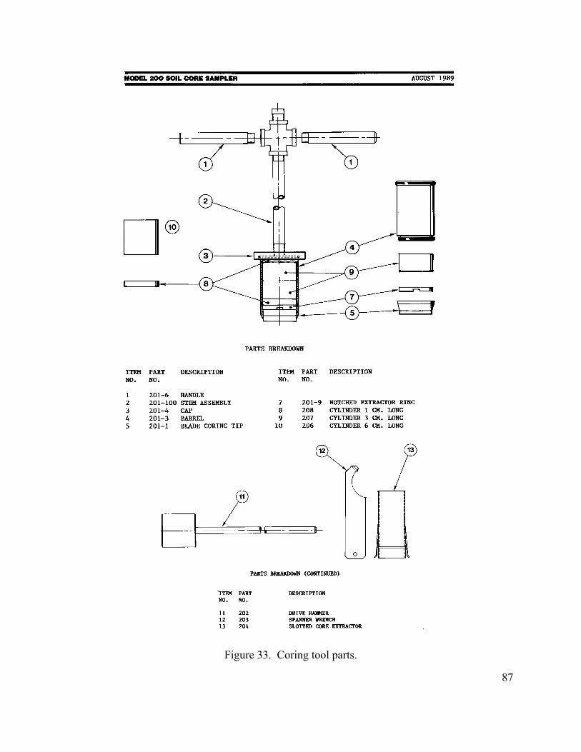
Figure 33. Coring tool parts.

87

11.7 Gravimetric Soil Moisture Sample Processing All GSM samples are processed to obtain a wet and dry weight. It is the sampling teams responsibility to deliver the can, fill out a sample set sheet, and record a wet weight at the field headquarters. A lab team will transport the samples to NSTL and place the samples in the drying ovens. They will perform the removal of samples from the oven, dry weighing, and can cleaning. All gravimetric soil moisture (GSM) samples taken on one day will be collected from the field headquarters in late afternoon or early the following morning. These samples will remain in the ovens until the morning of the second day (approximately 24 hours). Wet Weight Procedure

1. Turn on balance. 2. Tare. 3. Obtain wet weight to two decimal places and record on sheet. 4. Process your samples in sample numeric order. 5. Place the CLOSED cans back in the box. Arrange them sequentially. 6. Place box and sheet in assigned locations.

Dry Weight Procedure

1. Each day obtain a balance reference weight on the wet weight balance and the dry weight balance.

2. Pick up all samples from field headquarters. 3. Turn off oven and remove samples for a single data sheet and place on tray. 4. These samples will be hot. Wear the gloves provided 5. Turn on balance. 6. Tare. 7. Obtain dry weight to two decimal places and record on sheet. 8. Process your samples in sample numeric order. 9. All samples should remain in the oven for approximately 20-22 hours at 105oC. 10. Try to remove samples in the order they were put in. 11. Load new samples into oven. 12. Turn oven on. 13. Clean all cans that were removed from the ovens and place empty cans in boxes.

Check that can numbers are readable and replace any damaged or lost cans with spares.

14. Return the clean cans to the field HQ before 8:00 am the following day. Data Processing

1. Enter all data from the sheets into an Excel spreadsheet. One file per day, one worksheet per site.

88

2. There will be a summary file for each day that will contain the means and standard deviations.

3. All files are backed up with a floppy disk copy. 4. The summary file will be transmitted to a central collection point on a daily basis. 5. You may keep copies of raw data for any site that you actually sample at this

stage. You may not take any other data until quality control has been conducted

89

11.8 Watershed Site Soil Bulk Density and Surface Roughness All sites involved in gravimetric soil moisture sampling will be characterized for soil bulk density. The method used is a volume extraction technique that has been employed in most of the previous experiments and is especially appropriate for the surface layer. Four replications are made for each site. The Bulk Density Apparatus The Bulk Density Apparatus itself consists of a 12" diameter plexiglass piece with a 6" diameter hole in the center and three 3/4" holes around the perimeter. Foam is attached to the bottom of the plexiglass. The foam is three inches high and two inches thick. The foam is attached so that it follows the circle of the plexiglass. Figure 34 shows the basic components. Other Materials Required for Operation: Three 12" threaded dowel rods and nuts are used to secure the apparatus to the ground. A hammer or mallet is used to drive the securing rods into the ground. A bubble level is used to insure the surface of the apparatus is horizontal to the ground. A trowel is used to break up the soil and to remove the soil from the hole. Oven-safe bags are used to hold the soil as it is removed from the ground. The soil is left

in the bag when it is dried in the oven. Water is used to determine the volume of the hole. A plastic gas can is used to carry the water to the site. One gallon plastic storage bags are used as liners for the hole and to hold the water. A 1000 ml graduated cylinder is used to determine the volume of the water. Plastic is

best because glass can be easily broken in the field. A hook-gauge is used to insure water fills the apparatus to the same level each time.

Selecting and Preparing an Appropriate Site

1. Select a site. An ideal site to conduct a bulk density experiment is: relatively flat, does not include any rocks or roots in the actual area which will be tested and has soil which has not been disturbed.

2. Ready the site for the test. Remove all vegetation, rocks and other debris from the surface prior to beginning the test. Remove little or no soil when removing the debris.

90

Figure 34. How to take a bulk density sample. Bulk Density Procedure Securing the Apparatus to the Ground

1. Place the apparatus foam-side-down on the ground. 2. Place the three securing rods in the 3/4" holes of the apparatus. 3. Drive each dowel into the ground until they do not move easily vertically or

horizontally. (Figure 34a) Leveling the Apparatus Horizontally to the Ground

1. Tighten each of the bolts until the apparatus appears level and the foam is compressed to 1-1/2" to 2".

2. Place the bubble level on the surface of the apparatus and tighten or loosen the bolts in order to make the surface level. Place the level in at least three directions and on three different areas of the surface of the apparatus.

Determining the Volume from the Ground to the Hook Gauge

1. Pour exactly one liter of water into the graduated cylinder. 2. Pour some of the water into a plastic storage bag.

913. Hold the plastic bag so that the water goes to one of the lower corners of the bag.

4. Place the corner of the bag into the hole. Slowly lower the bag into the hole allowing the bag and the water to snugly fill all of the crevasses.

5. Slightly raise and lower the bag in order to eliminate as many air pockets as possible.

6. Lay the remainder of the bag around the hole. 7. Place the hook-gauge on the notches on the surface of the apparatus. 8. Add water to the bag until the surface of the water is just touching the bottom of

the hook on the hook-gauge. A turkey-baster works very well to add and subtract small volumes of water. Be sure not to leave any water remaining in the turkey-baster. (Figure 34b)

9. Place the graduated cylinder on a flat surface. Read the cylinder from eye-level. The proper volume is at the bottom of the meniscus. Read the volume of the water remaining in the graduated cylinder. Subtract the remaining volume from the original 1000 ml to find the volume from the ground surface to the hook-gauge.

10. Carefully transfer the water from the bag to the graduated cylinder. Hold the top of the bag shut, except for two inches at either end. Then use the open end as a spout. (It is best to reuse water, especially when doing multiple tests in the field.)

Loosening the Soil and Digging the Hole

1. Label the oven-safe bag with the date and test number and other pertinent information using a permanent marker.

2. Loosen the soil. The hole should be approximately six cm deep and should have vertical sides and a flat bottom. (The hole should be a cylinder: with surface area the size of the hole of the apparatus and height of six inches.)

3. Remove the soil from the ground and very carefully place it in the oven-safe bag. (Be careful to lose as little soil as possible.) (Figure 34c and d)

4. Continue to remove the soil until the hole fits the qualifications. Finding the Volume of the Hole

1. Determine the volume from the bottom of the hole to the hook-gauge as described in Determining the Volume from the Ground to the Hook-Gauge. Reusing the water from the prior measurement presents no potential problems and is necessary when performing numerous experiments in the field.

2. Subtract the volume of the first measurement from the second volume measurement. The answer is the volume of the hole.

Calculating the Density of the Soil

1. Dry the soil in an oven for at least 24 hours. 2. Determine the mass the soil. 3. Divide the mass of the soil by the volume of the hole. The answer is the density

of the soil.

92

Potential Problems and Solutions After I started digging I hit a rock. What should I do? The best solution is to start over in another location. Also, you can remove the rock from the soil and subtract the volume of the rock from the total volume of the water. You should never include a rock in the density of the soil. Rocks have significantly higher densities than soil and will invalidate the results. Roots, corn cobs, ants and even mole holes will also invalidate the results. If you find any of these things the best thing to do is start the test again at another site. After I began digging the hole I noticed one of the dowels wasn’t the apparatus firmly in place. Do I have to start over? Unfortunately, if you have already started digging you do have to start the experiment again. Replacing the dirt to find the volume between the ground surface and the hook-gauge will give an inaccurate volume and thus an inaccurate soil density. I noticed that the bag holding the water has a small leak. Is there anything I can do? If the leak began after you had already found the volume, it is not necessary to start again. The volume is being measured in the graduated cylinder. If you have already removed the appropriate volume of water leaks in the bag, it will not affect the results of the test. However, if you noticed the leak before finding the volume, you will have to start again. Surface Roughness • Take a photo along and across the rows at each BD location with the grid board. • The site and sample ID should be indicated in the photo.

93

11.9 Hydra Probe Soil Moisture and Apogee Temperature Sensor Installations Figure 35 shows a close up of the Hydra probe. As with the installation of any soil moisture measuring instrument, there are two prime considerations: the location the probe is to be installed at, and the installation technique. A copy of the instruction manual for the HP will be available at he field HQ and can also be found at http://hydrolab.arsusda.gov.

Figure 35. The Hydra probe used at the tower locations. Selecting a Location for the HP • The probe installation site should be chosen carefully so that the measured soil parameters

are "characteristic" of the site. • Make sure that the site will be out of foot traffic and is carefully marked and flagged. Installation of the HP • The installation technique aims to minimize disruption to the site as much as possible so that

the probe measurement reflects the “undisturbed site” as much as possible. o Dig an access hole. This should be as small as possible. o After digging the access hole, a section of the hole wall should be made relatively

flat. A spatula works well for this. o The probe should then be carefully inserted into the prepared hole section. The

probe should be placed into the soil without any side to side motion which will result in soil compression and air gaps between the tines and subsequent measurement inaccuracies. The probe should be inserted far enough that the plane formed where the tines join the probe head is flush with the soil surface.

94

o After placing the probe in the soil, the access hole should be refilled. o For a near soil surface installation, one should avoid routing the cable from the

probe head directly to the surface. A horizontal cable run of 20 cm between the probe head and the beginning of a vertical cable orientation in near soil surface installations is recommended.

• Other general comments are below. o Avoid putting undue mechanical stress on the probe. o Do not allow the tines to be bent as this will distort the probe data o Pulling on the cable to remove the probe from soil is not recommended. o Moderate scratches or nicks to the stainless steel tines or the PVC probe head

housing will not affect the probe's performance. Installation of the Apogee Surface Temperature Sensor A copy of the instruction manual for the Apogee sensor (Figure 36) will be available at he field HQ and can also be found at http://hydrolab.arsusda.gov. • Height • Target • Angle

Figure 36. Apogee thermal infrared sensor.

95

11.10 Vegetation Sampling Purpose of Sampling The purpose of vegetative sampling is to provide an estimate of the variation in the vegetative components in the corn and soybean fields across the SMEX02 study sites. Parameters

1. Plant height 2. Ground cover 3. Stand density 4. Phenology 5. Leaf area 6. Green and dry biomass

Sampling Locations Three sites within each field will be sampled during the course of the study to quantify the full range of vegetative cover. A minimum of three sampling times will be considered for SMEX02, a week before the study during the first week, and during the last week. Sites will be determined through aerial surveys of the sampling fields conducted during an early May and early June overflight. This is necessary since the spatial pattern across the field will depend upon the soil water distribution. For example, in the case of a wet spring the soils in the potholes of the landscape will be water stressed because of excess water and growth will be slowed, conversely in a dry year growth may be enhanced in the lower areas because of the increased soil water availability. Site Identification Sites will be identified with a unique site id made of the field number, within field site and row number, e.g., field number = V09 plus site 1 plus row 2 yields an id of V0912. The V will denote a vegetative sampling site to avoid any potential confusion with other measurement sites within the same field. Sampling Layout Each site will be identified with a flag in the right hand corner and a pole that extends above the crop height to aid in locating the site. Each sampling site will consist of a 10 row area by 10 m. This will provide adequate area for all sampling dates (see Figure 37). Sites will be located with GPS units and coordinates recorded for the corners of the site prior to the first sample collection. Sampling will not require the use of GPS but the right hand row of the sampling site will be flagged at the end row of the field so the sampling crews can travel down the rows.

96

Row direction

S SppaLth Tb P

X 10 9 X 8 7 X 6 5 X 4 3 X 2 1

3 m 3 m 3 m Flag First sample Second sample Third sample

X denotes sampling row

Figure 37. Vegetation sampling layout.

ampling Scheme

ampling sites are designed to provide a representative sample from the area of the field. One lant will be sampled from every other row for phenological stage and green and dry biomass (5 lants total). These same rows will be sampled for height, stand density, and row cover. Leaf rea will be measured at four locations (in-row, ¼ across row, ½ across row, ¾ across row) with I-2000. The first sampling position will be between the first row (flag location and the row to e left.

he first sampling time will begin on the end next to the flag, the second sampling time will egin 3 m down the row from the flag, and the third 6 m from the flag.

rotocols

1. Stand density Stand density will be determined by placing meter stick along the row in each of the 5 rows sampled. The meter stick will be placed at the center of a plant stem and that stem counted as the first plant. All plants within the one-meter length are to be counted. If a plant is at the end of the meter stick and more than half of the stalk extends beyond the end of the meter stick it is not counted. Counts are recorded onto the sampling sheet. 2. Phenology Phenological stage for corn and soybean will be determined using the standard phenological guide. The guide is attached as an appendix to this protocol. Plants from the sampling rows will be measured and recorded.

97

3. Height Height will be measured by placing a measuring rod on the soil surface in the row and recording the height of the foliage using a horizontal bar that just touches the upper leaves. One person will hold the measuring stick and the other determine the proper position of the horizontal bar.

4. Green and Dry Biomass To measure biomass a plant will be cut at the ground surface from each sampling row. The five plants for the sampling site will be placed into a plastic bag with a label for the sampling site. A separate tag with the sampling site id will be placed into the bag as additional insurance against damaged labels. These plants will be transported to the field facility for separation of the plant material into stalks and leaves for corn and stems and leaves for soybean. Corn plants can be separated into leaves and stalks in the field for easier transport to the laboratory. These plant parts will be placed into a bag for drying and marked with sample site id. Green biomass will be measured for both components (stalks or stems and leaves) by weighing the sample immediately after separation of the components. If the biomass has excess of moisture on the leaves and stalks this will be removed by blotting with a paper towel prior to weighing. Dry biomass will be determined after drying the plant components in ovens at 75C for 48 hours. 5. Leaf Area Leaf area will be measured with a LI-2000 (Figure 38) in the inter-row region at least one meter away from where the biomass sample was taken (5 sets of 4 across-row measurements). The LI-2000 will be set to average 4 locations into a single value so one observation is taken above the canopy and 4 beneath the canopy; in the row, ¼ of the way across the row, ½ of the way across the row and ¾ of the way across the row. This gives a good spatial average for row crops of partial cover. The observer always stands with their back to the sun if it is shining and a lens cap that blocks ¼ of the sensor view is always in place and positioned so the sun and the observer are never in the view of the sensor. The observer should always note if the sun was obscured during the measurement, whether the sky is overcast or partly cloudy with the sun behind the clouds. If no shadows could be seen during the measurement, then the measurement is marked “shaded”, if shadows could be seen during the measurement then the measurement is marked “sunny”. Conditions should not change from cloudy to sunny or sunny to cloudy in the middle of measurements. When measurements are made under sunny conditions, then someone will return to the site during a diffuse sky condition (near sunrise or sunset or when it is overcast within 2 days of the original measurement) and repeat the measurement to make sure that the presence of direct sun did not compromise the accuracy of the LAI measurement. Sunlit conditions can cause underestimates of LAI when LAI is low so factors must be obtained by which to adjust LAI measurements under sunny conditions. This does not necessarily mean all sites will have to be re-measured, but only sites representative of the sites measured.

98

Figure 38. The LAI-2000 instrument. 6. Photographs Photographs will be taken of plot area at the time of sampling. These will be collected with a digital camera. A marker board will be used to mark the plot, field location, and date. Photographs will be collected at an oblique angle (30-45º from horizontal) and at nadir at a height of a minimum of 1 m above the canopy. Cameras will be fixed to a telescoping pole to allow positioning above the canopy and a remote trigger to collect data. Three photos will be taken in each plot in this order; marker board, oblique, and nadir. 7. Ground reflectance Ground reflectance will be measured at each vegetative sampling site with a spectroradiometer. The spectroradiometer will be positioned above the plot area at a height to obtain a 50-100 cm2 viewing area. These data will be collected during the period from 10:00 – 1330 CST on clear days. These data will be recorded by plot with five readings per plot at different positions along row 10 of the plot. Data will be electronically recorded and stored and transferred into a ground reflectance database at the end of each day. Reflectance panel data are collected with a Spectrolon panel throughout the day to estimate reflectance values. Data would be collected with an Exotech radiometer mounted on a high-boy tractor in selected corn and soybean fields.

Data Recording

Data will be recorded onto the sampling sheet illustrated in Figure 39. Each field will have a separate notebook and data sheets for each sampling plot within the field. Each blank on the sheet will be filled in during the observation period. Data sheets will be maintained as part of the permanent experimental record to verify the data once it is entered into the computer.

99

Vegetative Sampling Date Observers

Time Row Spacing Row Direction Crop Photographs Taken

Sample

id

Stand density

Height

Phenology

Ground Cover

Green (g) Biomass

Dry (g) Biomass

Leaf Area Index

Sun/shade

(plants/m) (m) (%) Stem Leaf Stem Leaf V10102 x x x x V10104 x x x x V10106 x x x x V10108 x x x x V10110

Figure 39. Example of the vegetation sampling data sheet.

11.11 Plant Canopy Analyzer Measurements Setup • Connect sensor to X-connector (on left as viewed from keypad). Clean the lens carefully

with a lens brush. • Setup List:

o Verify X Cal data for X port. Serial No. should match sensor on X-connector. (FCT 01; 02)

o Set Resolution = HIGH. o Make sure time and date are correct (FCT 05)

• Operating Mode: o Set Op Mode= 1 sensor X (FCT 11) o Sequence= 1 above and 5 below (FCT 12) o Reps= 1 o Bad Reading= BEEP AND IGNORE (FCT 16)

• Verify that each ring (X1 thru X5) is responding to light. (BREAK) • View cap = 90 degrees. • Sky conditions:

o Diffuse illumination is ideal, but measurements can be made on sunny days with the following precautions:

o Make all Above and Below readings with your back to the sun and with the view cap blocking the sensor's view of you and the sun.

100

o Shade the sensor with your body to prevent reflections of the sun from influencing the readings.

o Shade the part of the canopy which is visible to the sensor with the umbrella. Sunlit leaves cause the sensor to underestimate LAI.

Sampling

1. Press LOG. Enter site number for SITE= prompt, e.g., LW01 or ER08. Enter plot+sample

for the SAMPLE= prompt, e.g., A10, A20, or C20. Add a zero to the sample number to indicate measurement is within the sampling frame.

2. Level the sensor above the canopy, shade the sensor from direct sun, and press the button on the sensor handle.

3. Note:Two beeps will be heard: one when the button is pressed and the other when the reading has been completed. Between the two beeps, keep the sensor level.

4. Put the sensor beneath the vegetation and level it. The sensor should view the same direction as the Above canopy reading. Press the button on the sensor handle.

5. Move the sensor about 15 cm diagonally (relative to the field of view of the sensor) and take another beneath the canopy reading. Repeat for 5 beneath the canopy readings. After the last reading the display will show COMPUTING....

6. Note: The first set of LAI measurements should be within the sampling frame. The subsequent measurements should be within 3 m of the frame.

7. Move to a new area outside the sampling frame and repeat steps #6-9 four times. SITE = stays the same (press enter to retain the value). SAMPLE= the last digit increments by one, e.g, A11, A12, A13, A21, A22, etc.

Downloading LAI-2000 files to a PC (see chapters 6 and 9 of Instruction Manual) 1. Use FCT 31 to set

• BAUD = 4800 • DATA BITS = 7 • PARITY = None • Xon/Xoff = No

2. Run communications program, PROCOMM, on personal computer. Configure the computer's RS-232 port to match the LAI-2000. Connect the computer and LAI-2000 with the appropriate cable. Specify the destination for the incoming data. c:\SMEX02\LAI\yymmddn.ext where yymmddn = year, month, day, name of team leader (c=Curry, r=Russ, w=Ward)..ext = format of output (.std = standard, .spr = spreadsheet format)

3. Output the LAI-2000 data files in the standard (.STD) and Spreadsheet (.SPR). formats. Backup files to a floppy disk.

4. Print the spreadsheet format files. 5. Clear the files after verifying that all files have been transferred.

101

11.12 Global Positioning System (GPS) Coordinates The acquisition of geographic coordinates at all sample point locations (e.g., WC and IA points, vegetation sites, and flux towers) is necessary for mapping of data in a Geographic Information System (GIS). A Garmin eTrex “sportsman” GPS will be used to collect location data. This unit has the capacity to store up to 500 geographic coordinates or waypoints and it is designed so that all key entries can be performed with the left hand alone. Accurate GPS data can be acquired 24 hours a day under all weather conditions. The only restraint is that the eTrex antenna--location determination is made at the site of the internal antenna--must have a clear view of the sky in all directions. Once accurate location data at a particular sample site has been acquired and confirmed, no additional measurements at that site will be needed. • All sampling points will be located using a handheld GPS.

o WC points o IA points o Vegetation samples o Flux towers

General Information Record eTrex ID number (etched on back cover), site and point ID, and latitude and longitude coordinates in field notebook.

Watershed and regional sites should be labeled as follows: Watershed: Site WC## and point ## (e.g., WC05-02) Regional: Site IA##

Carry at least two (2) extra AA alkaline batteries. The eTrex is configured to run in Battery Save mode which automatically turns the GPS receiver on and off to conserve power. In this mode, the eTrex should operate for approximately 22 hours. A “Battery Low” message will appear at the bottom of the screen when the unit has ten (10) minutes of battery life remaining. eTrex GPS Features (see Figure 40) UP/DOWN ARROW buttons: used to select options. ENTER button: used to confirm selections or data entry. PAGE button: switches between display screens (or “pages”) and functions as escape key. POWER button: turns eTrex GPS as well as display backlight on and off.

102

Data cable and Connector

AA Alkaline

Battery Cover

Power

PAGEUp Arrow Down Arrow Enter

Internal Antenna

Figure 40. GPS features. All eTrex operations are carried out from the four (4) “pages” (or display screens) Shown in Figure 41. The PAGE key is used to switch between pages. (The Map and Pointer Pages are used for navigation and will not be discussed further.)

Satellite Map Pointer Menu

Figure 41. GPS display screens or “pages”.

103

Setup at Headquarters Prior to Data Collection

1. Power unit on: Depress and hold power button until eTrex welcome screen appears and Satellite Page is displayed.

2. Confirm configuration parameters:

• PAGE to Menu screen; ARROW to Setup; press ENTER (Figure 42) • Use the following key sequence to check configuration parameters:

- ARROW to first parameter; press ENTER; - confirm values (see configuration values below); - press PAGE to return to Setup menu; - ARROW to next parameter, etc.

• The following are the parameters and required settings; - Time = Format: 24 Hour; Zone: US-Central; (UTC Offset: -6:00);

Daylight Saving: Auto - Display = Timeout: 15 sec. - Units = Position Format: hddd.dddddo; Map Datum: WGS 84; Units:

Metric; North Reference: True - Interface = I/O Format: Garmin - System = Mode: Battery Save

Figure 42. GPS Menu page.

3. Turn eTrex off after GPS data collection by depressing and holding POWER button until

screen blanks. Important Note: Geodetic datums mathematically describe the size and shape of the earth and provide the origin and orientation of coordinate systems used in mapping. Hundreds of datums are currently in use and particular attention must be paid to what datum is used during GPS data collection. The Global Positioning System is based on the World Geodetic System of 1984 (WGS84). However, popular map products such as USGS 1:24,000 topo sheets originally used the North American Datum of 1927 (NAD27). Most of the maps in this series have been updated to the North American Datum of 1983 (NAD83). Fortunately, there is virtually no practical difference between WGS84 and NAD83. Yet significant differences exists between

104

NAD27 and NAD83. (In Iowa, a north-south displacement of approximately 215m occurs between NAD27 and NAD83.) All geographic coordinates collected with the eTrex GPS should be acquired using the following parameters: latitude/longitude (decimal degrees), WGS84 datum, meters, true north. Various coordinate conversion software packages such as the Geographic Calculator ($500) or NOAA’s Corpscon (free) exist which allow the conversion of geodetic (latitude and longitude) coordinates into planar (UTM or State Plane) coordinates for GIS mapping. GPS Field Data Collection

1. Power unit on: Depress and hold power button until eTrex welcome screen appears and Satellite Page is displayed (Figure 43). Wait until text box at top of screen reads “READY TO NAVIGATE” before continuing.

Wait until “READY TO NAVIGATE is displayed AND Accuracy is <= 10 m

(Up to 5 minutes at a new location; 15-45 seconds on subsequent visits.)

Figure 43. GPS Satellite Page.

2. Adjust screen backlight and contrast, if necessary.

• Turn backlighting on by quickly pressing and releasing POWER button from any screen. (To save power, the backlight remains on for only 30 seconds.); AND/OR,

• Adjust screen contrast by pressing UP (darker) and DOWN (lighter) buttons from Satellite Page.

3. Initiate GPS point data collection:

• PAGE to Menu screen (Figure 42); Arrow to Mark; press ENTER. (Shortcut: press and hold ENTER button from any screen to get to Mark Waypoint page below.)

• ARROW to alphanumeric ID field (Figure 44); press ENTER. Use ENTER and UP/DOWN buttons to edit ID, if necessary. (Waypoint ID increments by one (1) automatically.)

• Record latitude (North) and longitude (West) coordinates displayed at bottom of screen into field notebook. Do not rely on electronic data download to save data points!

• ARROW to OK prompt; press ENTER to save point coordinates electronically.

105

Copy geographic coordinates into field notebook

ARROW to OK prompt; press ENTER to store coordinates.

ID field; edit ID using ENTER and UP/DOWN buttons

Figure 44. GPS Mark Waypoint Page.

4. Turn eTrex off after GPS data collection by depressing and holding POWER button until screen blanks.

Electronic Data Downloading Electronic data downloading will be performed at field headquarters by assigned person. Connect PC data cable by sliding keyed connector into shoe at top rear of eTrex (under flap); power eTrex on. Launch Waypoint.exe GPS => Port => Com? Waypoints => Download File => Save => Waypoint Select Save as type: Comma Delimited Text File

106

12 References Ahmed, N. U., 1995. Estimating soil moisture from 6.6 GHz dual polarization, and/or satellite derived vegetation index. Int. J. of Remote Sensing, 16: 687-708.

Albertson, J. D. and M. B. Parlange, 1999. Natural integration of scalar fluxes from complex terrain, Adv. in Water Resour., 23:239-252.

Albertson, J. D., W. P. Kustas and T.M. Scanlon, 2001. Large eddy simulation over heterogeneous terrain with remote sensed land surface conditions. Water Resour. Res., 37:1939-1953.

Anderson, M. C., J. M. Norman, G. R. Diak and W. P. Kustas, 1997. A two-source time Integrated model for estimating surface fluxes for thermal infrared satellite observations. Rem. Sens. Environ., 60:195-216. Anderson, M., J. M. Norman T. P. Meyers and G. R. Diak, 2000. An analytical model for estimating canopy transpiration and carbon assimilation fluxes based on canopy light-use efficiency. Agric. For. Meteorol., 100:265-289. Armatys, M., D. Masters, A. Komjathy, P. Axelrad, and J. Garrison, 2000. Exploiting GPS as a new oceanographic remote sensing tool, Proc. Institute of Navigation Technical Meeting, Anaheim, CA, 26-28 January, 2000. Avissar, R. and T. Schmidt, 1998. An evaluation of the scale at which ground-surface heat flux patchiness affects the convective boundary layer using Large-Eddy Simulation, J. Atmos. Sci., 55:2666-2689.

Avissar, R., E. W. Eloranta, K. Gürer and G. J. Tripoli, 1998. An evaluation of the Large-Eddy Simulation option of the Regional Atmospheric Modeling System in simulating a convective boundary layer: A FIFE case study, J. Atmos. Sci., 55:1109-1130.

Bayler G.M., R.M. Aune and W. L. Raymond, 2000. NWP cloud initialization using GOES sounder data and improved modeling of nonprecipitating clouds. Mon. Wea. Rev., 128:3911-3920. Burns, B. A., X. Wu and G. R. Diak, 1997. Effects of precipitation and cloud ice on brightness temperatures in AMSU moisture channels. Int. J. Rem. Sens., 35:1429-1437. Cai, X. -M., 1999. Large-Eddy Simulation of the convective boundary layer over an idealized patchy urban surface, Q.J.R. Meteorol. Soc., 125:1427-1444. Diak, G. R., 1990. Evaluation of heat flux, moisture flux and aerodynamic roughness at the land surface from knowledge of the PBL height and satellite-derived skin temperatures. Agr. For. Meteor., 52:181-198.

107

Diak, G. R., D. Kim, M. S. Whipple and X. Wu, 1992. Preparing for the AMSU. Bull. Amer. Meteor. Soc., 73:1971-1984.

Diak, G. R., C. J. Scheuer, M. S. Whipple and W. L. Smith, 1994. Remote sensing of land-surface energy balance using data from the High-Resolution Interferometer Sounder (HIS): A simulation study, Rem. Sens. Environ., 48:106-118.

Diak, G. R., R. M. Rabin, C. M. Neale and K. P. Gallo, 1995. Regional-scale comparisons of vegetation and soil wetness with surface energy budget properties from satellite and in-situ observations. Remote Sensing Reviews, 12:355-382.

Diak, G. R., W. L. Bland and J. R. Mecikalski, 1996. A note on first estimates of surface insolation from GOES-8 visible satellite data. Agr. For. Meteor., 82:219-226.

Diak, G. R., M. C. Anderson, W. L. Bland, J. M. Norman, J. R. Mecikalski and R. M. Aune, 1998. Agricultural management decision aids driven by real-time satellite data. Bull. Amer. Meteor. Soc. 79:1345-1355.

Diak, G. R., W. L. Bland, J. R. Mecikalski, and M. C. Anderson, 2000. Satellite estimates of longwave radiation for agricultural applications. Agric. For. Meteorol., 103:349-355.

Early, D. S., and D. G. Long, 2001. Image reconstruction and enhanced resolution imaging from irregular samples, IEEE Transactions on Geoscience and Remote Sensing, 39:291-302. Eastman, J. L., R. A. Pielke and D. J. McDonald, 1998. Calibration of soil moisture for large-eddy simulations over the FIFE area, J. Atmos. Sci., 55:1131-1140.

Eichinger, W. E., D. I. Cooper, L. C. Chen, L. Hipps and C.-Y. J. Kao, 2000. Estimation of spatially distributed latent heat flux over complex terrain from a Raman lidar. Agri. For. Meteorol., 105:145-159.

Flēchard, C. R., R. L. Desjardins, J. I. MacPherson, T. Zhu, D. Wang and E. Pattey, 2001. Measuring trace gas fluxes on a regional scale using airborne relaxed eddy accumulation, Proceedings of the 11th AMS.Symposium on Meteorological Observations and Instrumentation, Albuquerque, January 14-18, 2001.

Giorgi, F., and R. Avissar, 1997. Representation of heterogeneity effects in earth system modeling: experience from land surface modeling. Rev. Geophys., 35,:413-437.

Hadfield, M. G., W. R. Cotton and R. A. Pielke, 1991. Large-eddy simulations of thermally forced circulations in the convective boundary layer. Part I: A small-scale circulation with zero wind, Bound.- Layer Meteorol., 57: 79-114.

Hadfield, M. G., W. R. Cotton and R. A. Pielke, 1992. Large-eddy simulations of thermally forced circulations in the convetive boundary layer. Part II: The effect of changes in wavelength and wind speed, Bound.- Layer Meteorol., 58,:307-27.

108

Hall, F. G., K. F. Huemmrich, S. J. Geotz, P. J. Sellers, J. E. Nickerson, 1992 Satellite remote sensing of surface energy balance: success, failures and unresolved issues in FIFE, J. Geophys. Res. 97(D17):19,061-19,090.

Hechtel, L. M., C. -H. Moeng and R. B. Stull, 1990. The effects of nonhomogeneous surface fluxes on the convective boundary layer: A case study using large-eddy simulation, J. Atmos. Sci., 47:1722-1741.

Hu, Z., S. Islam, and L. Jiang, 1999. Approaches for aggregating heterogeneous surface parameters and fluxes for mesoscale and climate models. Bound.-Layer Meteorol., 93:313-336.

Jackson, T. J., 1997. Soil moisture estimation using SSM/I satellite data over a grassland region. Water Resources Research, 33: 1475-1484.

Jackson, T. J. and A. Y. Hsu, 2001. Soil moisture and TRMM microwave imager relationships in the Southern Great Plains 1999 (SGP99) experiment, IEEE Trans. on Geoscience and Remote Sensing, 39:1632-1642. Jackson, T. J., T. J. Schmugge, and P. E. O'Neill. 1984. Passive microwave remote sensing of soil moisture from an aircraft platform. Remote Sensing of Environment, 14:135-152.

Jackson, T. J., D. M. Le Vine, C. T. Swift, T. J. Schmugge, and F. T. Schiebe, 1995. Large area mapping of soil moisture using the ESTAR passive microwave radiometer in Washita'92. Remote Sensing of Environment, 53: 27-37.

Jackson, T. J., D. M. Le Vine, A. Y. Hsu, A. Oldak, P. J. Starks, C. T. Swift, J. D. Isham, and M. Haken, 1999. Soil moisture mapping at regional scales using microwave radiometry: The Southern Great Plains hydrology experiment. IEEE Trans. Geosci. Remote Sens., 37, 2136-2151

Jackson, T. J., A. J. Gasiewski, A. Oldak, M. Klein, E. G. Njoku, A. Yevgrafov, S. Christiani, and R. Bindlish, 2002. Soil Moisture Retrieval Using the C-Band Polarimetric Scanning Radiometer During the Southern Great Plains 1999 Experiment, submitted to IEEE Trans. on Geoscience and Remote Sensing. Kustas, W. P., X. Zhan and T. J. Schmugge, 1998. Combining optical and microwave remote sensing for mapping energy fluxes in a semiarid watershed. Rem. Sens. of Env., 64:116-131.

Kustas, W. P., X. Zhan and T. J. Jackson, 1999a. Mapping surface energy flux partitioning at large scales with optical and microwave remote sensing data from Washita ‘92, Water Resour. Res., 35:265-277.

Kustas, W. P., J. H. Prueger, K. S. Humes and P. J. Starks, 1999b. Estimation of surface heat fluxes at field scale using surface layer versus mixed layer atmospheric variables with radiometric temperature observations. J. of App. Meteorol., 38: 224-238.

Kustas, W. P., G. R. Diak and J. M. Norman, 2000. Time difference methods for monitoring regional scale heat fluxes with remote sensing. In Lakshmi, V., J. Albertson, and J. Schaake

109

(ed), Observations and Modeling of Land Surface Hydrological Processes. Water Science and Applications Series, 3: 15-29, American Geophysical Union.

Leese, J., T. Jackson, A.Pitman, and P. Dirmeyer, 2001. GEWEX/BAHC international workshop on soil moisture monitoring, analysis and prediction for hydrometeorological and hydroclimatological applications. Bulletin of the American Meteorological Society, 82:1423-1430. 2001. Le Vine, D.M., T. T. Wilheit, R. E. Murphy, and C. T. Swift, 1989. A multifrequency microwave radiometer of the future. IEEE Trans. Geosci. Remote Sens., 27:193-199. Le Vine, D. M., M. Kao, A. B. Tanner, C. T. Swift, and A. Griffis, 1990. Initial results in the development of a synthetic aperture microwave radiometer. IEEE Trans. Geosci. Remote Sens., 28:614-619. Le Vine, D. M., A. J. Griffis, C. T. Swift, and T. J. Jackson, 1994. ESTAR: A synthetic aperture microwave radiometer for remote sensing applications. IEEE Proc., 82:1787-1801. Le Vine, D. M., T. J. Jackson, C. T. Swift, M. Haken, and S. W. Bidwell, 1994. ESTAR measurements in the Southern Great Plains experiment (SGP99). IEEE Trans. Geosci. Remote Sens., 39:1680-1685. MacPherson, J. I., Marcotte, D. L, and J. E. Jordan, 2001. The NRC atmospheric research aircraft. Canadian Aeronautics and Space Journal, 47:147-157. Mahfouf, J.-F., 1991. Analysis of soil moisture from near-surface parameters: a feasibility study. J. Appl. Meteorol., 30:1534-1547.

Masters, D., P. Axelrad, V. Zavorotny, S. J. Katzberg, and W. Emery, 2000. GPS signal scattering from land for moisture content determination, Proc. IEEE IGARSS 2000, Honolulu, HI, July 24-28, 2000. Masters, D., P. Axelrad, V. Zavorotny, S. J. Katzberg, and F. Lalezari, 2001. A passive GPS bistatic radar altimeter for aircraft navigation, Proc. ION GPS 2001, Salt Lake City, 2001. Mecikalski, J. R., G. R. Diak, J. M. Norman and M. C. Anderson, 1997. Evaluation of Regional-scale land surface sensible heating using shelter-level measurements of atmospheric temperature combined with analyses of upper-air data. Agr. For Meteor., 88:100-110. Mecikalski, J. R., G. R. Diak, M. C. Anderson and J. M. Norman, 1999. Estimating fluxes on continental scales using remotely-sensed data in an atmospheric-land exchange model. J. Appl. Meteorol., 38:1352-1369.

Monteith, J. L., 1977. Climate and the efficiency of crop production in Britain. Philos. Trans. R. Soc. London B., 281: 277-294.

110

Neale, C. M. U. and B. G. Crowther, 1994. An airborne multispectral video/radiometer remote sensing system: development and calibration. Rem. Sens. Environ., 48:1-25.

Njoku, E. G. and L. Li, 1999. Retrieval of land surface parameters using passive microwave measurements at 6 to 18 GHz. IEEE Trans. Geosc. Rem. Sens., 37:79-93.

Norman, J.M. and T.J. Arkebauer, 1991. Predicting Canopy Light-Use Efficiency from Leaf Characteristics. pp. 75-94, in K. Boote and R. Loomis (Ed.) Modeling Crop Photosynthesis: From Biochemistry to Canopy. ASA Spec Pub., Madison WI.

Norman, J. M., L. C. Daniel, G. R. Diak, T. E. Twine, W. P. Kustas, A. N. French and T. J. Schmugge, 2000b. Satellite estimates of evapotranspiration on the 100-m pixel scale. IEEE IGARRS 2000 Proceedings., Vol. IV, 1483-1485.

Norman, J. M., W. P. Kustas and K. S. Humes, 1995. A two-source approach for estimating soil and vegetation energy fluxes from observations of directional radiometric surface temperature, Agric. and Forest Meteorol., 77:263-293.

Norman, J. M., W. P. Kustas, J. H. Prueger and G.R. Diak, 2000a. Surface Flux Estimation Using Radiometric Temperature: A double-difference method to minimize measurement errors. Water Resour. Res., 38:2263-2274.

Piepmeier, J. R. and A. J. Gasiewski, 2001. High-resolution passive microwave polarimetric mapping of ocean surface wind vector fields, IEEE Trans. Geosci. Remote Sensing, 39:606-622. Raymond, W. H., 1988. High-order low-pass implicit tangent filters for use in finite area calculations. Mon. Wea. Rev., 116:2132-2141.

Raymond, W. H., 1993. Moist wind relationships. Mon. Wea. Rev., 121:1992-2003.

Raymond, W. H., 1994. Diffusion and numerical filters. Mon. Wea. Rev., 22:757-761.

Schmugge, T. J., W. P Kustas and K. S. Humes, 1998. Monitoring land surface fluxes using ASTER observations, IEEE Trans. Geo. Remote Sens. 36:1-10.

Sellers, P. J., D. A. Randall, G. J. Cozzatz, J. A. Berry, C. B. Field, D. A. Dazlich, C. Chang, G. D. Collelo and L. Bounoua, 1996. A revised land surface parameterization (SiB2) for atmospheric GCMs. Part I: Model Formulation. J. Climate, 9:676-705.

Spencer, M. W., C. Wu, and D. G. Long, 2000. Improved Resolution Backscatter Measurements with the SeaWinds Pencil-Beam Scatterometer, IEEE Transactions on Geoscience and Remote Sensing, 38:89-104. Teng, W. L., J. R. Wang, and P. C. Doriaswamy, 1993. Relationship between satellite microwave radiometric data, antecedent precipitation index, and regional soil moisture. Int. J. of Remote Sensing, 14: 2483-2500.

111

Thompson, A. R., J. M. Moran, and G. W. Swenson, 1986. Interferometry and synthesis in radio astronomy, New York; Wiley.

Vining, R.C., and B. L. Blad, 1992. Estimation of sensible heat flux from remotely sensed canopy temperatures, J. Geophys. Res., 97:18,951-18,954.

Wang, J. R., 1985: Effect of vegetation on soil moisture sensing observed from orbiting microwave radiometers. Remote Sens. Environ., 17:141-151. Wang, J. R., P. E. O'Neill, T. J. Jackson, and E. T. Engman, 1983. Multifrequency measurement of thermal microwave emission from soils: the effects of soil texture and surface roughness, IEEE Trans. on Geoscience and Remote Sensing, 21:44-55. Wen, J. and Z. Su, 2001. The variation of soil moisture estimated from ESA windscatterometer data, in Z. Su and R. Roerink (eds.) Active microwave remote sensing of soil moisture for initialization of numerical weather prediction, Publications of the National Remote Sensing Board (BCRS), USP-2, 01-04. Wilson, W. J., S. H. Yueh, S. J. Dinardo, S. L Chazanoff, A. Kitiyakara, F. K. Li, and Y. Rahmat-Samii, 2001. Passive active L- and S-band (PALS) microwave sensor for ocean salinity and soil moisture measurements. IEEE Trans. on Geoscience and Remote Sensing, 39:1039 –1048.

Wu, X. and W. L. Smith, 1992. Assimilation of ERBE data with a nonlinear programming technique to improve cloud-cover diagnosis. Mon. Wea. Rev., 9:2009-2024.

Wu, X., G. R. Diak, C. M. Hayden and J. A. Young, 1994. Short-range precipitation forecasts using assimilation of simulated satellite water vapor profiles and cloud liquid water. Mon. Wea. Rev., 123:347-365.

Yang, R., M. J. Fennessy and J. Shukla, 1994. The influence of initial soil wetness on medium-range surface weather forecasts. Mon. Wea. Rev., 122:L471-485.

Zavorotny, A. Voronovich, 2000. Scattering of GPS signals from the ocean with wind remote sensing application, IEEE Trans Geosci. Remote Sens.,.38:951-964.

112

13 INVESTIGATOR ABSTRACTS

113

Flux Measurement and Large Eddy Simulation of Land-Atmosphere Exchange John D. Albertson and William P. Kustas John D. Albertson, Civil and Environmental Engineering, Duke University, Box 90287, Hudson Hall, Durham, NC 27708-0287, john.albertson@duke.edu We will field several eddy covariance towers to measure water, energy, and carbon fluxes in representative fields within the footprint of the aircraft operating over the Walnut Creek Watershed in Ames, Iowa. Our measurements will be conducted in coordination with the other surface flux efforts, as overseen by John Prueger. Furthermore, through our participation in the Kustas et al. NASA project our measurements will be coordinated with the aircraft flux, aircraft remote sensing, and Lidar operations. Also, under the Kustas et al. NASA project we will be conducting Large Eddy Simulation (LES) of the Atmospheric Boundary Layer (ABL) dynamics over the remotely sensed land surface fields. Our tower measurements will include: upward and downward directed short-wave, long-wave, and photosynthetically-active radiation; sensible heat, latent heat, and CO2 fluxes; radiometric surface temperature; air temperature and humidity; wind speed, direction, and friction velocity (u*); precipitation; soil moisture; soil temperature; soil heat flux. The LES work will be based on our LES-Remote Sensing approach (Albertson et al., WRR, 37, 1939-1953, 2001). We will simulate land surface flux fields over the region and ABL development and structure. Detailed atmospheric structure simulated by the LES will be evaluated in the context of the Lidar observations. Joint analysis of the LES results and Lidar data will be conducted to explore mixing of the ABL over heterogeneous terrain, assess feedback effects of the heterogeneity on land-atmosphere coupling, and test spatial scaling hypotheses over complex terrain. Remotely sensed fields of surface cover, temperature, and moisture, and balloon and lidar profiles of the ABL are critical data needs to support the LES work.

114

115

Operational Use of Scatterometer Data over Land to Improve Hydro-Meteorological Forecasts Mark A. Bourassa1, James J. O’Brien1, David E. Weissman2, Jeffrey Tongue3, Tom Adams4 1. Center for Ocean-Atmospheric Studies, Florida State University, Tallahassee FL 32306-2840, bourassa@coaps.fsu.edu, (850) 644-6923,FAX: (850) 644-4841 obrien@coaps.fsu.edu, (850) 644-4581 2. Hofstra University, eggdew@hofstra.edu, (516) 463-5546, FAX: 631-269-5920 3. National Weather Service WFO, 175 Brookhaven Ave., Upton, NY 11973, Jeffrey.Tongue@noaa.gov, (516) 924-0593 x 224, FAX: (516) 924-0593 x 224 4. Ohio River Forecast Center, National Weather Service, 1901 S. State Route 134, Wilmington, OH 45177, (937) 383-0527, FAX: (937) 383-0038

This project will create a new capability for remote sensing of surface moisture, and study the use of these observations in weather forecasting, hydrology, and forestry. The combinations of satellite-derived surface moisture measurements, which have good temporal coverage (the wide 1800 km swath width and orbit selection results is approximately twice daily sampling) and high spatial resolution, with other National Weather Service resources are expected to lead to major enhancements land weather forecasts. Results of this research will enable conventional rain data (e.g., NEXRAD precipitation) to be used to improve the knowledge (and hence models) of retention and runoff in surface hydrology. The SMEX02 data desired for our study are ground water content observations, which can them be used for validation/calibration of our algorithms. The National Aeronautics and Space Administration recently launched a new, polar orbiting satellite radar, named “SeaWinds” on the QuikSCAT spacecraft. This instrument is a specialized microwave radar designed to measures near surface wind speed and direction under all weather and cloud conditions over the earth’s oceans; however, it also operates over land. The swath width of the radar is 1800 km. Wind vector estimates are averaged over each 25x25km square area within the swath; however, high-resolution techniques have been used to obtain 10x10km backscatter products from a single pass over land (Spencer et al. 2000; Early and Long 2001). Surface locations are illuminated an average of 2 times each day with one satellite. Another SeaWinds instrument is scheduled to be launched in November 2002, and it is anticipated that the orbits will be designed to provide ~4 times daily sampling in ~6 hour intervals. These examples of sampling are appropriate for the latitudes of the United States of America; sampling will be a little worse in the tropics, and much better near the poles. Through a cooperative effort between NASA/JPL and NOAA/NESDIS Office of Research and Applications near real-time data is available for rapid transfer to selected NWS operational offices. We have identified an unanticipated application of scatterometer observations: there is a signal related to the moisture in the upper several centimeters of the ground. A principal objective of our project is to facilitate the implementation and evaluation of these observations, at the level of the individual Weather Forecast Offices, state climatologists (the PI, O’Brien, is the Florida State climatologist), and numerical weather prediction (NWP). This project will implement mutual education and training between NWS Scientific & Operations Officers, hydrologists, and Scatterometer researchers in ways that had not been envisioned when the satellite was designed.

116

Preliminary results (see figure below) indicate that there is a substantial signal in the backscatter (the signal returned to the satellite) related to moisture in the surface or in vegetation. The integrated depth of surface moisture to which the satellite instrument responds will be approximately 1cm: it will measure the moisture content very close to the surface. Such observations should be ideal for NWP initialization, for which knowledge of surface moisture content is poorly known, and for which improvements in accuracy have been anticipated to lead to substantial improvements in NWP accuracy. We anticipate that the value of such observations will increase with time, as the resolution of NWP models increases, and local changes in surface moisture content are expected to have greater impacts. We will explore a theoretically-based model, and calibrate this model with in situ ground observations products through several projects. The resulting estimates of moisture content will be used studies involving NWP, hydrology, moisture climatology (drought impacts), forestry (fire risk), and estimates of mosquito-related problems. The theoretical developments will be lead by David Wiessman, NWP and hydrology applications will be pursued by the NWS, and the applications to drought, forestry, and mosquitoes will be undertaken a COAPS and related to our routine activities in these areas.

Stronger backscatter from wet ground.

-2.5 -2.0 –1.5 –1. -0.5 –.25 2.5 0.5 1.0 1.5 2.0

TS Alison

NEXRAD radar image of TS Alison and associated rain.

Change in H-pol σo (dBZ)(Wet period – dry period)

Stronger backscatter from wet ground.

-2.5 -2.0 –1.5 –1. -0.5 –.25 2.5 0.5 1.0 1.5 2.0

TS Alison

NEXRAD radar image of TS Alison and associated rain.

Change in H-pol σo (dBZ)(Wet period – dry period)

Figure - Change in QSCAT H-pol so (after a dry period; wet case minus dry case) due to TS Alison. Backscatter is binned in 0.25 degree bins, from 3 hour periods on separate days.

117

Scaling Characteristics of Remotely Sensed Vegetation, Surface Radiometric Temperature, and Derived Surface Energy Fluxes N. A. Brunsell and R. R. Gillies Nate Brunsell, Dept. of Plants, Soils, and Biometeorology, Agricultural Science 322, Utah State University 4820 University Blvd., Logan, UT 84322-4820 The proposed research entails examining the spatial variability observed over multiple scales of remotely sensed data. These will include airborne, Landsat TM, and AVHRR. Wavelet multiresolution analysis will be used to examine the characteristics of vegetation and surface temperature over the range of scales. A Soil-Vegetation-Atmosphere-Transfer (SVAT) model will be used to derive surface energy fluxes using the "Triangle" method and the scaling characteristics of the resultant fluxes will also be examined. In addition, the co-spectra will be used to examine the correlation between remotely sensed input and the derived surface fluxes. The proposed research will aid in the assimilation of coarse resolution (e.g., AVHRR) remotely sensed data into regional meteorological models.

118

119

Optimizing Land-Atmosphere Interaction Models For Use With Data Assimilation Anthony Cahill Department of Civil Engineering, Texas A&M University, 3136 TAMU, College Station, TX 77843-3136, Phone: 979-862-3858, Fax: 979-862-1542 This project seeks to explore what approach to modeling the land-atmosphere interaction is best for use with data assimilation. There are a number of different models for estimating the energy fluxes and the moisture and temperature states at the land surface. These models are of varying complexity, and simulation the transport processes in different ways. Which land-atmosphere interaction models give the best results with different methods of data assimilation is an open question. In fact, how to define "best" is itself an open question. In this work, the PI will develop a method a estimating the merit of a data assimilation-land surface model set, and using the data collected in the SMEX 02 experiment, will determine which approaches are best. The PI will be part of the flux tower data collection team at SMEX 02, and this data will be used in the analysis proposed here. Other data to be used will include the aircraft flux and soil brightness temperature measurements. It is assumed that a means of determining the "best" set of methods can be done by minimizing a discrepancy measure, such as is done with AIC. Other factors that must be kept in mind in the analysis include the different scales on which the measurements are taken, and the difficulty of estimating measurement error for remotely sensed measurements. The overall contribution of this project will be guidance for future work in the application data assimilation of satellite measurements in land surface hydrology, when the satellite measurements become available.

120

121

Assessing the Role of Distributed Hydrologic Modeling for Validation of AMSR-E Soil Moisture Products Wade Crow USDA-ARS Hydrology and Remote Sensing Laboratory, 104 Bldg. 007, BARC-West, Beltsville, MD, 20705. The coarse spatial resolution of spaceborne microwave radiometers (> 30 km) poses a severe challenge for efforts to validate soil moisture products derived from such observations. Validation based on point-scale observations require upscaling strategies (e.g. kriging, interpolation, weighted averaging) capable of converting local observations into meaningful predictions of soil moisture at the footprint-scale. The success of any given strategy hinges largely on obtaining an accurate of the underlying autocorrelation within the soil moisture field and the manner in which soil moisture variability is cross-correlated with observable land surface attributes (i.e. topography, soil and vegetation cover). Given the practical difficulties in obtaining in situ soil moisture data of sufficient length and extent to provide such descriptions, recent interest has focused on the use of distributed hydrologic models to bridge the scale gap between in situ observations and footprint-scale retrievals. The assumption underlying such approaches is that hydrologic models are capable of realistically capturing landscape-scale soil moisture heterogeneity. Regional soil moisture observations during SMEX02 provide an excellent opportunity to test such an assumption and clarify the potential role of distribution hydrologic modeling for validation of spaceborne retrievals and/or the design of optimal in situ observation networks. Specific goals include: 1) Intercomparison of statistical and explicit representations of surface soil moisture heterogeneity obtained from field observations, retrievals, and hydrologic models during SMEX02. 2) Development and testing of model-based strategies for accurately upscaling a subset of regional soil moisture observations up to the AMSR-E footprint scale.

122

123

Energy Balance and Crop Yield Studies at Walnut Creek Watershed Paul Doraiswamy, William Kustas Hydrology and Remote Sensing Laboratory, USDA- ARS, Beltsville Maryland Jerry Hatfield and John Prueger National Soil Tilth Laboratory, USDA-ARS, Ames, Iowa Objective 1: Daily Energy Balance and Evapotranspiration mapping for the Watershed using a dynamic energy balance model Model required Inputs: Hourly/Daily climate data, vegetation classification, LAI, Canopy reflectance (ground and airborne), surface temperature (ground and airborne) and TM Landsat imagery. Outputs: Parameter maps for the Watershed of ET, Energy Balance and Crop Water Stress. Objective 2: Corn and Soybean Crop Yields using parameters retrieved from remote sensing with crop simulation models. Inputs: Daily climatic data, vegetation classification , LAI, soil classification Baseline nitrogen levels, Management practices and crop yields at fields selected for monitoring vegetation parameters. Outputs: Crop yields at watershed and county levels Objective 3: Scaling up ET and Crop Yields from field to watershed. Data acquired for Objectives 1 and 2 will be used in models to scale up to the watershed level. Inputs: Daily climatic data, crop phenology, vegetation classification, leaf area index, soil classification, baseline nitrogen levels. Satellite and available aircraft imagery for visible, near IR and thermal. Outputs: ET and crop yield maps for the watershed. Planned Ground Measurements at Walnut Creek • Vegetation classification • Corn and soybean canopy architecture parameters (one time in July) • Canopy reflectance (one time in July) Planned satellite data acquisition and processing • ETM Landsat- 30 m visble/near IR sharpened to 15 m - 90 m surface temperature • MODIS- 250 m visible and near IR - 1 km surface temperature • AVHRR- 1 km (surface temperature and visible/near IR)

124

Measurements Required from Other Investigators Crop measurements LAI, biomass, crop phenological, crop yields Soil measurements Soil physical properties at field or water shed levels Soil chemical (C,N) properties at field or water shed scales Soil moisture Surface Measurements Water and CO2 fluxes from tower measurements Climate measurements from towers Aircraft Measurements Visible near IR reflectances Surface temperature Soil moisture

125

126

127

Field Observations of Soil Moisture Variability from the Point to Remote Sensing Footprint Scale Jay Famiglietti, UC Irvine, jfamigli@uci.edu, tel: 949-824-9434; fax: 949-824-3874 Graduate student participants: Aaron Berg, UC Irvine, berga@uci.edu Sally Holl, UC Irvine, sholl@uci.edu Dongryeol Ryu, UC Irvine, dryu@uci.edu Ki-Weon Seo, UT Austin, kiweon@speer.geo.utexas.edu Our field studies will build on our previous work during SGP97 and SGP99. In 1997 we made detailed observations of surface soil moisture variations within a dozen ground truth (quarter section) sites, and carefully analyzed the data in 6 of these fields. We found that soil moisture variability increased with increased drying and that the distributions followed predictable forms. In 1999 we studied soil moisture variability across scales, from 2.5 x 2.5 m plots to a 1.6 x 1.6 km (full section) area, quadrupling the size of the areas studied in 1997. Results indicated that variability increases with increasing drying, confirming the 1997 results, and that variability increases with increasing spatial scale. Additionally, the impact of different land use treatments within the 800 m quarter-section fields on the full (1.6 km) section distributions was evident. During the SMEX02 campaign, in conjunction with the local ARS staff, we will undertake regional-scale sampling in an area that is approximately 50km by 50km, or as large as one or more future soil moisture satellite footprints. We will continue to explore the scaling behavior of soil moisture variability and distributions, and investigate whether this behavior follows any predicable patterns across scales.

128

129

Dual C- and X-band High-Resolution Imagery of Soil Moisture Albin J. Gasiewski1, Aleksandre Yevgrafov1, Marian Klein1, and Thomas J. Jackson2

1 NOAA Environmental Technology Laboratory, 325 Broadway, R/ET1, Boulder, CO 80305-3328, (303) 497-7275 (O), (303) 497-3577 (F), al.gasiewski@noaa.gov 2 USDA-ARS Hydrology Lab, 104 Bldg 007 BARC West, Beltsville MD 20705, (301) 504-8511 (O), (301) 504-8931 (F), tjackson@hydrolab.arsusda.gov Additional NOAA/ETL Participants: Dr. Vladimir Irisov, Dr. Gary Wick, Dr. Vladimir Leuskiy, Lee Church, Robert Zamora, Dr. Valery Zavorotny, Michael Falls The Polarimetric Scanning Radiometer was originally developed at the Georgia Institute of Technology starting with a concept proposal in 1995, and first operated on the NASA P-3B aircraft in 1997 for the Labrador Sea Ocean Winds Imaging (OWI) experiment. Since this initial deployment it has been upgraded and successfully operated by the NOAA Environmental Technology Laboratory (ETL) during several airborne campaigns (Piepmeier and Gasiewski 1996) [1], including the Third Convection and Moisture Experiment (CAMEX-3) in August and September 1998, Southern Great Plains Experiment (SGP99) during July 1999, and Meltpond 2000 during June 2000. As a result of these campaigns the PSR has provided the first airborne passive microwave imagery of ocean surface wind vector fields, the first multiband conical-scanned imagery of hurricanes and intense convection, the first high-resolution C-band imagery of soil moisture, and the first high-resolution conical-scanned imagery of sea ice. During the 2002 Soil Moisture Experiment (SMEX02), the PSR/CX scanhead will be integrated onto the NASA WFF P-3B aircraft in the aft portion of the bomb bay. The PSR/CX scanhead is an upgraded version of the previously successful PSR/C scanhead used during SGP99. The installation will utilize the NOAA P-3 bomb bay fairing, and will locate the PSR immediately aft of the NASA GSFC ESTAR L-band radiometer on the NASA P-3. The upload will commence at NASA WFF around June 17, 2002. Flights in Iowa will occur starting around June 24, and flights in Oklahoma around July 8. Transit back to WFF will occur around July 15. A total of approximately nine 3-4 hour data flights are planned in Iowa, and ~three in Okahoma. Flights will be coordinated to the extent possible with the NCAR C-130, which will support the JPL PALS L- and S-band radiometer/scatterometer.

The primary hypotheses to be studied using the PSR/CX data during SMEX02 are:

• Can C-band imagery be used to reliably measure surface soil moisture in the presence of agricultural biomass?

• Can coincident C- and X-band imagery be used to improve single-band measurements by compensating for vegetation-induced brightness perturbations?

The first of these hypotheses was answered in the affirmative for grassland and agricultural regions cultivated with low-canopied crops during the PSR SGP99 campaign, wherein good correlation was obtained between PSR-estimated soil moisture and surface truth over Oklahoma

130

during mid-summer conditions. During SMEX02 we will study the estimation of soil moisture using C-band for taller crops, specifically corn (~1-2 m height) and soybeans (~20-30 cm height). The second of these hypotheses as not been studied extensively to date, and the PSR/CX and ESTAR airborne imagery will provide a unique data set by which to study the relative penetration capabilities of L-, C-, and X-band.

In addition to the above hypotheses, the following issues will be studied:

• Applications of sub-watershed soil moisture mapping, both in water management, flash-flood and wildfire potential estimation, and surface emission modeling.

• Algorithm development for C- and combined C- and X-band soil moisture retrieval. The successful development of dual C- and X- band radiometry for airborne soil moisture mapping is expected to help improve the ability to manage the distribution of water as well as the prediction of hazardous conditions.

Ancillary data required for the above investigations include in-situ soil moisture samples, crop type maps, watershed terrain maps, and canopy height and biomass samples. Soil moisture samples measured by R. Zamora of NOAA/ETL will made using time domain reflectometry and will be intercompared with available measurements from gravimetric and other techniques. [1] See http://www1.etl.noaa.gov/radiom/psr/ .

131

Spatial Variation of Surface Soil Water and Crop Growth across Production Scale Fields J.L. Hatfield, J.H. Prueger, and C. Walthall J.L. Hatfield, NSTL, 2150 Pammel Drive, Ames, Iowa 50011-4419, 515-294-5723, 515-294-8125 (fax), email: hatfield@nstl.gov Background: Soil water content in the upper surface varies with soil surface properties and is critical for a plant germination and emergence. Of particular importance after the emergence of the economic crop is the impact of soil surface water content on the emergence of weeds. Recent studies have shown the effect of elevation and soil type on crop growth and yield but there has been little quantification of these factors on soil water or early season crop growth. Soil heat flux was documented to vary across small scales (1-2 m) in the early season with the amount of variation related to the development of leaf area in the corn canopy. Observations of canopy growth have suggested a direct relationship between leaf area development and soil water holding capacity. Each of these observations suggest that we need to quantify the spatial variation that exists within production scale fields to be able to relate these to yield patterns at harvest. Hypothesis: 1) Variation of surface soil water content is independent of soil type and elevation across fields. 2) Variation of leaf area index during the growing season is independent of soil water holding capacity. Approach: Two fields with corn and soybean crops will be measured for surface soil water content in transects over a range of soil types. The spacing of the transect will range from 1 to 10 m for a length of 300 m. This field will be co-located with the micrometeorology experiments. Prior to planting a detailed RTK survey to obtain a 10-20 cm DEM will be conducted on these two fields. Soil type will be obtained from digitized soil survey maps and verified with satellite imagery from the archives in central Iowa. Soil water content will be measured with surface probes daily before and after a rainfall event to obtain the changes in spatial variation. Leaf area index will be measured within defined areas of the field to capture differences in soil water holding capacity. Pedon data exists for these soils based on measurements made by the NRCS Soil Survey Laboratory to obtain soil water holding capacity information. Leaf area will be measured with a LI-2000 and related to observations made with aircraft mounted radiometers. Aircraft flights will occur in early June and July as part of another experiment to obtain a field scale map of leaf area and biomass to relate to the ground observations. Observations of leaf area with the LI-2000 and dry biomass will be made biweekly for this field during the SMEX02 experiment. Data Analysis: Transect data for soil water content will be analyzed for any changes in the spatial patterns over time and co-kriged with elevation and soil type data. These patterns will be examined for both crops and patterns evaluated relative to amount of ground cover. Leaf area relationships relative to soil type will be evaluated by comparison of the leaf area means with

132

soil water holding capacity to determine if these relationships are valid. The aircraft data will permit the extension over the field or to other fields. Data requirements: Surface soil water, leaf area, and biomass from observations within selected areas of the intensive micromet field. Combine these observations with requirements of Parkin CO2 study to link growth or water content to CO2 fluxes. Personnel: NSTL and cooperators will supply personnel to complete these measurements.

133

Determination of Surface Fluxes and Coupling to the ABL Lawrence Hipps Plants, Soils, & Biometeorology Utah State University Logan, UT 84322-4820 (435) 797-2009 Larry@claret.agsci.usu.edu The proposed activities will involve participation in the flux measurements during the field study, as well as later analyses and interpretation of the results. The coupling between the surface and atmosphere will be determined for each site to quantify the processes that govern the evaporation. Any spatial variations in coupling that are associated with variations in surface properties will be identified. Flux Measurements and Analysis Two eddy covariance stations will be supplied by USU. Each will consist of a CSAT 3-D sonic anemometer and a LiCor 7500. There will also be a CR23X, and a Kipp & Zonen NR Lite net radiometer for each station. These sites will be configured to sample the turbulence instruments at 20 Hz and save the time series data.

A number of corrections need to be made to the data to yield the best possible flux estimates. A correction for density effects is the obvious first adjustment. However, there are other corrections that are sometimes important. These include a coordinate rotation to force mean vertical velocity to zero and orient the axes according to the mean wind, accounting for the limited frequency response of instruments, correcting for the finite path length of instruments, effects of separation of sensors, band pass filters as appropriate to remove frequencies not associated with the turbulence fluxes, and choice of a proper time average. A recent paper from an Ameriflux workshop by Lee and Massman discusses most of these corrections. In consultation with other investigators, they will be applied to all the flux data as appropriate.

Energy balance closure values will be determined for each station to address the reliability of the flux estimates. Input will be made into a group decision about how to address the issues arising from energy balance closure values. For example, a decision must be made about whether or not to adjust the fluxes to force closure of the energy balance. Spatial Variations in Surface-Atmosphere Coupling Depending upon spatial variations in surface properties, various fields may be coupled differently to the ABL. Effects of horizontal advection may vary as well. These processes may affect the energy and water balance of different surfaces. The coupling factor can be determined for each site, to determine the importance of the key processes that govern the evaporation. The goal is to determine what changes in coupling are associated with spatial variations in the surface

134

properties. Such information will allow us to determine which biophysical factors are governing the surface fluxes.

135

Improving Hydrologic Models Performance by Better Prediction of Soil Moisture Temporal Variability Investigators: Wael Khairy1, Teferi Tsegaye1, Wubishet Tadesse1, Tommy Coleman1, Ali

Sadeghi2, and Gregory McCarty2 1Center for Hydrology, Soil Climatology, and Remote Sensing, Alabama A and M University, Normal, AL. 2Environmental Quality Laboratory, USDA-ARS, BARC-West, Beltsville, MD.

Contact Information: Wael Khairy, voice (256) 858-4218, Email: wkhairy@aamu.edu, Mailing Address: Center for Hydrology, Soil Climatology, and Remote Sensing, Alabama A and M University, 4900 Meridian Street, P.O. Box 1208, Normal, AL 35762. Description: Variability of soil moisture with time and space depends mainly on the vegetation cover, soil properties, climate conditions, and hydrologic conditions. Many hydrologic processes and land system simulation tools depend on nonlinear surface soil moisture equations. Therefore, soil moisture variability must be better understood to enable full utilization of the regional-scale remotely sensed data. Our focus in this research study will primarily be on assessing the temporal variability of near-surface soil moisture. Thus, the relationship of soil moisture change under different vegetation and soil properties against time will be better estimated for the Iowa soils. This will result in a more accurate soil moisture temporal change formulation that can be introduced in the hydrological modeling tools. Soil moisture profile at 2, 3, 4, 5, and 6 cm depths will be determined at the selected locations in four fields (two with corn and two with soybeans) using a soil moisture Impedance Probe (IP). Soil moisture sampling will be conducted two times a day; one in the morning and one in the afternoon during the SMEX02 period. The soil moisture change versus time relationship will be estimated at two fields (corn and soybeans fields) and then verified using data from the other two fields. Ground soil moisture observations obtained from the near-surface layer (0-6cm) will be used to address the following two specific objectives: 1) calibration and validation of the regional-scale hydrologic models; and 2) verification of the microwave radiometer soil moisture algorithms. The remotely sensed soil moisture values determined at the same times and locations of the ground soil moisture sampling will be compared to verify their consistency. Findings of this study will provide quantitative validation of the algorithms used for AMSR soil moisture estimation. Hypothesis: A better understanding of soil moisture change with time under different vegetation cover and soil properties will certainly improve the temporal variability simulation of soil moisture using the regional-scale hydrologic models. Data Needs: The parameters that will be measured include: 1) soil moisture profile in the near-surface layer (0-6 cm) and near-surface temperature in the morning and afternoon of each day; 2) soil bulk density; 3) porosity; 4) hydraulic conductivity; 5) soil texture; and 6) vegetation cover type and density. The remotely sensed surface soil moisture data in the areas covering the sampling spots will be collected through the SMEX02 management team. The prevailing climate conditions (air temperature, humidity, solar radiation, and wind speed) will be collected from the

136

nearest weather station to the study area. Rainfall depth and duration, if occurred during the experiment period, will be collected from the nearest rain gauge or weather station to the study area. Soil properties and soil moisture data will be collected in cooperation with Dr. Tsegaye since our research studies will need the same soil datasets. Vegetation data needed for this research study will be obtained from Dr. Tadesse since he will focus on the characterization of vegetation parameters for soil moisture estimation. Drs. Sadeghi and McCarty will assist in assessing the temporal variability of near-surface soil moisture. Contribution to the SMEX02: It is expected that, this research study will contribute to the overall SMEX02 gravimetric soil moisture and vegetation sampling programs. In addition, this study will help verifying the microwave radiometer soil moisture algorithms through comparing the remotely sensed soil moisture values with the measured ground soil moisture values. Also, this research study will help in improving the performance of regional-scale hydrological modeling tools used by NASA.

137

Calibration Of SVAT-Microwave Models And Soil Moisture Signature Scaling Behavior Under Higher Vegetation Biomass Conditions Edward J. Kim NASA/GSFC Mailstop 975 Greenbelt, MD 20771 ph: 301-614-5653; fax: 301-614-5558; edward.j.kim.1@gsfc.nasa.gov Research Interests: 1) Calibration of forward SVAT-microwave models under conditions different from those of Oklahoma—specifically: different profiles of soil properties & moisture, greater vegetation column density (2-6 kg/m2), different vegetation structure, and multiple microwave frequencies. Work would be initially at the scale of homogeneous fields, and then at larger footprint sizes to explore scaling behavior. 2) Investigation of disaggregation approaches in mixed-pixel areas, such as using active microwave observations for resolution enhancement. Data needed: satellite: AMSR if available, SSM/I airborne: all geolocated passive & active microwave observations. ground truth: profiles of soil texture, porosity, bulk density, moisture* (including regional-scale sampling), & temperature*; soil surface roughness. vegetation truth: total column biomass* (wet, dry) per field, height*, crop type, LAI*, perhaps more detailed plant structure statistics. micromet: standard energy balance quantities*. *quantities needed as a function of time during the experiment

138

139

Ground Based Microwave Radiometer Experiments in SMEX02 Toshio Koike (tkoike@hydra.t.u-tokyo.ac.jp) and Mahadevan Pathmathevan (devan@hydra.t.u-tokyo.ac.jp) River and Environmental Engineering Laboratory (REEL), Department of Civil Engineering, The University of Tokyo Accurate assessment of soil moisture is one of the most important and mathematically challenging issue in the current research field. Heterogeneity is the most critical issue in this research. Remote sensing observations, used in conjunction with in situ measurements, can provide information of value in modeling, validations and monitoring the biophysical processes governing balances of energy and water at the land surface. Observations from space are uniquely suited to studying the spatial and temporal variabilities of these processes over a wide range of scales due to their wide-swath mapping and orbital sampling capabilities. When the use of remote sensing observations as inputs for the development and operation of land surface flux models, parameterizations of surface characteristics and fluxes must be matched to parameterizations of radiative transfer. We developed a Land Data Assimilation System, can act as a resistant to control the effects of uncertainties and noise inherent in the observational data and asses the model parameters through minimization techniques. In addressing linkages between surface fluxes and remote sensing observations, spatial homogeneity (one component) or heterogeneity (multi components) must be integrated with in the remote sensors footprint. The above two basic challenges have to be addressed in assimilating remote sensing data into hydrological and atmospheric circulation models. The SMEXP02 can provide us an opportunity to upgrade our land surface models by completing the following two experimental tasks. Land Data Assimilation System (LDAS) for vegetated/bare soil field:

We propose an observation strategy to parameterizes and validate our land surface and radiative transfer models. This study can define appropriate parameterizations for individual surface components (one kind of vegetation area (Soya bean), natural surface of bare soil and smooth surface of bare soil) for linking remote sensing and surface flux models. Our research group can carry out these observations. Surface brightness temperature observations can be made by a 6 channel Ground Based Microwave Radiometer (GBMR-6).

•

Additionally in this case, we would like to use the observations from co-research groups; low frequency (1.4Ghz) microwave brightness temperature by aircrafts sensors (Lower altitude: single surface component and higher altitude: surface heterogeneity) and turbulent fluxes.

140

Land Data Assimilation System (LDAS) for field with heterogeneity: Scaling up This study must be carried out for accounting the scaling up the heterogeneity effects, especially for covering remote sensing observations from large footprints. At present stage we did not propose any large-scale experiments. Higher altitude aircraft observations will be much helpful to us for further modification in our modeling efforts. The potentials of TRMM/TMI and a possible combination of ADEOS-II AMSR and AQUA AMSRE are expected to play important role in these studies.

141

Soil Moisture-Atmosphere Coupling Experiment (SMACEX) William P. Kustas, John D. Albertson, Nate Brunsell , Anthony T. Cahill, Daniel J. Cooper, George R. Diak, William Eichinger, Jerry L. Hatfield, Lawrence E. Hipps, J. Ian MacPherson, Christopher Neale, John M. Norman, John H. Prueger William P. Kustas, USDA-ARS Hydrology and Remote Sensing Lab, Bldg 007 BARC-West, Beltsville, MD 21045, Bkustas@hydrolab.arsusda.gov The proposed field study (SMACEX) greatly expands the objectives of the Soil Moisture Experiment 2002 (SMEX02). The main objective of SMEX02 is to provide a data set for the development and verification of alternative passive microwave soil moisture retrieval algorithms for regions with the significant biomass amounts characteristic of agricultural crops. The field campaign will be conducted in the Walnut Creek Watershed, Iowa (centered at 41.96 N. Lat. 93.6 W. Long.) encompassing a region approximately 10 x 20 km. The measurement campaign will run from nominally June 10 – July 8, 2002. The planned experiment will provide a data set ideally suited to addressing several timely research foci in the area of water and energy cycling across the land-atmosphere interface. The Canadian Twin-Otter aircraft will collect surface-layer and atmospheric boundary-layer (ABL) flux data. Support for two other remote sensing activities, namely aircraft-based high resolution optical remote sensing data and ground-based Lidar observations of wind and water vapor concentrations in the ABL, will provide simultaneous landscape and atmospheric properties covering a wide range of temporal and spatial scales. Combining these observations together with a network of 15 tower-based flux observations will result in a complete set of distributed surface and atmospheric data, allowing for Land-Atmosphere-Transfer-Schemes (LATS) and Large Eddy Simulation (LES) model validation and development and testing of methodologies to bridge the scales from local to regional. A schematic diagram summarizing the measurement and modeling activities (experimental logistics) proposed for the project and the overall framework addressing up-scaling issues is given in Figure 1. This figure also illustrates the interdependency of the proposed activities and that all components of the project are required in order to achieve proposal goals and objectives. Abstracts outlining research plans by individual investigators of SMACEX are provided.

The SMACEX program provides the necessary framework for linking the relevance of soil moisture monitoring to water and energy cycling. However, with a modest additional investment, NASA will foster fundamental scientific advances well beyond the existing instrument validation goals of SMEX02. The expected advances with the coupled measurement and modeling program will address one of NASA’s core missions of seeking to rigorously bridge between remotely sensed data and operational forecast models, including advances in operational data assimilation schemes.

142

143

Soil Moisture Retrieval Using the PALS Sensor Venkat Lakshmi Department of Geological Sciences, University of South Carolina, Columbia SC 29208 (803)-777-3552, (803)-777-6449 (fax), vlakshmi@geol.sc.edu

(1) Validation of PALS retrieved soil moisture using the in-situ collected data We will use the in-situ data along with the ancillary data to employ a radiative transfer model as well as a scattering model to retrieve the soil moisture using the L and S band radar and radiometer. This work is similar to the SGP99 study. However, we expect a harsher vegetation environment for the Iowa study due to greater vegetation biomass. (2) Validation of a hydrological model for the Walnut River basin A hydrological model can be run for the Walnut river basin for the duration of the experiment at pre-specified temporal and spatial resolutions in order to provide a third basis (in-situ and aircraft/satellite are the other two) for comparison and validation studies. This can be used to study spatial scaling relationships and comparisons with satellite and aircraft data. (3) Relationship between the in-situ soil moisture and large scale microwave observations

There are a few microwave sensors in orbit – SSM/I, ERS-1 etc. We propose to use these in-situ observations to carry out regressions and validation of satellite derived soil moisture with these sensors. In addition, they will provide a good basis for understanding the scaling properties of soil moisture, in-situ – model – aircraft – satellite.

144

145

Validation of the AMSR-E Brightness Temperature and Soil Moisture Products Chip Laymon, Bill Crosson, Ashutosh Limaye, Frank Archer, Global Hydrology and Climate Center, 320 Sparkman Dr., Huntsville, AL 35805 Chip Laymon, Global Hydrology and Climate Center, 320 Sparkman Dr., Huntsville, AL 35805, 256.961.7885, charles.laymon@msfc.nasa.gov Project Description: We plan to utilize a coupled hydrologic/radiobrightness model (H/RM) to provide “best estimates” of footprint-scale mean volumetric soil moisture and C and X band TB with associated variance and confidence limits. This information will provide quantitative validation of AMSR-derived soil moisture. The high spatial and temporal resolution of the model output relative to AMSR observations will permit us to evaluate a.) the errors associated with using a limited number of point-scale measurements to estimate footprint-scale mean soil moisture, b.) the errors associated with asynchronous sampling times, and c.) the relationship between surface moisture (~1 cm) and profile moisture. These analyses are necessary to characterize the accuracy of the AMSR data products at footprint scale. Our interest in SMEX02 is to obtain data necessary to conduct these AMSR validation studies. For the most part, the data necessary for hydrologic modeling will be collected as part of the overall SMEX02 sampling/measurement strategy that is presented in the experiment plan. To this extent, we plan to support the gravimetric soil moisture and vegetation sampling programs. The TB derived from our model will be used to validate the aircraft-derived TB. Conversely, the aircraft data can be assimilated into the model periodically to improve model performance. In addition, we wish to address two specific topics: 1) upscaling surface roughness and vegetation properties from point to footprint scale using remote sensing, and 2) to define the bias between 0-1 cm and 0-5 cm GSM. Passive microwave remote sensing measurements are highly sensitive to surface roughness and vegetation water content. Previous experiments have used a simple correlation table based on NDVI and land cover to scale point measurements of vegetation water content and surface roughness up to aircraft pixel scales. The Iowa study site offers us a good opportunity to explore some potentially viable direct remote sensing measurements of the spatial variability of vegetation biomass and surface roughness. We will acquire MODIS, ASTER, and Radarsat data for the regional-scale study area. We will also acquire Quickbird II data at 2.5 m resolution (multispectral) for a 256 km2 area. In addition, we are exploring the possibility of acquiring hyperspectral data with Hyperion and the CASI instrument from ITRES Research Ltd. The use of radar data to provide a proxy for surface roughness will be reevaluated. The use of multi- and/or hyperspectral data fused with radar data as a proxy for vegetation biomass will also be investigated. These remote sensing products will be used to investigate upscaling from field measurements of biomass and Neale's vegetation products to scales consistent with an AMSR footprint. This scale transformation is an important piece of the puzzle leading to the exclusive use of satellite-based sensors such as Landsat, MODIS, ASTER, Hyperion, Radarsat, etc. for parameter retrieval in conjunction with AMSR soil moisture retrieval algorithms.

146

To define the bias between 0-1 and 0-5 cm GSM, we will utilize the sliced core method developed during the Huntsville '98 experiment to sample the gravimetric soil moisture at 1 cm intervals in the upper 6 cm of soil. We anticipate collecting samples at 3-4 sites on 4 fields in conjunction with the standard daily GSM sampling. On approximately three occasions, we will collect samples on an hourly basis throughout the day until late at night to characterize the diurnal cycle of the near surface profile. We are investigating possibilities for automated measurements of the near-surface profile, but plans for this are still sketchy at this time. These data will compliment the more detailed mapping of the near-surface profile that Dr. Tsegaye is planning for two fields.

Data requirements for hydrologic modeling:

Time-dependent input: wind speed, air temperature, relative humidity, rainfall, atmospheric pressure, downwelling solar radiation, downwelling longwave radiation.

Static variables: slope, saturated hydraulic conductivity, saturated matric potential, soil wilting point, rooting depth, soil porosity, canopy height, fractional vegetation cover, minimum stomatal resistance, leaf area index, reflectance properties.

Contributions: 1.) support for surface GSM and vegetation sampling 2.) characterize the near-surface soil moisture profile, its diurnal variations, and the bias between 0-1 and 0-5 cm 3.) modeled, spatially-distributed soil moisture and temperature profiles over regional domain (resolution TBD). 4.) modeled, spatially-distributed TB over regional domain. 5.) remotely sensed proxies for surface roughness and vegetation biomass over regional domain

147

Soil Moisture Measurements Using Synthetic Aperture Radiometry D. M. Le Vine and T. J. Jackson David M. Le Vine, Code 975, Goddard Space Flight Center, Greenbelt, Maryland 20771, Phone: 301-614-5640; FAX: 301-614-5558, email: dmlevine@priam.gsfc.nasa.gov

One possible approach to obtaining global maps of soil moisture from space with resolution of 10 km or better, is the use of aperture synthesis. Aperture synthesis is an interferometric technology for passive microwave sensing, that has been successfully demonstrated in one dimension with the L-band instrument, ESTAR. Research to extend synthesis to both dimensions is underway. An aircraft instrument, called 2D-STAR, is currently being built under NASA’s Instrument Incubator Program. Based upon mission requirements only ESTAR will be flown in SMEX02. The specific goals of the measurements with the ESTAR instrument are: • Facilitate progress toward a robust algorithm for remote sensing of soil moisture. SMEX02

provides a wide range of vegetation than past experiments. In addition, this will be the first extended AIRSAR/ESTAR mission and these data sets will be critical to future space mission design.

• The instrument will be used to map large areas for soil moisture to provide data to the

SMEX02 research community for studies of land-atmosphere interactions. Aperture synthesis is an interferometric technology for passive microwave remote sensing designed to address the problem of putting large apertures in space (Le Vine et al. 1994). The technique is similar in principle to earth rotation synthesis employed in radio astronomy (Thompson et al. 1986). The technique uses the product of pairs of small antennas and signal processing to create the resolution of a single large aperture. In aperture synthesis, the coherent product (correlation) of the signal from pairs of antennas is measured at different antenna-pair separation (baselines). The product at each baseline yields a sample point in the Fourier transform of the brightness temperature map of the scene. By making measurements at many baselines, one in effect samples the Fourier transform of the scene and to make an image, the sampled transform is inverted (e.g. Le Vine et al. 1994). This technique has been successfully demonstrated for remote sensing with an instrument called, ESTAR, which uses synthesis in one dimension (Le Vine et al. 1990, 1994). ESTAR, is a hybrid which uses aperture synthesis in the cross track dimension and a real aperture in the along track dimension. This hybrid works well (Jackson et al. 1995) and is suitable for remote sensing from space (Le Vine et al. 1989). However, it does not take full advantage of the thinning possible with aperture synthesis and it is not easily adapted to conical scanning.

148

149

Relation of Soil Dielectric Properties to Soil Water Content Sally Logsdon NSTL, 2150 Pammel Dr., Ames, IA 50010; logsdon@nstl.gov; (515)294-8265. Background: Soil dielectric properties are assumed to be related to water content, based on the notion that the relative real dielectric number for water is around 80, for soil particles is around 4, and for air is 1. If this were true, then the dielectric properties would be dominated by water, and could easily be related to soil water content. The problem is that the real dielectric number for water is not 80 over all frequencies. The SMEX documentation so far expressed interest in using data at frequencies ranging from 1.4 up to 89 GHz! Because of the free water relaxation, the real dielectric number drops off dramatically much above 1 GHz. The frequency 89 GHz is much beyond the free water relaxation, so the real dielectric number is much less than 80. At frequencies below 1 GHz, the bound water relaxations start to become significant (an important consideration for those advocating the Theta probe, which operates at 0.1 GHz). Both the free water and bound water relaxations are influenced by temperature. At operating frequencies above the relaxation frequency, the real dielectric increases as temperature increases. At operating frequencies below the relaxation frequency, the real dielectric decreases as temperature increases. Because of variation in canopy cover, and sunny vs. cloudy days impact on incomplete canopy cover, surface soil temperatures vary greatly in June, and are the highest in June (which greatly increases electrical conductivity). Hypothesis: Soil dielectric numbers are influenced by other factors in addition to soil water, which complicates developing a relationship for soil water content as a function of the real soil dielectric number at a particular measurement frequency. At the very least, the calibration should include temperature. Data needs: It is absolutely essential that those testing and calibrating the theta probe include the effect of temperature. I am greatly concerned that those pushing the use of this probe to increase the amount of data collected will only end up with useless data based on some quicky lab calibration. Dr. Mohanty presented data to show that fewer data points are needed if the points are carefully selected. Contributions to project: I am willing to contribute directly or indirectly as needed. I will even volunteer to help with the lab testing of theta probes, to make sure that a variation of temperatures is included. I have taken samples for Dr. Tsegaye, and will provide other local support and background data as needed (i.e. physical characterization of local soils).

150

151

Aircraft Flux Program as Part of SMACEX (Soil Moisture Atmosphere Coupling EXperiment) Ian MacPherson (NRC) and Bill Kustas (USDA) Ian MacPherson, Flight Research Laboratory, National Research Council of Canada, U-61, Montreal Rd., Ottawa, Ontario, K1A 0R6, Phone: (613)-998-3014, fax: (613)-952-1704, Email: ian.macpherson@nrc.ca As part of the Soil Moisture Experiments in 2002 (SMEX-02), the Twin Otter atmospheric research aircraft, operated by the National Research Council of Canada, will make boundary layer flux measurements in the Walnut Creek watershed near Ames, Iowa. These flux measurements will form an important link between surface-based measurements and remotely-sensed data to be collected by three other instrumented aircraft and a series of satellites. The primary focus of SMEX-02 is to improve the understanding of the global water cycle, with a focus on soil moisture and its exchange with the atmosphere. A principal objective is to continue the development of algorithms to remotely measure soil moisture distributions in an area with denser vegetation than Oklahoma, where previous studies have been conducted (e.g., SGP97). The flux aircraft data will be used to ground-truth modeled evaporation rates and carbon uptake based on the remotely sensed data. In particular, the aircraft data, in conjunction with the surface tower and LIDAR measurements, will form a multi-scale dataset with which to evaluate Land-Atmosphere-Transfer-Schemes (LATS) that have been developed to directly integrate the spatial information provided by remotely sensed data. Approximate dates for the flux aircraft field program are June 20 to July 6, 2002. The flight program will consist of 30 project hours, 2 test-flight hours, and 12 transit hours. Ideally, most flights will occur in the mid-morning (~1030 local time), around the time of EOS Terra and Landsat 7 overpasses. Mid-morning is also the typical time for the ALEXI output and when the frequency of clouds via boundary layer convective activity is minor. Flights will consist of repeated low-altitude (30-50 m) flux runs on several tracks close to the flux towers and the LIDAR, given the restrictions imposed by the proximity of dwellings and highways, and eye-safety issues for the LIDAR. Atmospheric profiles to above the top of the mixed layer will be done at the start and end of each flight. A data playback system will be transported to the project area, and printouts of preliminary flux data will be available to collaborating scientists a few hours after each flight. A more complete re-computation of the flux data will be accomplished in Ottawa after the field campaign, with the flux runs segmented by type of underlying vegetation (corn, soybeans) or proximity to surface towers. The NRC Twin Otter atmospheric research aircraft (MacPherson, et al., 2001) combines immersion sensing with remote sensing capabilities. It is instrumented with an accurate 3-axis wind sensing system along with various gas analyzers, which enables it to measure the vertical fluxes of sensible and latent heat, momentum, CO2, and ozone. Remote sensing instruments are used to record incident and reflected solar radiation and infrared surface temperature, and to

152

characterize the underlying surface vegetation. Figure 12 shows the basic configuration of the instrumentation aboard the aircraft for flux experiments. A new net radiometer system will be installed in the port wingtip for SMEX02. All data are recorded on a removable hard drive at a rate of 32 Hz. The flux of N2O has also been successfully measured with this aircraft utilizing the Relaxed Eddy Accumulation technique and equipment provided by Agriculture and Agri-Food Canada (Flēchard et al., 2001). It is possible that this system will be used in SMEX-02 to study the relationship between the N2O flux and the rate of fertilizer application along the selected tracks. In that case, Ray Desjardins of Agriculture and Agri-Food Canada will join the project team.

153

GPS Bistatic Radar in SMEX02 D. Masters, P. Axelrad, University of Colorado, Boulder V. Zavorotny, NOAA Environmental Technology Laboratory Use of Global Positioning System (GPS) signals reflecting off of land and ocean surfaces is under research as new, potentially inexpensive remote sensing tools. Simultaneous measurement of both direct and surface-reflected GPS signals constitutes a bistatic radar system, with transmitters located at GPS satellites and a separate receiver located above the surface of the Earth. Researchers at the University of Colorado, Boulder (UCB), in collaboration with NASA Langley Research Center (LaRC), have in the past focused on remotely sensing ocean surface roughness to estimate wind speed and direction (Armatys et al. 2000), but UCB is now also investigating GPS bistatic radar for soil moisture sensing and terrain avoidance applications (Masters et al. 2000 and 2001). The SMEX02 campaign will provide an opportunity to gather and investigate a controlled data set of land-based GPS reflections in the company of other instruments attempting to remotely sense soil moisture. GPS Bistatic Radar Concept The GPS satellite constellation currently broadcasts a civilian-use carrier signal at 1575.42 MHz, which is bi-phase modulated by satellite-specific pseudorandom noise codes. The signals are encoded with timing and navigation information so that the receiver can calculate the positions of the transmitting satellites and solve for its own position and time by measurement of pseudoranges from at least four satellites. These direct signals are normally received by a low-gain, hemispherical, zenith antenna. These same GPS signal transmissions also reflect off of the Earth's surface and can be measured with a nadir-viewing antenna at longer delays than the direct signal. The reflected signal is modified by the roughness and dielectric properties of the scattering surface. If the roughness is known a priori or is assumed constant over some time, the ratio of reflected signal power to the direct signal power is an indicator of the dielectric constant of the surface. Therefore, this ratio can be used to temporally sense changes in soil moisture in the top 5 cm of the surface. Additionally, the polarization of the RHCP direct signal is predominantly LHCP upon surface reflection for most incidence angles. Because the geometry is variable depending upon the slowly changing transmitter and receiver positions, a hemispherical nadir antenna has been used in past ocean reflection research. In SMEX02, a higher gain nadir antenna is anticipated to achieve a better SNR at the expense of tracking multiple satellites. The received signals are cross-correlated with a replica signal (1 ms code length) to produce a narrower, approximate 1 µs correlation pulse. This procedure is similar in design to pulse compression radar receivers. Our previous efforts have been focused on the distribution or spreading of the reflected signal power over time delay, which is an indicator of the roughness of the reflecting surface. For soil moisture sensing, the observable is the ratio of the magnitudes of the reflected and direct signal powers.

154

In bistatic radar systems, scattering is mainly forward, and the radar cross section is expressed as a normalized bistatic cross section. For the specific case of an aircraft receiving direct and land-reflected GPS signals, we use an analytical scattering model developed by Zavorotny and Voronovich (2000) (Z-V model). The model is based upon physical optics and will employ a rough surface estimated from the SMEX02 terrain. GPS Bistatic Radar Receiver The current GPS bistatic radar receiver is based upon a modified Plessey 12-channel C/A code receiver built by NASA Langley Research Center. New receivers are currently being developed for GPS bistatic radar applications, and their use in SMEX02 is possible. The Plessey receiver is comprised of a single board containing two RF front-ends and a correlator, which is connected to a PC-104 computer in a small, lightweight chassis (20x15x15 cm). The RF front-ends perform automatic gain control, down conversion, and IF sampling. The PC-104 computer serves as the controller and data logger for both GPS navigation functions and recording the signal power. The GPSBuilder-2 software allows access to the correlator power measurements. In the Delay Mapping Receiver (DMR) mode of operation, five channels track direct signals in a conventional, closed-loop fashion. The pseudorange and Doppler measurements made by these channels are used to form navigation solutions. The other 14 correlators (two for each of seven channels) are controlled in an open-loop mode to measure reflected signal power at specific delays relative to one or more of the direct signal channels. For each of the slaved reflection correlators, one hundred 1 ms correlator samples are averaged to produce an estimate of reflected signal power at a rate of 10 Hz. The reflected signal power is sampled in discrete bins around the time delay corresponding to the arrival of the signal from the specular reflection point. The direct and reflected signal power measurements are stored on internal disk for later analysis. In the DMR mode of operation, the bistatic radar receiver can operate for long periods without user intervention. In SMEX02, the GPS bistatic radar receiver will operate as a proof-of-concept technology onboard the NCAR C-130 aircraft. The GPS-based measurements will be evaluated in conjunction with the observations made by the JPL PALS instrument and the ground sampling of soil moisture. The GPS bistatic radar measurement parameters are presented in Table 11. These tests will guide future development of optimized receivers and processing algorithms to retrieve soil moisture and surface roughness information from GPS bistatic radar measurements.

155

Evolution of Multi-Scale Soil Hydrologic Processes and its Impact on Land-Atmosphere Interaction Binayak P. Mohanty, Department of Biological and Agricultural Engineering, Texas A&M University, College Station, Texas, Douglas A. Miller, EMS Environmental Institute, Penn State University, University Park, Pennsylvania, Todd H. Skaggs, George E. Brown Salinity Laboratory, Riverside, California Binayak P. Mohanty, 301C Scoates Hall, Dept. Biological and Agricultural Engineering, Texas A&M University, College Station, TX 77843-2117, Tel: 979-458-4421, Fax: 979-845-3932, Email: bmohanty@tamu.edu NASA-GWEC Project Description Soil moisture content at the land surface and subsurface is important for global water balance calculations and land-atmosphere interaction in terms of partitioning upward and downward water and energy fluxes at the land surface. Soil moisture is controlled by factors such as soil type, topography, vegetation, and climate. The planned global-scale land surface mission of the AMSR-E - AQUA (PM) satellite platform, and other insitu-, point-, field-, and aircraft-based soil moisture measurement campaigns present a unique opportunity to study the evolution of multi-scale soil hydrologic processes and controls across the conterminous USA at a range of spatial and temporal scales. We propose analyzing spatio-temporal soil moisture data using exploratory data analyses, geostatistical analyses, time-stability analyses, scaling, and subsurface flow modeling. Our approach will integrate several high resolution continental-scale databases (1-10 kilometers) of soil (CONUS-SOIL, GCIP), topography (DEM, USGS), land cover (AVHRR-derived), and climate (NEXRAD-based and AMSR-E-based) with a comprehensive numerical variably-saturated subsurface flow simulation model (HYDRUS-1D). The estimated surface soil moisture of AQUA AMSR-E will be used as the top boundary condition for the numerical model as well as for calibration and assimilation purposes. Simulation model parameters appropriate for the scale of AQUA AMSR-E footprint (56 km X 56 km) will be derived using Pedo-Topo-Vegetation Transfer Functions (PTVTFs) that are currently being developed based on data from SGP97. Simulation results will be tested against historical subsurface soil moisture data sets collected at various climatological networks including the Oklahoma Mesonet, Micronet, DOE ARM-CART, and Illinois Water Survey. Overall the results of this data analysis-assimilation research will help establish the effective use of land surface data products of space-borne remote sensors to further our understanding of soil-vegetation-atmosphere interaction, and related climate dynamics. Among other important benefits, time stability analysis will identify potential areas for establishing strategic ground-based soil moisture monitoring network necessary for biosphere-feedback to climate modeling. Hypothesis

156

Soil, topography, vegetation, and climate interactively control space-time distribution of soil moisture at different space and time scales. We propose to gain quantitative understanding of their individual and interactive contributions. SMEX02 Data Needs and Contributions We will collect surface soil moisture data at multiple scales cutting across various soil, land cover, and topographic features in Iowa during SMEX02 (June-July, 2002) campaign. Our specific research contributions during the SMEX02 will include: 1. Characterization of spatial distribution and process controls (i.e., soil, topography,

vegetation) on land-surface and subsurface soil moisture within space-borne remote sensor footprints.

2. Developing a framework for comparing methods for estimating space-borne remote sensor footprint-scale mean soil moisture content from point, field-averaged, and air-borne remote sensor data collected during SMEX02 experiment.

3. Identify areas for establishing strategic soil moisture monitoring network based on significant process controls.

4. Testing a newly developed suite of PTVTF upscaling techniques from point, ground, or air-borne remote sensor footprint (e.g., ESTAR, 800 m X 800 m) to space-borne AMSR-E footprint (56 km X 56 km) scale.

Acknowledgment: This project is funded by NASA-GWEC program.

157

Aircraft Remote Sensing and Energy Balance Based Flux Fields Christopher Neale, Dept. Bio. & Irrigation Eng.,Utah State Univ., Logan, UT 84322-4105435-797-3689 The Remote Sensing Services Laboratory at Utah State University will support the experiment with a series of over flights using its airborne system of short wave and long wave imagers mounted in a light twin-engine Piper Seneca II. The lab will be involved in the analysis of the imagery and production of calibrated datasets to support other ongoing experiments. In particular, we are interested in producing energy balance flux fields and comparing these with the extensive ground-based flux measurements, including footprint analysis and extrapolation to daily flux values. USU Airborne Digital System The system consists of three Kodak Megaplus 4.2i digital cameras, with interference filters forming narrow spectral bands centered in the green (0.55 µm), red (0.67 µm) and near-infrared (0.80 µm) portions of the electromagnetic spectrum. These filters are interchangeable so different bandwidths could be used for this experiment if desired by the research community involved. An onboard GPS system is used to navigate along pre-planned flight lines over the site, as well as to geo-reference the approximate center of each set of digital images. The cameras are mounted inside a specially designed graphite composite cylinder with adjustable aluminum mounts that are installed through a hole in the belly of a Piper Seneca II twin-engine aircraft. The adjustable mounts allow for the alignment of the cameras, which are usually set to view a very distant target. The system also supports an Inframetrics 760 thermal infrared scanner that is mounted through a separate porthole for the acquisition of thermal infrared imagery in the 8 - 12 µm range. This imagery is stored on S-VHS videotape and later frame-grabbed in the laboratory. A color video camera is used to acquire color imagery of the flight. GPS position information is encoded on the bottom of this imagery, which are also stored on videotape. Image Acquisition Over flights

The over flights are presently budgeted to cover approximately 17 hours of flight time over the site. The flights will be planned, usually for the morning hours to avoid excessive cloud cover, and to support different project activities that will include:

1. Systematic coverage of the larger research area with a combination of short wave (1.5

meter resolution) and long wave (3 meter resolution) measurements to coincide with airborne microwave flights.

2. Higher resolution (0.5 meter short wave, 1 meter long wave) imagery over the fields containing the flux stations and lidar equipment

158

3. Higher resolution flight lines over sites where biophysical canopy properties will be measured and intensive soil moisture measurements will be conducted

On the day of each flight, a calibrated barium sulfate reflectance panel will be set up leveled at a central location within the study area. The incoming irradiance reflected by the panel will be continuously monitored using an Exotech 4-band radiometer with Thematic Mapper bands TM1-4. The radiometer used will be the same instrument used to obtain the absolute calibration of the digital cameras in a separate lab experiment. The reflectance of some large uniform representative surfaces within the study area will also be measured to check the image calibration.

At the beginning or at the end of each flight mission, the aircraft will acquire thermal infrared imagery over a nearby reservoir, where water temperatures are routinely measured. These data will be used to check the accuracy of the surface temperature estimates. Image Analysis Spectral imagery in each band will be corrected for geometrical lens radial distortions and vignetting brightness effects and registered into a 3-band image in ERDAS Imagine format. Short wave band images will be calibrated to a reflectance standard using the panel data. Thermal infrared imagery will be calibrated into apparent temperatures using the system calibration and then adjusted for atmosphere using MODTRAN. This will require temperature and humidity profile measurements with radiosondes close to the over flight times. Adjustments for surface emissivity will also be conducted. Flux estimations and Comparisons The short wave and long wave imagery will be used to obtain spatially distributed energy balance fluxes over the field-scale research sites. We hope to work closely with the research group that will be responsible for gathering canopy biophysical variables, in order to obtain relationships between image-based vegetation indices and these canopy variables, and allow for the production of spatial maps of these variables over the different fields. We also would like to compare the remotely sensed fluxes with the ground-based measurements of fluxes under different configurations of upwind footprints and under different conditions. Finally, we hope to be involved in the comparison of the thermal infrared temperature fields and latent heat estimates with the soil moisture measurements using microwave radiometry and radar. Data Needs • reservoir surface temperatures for the research period • radiosonde temperature and humidity measurements at the research site on over flight days,

close to acquisition times • canopy biophysical parameter data and transect positions • energy balance flux data from selected ground stations • weather station data during the experiment period • soil moisture data of selected transects and sites

159

Soil Moisture Measurements Over Agricultural Fields in SMEX02 Using the Airborne Passive and Active L- and S-band Sensor (PALS) E. Njoku1, S. Dinardo1, W.Wilson1, S. Yueh1 T. Jackson2, V. Lakshmi3

1Jet Propulsion Laboratory, Pasadena, CA 2USDA ARS Hydrology and Remote Sensing Lab, Beltsville, MD 3University of South Carolina, Columbia, SC

Contact: E. Njoku, M/S 300-233, Jet Propulsion Laboratory, 4800 Oak Grove Drive, Pasadena, CA 91109, Tel: (818) 354-3693, Fax: (818) 354-9476; Email: eni.g.njoku@jpl.nasa.gov

The Passive and Active L- and S-band (PALS) airborne sensor is a multi-frequency, multi-polarization, passive and active instrument designed for soil moisture and ocean salinity studies [Wilson et al. 2001]. The radiometer operates at 1.41 and 2.69 GHz frequencies with V and H polarizations; the radar operates at 1.26 and 3.15 GHz with VV, HH and VH polarizations. The PALS instrument is non-scanning and views the surface at approximately 40° from nadir. It operates on the NSF/NCAR C-130 aircraft. The PALS instrument was flown for the first time during the SGP99 experiment over the Little Washita Watershed, Oklahoma in June/July 1999 and acquired data over predominantly bare soil and grassland conditions http://daac.gsfc.nasa.gov/CAMPAIGN_DOCS/SGP99/air_rem.shtml.

Our objectives for acquiring and analyzing PALS data in SMEX02 are to:

(1) Study the passive and active multi-polarization signatures of land surfaces, and improve the parameterizations of microwave radiative transfer and backscatter models

(2) Develop and evaluate candidate soil moisture retrieval algorithms and approaches for future L-band spaceborne missions

(3) Investigate improvements in retrievals obtainable by combining radiometer and radar data

(4) Provide high-quality microwave signature and soil moisture datasets for use in complementary hydrometeorological investigations, including studies of surface heterogeneity, spatial scaling, and boundary-layer processes.

PALS data will be acquired during SMEX02 over higher biomass conditions than encountered during the SGP99 experiment in Oklahoma, with a focus on corn and soybean crops. The combined SGP99 and SMEX02 datasets will cover a range of agricultural soils and vegetation covers with biomass up to ~4 kg m-2. Approximately 30 hours of C-130 flight time will be available to generate mapping coverage of the Walnut Creek, Iowa watershed at about 400 m resolution over an approximately two-week period from June 24 through July 6. Processed PALS data will be made available to SMEX02 participants for complementary hydrological and meteorological studies.

The PALS data, and the ground-sampled surface moisture, temperature, biomass, texture, and topography information acquired during SMEX02 will provide us a basis for improved microwave modeling at L- and S-bands and for development of multichannel retrieval approaches. We will combine our analyses of PALS data with C-band data from the PSR-C

160

airborne sensor, as part of the Aqua-AMSR algorithm development and validation program. The data will permit examining the frequency dependence (L-, S-, and C-bands) of sensitivity to soil moisture and vegetation characteristics over varied terrain. Scaling analyses will also be carried out using hydrologic modeling and spatial aggregation techniques to examine the performance of the retrieval algorithms at varying spatial scales..

161

Diagnosing Surface Fluxes from Scales of Meters to Megameters Using Remote Thermal/Optical Observations John Norman1, Martha Anderson1, John Mecikalski2, George Diak2 and William Kustas3

1Department of Soil Science, University of Wisconsin-Madison, Madison, Wisconsin 2Cooperative Institute for Meteorological Satellite Studies, Space Science and Engineering Center, University of Wisconsin-Madison, Madison, Wisconsin 3USDA-ARS Hydrology and Remote Sensing Lab Beltsville, Maryland Dr. Martha Anderson, 1525 Observatory Drive, University of Wisconsin, Madison, WI 53705 608-265-3288, email: anderson@emily.soils.wisc.edu Surface Flux Modeling Remote sensing data from ground, aircraft, and satellite platforms will be used to diagnose surface fluxes at pixel resolutions from meters to kilometers covering spatial domains from field, to watershed to state-wide areas. This will be done using the two-source (i.e., soil + vegetation) land surface scheme (TSM) described by Norman et al. (1995) applied to the full range of spatial resolutions provided by these platforms. This scheme has been imbedded in a suite of related models designed to operate over a range of spatial scales (see Figure that follows). At the regional scale, ALEXI (Atmosphere Land EXchange Inverse – Anderson et al., 1997; Mecikalski et al., 1999) is a coupled planetary-boundary-layer-land surface model that uses regional scale operational weather inputs (atmospheric sounding and surface winds) with GOES and AVHRR satellite data to estimate surface fluxes on a 5 km grid. Using near-surface air temperature estimates from ALEXI, a disaggregation approach (DisALEXI – Norman et al., 2000) is used with high-resolution, remotely-sensed surface temperature and vegetation cover to evaluate surface fluxes at finer scales. At larger scales, estimates of surface fluxes from ALEXI will be compared to aircraft measurements and other model estimates. The disaggregated surface fluxes will be compared to tower observations, serving as a basis for evaluating both ALEXI and DisALEXI. Statewide daily surface-flux maps (at 5 km resolution) will be generated from the ALEXI output. Vegetation Data Collection In addition to the surface flux modeling described above, our group will coordinate the collection of vegetation data for the SMEX02 experiment. Measurements of the following vegetation characteristics will be made on a weekly basis during the experiment: height, green (wet) biomass, dry biomass, leaf area index, vegetation type and specific characteristics such as stand density, phenology, and crop management. Sampling will be done at all flux-tower sites and soil moisture collection sites.

162

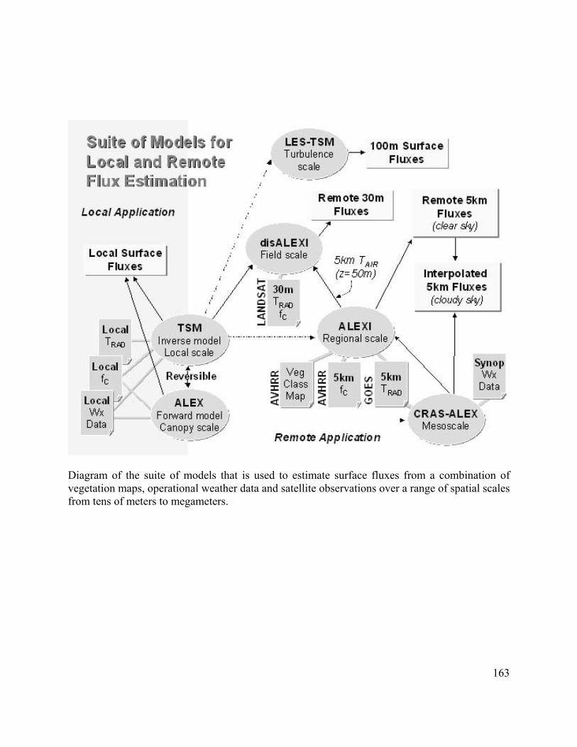
Diagram of the suite of models that is used to estimate surface fluxes from a combination of vegetation maps, operational weather data and satellite observations over a range of spatial scales from tens of meters to megameters.

163

Validation Work for SSM/IS Land Surface Temperature and Soil Moisture EDRs During SMEX02 Peggy O’Neill and Manfred Owe, Hydrological Sciences Branch / Code 974 NASA Goddard Space Flight Center, Greenbelt, MD 20771 Tom Jackson, Hydrology Laboratory, Agricultural Research Service U.S. Dept. of Agriculture, Beltsville, MD 20705 Pat Starks, Grazinglands Research Laboratory, Agricultural Research Service U.S. Dept. of Agriculture, El Reno, OK 73036 The Defense Meteorological Satellite Program’s Special Sensor Microwave Imager (SSM/I) satellites have been collecting global measurements from space for the last 15 years. With the impending launch of the latest F16 SSM/IS satellite now planned for early 2002, it is anticipated that SSM/IS will have completed its initial on-orbit checkout phase and be fully operational by the time of the SMEX02 experiment. This schedule allows the leveraging of SMEX02 activities for validation of SSM/IS soil moisture and land surface temperature Environmental Data Records (EDRs). Past research studies have demonstrated the capabilities of low frequency microwave sensors for estimation of land surface soil moisture and temperature. While papers in the refereed literature have indicated the potential of SSM/I frequencies in retrieving temperature, accurate estimates of soil moisture generally require the use of lower frequency microwave channels (preferably L band at 1.4 GHz). Because the lowest frequency on SSM/IS is at the much higher frequency of 19 GHz (1.55 cm wavelength), theoretical limitations will restrict the ability of SSM/IS to retrieve soil moisture/soil wetness to bare or lightly vegetated surfaces. The challenge for validation of the SSM/IS soil moisture EDR will be to document (in a quantified repeatable way) the accuracy of the soil moisture retrievals under specific conditions of surface vegetation and roughness. Validation Activities The main thrust of the SSM/IS validation approach will be to leverage off of NASA/USDA AMSR cal/val activities to the maximum extent possible. These activities consist of two major programs: the extensive SMEX02 soil moisture field campaign and the continuous collection of relevant data from instrument networks in four USDA watersheds across the U.S. for year-long validation. The SMEX02 soil moisture field campaign is currently scheduled for June/July, 2002, and will include aircraft overflights with AESMIR sensors at the SSM/IS channels. Since the AMSR-E frequencies of 6.6 and 10 GHz will respond to soil moisture in a deeper surface layer (~1-2 cm) than 19 GHz, most of the ground validation data will be collected at 2.5 and 5 cm depths. The relationship between soil moisture at these depths and the shallower SSM/IS sampling depth (0.3-0.5 cm) will be examined. It is likely that planned gravimetric soil moisture sampling will be augmented in limited areas to collect a 1 cm sample to supplement the SSM/IS validation.

164

Spatial scaling between point samples and the area response, which will be a part of the AMSR analysis, is directly relevant to SSM/IS because of the similar spatial extent of the SSM/IS 19 GHz and AMSR 6.6 GHz footprints.

Emissivity0

5

10

15

20

25

30

35Vo

lum

etric

Soi

l Moi

stur

e (%

)

1.4 GHz model

1.4 GHz 1992

1.4 GHz 1994

19 GHz 1992

19 GHz 1994

19 GHz model

0.7 0.8 0.9 1.0

Figure - Soil moisture-microwave relationship for Oklahoma grasslands in 1992-1994, showing the large difference in sensitivity in the microwave-soil moisture relationship between the 19 GHz SSM/I sensor and equivalent data collected at 1.4 GHz using an aircraft sensor. Long-term observations in diverse environments are needed to understand possible variations in the soil moisture – microwave relationships that arise from seasonal variations in vegetation cover and temperature. This will be accomplished by utilizing the planned upgrades under the AMSR cal/val program to in situ observations in four USDA instrumented watersheds across the U.S. (Georgia, Oklahoma, Arizona, and Idaho) to better characterize moisture and temperature conditions in the shallow surface layers. In addition, the instrument network in the Oklahoma watershed will be augmented by SMEX02 for SSM/IS temperature EDR validation work by adding fixed-mount thermal infrared thermometers to the 17 AMSR-upgraded stations in the 610 km2 Oklahoma watershed. The Oklahoma watershed currently includes 42 Micronet meteorological stations, 14 ARS SHAWMS stations (which collect 2.5 and 5 cm soil moisture and soil temperature data as part of their soil profile measurements), 2 ARM/CART stations, and 1 NRCS SCAN station. Data are recorded at 30- and 60-minute timesteps continuously year-round to provide information to assess diurnal and seasonal relationships with the satellite microwave measurements. All stations will undergo initial site-specific calibration and cross-calibration between sites for all of the soil moisture and soil temperature sensors. These calibrations will be periodically rechecked to insure data quality.

165

Use of Regional Microwave-Derived Soil Moisture in Land Data Assimilation and Atmospheric Boundary Layer Studies Peggy O’Neill, Paul Houser, Christa Peters-Lidard, Xiwu Zhan Hydrological Sciences Branch / 974, NASA Goddard Space Flight Center, Greenbelt, MD 20771 The Hydrological Sciences Branch at NASA / GSFC has a long-standing and comprehensive interest in the application of microwave remote sensing to land surface hydrology. Research within the Branch ranges from investigation of more accurate soil moisture retrieval algorithms to technology development of 2D STAR techniques to application of remote sensing variables in data assimilation and atmospheric boundary layer studies. It is anticipated that Branch members will participate in all of these areas as part of the SMEX02 experiment, especially in support of ground vegetation and soil moisture sampling. Soil Moisture Retrieval Algorithms SMEX02 will offer the opportunity to compare the accuracy of soil moisture retrieved using the standard single-channel algorithm to soil moisture retrieved using a multiple-channel approach in both a more challenging vegetated environment (Iowa) and a well-characterized low vegetation environment (Oklahoma). This work has direct bearing on future soil moisture mission planning. Land Data Assimilation The overall goal of a recently funded AMSR calibration/validation effort is (1) to quantify the accuracy and provide validation for soil moisture retrieved from AMSR-E on a variety of time scales, (2) to quantify the geographical, seasonal, and environmental sensitivities of the accuracy characteristics, and (3) to analyze the effects of these uncertainties on the predictability of the global surface water and energy balance using land surface data assimilation techniques in near real-time. The use of data assimilation methods for satellite validation is the next logical step in NASA’s ongoing efforts to understand the Earth’s land-surface and to extend NASA’s emerging observations for application to a vast array of socially-relevant land-surface issues. A nearly real-time operational land data assimilation system will be developed that will monitor the spatial-temporal AMSR soil moisture quality, so as to provide feedback to mission operators of observational problems. This system will also extend AMSR-E products in time and space to produce consistent data assimilation land surface fields that will be valuable for use in subsequent analysis and application. The in situ and airborne land surface observations from SMEX02 will be used initially as a surrogate for AMSR data in model runs of the Iowa and Oklahoma regions as a precursor to the actual AMSR cal/val field activities in 2003. For the determination of land surface biophysical parameters such as NDVI, leaf area index, land cover/use type, etc., optical remote sensing data from satellites like MODIS, ASTER, Ikonos, ETM+ and/or AVHRR will also be needed and ingested into the modeling approach. 166

Atmospheric Boundary Layer Studies Atmospheric boundary layer measurement activities planned for SMEX02 include flux towers, aircraft, lidar and ground-based sampling. The focus of the GSFC contribution to this effort will be support for ground sampling, with a special focus on soil moisture and temperature profiles, as well as LAI and soil hydraulic and thermal properties within the regional and high resolution sampling grids. This effort will support future coupled land surface-ABL modeling activities in the Iowa region.

167

An Agroecosystem Water Management Model Prediction and Calibration during SMEX02 Investigators: Z. Pan1, R. Horton1, J.H. Prueger2, D.P. Todey1, M. Segal1, and E.S. Takle1

1 Dept. of Agronomy, Iowa State University, Ames, IA 50011 2 NSTL, 2150 Pammel Drive, Ames, Iowa 50011 Contact: Zaitao Pan, 3010 Agronomy, Iowa State University, Ames, IA50011, panz@iastate.edu, Tel: (515)294-0264, Fax: (515)294-2619 Background In a project funded by the Iowa State University Agronomy Endowment Fund, we have been developing an agroecosystem water management model. This soil-plant-atmosphere coupled modeling system includes a regional climate model (MM5), soil/hydrology model (SWAT), and crop development models (CERES-Maize and CROPGRO-Soybean). The coupled modeling system will be run in forecast mode, projecting seasonal crop-available soil moisture thereby allowing evaluation of alternative cropping strategies. We have run the model for spring-summer 2001, and plan to have real-time soil moisture prediction for the growing-season 2002. The SMEX02 provides a unique opportunity for us to validate and calibrate our soil moisture forecasting model, and at the same time, our model simulation can complement SMEX02 near-surface soil moisture by providing simulation of deeper soil moisture profiles which can be useful for agricultural and hydrology applications. Experiment Objectives The overall goal of the proposed project is to use SMEX02 near-surface soil moisture observations, both in-situ and airborne, to validate and calibrate our soil moisture forecast model while dynamically interpolating observed data over the entire watershed. This will complement observed near-surface soil moisture by providing model generated root-zone data. Specifically the project has following objectives:

(1) To use SMEX02 soil moisture data to validate/calibrate our coupled model and improve model parameterization for the soil-plant-atmosphere water budget.

(2) To assimilate the soil moisture into the coupled model and generate four-dimensional soil moisture that is consistent with the observed.

(3) To dynamically generate root-zone soil moisture based on the near-surface in-situ observations via our coupled model.

(4) To evaluate effects of field-scale variability in soil wetness and energy fluxes at the surface on atmospheric boundary-layer processes, particularly convective activity.

Strategies We will adopt a multi-scale domain nesting and interdisciplinary component coupling approach. The nested regional climate model will use a GCM forecast as the initial and boundary conditions. The GCM-regional model nesting is one-way whereas within our coupled model, we

168

will have two-way interactive nesting, allowing information on finer grids to feed back to coarser grids. The planned coarsest (finest) grid spacing appropriate for this project will be about 9.0 (1.0) km. The coarse domain spans the Midwest while the fine domain, which is freely movable, covers only the Walnut Creek watershed. This triple nesting will have relatively fine grid resolution to provide detailed spatial heterogeneity while embracing large-scale dynamics of the atmosphere. Before SMEX02 starts (middle June), we will run our model to predict soil moisture distribution and temporal variation over the entire Walnut Creek watershed. The projected soil moisture will be based on the forecast precipitation, atmospheric condition, and soil water content at the time. This soil moisture forecast can also serve as a first-guess for SMEX02 participants. During the SMEX02 as the observed soil moisture is reported, we will continuously run the model while nudging the model-generated soil moisture towards the SMEX02 observation. After SMEX02, we will calibrate our model with more comprehensive and refined data. Data needed from SMEX02

• Soil and vegetation distribution • Near-surface soil moisture and temperature • Radiative properties of vegetation, LAI, CO2 concentration

Contribution to the overall SMEX02 Provide a spatio-temporal distribution of model-generated soil moisture and energy fluxes that are consistent with SMEX02 observations over the entire Walnut Creek watershed. Extend the soil moisture profile deeper into root zone by using the coupled model based on water and energy budgets, broadening future usage of SMEX02 soil moisture data by agriculture and hydrology communities. Provide an example of the SMEX02 data application in driving, validating, and calibrating land-surface schemes of climate models. If needed, we could possibly provide one or two actual soil profile sampling.

169

Spatial and Temporal Controls of Soil CO Flux 2 T.B. Parkin, USDA-ARS- National Soil Tilth Lab, Z. Senwo, Alabama A&M University T.B. Parkin, voice (515) 294-6888, Email parkin@nstl.gov Rational: Assessment of soil C storage requires precise knowledge of C inputs and losses. In agricultural systems C inputs can be estimated from crop yield data, however C losses are more difficult to estimate. A major portion of the C lost from soil occurs as CO produced from microbial action on plant material and soil organic matter. This soil-derived CO is not only a reflection of soil C degradation processes, but also represents a pool of CO that may be re-incorporated into the growing plants. Prediction of the magnitude of this process and development of an understanding of the factors controlling soil CO flux are critical to assessment of the impact of agricultural activities on soil C storage.

2

2

2

2

Hypothesis: The relationships between temperature, soil water content and soil CO flux are dependant upon landscape position.

2

Approach: Soil CO flux will be measured in transects corresponding to flight lines. Three fields along each of 3 flight lines will be sampled. In each field a stratified sampling scheme will be employed whereby three ‘replicate’ locations of each of 3 general landscape elements will be identified (Hilltop, Side-slope, and Depression), resulting in 9 locations/field. The distance between locations will depend upon specific field topography. At each landscape element location soil CO flux, soil temperature (surface and 5 cm) and soil water content (surface 5 cm - Theta probe) will be measured at 3 separate locations located 1 meter apart. Soil samples will also be collected for laboratory analysis of soil microbial enzymes (to be conducted by Z. Senwo, Alabama A & Univ.). The resulting sampling plan will result in data collected at 27 locations within each field, (81 locations on each transect : 243 locations/watershed). It is estimated that it will require a 2 person team 2 hours to sample each field, thus 3 teams of 2 people will be able to conduct sampling on the 3 transects in approximately 6 hours. Sampling will be performed twice during the experiment. Soil CO flux will be measured using soil chambers (27 cm diameter). Chambers will be placed over the soil and the chamber headspace gas recirculated through portable infrared gas analyzers to quantify increases in CO concentration over a 2 minute period. To assess temporal variations in CO flux 3 automated chambers will be placed in a single field, one on each landscape element. Automated chambers will collect soil CO flux (along with soil water content, soil temperature, air temperature, and rainfall) during 5 minute periods every hour over the duration of the experiment. These data will be used to determine diurnal responses of soil CO flux in order to account for time-of-day influences associated with the point-in-time CO transect data.

2

2

2

2

2

2

2

2

170

Data analysis: A jack-knifing procedure will be used. Data set will be split in thirds. Data from one set will be used to generate relationships between temperature, soil water content, landscape position, soil texture, and respiration. Data from the remaining 2 sets will be used as validation sets to assess accuracy of predicted CO2 fluxes. This process will be repeated 3 time, using a different model set each time. If there is consistency in the mathematical relationships over all three model sets, the remote temperature and soil water content data along with elevation and soil maps will be used to construct estimates of field and watershed CO2 fluxes. The magnitudes of these estimates will be compared with CO2 fluxes obtained by eddy correlation. It is not anticipated that soil CO2 flux and eddy correlation fluxes will be exactly comparable, since these methods measure fundamentally different processes. The chambers will only yield information on soil contribution to CO flux while Eddy correlation gives an aggregated assessment of plant and soil contributions. However, evidence in the literature suggests that recycling of soil derived CO2 may be recycled into the crop, and that this component is not accounted for by most micro-met assessments of CO2 flux measurements made above the crop canopy. Determination of the relative magnitudes of soil CO2 flux a total CO2 flux will be valuable in assessing the importance of soil-derived CO2 which has the potential to be recycled into the crop canopy. Since the transect CO2 flux will only be collected during the daytime, diurnal patterns in CO2 flux will be derived from automated chamber data. Relationships between diurnal air temperature changes and diurnal CO2 fluxes will be developed from the automated chambers, and used to estimate average daily CO2 flux at each of the transect measurement positions.

2

Data Contribution: At select locations: surface soil temperature, 5 cm soil temperature, soil water content (theta probe), soil CO2 flux, selected soil enzymes. Data requirements. Plant biomass assessments (plant height) at each soil CO2 flux location. Remote sensed soil temperature and water content. Personnel: 5 Student Hourly workers for 2 days (In addition to Parkin, Senwo, and Parkin’s technician).

171

Turbulence Mechanisms for Heat, Water and CO2 Exchange over Midwest Corn Soybean Fields. Investigators: J.H. Prueger, J.L. Hatfield, W.P. Kustas, and L.E. Hipps Contact Information: J.H. Prueger, NSTL, 2150 Pammel Drive, Ames, Iowa 50011-4419, 515-294-7694, 515-294-8125 (fax), email: prueger@nstl.gov Background: The upper Midwest region represents a major sector of production agriculture for corn and soybeans. Radiant energy partitioning into the four components of net radiation (Rn), soil heat flux (G), sensible heat (H) and latent heat (evaporation, LE) is strongly influenced by surface roughness, soil water content, soil type, and landscape position. Mechanically and thermally driven turbulence contributes to the transport of surface scalars (H, LE and CO2). Intermittent eddies of varying spatial and temporal scales can affect the energy partitioning particularly between fields having significant changes in surface roughness such as bordering soybean and corn fields. Carbon dioxide exchanges from the soil-plant atmosphere continuum are similarly affected. The vast areas of corn/soybean production represent a potential sink for C uptake. Little information is available on the role of intermittent turbulence and C uptake for Midwest cropping systems. Hypothesis: 1) Exchange of scalar fluxes of H, LE and CO2 can be related to soil type, soil water content and intermittent eddy transport events. 2) Intermittent transport events of scalars are an important component of daily energy flux exchange. Approach: Two fields, one planted in corn and the other in soybeans will be instrumented with a horizontal (north-south) transect of 4 eddy covariance systems, two in corn and two in soybeans. Both fields represent typical soil associations and topography for Midwest cropping systems. Each eddy covariance system will be comprised of a 3-Dimensioanl sonic anemometer, and an LI 7500 CO2 / H2O open path analyzer to provide measurements of the three wind components (u, v, w), water vapor density (ρv) air temperature (T) and CO2 concentration. Each system will be erected within a specific soil type and will include measurements of Rn and G. Eddy covariance instrumentation will be sampled at 10 Hz while those of Rn and G will be at 1 Hz. Radiometric temperatures (surface temperatures) will also be made at each of the sites. Data Analysis: Characteristics of the turbulent exchange related to specific flux transport events will be determined via time series analysis. This will include power spectra and co-spectra of the measured high frequency data components. These results will be used to evaluate the frequency distribution of energy containing eddies. Wavelet analysis will be used to decompose wind, water vapor, and CO2 signals to identify intermittent events during periods of non-stationarity and determine the effect on energy balance and CO2 flux computations. Data requirements: High frequency (10 Hz) measurements of the three wind components u, v, w, water vapor density, temperature, and CO2 concentration. Personnel: NSTL, Hydrology and Remote Sensing Laboratory and Utah State University scientists will supply personnel to complete these measurements.

172

173

Coupled Heat and Water Flow in Surface Soil Layers T. J. Sauer (NSTL), T. E. Ochsner, and R. Horton (ISU) Dr. Thomas J. Sauer, USDA-ARS, National Soil Tilth Laboratory, 2150 Pammel Drive, Ames, IA 50011-4420, sauer@nstl.gov, Ph. (515)294-3416, Fax (515)294-8125 Traditional surface energy balance measurement protocols involve the measurement of soil heat flux (G) using flux plates buried near the soil surface. The plates make a direct measurement of G at the depth of placement. Heat storage in the soil above the plate can be significant, often even greater in magnitude than the measured flux during daytime under sparse canopies. Heat storage in a soil layer changes not only with soil temperature but also with the soil heat capacity (C), which changes dramatically with soil water content (θ). Large changes in surface soil temperature and water content, therefore, result in rapid and substantial changes in heat storage in shallow soil layers. In order to obtain an accurate measurement of G at the soil surface, a correction for heat storage in the soil above the plate must be made. The objective of this project is to improve the accuracy of surface G measurements by developing continuous, real-time heat storage corrections for flux plate measurements using data from in-situ soil heat capacity sensors. An array of identical heat flux plates will be deployed at 0.06 m depth at 2 of the intensely monitored surface flux sites. At both locations, dual probe soil thermal property sensors will be installed in the soil above the flux plates. These sensors provide a direct and continuous estimate of soil volumetric heat capacity. Performance of this new, automated system will be compared with the traditional method of estimating C from de Vries’ equation and measured θ. Special attention will be given to intervals following rainfall when C is changing rapidly as the soil dries. Additional sensors (infrared thermometers, net radiometers, pyranometers, and quantum sensors) will be deployed to characterize the canopy microclimate, especially radiation penetration through the canopy.

174

175

Characterization of Vegetation Parameters Within a Footprint Area Of SMEX02 W. Tadesse, T. Coleman, T. Tsegaye, W. Khairy, and Bridget Sanghadasa, Alabama, A&M University, Center for Hydrology, Soil Climatology, and Remote Sensing

W. Tadesse, 256-858-4252, wtadesse@aamu.edu Rationale: Leaf area index (LAI) defined as the one-sided leaf area per unit ground area, normalized differences of the vegetation index (NDVI), and fraction of photosynthetically active radiation (fPAR) are key vegetation parameters that describe a canopy structure. Soil moisture estimation models use these parameters. Despite large developments over the past years, the main problem is still the acquisition of these vegetation parameters that are needed to input in the models. These parameters vary on a field scale and undergo rapid changes with time. In the last decade, NDVI derived from NOAA-AVHRR and Landsat Thematic Mapper (TM) have been some of the widely used sources of satellite data available to monitor the activity of vegetation from space. New sensors such as MODIS, having increased spatial resolution as well as spectral and directional properties, will provide improved land cover estimates and vegetation properties, including fPAR. Estimation of these variables from satellite and aircraft based remote sensing data require ground data for validation and testing for bias. Therefore, the objectives of this study are: (1) to measure the LAI and fPAR of soybean and corn at field scale using the AccuPAR Model PAR-80 (Decagon Devices, Inc. Pullman, WA), (2) to validate the Landsat TM, AVHRR, and MODIS derived LAI, NDVI, and fPAR parameters using field scale measurement. Hypothesis: Surface biophysical parameters (LAI, fPAR, and biomass) can be accurately estimated from satellite and aircraft remotely sensed data. Data Collection: The protocol used to measure vegetation parameters during the Southern Great Plains (SGP97) Experiments, with some modification to fit the type of crops (soybean, corn and others) at Ames, Iowa, will be utilized. Sampling locations will be coordinated with ground based flux stations and sites that will be used by Alabama A&M University (HSCaRS) scientists. The LAI and fPAR measurement will be taken on a grid from the corn and soybean field using the AccuPAR Model PAR-80 (Decagon Devices, Inc. Pullman, WA) device. Spectral reflectance measurement will be done using a hand held radiometer that will measure the incident and reflected light. NDVI will be calculated using the surface spectral measurement and satellite data. The sampling locations on the field will be recorded using differential GPS unit. The biophysical parameters measured on grid scale will be interpolated across the footprint using geostatistical kriging method. The normalized difference vegetation index (NDVI) will be derived from Landsat TM, AVHRR, and MODIS sensors and relationships will be established with the measured surface biophysical parameters (LAI, fPAR, and biomass).

176

Contribution to SMEX02: Biophysical parameters (LAI, fPAR, and NDVI) measurements obtained from the field scale will be used for watershed, and regional scale soil moisture estimation.

177

Integration of Depth Dependent Soil Moisture, Flux, and ESTAR Data to Better Characterize Soil Moisture Distribution under Corn and Soybean Fields

Teferi D. Tsegaye, Wael Khairy, Wubishet Tadesse, and Karnita Golson, Center for Hydrology, Soil Climatology, and Remote Sensing, Alabama A&M University

Teferi D. Tsegaye, voice (256) 858-4219, Email ttsegaye@aamu.edu

Soil moisture is a critical component of many regional and global climate studies. It’s spatial and temporal distribution within a field and watershed is affected by sources of the hydrological conditions and variability mostly associated with management-related factors. Furthermore, the relative significance of spatial, temporal, and management-induced sources of variation are not well known, nor are they typically accounted for in the soil moisture modeling and mapping efforts. Knowledge of their significance is nevertheless important for the development of both efficient sampling protocols and proper parameterization scenarios. The objectives of this research are: 1) evaluate the variance structure associated with soil moisture within a corn and soybean field; and 2) determine the emitting depth by correlating the near-surface soil moisture data with ground based flux and remotely sensed measurements. Hypothesis: Evaluating the relative significance of the variance structure of near-surface soil moisture improves the validation process of remotely sensed data. Sample collection: During the SMEX02 field experiment, repeated soil moisture measurements will be collected from corn and soybean fields. Soil moisture measurements will be done twice a day within-row and side-row of the row crops. Occasionally, soil moisture measurements will be done on a 100 X 100 m grid within these fields. The data collection will be coordinated with ground based flux measurements and measurements will be done at least from five soil depths including 2, 3, 4, 5, and 6 cm and in four fields (two corn and two soybean). A site-specific calibration will be performed before and after the field experiment to compare the soil moisture data collected from each field. Contribution to SMEX02 field experiment: In addition to the flux stations data, robust spatial and temporal characteristics of these data should provide important insight into soil moisture distribution under corn and soybean fields. Data collected from this study can be used to couple remotely sensed data with hydrology models and will also assist to validate remotely collected active and passive data.

178

179

Evaluation of Regression Tree Algorithm (RTA) and Artificial Neural Networks (ANNs) for Developing Pedotransfer Functions of Soil Hydraulic Parameters

Teferi D. Tsegaye1, Wael Khairy1, Wubishet Tadesse1, Karnita Golson1, Yakov Pachepsky2, and Binayak Mohanty3

1Center for Hydrology, Soil Climatology, and Remote Sensing, Alabama A&M University, 2USDA-ARS Beltsville, MD, 3Texas A&M University

Teferi D. Tsegaye, voice (256) 858-4219, Email ttsegaye@aamu.edu

Knowledge of the spatial and temporal variability of hydraulic properties at different scaling levels is essential to effectively apply many research and management tools. In addition, this will improve our ability to estimate and quantify the spatial distribution of soil moisture. Most hydrologic models that simulate soil hydrologic processes and their impacts on crop growth depend on accurate characterization of such properties. The lack of such information is often considered to be a major obstacle to effectively utilize these tools. It is generally recognized that soil hydraulic properties are affected by numerous sources of variability mostly associated with spatial, temporal, and management related factors. Soil type is considered the dominant source of variability, and parameterization is typically based on soil survey databases. We are trying to identify a set of potential algorithms to predict water retention characteristics from more readily available soil data such as texture, structure, bulk density, organic matter, and Cation Exchange Capacity (CEC). Therefore, the purpose of this study is to evaluate the relationships between soil types and their hydraulic properties at the field scale and to develop a relationship between easily measured soil properties, vegetation characteristics, and hydrologic processes for up scaling, as well as improve the performance of the hydrologic modeling.

The objective of this research is to: 1) develop hierarchical pedotransfer functions (PTFs) using soil, topography, and plant properties; 2) compare two types of PTF models (Artificial Neural Network, Regression Tree Algorithm and estimate soil hydraulic properties at different spatial scales (point and field); and 3) develop a soil database that can be used as an input for watershed or regional scale hydrology models.

Hypothesis: Successful prediction of near surface hydraulic parameters and incorporation of such parameters with existing hydrologic models will improve the model performance at the watershed and regional scales.

Sample collection and analysis: Disturbed and undisturbed soil samples will be collected from the 0-10 cm depth on a grid from two or more corn and soybean fields. The soil samples will be crushed and passed through a 2-mm sieve. The disturbed soil samples will be analyzed for particle size (texture), organic matter, Cation Exchange Capacity (CEC), and pH. Undisturbed soil cores, 7.6 cm long by 7.6 cm diameter will be collected using Uhland core sampler. The samples will be trimmed, wrapped in plastic bags, and stored in a refrigerator at 4°C prior to analysis. They will then be used for the determination of soil physical properties including saturated hydraulic conductivity, water retention, bulk density, and porosity.

180

Contribution to the SMEX02 Field Experiment: Research outcomes and the resulting database from this work will be used in the watershed and regional hydrologic modeling work.

181

14 Contacts

Name Affiliation Email

Jackson Tom HRSL tjackson@hydrolab.arsusda.gov

Bindlish Rajat HRSL bindlish@hydrolab.arsusda.gov

Cosh Mike HRSL mcosh@hydrolab.arsusda.gov

Hsu Ann HRSL hsu@hydrolab.arsusda.gov

Nijenhuis Mathieu HRSL mrnijenhuis@hydrolab.arsusda.gov

Kuijper Marijn HRSL marijnk@hydrolab.arsusda.gov

McKee Lynn HRSL lmckee@hydrolab.arsusda.gov

Dulaney Wayne HRSL wdulaney@hydrolab.arsusda.gov

Walthall Charlie HRSL cwalthal@hydrolab.arsusda.gov

Doraiswamy Paul HRSL pdoraisw@hydrolab.arsusda.gov

Crow Wade HRSL wcrow@hydrolab.arsusda.gov

Lakshmi Venkat USC vlakshmi@geol.sc.edu

Bolten John USC jbolten@geol.sc.edu

Cashion James USC Jec0913@aol.com

Srinivasan Raja USC

Schiedt Stephen USC

Famiglietti Jay UCI jfamigli@uci.edu

Berg Aaron UCI berg@uci.edu

Holl Sally UCI sholl@uci.edu

Ryu Dongrryeol UCI dryu@uci.edu

Seo Ki-Weon UCI kiweon@speer.geo.utexas.edu

Hatfield Jerry NSTL hatfield@nstl.gov

Logsdon Sally NSTL logsdon@nstl.gov

Hehr Dee NSTL hehr@nstl.gov

Kulisky Shannon NSTL kulisky@nstl.gov

Oesterriech Wolfgang NSTL oesterriech@nstl.gov

Sauer Tom NSTL sauer@nstl.gov

Parkin Tim NSTL parkin@nstl.gov

Miller Doug PSU miller@essc.psu.edu

Voortman Jon PSU jjv@essc.psu.edu

Heffelfinger Stephen PSU steveheff11@yahoo.com

Calamito Anthony PSU arc167@psu.edu

Bills Brian PSU miller@essc.psu.edu

Mohanty Binayak TAMU bmohanty@cora.tamu.edu

Jacobs Jennifer UF jjaco@ce.ufl.edu

Whitfield Brent UF

Ripo Gerard UF

Tien Calvin UF ktien@agen.ufl.edu

182

Tsegaye Teferi AAMU ttsegaye@aamu.edu

Tadesse Wubishet AAMU wtadesse@aamu.edu

Khairy Wael AAMU wkhairy@aamu.edu

Senwo Zachary AAMU zsenwo@aamu.edu

Coleman Tommy AAMU tcoleman@aamu.edu

Laymon Chip GHCC Charles.Laymon@msfc.nasa.gov

Crosson Bill GHCC Bill.Crosson@msfc.nasa.gov

Archer Frank GHCC frank.archer@msfc.nasa.gov

Limaye Ashutosh GHCC

Wood Eric Princeton efwood@h2o.Princeton.EDU

Gao Huilin Princeton huiling@Princeton.EDU

Pan Ming Princeton

Goteti Gopi Princeton

Drusch Mattias U Bonn mdrusch@uni-bonn.de

O'Neill Peggy NASA peggy@hsb.gsfc.nasa.gov

Kim Ed NASA Edward.J.Kim.1@gsfc.nasa.gov

Peters-Lidard Christa NASA cpeters@hsb.gsfc.nasa.gov

Zhan Xiwu NASA xzhan@hsb.gsfc.nasa.gov

Koike Toshio U Tokyo tkoike@hydra.t.u-tokyo.ac.jp

Pan Zaito ISU panz@iastate.edu

Prada Laura UC Berkley lparada@hydro.CE.Berkeley.EDU

Wen Jun Wageningen J.Wen@Alterra.wag-ur.nl

Manu Andrew ISU akmanu@iastate.edu

Lobl Elena UAH/MSFC elena.lobl@msfc.nasa.gov

Dinardo Steve JPL PALS steven.j.dinardo@jpl.jpl.nasa.gov

Njoku Eni JPL PALS eni.g.njoku@jpl.nasa.gov

Yeuh Simon JPL PALS simon@pals.jpl.nasa.gov

Wilson Bill JPL PALS william.j.wilson@jpl.nasa.gov

Masters Dallas CU GPS Dallas.Masters@Colorado.EDU

Cusak John NCAR C-130

Eagan Kip NCAR C-130

Genzinger Lowell NCAR C-130

Kidd Bret NCAR C-130

Nicoll George NCAR C-130

Zrubek Kurt NCAR C-130

Boynton Henry NCAR C-130

Easmunt Dave NASA P-3B deasmunt@pop800.gsfc.nasa.gov

Dykes William NASA P-3B

White Larry NASA P-3B

Yates Brian NASA P-3B

Doyle John NASA P-3B

Chase Larry NASA P-3B

Church Lee NOAA PSR

Leuskiy Vladimir NOAA PSR

183

Gasiewski Al NOAA PSR al.gasiewski@noaa.gov

Klein Marian NOAA PSR marian.klein@noaa.gov

Yevgrafov Aleksandre NOAA PSR

Zamora Bob NOAA PSR

Zavorotny Valery NOAA PSR

Le Vine David NASA ESTAR dmlevine@meneg.gsfc.nasa.gov

Gosselin Brian NASA ESTAR

Miller Chris NASA DC-8 chris.miller@dfrc.nasa.gov

Imel Dave JPL AIRSAR imel@jpl.nasa.gov

Kustas Bill HRSL bkustas@hydrolab.arsusda.gov

Russ Andy HRSL aruss@hydrolab.arsusda.gov

Prueger John NSTL prueger@nstl.gov

Hart Tim NSTL hart@nstl.gov

Neale Chris USU cneale@cc.usu.edu

Chavez Jose USU

Akasheh Osama USU

Hernandez Jairo USU

MacPherson Ian NRC-CA Ian.Macpherson@nrc.ca

Aitken John NRC-CA

Taylor Chuck NRC-CA

Depper Don NRC-CA

Desjardins Ray Agri-CA desjardins@EM.AGR.CA

Riznek Richard Agri-CA

Dow Dave Agri-CA

Albertson John Duke U. jdalbertson@virginia.edu

Williams Christopher Duke U. caw4r@virginia.edu

Emanuel Ryan Duke U.

Cahill Tony TAMU tcahill@civilmail.tamu.edu

Hipps Larry USU larry@claret.agsci.usu.edu

Brunsell Nate USU nate@gis.usu.edu

Eichinger Bill U. Iowa william-eichinger@uiowa.edu

Nichol Jennifer U. Iowa

Laszczak Steve U. Iowa

Cooper Dan LANL dccoper@lanl.gov

Archuleta John LANL jaa@lanl.gov

Fernandez Al LANL

Everett Dan LANL

Vigil Kevin LANL

Norman John U. Wisc. norman@calshp.cals.wisc.edu

Anderson Martha U. Wisc. mcanders@facstaff.wisc.edu

Diak George U. Wisc. george.diak@ssec.wisc.edu

184

15 LOGISTICS

15.1 Security

Access to fields Do not enter any field that you do not have permission to enter. Prior to the experiment all requests for field access are to be directed to Tom Jackson. Do not assume that you can use a field without permission. Requests for installations and unplanned sampling made during the experiment will not be easy to satisfy. Tracking down a landowner and getting permission can take up to a half-day of time by our most valuable people. These people will be extremely busy during the experiment. Therefore, if you think you will have specific needs that have not been addressed, you did not spend enough time planning…so learn for the next time.

• Access to field headquarters: Open 7 am until 6 pm everyday • Access to the NSTL: Restricted to USDA employees and others by prior arrangements • Access to C-130 at Des Moines airport: Restricted to aircraft personnel and others ONLY by

prior arrangement and approval • Access to the P-3B at Des Moines Airport: Restricted to aircraft personnel and others ONLY

by prior arrangement and approval 15.2 Safety

Field Hazards

There are a number of potential hazards in doing field work. The following page has some good suggestions. Common sense can avoid most problems. Remember to:

• Work in teams of two • Carry a phone • Know where you are. All roads have street signs. Make a note of your closest intersection. • Dress correctly; long pants, long sleeves, boots, hat • Contact with corn leaves can cause a skin irritation • Use sunscreen and bring fluids For medical emergencies call 911 or go to: Mary Greeley Medical Center 1111 Duff Avenue, Ames, IA 50010 Phone: 515-239-2011 For non-emergency medical problems: Adult Medicine in the McFarland Clinic 1215 Duff Avenue, Ames IA, 50010 Phone: 515-239-4431

185

186

Ticks

Ticks are flat, gray or brownish and about an eighth of an inch long. When they are filled with their victim's blood they can grow to be about a quarter of an inch around. If a tick bites you, you won't feel any pain. In fact you probably won't even know it until you find the tick clamped on tightly to your body. There may be some redness around the area, and in the case of a deer tick bite, the kind that carries Lyme Disease, a red "bulls-eye" may develop around the area. This pattern could spread over several inches of your body.

When you find a tick on you body, soak a cotton ball with alcohol and swab the tick. This will make it loosen its grip and fall off. Be patient, and don't try to pull the tick off. If you pull it off and it leaves its mouth-parts in you, you might develop an irritation around these remaining pieces of tick. You can also kill ticks on you by swabbing them with a drop of hot wax (ouch!) or fingernail polish. After you've removed the tick, wash the area with soap and water and swab it with an antiseptic such as iodine.

Ticks are very common outdoors during warm weather. When you are outdoors in fields and in the woods, wear long pants and boots. Also spray yourself before you go out with insect repellent containing DEET.

(Source:<http://kidshealth.org/cgi-bin/print_hit_bold.pl/kid/games/tick.html?ticks#first _hit>)

Drying Ovens

The temperature used for the soil drying ovens is 105oC. Touching the metal sample cans or the inside of the oven may result in burns. Use the safety gloves provided when placing cans in or removing cans from a hot oven. Vegetation drying is conducted at lower temperatures that pose no hazard.

187

15.3 Hotels

Ames, IA The following two are suggested. More info can be obtained at http://www.amescvb.com/lodging/index.asp Comfort Suites 2609 Elwood Drive Ames, IA 50010 (515) 268-8808 Fax (515) 268-8858 Information provided by Jennifer One person Mini-suite 7 or more days $50/day plus tax One person less than 7 days $55/day plus tax (also the govt. per diem rate) Additional person Add $5 per day These rooms have a refrigerator, microwave (some rooms), breakfast, pool, exercise room. http://www4.choicehotels.com/ires/en-US/html/HotelInfo?sid=OdVj.23qbiFKan.4&hotel=IA070 Howard Johnson Express Inn Hwy. 69 & Hwy. 30 Ames, IA 50010 515-232-8363 1- 800-798-8363 FAX 515-232-7751 Information from Sandy One person 7 or more days $43/day plus tax One person less than 7 days $50/day plus tax Two people 7 or more days $47/day plus tax http://www.hojo-ames.com Breakfast, pool, within walking distance of a wide range of restaurants, etc. Des Moines, IA Embassy Suites Hotel Des Moines-On The River 101 East Locust Street Des Moines, IA 50309 515-244-1700 Fax: 1-515-244-2537 NASA Group Rate for Extended Stay $67/day plus tax (govt. per diem rate) http://www.embassysuites.com/en/es/hotels/index.jhtml?ctyhocn=DSMDNES

188

Four Points by Sheraton Des Moines Airport 1810 Army Post Road Des Moines, Iowa 50325 (515) 287-6464 Fax:(515) 287-5818 One person standard room $60/night plus tax (govt. rate) http://www.starwood.com/fourpoints/index.html 15.4 Shipping Addresses

Tim Hart USDA-ARS National Soil Tilth Laboratory 2150 Pammel Drive Ames, IA 50011

189

15.5 Directions

The following map indicates one way to get to Ames from Des Moines. If coming from the airport it is more efficient to head east on Army Post Rd. to Rt. 69 North. This intersects I-235 (East) and becomes I-35 N. Maps are available at the airport near baggage claim.

190

This map shows general features of the City of Ames. All hotels have an excellent street map of Ames available for free. When coming from Des Moines, get off I-35 at Rt. 30 West and then either head North on Duff for the Ramada or South on Elwood for the Comfort Suites.

191

The location of the Field Headquarters for SMEX02 is an ARS building located on 240th St near W Ave. A photo is also shown. The All Hands meeting on June 24th will be held here.

SMEX02 Field Headquarters

15.6 Local Contacts

USDA/ARS National Soil Tilth Laboratory 2150 Pammel Drive Ames, IA 50011-4420 Jerry Hatfield John Prueger (515) 294-5723 (515) 294-7694 hatfield@nstl.gov prueger@nstl.gov

192