solar sail trajectory optimization for the solar polar imager · pdf file ·...

Solar Sail Trajectory Optimization

for the Solar Polar Imager (SPI) Mission

Bernd Dachwald∗

German Aerospace Center (DLR), 82234 Wessling, Germany

Andreas Ohndorf†

German Aerospace Center (DLR), 51170 Cologne, Germany

Bong Wie‡

Arizona State University, Tempe, AZ 85287, USA

The Solar Polar Imager (SPI) mission is one of several Sun-Earth Connection solar sailroadmap missions currently envisioned by NASA. A current SPI reference mission designis based on a 160m × 160m, 150 kg square solar sail assembly with a 250 kg spacecraft busand a scientific payload of 50 kg (450 kg total mass), having a characteristic acceleration of0.35mm/s2. Using a conservative solar sail film temperature limit of 100◦C to constrainthe solar distance (“cold” mission scenario), our transfer trajectory to the SPI target orbit(circular orbit at 0.48AU solar distance with 75 deg inclination) approaches the sun closer(to about 0.4AU solar distance) than a current reference trajectory and therefore, exploit-ing the larger solar radiation pressure, takes – even with a lower hyperbolic excess energyfor interplanetary insertion – only 6.4 instead of 6.7 years. For a higher sail temperaturelimit of 240◦C (“hot” mission scenario), the optimal transfer trajectory approaches the sunmuch closer (to about 0.22AU solar distance), resulting in an even shorter transfer dura-tion of only 4.7 years. Based on this “hot” mission scenario, we perform several missiontradeoffs to gain a deeper insight into the trade space of the SPI mission: different sailtemperature limits, different characteristic accelerations, different interplanetary insertionenergies, and different sail degradation behaviors are investigated.

I. Introduction

The Solar Polar Imager (SPI) mission is one of several Sun-Earth Connection solar sail roadmap missionscurrently envisioned by NASA. A similar solar sail mission, called Solar Polar Orbiter (SPO), is studied byESA (Ref. 1). The objective of the SPI mission is to investigate the global structure and dynamics of thesolar corona and to reveal the secrets of the solar cycle and the origins of solar activity (Refs. 2 and 3).

A current SPI reference mission design in Refs. 4 and 5 is based on a 160 m×160 m, 150 kg square solar sailassembly with a 250 kg spacecraft bus and a scientific payload of 50 kg (450 kg total mass). The characteristicthrust (max. thrust at 1 AU) of the sailcraft is Fc = 160 mN, which yields a characteristic acceleration (max.acceleration at 1AU) of ac = 0.35 mm/s2. The SPI target orbit is a heliocentric circular orbit at 0.48 AU(in 3:1 resonance with Earth) with an inclination of 75 deg (although different target inclinations have beenconsidered in various previous SPI mission studies). The current reference trajectory from Refs. 4 and 5 isshown in Fig. 1. After being placed onto an Earth-escape trajectory (with a hyperbolic excess energy ofC3 = 0.25 km2/s2) by a conventional launch vehicle such as a Delta II, the solar sail is to be deployed. Itwas first found by Wright in Refs. 6 and 7 and further examined by Sauer in Ref. 8 that the best way toperform a large inclination change with a solar sail is to first spiral inwards to a close solar distance, and

∗Scientist, German Space Operations Center, Mission Operations Section, Oberpfaffenhofen, [email protected], +49-8153-28 2772, Member AIAA, Member AAS.

†PhD Student, Institute of Space Simulation, Cologne, [email protected], +49-2203-601 2877.‡Professor, Dept. of Mechanical & Aerospace Engineering, [email protected], +1-480-965 8674, Associate Fellow AIAA.

1 of 18

American Institute of Aeronautics and Astronautics

AIAA/AAS Astrodynamics Specialist Conference and Exhibit21 - 24 August 2006, Keystone, Colorado

AIAA 2006-6177

Copyright © 2006 by the authors. Published by the American Institute of Aeronautics and Astronautics, Inc., with permission.

Mission DesignSolar Sail Trajectory Overview

Transfer Flight Path

• General Design Optimizes Thrust VectorPointing

* Cruise trajectory produces 15° heliocentricinclination change

* Thrust vector change rates are minimized

* Solar-vector to Sail-Normal-vector angle isconstrained to ≤ 45°

• 2-phase Approach Optimized for Insertionto OPS Orbit in ~6.8 years

* Cruise trajectory produces 15° heliocentricinclination change

* Cranking orbit effects ~53° inclinationchange

into the OPS orbit 60° heliocentric inclination

* Orbit trim is designed for final orbit shapingand velocity matching

Science OPS Orbit

• Designed for High Latitude Coverage with3:1 Earth Resonance

* Nodal phasing included for control of Earth-Sun-S/C angle

2012 Solar Sail Solar Polar Imager3:1 Resonance, R= 0.48 AU

75 Degrees Heliographic Inclination

ac=.35 mm/s2 CP1

Sauer 9-14-04spi340-75-1074

1 2

3

4

5Earth

DATE ∆Days

∆Years

METDays

METYears

Launch C3=0.25 km2/s2 05/24/12 0 0 0 0.000

Start of Sail Phase 06/03/12 10 0.027 10 0.027

Start of Cranking Phase 12/10/14 920 2.519 930 2.546

End of Cranking Phase 02/05/19 1518 4.156 2448 6.702

Start of Science OPS Phase 03/02/19 25 0.068 2473 6.771

0

30

60

90

120

150

180

210

240

0 200 400 600 800 1000 1200 1400 1600 1800 2000TIME FROM LAUNCH (days)

Sauer 6-1-01

CONE

CLOCK

SA

IL N

OR

MA

L C

ON

E a

nd

CL

OC

K A

NG

LE

S (

deg

)

CONE & CLOCK ANGLES vs. TIME

ALL CASES:

Nbody Trajectory Integration

10 day Initial Coast

C3 = 0.25 km2/s2

ac =0.315 mm/s2

Trajectory CharacteristicsCone and Clock

SOLARVECTOR

SAIL PLANENORMAL

NORTHECLIPTIC

CLO

CK

CONE

PLANE ⊥ TOSOLAR VECTOR

PROJECTION OFSAIL NORMAL

PROJECTION OFNORTH ECLIPTIC

• Cone Angles* 35° to 45° majority of mission

* Higher angles for short durations (post-injection,transition to cranking, pre-science orbit trim)

- Max cone angle <62°

• Clock Angles* NO abrupt changes in clock angle - actual maneuver

is a soft (2-days), single-axis maneuver of the sail normalfrom 35° below the solar vector to 35° above the solarvector. Result is to shift the projection of sail normalfrom one hemisphere to the other w.r.t. the North Ecliptic.

Figure 5. Solar sailing trajectory design of the SPI mission by Carl Sauer (Courtesy of JPL). To befurther studied by using the SSCT and/or the S5.

7 of 29

Figure 1. 3D plot of the SPI reference trajectory (credits: Carl Sauer)

then to use the large available solar radiation pressure to crank the orbit. This way, the steering strategyto reach the SPI target orbit is divided into two phases. The goal of the first phase is to spiral inwards to0.48 AU (thereby the inclination of the SPI reference trajectory is already changed by 15 deg). The goal ofthe second phase is to crank the orbit until the target inclination of 75 deg is reached. This way, the SPItarget orbit is attained after 6.7 years. Because the solar sail film temperature does not exceed 100◦C, whichis quite conservative for currently projected solar sail film materials, we have dubbed this scenario “cold”mission scenario.

We have conjectured that the SPI target orbit might be attained faster using a so-called “hot” missionscenario, where the sail spirals closer to the sun than 0.48 AU, then cranks the orbit to about 75 deg, andthen spirals outwards again. This way, the steering strategy to reach the SPI target orbit can be divided intothree phases. We have used InTrance (see Refs. 9 and 10), a method that combines artificial neural networksand evolutionary algorithms, to find a near-globally optimal trajectory. For our calculations, we have usedthe model for a non-perfectly reflecting solar sail with a sail temperature limit of 240◦C and C3 = 0 km2/s2.The resulting trajectory is shown in Fig. 2. This “hot” trajectory takes only 4.7 years.

520500450400350300

Sail Temp. [K]Arrival at target orbit(a = 0.48 AU, i = 75 deg)

Launch at Earth

Sail temperaturedoes not exceed 240°C

Figure 2. 3D trajectory plot for our “hot” mission scenario

The critical technologies required for the proposed mission include the deployment and control of a160 m × 160 m solar sail and the development of a solar sail and a micro-spacecraft bus that is able towithstand the extreme space environment at less than only 0.25 AU from the sun. A 160 m×160 m solar sailis currently not available. However, a 20 m× 20 m solar sail structure was already deployed on ground in asimulated gravity-free environment at DLR in December 1999, a 40 m×40 m solar sail is being developed by

2 of 18


NASA and industries for a possible flight-validation experiment within 10 years, and thus a 160 m × 160 msolar sail is expected to be available within about 15-20 years of a sharply pursued technology developmentprogram.

Before we describe our results for the “cold” mission scenario (section V) and for the “hot” missionscenario (section VI), we will briefly outline the employed solar sail force model for non-perfect reflection(section II), our simulation model (section III), and the used trajectory optimization methods (section IV).

II. Solar Sail Force Model

For the description of the solar radiation pressure (SRP) force exerted on a solar sail, it is convenient tointroduce two unit vectors. The first one is the sail normal vector n, which is perpendicular to the sail surfaceand always directed away from the sun. Let O = {er, et, eh} be an orthogonal right-handed coordinateframe, where er points always along the sun-spacecraft line, eh is the orbit plane normal (pointing alongthe spacecraft’s orbital angular momentum vector), and et completes the right-handed coordinate system(er × et = eh). Then in O, the direction of the sail normal vector, which describes the sail attitude, isexpressed by the pitch angle α and the clock angle δ (Fig. 3). The second unit vector is the thrust unitvector m, which points along the direction of the SRP force. Its direction is described likewise by the coneangle θ and the clock angle δ.

nm

re

te

he

αθδ

orbital plane

solar sail

sun line

plane perpendicular to th

e sun line

Figure 3. Definition of the sail normal vector and the trust normal vector

At a distance r from the sun, the SRP is

P =S0

c

(r0r

)2

= 4.563µNm2

·(r0r

)2

(1)

where S0 = 1368W/m2 is the solar constant, c is the speed of light in vacuum, and r0 = 1AU.In this paper, the standard SRP force model for non-perfect reflection from Ref. 11 by Wright is employed,

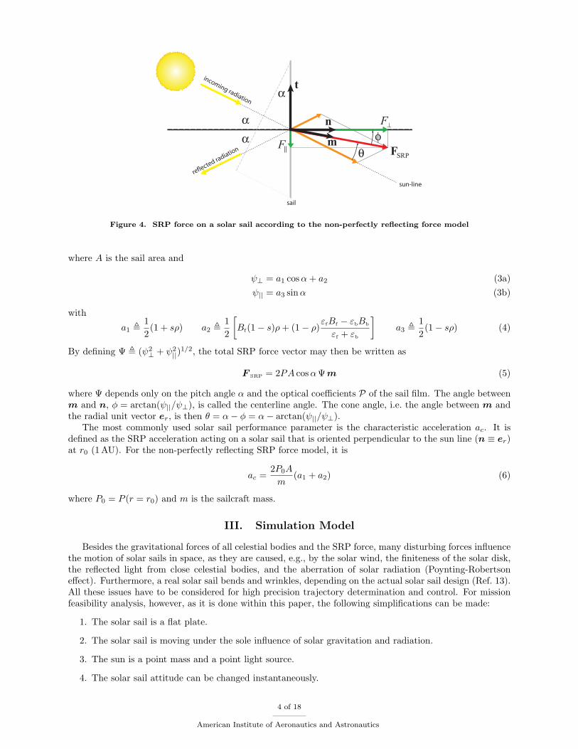
which uses the set of optical coefficients P = {ρ, s, εf , εb, Bf , Bb} to parameterize the optical characteristics ofthe sail film, where ρ is the reflection coefficient, s is the specular reflection factor, εf and εb are the emissioncoefficients of the front and back side, respectively, and Bf and Bb are the non-Lambertian coefficients ofthe front and back side, respectively, which describe the angular distribution of the emitted and the diffuselyreflected photons. According to Ref. 11, the optical coefficients for a solar sail with a highly reflectivealuminum-coated front side and a highly emissive chromium-coated back side (to keep the sail temperaturemoderate) are PAl|Cr = {ρ = 0.88, s = 0.94, εf = 0.05, εb = 0.55, Bf = 0.79, Bb = 0.55}. It can be shown(see Ref. 12) that in a sail-fixed 2D coordinate frame S = {n, t} (see Fig. 4; because of symmetry, the thirddimension is not relevant here), the SRP force exerted on the solar sail has a normal component F⊥ (alongn) and a tangential component F|| (along t) with

F⊥ = F SRP · n = 2PA cosαψ⊥ (2a)F|| = F SRP · t = −2PA cosαψ|| (2b)

3 of 18


incoming radiation

reflected radiation

sail

sun-line

αα

α

SRPF

n

t

⊥F

||F θφm

Figure 4. SRP force on a solar sail according to the non-perfectly reflecting force model

where A is the sail area and

ψ⊥ = a1 cosα+ a2 (3a)ψ|| = a3 sinα (3b)

with

a1 ,12(1 + sρ) a2 ,

12

[Bf(1− s)ρ+ (1− ρ)

εfBf − εbBb

εf + εb

]a3 ,

12(1− sρ) (4)

By defining Ψ , (ψ2⊥ + ψ2

||)1/2, the total SRP force vector may then be written as

F SRP = 2PA cosαΨm (5)

where Ψ depends only on the pitch angle α and the optical coefficients P of the sail film. The angle betweenm and n, φ = arctan(ψ||/ψ⊥), is called the centerline angle. The cone angle, i.e. the angle between m andthe radial unit vector er, is then θ = α− φ = α− arctan(ψ||/ψ⊥).

The most commonly used solar sail performance parameter is the characteristic acceleration ac. It isdefined as the SRP acceleration acting on a solar sail that is oriented perpendicular to the sun line (n ≡ er)at r0 (1AU). For the non-perfectly reflecting SRP force model, it is

ac =2P0A

m(a1 + a2) (6)

where P0 = P (r = r0) and m is the sailcraft mass.

III. Simulation Model

Besides the gravitational forces of all celestial bodies and the SRP force, many disturbing forces influencethe motion of solar sails in space, as they are caused, e.g., by the solar wind, the finiteness of the solar disk,the reflected light from close celestial bodies, and the aberration of solar radiation (Poynting-Robertsoneffect). Furthermore, a real solar sail bends and wrinkles, depending on the actual solar sail design (Ref. 13).All these issues have to be considered for high precision trajectory determination and control. For missionfeasibility analysis, however, as it is done within this paper, the following simplifications can be made:

1. The solar sail is a flat plate.

2. The solar sail is moving under the sole influence of solar gravitation and radiation.

3. The sun is a point mass and a point light source.

4. The solar sail attitude can be changed instantaneously.

4 of 18


Let the reference frame I = {ex, ey, ez} be a heliocentric inertial right-handed coordinate frame. Theequations of motion for a solar sail in the I-frame are:

r = v, v = − µ

r3r +

F SRP

m+ ad (7)

where r = (rx, ry, rz) is the solar sail position, v = (vx, vy, vz) is the solar sail velocity, µ is the sun’sgravitational parameter, and ad is the disturbing acceleration, which is – according to the simplificationsmade above – neglected within this paper.

IV. Trajectory Optimization Methods

A. Local Steering Laws

Although local steering laws (LSLs) are not a trajectory optimization method in the narrower sense, theygive the locally optimal thrust direction to change some specific osculating orbital element of the spacecraftwith a locally maximum rate. To obtain LSLs, Lagrange’s planetary equations in Gauss’ form may be used,which describe the rate of change of a body’s osculating orbital elements due to some (propulsive and/ordisturbing) acceleration. This can best be done in the orbit frame O = {er, et, eh}. According to Ref. 14,the equations for the semi-major axis a, the eccentricity e, and the inclination i can be written as

da

dt=

2a2

h(e sin far + (p/r) at) (8a)

de

dt=

1h

(p sin far + [(p+ r) cos f + re] at) (8b)

di

dt=

1hr cos(ω + f)ah (8c)

where ar, at, and ah are the acceleration components along the O-frame unit vectors, h = |h| is the orbitalangular momentum per spacecraft unit mass, ω is the argument of perihelion, f is the true anomaly, and pis the semilatus rectum of the orbit. Because Eqs. (8) can be written as

da

dt=

2a2

h

e sin fp/r

0

·

ar

at

ah

= ka · a (9a)

de

dt=

1h

p sin f(p+ r) cos f + re

0

·

ar

at

ah

= ke · a (9b)

di

dt=

1h

00

r cos(ω + f)

·

ar

at

ah

= ki · a (9c)

it is clear that to decrease (increase) the semi-major axis with a maximum rate, the thrust vector has to bealong the direction −ka (ka), which yields the local steering law La− (La+). To decrease the eccentricity witha maximum rate, the thrust vector has to be along the direction −ke (Le−), and to increase the inclinationwith a maximum rate, the thrust vector has to be along the direction ki (Li+). Unlike for other spacecraft,however, where the thrust vector can be directed into any desired direction, the SRP force vector of a solarsail is constrained to lie on a “bubble” that is directed away from the sun. Therefore, when using LSLs, theprojection of the SRP force vector onto the respective k-vector has to be maximized.

B. Evolutionary Neurocontrol

Within this paper, evolutionary neurocontrol (ENC) is used to calculate near-globally optimal trajectories.This method is based on a combination of artificial neural networks (ANNs) with evolutionary algorithms(EAs). ENC attacks low-thrust trajectory optimization problems from the perspective of artificial intelligenceand machine learning. Here, it can only be sketched how this method is used to search for optimal solar sail

5 of 18


trajectories. The reader who is interested in the details of the method is referred to Refs. 9, 10, and 15. Theproblem of searching an optimal solar sail trajectory x?[t] = (r?[t], r?[t]) – where the symbol “[t]” denotesthe time history of the preceding variable and the symbol “?” denotes its optimal value – is equivalent tothe problem of searching an optimal sail normal vector history n?[t], as it is defined by the optimal timehistory of the so-called direction unit vector d?[t], which points along the optimal thrust direction. Withinthe context of machine learning, a trajectory is regarded as the result of a sail steering strategy S that mapsthe problem relevant variables (the solar sail state x and the target state xT) onto the direction unit vector,S : {x,xT} ⊂ R12 7→ {d} ⊂ R3, from which n is calculated. This way, the problem of searching x?[t] isequivalent to the problem of searching (or learning) the optimal sail steering strategy S?. An ANN maybe used as a so-called neurocontroller (NC) to implement solar sail steering strategies. It can be regardedas a parameterized function Nπ (the network function) that is – for a fixed network topology – completelydefined by the internal parameter set π of the ANN. Therefore, each π defines a sail steering strategy Sπ.The problem of searching x?[t] is therefore equivalent to the problem of searching the optimal NC parameterset π?. EAs that work on a population of strings can be used for finding π? because π can be mapped ontoa string ξ (also called chromosome or individual). The trajectory optimization problem is solved when theoptimal chromosome ξ? is found. Figure 5 sketches the subsequent transformation of a chromosome into asolar sail trajectory. An evolutionary neurocontroller (ENC) is a NC that employs an EA for learning (orbreeding) π?. ENC was implemented within a low-thrust trajectory optimization program called InTrance,which stands for Intelligent Trajectory optimization using neurocontroller evolution. InTrance is a smartglobal trajectory optimization method that requires only the target body/state and intervals for the initialconditions (e.g., launch date, hyperbolic excess velocity, etc.) as input to find a near-globally optimaltrajectory for the specified problem. It works without an initial guess and does not require the attendanceof a trajectory optimization expert.

��

��

chromosome/individual/string ξ

=NC parameter set π

��

��

NC network function N

=sail steering strategy S

�� sail normal vector history n[t]

�� solar sail trajectory x[t]

?

?

?

Figure 5. Transformation of a chromosome into a solar sail trajectory

V. Optimization of the “Cold” Mission Scenario

Our baseline mission design foresees a non-perfectly reflecting solar sail with a characteristic accelerationof ac = 0.35 mm/s2. Although the reference mission, as it is described in Refs. 4 and 5, uses a hyperbolicexcess energy of C3 = 0.25 km2/s2 for interplanetary insertion, our baseline mission design is based onC3 = 0km2/s2 to make the different calculations better comparable.

It was first found by Wright in Refs. 6 and 7 and further examined by Sauer in Ref. 8 that the bestway to crank a solar sail orbit is to first spiral inwards to a close solar distance, and then to use the largeavailable SRP to change the inclination. Using LSLs, the strategy to attain the SPI target orbit divides thetrajectory into the following phases:

1: Spiralling inwards until the SPI target semi-major axis is reached using local steering law La− (the

6 of 18


inclination stays constant during this phase)

2A: Cranking the orbit until the SPI target inclination is reached using local steering law Li+ (the semi-major axis stays nearly constant during this phase).

2B: Circularizing the orbit until the SPI target orbit is attained using a combination of the local steeringlaws La− , La+ , and Le− (because only the inclination but not the semi-major axis stays constant whenonly Le− is applied)

The transition between phase 2A and 2B is quite indistinct. Therefore, both phases can be seen as asingle phase, phase 2. Additionally, using LSLs, the “optimization” of phase 2B is quite tricky. Therefore,when later in this paper LSLs are applied, phase 2B will be neglected, i.e. phase 2 ≡ phase 2A in this case.The transfer time is then ∆t = ∆t1 + ∆t2.

If solar sail degradation is not considered, the acceleration capability of a solar sail increases ∝ 1/r2 whengoing closer to the sun. The minimum solar distance, however, is constrained by the temperature limit ofthe sail film Tlim and the spacecraft (here, however, we consider only the temperature limit of the sail filmbut not of the spacecraft). The equilibrium temperature of the sail film is (see Ref. 12)

T =[S0

σ

1− ρ

εf + εb

(r0r

)2

cosα]1/4

(10)

where σ = 5.67 × 10−8 Wm−2K−4 is the Stefan-Boltzmann constant. Thus the sail temperature does notonly depend on the solar distance, but also on the sail attitude, T = T (r, α) (and of course on the set ofoptical parameters P). To prevent the solar sail from approaching the sun too closely, Sauer has used aminimal solar distance rlim instead of a temperature limit Tlim, probably to keep the trajectory calculationssimple. Note that a direct Tlim-constraint can be realized by constraining the pitch angle α (that is also thelight incidence angle) in a way that it cannot become smaller than the critical pitch angle, where Tlim wouldbe exceeded, i.e. α > αlim(r, Tlim). Although we could not find an explicit solar sail film temperature limitfor the SPI mission in the literature, our re-calculation of the reference mission has shown that the solar sailtemperature does not exceed 100◦C (see also Fig.7(d)). Therefore, we have chosen this temperature as thesail temperature limit for the calculations in this section, i.e. Tlim = 100◦C. Because this temperature limitis very conservative for currently projected solar sail film materials, we have dubbed this scenario “cold”mission scenario. Later, in section VI, we will also investigate “hot” mission scenarios, as they can be appliedfor higher sail temperature limits (Tlim ≥ 200◦C).

Although orbit cranking is most effective for a circular orbit, it is also important to consider ellipticorbits. Therefore, we describe the optimal orbit-cranking behavior rather by an orbit-cranking semi-majoraxis acr instead of an orbit-cranking radius. Using the direct sail temperature constraint, acr defines thetime ∆t2 that is required to crank the orbit to the required inclination. ∆t2 is influenced by two adverseeffects, leading to an optimal orbit-cranking semi-major axis acr,opt(Tlim) where the inclination change rate∆i/∆t is maximal and thus ∆t2 is minimal, as it can be seen from Fig. 6. For acr > acr,opt, the inclination

0.34 0.36 0.38 0.4 0.42 0.44 0.46 0.48 0.50.034

0.036

0.038

0.04

0.042

0.044

0.046

acr [AU]

∆i /

∆t [d

eg/d

ay]

Figure 6. “Cold” mission scenario: Inclination change rate over orbit-cranking semi-major axis (Tlim = 100◦C,ac = 0.35 mm/s2), circular orbit

7 of 18


change takes longer than for acr,opt because of the lower SRP. For acr < acr,opt, the inclination change alsotakes longer than for acr,opt because of the (inefficiently) large critical pitch angle αlim that is required to keepT < Tlim. Thus ∆t2 = ∆t2(Tlim). It can be seen from Fig. 6 that acr,opt(Tlim = 100◦C) = 0.422 AU where∆i/∆t(Tlim = 100◦C, ac = 0.35 mm/s2) = 0.0444 deg/day.

We have used three different methods to calculate solar sail trajectories for the “cold” mission scenario:

1. LSLs: The local steering laws La− and Li+ were applied as described above.

2. InTrance + LSL: InTrance was used to calculate a near-globally optimal transfer to a circular0.48 AU-orbit with an inclination of 15 deg (as for the reference mission described in Refs. 4 and 5),and then the local steering law Li+ was applied.

3. InTrance: InTrance was used to calculate a near-globally optimal transfer to the SPI target orbit.

Table 1 shows the obtained results and Fig. 7 shows the variation of the inclination, the semi-major axis,and the sail film temperature along the trajectory.

Table 1. “Cold” mission scenario results

Method Transfer duration Tmax ∆a ∆e ∆i[days] [years] [◦C]

[10−4AU

][10−2] [deg]

LSLs 2658 7.28 95 0.2 5.8 0.0InTrance + LSL 2513 6.88 91 2.6 7.2 0.0InTrance 2334 6.39 100 3.1 0.9 0.1

0 500 1000 1500 2000 25000

10

20

30

40

50

60

70

t [days]

i [de

g]

LSLsInTrance + LSLInTrance

(a) Inclination over flight time, i(t)

0 500 1000 1500 2000 25000

0.1

0.2

0.3

0.4

0.5

0.6

0.7

0.8

0.9

1

t [days]

a [A

U]


(b) Semi-major axis over flight time, a(t)

0 0.1 0.2 0.3 0.4 0.5 0.6 0.7 0.8 0.9 10

10

20

30

40

50

60

70

a [AU]

i [de

g]


(c) Inclination over semi-major axis, i(a)

0 500 1000 1500 2000 2500

−20

0

20

40

60

80

100

120

t [days]

T [°

C]


(d) Sail film temperature over flight time, T (t)

Figure 7. “Cold” mission scenario: Comparison of different solutions

Looking at Table 1 and Fig. 7, one can clearly see that using local steering laws and patching togetherthe solutions of phase 1 and 2 yields a suboptimal solution. The (InTrance+LSL)-trajectory is 145 days

8 of 18


faster than the LSL-trajectory. It proves that the optimal trajectory has a smooth transition between thetwo phases, changing the inclination also during phase 1, whenever the sailcraft is close to the nodes. TheInTrance-solution approaches the sun much closer than 0.48 AU, as can be seen from Figs. 7(b) and 7(c). Theclosest solar distance is only 0.407 AU (we note that this is smaller than acr,opt). This closer solar distanceyields a higher inclination change rate so that the target inclination is reached earlier (without exceedingthe sail temperature limit of 100◦C). This result shows that faster trajectories can be obtained for a givensail temperature limit Tlim, if not a minimum solar distance rlim but Tlim is used directly as a constraint.

VI. Optimization of a Faster “Hot” Mission Scenario

Because a sail temperature limit of 100◦C is quite conservative for currently projected solar sail films, wenow release this constraint and use a sail temperature limit of 240◦C. This way, the sail can approach thesun closer. It can be seen from Fig. 8 that acr,opt(Tlim = 240◦C) = 0.22 AU where ∆i/∆t(Tlim = 240◦C, ac =0.35 mm/s2) = 0.1145 deg/day and thus much higher than for Tlim = 100◦C.

0.2 0.25 0.3 0.35 0.4 0.45 0.50.03

0.04

0.05

0.06

0.07

0.08

0.09

0.1

0.11

0.12

acr [AU]

∆i /

∆t [d

eg/d

ay]

Figure 8. “Hot” mission scenario: Inclination change rate over orbit-cranking semi-major axis (Tlim = 240◦C,ac = 0.35 mm/s2), circular orbit

Using local steering laws, the “hot” scenario to attain the SPI target orbit divides the trajectory into thefollowing phases:

A: Spiralling inwards until the optimum solar distance for cranking the orbit is reached using local steeringlaw La− (the inclination stays constant during this phase)

B: Cranking the orbit until the SPI target inclination is reached using local steering law Li+ (the semi-major axis stays nearly constant during this phase).

C1: Spiralling outwards until the SPI target semi-major is reached using local steering law La+ (the incli-nation stays constant during this phase)

C2: Circularizing the orbit until the SPI target orbit is attained using a combination of the local steeringlaws La− , La+ and Le− (because only the inclination but not the semi-major axis stays constant whenonly Le− is applied)

The transition between phase C1 and C2 is quite indistinct. Therefore, both phases can be seen as asingle phase, phase C. Additionally, using LSLs, the “optimization” of phase C2 is quite tricky. Therefore,phase C2 will be neglected when LSLs are applied, i.e. phase C ≡ phase C1 in this case. The transfer timeis then ∆t = ∆tA + ∆tB + ∆tC.

We have used two different methods to calculate solar sail trajectories for the “hot” mission scenario:

1. LSLs: The local steering laws La− , Li+ , and La+ were applied as described above.

2. InTrance: InTrance was used to calculate a near-globally optimal transfer to the SPI target orbit.

9 of 18


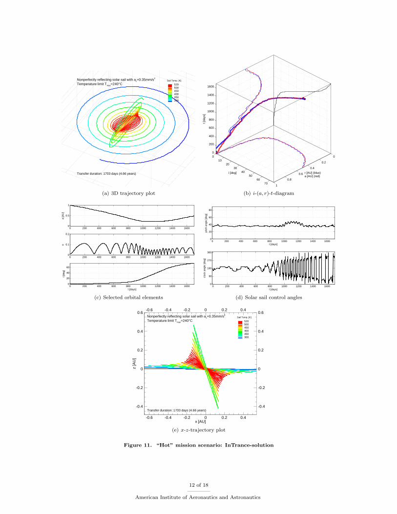
Table 2 shows the obtained results and Fig. 9 shows the variation of the inclination, the semi-major axis,and the sail film temperature along the trajectory. Figure 10 shows the trajectory, the variation of selectedorbital elements, and the control angles for the LSL-solution, while Fig. 11 shows the same for the InTrance-solution. Looking at the relatively large final eccentricity in Fig. 10(c), one can see that phase C2 has beenomitted. Due to the poor local search behavior of InTrance (note that the control angles are determined by aneural network!), some “noise” remains in the control angles (Fig. 11(d)). Further fine-tuning of the solutionwith a local trajectory optimization method might therefore yield a marginally shorter (but probably alsoless robust) trajectory.

Table 2. “Hot” mission scenario results

Method Transfer duration Tmax ∆a ∆e ∆i[days] [years] [◦C]

[10−4AU

][10−2] [deg]

LSLs 1771.5 4.85 240 0.1 8.5 0.1InTrance 1703.0 4.66 240 1.2 0.4 0.1

0 200 400 600 800 1000 1200 1400 16000

10

20

30

40

50

60

70

t [days]

i [de

g]

LSLsInTrance


0 200 400 600 800 1000 1200 1400 16000

0.1

0.2

0.3

0.4

0.5

0.6

0.7

0.8

0.9

1

t [days]

a [A

U]

LSLsInTrance

(b) Semi-major axis over flight time, a(t)

0 0.1 0.2 0.3 0.4 0.5 0.6 0.7 0.8 0.9 10

10

20

30

40

50

60

70

a [AU]

i [de

g]

LSLsInTrance

(c) Inclination over semi-major axis, i(a)

0 200 400 600 800 1000 1200 1400 1600

0

50

100

150

200

250

t [days]

T [°

C]

LSLsInTrance

(d) Sail film temperature over flight time, T (t)

Figure 9. “Hot” mission scenario: Comparison of the LSL-solution with the InTrance-solution

10 of 18


x [AU]0

0.5y [AU]

-0.5 0 0.5 1

520500450400350300

Transfer duration: 1771.5 days (4.85 years)

Sail Temp. [K]

Nonperfectly reflecting solar sail with ac=0.35mm/s2

Temperature limit Tmax=240°C

(a) 3D trajectory plot

0

0.2

0.4

0.6

0.8

1

010

2030

4050

6070

0

200

400

600

800

1000

1200

1400

1600

r [AU] (blue)a [AU] (red)

i [deg]

t [da

ys]

(b) i-(a, r)-t-diagram

0 200 400 600 800 1000 1200 1400 16000

0.5

1

a [A

U]

0 200 400 600 800 1000 1200 1400 16000

0.1

0.2

e

0 200 400 600 800 1000 1200 1400 16000

20

40

60

i [de

g]

t [days]

(c) Selected orbital elements

0 200 400 600 800 1000 1200 1400 16000

20

40

60

80

pitc

h an

gle

[deg

]

t [days]

0 200 400 600 800 1000 1200 1400 16000

90

180

270

360

cloc

k an

gle

[deg

]

t [days]

(d) Solar sail control angles

Figure 10. “Hot” mission scenario: LSL-solution

11 of 18


520500450400350300

Transfer duration: 1703 days (4.66 years)

Sail Temp. [K]Nonperfectly reflecting solar sail with ac=0.35mm/s2


(a) 3D trajectory plot

0

0.2

0.4

0.6

0.8

1

010

2030

4050

6070

0

200

400

600

800

1000

1200

1400

1600

r [AU] (blue)a [AU] (red)

i [deg]

t [da

ys]

(b) i-(a, r)-t-diagram

0 200 400 600 800 1000 1200 1400 16000

0.5

1

a [A

U]

0 200 400 600 800 1000 1200 1400 16000

0.1

0.2

e

0 200 400 600 800 1000 1200 1400 16000

20

40

60

i [de

g]

t [days]

(c) Selected orbital elements

0 200 400 600 800 1000 1200 1400 16000

20

40

60

80

pitc

h an

gle

[deg

]

t [days]

0 200 400 600 800 1000 1200 1400 16000

90

180

270

360

cloc

k an

gle

[deg

]

t [days]

(d) Solar sail control angles

x [AU]

z[A

U]

-0.6

-0.6

-0.4

-0.4

-0.2

-0.2

0

0

0.2

0.2

0.4

0.4

-0.4 -0.4

-0.2 -0.2

0 0

0.2 0.2

0.4 0.4

0.6 0.6

520500450400350300

Transfer duration: 1703 days (4.66 years)

Sail Temp. [K]Nonperfectly reflecting solar sail with ac=0.35mm/s2


(e) x-z-trajectory plot

Figure 11. “Hot” mission scenario: InTrance-solution

12 of 18


A. Variation of Mission Design Parameters

1. Variation of the Sail Temperature Limit

In this section, the influence of the sail temperature limit Tlim on the SPI mission performance is investigated.Figure 12 shows for a circular orbit, how the inclination change rate varies with the orbit-cranking semi-major axis for different sail temperature limits, i.e. (∆i/∆t)(Tlim, acr). For 200◦C ≤ Tlim ≤ 260◦C, theoptimal orbit-cranking semi-major axis can be approximated with an error of less than 2% by

acr,opt ≈ 1.4805− 0.23 · ln(Tlim) (11)

where acr,opt = acr,opt1 AU and Tlim = Tlim

1◦C . The maximum inclination change rate can be approximated with anerror of less than 2% by

(∆i/∆t)max ≈ 0.0113 · a−1.53cr,opt (12)

where (∆i/∆t)max = (∆i/∆t)max1 deg/day .

0.2 0.25 0.3 0.35 0.4 0.45 0.50.03

0.04

0.05

0.06

0.07

0.08

0.09

0.1

0.11

0.12

0.13

acr [AU]

∆i /

∆t [d

eg/d

ay]

Tlim = 100°C

Tlim = 150°C

Tlim = 200°C

Tlim = 220°C

Tlim = 240°C

Tlim = 260°C

Figure 12. Inclination change rate over orbit-cranking semi-major axis for different sail temperature limits(ac = 0.35 mm/s2), circular orbit

We have used InTrance to optimize the SPI trajectory for different solar sail temperature limits (200◦C ≤Tlim ≤ 260◦C). The results are shown in Table 3 and Fig. 13. Figure 13(b) shows that InTrance matchesthe optimal orbit-cranking semi-major axes shown in Fig. 12 very closely. The transfer duration can beapproximated with an error of less than 1% by

∆t(acr,opt) = ∆tA(acr,opt) +75 deg

(∆i/∆t)max(acr,opt)+ ∆tC(acr,opt)− ζ (13)

or

∆t(acr,opt) =(235 + 826 (1− acr,opt)

)+

750.0113 · a−1.53

cr,opt

+(30 + 771 (0.48− acr,opt)

)− 87

= 1374− 1597 acr,opt +75

0.0113 · a−1.53cr,opt

Table 3. Variation of Tlim (ac = 0.35 mm/s2, C3 = 0km2/s2)

Tlim acr,opt (∆i/∆t)max Transfer duration[◦C] [AU] [deg/day] [days] [years]200 0.260 0.0899 1793 4.90220 0.236 0.1015 1736 4.75240 0.220 0.1145 1679 4.60260 0.205 0.1291 1644 4.50

13 of 18


0 200 400 600 800 1000 1200 1400 16000

10

20

30

40

50

60

70

t [days]

i [de

g]

Tlim = 200°C

Tlim = 220°C

Tlim = 240°C

Tlim = 260°C


0 0.1 0.2 0.3 0.4 0.5 0.6 0.7 0.8 0.9 10

10

20

30

40

50

60

70

a [AU]

i [de

g]

Tlim = 200°C

Tlim = 220°C

Tlim = 240°C

Tlim = 260°C

(b) Inclination over semi-major axis, i(a)

Figure 13. Variation of Tlim (ac = 0.35 mm/s2, C3 = 0km2/s2)

60 65 70 75 80 85 904

4.5

5

5.5

iT [deg]

∆ t [

yr]

Tlim = 200°C

Tlim = 220°C

Tlim = 240°C

Tlim = 260°C

Figure 14. Approximate transfer times for different target inclinations (ac = 0.35 mm/s2, C3 = 0km2/s2)

where ∆t = ∆t1 day and ζ = 87days is approximately the time that can be saved by the near-globally optimal

steering strategy with respect to a LSL-based steering strategy. Figure 14 shows the approximate transfertimes for different target inclinations iT and temperature limits, as they can be obtained by using

∆t(Tlim, iT) = ∆t(Tlim, 75 deg) +iT − 75 deg(∆i/∆t)max

(14)

Note that the transfer time for 240◦C is shorter than in Table 2 because of different accuracy requirementsfor the fulfilment of the final constraint. In Table 2, ∆a ≤ 10 000 km, ∆e ≤ 0.01, and ∆i ≤ 0.3 deg wasrequired, while here only ∆a ≤ 50 000 km, ∆e ≤ 0.01, and ∆i ≤ 0.5 deg was required to speed up thetrajectory optimization process.

2. Variation of the Characteristic Acceleration

Next, we have investigated the influence of the characteristic acceleration ac on the mission performance. Wehave used InTrance to optimize the SPI trajectory for different characteristic accelerations (0.25 mm/s2 ≤ac ≤ 0.4 mm/s2). The results are shown in Table 4 and Fig. 15. Figure 15(b) shows that the optimal orbitcranking semi-major axis is independent of ac. The transfer duration can be approximated with an error ofless than 1% by

∆t ≈ 593/ac (15)

14 of 18


Table 4. Variation of ac (Tlim = 240◦C, C3 = 0km2/s2)

ac ∆t[mm/s2

][days] [years]

0.25 2365 6.480.3 1967 5.390.35 1679 4.600.4 1497 4.10

0 500 1000 1500 20000

10

20

30

40

50

60

70

t [days]

i [de

g]

ac = 0.25 mm/s2

ac = 0.30 mm/s2

ac = 0.35 mm/s2

ac = 0.40 mm/s2


0 0.1 0.2 0.3 0.4 0.5 0.6 0.7 0.8 0.9 10

10

20

30

40

50

60

70

a [AU]

i [de

g]

ac = 0.25 mm/s2

ac = 0.30 mm/s2

ac = 0.35 mm/s2

ac = 0.40 mm/s2


Figure 15. Variation of ac (Tlim = 240◦C, C3 = 0km2/s2)

3. Variation of the Hyperbolic Excess Energy for Interplanetary Insertion

Next, we have investigated the influence of the hyperbolic excess energy C3 (or hyperbolic excess velocityv3 =

√C3) on the mission performance. We have used InTrance to optimize the spiralling-in to a 0.48 AU

circular orbit for different hyperbolic excess energies (0 km2/s2 ≤ C3 ≤ 4 km2/s2). The transfer time ∆tsthat can be saved by injecting the sailcraft with some hyperbolic excess velocity is shown in Fig. 16.

0 0.25 0.5 1 1.25 1.5 1.75 20.750

20

40

60

80

100

120

140

160

v3 [km/s]

∆ t s

aved

[day

s]

Figure 16. Variation of C3 (Tlim = 240◦C, ac = 0.35 mm/s2)

Thus a C3 of 0.25 km2/s2 makes the reference trajectory from Refs. 4 and 5 about 50 days (0.13 years)faster w.r.t. to the C3 of 0 km2/s2 that is used in our mission design.

15 of 18


B. Solar Sail Degradation

To investigate the effects of optical degradation of the sail film, as it is expected in the extreme spaceenvironment close to the sun, we apply here the parametric model developed in Ref. 16. In this parametricmodel the optical parameters p are assumed to depend on the cumulated solar radiation dose (SRD) Σ(t)on the sail:

p(t)p0

=

(1 + de−λΣ(t)

)/ (1 + d) for p ∈ {ρ, s}

1 + d(1− e−λΣ(t)

)for p = εf

1 for p ∈ {εb, Bf , Bb}

(16)

The (dimensionless) SRD is

Σ(t) =Σ(t)Σ0

=(r20

∫ t

t0

cosαr2

dt′)/

1 yr (17)

with Σ0 , S0 · 1 yr = 1368 W/m2 · 1 yr = 15.768 TJ/m2 being the annual SRD on a surface perpendicular tothe sun at 1AU. The degradation constant λ is related to the “half life solar radiation dose” Σ (Σ = Σ ⇒p = p0+p∞

2 ) via

λ =ln 2Σ

(18)

The degradation factor d defines the end-of-life values p∞ of the optical parameters:

ρ∞ =ρ0

1 + ds∞ =

s01 + d

εf∞ = (1 + d)εf0

εb∞ = εb0 Bf∞ = Bf0 Bb∞ = Bb0

Figure 17 and Table 5 show the results for different degradation factors 0 ≤ d ≤ 0.2, assuming a half lifeSRD of 25S0 ·1 yr = 394 TJ/m2.

0 200 400 600 800 1000 1200 1400 1600 18000

10

20

30

40

50

60

70

t [days]

i [de

g]

d = 0.0d = 0.05d = 0.1d = 0.2


0 0.1 0.2 0.3 0.4 0.5 0.6 0.7 0.8 0.9 10

10

20

30

40

50

60

70

a [AU]

i [de

g]

d = 0.0d = 0.05d = 0.1d = 0.2


Figure 17. Different optical degradation factors (Tlim = 240◦C, ac = 0.35 mm/s2, C3 = 0km2/s2)

Table 5. Transfer times for different degradation factors (Tlim = 240◦C, ac = 0.35 mm/s2, C3 = 0km2/s2)

Degradation ∆tfactor [days] [years]0.0 1679 4.600.05 1742 4.770.1 1810 4.960.2 1945 5.33

16 of 18


For 0 ≤ d ≤ 0.2, the transfer time can be approximated with an error of less than 0.2% by

∆t ≈ 1677 + 1335 · d (19)

The main degradation effect can be seen from Fig. 17(a), which shows that ∆i/∆t becomes smaller withincreasing SRD. Figure 17(b) shows that for larger degradation factors it is favorable to crank the orbitfurther away from the sun than it would be optimal without degradation. Because optical degradation isan important factor for this mission, and because the real degradation behavior of solar sails in the spaceenvironment is to a considerable degree unknown, extensive ground and in-space tests are required prior tothis mission.

VII. Conclusions

A current SPI reference mission design for the Solar Polar Imager (SPI) mission is based on a 160 m× 160 m, 450 kg square solar sail spacecraft, having a characteristic acceleration of 0.35mm/s2. To attainthe SPI target orbit (circular orbit at 0.48 AU solar distance with 75 deg inclination), the current referencetrajectory spirals inwards to 0.48 AU and then cranks the orbit to 75 deg. Because for this scenario the solarsail film temperature stays colder than 100◦C, which is a conservative value, we call this a “cold” missionscenario. Using this temperature limit as a direct constraint for trajectory optimization instead of a solardistance limit, we have found a faster transfer trajectory than the reference trajectory that approaches thesun closer (to about 0.4 AU solar distance) an thus better exploits the solar radiation pressure, which islarger closer to the sun.

For higher sail temperature limits of 200-260◦C, i.e. “hot” mission scenarios, we have found that theoptimal transfer trajectories approach the sun even closer (to about 0.20-0.26 AU solar distance, dependingon the sail temperature limit), resulting in even shorter transfer durations. Based on this “hot” missionscenario, we have also performed tradeoffs for the sail temperature limit, the characteristic acceleration andthe interplanetary insertion energy to gain a deeper insight into the trade space of the SPI mission and tohelp the designer of such a mission to estimate the required transfer time.

By investigating different solar sail degradation behaviors, we have also found that the mission perfor-mance might be considerably affected by optical degradation of the sail surface, as it is expected in theextreme space environment close to the sun. Because the real degradation behavior of solar sails is to aconsiderable degree unknown, ground and in-space tests should be done prior to this mission.

Acknowledgements

The work described in this paper was funded in part by the In-Space Propulsion Technology Program,which is managed by NASA’s Science Mission Directorate in Washington, D.C., and implemented by the In-Space Propulsion Technology Office at Marshall Space Flight Center in Huntsville, Alabama. The programobjective is to develop in-space propulsion technologies that can enable or benefit near and mid-term NASAspace science missions by significantly reducing cost, mass or travel times.

References

1Macdonald, M., Hughes, G., McInnes, C., Lyngvi, A., Falkner, P., and Atzei, A., “Solar Polar Orbiter: A Solar SailTechnology Reference Study,” Journal of Spacecraft and Rockets, accepted.

2NASA’s Sun-Earth Connection Division Website, http://sec.gsfc.nasa.gov.3“Sun-Solar System Connection. Science and Technology Roadmap 2005 - 2035,” NASA publication, NASA, 2005.4Wie, B., Thomas, S., Paluszek, M., and Murphy, D., “Propellantless AOCS Design for a 160-m, 450-kg Sailcraft of the

Solar Polar Imager Mission,” 41st AIAA/ASME/SAE/ASEE Joint Propulsion Conference and Exhibit, Tucson, USA, July2005, AIAA Paper 2005-3928.

5Wie, B., “Thrust Vector Control of Solar Sail Spacecraft,” AIAA Guidance, Navigation, and Control Conference, SanFrancisco, USA, August 2005, AIAA Paper 2005-6086.

6Wright, J., “Solar Sailing – Evaluation of Concept and Potential,” Tech. rep., Battelle Columbus Laboratories, Columbus,Ohio, March 1976, BMI-NLVP-TM-74-3.

7Wright, J. and Warmke, J., “Solar Sail Mission Applications,” AIAA/AAS Astrodynamics Conference, San Diego, USA,August 18-20, 1976, AIAA Paper 76-808.

8Sauer, C., “A Comparison of Solar Sail and Ion Drive Trajectories for a Halley’s Comet Rendezvous Mission,” AAS/AIAAAstrodynamics Conference, Jackson, USA, September 1977, AAS Paper 77-104.

17 of 18


http://sec.gsfc.nasa.gov

9Dachwald, B., Low-Thrust Trajectory Optimization and Interplanetary Mission Analysis Using Evolutionary Neurocon-trol , Doctoral thesis, Universitat der Bundeswehr Munchen; Fakultat fur Luft- und Raumfahrttechnik, 2004.

10Dachwald, B., “Optimization of Interplanetary Solar Sailcraft Trajectories Using Evolutionary Neurocontrol,” Journal ofGuidance, Control, and Dynamics, Vol. 27, No. 1, pp. 66–72.

11Wright, J., Space Sailing, Gordon and Breach Science Publishers, Philadelphia, 1992.12McInnes, C., Solar Sailing. Technology, Dynamics and Mission Applications, Springer–Praxis Series in Space Science

and Technology, Springer–Praxis, Berlin, Heidelberg, New York, Chicester, 1999.13Garbe, G., Wie, B., Murphy, D., Ewing, A., Lichodziejewski, L., Derbes, B., Campbell, B., Wang, J., Taleghani, B.,

Canfield, S., Beard, J., and Peddieson, J., “Solar Sail Propulsion Technology Development,” Recent Advances in GossamerSpacecraft , edited by C. Jenkins, Vol. 212 of Progress in Astronautics and Aeronautics, American Institute of Aeronautics andAstronautics, Reston, 2006, pp. 191–261.

14Battin, R., An Introduction to the Mathematics and Methods of Astrodynamics, AIAA Education Series, AmericanInstitute of Aeronautics and Astronautics, Reston, revised ed., 1999.

15Dachwald, B., “Optimization of Very-Low-Thrust Trajectories Using Evolutionary Neurocontrol,” Acta Astronautica,Vol. 57, No. 2-8, 2005, pp. 175–185.

16Dachwald, B., Mengali, G., Quarta, A., and Macdonald, M., “Parametric Model and Optimal Control of Solar Sails withOptical Degradation,” Journal of Guidance, Control, and Dynamics, accepted.

18 of 18


solar sail trajectory optimization for the solar polar imager · pdf file ·...

Documents