Solar Tracker ECE 476, Spring 2005

Toby Peterson (tp62@cornell.edu)

Justin Rice (jkr25@cornell.edu) Jeff Valane (jmv33@cornell.edu)

Introduction: We set out to build a solar tracker. The tracker uses two Nema 23 bipolar stepper motors to rotate 2 photovoltaic cells around the altitude and azimuth axes. We have three tracking algorithms to track the sun. The first moves the PV panel in little squares in spherical coordinates, finds the point on the square with the best voltage, and moves there, then starts over. The second moves in a little square, finds the voltage gradient, and uses that to decide where to move. The third uses the second strategy to find 5 or 6 good points spread 1hour apart, uses a multivariable, nonlinear, least-squares fit to find its latitude, the day of the year, the time of day, and then predicts where the sun will be next. It will use this equation for a few repositions, and then check to make sure it’s right using the second algorithm. In moving the PV panel, our stepper motors ramp up to speed in order to prevent overshoot and jerk/rattling. To prevent the stepper motors from rattling around and drawing current when not being sent a signal, we use two relays to cut their current. The buttons of the STK500 allow the user to calibrate the tracker and choose the tracking algorithm. High Level Design: Rationale, Idea Sources: It was pretty clear from the start that our prototype solar tracker wouldn’t be self powering, but our rationale was that we could build a low level prototype with only a couple solar panels that would have many of the same interesting design problems as building a full sized, self powering solar tracker. As for idea-sources, we knew that there were solar trackers in existence, but that they weren’t commonly installed or used because the of the large added expense(instead of paying for a microcontroller and motors, you can just buy more solar panels) for the small payback in power output. We had no idea how they worked, but suspected they were programmed according to their location and the date, and thus were relatively stupid machines. We decided we wanted to build a two axis solar tracker and start with a basic tracking function and then progressively try and make it smarter and more efficient the best we could. We decided not to use the ‘put an led in a tube and use it as a light sensor’ method, because we thought the tracking problem would be more interesting without it. We used stepper motors instead of other types of actuation because we needed a holding torque to keep the PV panels in place when no power was being applied. Background Math: Basics: The math behind the mechanical and electrical functioning of the tracker itself is pretty basic. The solar panel rotates around two axes, the vertical and the horizontal. The angle about the vertical axis is called the azimuthal angle and is 0 at due south and becomes positive as you start to point east. The angle about the horizontal axis is called the altitude and is 0 level to the

horizon and becomes positive as you point towards the sky. In the program all calculations are done in radians, but for clarity in this discussion we will use degrees. The stepper motors we obtained are NEMA size 23 with 200 steps per revolution, or 200 steps per 360 degrees. For the azimuth stepper motor, we used a gear ratio of 48:10 to decrease the motion ratio to 960 steps per revolution. For the altitude stepper motor, we used a gear ratio of 4:1 to decrease the motion ratio to 800 steps per revolution. However, these super high motion ratios were only necessary to produce enough torque to move the heavy solar panels, and the backlash in our gears was large enough so that we only stepped the motors in 4 step increments(making it 240steps per revolution for the azimuth and 200 steps per revolution for the altitude). The different gear problems were no problem initially, but made some of the later math something of a pain with all the conversions. For those fuzzy on their conservation of energy

P=Tw Where P is power, T is torque, and w is angular velocity. So for constant power from the stepper motor, a gear ratio of 4 caused the angular velocity to decrease by a factor of 4, and thus the torque to increase by a factor of 4. This change in torque was true for both the holding torque and the transient torque of the stepper motors(the holding torque is the torque necessary to break the stepper lose when no voltage is being applied, the transient torque is the torque being applied while the stepper is moving). Solar Math: For a photovoltaic(PV) cell, the voltage produced is proportional to the power of the light hitting the surface. If the PV cell is not orthogonal to the light source, the voltage decreases with the projected area, or the cosine of the angle. See diagram:

light

Vo

V0cosθ

θ

Figure 1:

Later we will use this information for tracking. Also, if we have two voltages and the angle between them, we can use this information to find the angle to the sun in the following way: The Gradient Method We have two voltages, V1 and V2 and they are an angle φ apart, and we also have Vo which is the voltage the PV would get if it were perpendicular to the light source(see figure2 below). We want to find out the angle θ between the location of V1 and V0.

We can say

V1=V0cos(θ) (1) And

V2=V0cos(θ-φ)=V0cosθcosφ+V0sinθsinφ=V1cosφ+V0sinθsinφ (2) Rearranging, we have

(V2-V1cosφ)/sinφ=V0sinθ (3) inserting (1) into (3) we get

(V2-V1cosφ)/sinφ=V1tanθ (4) and rearranging, we get: arctan((V2-V1cosφ)/V1sinφ)=θ (5) So if we know V2 and V1 and φ, we can calculate where we want to go, θ. This method is used in the algorithm TrackD(), to be discussed later. For a really smart solar tracker we need the equation of the sun in our coordinates. As found by Szokolay[1996] and Carruthers, et al [1990](and found on the Square One website in the appendix), it is: t = (2 * pi * ((day - 1) / 365.0))

V0

θ

φ

V2

V1

Figure 2

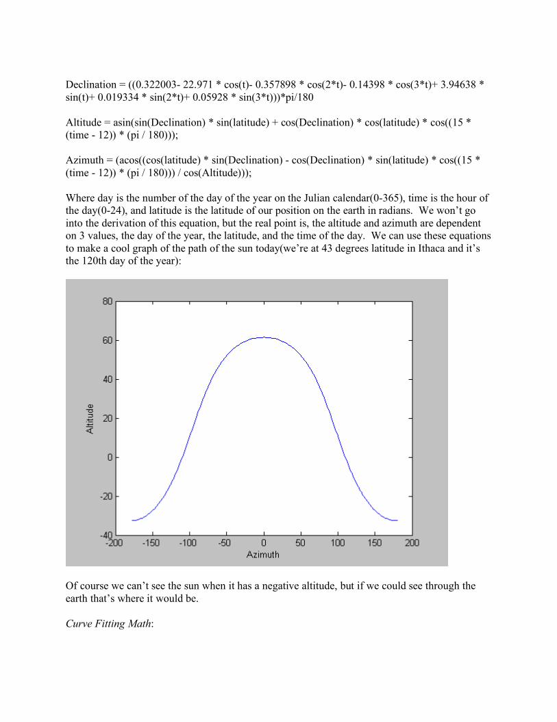
Declination = ((0.322003- 22.971 * cos(t)- 0.357898 * cos(2*t)- 0.14398 * cos(3*t)+ 3.94638 * sin(t)+ 0.019334 * sin(2*t)+ 0.05928 * sin(3*t)))*pi/180 Altitude = asin(sin(Declination) * sin(latitude) + cos(Declination) * cos(latitude) * cos((15 * (time - 12)) * (pi / 180))); Azimuth = (acos((cos(latitude) * sin(Declination) - cos(Declination) * sin(latitude) * cos((15 * (time - 12)) * (pi / 180))) / cos(Altitude))); Where day is the number of the day of the year on the Julian calendar(0-365), time is the hour of the day(0-24), and latitude is the latitude of our position on the earth in radians. We won’t go into the derivation of this equation, but the real point is, the altitude and azimuth are dependent on 3 values, the day of the year, the latitude, and the time of the day. We can use these equations to make a cool graph of the path of the sun today(we’re at 43 degrees latitude in Ithaca and it’s the 120th day of the year):

Of course we can’t see the sun when it has a negative altitude, but if we could see through the earth that’s where it would be. Curve Fitting Math:

This part is also a bit hairy. For a sophisticated solar tracker, we would want it to be more autonomous, to be able to track the sun without having to know exactly where it is, and without searching for the sun all the time and wasting extra energy. For this, it is necessary to use some of the sun data you have to figure out your position and time, and to predict where the sun will be next. The way we’ll do this is by curve fitting an equation to our data, and the specific method we’ll use is the least-squares method modified for a multivariable, nonlinear equation. So lets say we have a few data points that we think are linear and we want to fit them to a straight line. Our data might look something like this:

0

2

4

6

8

10

12

14

16

18

20

0 2 4 6 8 10 12 14 Now we know the equation for a line is y=mx+b, where m and b are unknowns. From just looking at the graph we can probably guess that b, the y-intercept, is somewhere between 0 and 5, and m, the slope, is somewhere between 0 and 2. One way of figuring out the line of best fit is to search through a bunch of values of m and b, try them in the equation, and figure out the square of the error. Which ever values of m and b have the lowest error squared are the ones we’ll use. So we could try every value of m from 0 to 2 in increments of .02 and every value of b from 0 to 5 in increments of 0.05, but this would be 10,000 attempts, and would take quite a bit of computing time. A much more frugal way to do it and end up with the same accuracy would be to try every value of m from 0 to 2 in increments of .2 and every value of b from 0 to 5 in .5 increments, find the best value, and then refine our search. We could then do a search in m of range .4 in increments of 0.02 around the best previous value, and a search in b of range 1 in increments of 0.05 around the best previous value of b, and find the best values. This will give us the same accuracy as our calculation before, but instead of taking 10,000 attempts, we’ll do it in only 500(100 for the first run, 400 for the second) which will take us 20 times less computing.

We could then keep refining our search if we desired to get more accurate values. We use a modified version of this method in TrackC(), discussed later on. Logical Structure From a high-level perspective, the design is very simple. The microcontroller has two inputs; the buttons and the ADC. There are only two outputs; to control each motor. The interface functions as follows:

(1) Turn it on. (2) Press a button to calibrate… wait for this to complete. (3) Press a button to choose a tracking mode. From now on, no button input is accepted. (4) The device will then enter its main loop, running the tracking mode over and over.

The three tracking modes are designed to reuse as much code as possible. Each is built on MoveCircle(), MoveStep(), RecordData(), and Reposition(). This is covered in more detail below, but this is a basic overview. The simplest tracking mode (TrackE) simply runs MoveCircle() and Reposition()s to the best point repeatedly. TrackD does the same thing, but tries to calculate things a little bit more intelligently. TrackC, on the other hand, is an entirely different beast. First, it uses TrackD() to gather good data, then extrapolates the sun’s path, and manually moves the solar tracker itself. It also takes about eight hours to run. Hardware/Software Tradeoffs We had to make some compromises in our design to make things work properly. For example, the relays are there because the motors grind (but don’t move) when received “no” signal from the microcontroller. Additionally, we were not able to run the motors as fast as we’d like, simply because the software can’t keep up. Another factor in this is that the PV panels take a few milliseconds to respond, as is discussed later. We also had to try not to move the motors too quickly, as they have a tendency to rattle and move unpredictably. So, we had to add in a fairly significant amount of code to support variable speeds and acceleration. Standards Conformance The key portion of our circuit is the use of PV solar panels. There is one key IEEE standard for safe operation of the equipment, but this is intended for a much more massive distributions than ours.

IEEE 929 requires the PV unit to disconnect from the utility system during a power outage. The PV system can reconnect to the utility system only after power has been restored for at least 5 minutes. Operating an electrical system during an outage is called “islanding.” Personal injury can occur if the “island generator” feeds a utility system that is being repaired and assumed disconnected from all energy sources. The need for standard interconnection requirements for small to medium PV systems was the driving force behind IEEE 929. With IEEE 929 in place, inverter designers can produce standardized equipment, thus lowering PV system costs. Before IEEE 929, many utilities required 200W and larger customer generators to comply with the expensive interconnection requirements established for very large (>100MW) generators. These large steam or engine driven generators can cause severe disturbances to a utility grid if not controlled by utility requirements, whereas a small PV inverter, properly designed, can almost instantly disconnect itself from the grid. There are many other IEEE standards for recommended practice for use of the solar cells, but once again these are in much greater scale than our implementation. Patents and Copyrights As far as existing copyrights/patents, these are all for specific designs of trackers. Since we created everything ourselves and did not develop it for wide scale deployment, our tracker was unique to all existing tracker patents. Program/Hardware design: Program Details The code is very straightforward. Probably the toughest part was simply maximizing code reuse and sanity, which made things much easier in the end. Following is a summary of the various functions used. Our lowest level functions are MoveStep(), AtLimit(), Pause(), RecordData() and HandleButtons(). AtLimit() checks the global position of the solar panel and returns a 1 or a 0 depending on if the panel is hitting the angle limit that is set to prevent it from hitting things. Pause() waits for a certain amount of time, then sends a pulse to the relays to turn them back on so that the stepper motors can move again. We use Pause() in the code to keep the motors quite between repositions. RecordData() uses the ADC to record voltage input from the PV panel. It also keeps track of the position of the highest local voltage, and records specially the values of the data at corners of the square used in TrackD() and TrackE(). MoveStep() just sends pulses to the appropriate stepper motor in the appropriate direction and then keeps track of the local and global coordinates, it also uses AtLimit() to make sure it doesn’t go past the angle limits.

HandleButtons() just scans for buttonpushs. If a button is pushed it will call the tracking function associated with that button.

Our higher level functions are Calibrate(), Reposition(), MoveCircle(), and TrackSun(). We also have ResetTracker() which just resets a bunch of variables that include the local position of the tracker(reset to 0,0) and the best position. Reposition() uses MoveStep() to make the variables ‘local_position’ x and y equal to ‘best_position’ x and y. This is used after data has been taken to relocate the PV panel to the best position available. MoveCircle() moves the PV in a little circle(really a square) in spherical coordinates with a radius of the user’s choosing. It uses RecordData() at each position on the circle for use in Reposition() in the tracking functions. It then returns the PV back to it’s original local position. Calibrate() is used right after the tracker is turned on. It tilts the PV panel to altitude=45degrees, pans the azimuth 180 degrees one way then 360 degrees the other, finds the best azimuth value, and repositions there. It then pans the full reaches of altitude angles within its limits as defined by AtLimit(), finds the best altitude, and repositions there. This is just a basic function to initially find the light source to be tracked.

Our highest level functions are the tracking functions, trackE(), trackD(), and trackC(). TrackE() is pretty simple, and stands for Elementary tracking. It just uses MoveCircle() to move the PV in a circle and record data, and then it just Repositions to the position on the circle with the best voltage, and does another MoveCircle(). This is very slow for trying to find the sun, and very inefficient too, since it has to do so many MoveCircles() to get anywhere.

TrackD() stands for Derivative tracking, because it uses the voltage gradient from the data from MoveCircle to figure out where the light source is, even if it’s far away from the best coordinates in MoveCircle and then repositions over there. It does this using the four corner points from the square in MoveCircle in the gradient method described in Background Math. TrackD() uses this method for both the altitude and the azimuth, using V1 and V2 values from the corners of the square from MoveCircle(). It then uses Reposition() to move the PV to the predicted best position. TrackC() stands for Track cool, and is the best algorithm we came up with. It uses TrackD() once per hour to find 5 data points of altitude and azimuth, and then uses a curve fitting method to find the time of day, the day of year, and the latitude, and to predict where to move next. The method that TrackC() uses to find the equation is similar to the one described in the Background Math section, except instead of searching for two variables, m and b, it searches through three variables, time, date, and latitude, and instead of fitting the data to a straight line, it fits it to the curve of the sun, as also discussed in the Background Math section. Due to its very slow nature, we cannot demo TrackC(), but we can show cool graphs we made using Matlab simulations and provide the scripts for the reader to demo for his/herself. The script, ‘solarpath.m’ allows the user to enter values of latitude, the day of the year, the starting hour of the day, and the number

of data points desired, and the program will spit out a matrix, ‘datafortest’, with values of altitude and azimuth for that day. If the user then runs ‘solarfind4.m’, the program will take ‘datafortest’, and use the curve fitting method described to find the latitude, the starting time of day for the data, and create a graph comparing the curve-fit equation to the real one, and showing the next 5 predicted data points in magenta. It will also spit out the error, in degrees, of these data points. Here is an example output: error = 0.3411 0.0562 0.6285 0.2831 0.9551 0.5291 1.3136 0.8056 1.6888 1.1294 Where the first column is the azimuth error in degrees and the second column is the altitude error in degrees.

(time moves from right to left along the line)

Where the data from solarpath are in red and the predicted data points are in magenta. (note, this graph was generated using a latitude of 43 degrees, a starting time of 10am, and day of 60). Our error shows us that for the next 4 repositions we should be within 1 degree of accuracy. But really, cos(1 degree)=0.9998476, so being off by 1 degree will only result in a decrease in voltage of about 0.02%, and cos(10 degrees)=.9848, so we really have a lot of leeway for being wrong without much loss in power.

The method by which the algorithm works is quite clever. The user enters values of: klimit: the maximum number of times the program will zoom in. the counter k keeps

track of the number of times that this has happened alpha: which is the number of grid cells that the search domain will be

divided into residuallimit: the sum of the squared error is called the residual error. The user can set this

value, and if by dumb luck the residual error is below this limit, the code will end without doing a lot of extra refinement. The residual limit is checked after an entire loop of searching, before k is augmented.

So the user specifies these values, and the program uses a similar method to that we discussed in the background math section: it will search latitude values of 0-90 degrees, day values of 0-365, and time values of 0-24. It will then compute the error for each of these possible combinations against the data-points given to it from solarpath(), find the combination of values with the least squared error. It will then zoom in on the best value, and do another search with a smaller search area and a finer grid. It will continue doing this until it has zoomed in klimit times, or the least squared error is less than residuallimit. To demonstrate this last point, here is the graph of the residual error as a function of k for the demonstrated case above, only with the residual limit set to 0.000000015:

So we can see that the more we zoom in, the lower our residual error gets, just as we would expect.(Note, this much precision is complete useless, normally a good residual limit to do is about 0.0015 or so, for this demonstration it was set really low to show the convergence of the error)

The angle errors for this calculation are ridiculously low: error = 0.0280 0.0167 0.0422 0.0269 0.0580 0.0385 0.0753 0.0520 0.0931 0.0682 We should note here that it will not be possible for our actual tracker to ever know the altitude of the sun to within 0.06 degrees 5 hours away, as there are all kinds of hardware inaccuracies that prevent it from taking exact data, or from ever pointing at the sun at such an exact angle. The program will also print out the number of gridpoints that it searched in order to find the solution. For our first demonstration, with residuallimit=0.0015, which generated our azimuth altitude graph above, 900 grid points were checked, and for our second demonstration with the residual limit set at 0.000000015 only 1800 grid points were checked. 900 grid points may seem like a lot, but considering that the mega32 has 1 hour to run it before it needs to move again, there is certainly plenty of time. As implemented in our c-code for the mega32, TrackC() uses the TrackD() algorithm to find 5 data points, 1 hour apart, then uses the curve fitting algorithm to find the next 3 points, then uses TrackD() again to find another 5 hourly points, etc. Hardware Details The hardware design in our circuit consisted of three main portions: the driver circuitry for the stepper motors, the relay circuitry, and the voltage control circuitry. The stepper motors are complex electromotive devices that require precise timing control (such that the current is pushed and pulled through the two internal coils of the stepper motor at the precise time to drive the motor in the correct direction. Since we were unsure how much torque would be required to move the PV panels we opted on 2 separate 2A 12VDC stepper motors. The immediate concern was how to drive the stepper motors. Luckily, there are prepackaged devices that take in much simpler signals and take care of the driving signals for the stepper motors. For our stepper motor drivers we chose the LMD18245 which have the capability of producing a signal with enough driving force to accommodate up to 55VDC at 3A (more than enough for our stepper motors). The driver circuitry for the motors were much more complex than I’m used to so our circuitry for that consisted of an exact replica of the recommended circuit provided in the data sheet. A copy of this schematic can be found in the Appendix. After setting up the stepper motors we found out that the stepper motors would not run. After multiple hours spent debugging we found out that the 2 additional wires on the stepper motor, which were supposed to be used for half stepping the motor (a feature we didn’t need so we ignored) needed to be connected for the motor to operate. Then after getting the motors to step properly we found that when we were not giving the drivers any driving signals (when we didn’t

want it to move) on occasion the motor would continue to produce a very irritating humming noise. We found out that the 2 additional wires on the stepper motor when disconnected would stop the noise (possible a result of inductive coupling between the two coils causing resonating). Regardless, the noise was irritating and was undoubtedly sucking up power so we needed a solution. I sampled two automotive relays from Tyco Electronics and applied 12V to one side of the switching terminals and connected the other half to the Drain of a MOSFET. I connected the source to ground and hooked the gate up to an output pin of the MCU. The relays I procured allowed for a constant connection between 2 terminals when off and that connection to be broken when power was applied. Thus whenever the MCU drove the gate of the MOSFET high it would provide a path to ground for the relay causing it to break the connection between the two wires attached to its terminals. Thus, I had a way to keep the 2 half-step wires connected while stepping but to disconnect them when staying stationary through the use of only one additional port pin. This circuitry is available in the Appendix. Lastly was the voltage control circuitry. This was pretty simple in that it used the fact that there is a voltage regulator on the STK-500. Ideally the STK-500 is supposed to be powered with 9VDC but here we have 12-15V powering the stepper motor drivers and some 12V-5V-voltage regulators that I had sampled at the beginning of the project. I decided that it would suffice to apply 10V to the STK 500 and so I connected two 5V regulators in series to produce the 10V. Things we tried which did not work. Originally we had planned on trying to make the solar tracker self powering, but this turned out to be entirely infeasible. As we were limited by our budget constraints, we had a pretty cheap mechanical setup, without bearings and such, that just barely allowed us to maneuver the 2 solar panels we used without exceeding the torque capabilities of the stepper motors. Had we carefully machined everything and used expensive needle bearings, we probably could have carried a few more solar panels, but still not nearly enough to power the energy thirsty 12V, 2.3amp stepper motors. We decided that to try for self-powering would be more of a project in mechanical design, and thus abandoned it. We also at one point planned on powering the stepper motors and STK-500 off of a motorcycle 12V battery, but this plan also went awry when we discovered that we drained the battery too fast to really use it. Results of the Design Speed of execution The user can program in different values for different accuracies in the curve fitting algorithm, and different radii for the circle in TrackD() and TrackE() to achieve different tracking speed levels if so desired. However, the fact remains that the sun moves pretty slow, and so as long as none of the algorithms take more than about an hour to work, there shouldn’t be any trouble. As for the speed that everything actually moves at, as discussed above, we accelerated the stepper motors wherever we could to make the calibration function and reposition functions

happen as fast as possible, but this was mainly because we were tired of waiting for them to finish during debugging and because we thought that making them accelerate would look and sound cool(it does). The addition of acceleration also stopped the solar tracker from vibrating so much, because the mass of the PV panels was slowly ramped up to speed, instead of just stopped and started from full speed Accuracy As discussed in the background math section, the voltage produced by the PV panels is proportional to the cosine of the angle away from perpendicular to the light source. So if the PV is 1 degree from perpendicular, we have 99.98% of the maximum possible voltage, if it is 10 degrees from perpendicular, we have 98.5% of the maximum value. With two PV panels, the maximum value we could get out of the ADC was approximately 180, using all the bits, with a minimum of 0 in the complete dark, so we see that the best sensing resolution we can really get is about

arcos(179/180)=~ 6 degrees In addition, due to wear on the inside bearing surface of the large azimuth gear from extensive testing, there ended up being a little wobble in the solar panel during motion, adding to the inaccuracy. Because of this inaccuracy, we made the program so that if the calculated reposition was less than 15 steps, it would pause for 10 seconds and wait for the light to move some more before doing any more searching. We also worried about the inaccuracy of the PV panels themselves. In our quest for speed, we accelerated the calibration() function to the point where it was stepping every 20 milliseconds. However, we checked the transient response of the PV panels using the oscilloscope, and found that the voltage level didn’t really hit steady state until about 40 milliseconds after the light was turned on(as we see in the picture below), so we had to slow Calibration() down significantly to record accurate data. This is why Reposition(), which takes no data, moves so much faster than Calibration().

The TrackC() function, as already discussed, has much much better accuracy than is possible from the mechanical and electrical systems, and is relatively insignificant in comparison. As for the timing, the accuracy of the crystal(0.05%) is orders of magnitude better than that for the electrical, mechanical, or software systems, and is very insignificant in comparison. Design Safety There are essentially three features of our design that are designed for safety. First, the wires are fairly securely taped together, so that they don’t get caught in the stepper motor gears. The other features are software-based. We keep track of the solar panels’ position, and prevent them from going too far in any direction. This means that they won’t hit the frame, or pull the wires too far. We also added a feature to make the motors accelerate up to full speed, which reduces the amount of rattling and possibility for damage. Interference with other people's designs (e.g. cpu noise, RF, interference)

While the rattling of our solar tracker is somewhat obnoxious, it doesn’t cause any RF interference or anything like that, and we haven’t actually had any complaints about the noise, outside of our own group. Usability Since our solar tracker has very little user interface, we don’t run into many usability problems. The user is only required to push two buttons, once each, and we have given them labels to make identification easier. Unfortunately we have no well thought out design to allow severely visually impaired or otherwise handicapped people to use our design, but Braille labels could easily be produced for the buttons if necessary. Conclusions: Analysis of Design We ended up being pretty satisfied with our end result. The tracker follows light fairly well in its different modes. It avoids breaking the PV panels or pulling the wires out by having motion limits. It gradually accelerates from 0 to a max speed and then down again without out any overshoot or slippage. It uses transistors and relays to prevent the stepper motors from vibrating and making unnecessary noise when not in use. It would have been better if the tracker was self-powering, but given the difficulty in such a task, we accept the failure easily. As it is, it is necessary to level the solar panel and point the altitude stepper motor due south before calibration; if we could do it again, it would be cool to have an integrated compass and inclination sensor so that this could be done automatically during calibration. It would also have been interesting to program TrackC() to work for more than a day at a time; at the end of the day it could move to the best position for when the sun rises the next morning, but this is pretty trivial. Intellectual Property We did not reuse code or someone else’s design, use code in the public domain, reverse-engineer a design, or sign any non-disclosure agreements to get sample parts. There don’t really seem to be any patent opportunities for our project, as there are lots of solar trackers out there, most of which work much better than ours and actually power themselves. Also, we haven’t come up with any non-obvious original ideas. Ethical Considerations Our solar tracker doesn’t seem to have any ethical problems. In completing this project we are complying with the 1st, 3rd, 5th, 7th, and 9th points in the IEEE code of ethics: We comply with the first point in that we have frankly discussed any safety or environmental dangers associated with our design, and accept responsibility for them. The third point requires us to be honest with respect to our claims and estimates of performance, and we have had an

honest discussion of the accuracy limits of our design. We believe that by designing our project and putting our design and report on the web, we have improved the understanding of technology for anyone who reads our report or views our webpage, thus complying with the fifth point. We are honoring the seventh point by properly crediting our sources for the equation of motion of the sun. We are abiding by the 9th point in that our product is not meant to harm anyone, nor could it foreseeably without a lot of effort (see safety considerations). Legal Considerations We did not use a transmitter, and thus have nothing to do with the FCC. In addition, our device breaks no other laws that we know of. Appendix with commented code See website.

Schematics:

Power relay circuit

Appendix with cost information: Budget: STK500+MCU $15 Power supply $5 2 Applied Motion Nema 23 Stepper motors $7.95*2= $15.90 4 LMD18245T motor drivers sampled 2 48 tooth gears $2.90*2= $5.80 1 12 tooth gear $0.55 1 10 tooth gear $0.99 bunch of bolts found bunch of washers found bunch of nuts found aluminum blocks and sheet found 2 PV panels found/borrowed 2 steel shafts for gears found 2 relays found 1 set screw found 1 white board $6.00 1 bread board found bunch of capacitors found/sampled bunch of resistors found/sampled 2 tip transistors $0.39*2= $0.78 __________________ sum total $50.02 points deduction: (($50.02-$50.00)*.316)2 = 4*10-5 points Tasks Justin Rice: Mechanical design and fabrication Wiring of motors, drivers, PV Tracking algorithms Software debugging Toby Peterson: Lead software designer Website Circuit debugging Jeff Valane: Breadboard layout

Circuit design General electrical tasks

Data sheets: http://www.national.com/pf/LM/LMD18245.html

Vendor websites: Transistors: http://www.hosfelt.com/en-us/dept_167.html Gears: http://www.probelay.com/0409250126.shtml (note, 48 tooth gear is sold out and is no longer on the website, but we have the receipt) Motor Drivers: http://www.national.com/pf/LM/LMD18245.html Motors: http://www.alltronics.com/stepper_motors.htm Washers, bolts, screws, aluminum, steel shafts, nuts, set screw: http://www.mae.cornell.edu/maelab/EMERSON.htm Relays: http://fsae.mae.cornell.edu/ Background/Reference websites: http://www.squ1.com/index.php?http://www.squ1.com/solar/sun-path-diagrams.html