A

cd1aecd©

K

1

tcbictimo5gue

c

0d

Journal of Power Sources 161 (2006) 628–639

Solid-state diffusion limitations on pulse operation ofa lithium ion cell for hybrid electric vehicles

Kandler Smith, Chao-Yang Wang ∗Electrochemical Engine Center (ECEC), and Department of Mechanical Engineering, The Pennsylvania State University,

University Park, PA 16802, USA

Received 21 December 2005; received in revised form 15 March 2006; accepted 28 March 2006Available online 11 May 2006

bstract

A 1D model based on physical and electrochemical processes of a lithium ion cell is used to describe constant current and hybrid pulse powerharacterization (HPPC) data from a 6 Ah cell designed for hybrid electric vehicle (HEV) application. An approximate solution method for theiffusion of lithium ions within active material particles is formulated using the finite element method and implemented in the previously developedD electrochemical model as an explicit difference equation. Reaction current distribution and redistribution processes occurring during dischargend current interrupt, respectively, are driven by gradients in equilibrium potential that arise due to solid diffusion limitations. The model is

xtrapolated to predict voltage response at discharge rates up to 40 C where end of discharge is caused by negative electrode active material surfaceoncentrations near depletion. Simple expressions are derived from an analytical solution to describe solid-state diffusion limited current for shorturation, high-rate pulses.

2006 Elsevier B.V. All rights reserved.

icle; T

tsttofo

umrbvtS

eywords: Lithium ion battery; Electrochemical modeling; Hybrid electric veh

. Introduction

Hybrid electric vehicles (HEVs) use a battery as a high-rateransient power source cycled about a relatively fixed state-of-harge (SOC). In the literature however, most fundamentallyased battery models focus on predicting energy available at var-ous constant current discharge rates beginning from the fullyharged state [1–3]. Cell phone, laptop, and electric vehicle bat-eries are typically discharged over some hours and it is commonn the literature to term discharge rates of only 4 C (four times the

anufacturer’s nominal one hour Ah rating, lasting on the orderf 15 min) as “high-rate”. In contrast, Hitachi states that their.5 Ah HEV cell can sustain 40 C discharge from 50% SOC forreater than 5 s. Phenomenological models capable of capturingltra-high-rate transient behavior are needed to understand and

stablish the operating limitations of HEV cells.

In the mathematical modeling of HEV cells, equivalent cir-uit models are often employed [4–7] and validated in either

∗ Corresponding author. Tel.: +1 814 863 4762; fax: +1 814 863 4848.E-mail address: cxw31@psu.edu (C.-Y. Wang).

mccwam[

378-7753/$ – see front matter © 2006 Elsevier B.V. All rights reserved.oi:10.1016/j.jpowsour.2006.03.050

ransient; Solid-state diffusion

he time or frequency domain [8–10]. While the simplicity ofuch models makes them attractive, unlike fundamental modelshey provide no insight into underlying physical cell limita-ions. Many good works do exist in the fundamental modelingf lithium ion cells, though validated models are only availableor cell phone, laptop, and electric vehicle batteries. We brieflyutline some of those works.

Doyle et al. [11] developed a 1D model of the lithium ion cellsing porous electrode and concentrated solution theories. Theodel is general enough to adopt a wide range of active mate-

ials and electrolyte solutions with variable properties and haseen applied in various studies [1,2,12–14]. In [1], Doyle et al.alidated the model against constant current data (with rates upo 4 C) from similar cells of three different electrode thicknesses.olid and electrolyte phase mass transport properties were esti-ated to fit measured data, and in particular, the solid diffusion

oefficient for LixC6 (Ds− = 3.9 × 10−10 cm2 s−1) was chosen toapture rate dependent end of discharge. Interfacial resistance

as used as an adjustable parameter to improve the model’s fit

cross the three cell designs. More recently, the 1D isothermalodel was validated against a 525 mAh Sony cell phone battery

2]. The authors used a large Bruggeman exponent correcting for

K. Smith, C.-Y. Wang / Journal of Power Sources 161 (2006) 628–639 629

Nomenclature

as active surface area per electrode unit volume(cm2 cm−3)

A electrode plate area (cm2)A state matrix in linear state variable model state

equationB input matrix in linear state variable model state

equationc concentration of lithium in a phase (mol cm−3)C state matrix in linear state variable model output

equationD diffusion coefficient of lithium species (cm2 s−1)D input matrix in linear state variable model output

equationF Faraday’s constant (96,487 C mol−1)i0 exchange current density of an electrode reaction

(A cm−2)I applied current (A)jLi reaction current resulting in production or con-

sumption of Li (A cm−3)L width (cm)p Bruggeman exponentQ capacity (A s)r radial coordinate (cm)R universal gas constant (8.3143 J mol−1 K−1)Rf film resistance on an electrode surface (� cm2)Rs radius of solid active material particles (cm)RSEI solid/electrolyte interfacial flim resistance

(� cm2)s Laplace variable (rad s−1)t time (s)t0+ transference number of lithium ion with respect

to the velocity of solventT absolute temperature (K)Ts time step (s)U open-circuit potential of an electrode reaction (V)x negative electrode solid phase stoichiometry and

spatial coordinate (cm)y positive electrode solid phase stoichiometry

Greek symbolαa, αc anodic and cathodic transfer coefficients for an

electrode reactionδ penetration depth (cm)ε volume fraction or porosity of a phaseη surface overpotential of an electrode reaction (V)κ conductivity of an electrolyte (S cm−1)κD diffusional conductivity of a species (A cm−1)σ conductivity of solid active materials in an elec-

trode (S cm−1)τ dimensionless time for solid-state diffusionφ volume-averaged electrical potential in a phase

(V)ω frequency (rad s−1)

Subscriptse electrolyte phases solid phases,avg average, or bulk solid phases,e solid phase at solid/electrolyte interfaces,max solid phase theoretical maximum limitsep separator region− negative electrode region+ positive electrode region

Superscriptseff effective

tcttdi

vdpcebsldt∼

drbasebciwatce

iucfeo

Li lithium species

ortuosity in the negative electrode (p = 3.3) leading to the con-lusion that the battery was electrolyte phase limited. Thoughhe model successfully predicted end of discharge for rates upo 3 C, the voltage response during the first minutes of dischargeid not match and was found to be sensitive to values chosen fornterfacial resistances.

While the majority of the modeling literature is devoted tooltage prediction during quasi-steady state constant currentischarge and charge, we note several discussions of transienthenomena relevant to HEV cells. Neglecting effects of con-entration dependent properties (that generally change mod-stly with time), the three transient processes occurring in aattery are double-layer capacitance, electrolyte phase diffu-ion, and solid phase diffusion. Due to the facile kinetics ofithium ion cells, Ong and Newman [15] demonstrated thatouble-layer effects occur on the millisecond time scale and canhus be neglected for current pulses with frequency less than

100 Hz.Unlike double-layer capacitance, electrolyte and solid phase

iffusion both influence low-frequency voltage response and theelative importance of various diffusion coefficient values cane judged either in the frequency domain [16,17] or throughnalysis of characteristic time scales [13,14]. Fuller et al. [14]tudied the practical consequence of these transient phenom-na by modeling the effect of relaxation periods interspersedetween discharge and charge cycles of various lithium ionells. Voltage relaxation and the effect of repeated cycling werenfluenced very little by electrolyte concentration gradients andere primarily attributed to equalization of local state of charge

cross each electrode. Non-uniform active material concentra-ions would relax via a redistribution process driven by theorresponding non-uniform open-circuit potentials across eachlectrode.

This work extends a previously developed 1D electrochem-cal model [3] to include transient solid phase diffusion andses it to describe constant current, pulse current, and driving

ycle test data from a 6 Ah lithium ion cell designed and builtor the DOE FreedomCAR program. The model highlights sev-ral effects attributable to solid-state diffusion relevant to pulseperation of HEV batteries.

630 K. Smith, C.-Y. Wang / Journal of Pow

F1

2

ta(itpmtTte

e

fippmcBt

ecs

id

κ

do(wtgB

j

wstssi

mt

TG

C

C

S

ig. 1. Schematic of 1D (x-direction) electrochemical cell model with coupledD (r-direction) solid diffusion submodel.

. Model formulation

The 1D lithium ion cell model depicted in Fig. 1 consists ofhree domains—the negative composite electrode (with LixC6ctive material), separator, and positive composite electrodewith a metal oxide active material). During discharge, lithiumons inside of solid LixC6 particles diffuse to the surface wherehey react and transfer from the solid phase into the electrolytehase. The positively charged ions travel via diffusion andigration through the electrolyte solution to the positive elec-

rode where they react and insert into metal oxide solid particles.he separator, while conductive to ions, is an electronic insula-

or, thus forcing electrons to follow an opposite path through anxternal circuit or load.

The composite electrodes, consisting of active material andlectrolyte solution (along with lesser amounts of conductive

d

oN

able 1overning equations of lithium ion cell model

onservation equations Bo

harge

Electrolyte phase∂

∂x

(κeff ∂

∂xφe

)+ ∂

∂x

(κeff

D∂

∂xln ce

)+ jLi = 0 (1) ∂φ

∂x

Solid phase∂

∂x

(σeff ∂

∂xφs

)− jLi = 0 (2) −σ

pecies

Electrolyte phase∂(εece)

∂t= ∂

∂x

(Deff

e∂

∂xce

)+ 1 − t0+

FjLi (3) ∂ce

∂x

Solid phase∂cs

∂t= Ds

r2

∂

∂r

(r2 ∂cs

∂r

)(4) ∂cs

∂r

er Sources 161 (2006) 628–639

ller and binder, not shown in Fig. 1), are modeled usingorous electrode theory, meaning that the solid and electrolytehases are treated as superimposed continua without regard toicrostructure. Electrolyte diffusion and ionic conductivity are

orrected for tortuosity resulting from the porous structure usingruggeman relationships, Deff

e = Deεpe and κeff = κε

pe , respec-

ively.Electronic conductivity is corrected as a function of each

lectrode’s solid phase volume fraction, σeff = σεs. Mathemati-al equations governing charge and species conservation in theolid and electrolyte phases are summarized in Table 1.

Distribution of liquid phase potential, φe, is described byonic and diffusional conductivity, Eq. (1), with diffusional con-uctivity:

effD = 2RTκeff

F(t0+ − 1)

(1 + d ln f±

d ln ce

)(5)

escribed by concentrated solution theory [3,11]. Distributionf solid phase potential, φs, is governed by Ohm’s law, Eq.2). The reaction current density, jLi, sink/source term appearsith opposite signs in the charge conservation equations for the

wo phases, maintaining electroneutrality on both a local andlobal basis. Reaction rate is coupled to phase potentials by theutler–Volmer kinetic expression:

Li = asi0

{exp

[αaF

RT

(η− RSEI

asjLi

)]

−exp

[−αcF

RT

(η− RSEI

asjLi

)]}, (6)

ith overpotential, η, defined as the difference between theolid and liquid phase potentials, minus the open-circuit poten-ial of the solid or η=φs −φe − U. Exchange current den-ity, i0, exhibits modest dependency on electrolyte and solidurface concentrations, ce and cs,e, respectively, according to0 = (ce)αa (cs,max − cs,e)αa (cs,e)αc . A resistive film layer, RSEI,ay be included to model a finite film at the surface of elec-

rode active material particles which reduces the overpotential’s

riving force [18].

Solid-state transport of Li within spherical LixC6 and metalxide active material particles is described by diffusion, Eq. (4).ote that the macroscopic cell model requires only the value of

undary conditions

e∣∣x=0

= ∂φe∂x

∣∣x=L = 0

eff−∂φs∂x

∣∣x=0

= σeff+∂φs∂x

∣∣x=L−+Lsep+L+

= IA,

∂φs∂x

∣∣x=L−

= ∂φs∂x

∣∣x=L−+Lsep

= 0

∣∣x=0

= ∂ce∂x

∣∣x=L = 0∣∣

r=0= 0, Ds

∂cs∂r

∣∣r=Rs

= − jLi

asF

f Power Sources 161 (2006) 628–639 631

stdmap[etrjsS

ddapsCad

V

wt

3

avHwFwpapttfBa

Q

Q

lvcmhmpb

Fe

sllpLif

tlo

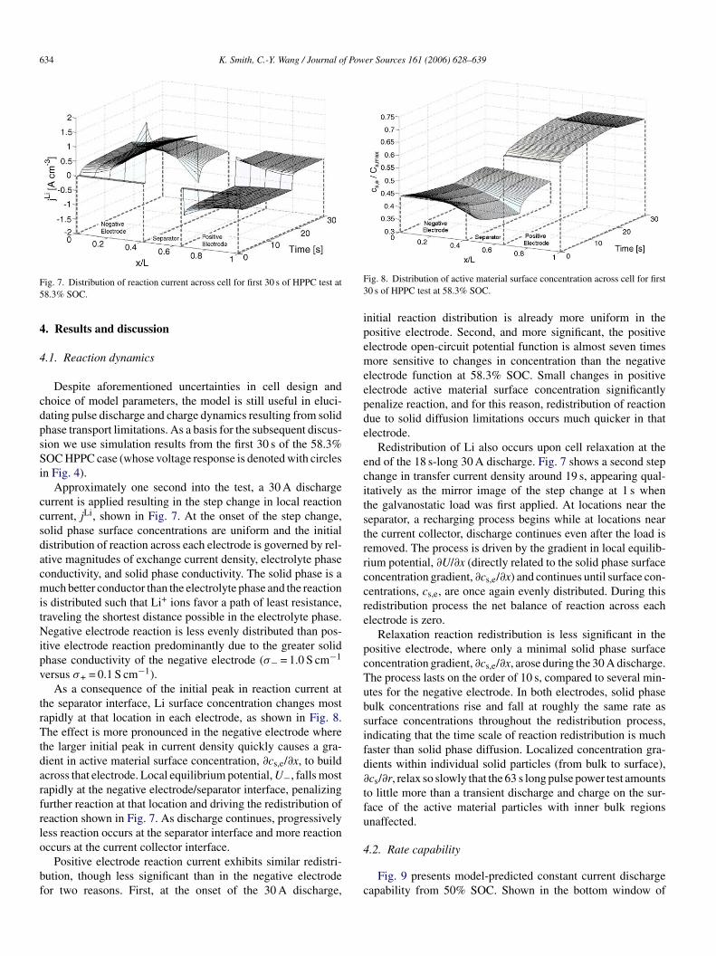
diation for 32 s, 22.5 A charge for 10 s, followed by open-circuitrelaxation as shown in the top window of Fig. 4. The onsetof constant current discharge and charge portions of the HPPCprofile are accompanied by brief (0.1 s) high-rate pulses to

K. Smith, C.-Y. Wang / Journal o

olid phase concentration at the particle surface, cs,e = cs|r=Rs ,o evaluate local equilibrium potential, U, and exchange currentensity, i0. Authors have used various approaches in their treat-ent of Eq. (4), including an analytical solution implemented asDuhamel superposition integral [11], a parabolic concentrationrofile model [19], and a sixth-order polynomial profile model20]. In the present work we approximate Eq. (4) using the finitelement method as described in Appendix A. Spatial discretiza-ion with five linear elements unevenly spaced along the particleadius provides sufficient resolution of cs,e(t) as a function ofLi(t) at both short and long times. The various approaches toolid-state diffusion modeling are contrasted and discussed inection 4.

For numerical solution, the 1D macroscopic domain isiscretized into approximately 70 control volumes in the x-irection. The solid diffusion submodel (Appendix A) is sep-rately applied within each control volume of the negative andositive electrodes. The four governing equations (Table 1) areolved simultaneously for field variables ce, cs,e, φe, and φs.urrent is used as the model input and boundary conditionsre therefore applied galvanostatically. Cell terminal voltage isetermined by the equation:

= φs|x=L − φs|x=0 − Rf

AI, (7)

here Rf represents a contact resistance between current collec-ors and electrodes.

. Model parameterization

Low-rate static discharge/charge, hybrid pulse power char-cterization (HPPC), and transient driving cycle data were pro-ided by the DOE FreedomCAR program for a 276 V nominalEV battery pack consisting of 72 serially connected cells. Dataas collected according to Freedom CAR test procedures [4].or the purpose of HEV systems integration modeling [21], weere tasked to build a mathematical model of single cell of thatack. We make no attempt to account for cell-to-cell variabilitynd present all data on a single cell basis by dividing measuredack voltage by 72. Due to the proprietary nature of the proto-ype FreedomCAR battery we were unable to disassemble cellso measure geometry, composition, etc., and thus adopt valuesrom the literature and adjust them as necessary to fit the data.y expressing capacity of the negative and positive electrodess

− = εs−(L−A)(cs,max−)(�x)F,

+ = εs+(L+A)(cs,max+)(�y)F, (8)

ow-rate capacity data provides a rough gauge of electrodeolume and stoichiometry cycling range, assuming electrodeomposition and electrode mass ratio values from Ref. [2]. Thisass ratio is later shown to result in a well-balanced cell at both

igh and low rates. Discharge capacity at the 1 C (6 A) rate waseasured to be 7.2 Ah and we define stoichiometry reference

oints for 0% and 100% SOC (listed in Table 2) on a 7.2 Ahasis.

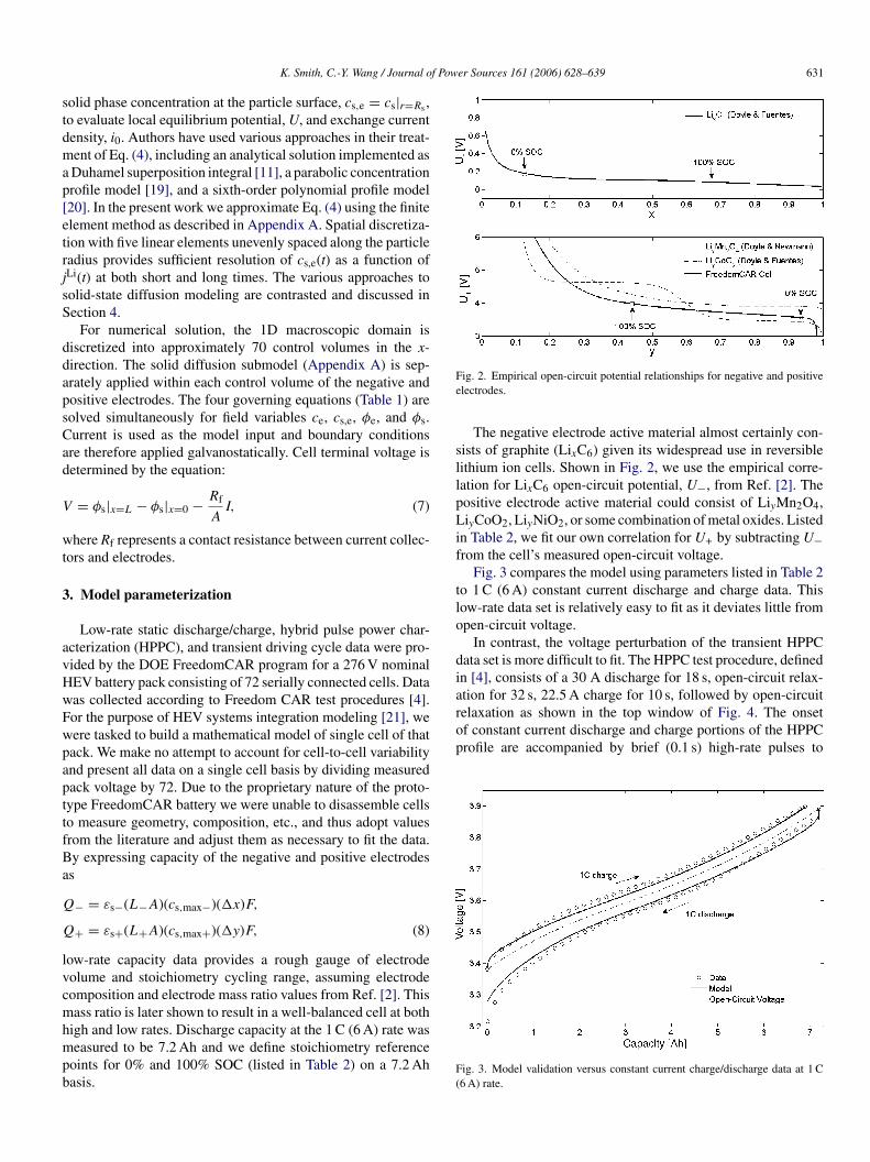
F(

ig. 2. Empirical open-circuit potential relationships for negative and positivelectrodes.

The negative electrode active material almost certainly con-ists of graphite (LixC6) given its widespread use in reversibleithium ion cells. Shown in Fig. 2, we use the empirical corre-ation for LixC6 open-circuit potential, U−, from Ref. [2]. Theositive electrode active material could consist of LiyMn2O4,iyCoO2, LiyNiO2, or some combination of metal oxides. Listed

n Table 2, we fit our own correlation for U+ by subtracting U−rom the cell’s measured open-circuit voltage.

Fig. 3 compares the model using parameters listed in Table 2o 1 C (6 A) constant current discharge and charge data. Thisow-rate data set is relatively easy to fit as it deviates little frompen-circuit voltage.

In contrast, the voltage perturbation of the transient HPPCata set is more difficult to fit. The HPPC test procedure, definedn [4], consists of a 30 A discharge for 18 s, open-circuit relax-

ig. 3. Model validation versus constant current charge/discharge data at 1 C6 A) rate.

632 K. Smith, C.-Y. Wang / Journal of Power Sources 161 (2006) 628–639

Table 2FreedomCAR cell model parameters

Parameter Negative electrode Separator Positive electrode

Design specifications (geometry and volume fractions)Thickness, δ (× 10−4 cm) 50 25.4 36.4Particle radius, Rs (× 10−4 cm) 1 1Active material volume fraction, εs 0.580 0.500Polymer phase volume fraction, εp 0.048 0.5 0.110Conductive filler volume fraction, εf 0.040 0.06Porosity (electrolyte phase volume fraction), εe 0.332 0.5 0.330

Solid and electrolyte phase Li+ concentrationMaximum solid phase concentration cs,max (× 10−3 mol cm−3) 16.1 23.9Stoichiometry at 0% SOC, x0%, y0% 0.126 0.936Stoichiometry at 100% SOC, x100%, y100% 0.676 0.442Average electrolyte concentration, ce (× 10−3 mol cm−3) 1.2 1.2 1.2

Kinetic and transport propertiesExchange current density, i0 (× 10−3 A cm−2) 3.6 2.6Charge-transfer coefficients, αa, αc 0.5, 0.5 0.5, 0.5SEI layer film resistance, RSEI (� cm2) 0 0Solid phase Li diffusion coefficient, Ds (× 10−12 cm2 s−1) 2.0 3.7Solid phase conductivity, σ (S cm−1) 1.0 0.1Electrolyte phase Li+ diffusion coefficient, De (× 10−6 cm2 s−1) 2.6 2.6 2.6Bruggeman porosity exponent, p 1.5 1.5 1.5Electrolyte phase ionic conductivity, κ (S cm−1) κ = 0.0158ce exp(0.85c1.4

e ) κ = 0.0158ce exp(0.85c1.4e ) κ = 0.0158ce exp(0.85c1.4

e )Electrolyte activity coefficient, f± 1.0 1.0 1.0Li+ transference number, t0+ 0.363 0.363 0.363

Parameter Value

Equilibrium potentialNegative electrode, U− (V) U−(x) = 8.00229 + 5.0647x− 12.578x1/2 − 8.6322 × 10−4x−1 + 2.1765 × 10−5x3/2 −

0.46016 exp[15.0(0.06 − x)] − 0.55364 exp[−2.4326(x− 0.92)]Positive electrode, U+ (V) U+(y) = 85.681y6 − 357.70y5 + 613.89y4 − 555.65y3 + 281.06y2 − 76.648y −

0.30987 exp(5.657y115.0) + 13.1983

Plate area-specific parametersElectrode plate area, A (cm2) 10452Current collector contact resistance, Rf (� cm2) 20

Fig. 4. Model validation versus HPPC test data. SOC labeled on 6 Ah-basisper FreedomCAR test procedures. SOC initial conditions used in 7.2 Ah-basismodel are 41.7%, 50.0%, 58.3%, 66.6%, and 75.0%.

eotp

ledwto[cfcpadau

n

stimate high-frequency resistance. Unable to decouple valuesf SEI layer resistance from contact film resistance (or cell-o-cell interconnect resistance for that matter), we fit ohmicerturbation using a contact film resistance of Rf = 20� cm2.

Neglecting double-layer capacitance for reasons noted ear-ier, the only transient phenomena accounted for in the gov-rning equations (here and in other work [14]) are electrolyteiffusion and solid diffusion. A parametric study showed thathile it was possible to match the observed voltage drop at

he end of the HPPC 30 A discharge by lowering De severalrders of magnitude from a baseline value of 2.6 × 10−6 cm2 s−1

2], the voltage drop at short times was too severe. Signifi-ant decrease in De also caused predicted voltage to divergerom the measured voltage over time due to severe electrolyteoncentration gradients. While recent LiPF6-based electrolyteroperty measurements [22] show diffusion coefficient, De, andctivity coefficient, f±, both exhibiting moderate concentrationependency, it is beyond the scope of this work to consider

nything beyond the first approximation of constant De andnity f±.

In investigating solid-state diffusion transient effects, weote that measured voltage response only allows observation

f Power Sources 161 (2006) 628–639 633

oDeip(gtlap

fmfistdsvtggfl

c

AwI

n

D

owutmdimtdtiSge(Httc

Fph

tt

sbcDmp

twas used to mimic a power profile recorded from a Toyota PriusHEV on a federal urban (FUDS) driving cycle. Only the first150 s are shown, though results are representative of the entiretest.

K. Smith, C.-Y. Wang / Journal o

f characteristic time t = R2s/Ds and will not provide Rs and

s independently. SEM images, such as that shown by Deest al. [23] (their Fig. 1) of a LiNi0.8Co0.15Al0.05O2 compos-te electrode, often show bulk or “secondary” active materialarticles (with radii ∼5 �m) having finer “primary” particleswith radii ∼0.5 �m) attached to the surface. Dees achievedood description of LiNi0.8Co0.15Al0.05O2 impedance data inhe 0.01–1 Hz frequency range using a characteristic diffusionength of 1.0 �m. As active material composition and structurere unknown for the present cell, we adopt this value as thearticle radius in both electrodes.

Though LixC6 is often reported to have more sluggish dif-usion than common positive electrode active materials, a para-etric study on Ds− using the transient solid diffusion model

ound no value capable of describing both the ∼0.047 V dropn cell voltage from 2 to 20 s of the HPPC test as well as thelow voltage relaxation upon open-circuit at 20 s. Assuming forhe moment that the ∼0.047 V drop is caused solely by solidiffusion limitations in the negative electrode, we estimate thaturface concentration cs,e− would need to fall from its initialalue by 4.3 × 10−4 mol cm−3 (a substantial amount) to causehe observed 0.047 V change in U−. Wang and Srinivasan [24]ive an empirical formula for the evolution of a concentrationradient within a spherical particle subjected to constant surfaceux as

s,e(t) − cs,avg(t) = jLi −Rs

5asFDs

[1 − exp

(−20

3

√Dst

Rs

)].

(9)

t steady state (where the exponential term goes to zero) andith the assumption of uniform reaction current density, jLi− =/AL−, we manipulate Eq. (9) to obtain a rough estimate of theegative electrode diffusion coefficient:

s− = Rs

5Fas�cs−I

AL−(10)

f 1.6 × 10−12 cm2 s−1. A corresponding characteristic timehereby the operand of the exponential term in Eq. (9) equalsnity is 140 s. Our conclusion is that, while a negative elec-rode solid diffusion coefficient of Ds− = 1.6 × 10−12 cm2 s−1

ight cause the cell voltage to drop ∼0.047 V, that voltagerop would take much longer to develop than what we observen the data. Repeating calculations for concentration gradient

agnitude and characteristic time under a variety of condi-ions revealed that the observed transient behavior might beescribed by solid-state diffusion in the negative electrode ifhe slope ∂U−/∂cs− were roughly eight times steeper. Thiss indeed the case in the positive electrode, where at 50%OC the open-circuit potential function has almost seven timesreater slope with respect to concentration than the negativelectrode. Chosen via parametric study, final values of Ds−2.0 × 10−12 cm2 s−1) and Ds+ (3.7 × 10−12 cm2 s−1) represent

PPC voltage dynamics in Fig. 4 quite well, although we note

hey are dependent upon our choice of particle radius. Were weo chose particle radii of 5 �m rather than 1 �m, our diffusionoefficient would be 25 times higher to maintain characteristic

Foc

ig. 5. Nominal model compared to models where limitations of electrolytehase, negative electrode solid phase, and positive electrode solid phase diffusionave been individually (not sequentially) removed.

ime t = R2s/Ds and match the voltage dynamics of the HPPC

est.Fig. 5 quantifies voltage polarization resulting from diffu-

ional transport by individually raising each diffusion coefficienty five or more orders of magnitude such that it no longer affectsell voltage response. Despite comparable values of Ds− ands+, the positive electrode polarizes transient voltage responseore significantly due to its stronger open-circuit potential cou-

ling.Fig. 6 compares model voltage prediction to data taken on

he FreedomCAR battery whereby an ABC-150 battery tester

ig. 6. Model validation versus transient FUDS cycle HEV data. Power profilef data mimics that recorded from a Toyota Prius (passenger car) HEV run on ahassis dynamometer.

634 K. Smith, C.-Y. Wang / Journal of Power Sources 161 (2006) 628–639

F5

4

4

cdpsSi

ccsdacmitNipv

trTtdarfrlo

bf

F3

ipemeepde

ecitstrrccre

pcTubsifd∂

tfu

ig. 7. Distribution of reaction current across cell for first 30 s of HPPC test at8.3% SOC.

. Results and discussion

.1. Reaction dynamics

Despite aforementioned uncertainties in cell design andhoice of model parameters, the model is still useful in eluci-ating pulse discharge and charge dynamics resulting from solidhase transport limitations. As a basis for the subsequent discus-ion we use simulation results from the first 30 s of the 58.3%OC HPPC case (whose voltage response is denoted with circles

n Fig. 4).Approximately one second into the test, a 30 A discharge

urrent is applied resulting in the step change in local reactionurrent, jLi, shown in Fig. 7. At the onset of the step change,olid phase surface concentrations are uniform and the initialistribution of reaction across each electrode is governed by rel-tive magnitudes of exchange current density, electrolyte phaseonductivity, and solid phase conductivity. The solid phase is auch better conductor than the electrolyte phase and the reaction

s distributed such that Li+ ions favor a path of least resistance,raveling the shortest distance possible in the electrolyte phase.egative electrode reaction is less evenly distributed than pos-

tive electrode reaction predominantly due to the greater solidhase conductivity of the negative electrode (σ− = 1.0 S cm−1

ersus σ+ = 0.1 S cm−1).As a consequence of the initial peak in reaction current at

he separator interface, Li surface concentration changes mostapidly at that location in each electrode, as shown in Fig. 8.he effect is more pronounced in the negative electrode where

he larger initial peak in current density quickly causes a gra-ient in active material surface concentration, ∂cs,e/∂x, to buildcross that electrode. Local equilibrium potential, U−, falls mostapidly at the negative electrode/separator interface, penalizingurther reaction at that location and driving the redistribution ofeaction shown in Fig. 7. As discharge continues, progressivelyess reaction occurs at the separator interface and more reaction

ccurs at the current collector interface.

Positive electrode reaction current exhibits similar redistri-ution, though less significant than in the negative electrodeor two reasons. First, at the onset of the 30 A discharge,

4

c

ig. 8. Distribution of active material surface concentration across cell for first0 s of HPPC test at 58.3% SOC.

nitial reaction distribution is already more uniform in theositive electrode. Second, and more significant, the positivelectrode open-circuit potential function is almost seven timesore sensitive to changes in concentration than the negative

lectrode function at 58.3% SOC. Small changes in positivelectrode active material surface concentration significantlyenalize reaction, and for this reason, redistribution of reactionue to solid diffusion limitations occurs much quicker in thatlectrode.

Redistribution of Li also occurs upon cell relaxation at thend of the 18 s-long 30 A discharge. Fig. 7 shows a second stephange in transfer current density around 19 s, appearing qual-tatively as the mirror image of the step change at 1 s whenhe galvanostatic load was first applied. At locations near theeparator, a recharging process begins while at locations nearhe current collector, discharge continues even after the load isemoved. The process is driven by the gradient in local equilib-ium potential, ∂U/∂x (directly related to the solid phase surfaceoncentration gradient, ∂cs,e/∂x) and continues until surface con-entrations, cs,e, are once again evenly distributed. During thisedistribution process the net balance of reaction across eachlectrode is zero.

Relaxation reaction redistribution is less significant in theositive electrode, where only a minimal solid phase surfaceoncentration gradient, ∂cs,e/∂x, arose during the 30 A discharge.he process lasts on the order of 10 s, compared to several min-tes for the negative electrode. In both electrodes, solid phaseulk concentrations rise and fall at roughly the same rate asurface concentrations throughout the redistribution process,ndicating that the time scale of reaction redistribution is muchaster than solid phase diffusion. Localized concentration gra-ients within individual solid particles (from bulk to surface),cs/∂r, relax so slowly that the 63 s long pulse power test amountso little more than a transient discharge and charge on the sur-ace of the active material particles with inner bulk regionsnaffected.

.2. Rate capability

Fig. 9 presents model-predicted constant current dischargeapability from 50% SOC. Shown in the bottom window of

K. Smith, C.-Y. Wang / Journal of Power Sources 161 (2006) 628–639 635

Ftf

FowiaEtacppxmt

fata5ttdgbbembiht

4

m

Fp

p

r

j

i

wt

T

c

wdmdrn

mcthe present model to cause end of discharge as the negative elec-trode nears depletion, is calculated by evaluating Eq. (14) atr = 1. Penetration depth, δ, providing a measure of active mate-

ig. 9. Solid phase surface concentration (top), minimum electrolyte concen-ration (middle), and time (bottom) at end of galvanostatic discharge for ratesrom 10 to 40 C.

ig. 9, a 40 C rate current (240 A) can be sustained for justver 6 s before voltage decays to the 2.7 V minimum. The topindow of Fig. 9 shows active material surface concentration

n the negative (left axis) and positive (right axis) electrodest the end of discharge across the range of discharge rates.lectrode-averaged rather than local values of surface concen-

ration are presented to simplify the discussion. The electrodesre fairly well balanced, indicated by end of discharge surfaceoncentrations near depletion and saturation in the negative andositive electrodes, respectively. End of discharge voltage isredominantly negative electrode-limited as stoichiometries of= cs,e/cs,max− < 0.05 causes a rapid rise in U−. Surface activeaterial utilization decreases slightly with increasing C-rate due

o increased ohmic voltage drop.In the present model, electrolyte Li+ transport is sufficiently

ast that electrolyte depletion does not play a limiting role atny discharge rate from 50% SOC. In the worst case of 30 C,he minimum value of local electrolyte concentration, occurringt the positive electrode/current collector interface, is around0% of average concentration, ce,0. For rates less than 30 C,he reduced current level results in lesser electrolyte concen-ration gradients, while for rates greater than 30 C, the shorteruration of discharge time results in a smaller concentrationradient at end of discharge. If we induce sluggish diffusiony reducing De (a similar effect may be induced in cell designy reducing porosity), electrolyte concentration in the positivelectrode comes closer to depletion with the worst case mini-um value of ce occurring at lesser current rates. Lowering De

y one order of magnitude for example, results in a battery lim-ted in the 10–20 C range by electrolyte phase transport, withigher and lower current rates still controlled by solid phaseransport.

.3. Solid-state diffusion limited current

Under solid phase transport limitations, simple relationshipsay be derived to predict maximum current available for a given

rfii

ig. 10. Dimensionless distribution of concentration within an active materialarticle at various times during galvanostatic (dis)charge.

ulse time. Substituting dimensionless variables:

= r

Rs, τ = Dst

R2s, cs(r, τ) = cs(r, τ) − cs,0

cs,max,

¯Li = jLiRs

DsasFcs,max(11)

nto Eq. (4) yields the dimensionless governing equation:

∂cs

∂τ= 1

r2

∂

∂r

(r2 ∂cs

∂r

)(12)

ith initial condition cs(r, τ = 0) = 0 ∀ r and boundary condi-ions:

∂cs

∂r

∣∣∣∣r=0

= 0,∂cs

∂r

∣∣∣∣r=1

= jLi. (13)

he solution given by Carslaw and Jaeger [25] is

¯s(r, τ)= − jLi

[3τ+ 1

10(5r2 − 3)−2

r

∞∑n=1

sin(λnr) exp(−λ2nτ)

λ2n sin(λn)

],

(14)

here the eigenvalues are roots of λn = tan(λn). Fig. 10 showsistribution of Li concentration along the radius of an activeaterial particle during galvanostatic discharge or charge for

imensionless times ranging from τ = 10−6 to 10−1 which, foreference, correspond to current pulses lasting 0.05–500 s usingegative electrode parameters from Table 2.

Surface concentration and depth of penetration into the activeaterial, both of practical interest for HEV pulse-type operation,

an be obtained from Eq. (14). Surface concentration, shown for

ial accessible for short duration pulse events, is calculated bynding the point along the radius where the concentration profile

s more or less equal to the initial condition. A 99% penetration

636 K. Smith, C.-Y. Wang / Journal of Pow

Table 3Empirical formulae fit to solid-state diffusion PDE exact solution, Eq. (14)

1% error bounds

Dimensionless surface concentrationcs,e

jLi= −1.139

√τ (16) 0 < τ < 1 × 10−4

cs,e

jLi= −1.122

√τ − 1.25τ (17) 0 < τ < 8 × 10−2

Dimensionless 99% penetration depthδ = 3.24

√τ (18) 0 < τ < 1 × 10−3√

dr

wlt

trfτ

tnTF

ttlacc

Fdf

s

vets

I

Wtssupbtid

4c

pfttj

δ = 3.23 τ + 1.89τ (19) 0 < τ < 2 × 10−2

epth, δ= Rs − r, is defined using the location r resulting in aoot of the formula:

cs(r, τ)

cs(1, τ)= 1 − a (15)

ith a = 0.99. Expressed as a fraction of total radius, dimension-ess penetration depth, δ = δ/Rs, is a function of dimensionlessime only.

Empirical expressions for dimensionless surface concentra-ion, cs,e, and dimensionless penetration depth, δ, are fit to theesults of Eq. (14) and presented in Table 3. Functions of theorm f (τ) = C

√τ provide good resolution at short times of

< 10−3, corresponding in our model to pulses lasting fewerhan ∼5 s. Resolution may be extended one to two orders of mag-itude in τ by using functions of the form f (τ) = C

√τ +Dτ.

he latter functions are plotted versus the exact solution (14) inig. 11.

Eq. (17) in Table 3 may be used in lieu of the present elec-rochemical model to predict negative electrode surface concen-rations for pulses shorter than 400 s, or, conversely, to predictimiting currents at rates greater than ∼9 C caused by depleted

ctive material surface concentration at end of discharge. Byombining Eqs. (11) and (17) under the assumption of uniformurrent density, jLi− = I/AL−, we obtain an empirical relation-

ig. 11. Dimensionless active material surface concentration and penetrationepth versus time (top). Percent error in empirical correlations of the form(τ) = C

√τ +Dτ (bottom).

c

Hcptprmfciiv

C

ω

I(

er Sources 161 (2006) 628–639

hip for surface concentration as a function of current and time:

cs,e(t)

cs,max−= cs,0

cs,max−− I

Rs−L−ADs−as−Fcs,max−

×[

1.122

√Ds−tRs−

+ 1.25Ds−tR2

s−

](20)

alid for t < 0.08Ds/R2s . Alternatively, given initial stoichiom-

try, x0, and surface stoichiometry at end of discharge, xs,e final,he maximum current available for a pulse discharge lasting teconds will be

max = (x0 − xs,e final)

⎛⎝L−Aas−Fcs,max−

1.122√Ds−

√t + 1.25

Rs− t

⎞⎠ . (21)

hile the theoretical maximum current will be obtained underhe condition xs,e final = 0, i.e. complete surface depletion, Fig. 9howed the present model to exhibit an end of discharge surfacetoichiometry around 0.03, with some rate dependency. Underniform initial conditions, the initial stoichiometry, x0, is sim-ly a function of SOC. For a recently charged or dischargedattery with nonuniform initial concentration, a better predic-ion of maximum pulse current may be obtained by replacing x0n Eq. (21) with a stoichiometry averaged across the penetrationepth or “pulse-accessible” region [26].

.4. Suitability of solid-state diffusion approximations forell modeling

Introduced in Section 2 and detailed in Appendix A, theresent work utilizes a fifth-order finite element approximationor solid-state diffusion (4) and incorporates that submodel intohe 1D electrochemical model as a finite difference equation,hat is, local values of cs,e are calculated using values of cs,e andLi from the previous five time steps:

[k]s,e = f ([c[k−1]

s,e , . . . , c[k−5]s,e ], [jLi[k], . . . , jLi[k−5]]). (22)

ere we compare the finite element submodel to the analyti-al solution employed by Doyle et al. [11] and the polynomialrofile model of Wang et al. [19]. Comparisons are made inhe frequency domain in order to remove the influence of aarticular type of input (pulse current, current step, constant cur-ent, etc.) by taking the Laplace transform of each time domainodel, expressing the input/output relationship as a transfer

unction in the Laplace variable s, and substituting s = jω toalculate the complex impedance at frequency ω. A capital-zed variable denotes that variable’s Laplace transform, thats, Cs,e(s) = L{cs,e(t)}, and an overbar denotes a dimensionlessariable. Define

¯ s,e(s) = Cs,e(s) − cs,0

cs,max, JLi(s) = JLi(s)

Rs

asFDscs,max,

2

¯ = ωRs

Ds. (23)

n the Laplace domain, a compact analytical solution to Eq.4) is readily available. The exact transfer function expressing

f Power Sources 161 (2006) 628–639 637

dt

w

tAs

a

Tcctqtfitτ

a

dacvawat

Fif

Ffi

tis

tatpsdnfm

K. Smith, C.-Y. Wang / Journal o

imensionless surface concentration versus dimensionless reac-ion current given by Jacobsen and West [28] is

Cs,e(s)

JLi(s)= tanh(ψ)

tanh(ψ) − ψ, (24)

here ψ = Rs√s/Ds.

Doyle et al. [11] provide two analytical series solutions inhe time domain, one for short times and one for long times. Inppendix B, we manipulate Doyle’s formulae to arrive at the

hort time transfer function:

Cs,e(s)

JLi(s)=

[1 − ψ + 2ψ

∞∑n=1

exp(−2nψ)

]−1

(25)

nd the long time transfer function:

Cs,e(s)

JLi(s)=

⎡⎣−2

∞∑n=1

ψ2

ψ2 + (nπRs)2

Ds

⎤⎦

−1

. (26)

he frequency response (magnitude and phase angle) of trun-ated versions of the short and long time transfer functions areompared to the exact transfer function (24) in Fig. 12, showinghe short time solution to provide good agreement at high fre-uencies and the long time solution at low frequencies. Note thathe short time transfer function does not change much beyond therst term of the series. A good strategy to piece together Doyle’s

wo solutions is to use one term of the short time solution for= Dst/R

2s ≤ 0.1 (corresponding to ω = 6 × 101 in Fig. 12)

nd around 100 terms of the long time solution for τ > 0.1.Reaction current appears in Eq. (4) as a time depen-

ent boundary condition which Doyle accommodates usingDuhamel superposition integral. Numerical solution of this

onvolution-type integral requires that a time history of all pre-ious step changes in surface concentration be held in memory

nd called upon at each time step to reevaluate the integral. Sohile the analytical solution is inarguably the most accurate

pproach, it can be expensive in terms of memory and computa-ional requirements, particularly in situations requiring a small

ig. 12. Frequency response of short and long time analytical solutions usedn Ref. [11] for solid-state diffusion in spherical particles, compared to exactrequency response from Ref. [28].

SpopRr3sem

sdtm

Fo

ig. 13. Frequency response of parabolic profile solid-state diffusion submodelrom Ref. [19] and fifth-order finite element solid-state diffusion submodel (usedn this work), compared to exact frequency response from Ref. [28].

ime step but long simulation time (driving cycle simulations, fornstance) or in situations requiring a large grid mesh (2D or 3Dimulations incorporating realistic cell geometry, for instance).

Approximate solutions to Eq. (4) are appropriate so long ashey capture solid-state diffusion dynamics sufficiently fast forparticular investigation. Wang et al. [19] assume the concen-

ration profile within the spherical particle is described by aarabolic profile cs(r, t) = A(t) + B(t)r2, and thus formulate aolid-state diffusion submodel which correctly captures bulkynamics and steady state concentration gradient, but otherwiseeglects diffusion dynamics. Derived in Appendix C, the trans-er function of the parabolic profile, or steady state diffusion,odel is

Cs,e(s)

JLi(s)= 3

ψ2 + 1

5. (27)

hown in Fig. 13 versus the exact transfer function (24), thearabolic profile model is valid for low frequencies, ω < 10,r long times, τ = Dst/R

2s > 0.6. Substituting values from the

resent model’s negative electrode (Ds− = 2.0 × 10−12 cm2 s−1,s− = 1.0 × 10−4 cm), the parabolic profile model would cor-

ectly predict surface concentration only at times longer than000 s. For electrochemical cells with sluggish solid-state diffu-ion, the parabolic profile model will correctly capture low-ratend of discharge behavior, but is generally inappropriate in theodeling of high rate (>2 C) or pulse type applications [27].We find spatial discretization of Eq. (4) yields low-order

olid-state diffusion models with more accurate short time pre-iction compared to polynomial profile models [20]. Recastinghe fifth-order finite element model from Appendix A in nondi-

ensional form:

Cs,e(s)

JLi(s)= asF

Ds

Rs

[b1s

5 + b2s4 + b3s

3 + b4s2 + b5s+ b6

a1s5 + a2s4 + a3s3 + a4s2 + a5s+ a6

].

(28)

ig. 13 shows the present model to provide good approximationf the exact transfer function (26) for ω < 105, and thus be valid

6 f Pow

fmncbs

5

dchdpctca

pLehedtwoc

A

OAWfD

A

A

pacmar

ccepb

s⎡⎢⎢⎢⎢⎣

wu1c

a

w(tsdu

G

r

wtmb

A

Bd

editf

a

T

a(τ) = −τ + 2τ

1 + 2 exp −n

38 K. Smith, C.-Y. Wang / Journal o

or dimensionless times τ > 6 × 10−5 (or t > 0.3 s for the presentodel’s negative electrode). Regardless of what solution tech-

ique is employed for solid-state diffusion in an electrochemicalell model, if the objective is to match high-rate (∼40 C) pulseehavior and predict transport limitations on a short (∼5 s) timecale, that technique must be valid at very short times.

. Conclusions

A fifth-order finite element model for transient solid-stateiffusion is incorporated into a previously developed 1D electro-hemical model and used to describe low-rate constant current,ybrid pulse power characterization, and transient driving cycleata sets from a lithium ion HEV battery. HEV battery models inarticular must accurately resolve active material surface con-entration at very short dimensionless times. Requirements forhe present model are t = Dst/R

2s ≈ 10−3 to predict 40 C rate

apability and τ≈ 2 × 10−5 to match current/voltage dynamicst 10 Hz.

Dependent on cell design and operating condition, end ofulse discharge may be caused by negative electrode solid phasei depletion, positive electrode solid phase Li saturation, orlectrolyte phase Li depletion. Simple expressions developedere for solid-state diffusion-limited current, applicable in eitherlectrode, may aid in the interpretation of high-rate experimentalata. While the present work helps to extend existing litera-ure into the dynamic operating regime of HEV batteries, futureork remains to fully characterize an HEV battery in the lab-ratory and develop a fundamental model capable of matchingurrent/voltage data at very high rates.

cknowledgements

This work was funded by the U.S. Department of Energy,ffice of FreedomCAR and Vehicle Technologies throughrgonne National Laboratory (Program Manager: Lee Slezak).e thank Aymeric Rousseau and Argonne National Laboratory

or providing battery experimental data as well as Dr. Marcoyle and Dr. Venkat Srinivasan for helpful discussions.

ppendix A

.1. Solid-state diffusion finite element model

The transient phenomenon of solid-state Li diffusion is incor-orated into the previously developed macroscopic model of Gund Wang [3]. While the governing Eq. (4) describes solid phaseoncentration along the radius of each spherical particle of activeaterial, the macroscopic model requires only the concentration

t the surface, cs,e(t), as a function of the time history of localeaction current density, jLi(t).

We transform the PDE, Eq. (4), from spherical to planaroordinates using the substitution v(r) = rcs(r) [28,29] and dis-

retize the transformed equation in the r-direction with n linearlements. (The present model uses five elements with nodeoints placed at {0.7,0.91,0.97,0.99,1.0}× Rs.) Transformedack to spherical coordinates, the discretized system is repre-

er Sources 161 (2006) 628–639

ented as ODEs in state space form:

cs,1

cs,2

...

cs,n

⎤⎥⎥⎥⎥⎦ = A

⎡⎢⎢⎢⎢⎣cs,1

cs,2

...

cs,n

⎤⎥⎥⎥⎥⎦ + BjLi, cs,e ≈ C

⎡⎢⎢⎢⎢⎣cs,1

cs,2

...

cs,n

⎤⎥⎥⎥⎥⎦ + DjLi,

(A.1)

here the n states of the system are the radially distributed val-es of concentration cs,1, . . ., cs,n, at finite element node points, . . ., n. For the linear PDE (4) with constant diffusion coeffi-ient, Ds, the matrix A is constant and tri-diagonal.

The linear state space system (A.1) can also be expressed astransfer function:

cs,e(s)

jLi(s)≈ G(s) = b1s

n + b2sn−1 + · · · + bn−1s+ bn

a1sn + a2sn−1 + · · · + an−1s+ an(A.2)

ith constant coefficients ai and bi [30]. While either (A.1) orA.2) could be numerically implemented using an iterative solu-ion method, we exploit the linear structure of (4) and express theystem as a finite difference equation with explicit solution. Toiscretize (A.2) with respect to time, we perform a z-transformsing Tustin’s method:

T(z) = G(s)|s=(2/Ts)((z−1)/(z+1)), (A.3)

esulting in an nth-order discrete transfer function:

cs,e(z)

jLi(z)≈ GT(z) = h1z

n + h2zn−1 + · · · + hn−1z+ hn

g1zn + g2zn−1 + · · · + gn−1z+ gn(A.4)

ith constant coefficients hi and gi. Computation is thus reducedo an explicit algebraic formula with minimal memory require-

ents. Solution for cs,e requires that local values of cs,e and jLi

e held from only the previous n − 1 time steps.

ppendix B

.1. Transfer functions of short and long time solid-stateiffusion analytical solutions

Doyle et al. [11] employ an analytical solution to Eq. (4) andmbed it inside a Duhamel superposition integral to accommo-ate the time dependent boundary condition. They provide twontegral expressions for the response of reaction current, jLi(τ),o a step in surface concentration, �cs,e, at τ = 0, each in theorm

(τ) = 1

asF

Rs

Ds

1

�cs,e

∫ τ

0jLi(ζ) dζ. (B.1)

he short time expression (Eq. (B.6) of [11]) is√ [ ∞∑ ( 2 )

π

n=1τ

−n√π

τerfc

(n√τ

)], (B.2)

f Pow

w

a

Lfj

j

a

j

n(i

a

Td(

A

Cd

sptct

a

c

T

s

a

C

wf

S(

R

[

[

[

[[

[[[

[

[[

[[

[

[[

[

[

[[29] M.N. Ozisik, Heat Conduction, John Wiley & Sons, New York, 1993, pp.

K. Smith, C.-Y. Wang / Journal o

hile the long time expression (Eq. (B.5) of [11]) is

(τ) = 2

π2

∞∑n=1

1

n2 [1 − exp(−n2π2τ)]. (B.3)

ittle detail is given in the derivation of these expressions. Dif-erentiating Eqs. (B.1)–(B.3) with respect to τ and solving forLi(τ), we recover short time solution:

Li(τ) = asFDs

Rs

[1 − 1√

πτ+ 2√

πτ

∞∑n=1

exp

(−n

2

τ

)]�cs,e

(B.4)

nd long time solution:

Li(τ) = asFDs

Rs

[−2

∞∑n=1

exp(−n2π2τ)

]�cs,e (B.5)

o longer in integral form. Taking the Laplace transform of Eqs.B.4) and (B.5) and recognizing that the transform of the stepnput is Cs,e(s) =�cs,e/s, we find the short time transfer function:

JLi(s)

Cs,e(s)= asF

Ds

Rs

[1 − Rs

√s

Ds+ 2Rs

√s

Ds

∞∑n=1

×exp

(−2nRs

√s

Ds

)](B.6)

nd the long time transfer function:

JLi(s)

Cs,e(s)= asF

Ds

Rs

[−2

∞∑n=1

s

s+ n2π2

]. (B.7)

aking the reciprocal of Eqs. (B.6) and (B.7) and substitutingimensionless variables JLi, Cs,e, and ψ yields Eqs. (25) and26) respectively, used in Section 4.4.

ppendix C

.1. Transfer function of parabolic profile solid-stateiffusion approximate model

Wang et al. [19] assume concentration distribution within apherical active material particle to be described by a parabolicrofile. Integrating the two parameter polynomial with respecto Eq. (4), they reduce the problem of determining surface con-entration, cs,e(t), as a function of reaction current, jLi(t), downo the solution of one ODE:

∂cs,avg

∂t= 3

asFRsjLi (C.1)

nd one interfacial balance:

s,e − cs,avg = Rs

5asFDsjLi. (C.2)

aking the Laplace transform of Eqs. (C.1) and (C.2) yields:

Cs,avg(s) = 3

asFRsJLi(s) (C.3)

[

er Sources 161 (2006) 628–639 639

nd

s,e(s) − Cs,avg(s) = Rs

5asFDsJLi(s), (C.4)

hich when combined to eliminate Cs,avg, provides the transferunction:Cs,e(s)

JLi(s)= 1

asF

Rs

Ds

[3Ds

sR2s

+ 1

5

]. (C.5)

ubstituting dimensionless variables JLi, Cs,e, and ψ into Eq.C.5) yields Eq. (27), used in Section 4.4.

eferences

[1] M. Doyle, J. Newman, A.S. Gozdz, C.N. Schmutz, J.M. Tarascon, J. Elec-trochem. Soc. 143 (1996) 1890–1903.

[2] M. Doyle, Y. Fuentes, J. Electrochem. Soc. 150 (2003) A706–A713.[3] W.B. Gu, C.Y. Wang, ECS Proc. 99-25 (2000) 748–762.[4] FreedomCAR Battery Test Manual For Power-Assist Hybrid Electric Vehi-

cles, DOE/ID-11069, 2003.[5] P. Nelson, I. Bloom, K. Amine, G. Hendriksen, J. Power Sources 110 (2002)

437–444.[6] S. Al Hallaj, H. Maleki, J. Hong, J. Selman, J. Power Sources 83 (1999)

1–8.[7] P. Nelson, D. Dees, K. Amine, G. Henriksen, J. Power Sources 110 (2002)

349–356.[8] E. Karden, S. Buller, R. DeDoncker, Electrochem. Acta 47 (2002)

2347–2356.[9] S. Barsali, M. Ceraolo, Electrochem. Acta 47 (2002) 2347–2356.10] J. Christophersen, D. Glenn, C. Motloch, R. Wright, C. Ho, Proceedings of

the IEEE Vehicular Technology Conference, vol. 56, Vancouver, Canada,2002, pp. 1851–1855.

11] M. Doyle, T. Fuller, J. Newman, J. Electrochem. Soc. 140 (1993)1526–1533.

12] M. Doyle, T. Fuller, J. Newman, Electrochem. Acta 39 (1994) 2073–2081.

13] T. Fuller, M. Doyle, J. Newman, J. Electrochem. Soc. 141 (1994) 1–10.14] T. Fuller, M. Doyle, J. Newman, J. Electrochem. Soc. 141 (1994) 982–

990.15] I. Ong, J. Newman, J. Electrochem. Soc. 146 (1999) 4360–4365.16] M. Doyle, J. Meyers, J. Newman, J. Electrochem. Soc. 147 (2000) 99–110.17] J. Meyers, M. Doyle, R. Darling, J. Newman, J. Electrochem. Soc. 147

(2000) 2930–2940.18] P. Arora, M. Doyle, R. White, J. Electrochem. Soc. 146 (1999) 3543–

3553.19] C.Y. Wang, W.B. Gu, B.Y. Liaw, J. Electrochem. Soc. 145 (1998) 3407.20] V. Subramanian, J. Ritter, R. White, J. Electrochem. Soc. 148 (2001)

E444–E449.21] K. Smith, C.Y. Wang, J. Power Sources 160 (2006) 662–673.22] L.O. Valøen, J.N. Reimers, J. Electrochem. Soc. 152 (2005) A882–

A891.23] D. Dees, E. Gunen, D. Abraham, A. Jansen, J. Prakash, J. Electrochem.

Soc. 152 (2005) A1409–A1417.24] C.Y. Wang, V. Srinivasan, J. Power Sources 110 (2002) 364–376.25] H.S. Carslaw, J.C. Jaeger, Conduction of Heat in Solids, Oxford University

Press, London, 1973, p. 112.26] K. Smith, C.Y. Wang, Proceedings of the SAE Future Transportation Tech-

nology Conference, Chicago, IL, September 7–9, 2005.27] G. Sikha, R.E. White, B.N. Popov, J. Electrochem. Soc. 152 (2005)

A1682–A1693.28] T. Jacobsen, K. West, Electrochem. Acta 40 (1995) 255–262.

327–334.30] G. Franklin, J.D. Powell, M. Workman, Digital Control of Dynamic

Systems, 3rd ed., Addison-Wesley/Longman, Menlo Park, CA,1998.