solitons in fiber optics

8/4/2019 Solitons in Fiber Optics

http://slidepdf.com/reader/full/solitons-in-fiber-optics 1/22

Solitons in optical communications

Hermann A. Haus and William S. Wong

Department of Electrical Engineering and Computer Science

and Research Laboratory of Electronics, Massachusetts Institute of Technology,

Cambridge, Massachusetts 02139

The history of the proposal that solitons be used for optical fiber communications and of the technical

developments toward making soliton transmission practical is reviewed. The causes of bit errors in

long-distance soliton transmission are presented and the methods for reducing them are described. Aperturbation theory suited for soliton analysis is developed. Current status and future prospects of

long-distance repeaterless fiber communications are stated.

CONTENTS

I. Introduction 423

II. The Nonlinear Schro ¨ dinger Equation 426

III. Properties of Solitons 428

IV. Perturbation Theory of Solitons 429

V. Amplifier Noise and the Gordon-Haus Effect 431

VI. Control Filters 432VII. Stimulated Raman Scattering and the Raman

Self-Frequency Shift 434

VIII. Continuum Generation 435

IX. Erbium-Doped Fiber Amplifiers and the Effect of

Lumped Gain 435

X. Polarization 437

XI. Discussion 438

Acknowledgments 439

Appendix A: Soliton Collision Effects 439

Appendix B: The Amplified Spontaneous Emission Noise Source 439

References 440

I. INTRODUCTION

The soliton concept is a sophisticated mathematicalconstruct based on the integrability of a class of nonlin-ear differential equations. Integrable nonlinear differen-tial equations have one feature in common: they are allconservative and are thus derivable from a Hamiltonian.The integration is performed via the method of inversescattering (Gardner et al., 1967).

The nonlinear Schro ¨ dinger equation is one member of the class of integrable equations. In their classic paper,Zakharov and Shabat (1971) presented the mathemati-cal framework, based on inverse scattering theory, forthe integration of the nonlinear Schro ¨ dinger equation.

Soon afterwards, Hasegawa and Tappert (1973) pointedout that solitons could be propagated on glass fibers withnegative (anomalous) group velocity dispersion (GVD)under the influence of the optical Kerr effect, in whichthere is a change of refractive index induced by the op-tical field. The GVD in glass fibers with a Ge-doped coreis controlled mainly by material dispersion, but it can beinfluenced somewhat by the index (doping) profile. Forwavelengths longer than 1.3 m, standard glass fibershave negative GVD.

Mollenauer, Stolen, and Gordon (1980) demonstratedthe propagation of solitons in optical fibers. Extensive

experiments were conducted by the group at Bell Labo-ratories; these confirmed the predictions of the nonlin-ear Schro ¨ dinger equation and proved that the propertiesof fiber propagation are described, to a remarkable de-gree, by this equation.

Hasegawa (1984) made the imaginative proposal thatsolitons could be used for ‘‘repeaterless’’ communica-tions over transoceanic distances. Conventional commu-nications using optical fibers at that time (and even to-day) detect, regenerate electronically, and retransmitoptically the bit-stream at every repeater. The repeaterdistances [120–150 km (Li, 1993)] are chosen to be aslarge as possible, while still permitting detection and re-generation of the signal with a net bit-error rate of lessthan 109. The ‘‘repeaterless’’ transmission concept pro-posed by Hasegawa would compensate the fiber losswith Raman gain.

One of the authors (H.A.H.) was spending part of asabbatical in 1984 at Bell Laboratories (renamed AT&TBell Laboratories after the breakup of AT&T). Learn-ing about the proposal, he and Gordon investigated pos-sible mechanisms that may get in the way of repeaterlesscommunications with solitons. The amplifiers needed tocompensate for the loss generate amplified spontaneousemission, and this noise is expected to degrade the soli-ton signal. This degradation is twofold in nature. Thesimple effect is that additive noise is generated at eachamplifier, which can be combatted by raising the signallevel. The more subtle effect is nonlinear, and was ana-lyzed by Gordon and Haus (1986): the noise is, in part,incorporated by the soliton, whose mean frequency isthen shifted. A frequency shift leads to a timing shiftbecause pulses of different frequencies have different

group velocities due to GVD. This timing shift is asource of errors. It was shown that this mechanismwould limit the distance of propagation to a still surpris-ingly large value of 2800 km for the parameters chosenby Hasegawa. After this limit was established, it wassoon shown by Mollenauer (Mollenauer and Smith,1988) that choice of a dispersion lower than that as-sumed by Hasegawa could extend the propagation dis-tance to transatlantic distances.

Mollenauer carried out pioneering experiments onlong distance optical communications using solitons(Mollenauer and Smith, 1988). He developed the fiber

423Reviews of Modern Physics, Vol. 68, No. 2, April 1996 0034-6861/96/68(2)/423(22)/$13.30 © 1996 The American Physical Society



loop system into which a bit stream is loaded and recir-culated, thereby simulating propagation over arbitrarilylarge distances using a few hundred kilometers of fiber.Initially he used Raman gain for loss compensation.Meanwhile, however, an erbium-doped fiber amplifierthat can be pumped by laser diodes was developed byDesurvire and others (Desurvire et al., 1987; Mearset al., 1987; Laming et al., 1989; Inoue et al., 1989, 1991;

Desurvire, Zyskind, and Giles, 1990; Desurvire, Zys-kind, and Simpson, 1990; Zyskind et al., 1990; Tachibanaet al., 1991). This fiber amplifier is a few meters long andhas remarkable properties (to be discussed in greaterdetail later). M. Nakazawa at Nippon Telegraph andTelephone Company (NTT) recognized their potentialfor soliton transmission and demonstrated their use inhis fiber loop experiments (Nakazawa et al., 1989; Naka-zawa, Suzuki, and Kimura, 1990).

It should be mentioned that the replacement of thedistributed Raman gain with ‘‘lumped’’ amplifiers wasan important advance. The soliton concept is associatedwith a lossless uniform fiber and hence one would expect

that the actual loss of the fiber would have to be com-pensated by distributed gain. This was the reason for theuse of Raman gain in which the pumped fiber itself acted as the gain medium. However, a more detailedinvestigation, which will be outlined further on, showsthat lumped gain is permissible provided that the ampli-fier spacing is not excessive. Mollenauer used 25 km am-plifier spacings in his experiments. However, spacings of 33 km, 50 km, and as large as 105 km have also beenused by other laboratories (see Table I).

In fiber loop experiments with erbium-doped amplifi-ers, Mollenauer and his group continued their experi-ments on long-distance propagation of solitons. The pre-diction by Gordon and Haus of the amplifiedspontaneous emission-induced bit errors was confirmedexperimentally (Mollenauer and Smith, 1988; Mol-lenauer, Neubelt et al., 1990; Mollenauer, Nyman et al.,1991). The effect being a nonlinear one, it limits thepeak pulse power permissible for transmission. The lin-ear additive noise establishes a lower limit on the peakpower. The range of powers permissible for transmissionat an acceptable bit-error rate (109) turned out to benarrow—too narrow for the system designers, if allow-ance was to be made for the aging of the amplifiers.

As happens so often, the long-distance soliton com-munications experiments spurred on the competition. If it is possible to send solitons, which compensate the

GVD with fiber nonlinearity, without repeaters overlong distances, why not send low-level signals ‘‘linearly’’over long distances on fibers that have zero GVD? Thisapproach has been taken at the AT&T Bell Laborato-ries (Runge, 1992; Bergano and Davidson, 1995; Forgh-ieri et al., 1995; Hansen et al., 1995; Kerfoot and Runge,1995), Kokusai Denshin Denwa Company, Ltd. (KDD)(Otani et al., 1995; Taga et al., 1995), Nippon Telegraphand Telephone Company (Kataoka et al., 1994; Mu-rakami et al., 1995), Hitachi (Kikuchi et al., 1995),Northern Telecom (Butler et al., 1994), Alcatel (Clescaet al., 1994; Gautheron et al., 1995), and British Telecom

(Gu et al., 1994). The transmission format is nonreturnto zero (NRZ). The signal is composed of roughly rect-angular pulses that merge into one block when two ormore occur consecutively. ‘‘Linear’’ transmission has toovercome serious obstacles of its own. Over the largetransoceanic distances with signal levels large enough todominate over the amplified spontaneous emission, it isimpossible to avoid the Kerr nonlinearity, which can

lead to serious signal distortion. The effect can begreatly reduced if the fiber is composed of segments withalternating positive and negative GVD; this tends toscramble the phase induced by the nonlinearity. Cablesusing fiber segments of alternating GVD have alreadybeen laid, and are operating at 5 Gbit/s between the U.S.and Europe, and between California and Hawaii. Sincethis paper is on soliton transmission, we shall not dwellfurther on this subject. One should note, however, thatthe eventual implementation of soliton communicationscan only occur if the soliton system delivers, at compa-rable cost, better performance than the existing and stilldeveloping NRZ systems.

Returning to the soliton story, which we left at around1990, we note that three major advances occurred in1991:

(a) Nakazawa and his group propagated solitons over106 km in a fiber loop containing, in addition to theerbium-doped amplifiers, amplitude modulators (Naka-zawa, Yamada et al., 1991). The amplitude modulatorsrestored the timing of solitons that had strayed from thecenter of the bit interval. This work showed that themodulators control the noise-induced timing jitter of thesolitons. It also raised the possibility that such loops canmaintain a bit stream of ‘‘ones’’ and ‘‘zeros’’ forever. Ina theoretical paper it was shown soon afterwards that acombination of modulators and filters is indeed capableof maintaining the ‘‘ones’’ in their assigned time slotsand in preventing the amplified spontaneous emissionnoise from building up in the ‘‘zero’’ slots, thus provid-ing signal storage (Haus and Mecozzi, 1992). The stor-age capability of fiber rings has been demonstrated sincethen (Doerr et al., 1994; Hall et al., 1995; Moores et al.,1995).

(b) In a closed-loop experiment, the amplitude modu-lator timing is derived from a common clock. In ‘‘open-loop’’ transoceanic transmission, the timing of themodulators must be derived from a local clock recovery,thus complicating the system. Furthermore, if the fibercarries wavelength-division multiplexed bit streams, the

timing of each of the channels differs due to GVD. Thusthe channels must be demultiplexed, the clock recoveredfrom each channel, each channel modulated separately,and finally the channels must be remultiplexed. This is acomplicated procedure that invites simpler alternatives.The discovery of a simpler means was made indepen-dently at MIT (Mecozzi et al., 1991), and by Kodamaand Hasegawa (1992) at AT&T Bell Laboratories. Theerbium-doped amplifiers have a gain bandwidth of theorder of 40 nm, while the solitons used in 5 Gbit/s trans-mission have a bandwidth of the order of 0.05 nm. Thefilters tend to keep the solitons at the center frequency

424 H. A. Haus and W. S. Wong: Solitons in optical communications

Rev. Mod. Phys., Vol. 68, No. 2, April 1996



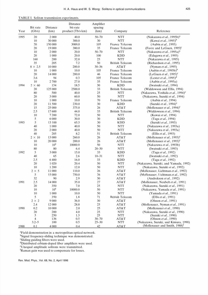
TABLE I. Soliton transmission experiments.

YearBit rate(Gb/s)

Distance(km)

Distancebit-rate

product (Tb/s km)

Amplifierspacing

(km) Company Reference

1995 20 2 000 40.0 50–70 NTT (Nakazawa et al., 1995b)a

10 30 000 300.0 30 NTT (Kawai et al., 1995)b

20 150 000 3000.0 105 France Telecom (Aubin et al., 1995)20 19 000 380.0 35 France Telecom (Favre and LeGuen, 1995)c

10 2 000 20.0 50–70 NTT (Nakazawa et al., 1995a)a

20 1 000 20.0 100 KDD (Edagawa et al., 1995)160 200 32.0 25 NTT (Nakazawa et al., 1995)35 205 7.2 50 British Telecom (Richardson et al., 1995)

8 2.5 10 000 200.0 30–36 AT&T (Nyman et al., 1995)10 1 000 10.0 105 France Telecom (Aubin et al., 1995b)b

20 14 000 280.0 46 France Telecom (LeGuen et al., 1995)c

3.6 94 0.3 105 France Telecom (Lester et al., 1995)d

10 2 700 27.0 35 France Telecom (Aubin et al., 1995a)1994 2 60 154 18.5 30 KDD (Iwatsuki et al., 1994)

20 125 000 2500.0 33 British Telecom (Widdowson and Ellis, 1994)80 500 40.0 25 NTT (Nakazawa, Yoshida et al., 1994)e

20 3 000 60.0 50 NTT (Nakazawa, Suzuki et al., 1994)10 1 000 10.0 70 France Telecom (Aubin et al., 1994)

20 11 500 230.0 30 KDD (Suzuki et al., 1994)e

15 25 000 375.0 26 AT&T (Mollenauer et al., 1994)c

2.5 17 600 44.0 33 British Telecom (Widdowson et al., 1994)10 7 200 72.0 50 NTT (Kawai et al., 1994)5 6 000 30.0 30 KDD (Taga et al., 1994)

1993 5 13 100 65.5 30 KDD (Suzuki et al., 1993)40 1 000 40.0 50 NTT (Nakazawa et al., 1993a)20 2 000 40.0 50 NTT (Nakazawa et al., 1993a)40 205 8.2 51 British Telecom (Ellis et al., 1993)

2 10 13 000 260.0 26 AT&T (Mollenauer et al., 1993)c

10 20 000 200.0 26 AT&T (Mollenauer et al., 1993)c

10 106 10000.0 50 NTT (Nakazawa et al., 1993b)80 80 6.4 20–30 NTT (Iwatsuki et al., 1993)

1992 5 3 000 15.0 33 KDD (Taga et al., 1992)

40 65 2.6 10–31 NTT (Iwatsuki et al., 1992)2.5 6 400 16.0 33 KDD (Taga et al., 1992)20 1 020 20.4 50 NTT (Nakazawa, Suzuki, and Yamada, 1992)10 1 200 12.0 50 NTT (Nakazawa, Suzuki et al., 1992)

2 5 11 000 110.0 26 AT&T (Mollenauer, Lichtman et al., 1992)5 15 000 750.0 26 AT&T (Mollenauer, Lichtman et al., 1992)

32 90 2.9 30 AT&T (Andrekson et al., 1992)1991 2.5 14 000 35.0 27 AT&T (Mollenauer, Neubelt et al., 1991)

20 350 7.0 25 NTT (Nakazawa, Suzuki et al., 1991)10 106 10000.0 50 NTT (Nakazawa, Yamada et al., 1991)10 1 000 10.0 50 NTT (Yamada et al., 1991)5 350 1.8 71 British Telecom (Ellis et al., 1991)

2 2 9 000 36.0 30 AT&T (Olsson et al., 1991)2.4 12 000 28.8 25 AT&T (Mollenauer, Nyman et al., 1991)

1990 0.2 10 000 2.0 25 AT&T (Mollenauer et al., 1990)20 200 4.0 25 NTT (Nakazawa, Suzuki et al., 1990)5 250 1.3 25 NTT (Suzuki et al., 1990)4 136 0.5 30–70 AT&T (Olsson et al., 1990)

3.2–5 100 0.5 25–30 NTT (Nakazawa, Suzuki, and Kimura, 1990)

1988 0.1 4 000 0.4 42 AT&T (Mollenauer and Smith, 1988)f

aField demonstration in a metropolitan optical network.bSignal frequency-sliding technique was demonstrated.cSliding guiding filters were used.dDistributed erbium-doped fiber amplifiers were used.eUnequal amplitude solitons were transmitted.f Raman gain was used to compensate for losses.

425H. A. Haus and W. S. Wong: Solitons in optical communications




of the filter, thus reducing the timing jitter. The twogroups proposed that filters be introduced at each am-plifier stage, having roughly ten times the signal band-width. The filters could be of the Fabry-Perot type thatcan accommodate wavelength-division multiplexedtransmission. This discovery widened the range of ac-ceptable peak pulse powers. The transmission distancewas still limited by the growth of narrow-band noise atthe center frequency (wavelength) of the filters, whichexperiences less loss than the filtered solitons.

(c) Based on this discovery, Mollenauer and cowork-ers developed the sliding guiding filter concept (Mol-lenauer, Gordon, et al., 1992; Mollenauer et al., 1993). Inthis scheme, the center frequency of the filters is dis-placed from amplifier to amplifier. The soliton carrierfrequency follows the filter center frequencies; narrow-band noise, on the other hand, sees filter loss on theaverage along the total length of transmission.

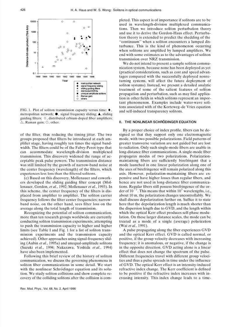
Recognizing the potential of soliton communication,more than ten research groups worldwide are currentlyconducting soliton transmission experiments, attemptingto push the transmission capacity to higher and higher

limits (see Table I and Fig. 1 for a list of soliton trans-mission experiments and the transmission capacityachieved). Other approaches using signal-frequency slid-ing (Aubin et al., 1995a) and unequal-amplitude solitons(Suzuki et al., 1994; Nakazawa, Yoshida et al., 1994)have also been implemented.

Following this brief review of the history of solitoncommunication, we discuss the governing phenomena insoliton fiber communications in some detail. We startwith the nonlinear Schro ¨ dinger equation and its solu-tion. We study soliton collisions and show complete re-covery of the colliding solitons after the collision is com-

pleted. This aspect is of importance if solitons are to beused in wavelength-division multiplexed communica-tions. Then we introduce soliton perturbation theoryand use it to derive the Gordon-Haus effect. Perturba-tion theory is extended to predict the shedding of the‘‘continuum’’ when a soliton encounters a lumped dis-turbance. This is the kind of phenomenon occurringwhen solitons are amplified by lumped amplifiers. Weend with some estimates as to the advantages of solitontransmission over NRZ transmission.

We do not intend to present a sample soliton commu-nication system, because none has been deployed as yet(practical considerations, such as cost and speed advan-tages compared with the successfully deployed nonre-turning systems, will affect the future deployment of soliton systems). Instead, we present a detailed analytictreatment of some of the salient features of solitonpropagation and perturbation, such as may find applica-tion in other fields in which solitons represent an impor-tant phenomenon. Examples include water-wave soli-tons associated with of the Korteweg–de Vries equationand self-induced transparency solitons.

II. THE NONLINEAR SCHRO ¨ DINGER EQUATION

By a proper choice of index profile, fibers can be de-signed so that they support only one electromagneticmode, with two possible polarizations. Field patterns of greater transverse variation are not guided but are lostto radiation. Only such single-mode fibers are usable inlong-distance fiber communications. A single-mode fiberpropagates modes of two polarizations. Polarization-maintaining fibers are sufficiently birefringent that amode launched in one linear polarization along one of the axes of birefringence will remain polarized along thisaxis. However, polarization-maintaining fibers are ex-pensive and have higher losses than regular fibers, andhence are not used in long-distance fiber communica-tions. Regular fibers still possess birefringence of the or-der of 107. This means that within 107 wavelengths, i.e.,about 10 m, the polarization changes uncontrollably. Weshall discuss depolarization further on. Suffice it to statehere that the depolarization length is much shorter thanthe dispersion length due to GVD, and the length withinwhich the optical Kerr effect produces self-phase modu-lation. On these larger distance scales, the mode can betreated as a mode of a single (average) polarization(Wai et al., 1991).

A pulse propagating along the fiber experiences GVDand the optical Kerr effect. GVD is called normal, orpositive, if the group velocity decreases with increasingfrequency; it is anomalous, or negative, if the change isin the opposite direction. GVD acting alone is a lineareffect that does not change the spectrum of the pulse.Different frequencies travel with different group veloci-ties and thus a pulse spreads in time under the influenceof GVD. The optical Kerr effect is an intensity-inducedrefractive index change. The Kerr coefficient is definedto be positive if the refractive index increases with in-creasing intensity. This index change leads to a time-

FIG. 1. Plot of soliton transmission capacity versus time: ,

metropolitan network; , signal frequency sliding; , slidingguiding filters; , distributed erbium-doped fiber amplifiers; , Raman gain; , other.





dependent phase shift. Since the time derivative of phase is related to the frequency, the optical Kerr effectusually produces a change of the pulse spectrum. Thecombination of positive GVD and a positive Kerr coef-ficient leads to temporal and spectral broadening of thepulse.

A fiber with negative GVD and a positive Kerr coef-ficient can propagate a pulse with no distortion. Thismay be surprising, at first, since GVD affects the pulsein the time domain, the Kerr effect in the frequencydomain. However, a small time-dependent phase shiftadded to a Fourier transform-limited pulse does notchange the spectrum to first order. If this phase shift iscanceled by GVD in the same fiber, the pulse does notchange its shape or its spectrum as it propagates. Thispropagation of an optical soliton is governed by the non-linear Schro ¨ dinger equation, which we now derive.

Consider the propagation of an electromagnetic modeof one polarization along a single-mode optical fiber.The fact that the polarization varies along the fiber dueto the natural birefringence of the fiber will be taken upin Sec. X. In the frequency domain, the amplitude

a(z, ) of the mode obeys the differential equation

d

dzaz , i az, . (2.1)

Here ( )is the propagation constant. The spectrum of a(z, ) is assumed to be confined to a frequency regimearound 0 . A Taylor expansion of ( ) in frequencyaround the reference frequency 0 gives

0 1

2 2 . (2.2)

If we introduce the new envelope variable v(z , ),with

0,

az , exp i 0zi 0t vz , , (2.3)

we obtain the equation for v(z , )

d

dzvz , i 1

2 2 vz, . (2.4)

Fourier transformation into the time domain

vz ,t

d expi t vz, (2.5)

gives

z vz, t

t vz, t i

1

2

2

t 2 vz ,t . (2.6)

Transformation of the independent variables z and t into a frame represented by zz , t t z, comov-ing with the group velocity 1/ , removes the first-ordertime derivative. To keep the notation simple, we shalldrop the primes on z and t , getting the simple equationas the result

zvz, t i

1

2

2

t 2vz, t . (2.7)

This is the linear Schro ¨ dinger equation for a free particle

in one dimension (with z and t interchanged). If an ini-tial Gaussian wave packet is launched at z0, the groupvelocity dispersion is responsible for the spreading of this wave packet.

If the fiber is nonlinear, the propagation constant ac-quires an intensity-dependent contribution; ( ) of Eq.(2.2) has to be supplemented by the Kerr contribution,which is a change of the refractive index proportional to

the optical intensity. The process is known as four-wavemixing, since Fourier components at and mix witha Fourier component at to produce a phase shift at . If a distribution of frequencies is in-volved, a convolution has to be carried out in the fre-quency domain. The nonlinear index n2 produces aphase shift proportional to

n2

d

d vz , v*z , vz , .

(2.8)

When transformed back into the time domain, this inte-gral becomes

n2

d ei t

d

d vz,

v*z , vz,

n2

vz ,t 2

t vz ,t . (2.9)

Thus, the Kerr effect is expressed much more simply inthe time domain, as long as the Kerr coefficient is fre-quency independent. The change of amplitude of thepulse propagating through a differential length of fiberz can be derived from standard perturbation theory:

vi 0

cn2

vz ,t 2

Aeff vz ,t z. (2.10)

Here n2 is the Kerr coefficient ( n231020 m 2/W inmks units for silica fiber), Aeff is the effective mode area,obtained by averaging the phase shift using the modeprofile e( x, y) over the fiber, that is, by integrating overthe transverse dimensions x and y:

1

Aeff

e x, y4dxdy

e x, y 2dxdy. (2.11)

We have assumed that v(z ,t )2 is normalized to thepower and the mode pattern e( x , y) has been so normal-

ized that e( x , y) 2dxdy is dimensionless. Note thatthe index change due to the optical Kerr effect is notconstant across the fiber. When Eq. (2.7) is supple-mented by the Kerr effect, we obtain the nonlinearSchro ¨ dinger equation

zvz,t i

1

2

2

t 2vz ,t i vz ,t 2

vz ,t , (2.12)

where

0

c

n2

Aeff . (2.13)





The nonlinearity in this equation can compensate for thedispersion: a pulse need not disperse since it can dig itsown potential well, which provides confinement. Thishappens when 0, when the GVD is negative(anomalous). Indeed, a solitary-wave solution of Eq.(2.12) is

v sz ,t A0sech t 0z

expi 0t

exp i A02

2

2 0

2 z exp i , (2.14)

with the constraint that the parameters and A0 obey

1

2

A 02

. (2.15)

This constraint shows that the GVD has to be indeednegative. The physical interpretation of Eq. (2.14) isrelatively straightforward. The soliton carrier frequencyis detuned from the nominal frequency by 0 . Setting 0 to zero, we see that the solution is a simple hyper-

bolic secant of amplitude A0 . As it propagates, it accu-mulates a phase delay A02z/2, which is due to theKerr effect produced by the average intensity. The areaof the soliton amplitude is fixed at

Area

dt v sz, t

, (2.16)

independent of its amplitude. This is the area theoremfor solitons of the nonlinear Schro ¨ dinger equation. Theenergy of a soliton is thus proportional to the inverse of its pulse width . Detuning by 0 has simple conse-quences. The propagation constant changes by

0

2

/2 and modifies the phase factor accordingly. Theinverse group velocity changes by 0 , thus produc-ing the timing shift in the argument of the sech function.The area in Eq. (2.16) is unaffected by detuning.

It is customary to normalize the distance variable inEq. (2.12) to a normalizing distance zn , the time vari-able to a normalizing time n , and the amplitude

v(z ,t ) to an amplitude An . With zn / n21,

An2zn1, and v(z, t )/ Anu(z ,t ), one obtains

i

zuz, t

1

2

2

t 2uz ,t uz ,t 2uz ,t . (2.17)

The normalizing distance is chosen so that the optical

Kerr effect, acting alone, would produce one radian of phase shift within unit distance. The normalization of the time variable (choice of normalized bandwidth) ischosen so as to produce equal and opposite effects dueto GVD and the optical Kerr effect on a standard pulseof unit width. The purpose of the normalization is toarrive at the standard nonlinear Schro ¨ dinger equation,with the exception of the factor of 1/2, which has be-come customary in fiber soliton theory. In Gordon’s no-tation (Gordon, 1983), the solution in Eq. (2.14) in nor-malized form becomes

uz ,t Asech At qexp iV t i , (2.18)

where

dq

dz AV (2.19)

and

d

dz

1

2 A2

V 2

. (2.20)

Here we retain z for the (normalized) distance variableand t for the time variable. Gordon uses t for the dis-tance variable and x for the time variable to emphasizethe nature of Eq. (2.17) as the nonlinear version of theSchro ¨ dinger equation.

Gordon’s notation has mnemonic value. As defined in(2.18), A is the amplitude of the soliton, V is its velocity,q/ A is position, reminding one of the quantum notationfor position; , of course is the phase. Since the velocityof the soliton is caused by a deviation of the carrierfrequency of the soliton from the nominal value for

which V =0, V also measures frequency deviation. Toprobe deeper into the theory of optical solitons, inter-ested readers may wish to consult books written by Haus(1984), Hasegawa (1989), Agrawal (1989), Newell andMoloney (1992), and Taylor (1992).

III. PROPERTIES OF SOLITONS

In the preceding section we denoted the solution tothe nonlinear Schro ¨ dinger equation as a ‘‘solitarywave.’’ The term ‘‘soliton’’ is applied, strictly, only tosolutions of nonlinear equations that have certain stabil-ity properties—for example, in a collision of two such

waves, the two components must emerge unscathed.This is the case with the solitary wave solutions of thenonlinear Schro ¨ dinger equation, and thus the term ‘‘soli-ton’’ can be rigorously applied. Before we proceed withthe study of collisions, we address the remarkable for-mation process of solitons.

If an input pulse has an area that lies in the rangebetween /2 and 3 /2, a soliton forms from the pulse(Satsuma and Yajima, 1974). This is shown in Fig. 2,which shows the evolution of a soliton from a squarepulse whose area obeys this condition. One sees that thesoliton ‘‘cleans itself out’’ by shedding continuum. Since

FIG. 2. A square pulse evolves into a first-order soliton.





the continuum travels away from the soliton in both di-rections, it has components that are both faster andslower than the soliton. Their frequencies are thushigher and lower, respectively (note the continuum is of low intensity and thus has linear propagation proper-ties). These frequency components are, in part, con-tained in the original excitation, but they are also gener-ated in the nonlinear processes partaking in the solitonformation.

The formation process described above has been usedto generate solitons at high bit rates (Tai et al., 1986;Dianov et al., 1989; Chernikov et al., 1992, 1993, 1994;Swanson et al., 1994; Swanson and Chinn, 1995). Theinput is a superposition of two continuous waves of equal amplitude offset by a frequency 0 . The result is

a sinusoidal beat between the two waves. If the intensi-ties are such that the area of the excitation between thetwo nodes of the beat obeys the soliton formation crite-rion, a bit-stream of solitons forms after propagating in afiber of appropriate length. This scheme, followed by anamplitude modulator, has been proposed and demon-strated as a source for soliton communications (Richard-son et al., 1995).

Next, consider soliton collisions. These can be de-scribed by a higher-order soliton—a soliton of secondorder, which is also a closed-form solution of the nonlin-ear Schro ¨ dinger equation obtainable by the inverse scat-tering approach of Zakharov and Shabat (1971). It canbe written (Gordon, 1983)

uz ,t A1e i 1 * e x2 *e x2 A2e i 2 * *e x1 e x1

2cosh x1 x2 2cosh x1 x24 A1 A2cos 1 2, (3.1)

with

x j A j q j , j 1,2,

j V j t j ,

A1 A2iV 1V 2,

A1 A2iV 1V 2. (3.2)

The q j ’s and j ’s obey the equations [compare with Eqs.(2.19) and (2.20)]

dq j

dz

A j V j (3.3)

and

d j

dz

1

2 A j

2V j

2. (3.4)

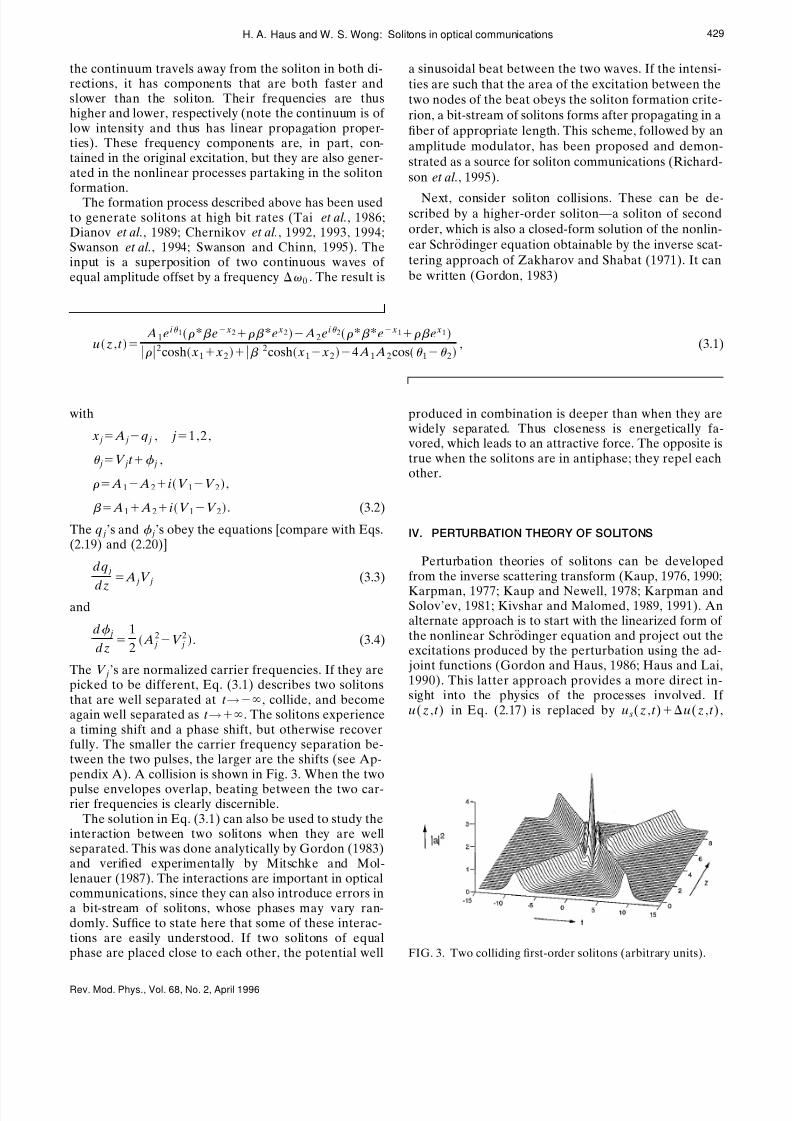
The V j ’s are normalized carrier frequencies. If they arepicked to be different, Eq. (3.1) describes two solitonsthat are well separated at t →, collide, and becomeagain well separated as t →. The solitons experiencea timing shift and a phase shift, but otherwise recoverfully. The smaller the carrier frequency separation be-tween the two pulses, the larger are the shifts (see Ap-pendix A). A collision is shown in Fig. 3. When the two

pulse envelopes overlap, beating between the two car-rier frequencies is clearly discernible.

The solution in Eq. (3.1) can also be used to study theinteraction between two solitons when they are wellseparated. This was done analytically by Gordon (1983)and verified experimentally by Mitschke and Mol-lenauer (1987). The interactions are important in opticalcommunications, since they can also introduce errors ina bit-stream of solitons, whose phases may vary ran-domly. Suffice to state here that some of these interac-tions are easily understood. If two solitons of equalphase are placed close to each other, the potential well

produced in combination is deeper than when they arewidely separated. Thus closeness is energetically fa-vored, which leads to an attractive force. The opposite istrue when the solitons are in antiphase; they repel eachother.

IV. PERTURBATION THEORY OF SOLITONS

Perturbation theories of solitons can be developedfrom the inverse scattering transform (Kaup, 1976, 1990;

Karpman, 1977; Kaup and Newell, 1978; Karpman andSolov’ev, 1981; Kivshar and Malomed, 1989, 1991). Analternate approach is to start with the linearized form of the nonlinear Schro ¨ dinger equation and project out theexcitations produced by the perturbation using the ad-

joint functions (Gordon and Haus, 1986; Haus and Lai,1990). This latter approach provides a more direct in-sight into the physics of the processes involved. If u(z ,t ) in Eq. (2.17) is replaced by u s(z ,t )u(z ,t ),

FIG. 3. Two colliding first-order solitons (arbitrary units).





where u(z ,t ) is the deviation of the field from the soli-ton solution u s(z, t ), the equation obeyed by u(z ,t ) tofirst order is

i

zuz, t

1

2

2

t 2uz ,t 2 u sz ,t 2uz, t

u s2z,t u*z ,t . (4.1)

This is a linear equation. Linear equations are solved by

finding their eigenfunctions and writing the solution as asuperposition of the eigenfunction excitations. The am-plitudes of the excitations are projected out using theorthogonality of the eigenfunctions, which is assuredprovided that the system is self-adjoint. Self-adjointnessis a natural consequence of energy conservation: solu-tions with different time dependences must be orthogo-nal, since if this were not the case, the energy would betime varying. Equation (4.1) is not self-adjoint. Eventhough the nonlinear Schro ¨ dinger equation is derivablefrom a Hamiltonian, the perturbation equation describesexcitations in the presence of a pump u s

2(z ,t ), andhence the energy of the perturbations need not be con-served. Orthogonality can be achieved with the solutionsof the adjoint equation whose solutions u(z,t ) obeycross-energy conservation:

d

dzRe

dt u*z ,t uz ,t 0. (4.2)

It is easily shown that the system adjoint to Eq. (4.1) is

i

zuz, t

1

2

2

t 2uz ,t 2 u sz ,t 2uz ,t

u s2z,t u*z ,t . (4.3)

Note the sign change in the last term. This sign changecorresponds to a 90° phase shift of the pump. In a para-metrically pumped system, such a phase shift switchesgrowing solutions to decaying solutions. If a solution of the system is growing, cross-energy is preserved whenthis solution is paired with the decaying solution of theadjoint system.

We write the perturbation as a superposition of changes in the four soliton parameters and of the con-tinuum [we use notation based on Gordon’s form of thesolution in Eq. (2.18)]:

uz ,t Az f A t z f t qz f q t

V z f V t e iz /2 e i ucz ,t , (4.4)

where uc(z ,t ) is the continuum. The four perturbationfunctions f P (t ) are derivatives of the soliton solutionwith respect to its four parameters P , where P A, ,q , and V , evaluated at z0:

f A t

Au s0,t 1t tanh t sech t ,

f t

u s0,t isech t ,

f q t

qu s0,t tanh t sech t ,

f V t

V u s0,t it sech t . (4.5)

With no loss of generality, the unperturbed solitonsolution has been assumed to have A1, 0, q0,V 0. The adjoint equation has similar solutions. Theyare orthonormal to the set in Eq. (4.5) and are found tobe

f A t sech t ,

f t i1t tanh t sech t ,

f q t t sech t ,

f V t itanh t sech t . (4.6)

The adjoint functions must be orthogonal to the con-tinuum. Indeed, as z→, the continuum is completelydispersed and has no overlap with the functions that oc-cupy the region around the soliton. Because of the con-

servation law, the orthogonality must hold for all z.When Eq. (4.4) is introduced into the governing equa-

tion (1), the second derivative of f A(t ) with respect totime produces a term proportional to f ( t ). This simplymeans that a change of amplitude causes a cumulativechange of phase, since the contribution from the Kerreffect has changed. Similarly, the second time derivativeof f V (t ) produces a term proportional to f q(t ); a changeof carrier frequency causes a cumulative change of dis-placement due to a change in group velocity. The per-turbation parameters are projected out by the four ad-

joint functions. This results in four equations of motionfor the soliton parameters:

d

dz AS Az, (4.7)

d

dz AS z , (4.8)

d

dzqV Sqz , (4.9)

d

dzV SV z, (4.10)

where the sources are given by

SP zRe

dtf P * t eiz /2 sz ,t , (4.11)

where s(z ,t ) represents a noise source added to theright-hand side of (4.1). These equations can, and will,be augmented to include filtering. They are sufficient toderive the Gordon-Haus effect. Before we proceed, wetake note of the fact that the perturbation analysis per-mits large changes of A, , q , and V , as long as





these changes are gradual and the generation of the con-tinuum is not excessive. Phase shifts, displacements, andfrequency shifts leave the soliton envelope unchanged.Even large amplitude changes may be incorporated if the projection functions in Eq. (4.5) are generalized toan arbitrary value of the amplitude A, as long as thesources SP (z) are evaluated at any cross section z con-sistently with the state of the soliton at that cross sec-tion. Then the parameters A, , q , and V areallowed to become large. We emphasize this fact bydropping the prefix henceforth and replacing A by

A1:

dA

dzS Az , (4.7a)

d

dz A1S z , (4.8a)

dq

dzV Sqz, (4.9a)

dV

dz SV z . (4.10a)

V. AMPLIFIER NOISE AND THE GORDON-HAUS EFFECT

We shall start with distributed gain that compensatesfor the fiber loss. Lumped gain is, of course, the practicalcase. We shall then consider the effects that are causedby lumped gain and ways to minimize them.

Suppose the normalized field gain coefficient is . If this gain compensates perfectly for the loss, Eq. (2.17)remains unchanged, assuming that noise can be ne-glected. However, in the case of long-distance propaga-tion with gains in the 100 dB range, amplifier noise can-not be neglected. It must be accounted for by adding asource term s(z, t ) Eqs. (2.17) and (4.1)—see Sec. VI forfurther discussion. If the amplifier bandwidth is muchlarger than the signal bandwidth, the source is character-ized by the correlation function (see Appendix B)

s*z ,t sz,t 2 N t t zz, (5.1)

where is amplitude gain per unit length and N is aparameter defined in Appendix B, Eq. (B8). Equation(5.1) is a delta function correlated in time, indicatingthat the noise is frequency independent. It is also a deltafunction correlated in space, since the gain and the as-sociated sources are due to gain media in different vol-

ume elements. Since the noise is described in terms of acorrelation function, the response must be similarly ex-pressed. The responses take the real part of complexprojections. This means that only the in-phase orquadrature (out of phase) components of the noise rep-resented by Eq. (5.1) contribute to any one of these pro-

jections. Since the noise is stationary, the in-phase andquadrature components have equal intensities, each withcorrelation functions equal to half the value of Eq. (5.1).The correlation function of the noise source in Eq.(4.10a), driving the velocity V (or normalized frequencydeviation), is

SV *zSV z N

dt

dt f V t f V * t

zz t t

N

dt tanh2 t sech2 t zz

2

3 N zz. (5.2)

The noise source driving the displacement q (note that A1) is

Sq*z Sqz N

dt

dt f q t f q* t

zz t t

N

dtt 2sech2 t zz

2

6 N zz. (5.3)

The correlation function of the velocity (or normalizedfrequency deviation) is

V *z V z 0

z

dzSV *z0

zdzSV z

2 N

3

0

zdz

2 N

3z for zz

2 N 3

z for zz

.

(5.4)

The mean square fluctuations of the displacement areproduced by frequency fluctuations on the one hand andby a noise source driving the displacement directly onthe other hand. Since the two noise sources are indepen-dent, the mean-square fluctuations that they produce areadditive. Considering first the mean-square fluctuationsdue to the noise source Sq(z), we have, in analogy withEq. (5.4),

q*L qL q 0

L

dzSq*z0

L

dzSqz

2 N

6

0

L

dz 2 N

6L, (5.5)

where L is the distance of propagation. These mean-square fluctuations grow linearly with L. They corre-spond to a simple random walk of the displacement vari-able. The mean-square fluctuations caused by thefrequency fluctuations are





q*L qLV 0

L

dzV *z0

L

dzV z

2 N

32

0

L

dz0

zzdz

2 N

3

L3

3. (5.6)

From Eq. (5.4), we see that the frequency fluctuationsexperience a random walk (linear growth with L), whichis translated into a much larger growth of the displace-ment, since pulses with different carrier frequenciestravel at different speeds; this effect becomes severe forlarge distances of propagation. The mean-square fluc-tuations grow with the cube of the distance. For largepropagation distances they dominate. This is the socalled Gordon-Haus effect (Gordon and Haus, 1986). Itleads to random displacements of pulses that may endup in neighboring time slots, causing bit errors.

The analysis thus far has been in normalized units.

The standard soliton was sech( t ), where the normaliza-tion time n was equal to the pulse width . The mean-square displacement fluctuations q*(L)q(L) werenormalized to the pulse width. The bit-error rate can becomputed from them directly once the pulse-width tobit-interval ratio is chosen. The right-hand side of Eq.(5.6) is converted to physical dimensions as follows:

q*L qLV 2 znN

3

L3/zn3

3

2 zn

3

0

An2 n

L3/zn3

3; (5.7)

the parameter (1) expresses imperfect inversion of the gain medium, and zn is a normalized distance scale.Using zn / n

21 and An2zn1, one can write the

above as

q*L qLV

2

3 0

L3

3 3. (5.8)

The effect is proportional to the Kerr coefficient , in-dicating that the jitter is Kerr-induced. The jitter in-creases with the cube of the distance and is proportionalto the GVD. Reducing the GVD reduces the effect andthis fact is used in the design of the fiber. Since the bitrate is proportional to 1/ , we find that the jitter in-

creases with the cube of the bit rate. For given fiberparameters and a fixed bit rate, the energy of the pulse isgiven by

w2 A02 2

. (5.9)

We find that, changing the power level of transmission,the fluctuations scale as the cube of the power (or en-ergy):

q*L qLV

2

3 0

L3

3 w

2 3

. (5.10)

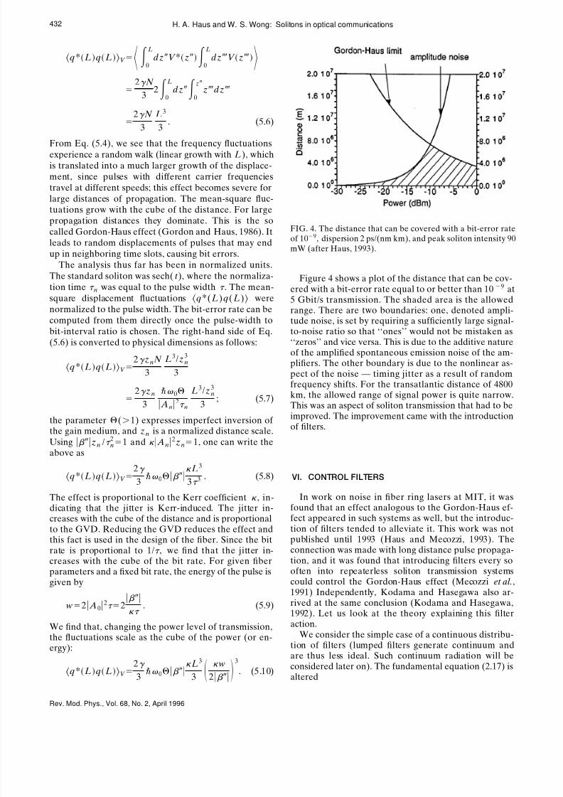
Figure 4 shows a plot of the distance that can be cov-ered with a bit-error rate equal to or better than 109 at5 Gbit/s transmission. The shaded area is the allowedrange. There are two boundaries: one, denoted ampli-tude noise, is set by requiring a sufficiently large signal-to-noise ratio so that ‘‘ones’’ would not be mistaken as‘‘zeros’’ and vice versa. This is due to the additive natureof the amplified spontaneous emission noise of the am-plifiers. The other boundary is due to the nonlinear as-pect of the noise — timing jitter as a result of randomfrequency shifts. For the transatlantic distance of 4800km, the allowed range of signal power is quite narrow.This was an aspect of soliton transmission that had to be

improved. The improvement came with the introductionof filters.

VI. CONTROL FILTERS

In work on noise in fiber ring lasers at MIT, it wasfound that an effect analogous to the Gordon-Haus ef-fect appeared in such systems as well, but the introduc-tion of filters tended to alleviate it. This work was notpublished until 1993 (Haus and Mecozzi, 1993). Theconnection was made with long distance pulse propaga-

tion, and it was found that introducing filters every sooften into repeaterless soliton transmission systemscould control the Gordon-Haus effect (Mecozzi et al.,1991) Independently, Kodama and Hasegawa also ar-rived at the same conclusion (Kodama and Hasegawa,1992). Let us look at the theory explaining this filteraction.

We consider the simple case of a continuous distribu-tion of filters (lumped filters generate continuum andare thus less ideal. Such continuum radiation will beconsidered later on). The fundamental equation (2.17) isaltered

FIG. 4. The distance that can be covered with a bit-error rateof 109, dispersion 2 ps/(nm km), and peak soliton intensity 90mW (after Haus, 1993).





i

zuz, t

1

2

2

t 2uz ,t uz ,t 2uz ,t

i1

f 2

2

t 2uz ,t sz, t , (6.1)

where 1/ f 2 expresses the filtering per unit (normalized)

distance, and where we have included the noise source s(z ,t ). The soliton perturbation equation changes ac-cordingly:

i

zuz, t

1

2

2

t 2uz ,t 2 u sz ,t 2uz, t

u s2z,t u*z ,t

i1

f 2

2

t 2u sz ,t sz, t . (6.2)

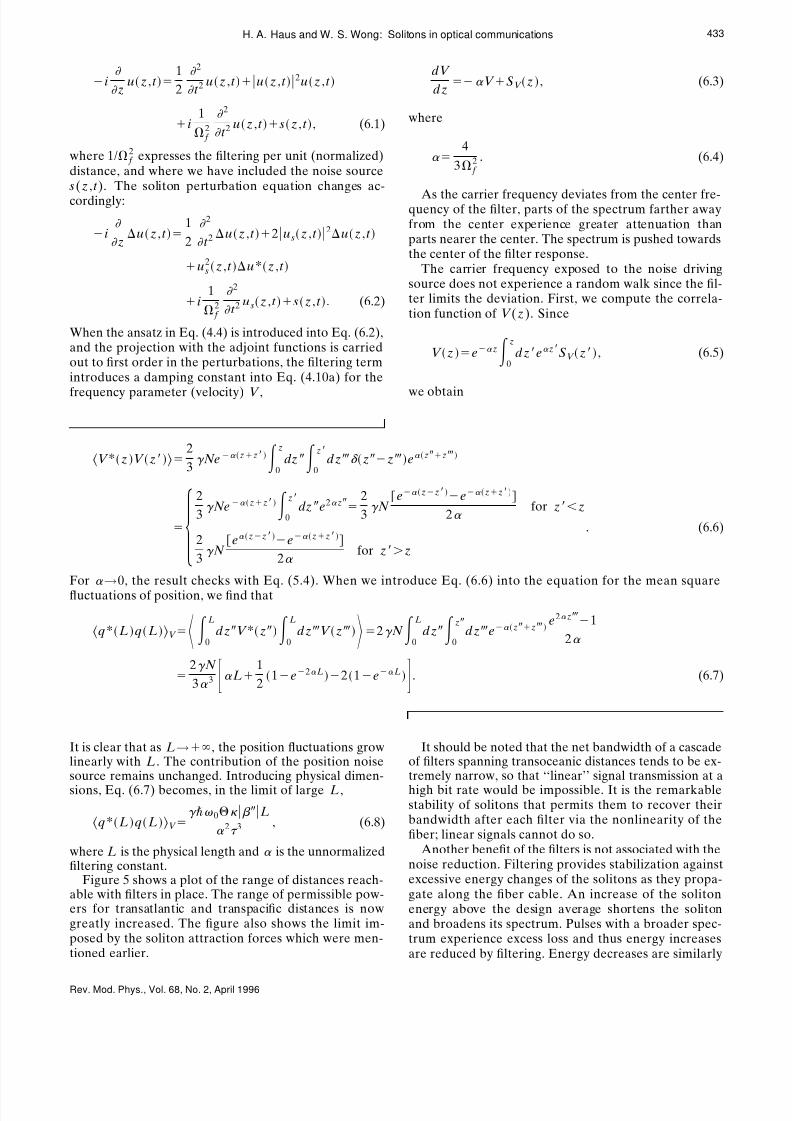
When the ansatz in Eq. (4.4) is introduced into Eq. (6.2),and the projection with the adjoint functions is carriedout to first order in the perturbations, the filtering termintroduces a damping constant into Eq. (4.10a) for the

frequency parameter (velocity) V ,

dV

dz V SV z , (6.3)

where

4

3 f 2 . (6.4)

As the carrier frequency deviates from the center fre-quency of the filter, parts of the spectrum farther awayfrom the center experience greater attenuation thanparts nearer the center. The spectrum is pushed towardsthe center of the filter response.

The carrier frequency exposed to the noise drivingsource does not experience a random walk since the fil-ter limits the deviation. First, we compute the correla-tion function of V (z). Since

V z e z0

z

dze zSV z, (6.5)

we obtain

V *z V z2

3 Ne zz

0

z

dz 0

zdz zze zz

2

3 Ne zz

0

zdz e2 z

2

3 N

e zze zz

2 for zz

2

3 N

e zze zz

2 for zz

. (6.6)

For →0, the result checks with Eq. (5.4). When we introduce Eq. (6.6) into the equation for the mean squarefluctuations of position, we find that

q*L qLV 0

L

dzV *z0

L

dzV z2 N 0

L

dz0

zdze zz

e2 z1

2

2 N

3 3 L 1

21e2 L21e L . (6.7)

It is clear that as L→, the position fluctuations growlinearly with L. The contribution of the position noisesource remains unchanged. Introducing physical dimen-sions, Eq. (6.7) becomes, in the limit of large L,

q*L qLV 0 L

2 3, (6.8)

where L is the physical length and is the unnormalizedfiltering constant.

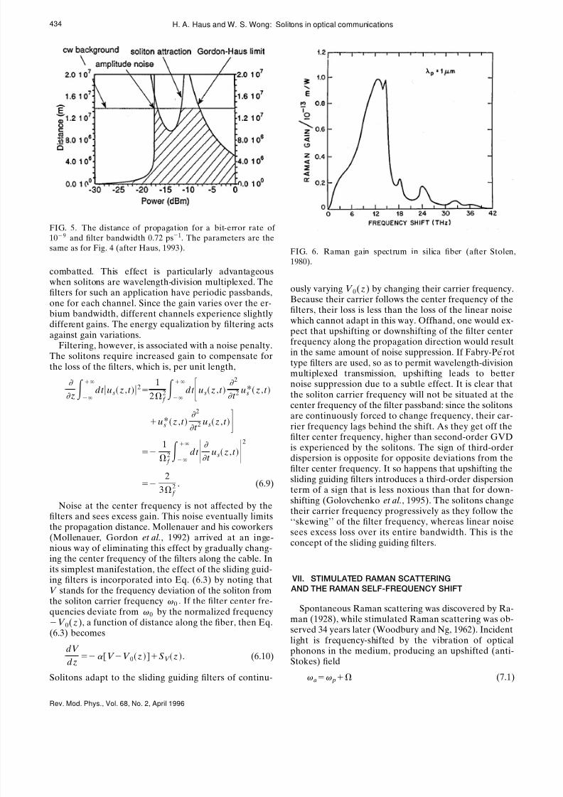
Figure 5 shows a plot of the range of distances reach-able with filters in place. The range of permissible pow-ers for transatlantic and transpacific distances is nowgreatly increased. The figure also shows the limit im-posed by the soliton attraction forces which were men-tioned earlier.

It should be noted that the net bandwidth of a cascadeof filters spanning transoceanic distances tends to be ex-tremely narrow, so that ‘‘linear’’ signal transmission at ahigh bit rate would be impossible. It is the remarkablestability of solitons that permits them to recover theirbandwidth after each filter via the nonlinearity of thefiber; linear signals cannot do so.

Another benefit of the filters is not associated with thenoise reduction. Filtering provides stabilization againstexcessive energy changes of the solitons as they propa-gate along the fiber cable. An increase of the solitonenergy above the design average shortens the solitonand broadens its spectrum. Pulses with a broader spec-trum experience excess loss and thus energy increasesare reduced by filtering. Energy decreases are similarly





combatted. This effect is particularly advantageous

when solitons are wavelength-division multiplexed. Thefilters for such an application have periodic passbands,one for each channel. Since the gain varies over the er-bium bandwidth, different channels experience slightlydifferent gains. The energy equalization by filtering actsagainst gain variations.

Filtering, however, is associated with a noise penalty.The solitons require increased gain to compensate forthe loss of the filters, which is, per unit length,

z

dt u sz, t 2

1

2 f 2

dt u sz ,t 2

t 2u s*z, t

u s*z ,t

2

t 2u sz, t

1

f 2

dt t

u sz, t 2

2

3 f 2 . (6.9)

Noise at the center frequency is not affected by thefilters and sees excess gain. This noise eventually limitsthe propagation distance. Mollenauer and his coworkers(Mollenauer, Gordon et al., 1992) arrived at an inge-nious way of eliminating this effect by gradually chang-

ing the center frequency of the filters along the cable. Inits simplest manifestation, the effect of the sliding guid-ing filters is incorporated into Eq. (6.3) by noting thatV stands for the frequency deviation of the soliton fromthe soliton carrier frequency 0 . If the filter center fre-quencies deviate from 0 by the normalized frequencyV 0(z), a function of distance along the fiber, then Eq.(6.3) becomes

dV

dz V V 0z SV z . (6.10)

Solitons adapt to the sliding guiding filters of continu-

ously varying V 0(z) by changing their carrier frequency.Because their carrier follows the center frequency of thefilters, their loss is less than the loss of the linear noisewhich cannot adapt in this way. Offhand, one would ex-pect that upshifting or downshifting of the filter centerfrequency along the propagation direction would resultin the same amount of noise suppression. If Fabry-Pe rottype filters are used, so as to permit wavelength-divisionmultiplexed transmission, upshifting leads to betternoise suppression due to a subtle effect. It is clear thatthe soliton carrier frequency will not be situated at thecenter frequency of the filter passband: since the solitons

are continuously forced to change frequency, their car-rier frequency lags behind the shift. As they get off thefilter center frequency, higher than second-order GVDis experienced by the solitons. The sign of third-orderdispersion is opposite for opposite deviations from thefilter center frequency. It so happens that upshifting thesliding guiding filters introduces a third-order dispersionterm of a sign that is less noxious than that for down-shifting (Golovchenko et al., 1995). The solitons changetheir carrier frequency progressively as they follow the‘‘skewing’’ of the filter frequency, whereas linear noisesees excess loss over its entire bandwidth. This is theconcept of the sliding guiding filters.

VII. STIMULATED RAMAN SCATTERING

AND THE RAMAN SELF-FREQUENCY SHIFT

Spontaneous Raman scattering was discovered by Ra-man (1928), while stimulated Raman scattering was ob-served 34 years later (Woodbury and Ng, 1962). Incidentlight is frequency-shifted by the vibration of opticalphonons in the medium, producing an upshifted (anti-Stokes) field

a p (7.1)

FIG. 5. The distance of propagation for a bit-error rate of 109 and filter bandwidth 0.72 ps1. The parameters are thesame as for Fig. 4 (after Haus, 1993). FIG. 6. Raman gain spectrum in silica fiber (after Stolen,

1980).





and a downshifted (Stokes) field

s p, (7.2)

where p is the frequency of the incoming photon and is the optical phonon frequency.

Stolen and his coworkers first observed stimulatedRaman scattering in an optical fiber and measured theRaman gain spectrum (Stolen et al., 1972; Stolen andIppen, 1973). Because silica glass is amorphous, the pho-non frequency becomes a continuum and significantlybroadens the gain spectrum, which peaks at 13 THz andspans 40 THz (Fig. 6). In the first soliton transmissionexperiment, Mollenauer used the Raman gain to com-pensate for losses in the fiber (Mollenauer and Smith,1988).

Gordon found that for very short solitons, the pulsespectrum can be so broad that the blue part of the spec-trum can act as a pump for the stimulated Raman pro-cess to amplify the red part of the spectrum. If left un-checked, the mean frequency of solitons is continuouslydownshifted (Gordon, 1986). This effect, verified experi-mentally by Mitschke and Mollenauer (1986), is known

as the Raman self-frequency shift, which can be mod-eled by including an additional term in the nonlinearSchro ¨ dinger equation (Kodama and Hasegawa, 1987).The Kerr coefficient n2 becomes frequency dependentwhen the exciting signal is broadband. If the pumpingsignals have frequencies and , respectively, n2

must be replaced by

n2 n20

1i K

, (7.3)

where K is the Kerr relaxation rate. Note that n2( )becomes complex. The system is capable of gain, namelyRaman gain: low frequencies are amplified at the ex-

pense of high frequencies. Our model for n2 is adequateto describe Raman gain for frequencies close to thepump frequency. The phase shift in Eq. (2.8) becomes,to first order in frequency difference:

n20

d

d 1i K

vz, v*z , vz, . (7.4)

When transformed into the time domain, the result is

n20 vz, t 2 K

t vz, t 2vz ,t . (7.5)

A perturbation term must be introduced into the nor-malized nonlinear Schro ¨ dinger equation:

i

zuz, t

1

2

2

t 2uz ,t uz ,t 2uz ,t

cR K

n

uz ,t 2

t uz, t , (7.6)

where c R K is the effective Raman response timeweighted by the shape of the gain spectrum (Gordon,1986).

In addition to the noise-imparted velocity fluctuations

in the Gordon-Haus effect, there are photon-numberfluctuations as well, which are commensurate with pulse-width fluctuations as a result of the area theorem. Afluctuation in photon number or in pulse width alters therate of Raman self-frequency shifting of a soliton. This isanalogous to a changing deceleration. When integratingover long distances, it was found that the Raman timingfluctuations grow with the fifth power of distance, andmay exceed the Gordon-Haus jitter at high bit rates(Wood, 1990; Nakazawa, Kubota et al., 1991; Mooreset al., 1994; Qiu, 1994).

VIII. CONTINUUM GENERATION

A lumped disturbance, such as an amplifier, not onlycauses a perturbation of the soliton, but also generatescontinuum. In fact, if one separates Eq. (4.4) into twoparts, one associated with the soliton, the other with thecontinuum, the result is

uz ,t Az f A t z f t qz f q t

V z f V t eiz /2

ei

ucz ,t

u sz ,t ucz ,t , (8.1)

in which one can distinguish between the excitation of the continuum uc and the perturbation of the solitonu s . Suppose that a sudden change u(0,t ) is caused atz0. Then the continuum part of this change is

uc0,t u0,t P

Re

dtf P * t u0,t .

(8.2)

The excitation of the continuum is particularly severewhen a periodic perturbation approaches phase-

matched conditions (Gordon, 1992; Kelly, 1992; Materaet al., 1993). This condition is illustrated in Fig. 7. Theordinate is 1

2 2 , the abscissa is the frequency devia-

tion . The parabola shows the dispersion of the linearwaves. The propagation constant of the continuum, alinear excitation, follows the parabola. The soliton has apropagation constant corresponding to 0 supple-mented by the Kerr phase shift of 1/2 in normalizedunits. The spectrum of the soliton is shown on the samegraph. If the normalized distance of the periodic pertur-bation is L, then the periodic perturbation can phasematch the soliton spectrum to the continuum at two spe-cific frequencies as shown. Excitation of the continuum

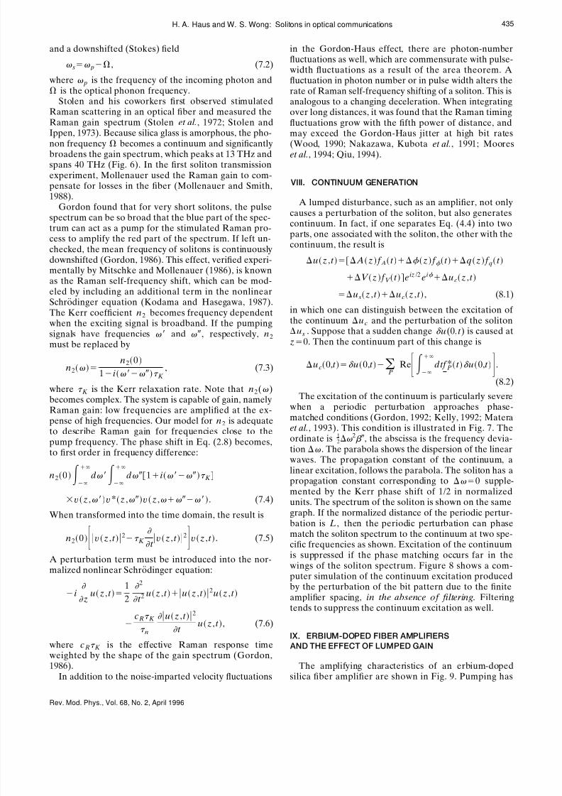
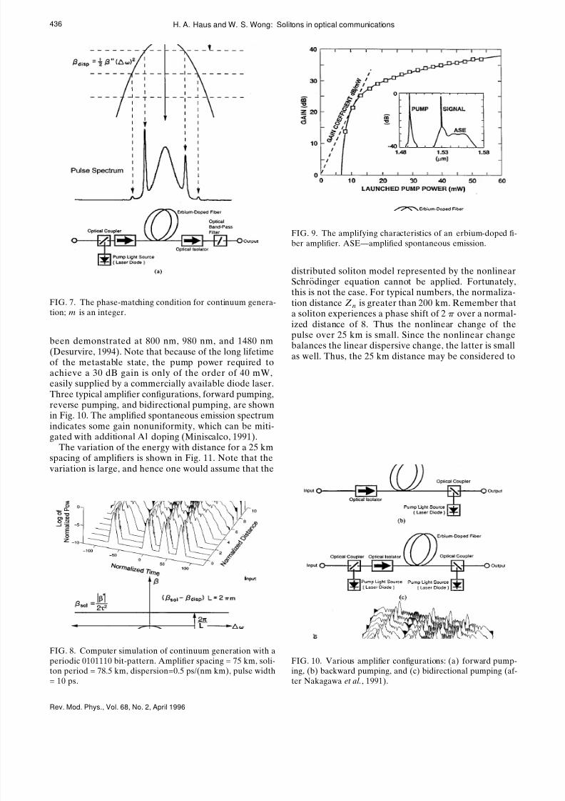
is suppressed if the phase matching occurs far in thewings of the soliton spectrum. Figure 8 shows a com-puter simulation of the continuum excitation producedby the perturbation of the bit pattern due to the finiteamplifier spacing, in the absence of filtering. Filteringtends to suppress the continuum excitation as well.

IX. ERBIUM-DOPED FIBER AMPLIFIERS

AND THE EFFECT OF LUMPED GAIN

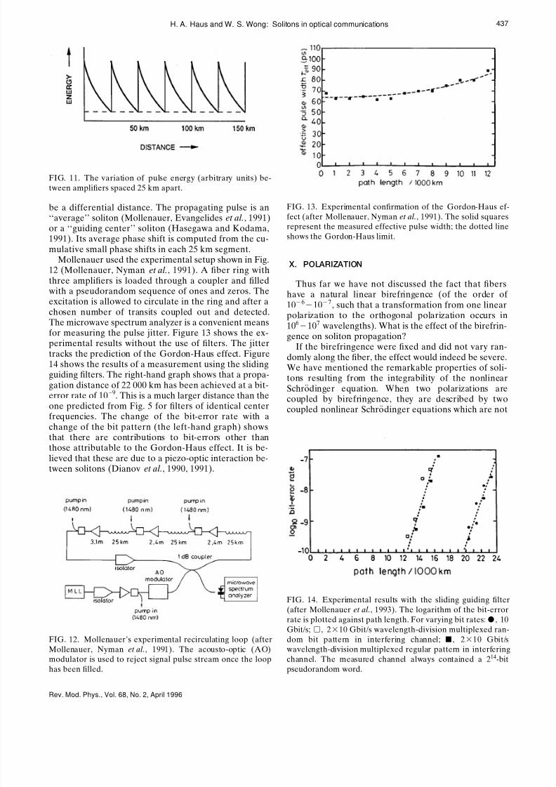
The amplifying characteristics of an erbium-dopedsilica fiber amplifier are shown in Fig. 9. Pumping has





been demonstrated at 800 nm, 980 nm, and 1480 nm(Desurvire, 1994). Note that because of the long lifetimeof the metastable state, the pump power required toachieve a 30 dB gain is only of the order of 40 mW,easily supplied by a commercially available diode laser.Three typical amplifier configurations, forward pumping,reverse pumping, and bidirectional pumping, are shownin Fig. 10. The amplified spontaneous emission spectrumindicates some gain nonuniformity, which can be miti-gated with additional Al doping (Miniscalco, 1991).

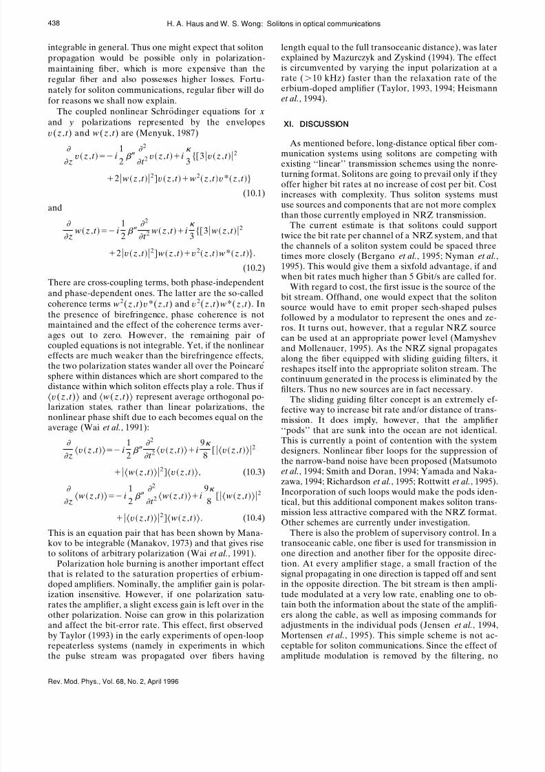
The variation of the energy with distance for a 25 kmspacing of amplifiers is shown in Fig. 11. Note that thevariation is large, and hence one would assume that the

distributed soliton model represented by the nonlinear

Schro ¨ dinger equation cannot be applied. Fortunately,this is not the case. For typical numbers, the normaliza-tion distance Z n is greater than 200 km. Remember thata soliton experiences a phase shift of 2 over a normal-ized distance of 8. Thus the nonlinear change of thepulse over 25 km is small. Since the nonlinear changebalances the linear dispersive change, the latter is smallas well. Thus, the 25 km distance may be considered to

FIG. 7. The phase-matching condition for continuum genera-tion; m is an integer.

FIG. 8. Computer simulation of continuum generation with aperiodic 0101110 bit-pattern. Amplifier spacing = 75 km, soli-ton period = 78.5 km, dispersion=0.5 ps/(nm km), pulse width= 10 ps.

FIG. 9. The amplifying characteristics of an erbium-doped fi-ber amplifier. ASE—amplified spontaneous emission.

FIG. 10. Various amplifier configurations: (a) forward pump-ing, (b) backward pumping, and (c) bidirectional pumping (af-ter Nakagawa et al., 1991).





be a differential distance. The propagating pulse is an‘‘average’’ soliton (Mollenauer, Evangelides et al., 1991)or a ‘‘guiding center’’ soliton (Hasegawa and Kodama,1991). Its average phase shift is computed from the cu-mulative small phase shifts in each 25 km segment.

Mollenauer used the experimental setup shown in Fig.12 (Mollenauer, Nyman et al., 1991). A fiber ring withthree amplifiers is loaded through a coupler and filledwith a pseudorandom sequence of ones and zeros. Theexcitation is allowed to circulate in the ring and after achosen number of transits coupled out and detected.The microwave spectrum analyzer is a convenient meansfor measuring the pulse jitter. Figure 13 shows the ex-perimental results without the use of filters. The jittertracks the prediction of the Gordon-Haus effect. Figure14 shows the results of a measurement using the slidingguiding filters. The right-hand graph shows that a propa-gation distance of 22 000 km has been achieved at a bit-error rate of 10−9. This is a much larger distance than theone predicted from Fig. 5 for filters of identical center

frequencies. The change of the bit-error rate with achange of the bit pattern (the left-hand graph) showsthat there are contributions to bit-errors other thanthose attributable to the Gordon-Haus effect. It is be-lieved that these are due to a piezo-optic interaction be-tween solitons (Dianov et al., 1990, 1991).

X. POLARIZATION

Thus far we have not discussed the fact that fibershave a natural linear birefringence (of the order of 106

107, such that a transformation from one linearpolarization to the orthogonal polarization occurs in106107 wavelengths). What is the effect of the birefrin-

gence on soliton propagation?If the birefringence were fixed and did not vary ran-

domly along the fiber, the effect would indeed be severe.We have mentioned the remarkable properties of soli-tons resulting from the integrability of the nonlinearSchro ¨ dinger equation. When two polarizations arecoupled by birefringence, they are described by two

coupled nonlinear Schro ¨

dinger equations which are not

FIG. 11. The variation of pulse energy (arbitrary units) be-tween amplifiers spaced 25 km apart.

FIG. 12. Mollenauer’s experimental recirculating loop (afterMollenauer, Nyman et al., 1991). The acousto-optic (AO)modulator is used to reject signal pulse stream once the loophas been filled.

FIG. 13. Experimental confirmation of the Gordon-Haus ef-fect (after Mollenauer, Nyman et al., 1991). The solid squaresrepresent the measured effective pulse width; the dotted lineshows the Gordon-Haus limit.

FIG. 14. Experimental results with the sliding guiding filter(after Mollenauer et al., 1993). The logarithm of the bit-errorrate is plotted against path length. For varying bit rates: , 10Gbit/s; , 210 Gbit/s wavelength-division multiplexed ran-dom bit pattern in interfering channel; , 210 Gbit/swavelength-division multiplexed regular pattern in interferingchannel. The measured channel always contained a 214-bitpseudorandom word.





integrable in general. Thus one might expect that solitonpropagation would be possible only in polarization-maintaining fiber, which is more expensive than theregular fiber and also possesses higher losses. Fortu-nately for soliton communications, regular fiber will dofor reasons we shall now explain.

The coupled nonlinear Schro ¨ dinger equations for x

and y polarizations represented by the envelopes

v(z ,t ) and w(z ,t ) are (Menyuk, 1987)

zvz, t i

1

2

2

t 2vz, t i

33 vz, t 2

2wz, t 2vz ,t w2z ,t v*z ,t

(10.1)

and

zwz ,t i

1

2

2

t 2wz ,t i

33wz, t 2

2 vz, t 2wz ,t v2z ,t w*z ,t .

(10.2)There are cross-coupling terms, both phase-independentand phase-dependent ones. The latter are the so-calledcoherence terms w2(z ,t )v*(z ,t ) and v

2(z ,t )w*(z ,t ). Inthe presence of birefringence, phase coherence is notmaintained and the effect of the coherence terms aver-ages out to zero. However, the remaining pair of coupled equations is not integrable. Yet, if the nonlineareffects are much weaker than the birefringence effects,the two polarization states wander all over the Poincare

sphere within distances which are short compared to thedistance within which soliton effects play a role. Thus if v(z, t ) and w(z, t ) represent average orthogonal po-

larization states, rather than linear polarizations, thenonlinear phase shift due to each becomes equal on theaverage (Wai et al., 1991):

zvz ,t i

1

2

2

t 2vz, t i

9

8 vz ,t 2

wz ,t 2vz, t , (10.3)

zwz ,t i

1

2

2

t 2wz ,t i

9

8 wz ,t 2

vz ,t 2wz ,t . (10.4)

This is an equation pair that has been shown by Mana-

kov to be integrable (Manakov, 1973) and that gives riseto solitons of arbitrary polarization (Wai et al., 1991).

Polarization hole burning is another important effectthat is related to the saturation properties of erbium-doped amplifiers. Nominally, the amplifier gain is polar-ization insensitive. However, if one polarization satu-rates the amplifier, a slight excess gain is left over in theother polarization. Noise can grow in this polarizationand affect the bit-error rate. This effect, first observedby Taylor (1993) in the early experiments of open-looprepeaterless systems (namely in experiments in whichthe pulse stream was propagated over fibers having

length equal to the full transoceanic distance), was laterexplained by Mazurczyk and Zyskind (1994). The effectis circumvented by varying the input polarization at arate (10 kHz) faster than the relaxation rate of theerbium-doped amplifier (Taylor, 1993, 1994; Heismannet al., 1994).

XI. DISCUSSION

As mentioned before, long-distance optical fiber com-munication systems using solitons are competing withexisting ‘‘linear’’ transmission schemes using the nonre-turning format. Solitons are going to prevail only if theyoffer higher bit rates at no increase of cost per bit. Costincreases with complexity. Thus soliton systems mustuse sources and components that are not more complexthan those currently employed in NRZ transmission.

The current estimate is that solitons could supporttwice the bit rate per channel of a NRZ system, and thatthe channels of a soliton system could be spaced threetimes more closely (Bergano et al., 1995; Nyman et al.,

1995). This would give them a sixfold advantage, if andwhen bit rates much higher than 5 Gbit/s are called for.With regard to cost, the first issue is the source of the

bit stream. Offhand, one would expect that the solitonsource would have to emit proper sech-shaped pulsesfollowed by a modulator to represent the ones and ze-ros. It turns out, however, that a regular NRZ sourcecan be used at an appropriate power level (Mamyshevand Mollenauer, 1995). As the NRZ signal propagatesalong the fiber equipped with sliding guiding filters, itreshapes itself into the appropriate soliton stream. Thecontinuum generated in the process is eliminated by thefilters. Thus no new sources are in fact necessary.

The sliding guiding filter concept is an extremely ef-fective way to increase bit rate and/or distance of trans-mission. It does imply, however, that the amplifier‘‘pods’’ that are sunk into the ocean are not identical.This is currently a point of contention with the systemdesigners. Nonlinear fiber loops for the suppression of the narrow-band noise have been proposed (Matsumotoet al., 1994; Smith and Doran, 1994; Yamada and Naka-zawa, 1994; Richardson et al., 1995; Rottwitt et al., 1995).Incorporation of such loops would make the pods iden-tical, but this additional component makes soliton trans-mission less attractive compared with the NRZ format.Other schemes are currently under investigation.

There is also the problem of supervisory control. In a

transoceanic cable, one fiber is used for transmission inone direction and another fiber for the opposite direc-tion. At every amplifier stage, a small fraction of thesignal propagating in one direction is tapped off and sentin the opposite direction. The bit stream is then ampli-tude modulated at a very low rate, enabling one to ob-tain both the information about the state of the amplifi-ers along the cable, as well as imposing commands foradjustments in the individual pods (Jensen et al., 1994,Mortensen et al., 1995). This simple scheme is not ac-ceptable for soliton communications. Since the effect of amplitude modulation is removed by the filtering, no





low-level signal can be returned in the fiber carrying thebit stream in the opposite direction. Thus, the supervi-sory control in a soliton system is an important issue thathas to be settled.

In conclusion one may state that repeaterless propa-gation of signals via solitons has made enormousprogress in recent years. It is an example of a rapid de-ployment of a sophisticated physical phenomenon forpractical use. The work on soliton transmission hasspurred on the development of ‘‘linear’’ NRZ repeater-less optical fiber transmission, which has already beendeployed. The deployment of soliton optical fiber trans-mission will be dependent on overcoming the stiff com-petition presented by the NRZ systems.

ACKNOWLEDGMENTS

This research was supported in part by the U.S. Navy/Office of Naval Research under contract N00014–92–J–

1302, the Joint Services Electronics Program under con-tract DAAH04–95–1–0038, and the U.S. Air ForceOffice of Scientific Research under contract F49620–95–1–0021. The authors wish to thank F. I. Khatri for gen-erating Fig. 8. Computing resources were made availableto us from the San Diego Supercomputing Center.

APPENDIX A: SOLITON COLLISION EFFECTS

When two solitons pass each other, they shift eachother’s position and phase, while their carrier frequen-cies and amplitudes remain unaffected. This can beshown with the aid of the second order soliton solutionin Eq. (3.1):

uz ,t A1e i 1 * e x2 *e x2 A2e i 2 * *e x1 e x1 2cosh x1 x2 2cosh x1 x24 A1 A2cos 1 2

. (A1)

If the velocities satisfy V 2V 1 , then the positions obeyq2q1 for z→, and q2q1 for z→. With in-creasing z , soliton (2) starts out ahead of soliton (1) andends up behind it. One can extricate soliton (1) from Eq.(A1) in the two limits by setting e x20 when z→,and e x2 when z→. One obtains from Eq. (A1),

u2 A1e i 1 *

2e

x1 2e x1 forz→

2 A 1e i 1 *

2e x1 2e x1for z→

. (A2)

These two expressions are hyperbolic secants that aremutually shifted by

q2ln

ln

A 1 A22V 1V 2

2

A1 A 22V 1V 2

2 . (A3)

The net phase shift is

2arg 2arg

2tan

1V 1V 2

A 1 A22tan

1V 1V 2

A1 A2 . (A4)

Note that the maximum phase shift is , when A1 A2 .

APPENDIX B: THE AMPLIFIED SPONTANEOUS EMISSION

NOISE SOURCE

Amplified spontaneous emission is represented by adistributed noise source. The propagation of the ampli-tude a(z, ) of a mode in the single-mode fiber experi-encing gain is described by

zaz , az , nz , , (B1)

where is the amplitude gain per unit length andn(z , ) is the noise source: this is a delta function cor-related from segment to segment, since the noise sourcesin different volume elements are independent:

n*z , nz, C zz. (B2)

The magnitude of C is determined from the well-knownresult that the amplified spontaneous emission output-power spectral density of an amplifier of length L withpower gain Gexp(2 L) is

a*L, aL, 1

2 0G1. (B3)

Here 0 is the nominal center frequency of the ampli-fier. The gain is assumed to be uniform over the band-width of interest and then the noise spectral density isfrequency independent. The parameter (1) ex-presses imperfect inversion of the gain medium. In anondegenerate two level system, n2 /(n2n1),where n1 and n2 are the populations of the lower andthe upper level, respectively. For an erbium-doped fiberamplifer pumped at a wavelength of 980 nm, 2.

Returning to Eq. (B1) and integrating it to find theoutput spectral density, one obtains





a*L, aL, exp2 L0

L

dzexp z0

L

dz

exp zn*z, nz,

C exp2 L 0

L

dz exp z

0

L

dzexp z z

z

C exp2 L 1

2

C

2 G1

0

2 G1. (B4)

In this way the noise source is found to be

n*z , nz, 2 01

2 zz. (B5)

In the time domain one obtains for the autocorrelation

functionn*z ,t nz, t 2 0 zz t t . (B6)

If the normalizations of the distance variable, timevariable, and amplitude are introduced into Eq. (B6),the autocorrelation of the noise source s(z ,t ) is

s*z,t sz, t 2 0zn

A n2 n zz t t

2 zn

0

An2 n zz

zn t t

n

→2 N zz t t , (B7)

where

N Z n

An2 n(B8)

and where it should be noted that, in the transition fromthe next-to-last to the last expression, the spatial andtime variables have been replaced by their normalizedversions without a change of notation (as done in thetext). This is indicated by an arrow, rather than anequality sign.

REFERENCES

Agrawal, G. P., 1989, Nonlinear Fiber Optics (Academic Press,San Diego, CA).

Andrekson, P. A., N. A. Olsson, M. Haner, J. R. Simpson, T.Tanbun-Ek, R. A. Logan, D. Coblentz, H. M. Presby, and K.W. Wecht, 1992, ‘‘32 Gb/s optical soliton data transmissionover 90 km,’’ IEEE Photonics Technol. Lett. 4, 76–79.

Aubin, G., E. Jeanney, T. Montalant, J. Moulu, F. Pirio, J.-B.Thomine, and F. Devaux, 1995, ‘‘20 Gbit/s soliton transmis-sion over transoceanic distances with a 105 km amplifierspan,’’ Electron. Lett. 31, 1079–1080.

Aubin, G., T. Montalant, J. Moulu, B. Nortier, F. Pirio, and J.

Thomine, 1994, ‘‘Soliton transmission at 10 Gbit/s with a 70

km amplifier span over one million kilometres,’’ Electron.

Lett. 30, 1163–1165.

Aubin, G., T. Montalant, J. Moulu, B. Nortier, F. Pirio, and

J.-B. Thomine, 1995a, ‘‘Demonstration of soliton transmis-

sion at 10 Gbit/s up to 27 Mm using ‘signal frequency sliding’

technique,’’ Electron. Lett. 31, 52–53.

Aubin, G., T. Montalant, J. Moulu, B. Nortier, F. Pirio, and

J.-B. Thomine, 1995b, ‘‘Record amplifier span of 105 km in a

soliton transmission experiment at 10 Gbit/s over 1 Mm,’’Electron. Lett. 31, 217–219.

Bergano, N. S., and C. R. Davidson, 1995, ‘‘Circulating looptransmission experiments for the study of long-haul transmis-sion systems using erbium-doped fiber amplifiers,’’ J. Light-wave Technol. 13, 879–888.

Bergano, N. S., et al., 1995, ‘‘40 Gb/s WDM transmission of eight 5 Gb/s data channels over transoceanic distances usingthe conventional NRZ modulation format,’’ in OFC’95, opti-

cal fiber communication: summaries of papers presented at the

Conference on Optical Fiber Communication, San Diego,

California, 1995 Technical Digest Series, Vol. 8 (Optical So-

ciety of America, Washington, D.C.), p. PD19.Butler, D. J., K. P. Jones, and V. Syngal, 1994, ‘‘10 Gbit/stransmission by two channel WDM over a 980 km, sevenoptical amplifier line,’’ Electron. Lett. 30, 249–251.

Chernikov, S. V., D. J. Richardson, R. I. Laming, E. M. Di-anov, and D. N. Payne, 1992, ‘‘70 Gbit/s fibre based source of fundamental solitons at 1550 nm,’’ Electron. Lett. 28, 1210–1212.

Chernikov, S. V., J. R. Taylor, and R. Kashyap, 1993, ‘‘Inte-grated all optical fibre source of multigigahertz soliton pulsetrain,’’ Electron. Lett. 29, 1788–1789.

Chernikov, S. V., J. R. Taylor, and R. Kashyap, 1994, ‘‘Experi-mental demonstration of step-like dispersion profiling in op-tical fibre for soliton pulse generation and compression,’’

Electron. Lett. 30, 433–435.Clesca, B., C. Cœurjolly, D. Bayart, L. Berthelon, L. Hamon,and J. L. Beylat, 1994, ‘‘Experimental demonstration of thefeasibility of 40 Gbit/s transmission through 440 km standardfibre,’’ Electron. Lett. 30, 802–803.

Desurvire, E., J. R. Simpson, and P. C. Pecker, 1987, ‘‘High-gain erbium-doped traveling-wave fiber amplifier,’’ Opt. Lett.12, 888–890.

Desurvire, E., J. W. Sulhoff, J. L. Zyskind, and J. R. Simpson,1990, ‘‘Spectral dependence of gain saturation and effect of inhomogeneous broadening in erbium-doped aluminosilicatefiber amplifiers,’’ in Optical Amplifiers and their Applications,1990 Technical Digest Series, Vol. 13 (Optical Society of America, Washington, D.C.), p. PdP9.

Desurvire, E., M. Zirngibl, H. M. Presby, and D. DiGiovanni,1991, ‘‘Dynamic gain compensation in saturated erbium-doped fiber amplifiers,’’ IEEE Photonics Tech. Lett. 3, 453–455.

Desurvire, E., J. L. Zyskind, and C. R. Giles, 1990, ‘‘Designoptimization for efficient erbium-doped fiber amplifiers,’’ J.Lightwave Technol. 8, 1730–1741.

Desurvire, E., J. L. Zyskind, and J. R. Simpson, 1990, ‘‘Spec-tral gain hole-burning at 1.53 m in erbium-doped fiber am-

plifiers,’’ IEEE Photonics Technol. Lett. 2, 246–248.Dianov, E. M., A. V. Luchnikov, A. N. Pilepetskii, and A. N.

Starodumov, 1990, ‘‘Electrostriction mechanism of soliton in-teraction in optical fibers,’’ Opt. Lett. 15, 314–316.





Dianov, E. M., A. V. Luchnikov, A. N. Pilepetskii, and A. N.

Staromudov, 1991, ‘‘Long-range interaction of soliton pulse

trains in a single-mode fibre,’’ Sov. Lightwave Commun. 1,

37–44.

Dianov, E. M., P. V. Mamyshev, A. M. Prokhorov, and S. V.

Chernikov, 1989, ‘‘Generation of a train of fundamental soli-

tons at a high repetition rate in optical fibers,’’ Opt. Lett. 14,

1008–1010.

Doerr, C. R., W. S. Wong, H. A. Haus, and E. P. Ippen, 1994,

‘‘Additive-pulse modelocking/limiting storage ring,’’ Opt.

Lett. 19, 1747–1749.

Edagawa, N., M. Suzuki, H. Taga, H. Tanaka, Y. Takahashi, S.

Yamamoto, and S. Akiba, 1995, ‘‘Robustness of 20 Gbit/s,100 km-spacing, 1000 km soliton transmission system,’’ Elec-tron. Lett. 31, 663–665.

Ellis, A. D., J. D. Cox, D. Bird, J. Regnault, J. V. Wright, andW. A. Stallard, 1991, ‘‘5 Gbit/s soliton propagation over 350km with large periodic dispersion coefficient perturbationsusing erbium doped fibre amplifier repeaters,’’ Electron. Lett.27, 878–880.

Ellis, A. D., T. Widdowson, X. Shan, G. E. Wickens, and D. M.Spirit, 1993, ‘‘Transmission of a true single polarization 40

Gbit/s soliton data signal over 205 km using a stabilized er-bium fibre ring laser and 40 GHz electronic timing recovery,’’Electron. Lett. 29, 990–992.

Favre, F., and D. LeGuen, 1995, ‘‘20 Gbit/s soliton transmis-sion over 19 Mm using sliding-frequency guiding filters,’’Electron. Lett. 31, 991–992.

Forghieri, F., R. W. Tkach, and A. R. Chraplyvy, 1995, ‘‘WDMsystems with unequally spaced channels,’’ J. Lightwave Tech-nol. 13, 889–897.

Gardner, C. S., J. M. Greene, M. D. Kruskal, and R. M. Miura,1967, ‘‘Method for solving the Korteweg-de Vries equation,’’Phys. Rev. Lett. 19, 1095–1097.

Gautheron, O., et al., 1995, ‘‘481 km, 2.5 Gbit/s and 501 km,622 Mbit/s unrepeatered transmission using forward error

correction and remotely pumped postamplifiers and pream-plifiers,’’ Electron. Lett. 31, 378–380.

Golovchenko, E. A., A. N. Pilipetskii, C. R. Menyuk, J. P.Gordon, and L. F. Mollenauer, 1995, ‘‘Soliton propagationwith up- and down-sliding-frequency guiding filters,’’ Opt.Lett. 20, 539–541.

Gordon, J. P., 1983, ‘‘Interaction forces among solitons in op-tical fibers,’’ Opt. Lett. 8, 596–598.

Gordon, J. P., 1986, ‘‘Theory of the soliton self-frequencyshift,’’ Opt. Lett. 11, 662–664.

Gordon, J. P., 1992, ‘‘Dispersive perturbations of solitons of the nonlinear Schrodinger equation,’’ J. Opt. Soc. Am. B9,91–97.

Gordon, J. P., and H. A. Haus, 1986, ‘‘Random walk of coher-

ently amplified solitons in optical fiber transmission,’’ Opt.Lett. 11, 665–667.

Gu, X., S. J. Pycock, D. M. Spirit, A. D. Ellis, and C. J. Ander-son, 1994, ‘‘10 Gbit/s, 138 km uncompensated duobinarytransmission over installed standard fibre,’’ Electron. Lett.30,1953–1954.

Hall, K. L., J. D. Moores, K. A. Rauschenbach, W. S. Wong, E.P. Ippen, and H. A. Haus, 1995, ‘‘All-optical storage of a 1.25kbit packet at 10 Gb/s,’’ IEEE Photonics Technol. Lett. 7,1093–1095.

Hansen, P. B., et al., 1995, ‘‘2.488 Gbit/s unrepeatered trans-mission over 423 km employing remotely pumped post- andpreamplifiers,’’ Electron. Lett. 31, 466–467.

Hasegawa, A., 1984, ‘‘Numerical study of optical soliton trans-

mission amplified periodically by the stimulated Raman pro-

cess,’’ Appl. Opt. 23, 3302–3309.

Hasegawa, A., 1989, Optical Solitons in Fibers (Springer, Ber-

lin).Hasegawa, A., and Y. Kodama, 1991, ‘‘Guiding-center soliton

in fibers with periodically varying dispersion,’’ Opt. Lett. 16,1385–1387.

Hasegawa, A., and F. Tappert, 1973, ‘‘Transmission of station-

ary nonlinear optical pulses in dispersive dielectric fibers. I.anomalous dispersion,’’ Appl. Phys. Lett. 23, 142–144.

Haus, H. A., 1984, Waves and Fields in Optoelectronics

(Prentice-Hall, Englewood Cliffs, NJ).Haus, H. A., 1993, ‘‘Optical fiber solitons, their properties and

uses,’’ Proc. IEEE 81, 970–983.Haus, H. A., and Y. Lai, 1990, ‘‘Quantum theory of soliton

squeezing: a linearized approach,’’ J. Opt. Soc. Am. B 7, 386–392.

Haus, H. A., and A. Mecozzi, A., 1992, ‘‘Long-term storage of a bit stream of solitons,’’ Opt. Lett. 17, 1500–1502.

Haus, H. A. and A. Mecozzi, 1993, ‘‘Noise of modelocked la-sers,’’ IEEE J. Quantum Electron. 29, 983–996.

Heismann, F., D. A. Gray, B. H. Lee, and R. W. Smith, 1994,

‘‘Electrooptic polarization scramblers for optically amplifiedlong-haul transmission systems,’’ IEEE Photonics Technol.Lett. 6, 1156–1158.

Inoue, K., H. Toba, and K. Nosu, 1991, ‘‘Multichannel ampli-fication utilizing an Er3-doped fiber amplifier,’’ J. Light-

wave Technol. 9, 368–374.Inoue, K., H. Toba, N. Shibata, K. Iwatsuki, and A. Tahada,

1989, ‘‘Mutual signal gain saturation in Er3+-doped fibre am-

plifier around 1.54 m wavelength,’’ Electron. Lett. 25, 594–

595.Iwatsuki, K., K. Suzuki, S. Nishi, and M. Saruwatari, 1992, ‘‘40

Gbit/s optical soliton transmission over 65 km,’’ Electron.Lett. 28, 1821–1822.

Iwatsuki, K., K. Suzuki, S. Nishi, and M. Saruwatari, 1993, ‘‘80Gb/s optical soliton transmission over 80 km with time/polarization division multiplexing,’’ IEEE Photonics Technol.Lett. 5, 245–248.

Iwatsuki, K., K. Suzuki, S. Nishi, and M. Saruwatari, 1994, ‘‘60Gb/s 2 ch time/polarization-multiplexed soliton transmis-

sion over 154 km utilizing an adiabatically compressed, gain-switched, DFB-LD pulse source,’’ IEEE Photonics Technol.Lett. 6, 1377–1379.

Jensen, R. A., C. R. Davidson, D. L. Wilson, and J. K. Lyons,1994, ‘‘Novel technique for monitoring long-haul underseaoptical-amplifier systems,’’ in OFC’94, optical Fiber commu-

nication: summaries of papers presented at the Conference on

Optical Fiber Communication, San Jose, California, 1994

Technical Digest Series, Vol. 4 (Optical Society of America,Washington, D.C.), p. ThR3.

Karpman, V. I., 1977, ‘‘Perturbation theory for solitons,’’ Sov.Phys.-JETP 46, 281–291.

Karpman, V. I., and V. V. Solov’ev, 1981, ‘‘A perturbationalapproach to the two-soliton systems,’’ Physica 3D, 487–502.

Kataoka, T., Y. Miyamoto, K. Hagimoto, and K. Noguchi,1994, ‘‘20 Gbit/s long distance transmission using a 270photon/bit optical preamplifier receiver,’’ Electron. Lett.30,715–716.

Kaup, D. J., 1976, ‘‘A perturbation expansion for theZakharov-Shabat inverse scattering transform,’’ SIAM J.Appl. Math. 31, 121–133.





Kaup, D. J., 1990, ‘‘Perturbation theory for solitons in optical

fibers,’’ Phys. Rev. A 42, 5689–5694.

Kaup, D. J., 1991, ‘‘Second-order perturbations for solitons in

optical fibers,’’ Phys. Rev. A 44, 4582–4590.

Kaup, D. J., and A. C. Newell, 1978, ‘‘Solitons as particles,

oscillators, and in slowly changing media: a singular pertur-

bation theory,’’ Proc. R. Soc. London A 361, 413–446.

Kawai, S., K. Iwatsuki, and S. Nishi, 1995, ‘‘Demonstration of

error free optical soliton transmission over 30000 km at 10

Gbit/s with signal frequency sliding technique,’’ Electron.

Lett. 31, 1463–1464.

Kawai, S., K. Iwatsuki, K. Suzuki, S. Nishi, M. Saruwatari, K.

Sato, and K. Wakita, 1994, ‘‘10 Gbit/s optical soliton trans-

mission over 7200 km by using a monolithically integrated

MQW-DFB-LD/MQW-EA modulator light source,’’ Elec-

tron. Lett. 30, 251–252.

Kelly, S. M. J., 1992, ‘‘Characteristic sideband instability of

periodically amplified average soliton,’’ Electron. Lett. 28,

806–807.

Kerfoot, F. W., and P. K. Runge, 1995, ‘‘Future directions for

undersea communications,’’ AT&T Tech. J. 74, 93–102.

Kikuchi, N., S. Sasaki, and K. Sekine, 1995, ‘‘10 Gbit/s

dispersion-compensated transmission over 2245 km conven-tional fibres in a recirculating loop,’’ Electron. Lett. 31, 375–

377.

Kivshar, Y. S., and B. A. Malomed, 1989, ‘‘Dynamics of soli-

tons in nearly integrable systems,’’ Rev. Mod. Phys. 61, 763–

915.

Kivshar, Y. S., and B. A. Malomed, 1991, ‘‘Addendum: Dy-

namics of solitons in nearly integrable systems,’’ Rev. Mod.

Phys. 63, 211.

Kodama, Y., and A. Hasegawa, 1987, ‘‘Nonlinear pulse propa-

gation in a monomode dielectric guide,’’ IEEE J. QuantumElectron. QE-23, 510–524.

Kodama, Y., and A. Hasegawa, A., 1992, ‘‘Generation of as-

ymptotically stable optical solitons and suppression of theGordon-Haus effect,’’ Opt. Lett. 17, 31–33.Laming, R. I., L. Reekie, P. R. Morkel, and D. N. Payne, 1989,

‘‘Multichannel crosstalk and pump noise characterization of Er 3-doped fibre amplifier pumped at 980 nm,’’ Electron.

Lett. 25, 455.LeGuen, D., F. Favre, R. Boittin, J. Debeau, M. Henry, C.

Thebault, and T. Georges, 1995, ‘‘Demonstration of sliding-filter-controlled soliton transmission at 20 Gbit/s over 14Mm,’’ Electron. Lett. 31, 301–302.

Lester, C., K. Bertilsson, K. Rottwitt, P. A. Andrekson, M. A.Newhouse, and A. J. Antos, 1995, ‘‘Soliton transmission overmore than 90 km using distributed erbium-doped fibres,’’Electron. Lett. 31, 219–220.

Li, T., 1993, ‘‘The impact of optical amplifiers on long-distancelightwave telecommunications,’’ Proc. IEEE 81, 1568–1579.

Mamyshev, P. V., and L. F. Mollenauer, 1995, ‘‘NRZ-to-soliton data conversion by a filtered transmission line,’’ inOFC’95, optical Fiber communication: summaries of papers

presented at the Conference on Optical Fiber Communication,

San Diego, California, 1995 Technical Digest Series, Vol. 8(Optical Society of America, Washington, D.C.), p. FB2.

Manakov, S. V., 1973, Zh. Eksp. Teor. Fiz. 65, 1394 [Sov.Phys.-JETP 38, 248–253 (1974)].

Matera, F., A. Mecozzi, M. Romagnoli, and M. Settembre,1993, ‘‘Sideband instability induced by periodic power varia-tion in long-distance fiber links,’’ Opt. Lett. 18, 1499–1501.

Matsumoto, M., H. Ikeda, and A. Hasegawa, 1994, ‘‘Suppres-

sion of noise accumulation in bandwidth-limited soliton

transmission by means of nonlinear loop mirrors,’’ Opt. Lett.

19, 183–185.

Mazurczyk, V. J., and J. L. Zyskind, 1994, ‘‘Polarization de-

pendent gain in erbium doped-fiber amplifier,’’ IEEE Photo-

nics Technol. Lett. 6, 616–618.

Mears, R. J., L. Reekie, I. M. Jauncey, and D. N. Payne, 1987,

‘‘Low-noise erbium-doped fibre amplifier operating at 1.54

m,’’ Electron. Lett. 23, 1026–1028.

Mecozzi, A., J. D. Moores, H. A. Haus, and Y. Lai, 1991,‘‘Soliton transmission control,’’ Opt. Lett. 16, 1841–1843.

Menyuk, C. R., 1987, ‘‘Nonlinear pulse propagation in birefri-gent optical fibers,’’ IEEE J. Quantum Electron. QE-23, 174–176.

Miniscalco, W. J., 1991, ‘‘Erbium-doped glasses for fiber am-plifiers at 1500 nm,’’ J. Lightwave Technol. 9, 234–250.

Mitschke, F. M., and L. F. Mollenauer, 1986, ‘‘Discovery of thesoliton self-frequency shift,’’ Opt. Lett. 11, 659–661.

Mitschke, F. M., and L. F. Mollenauer, 1987, ‘‘Experimentalobservation of interaction forces between solitons in opticalfibers,’’ Opt. Lett. 12, 355–357.

Mollenauer, L. F., S. G. Evangelides, and H. A. Haus, 1991,‘‘Long-distance soliton propagation using lumped amplifiersand dispersion shifted fiber,’’ J. Lightwave Technol. 9, 194–197.

Mollenauer, L. F., J. P. Gordon, and S. G. Evangelides, 1992,‘‘The sliding-frequency guiding filter: an improved form of soliton jitter control,’’ Opt. Lett. 17, 1575–1577.

Mollenauer, L. F., E. Lichtman, G. T. Harvey, M. J. Neubelt,and B. M. Nyman, 1992, ‘‘Demonstration of error-free solitontransmission over more than 15000 km at 5 Gbit/s, single-channel, and over more than 11000 km at 10 Gbit/s in two-channel WDM,’’ Electron. Lett. 28, 792–794.

Mollenauer, L. F., E. Lichtman, M. J. Neubelt, and G. T. Har-vey, 1993, ‘‘Demonstration, using sliding-frequency guiding

filters, of error-free soliton transmission over more than 20Mm at 10 Gbit/s, single channel, and over more than 13 Mmat 20 Gbit/s in a two-channel WDM,’’ Electron. Lett. 29, 910–911.

Mollenauer, L. F., P. V. Mamyshev, and M. J. Neubelt, 1994,‘‘Measurement of timing jitter in filter-guided soliton trans-mission at 10 Gbits/s and achievement of 375 Gbits/s-Mm,error free, at 12.5 and 15 Gbits/s,’’ Opt. Lett. 19, 704–706.

Mollenauer, L. F., M. J. Neubelt, S. G. Evangelides, J. P. Gor-don, J. R. Simpson, and L. G. Cohen, 1990, ‘‘Experimentalstudy of soliton transmission over more than 10,000 km indispersion-shifted fiber,’’ Opt. Lett. 15, 1203–1205.

Mollenauer, L. F., M. J. Neubelt, M. Haner, E. Lichtman, S. G.Evangelides, and B. M. Nyman, 1991, ‘‘Demonstration of

error-free soliton transmission at 2.5 Gbit/s over more than14000 km,’’ Electron. Lett. 27, 2055–2056.

Mollenauer, L. F., B. M. Nyman, M. J. Neubelt, G. Raybon,and S. G. Evangelides, 1991, ‘‘Demonstration of soliton trans-mission at 2.4 Gbit/s over 12000 km,’’ Electron. Lett.27, 178–179.

Mollenauer, L. F., and K. Smith, 1988, ‘‘Demonstration of soli-ton transmission over more than 4000 km in fiber with lossperiodically compensated by Raman gain,’’ Opt. Lett. 13,675–677.

Mollenauer, L. F., R. H. Stolen, and J. P. Gordon, 1980, ‘‘Ex-perimental observation of picosecond pulse narrowing andsolitons in optical fibers,’’ Phys. Rev. Lett. 45, 1095–1098.





Moores, J. D., K. L. Hall, S. M. LePage, K. A. Rauschenbach,

W. S. Wong, H. A. Haus, and E. P. Ippen, 1995, ‘‘20-GHz

optical storage loop/laser using amplitude modulation, filter-

ing, and artificial fast saturable absorption,’’ IEEE Photonics

Technol. Lett. 7, 1096–1098.

Moores, J. D., W. S. Wong, and H. A. Haus, 1994, ‘‘Stability

and timing maintenance in soliton transmission and storage

rings,’’ Opt. Commun. 113, 153–175.

Mortenson, R. L., B. S. Jackson, S. Shapiro, and W. F. Sirocky,

1995, ‘‘Undersea optically amplified repeatered technology,

products, and challenges,’’ AT&T Tech. J. 74, 33–46.

Murakami, M., T. Takahashi, M. Aoyama, M. Amemiya, M.

Sumida, N. Ohkawa, Y. Fukada, T. Imai, and M. Aiki, 1995,

‘‘2.5 Gbit/s-9720 km, 10 Gbit/s-6480 km transmission in the

FSA commerical system with 90 km spaced optical amplifier

repeaters and dispersion-managed cables,’’ Electron. Lett. 31,

814–816.

Nakazawa, M., Y. Kimura, K. Suzuki, and H. Kubota, 1989,

‘‘Wavelength multiple soliton amplification and transmission

with an Er 3-doped optical fiber,’’ J. Appl. Phys. 66, 2803–

2812.

Nakazawa, M., H. Kubota, K. Kurokawa, and E. Yamada,

1991, ‘‘Femtosecond optical soliton propagation over longdistance using adiabatic trapping and soliton standardiza-

tion,’’ J. Opt. Soc. Am. B 8, 1811–1817.

Nakagawa, K., S. Nishi, K. Aida, and E. Yoneda, 1991, ‘‘Trunk

and distribution network application of erbium-doped fiber

amplifier, J. Lightwave Technol. 9, 198–208.

Nakazawa, M., K. Suzuki, and Y. Kimura, 1990, ‘‘3.2–5 Gbit/s,

100 km error-free soliton transmissions with erbium amplifi-

ers and repeaters,’’ IEEE Photonics Technol. Lett. 2, 216–

219.

Nakazawa, M., K. Suzuki, and E. Yamada, 1992, ‘‘20 Gbit/s,

1020 km penalty-free soliton data transmission using erbium-

doped fibre amplifiers,’’ Electron. Lett. 28, 1046–1047.

Nakazawa, M., K. Suzuki, E. Yamada, and Y. Kimura, 1990,‘‘20 Gbit/s soliton transmission over 200 km using erbium-

doped fibre repeaters,’’ Electron. Lett. 26, 1592–1593.

Nakazawa, M., K. Suzuki, E. Yamada, and Y. Kimura, 1994,

‘‘Straight-line soliton data transmission at 20 Gbit/s beyond

Gordon-Haus limit,’’ Electron. Lett. 30, 1331–1333.

Nakazawa, M., K. Suzuki, E. Yamada, and H. Kubota, 1991,

‘‘Observation of nonlinear interactions in 20 Gbit/s soliton

transmission using erbium-doped fibre amplifiers,’’ Electron.

Lett. 27, 1662–1663.

Nakazawa, M., K. Suzuki, E. Yamada, H. Kubota, and Y.

Kimura, 1992, ‘‘10 Gbit/s, 1200 km error-free soliton data

transmission using erbium-doped fibre amplifiers,’’ Electron.

Lett.28

, 817–818.Nakazawa, M., K. Suzuki, E. Yamada, H. Kubota, and Y.

Kimura, 1993a, ‘‘Straight-line soliton data transmissions over

2000 km at 20 Gbit/s and 1000 km at 40 Gbit/s using erbium-

doped fibre amplifiers,’’ Electron. Lett. 29, 1474–1476.

Nakazawa, M., K. Suzuki, E. Yamada, H. Kubota, Y. Kimura,

and M. Takaya, 1993b, ‘‘Experimental demonstration of soli-ton data transmission over unlimited distances with solitoncontrol in time and frequency domains,’’ Electron. Lett. 29,729–730.

Nakazawa, M., K. Suzuki, E. Yoshida, E. Yamada, T. Kitoh,and M. Kawachi, 1995, ‘‘160 Gbit/s soliton data transmissionover 200 km,’’ Electron. Lett. 31, 565–566.

Nakazawa, M., E. Yamada, H. Kubota, and K. Suzuki, 1991,

‘‘10 Gbit/s soliton transmission over one million kilometres,’’

Electron. Lett. 27, 1270–1272.

Nakazawa, M., E. Yoshida, E. Yamada, K. Suzuki, T. Kitoh,

and M. Kawachi, 1994, ‘‘80 Gbit/s soliton data transmission

over 500 km with unequal amplitude solitons for timing clock

extraction,’’ Electron. Lett. 30, 1777–1778.

Nakazawa, M., et al., 1995a, ‘‘Field demonstration of soliton

transmission at 10 Gbit/s over 2000 km in Tokyo metropoli-

tan optical loop network,’’ Electron. Lett. 31, 992–994.

Nakazawa, M., et al., 1995b, ‘‘Soliton transmission at 20 Gbit/s

over 2000 km in Tokyo metropolitan optical network,’’ Elec-

tron. Lett. 31, 1478–1479.

Newell, A. C., and J. V. Moloney, 1992, Nonlinear Optics

(Addison-Wesley Publishing Company, Redwood City, CA).

Nyman, B. M., et al., 1995, ‘‘Soliton WDM transmission of

82.5 Gb/s, error free over 10 Mm,’’ in OFC’95, optical Fiber

communication: summaries of papers presented at the Confer-

ence on Optical Fiber Communication, San Diego, California,

1995 Technical Digest Series, Vol. 8 (Optical Society of

America, Washington, D.C.), p. PD21.

Olsson, N. A., P. A. Andrekson, P. C. Becker, J. R. Simpson,

T. Tanbun-Ek, R. A. Logan, H. Presby, and K. Wecht, 1990,‘‘4 Gb/s soliton data transmission over 136 km using erbium

doped fiber amplifiers,’’ IEEE Photonics Technol. Lett. 2,

358–359.

Olsson, N. A., P. A. Andrekson, J. R. Simpson, T. Tanbun-Ek,

R. A. Logan, and K. W. Wecht, 1991, ‘‘Bit-error-rate investi-

gation of two-channel soliton propagation over more than

10000 km,’’ Electron. Lett. 27, 695–697.

Otani, T., K. Goto, H. Abe, M. Tanaka, H. Yamamoto, and H.

Wakabayashi, 1995, ‘‘5.3 Gbit/s 11300 km data transmission

using actual submarine cables and repeaters,’’ Electron. Lett.

31, 380–381.

Qiu, K., 1994, ‘‘Soliton position jitter caused by periodic am-

plification and self-frequency shift,’’ Electron. Lett. 30, 439–440.

Raman, C. V., 1928, Indian J. Phys. 2, 387.

Richardson, D. J., R. P. Chamberlin, L. Dong, D. N. Payne, A.

D. Ellis, T. Widdowson, and D. M. Spirit, 1995, ‘‘Demonstra-

tion of 205 km transmission of 35 GHz, 5 ps pulses generated

from a diode-driven, low-jitter, beat-signal to soliton train

conversion source,’’ Electron. Lett. 31, 470–472.

Rottwitt, K., W. Margulis, and J. R. Taylor, 1995, ‘‘Soliton

recovery using a nonlinear amplifying loop mirror,’’ Electron.

Lett. 31, 395–397.

Runge, P. K., 1992, ‘‘Undersea lightwave systems,’’ AT&T

Tech. J. 71, 5–13.

Satsuma, J., and N. Yajima, 1974, ‘‘Initial value problems of one-dimensional self-modulation of nonlinear waves in dis-

persive media,’’ Prog. Theor. Phys. (Suppl.) 55, 284–306.

Smith, N. J., and N. J. Doran, 1994, ‘‘Picosecond soliton propa-

gation using nonlinear optical loop mirrors as intensity fil-

ters,’’ Electron. Lett. 30, 1084–1085.

Stolen, R. H., 1980, ‘‘Nonlinearity in fiber transmission,’’ Proc.IEEE 68, 1232.

Stolen, R. H., and E. P. Ippen, 1973, ‘‘Raman gain in glassoptical waveguides,’’ Appl. Phys. Lett. 22, 276–278.

Stolen, R. H., E. P. Ippen, and A. R. Tynes, 1972, ‘‘Ramanoscillations in glass optical waveguides,’’ Appl. Phys. Lett. 20,62–64.





Suzuki, K., M. Nakazawa, E. Yamada, and Y. Kimura, 1990, ‘‘5Gbit/s, 250 km error-free soliton transmission withEr3+-doped fibre amplifiers and repeaters,’’ Electron. Lett.26, 551–553.

Suzuki, M., N. Edagawa, H. Taga, H. Tanaka, S. Yamamoto,and S. Arika, 1994, ‘‘Feasibility demonstration of 20 Gbit/ssingle channel soliton transmission over 11500 km usingalternating-amplitude solitons,’’ Electron. Lett. 30, 1083–1084.

Suzuki, M., H. Taga, N. Edagawa, H. Tanaka, S. Yamamoto,and S. Akiba, 1993, ‘‘Experimental investigation of Gordon-Haus limit on soliton transmission by using optical shortpulses generated by an InGaAsP electroabsorption modula-tor,’’ Electron. Lett. 29, 1643–1644.

Swanson, E. A., and S. R. Chinn, 1995, ‘‘40-GHz pulse traingeneration using soliton compression of a Mach-Zehndermodulator output,’’ IEEE Photonics Technol. Lett. 7, 114–116.

Swanson, E. A., S. R. Chinn, K. Hall, K. A. Rauschenbach, R.S. Bondurant, and J. W. Miller, 1994, ‘‘100 GHz soliton pulsetrain generation using soliton compression of two phase sidebands from a single DFB laser,’’ IEEE Photonics Technol.Lett. 6, 1194–1196.

Tachibana, M., R. I. Laming, P. R. Morkel, and D. N. Payne,1991, ‘‘Erbium-doped fiber amplifier with flattened gain spec-trum,’’ IEEE Photonics Technol. Lett. 3, 118–120.

Taga, H., N. Edagawa, N. Takeda, M. Suzuki, S. Yamamoto,and S. Arika, 1995, ‘‘1500 km, time-varying performance on 5Gbit/s wavelength-division-multiplexed system,’’ Electron.Lett. 31, 738–740.

Taga, H., M. Suzuki, N. Edagawa, H. Tanaka, Y. Yoshida, S.Yamamoto, S. Akiba, and H. Wakabayashi, 1994, ‘‘Multi-thousand kilometer optical soliton data transmission experi-ments at 5 Gb/s using an electroabsorption modulator pulsegenerator,’’ J. Lightwave Technol. 12, 231–236.

Taga, H., M. Suzuki, N. Edagawa, Y. Yoshida, S. Yamamoto,S. Akiba, and H. Wakabayashi, 1992, ‘‘5 Gbit/s optical soliton

transmission experiment over 3000 km employing 91 cas-caded Er-doped fibre amplifier repeaters,’’ Electron. Lett. 28,2247–2248.

Taga, H., M. Suzuki, H. Tanaka, Y. Yoshida, and N. Edagawa,1992, ‘‘Bit error rate measurement of 2.5 Gbit/s data modu-

lated solitons generated by InGaAsP EA modulator using acirculating loop,’’ Electron. Lett. 28, 1280–1281.

Tai, K., A. Tomita, J. L. Jewell, and A. Hasegawa, 1986, ‘‘Gen-eration of subpicosecond solitonlike optical pulses at 0.3 THzrepetition rate by induced modulational instability,’’ Appl.Phys. Lett. 49, 236–238.

Taylor, J. R., 1992, Ed., Optical Solitons — Theory and Experi-

ment (Cambridge University Press, Cambridge).Taylor, M. G., 1993, ‘‘Observation of new polarization depen-

dence effect in long haul optically amplified system,’’ IEEEPhotonics Technol. Lett. 5, 1244–1246.

Taylor, M. G., 1994, ‘‘Improvement in Q with low frequency

polarization modulation on transoceanic EDFA link,’’ IEEEPhotonics Technol. Lett. 6, 860–862.

Wai, P. K. A., C. R. Menyuk, and H. H. Chen, 1991, ‘‘Stabilityof solitons in randomly varying birefringent fibers,’’ Opt.Lett. 16, 1231–1233.

Widdowson, T., and A. D. Ellis, 1994, ‘‘20 Gbit/s soliton trans-mission over 125 Mm,’’ Electron. Lett. 30, 1866–1868.

Widdowson, T., D. J. Malyon, X. Shan, and P. J. Watkinson,1994, ‘‘Soliton propagation without transmission control us-ing a phase-locked erbium fibre ring laser,’’ Electron. Lett.30, 661–663.

Wood, D., 1990, ‘‘Constraints on the bit rates in direct detec-tion optical communication systems using linear or solitonpulses,’’ J. Lightwave Technol. 8, 1097–1106.

Woodbury, E. J., and W. K. Ng, 1962, ‘‘Ruby laser operation inthe near IR,’’ Proc. IREE 50, 2347.

Yamada, E., and M. Nakazawa, 1994, ‘‘Reduction of amplifiedspontaneous emission from a transmitted soliton signal usinga nonlinear amplifying loop mirror and a nonlinear opticalloop mirror,’’ IEEE J. Quantum Electron. 30, 1842–1850.

Yamada, E., K. Suzuki, and M. Nakazawa, 1991, ‘‘10 Gbit/ssingle-pass soliton transmission over 1000 km,’’ Electron.Lett. 27, 1289–1291.

Zakharov, V. E., and A. B. Shabat, 1971, Zh. Eksp. Teor. Fiz.61, 118 [Sov. Phys.-JETP 34, 62–69 (1972)].

Zyskind, J. L., E. Desurvire, J. W. Sulhoff, and D. J. DiGio-vanni, 1990, ‘‘Determination of homogeneous linewidth byspectral gain hole-burning in an erbium-doped fiber amplifierwith GeO2:SiO2 core,’’ IEEE Photonics Technol. Lett. 2,

869–871.


solitons in fiber optics

Documents