SOLSTICE ABG(Absolute Beginner’s Guide)

April 27, 2018

Meso-Star (https://www.meso-star.com)

1

Contents

1 Introduction 3

2 First steps: performing a very simple computation 4

3 Tweaking the first example 93.1 Solar disk models . . . . . . . . . . . . . . . . . . . . . . . . . . . . . . . . . . . . . . . 123.2 Surface properties of materials . . . . . . . . . . . . . . . . . . . . . . . . . . . . . . . . 133.3 Rotating and translating geometric elements . . . . . . . . . . . . . . . . . . . . . . . . 163.4 Geometric shapes . . . . . . . . . . . . . . . . . . . . . . . . . . . . . . . . . . . . . . . 163.5 Pivots . . . . . . . . . . . . . . . . . . . . . . . . . . . . . . . . . . . . . . . . . . . . . 16

4 A more complex example 22

5 Post-processing tools 315.1 solppraw . . . . . . . . . . . . . . . . . . . . . . . . . . . . . . . . . . . . . . . . . . . . 315.2 solmaps . . . . . . . . . . . . . . . . . . . . . . . . . . . . . . . . . . . . . . . . . . . . 335.3 solpaths . . . . . . . . . . . . . . . . . . . . . . . . . . . . . . . . . . . . . . . . . . . . 335.4 solpp . . . . . . . . . . . . . . . . . . . . . . . . . . . . . . . . . . . . . . . . . . . . . . 33

2

1 Introduction

Solstice is a scientific software that computes the power collected by a concentrated solar power plant.The basic idea is that the user can provide the full geometry of the plant that will be used in thenumerical simulation: the shape, position and spectral properties of each reflector must be provided,but the user can also provide a description of additional structural elements, such as mounting systems,through the definition of materials. The most basic solar plant should consist of at least one primaryreflector and one receiver, but there is actually no limit on the number of reflectors (primary or not)and receivers that can be specified.

Solstice uses the Monte-Carlo method: the full trajectory of a given number of solar rays israndomly sampled, and the results of this statistical sampling is used to provide various results and thestatistical uncertainty over each one of these results. Solstice performs only the direct computationof the concentrated solar power, for a given solar plant geometry. It does not to perform a automaticoptimisation of the solar plant’s design with respect to a given criteria, even if the direct computationcan provide some insight for design purposes.

The code will not only evaluate the total concentrated power for each specified receiver, but alsovarious losses: losses due to the cosine effect, shadowing of primary reflectors, absorption by materials(via imperfect reflectors or semi-transparent solids) and by the atmosphere. These losses are computed(with a statistical uncertainty) for each receiver, and for each primary reflector.

In terms of user interface, solstice is used as any Linux system command: from the command line.Input can be specified via various files and command-line options. Output is provided in the terminal,but as for any command-line tool, it can be written into output files for subsequent use.

This guide is aiming at providing a minimal support for the complete beginner. However, someknowledge about using a Linux system and a terminal is required. We also assume solstice was suc-cessfully installed and is ready to use. This guide was written for version 0.7.1 of solstice; however,input and output formatting should be very similar for subsequent versions. From version 0.4.0, instal-lation is very easy since the pre-compiled package can be downloaded; the installation can be checkedby issuing the ”solstice -h” command.

One final but important note is that the user should not expect to obtain numerical values exactlysimilar to the various numerical results that are provided for the tests that are mentioned in thisdocument. solstice results are expected to be different on different machines/systems due to differentrandom number sequences. However, results should not differ by much, and should at least be withinthe range defined by numerical uncertainties.

3

2 First steps: performing a very simple computation

In this section, the user will be guided through the various steps required for the most basic computa-tions. This will be a good excuse to introduce the various concepts used in solstice.

First, open a terminal. You will then have to set some environment variables in order to use therequired version of solstice: in order to do that, you have to navigate to the /etc directory of thesolstice version that you want to use, and then source the ”solstice.profile” file; for instance:

1 cd So l s t i c e −0.7.1−GNU−Linux64/ e tc2 source . / s o l s t i c e . p r o f i l e

You can check that the relevant environment variables have been set accordingly:

1 echo $PATH

should return something similar to:

1 /home/ s t a r l o r d / s o l s t i c e / S o l s t i c e −0.7.1−GNU−Linux64/bin : / usr / l o c a l / sb in : / usr / l o c a l / bin : /usr / sb in : / usr / bin : / sb in : / bin : / usr /games : / usr / l o c a l /games

What matters is that the ”Solstice-0.7.1-GNU-Linux64/bin” directory is listed in this variable; similarlyfor the LD LIBRARY PATH variable:

1 echo $LD LIBRARY PATH

should look like:

1 /home/ s t a r l o r d / s o l s t i c e / S o l s t i c e −0.7.1−GNU−Linux64/ l i b :

The ”Solstice-0.7.1-GNU-Linux64/lib” directory has to be listed.This step (sourcing the ”solstice.profile” file) must be repeated every time a terminal window is

opened for using solstice. You can check everything works as intended by running the ”solstice –version” command (no matter the directory you run this command into, since the $PATH variableshould now be set), and the result should be consistent with the solstice version you chose to use.

You can now run the following command:

1 s o l s t i c e −h

This should display the basic help about the solstice command.Additional information can be found in the man pages for solstice; the following command:

1 man s o l s t i c e

will display the main man page for solstice; as mentioned at the very end of this man page,additional man pages are available in order to describe the input syntax (man solstice-input), theoutput format (man solstice-output) and the syntax used to declare receivers (man solstice-receivers).

The purpose of this guide is to provide enough examples so that the inexperienced user may be ableto explore solstice man pages, that are much more complete than the present document.

Instead of describing in more detail the list of possible solstice options, we are going to focus onthe following example command:

1 s o l s t i c e −D 0 ,90 −R r e c e i v e r . yaml geometry . yaml

Now, using the output of the solstice help command, it is easy to see that:

4

• the ”-D” option is used to specify a main solar direction. The two subsequent numerical valuesare the azimuthal and zenithal directions (in degrees, see figure 1).

• the ”-R” option tells solstice that the receiver is defined in the ”receiver.yaml” input file.

• the ”geometry.yaml” file is the input file where the geometry of the solar plant is provided; nocommand-line option is necessary to specify this is a geometry file.

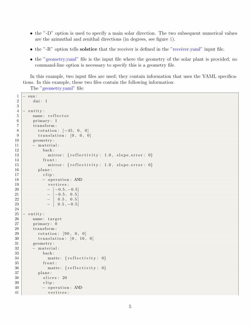
In this example, two input files are used; they contain information that uses the YAML specifica-tions. In this example, these two files contain the following information:

The ”geometry.yaml” file:

1 − sun :2 dni : 134 − en t i t y :5 name : r e f l e c t o r6 primary : 17 trans form :8 r o t a t i on : [−45 , 0 , 0 ]9 t r a n s l a t i o n : [ 0 , 0 , 0 ]

10 geometry :11 − mate r i a l :12 back :13 mirror : { r e f l e c t i v i t y : 1 . 0 , s l o p e e r r o r : 0}14 f r on t :15 mirror : { r e f l e c t i v i t y : 1 . 0 , s l o p e e r r o r : 0}16 plane :17 c l i p :18 − opera t ion : AND19 v e r t i c e s :20 − [−0.5 ,−0.5 ]21 − [−0.5 , 0 . 5 ]22 − [ 0 . 5 , 0 . 5 ]23 − [ 0 . 5 , −0 .5 ]2425 − en t i t y :26 name : t a r g e t27 primary : 028 trans form :29 r o t a t i on : [ 9 0 , 0 , 0 ]30 t r a n s l a t i o n : [ 0 , 10 , 0 ]31 geometry :32 − mate r i a l :33 back :34 matte : { r e f l e c t i v i t y : 0}35 f r on t :36 matte : { r e f l e c t i v i t y : 0}37 plane :38 s l i c e s : 2039 c l i p :40 − opera t ion : AND41 v e r t i c e s :

5

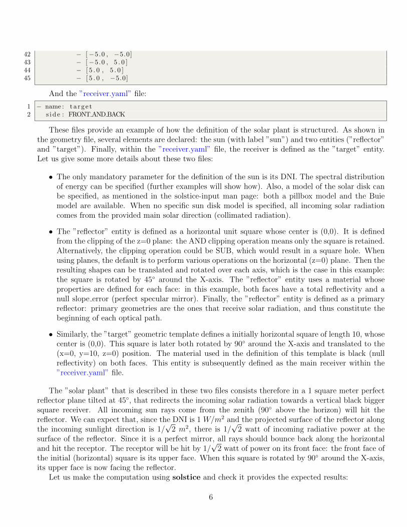
42 − [−5.0 , −5.0]43 − [−5.0 , 5 . 0 ]44 − [ 5 . 0 , 5 . 0 ]45 − [ 5 . 0 , −5.0]

And the ”receiver.yaml” file:

1 − name : t a r g e t2 s i d e : FRONTANDBACK

These files provide an example of how the definition of the solar plant is structured. As shown inthe geometry file, several elements are declared: the sun (with label ”sun”) and two entities (”reflector”and ”target”). Finally, within the ”receiver.yaml” file, the receiver is defined as the ”target” entity.Let us give some more details about these two files:

• The only mandatory parameter for the definition of the sun is its DNI. The spectral distributionof energy can be specified (further examples will show how). Also, a model of the solar disk canbe specified, as mentioned in the solstice-input man page: both a pillbox model and the Buiemodel are available. When no specific sun disk model is specified, all incoming solar radiationcomes from the provided main solar direction (collimated radiation).

• The ”reflector” entity is defined as a horizontal unit square whose center is (0,0). It is definedfrom the clipping of the z=0 plane: the AND clipping operation means only the square is retained.Alternatively, the clipping operation could be SUB, which would result in a square hole. Whenusing planes, the default is to perform various operations on the horizontal (z=0) plane. Then theresulting shapes can be translated and rotated over each axis, which is the case in this example:the square is rotated by 45◦ around the X-axis. The ”reflector” entity uses a material whoseproperties are defined for each face: in this example, both faces have a total reflectivity and anull slope error (perfect specular mirror). Finally, the ”reflector” entity is defined as a primaryreflector: primary geometries are the ones that receive solar radiation, and thus constitute thebeginning of each optical path.

• Similarly, the ”target” geometric template defines a initially horizontal square of length 10, whosecenter is (0,0). This square is later both rotated by 90◦ around the X-axis and translated to the(x=0, y=10, z=0) position. The material used in the definition of this template is black (nullreflectivity) on both faces. This entity is subsequently defined as the main receiver within the”receiver.yaml” file.

The ”solar plant” that is described in these two files consists therefore in a 1 square meter perfectreflector plane tilted at 45◦, that redirects the incoming solar radiation towards a vertical black biggersquare receiver. All incoming sun rays come from the zenith (90◦ above the horizon) will hit thereflector. We can expect that, since the DNI is 1 W/m2 and the projected surface of the reflector alongthe incoming sunlight direction is 1/

√2 m2, there is 1/

√2 watt of incoming radiative power at the

surface of the reflector. Since it is a perfect mirror, all rays should bounce back along the horizontaland hit the receptor. The receptor will be hit by 1/

√2 watt of power on its front face: the front face of

the initial (horizontal) square is its upper face. When this square is rotated by 90◦ around the X-axis,its upper face is now facing the reflector.

Let us make the computation using solstice and check it provides the expected results:

6

1 s o l s t i c e −D 0 ,90 −R r e c e i v e r . yaml geometry . yaml

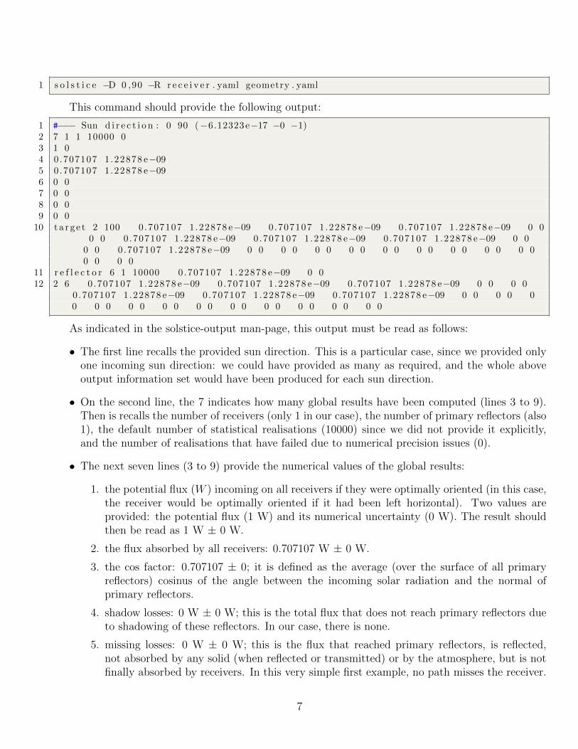
This command should provide the following output:

1 #−−− Sun d i r e c t i o n : 0 90 (−6.12323e−17 −0 −1)2 7 1 1 10000 03 1 04 0.707107 1.22878 e−095 0.707107 1.22878 e−096 0 07 0 08 0 09 0 0

10 ta r g e t 2 100 0.707107 1.22878 e−09 0.707107 1.22878 e−09 0.707107 1.22878 e−09 0 00 0 0.707107 1.22878 e−09 0.707107 1.22878 e−09 0.707107 1.22878 e−09 0 0

0 0 0.707107 1.22878 e−09 0 0 0 0 0 0 0 0 0 0 0 0 0 0 0 0 0 00 0 0 0

11 r e f l e c t o r 6 1 10000 0.707107 1.22878 e−09 0 012 2 6 0.707107 1.22878 e−09 0.707107 1.22878 e−09 0.707107 1.22878 e−09 0 0 0 0

0.707107 1.22878 e−09 0.707107 1.22878 e−09 0.707107 1.22878 e−09 0 0 0 0 00 0 0 0 0 0 0 0 0 0 0 0 0 0 0 0 0 0 0

As indicated in the solstice-output man-page, this output must be read as follows:

• The first line recalls the provided sun direction. This is a particular case, since we provided onlyone incoming sun direction: we could have provided as many as required, and the whole aboveoutput information set would have been produced for each sun direction.

• On the second line, the 7 indicates how many global results have been computed (lines 3 to 9).Then is recalls the number of receivers (only 1 in our case), the number of primary reflectors (also1), the default number of statistical realisations (10000) since we did not provide it explicitly,and the number of realisations that have failed due to numerical precision issues (0).

• The next seven lines (3 to 9) provide the numerical values of the global results:

1. the potential flux (W ) incoming on all receivers if they were optimally oriented (in this case,the receiver would be optimally oriented if it had been left horizontal). Two values areprovided: the potential flux (1 W) and its numerical uncertainty (0 W). The result shouldthen be read as 1 W ± 0 W.

2. the flux absorbed by all receivers: 0.707107 W ± 0 W.

3. the cos factor: 0.707107 ± 0; it is defined as the average (over the surface of all primaryreflectors) cosinus of the angle between the incoming solar radiation and the normal ofprimary reflectors.

4. shadow losses: 0 W ± 0 W; this is the total flux that does not reach primary reflectors dueto shadowing of these reflectors. In our case, there is none.

5. missing losses: 0 W ± 0 W; this is the flux that reached primary reflectors, is reflected,not absorbed by any solid (when reflected or transmitted) or by the atmosphere, but is notfinally absorbed by receivers. In this very simple first example, no path misses the receiver.

7

6. reflectivity losses: 0 W ± 0 W; this is the flux that has been absorbed by elements otherthat receivers (both solid surfaces and solid volumes such as semi-transparent materials).

7. absorptivity losses: 0 W ± 0 W; this is the flux that is absorbed by the atmosphere on thepath from a primary reflector to a receiver. Since we did not provide any information aboutatmospheric absorptivity, this value is null.

• Then one line of results is provided for each receiver (in this case, only one: line number 10).It provides the name of the receiver, its ID, its area in square meters, then 11x2 sets of results(result and its numerical uncertainty) for each side of the receiver (front and back). These 11 setsof results, for each side, are the following:

1. incoming flux over the receiver’s side

2. incoming flux over the receiver’s side if no absorption occurs in materials

3. incoming flux over the receiver’s side if no extinction occurs in the atmosphere

4. flux removed because of absorption in materials

5. flux removed because of extinction in the atmosphere

6. the flux that was absorbed by the receiver’s side

7. the flux that would be absorbed by the receiver’s side if no absorption occurs in materials

8. the flux that would be absorbed by the receiver’s side if no extinction occurs in the atmo-sphere

9. flux that has not been absorbed by the receiver’s side because of absorption by materials

10. flux that has not been absorbed by the receiver’s side because of extinction by the atmosphere

11. global efficiency: the fraction of the potential flux that was absorbed by the receiver’s side

In this case, these results are null (0 ± 0 watts) for the back side since radiation is absorbedonce it reaches the front side: as expected, a total of 0.707107 watt reached the front side of thereceiver, and all of it was absorbed because of the perfectly absorbing receiver, and nothing waslost because of absorption by imperfect reflectors, semi-transparent materials or the atmosphere.

• One line is then provided for each primary entity (one in our case: line number 11); it providesthe name of the primary reflector, its ID, its area in square meters, the number of statisticalrealisations that have been sampled on this reflector, and two sets of results for this primaryreflector:

1. the cos-factor of the reflector (0.707107 ± 0): average, over the surface of the reflector, ofthe cosinus of the angle between the direction of incoming radiation and the local normal tothe surface.

2. shadow losses of the reflector (0 ± 0): flux that did not reach the reflector because of primaryreflectors shadowing.

• Finally, one line is provided for each (receiver / primary reflector) couple. In our case, since thereare only one receiver and one primary reflector, there is only one such line (line 12). It providesthe ID of the receiver, the ID of the primary reflector, and 10 sets of results per receiver’s side(front / back):

8

1. incoming flux over the receiver’s side, coming from the reflector

2. incoming flux over the receiver’s side if no absorption occurs in materials, coming from thereflector

3. incoming flux over the receiver’s side if no extinction occurs in the atmosphere, coming fromthe reflector

4. flux removed because of absorption in materials, coming from the reflector

5. flux removed because of extinction in the atmosphere, coming from the reflector

6. the flux that was absorbed by the receiver’s side, coming from the reflector

7. the flux that would be absorbed by the receiver’s side if no absorption occurs in materials,coming from the reflector

8. the flux that would be absorbed by the receiver’s side if no extinction occurs in the atmo-sphere, coming from the reflector

9. flux that has not been absorbed by the receiver’s side because of absorption by materials,coming from the reflector

10. flux that has not been absorbed by the receiver’s side because of extinction by the atmo-sphere, coming from the reflector

In this case, only front results are non-null: as expected, all the reflected power (0.707107 watt)effectively reached the front side of the receiver, and all of it was absorbed. Nothing was absorbedby solid surfaces or semi-transparent materials, and nothing was absorbed by the atmosphere.

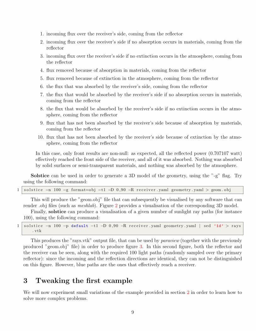
Solstice can be used in order to generate a 3D model of the geometry, using the ”-g” flag. Tryusing the following command:

1 s o l s t i c e −n 100 −g format=obj −t1 −D 0 ,90 −R r e c e i v e r . yaml geometry . yaml > geom . obj

This will produce the ”geom.obj” file that can subsequently be visualised by any software that canrender .obj files (such as meshlab). Figure 2 provides a visualisation of the corresponding 3D model.

Finally, solstice can produce a visualisation of a given number of sunlight ray paths (for instance100), using the following command:

1 s o l s t i c e −n 100 −p default −t1 −D 0 ,90 −R r e c e i v e r . yaml geometry . yaml | sed ’1d’ > rays. vtk

This produces the ”rays.vtk” output file, that can be used by paraview (together with the previouslyproduced ”geom.obj” file) in order to produce figure 3. In this second figure, both the reflector andthe receiver can be seen, along with the required 100 light paths (randomly sampled over the primaryreflector): since the incoming and the reflection directions are identical, they can not be distinguishedon this figure. However, blue paths are the ones that effectively reach a receiver.

3 Tweaking the first example

We will now experiment small variations of the example provided in section 2 in order to learn how tosolve more complex problems.

9

Figure 1: Definition of the zenithal and azimuthal angles

Figure 2: 3D model of the geometry used in the first example

10

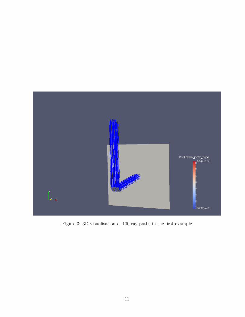
Figure 3: 3D visualisation of 100 ray paths in the first example

11

3.1 Solar disk models

The default model of the solar disk is that there is no solar disk: all incoming sunlight comes from thespecified sun direction. You can alternatively use two different solar disk models: the pillbox modeland the Buie model.

Try replacing the ”sun” section in the ”geometry.yaml” file by the following lines:

1 − sun : &sun2 dni : 13 p i l l b o x :4 h a l f a n g l e : 0 .535 spectrum : [{ wavelength : 1 , data : 1} ]

In this example, we tell solstice to use the pillbox model with an solar disk half-angle of 0.53◦: thesolar disk is now considered as a surface located at the end of a cone of 0.53◦ half-angle, with a uniformflux. The ”spectrum” attribute is optional, it could be removed in this example. Section 4 will describehow to use more complex spectra.

Then run the solstice computation again, with the same main solar direction:

1 s o l s t i c e −D 0 ,90 −R r e c e i v e r . yaml geometry . yaml

Produces:

1 #−−− Sun d i r e c t i o n : 0 90 (−6.12323e−17 −0 −1)2 7 1 1 10000 03 1 04 0.707075 3.27624 e−055 0.707107 1.22878 e−096 0 07 0 08 0 09 0 0

10 ta r g e t 2 100 0.707075 3.27624 e−05 0.707075 3.27624 e−05 0.707075 3.27624 e−05 0 00 0 0.707075 3.27624 e−05 0.707075 3.27624 e−05 0.707075 3.27624 e−05 0 0

0 0 0.707075 3.27624 e−05 0 0 0 0 0 0 0 0 0 0 0 0 0 0 0 0 0 00 0 0 0

11 r e f l e c t o r 6 1 10000 0.707107 1.22878 e−09 0 012 2 6 0.707075 3.27624 e−05 0.707075 3.27624 e−05 0.707075 3.27624 e−05 0 0 0 0

0.707075 3.27624 e−05 0.707075 3.27624 e−05 0.707075 3.27624 e−05 0 0 0 0 00 0 0 0 0 0 0 0 0 0 0 0 0 0 0 0 0 0 0

The main difference with the first set of results is that the computed power (incoming on thereflector, absorbed by the front face of the receiver) is computed with a non-null standard deviation.The direction of incoming solar radiation is now sampled within a small solid angle centered on themain solar direction.

We can also use the Buie model (presented in [1]). For instance, try replacing the ”sun” section inthe ”geometry.yaml” file by the following lines:

1 − sun : &sun2 dni : 13 buie :4 c s r : 0 . 15 spectrum : [{ wavelength : 1 , data : 1} ]

12

We have now specified the use of the Buie model, using a circumsolar ratio of 0.1; the distributionof solar flux varies with the position of emission along the solar disk, and a circumsolar ring due toatmospheric scattering is also taken into consideration. The output of solstice in this case is thefollowing:

1 #−−− Sun d i r e c t i o n : 0 90 (−6.12323e−17 −0 −1)2 7 1 1 10000 03 1 04 0.707053 3.14633 e−055 0.707107 1.22878 e−096 0 07 0 08 0 09 0 0

10 ta r g e t 2 100 0.707053 3.14633 e−05 0.707053 3.14633 e−05 0.707053 3.14633 e−05 0 00 0 0.707053 3.14633 e−05 0.707053 3.14633 e−05 0.707053 3.14633 e−05 0 0

0 0 0.707053 3.14633 e−05 0 0 0 0 0 0 0 0 0 0 0 0 0 0 0 0 0 00 0 0 0

11 r e f l e c t o r 6 1 10000 0.707107 1.22878 e−09 0 012 2 6 0.707053 3.14633 e−05 0.707053 3.14633 e−05 0.707053 3.14633 e−05 0 0 0 0

0.707053 3.14633 e−05 0.707053 3.14633 e−05 0.707053 3.14633 e−05 0 0 0 0 00 0 0 0 0 0 0 0 0 0 0 0 0 0 0 0 0 0 0

Once again, the dispersion of incoming sunlight directions translates only in a modification of thecos-factor and the total power that is absorbed by the receiver.

3.2 Surface properties of materials

In the first example, the definition of the material was embedded in the definition of the reflector. Is ispossible to define surface properties independently of entities. For instance, let us create a ”material”section in the ”geometry.yaml” file, prior to the definition of entities:

1 − mate r i a l : &custom2 mirror : { r e f l e c t i v i t y : 0 . 75 , s l o p e e r r o r : 0 }

The primary reflector must also be modified in order to use the ”custom” material:

1 − en t i t y :2 name : r e f l e c t o r3 primary : 14 trans form :5 r o t a t i on : [−45 , 0 , 0 ]6 t r a n s l a t i o n : [ 0 , 0 , 0 ]7 geometry :8 − mate r i a l : ∗custom9 plane :

10 c l i p :11 − opera t ion : AND12 v e r t i c e s :13 − [−0.5 ,−0.5 ]14 − [−0.5 , 0 . 5 ]15 − [ 0 . 5 , 0 . 5 ]16 − [ 0 . 5 , −0 .5 ]

13

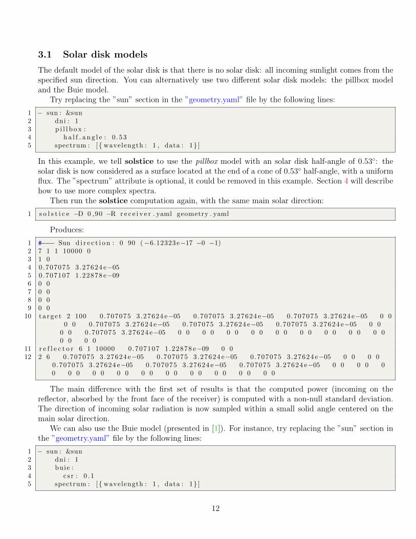
Figure 4: 3D visualisation of 100 ray paths in the example of a custom material with reflectivity=0.75and slope error=0.5

14

This mechanism provides the possibility to define the surface properties of as many materials asrequired, and to easily switch materials within the definition of the various entities.

The output of the solstice computation is now:

1 #−−− Sun d i r e c t i o n : 0 90 (−6.12323e−17 −0 −1)2 7 1 1 10000 03 1 04 0.53033 2.11523 e−095 0.707107 1.22878 e−096 0 07 0 08 0.176777 3.07195 e−109 0 0

10 ta r g e t 2 100 0.53033 2.11523 e−09 0.707107 1.22878 e−09 0.53033 2.11523 e−090.176777 3.08323 e−10 0 0 0.53033 2.11523 e−09 0.707107 1.22878 e−09 0.530332.11523 e−09 0.176777 3.08323 e−10 0 0 0.53033 2.11523 e−09 0 0 0 0 0 00 0 0 0 0 0 0 0 0 0 0 0 0 0 0 0

11 r e f l e c t o r 6 1 10000 0.707107 1.22878 e−09 0 012 2 6 0.53033 2.11523 e−09 0.707107 1.22878 e−09 0.53033 2.11523 e−09 0.176777

3.08323 e−10 0 0 0.53033 2.11523 e−09 0.707107 1.22878 e−09 0.53033 2.11523 e−09 0.176777 3.08323 e−10 0 0 0 0 0 0 0 0 0 0 0 0 0 0 0 0 0 00 0 0 0

Using a reflectivity of 0.75 instead of 1 has no consequence of the cos-factor, but the power that isabsorbed by the receiver is now 0.53033±0 watts. We can also see that 0.176777±0 watts have beenabsorbed by the reflector due to its partial reflectivity (within the global results, in the results line forthe receiver and the results line for the receiver/reflector couple).

We can also modify the value of the ”slope error” parameter in the properties of our ”custom”material; let us give it a non-null value:

1 − mate r i a l : &custom2 mirror : { r e f l e c t i v i t y : 0 . 75 , s l o p e e r r o r : 0 . 5 }

This ”slope error” parameter controls the reflection BRDF. We can see a clear effect on computationresults:

1 #−−− Sun d i r e c t i o n : 0 90 (−6.12323e−17 −0 −1)2 7 1 1 10000 03 1 04 0.096772 0.002048195 0.707107 1.22878 e−096 0 07 0.399882 0.001969138 0.210453 0.0005771289 0 0

10 ta r g e t 2 100 0.096772 0.00204819 0.129047 0.00273124 0.096772 0.002048190.032275 0.00068322 0 0 0.096772 0.00204819 0.129047 0.00273124 0.0967720.00204819 0.032275 0.00068322 0 0 0.096772 0.00204819 0 0 0 0 0 0 00 0 0 0 0 0 0 0 0 0 0 0 0 0 0

11 r e f l e c t o r 6 1 10000 0.707107 1.22878 e−09 0 012 2 6 0.096772 0.00204819 0.129047 0.00273124 0.096772 0.00204819 0.032275

0.00068322 0 0 0.096772 0.00204819 0.129047 0.00273124 0.096772 0.002048190.032275 0.00068322 0 0 0 0 0 0 0 0 0 0 0 0 0 0 0 0 0 0 0 00 0

15

The power that reaches the receiver’s back face is now significantly lower than the initial 0.707107watts, and now the flux lost to the environment (missing-loss) is non-null. Also, the additional flux thatcould have been absorbed by the receiver if the mirror was a perfect reflector is 3.25446e-2 ± 6.86322e-4watts. As can be seen in figure 4, reflection directions are scattered over the upper hemisphere, andsome rays are not reflected in the direction of the receiver (turquoise rays).

3.3 Rotating and translating geometric elements

As can be seen in the ”geometry.yaml” file, a ”transform” section can be added to the definition ofany given entity in order to apply a rotation of an arbitrary angle around each axis, and also to applya arbitrary translation along each axis. Positioning geometries in space is pretty straightforward fromthe provided example.

3.4 Geometric shapes

As mentioned in the solstice-input man page, the following geometric shapes can be defined in solstice:cuboids, cylinders, spheres, hemispheres, planes, paraboloids, hyperboloids, parabolic cylinders. Thereis also the possibility to include geometries that are defined using the STL format. Furthermore,clipping operations can be performed over parametric shapes (hemispheres, paraboloids, hyperboloids,parabolic cylinders and planes): this was the case throughout all previous examples, when defining thetwo squares from a original plane.

The user should refer to the man pages that provide extensive documentation on the way theseshapes can be defined. We will use various shapes in the following examples.

3.5 Pivots

Pivots provide the possibility to automatically rotate a given geometry in order to reflect incomingsunlight toward a given position. In solstice, two types of pivots are defined: the x pivot and thezx pivot. A example showing how to use both types will be provided.

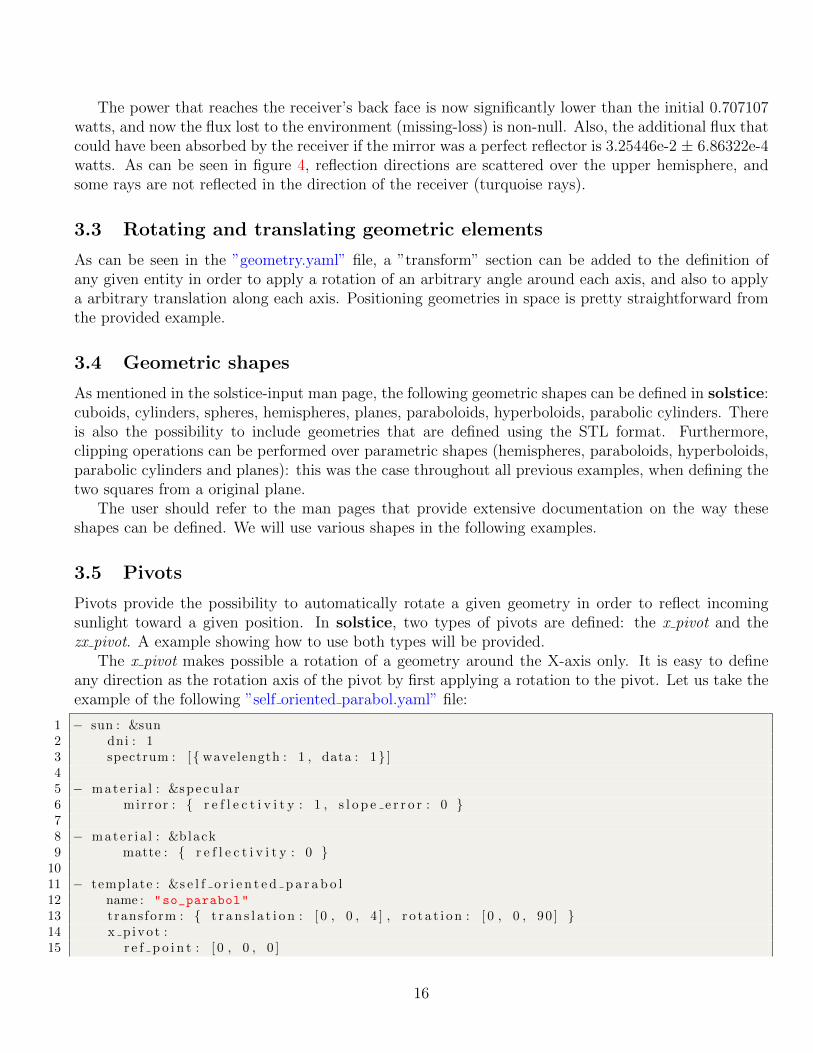
The x pivot makes possible a rotation of a geometry around the X-axis only. It is easy to defineany direction as the rotation axis of the pivot by first applying a rotation to the pivot. Let us take theexample of the following ”self oriented parabol.yaml” file:

1 − sun : &sun2 dni : 13 spectrum : [{ wavelength : 1 , data : 1} ]45 − mate r i a l : &specu l a r6 mirror : { r e f l e c t i v i t y : 1 , s l o p e e r r o r : 0 }78 − mate r i a l : &black9 matte : { r e f l e c t i v i t y : 0 }

1011 − template : &s e l f o r i e n t e d p a r a b o l12 name : "so_parabol"

13 trans form : { t r a n s l a t i o n : [ 0 , 0 , 4 ] , r o t a t i on : [ 0 , 0 , 90 ] }14 x p ivo t :15 r e f p o i n t : [ 0 , 0 , 0 ]

16

16 ta r g e t : { sun : ∗ sun }17 ch i l d r en :18 − name : "parabol"

19 primary : 120 geometry :21 − mate r i a l : ∗ sp e cu l a r22 parabol :23 f o c a l : 424 c l i p :25 − opera t ion : AND26 v e r t i c e s : [ [ −5 .0 , −5.0 ] , [−5.0 , 5 . 0 ] ,27 [ 5 . 0 , 5 . 0 ] , [ 5 . 0 , −5 .0 ] ]28 − name : "small_square"

29 trans form : { t r a n s l a t i o n : [ 0 , 0 , 4 ] }30 primary : 031 geometry :32 − mate r i a l : ∗black33 plane :34 c l i p :35 − opera t ion : AND36 v e r t i c e s : [ [ −0 .50 , −0.50] , [−0.50 , 0 . 5 0 ] ,37 [ 0 . 5 0 , 0 . 5 0 ] , [ 0 . 5 0 , −0 .50 ] ]3839 − en t i t y :40 name : "reflector"

41 trans form : { r o t a t i on : [ 0 , 0 , 0 ] , t r a n s l a t i o n : [ 0 , 0 , 0 ] }42 ch i l d r en : [ ∗ s e l f o r i e n t e d p a r a b o l ]

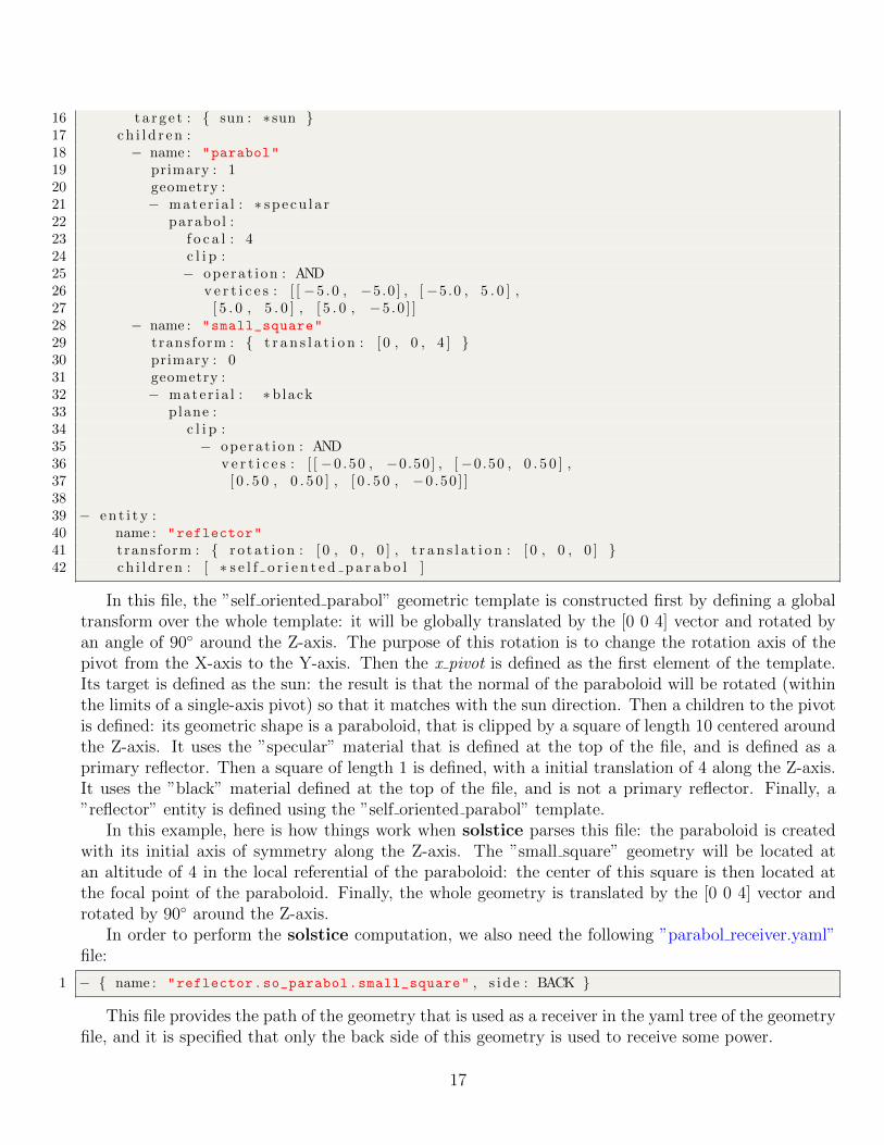
In this file, the ”self oriented parabol” geometric template is constructed first by defining a globaltransform over the whole template: it will be globally translated by the [0 0 4] vector and rotated byan angle of 90◦ around the Z-axis. The purpose of this rotation is to change the rotation axis of thepivot from the X-axis to the Y-axis. Then the x pivot is defined as the first element of the template.Its target is defined as the sun: the result is that the normal of the paraboloid will be rotated (withinthe limits of a single-axis pivot) so that it matches with the sun direction. Then a children to the pivotis defined: its geometric shape is a paraboloid, that is clipped by a square of length 10 centered aroundthe Z-axis. It uses the ”specular” material that is defined at the top of the file, and is defined as aprimary reflector. Then a square of length 1 is defined, with a initial translation of 4 along the Z-axis.It uses the ”black” material defined at the top of the file, and is not a primary reflector. Finally, a”reflector” entity is defined using the ”self oriented parabol” template.

In this example, here is how things work when solstice parses this file: the paraboloid is createdwith its initial axis of symmetry along the Z-axis. The ”small square” geometry will be located atan altitude of 4 in the local referential of the paraboloid: the center of this square is then located atthe focal point of the paraboloid. Finally, the whole geometry is translated by the [0 0 4] vector androtated by 90◦ around the Z-axis.

In order to perform the solstice computation, we also need the following ”parabol receiver.yaml”file:

1 − { name : "reflector.so_parabol.small_square" , s i d e : BACK }

This file provides the path of the geometry that is used as a receiver in the yaml tree of the geometryfile, and it is specified that only the back side of this geometry is used to receive some power.

17

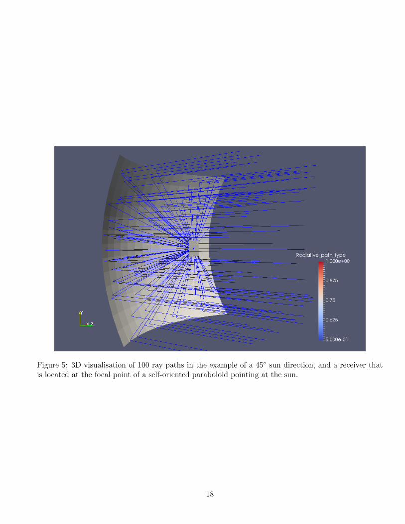
Figure 5: 3D visualisation of 100 ray paths in the example of a 45◦ sun direction, and a receiver thatis located at the focal point of a self-oriented paraboloid pointing at the sun.

18

We can finally perform the computation:

1 s o l s t i c e −D 0 ,45 −R pa r abo l r e c e i v e r . yaml s e l f o r i e n t e d p a r a b o l . yaml

with the following result:

1 #−−− Sun d i r e c t i o n : 0 45 (−0.707107 −0 −0.707107)2 7 1 1 10000 03 111 .97 04 98 .91 0.1038335 0.893096 06 1 .09 0.1038337 0 08 0 09 0 0

10 r e f l e c t o r . s o parabo l . sma l l squa r e 6 1 −1 −1 −1 −1 −1 −1 −1 −1 −1 −1 −1 −1−1 −1 −1 −1 −1 −1 −1 −1 −1 −1 98 .91 0.103833 98 .91 0.103833 98 .91

0.103833 0 0 0 0 98 .91 0.103833 98 .91 0.103833 98 .91 0.103833 0 0 0 00.883361 0.000927324

11 r e f l e c t o r . s o parabo l . parabol 2 111 .97 10000 0.893096 0 1 .09 0.10383312 6 2 −1 −1 −1 −1 −1 −1 −1 −1 −1 −1 −1 −1 −1 −1 −1 −1 −1 −1 −1 −1

98 .91 0.103833 98 .91 0.103833 98 .91 0.103833 0 0 0 0 98 .91 0.10383398 .91 0.103833 98 .91 0.103833 0 0 0 0

Over the 111.97±0 watts incoming on the surface of the paraboloid, only 98.81±0.108 watts arefocused on the receiver: this is partly due to a cos-factor different from 1 (the potential flux is 111.97watts because the DNI is 1 watt per square meter, and the surface of the paraboloid is 111.97 squaremeters; however, because of the curvature of the paraboloid, it intercepts only 100 watts: 111.97*cos-factor), and to the fact that 1.19±0.108 watts are lost because of the shadow that the receiver casts onthe paraboloid. No power is lost by the receiver and there are no reflectivity losses due to absorption.Figure 5 provides a visualisation of the scene.

The zx pivot makes possible a rotation around two perpendicular axis. In the following ”tworeflectors one receiver.yaml” file, two paraboloids are defined from the same ”self oriented parabol”geometric template (a paraboloid with a focal distance of 100 meters). These two reflectors are locatedat different spatial directions, and reflect radiation back to a common square receiver.

1 − sun : &sun2 dni : 13 spectrum : [{ wavelength : 1 , data : 1} ]4 # Po s s i b i l i t y to prov ide as many wavelength va lue s ( and correspond ing5 # s o l a r i r r a d i a n c e at ground l e v e l ) as requ i red , in order to6 # take in to account the s p e c t r a l dependence to the s o l a r emis s ion7 # and atmosphere absorpt ion .89 # De f i n i t i o n o f mat e r i a l s

10 − mate r i a l : &lambert ian11 f r on t :12 matte : { r e f l e c t i v i t y : 1 }13 back :14 matte : { r e f l e c t i v i t y : 1 }1516 − mate r i a l : &specu l a r17 mirror : { r e f l e c t i v i t y : 1 , s l o p e e r r o r : 0 }

19

1819 − mate r i a l : &black20 matte : { r e f l e c t i v i t y : 0 }2122 # De f i n i t i o n o f the ” sma l l squa r e ” geometry that w i l l be used23 # by the r e c e i v e r24 − geometry : &sma l l squa r e25 − mate r i a l : ∗black26 plane :27 c l i p :28 − opera t ion : AND29 v e r t i c e s :30 − [−0.50 , −0.50]31 − [−0.50 , 0 . 5 0 ]32 − [ 0 . 5 0 , 0 . 5 0 ]33 − [ 0 . 5 0 , −0.50]3435 # De f i n i t i o n o f the r e c e i v e r ’ s e n t i t y .36 − en t i t y :37 name : "square_receiver"

38 primary : 039 # se t ”primary” to 0 because t h i s e n t i t y should not the sampled40 # as a primary r e f l e c t o r41 trans form : { r o t a t i on : [ 0 , 90 , 0 ] , t r a n s l a t i o n : [ 100 , 0 , 10 ] }42 # The ” sma l l squa r e ” geometry i s c r ea ted as ho r i z on t a l . In order to43 # have i t v e r t i c a l , a r o t a t i on o f 90 degree s around the Y−ax i s44 # must be performed .45 # Also , a t r a n s l a t i o n i s app l i ed in order to po s i t i o n i t in space .46 anchors :47 − name : "anchor0"

48 po s i t i o n : [ 0 , 0 , 0 ]49 # An anchor i s de f ined , at a l o c a l p o s i t i o n ( in the r e f e r e n t i a l o f50 # the square )51 geometry : ∗ sma l l squa r e525354 # De f i n i t i o n o f a geometry template f o r primary r e f l e c t o r s ( parabol )55 − template : &s e l f o r i e n t e d p a r a b o l56 name : "so_parabol"

57 trans form : { t r a n s l a t i o n : [ 0 , 0 , 4 ] , r o t a t i on : [ 0 , 0 , 90 ] }58 # The 90−degree s r o t a t i on around the Z−ax i s i s r equ i r ed so that the59 # pivot r o t a t e s around the Y−ax i s and not the X−ax i s .60 zx p ivo t :61 r e f p o i n t : [ 0 , 0 , 0 ]62 t a r g e t : { anchor : s q u a r e r e c e i v e r . anchor0 }63 # the ta r g e t i s the anchor that was p r ev i ou s l y de f ined in64 # the r e c e i v e r ’ s e n t i t y ( the cente r o f the square )65 ch i l d r en :66 − name : "parabol"

67 trans form : { r o t a t i on : [−90 , 0 , 0 ] , t r a n s l a t i o n : [ 0 , 0 , 0 ] }68 # This −90−degree s r o t a t i on over the X−ax i s i s r equ i r ed because :69 # − the parabol i s generated ” ho r i z on t a l ” : i t s c e n t r a l ax i s i s the Z−ax i s70 # − the automatic o r i e n t a t i o n o f the parabol w i l l be performed so that71 # the Y−ax i s i s the l o c a l normal o f the spe cu l a r r e f l e x i o n @ r e f p o i n t

20

72 # − a 90−degree s r o t a t i on around the Z−ax i s i s app l i ed73 # => in order to make the X−ax i s the l o c a l normal o f spe cu l a r r e f l e x i o n ,74 # the parabol must be ro ta ted by −90−degree s around X and then75 # by 90−degree s around Z .76 primary : 1 # primary=1 −> sampled f o r i n t e g r a t i o n77 geometry :78 − mate r i a l : ∗ sp e cu l a r79 parabol :80 f o c a l : 10081 c l i p :82 − opera t ion : AND83 v e r t i c e s : [ [ −5 .0 , −5.0 ] , [−5.0 , 5 . 0 ] , [ 5 . 0 , 5 . 0 ] , [ 5 . 0 , −5 .0 ] ]8485 # Two i d e n t i c a l parabo l s are p laced at two d i f f e r e n t l o c a t i o n s .86 # Automatic o r i e n t a t i o n o f the parabo l s so that a spe cu l a r87 # r e f l e x i o n o f the sun ’ s main d i r e c t i o n at the cente r o f the parabol88 # i s d i r e c t ed to the cente r o f the r e c e i v e r .89 − en t i t y :90 name : "reflector1"

91 trans form : { r o t a t i on : [ 0 , 0 , 0 ] , t r a n s l a t i o n : [ 0 , 0 , 0 ] }92 ch i l d r en : [ ∗ s e l f o r i e n t e d p a r a b o l ]9394 − en t i t y :95 name : "reflector2"

96 trans form : { r o t a t i on : [ 0 , 0 , 0 ] , t r a n s l a t i o n : [ 1 0 , 43 . 6 , 0 ] }97 ch i l d r en : [ ∗ s e l f o r i e n t e d p a r a b o l ]

In this example, the same geometric template is used to define both primary reflectors: this”self oriented parabol” uses a zx pivot in order to position each reflector so that radiation is sentback to the center of the receiver (using the notion of anchor).

The following ”common receiver.yaml” file is used to define the receiver:

1 − { name : "square_receiver" , s i d e : BACK }

We can finally run solstice:

1 s o l s t i c e −n 100000 −t1 −D 0 ,45 −R common receiver . yaml tw o r e f l e c t o r s o n e r e c e i v e r . yaml

with the following result:

1 #−−− Sun d i r e c t i o n : 0 45 (−0.707107 −0 −0.707107)2 7 1 2 100000 03 200 .04 04 176.935 0.1210855 0.925156 3.46816 e−056 0 07 8.13302 0.1190258 0 09 0 0

10 s qu a r e r e c e i v e r 2 1 −1 −1 −1 −1 −1 −1 −1 −1 −1 −1 −1 −1 −1 −1 −1 −1−1 −1 −1 −1 −1 −1 176.935 0.121085 176.935 0.121085 176.935 0.121085 00 0 0 176.935 0.121085 176.935 0.121085 176.935 0.121085 0 0 0 00.884499 0.000605303

11 r e f l e c t o r 2 . s o parabo l . parabol 8 100 .02 50222 0.915688 2.58316 e−05 0 012 r e f l e c t o r 1 . s o parabo l . parabol 6 100 .02 49778 0.934708 2.29155 e−05 0 0

21

13 2 8 −1 −1 −1 −1 −1 −1 −1 −1 −1 −1 −1 −1 −1 −1 −1 −1 −1 −1 −1 −183.8607 0.288723 83.8607 0.288723 83.8607 0.288723 0 0 0 0 83.86070.288723 83.8607 0.288723 83.8607 0.288723 0 0 0 0

14 2 6 −1 −1 −1 −1 −1 −1 −1 −1 −1 −1 −1 −1 −1 −1 −1 −1 −1 −1 −1 −193.0744 0.295646 93.0744 0.295646 93.0744 0.295646 0 0 0 0 93.07440.295646 93.0744 0.295646 93.0744 0.295646 0 0 0 0

Within the solstice command, the ”-n 100000” option is used to explicitly specify the code willhave to sample 105 statistical realisations (in order to achieve a higher numerical accuracy), and the”-t1” option tells the code to run the computation on 1 thread, even if by default it uses all availablethreads.

Similarly to the previous example, only a fraction of the radiation available on the reflectors isfocused on the receiver. This is partly due to a cos-factor different from 1. And even if there isno shadow over the reflectors, there is some power that is reflected but does not reach the receptor(8.13±0.12 watts) because even if incoming sunlight is collimated, the sun direction does not matchthe normal of the second paraboloid (”reflector2”).

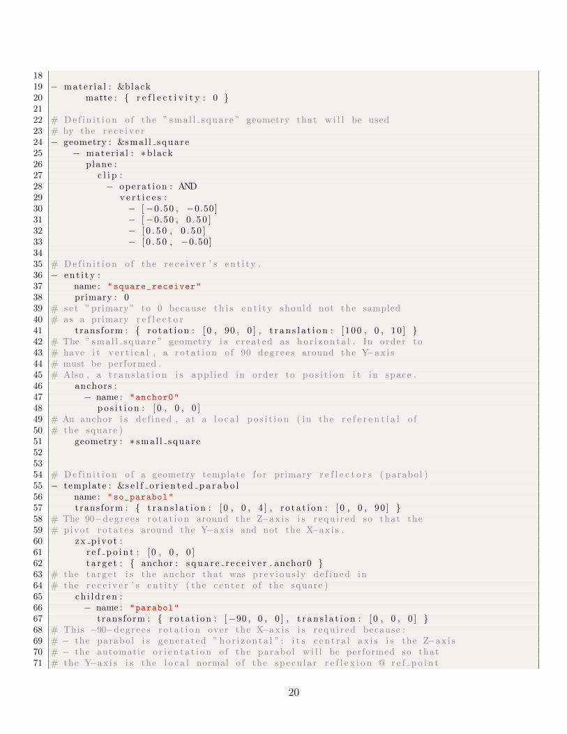
Figure 6 provides a visualisation of the scene. We can see some turquoise paths that originate fromthe ”reflector2” paraboloid.

4 A more complex example

The example provided in this section is not intended at describing a realistic solar plant. Instead, itspurpose is to use as many concepts as possible in the definition of the geometry.

In the following ”multiple reflectors.yaml” file, three primary reflectors made from parabolic sec-tions, with different focal distances, focus incoming sunlight at a common point. This point happensto be the upper focal point of a secondary reflector, in the shape of a hyperboloid (beam-down). Thena receptor is located at the second focal position of the hyperboloid. But in this last part of the opticalpath, a glass box has been placed. Figures 7 and 8 show the geometric configuration and optical pathswhen the box is set to use two different refractive materials.

1 # De f i n i t i o n o f spec t ra :2 # spectrum of incoming sun l i gn t3 − spectrum : &so la r spec t rum4 − {wavelength : 0 . 30 , data : 1 .0}5 − {wavelength : 0 . 40 , data : 2 .0}6 − {wavelength : 0 . 50 , data : 0 .5}7 − {wavelength : 0 . 60 , data : 3 .5}8 − {wavelength : 0 . 70 , data : 1 .5}9 − {wavelength : 0 . 80 , data : 0 .8}

10 # spectrum of a i r absorpt ion c o e f f i c i e n t11 − spectrum : &a i r kab s12 − {wavelength : 0 . 30 , data : 1 . 0 e−4}13 − {wavelength : 0 . 40 , data : 1 . 0 e−5}14 − {wavelength : 0 . 50 , data : 2 . 0 e−5}15 − {wavelength : 0 . 60 , data : 2 . 0 e−4}16 − {wavelength : 0 . 70 , data : 3 . 0 e−5}17 − {wavelength : 0 . 80 , data : 1 . 0 e−4}18 # spectrum of g l a s s absorpt ion c o e f f i c i e n t19 − spectrum : &g l a s s kab s

22

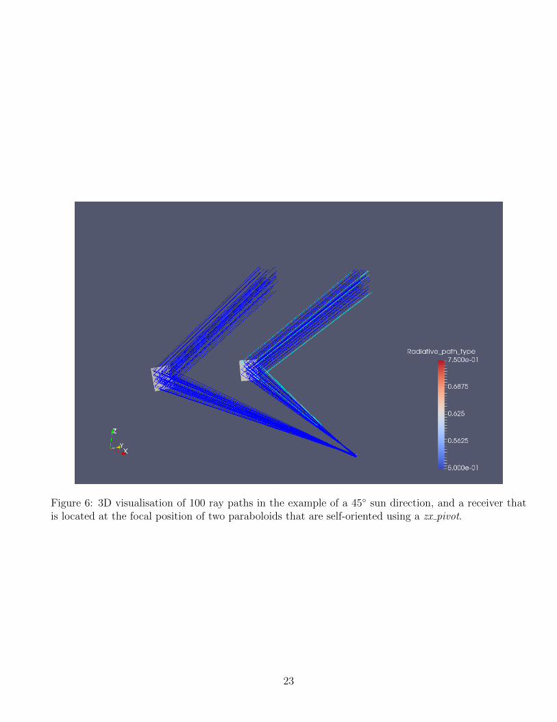
Figure 6: 3D visualisation of 100 ray paths in the example of a 45◦ sun direction, and a receiver thatis located at the focal position of two paraboloids that are self-oriented using a zx pivot.

23

20 − {wavelength : 0 . 30 , data : 1 . 0 e−2}21 − {wavelength : 0 . 40 , data : 1 . 0 e−3}22 − {wavelength : 0 . 50 , data : 2 . 0 e−3}23 − {wavelength : 0 . 60 , data : 2 . 0 e−2}24 − {wavelength : 0 . 70 , data : 3 . 0 e−3}25 − {wavelength : 0 . 80 , data : 1 . 0 e−3}26 # spectrum of g l a s s r e f r a c t i v e index27 − spectrum : &g l a s s r e f i n d e x28 − {wavelength : 0 . 30 , data : 1 .40}29 − {wavelength : 0 . 40 , data : 1 .39}30 − {wavelength : 0 . 50 , data : 1 .37}31 − {wavelength : 0 . 60 , data : 1 .34}32 − {wavelength : 0 . 70 , data : 1 .30}33 − {wavelength : 0 . 80 , data : 1 .25}3435 − sun : &sun36 dni : 137 buie :38 c s r : 0 .0539 spectrum : ∗ so l a r spec t rum4041 # De f i n i t i o n o f media42 # medium : a i r43 − medium : &air medium44 r e f r a c t i v e i n d e x : 145 e x t i n c t i o n : ∗ a i r k ab s46 # medium : g l a s s47 − medium : &glass medium48 r e f r a c t i v e i n d e x : ∗ g l a s s r e f i n d e x49 ex t i n c t i o n : ∗ g l a s s kab s5051 # De f i n i t i o n o f mat e r i a l s52 # lambert ian r e f l e c t i o n53 − mate r i a l : &lambert ian54 f r on t :55 matte : { r e f l e c t i v i t y : 1 }56 back :57 matte : { r e f l e c t i v i t y : 1 }58 # specu l a r r e f l e x i o n59 − mate r i a l : &specu l a r60 mirror : { r e f l e c t i v i t y : 1 , s l o p e e r r o r : 0 }61 # blackbody ( no r e f l e x i o n )62 − mate r i a l : &black63 mirror : { r e f l e c t i v i t y : 0 , s l o p e e r r o r : 0 }64 # th in g l a s s : uses the ” t h i n d i e l e c t r i c ” mate r i a l65 − mate r i a l : &t h i n g l a s s66 t h i n d i e l e c t r i c :67 th i ckne s s : 0 .00168 medium i : ∗air medium69 medium t : ∗glass medium70 # g l a s s : uses the ” d i e l e c t r i c ” mate r i a l71 − mate r i a l : &g l a s s72 f r on t :73 d i e l e c t r i c :

24

74 medium i : ∗air medium75 medium t : ∗glass medium76 back :77 d i e l e c t r i c :78 medium i : ∗glass medium79 medium t : ∗air medium8081 # De f i n i t i o n o f the ” sma l l squa r e ” geometry that w i l l be used82 # by the r e c ep to r83 − geometry : &sma l l squa r e84 − mate r i a l : ∗black85 plane :86 c l i p :87 − opera t ion : AND88 v e r t i c e s :89 − [−0.50 , −0.50]90 − [−0.50 , 0 . 5 0 ]91 − [ 0 . 5 0 , 0 . 5 0 ]92 − [ 0 . 5 0 , −0.50]9394 # De f i n i t i o n o f the ” g l a s s box ” geometry that w i l l be used95 # by the g l a s s96 − geometry : &g l a s s box97 − mate r i a l : ∗ t h i n g l a s s98 # − mate r i a l : ∗ g l a s s99 cuboid :100 s i z e : [ 1 0 , 1 0 , 0 . 5 ]101 trans form : { t r a n s l a t i o n : [ 0 , 0 , 0 . 2 5 ] }102103 # De f i n i t i o n o f the r e c e i v e r ’ s e n t i t y .104 − en t i t y :105 name : "square_receiver"

106 primary : 0107 # se t ”primary” to 0 because t h i s e n t i t y should not the sampled as a primary r e f l e c t o r108 trans form : { r o t a t i on : [ 0 , 0 , 0 ] , t r a n s l a t i o n : [ 0 , 0 , −10] }109 # The ” sma l l squa r e ” geometry i s c r ea ted as ho r i z on t a l . In order to110 # have i t v e r t i c a l , a r o t a t i on o f 90 degree s around the Y−ax i s must be performed .111 # Also , a t r a n s l a t i o n i s app l i ed in order to po s i t i o n i t in space .112 anchors :113 − name : "anchor0"

114 po s i t i o n : [ 0 , 0 , 0 ]115 # An anchor i s de f ined , at a l o c a l p o s i t i o n ( in the r e f e r e n t i a l o f the square )116 geometry : ∗ sma l l squa r e117118 # De f i n i t i o n o f a g l a s s box119 − en t i t y :120 name : "glass_slide"

121 primary : 0122 trans form : { r o t a t i on : [ 0 , 0 , 0 ] , t r a n s l a t i o n : [ 0 , 0 , 0 ] }123 geometry : ∗ g l a s s box124125 # De f i n i t i o n o f the primary r e f l e c t o r s126 − en t i t y :127 name : "primary_reflector1"

25

128 primary : 1 # primary=1 −> sampled f o r i n t e g r a t i o n129 trans form : { r o t a t i on : [ 0 , 0 , 0 ] , t r a n s l a t i o n : [ 0 , 0 , −2.0] }130 geometry :131 − mate r i a l : ∗ sp e cu l a r132 parabol :133 f o c a l : 12134 c l i p :135 − opera t ion : AND136 c i r c l e :137 rad iu s : 10138 cente r : [ 0 , 0 ]139 − opera t ion : SUB140 c i r c l e :141 rad iu s : 5142 cente r : [ 0 , 0 ]143144 − en t i t y :145 name : "primary_reflector2"

146 primary : 1 # primary=1 −> sampled f o r i n t e g r a t i o n147 trans form : { r o t a t i on : [ 0 , 0 , 0 ] , t r a n s l a t i o n : [ 0 , 0 , −4] }148 geometry :149 − mate r i a l : ∗ sp e cu l a r150 parabol :151 f o c a l : 14152 c l i p :153 − opera t ion : AND154 c i r c l e :155 rad iu s : 15156 cente r : [ 0 , 0 ]157 − opera t ion : SUB158 c i r c l e :159 rad iu s : 10160 cente r : [ 0 , 0 ]161162163 − en t i t y :164 name : "primary_reflector3"

165 primary : 1 # primary=1 −> sampled f o r i n t e g r a t i o n166 trans form : { r o t a t i on : [ 0 , 0 , 0 ] , t r a n s l a t i o n : [ 0 , 0 , −6] }167 geometry :168 − mate r i a l : ∗ sp e cu l a r169 parabol :170 f o c a l : 16171 c l i p :172 − opera t ion : AND173 c i r c l e :174 rad iu s : 20175 cente r : [ 0 , 0 ]176 − opera t ion : SUB177 c i r c l e :178 rad iu s : 15179 cente r : [ 0 , 0 ]180181

26

182 # De f i n i t i o n o f the secondary r e f l e c t o r183 − en t i t y :184 name : "secondary_reflector"

185 primary : 0 # primary=0 −> NOT sampled f o r i n t e g r a t i o n186 trans form : { r o t a t i on : [ 0 , 0 , 0 ] , t r a n s l a t i o n : [ 0 , 0 , 6 ] }187 geometry :188 − mate r i a l : ∗ sp e cu l a r189 hyperbol :190 f o c a l s : &hyp e r b o l f o c a l s { r e a l : 16 . 0 , image : 4 }191 c l i p :192 − opera t ion : AND193 c i r c l e :194 rad iu s : 5195 cente r : [ 0 , 0 ]196197 # Atmospheric absorpt ion p r op e r t i e s198 − atmosphere :199 e x t i n c t i o n : ∗ a i r k ab s

The following ”horizontal receiver.yaml” file is used to define the receiver:

1 − { name : "square_receiver" , s i d e : FRONT }

The ”horizontal receiver.yaml” file illustrates the use of the following new concepts:

• Spectra: at the beginning of the file, 4 different spectra are defined in order to describe thespectral dependence of: the incoming sunlight (”solar spectrum”), the absorption coefficient of theatmosphere (”air kabs”), the absorption coefficient of the glass (”glass kabs”), and the refractionindex of the glass (”glass ref index”). These spectra have been defined from 0.3 to 0.8 micrometerswith a step of 0.1 micrometer, but any spectral discretisation can be used, with no limit on thenumber of wavelengths.

• Two media have been defined: air (”air medium”) and glass (”glass medium”). Each mediumneeds the definition of its refraction index and its absorption coefficient. These properties can bea constant, such as in the case of the refraction index of air, or a spectrum.

• Two new categories of material properties are introduced: ”thin dielectric” and ”dielectric” thatare used respectively in the ”thin glass” and ”glass” materials. In each case, the ”medium i” and”medium t” properties need to be set using the previously defined ”air medium” and ”glass medium”media: ”medium i” refers to the medium on the exterior of the material, while ”medium t” refersto the medium on the interior of the material. Since ”thin dielectric” is a surface property, wedo not need to distinguish between the front and back side properties, but we need to define thethickness of the material. However, ”dielectric” is a volume property. But since we will use itover a geometry that is defined by its surface (see the ”glass box” geometry), we need to providesome information about what ”medium i” and ”medium t” refers to, for each side of this surface.

• The ”cuboid” shape is used in order to define the ”glass box” geometric template. It is later usedto define the ”glass slide” geometric entity.

• The ”circle” shape is used in order to perform clipping operations over the three paraboloids andthe hyperboloid.

27

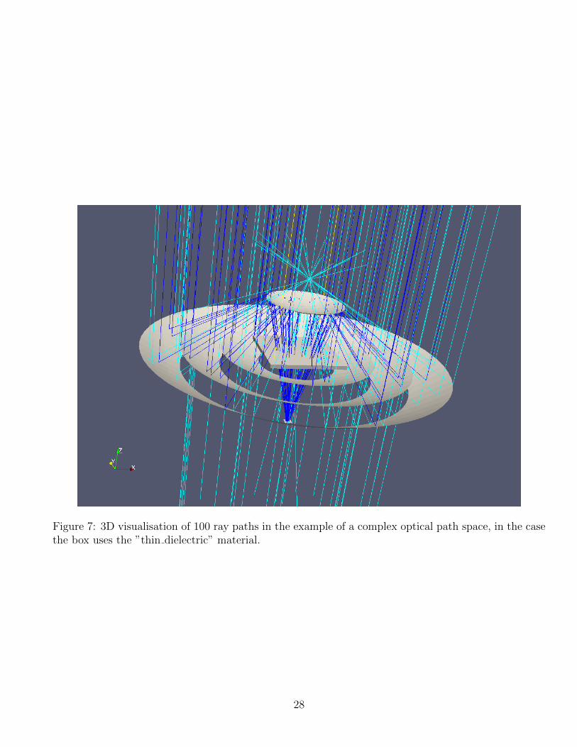
Figure 7: 3D visualisation of 100 ray paths in the example of a complex optical path space, in the casethe box uses the ”thin dielectric” material.

28

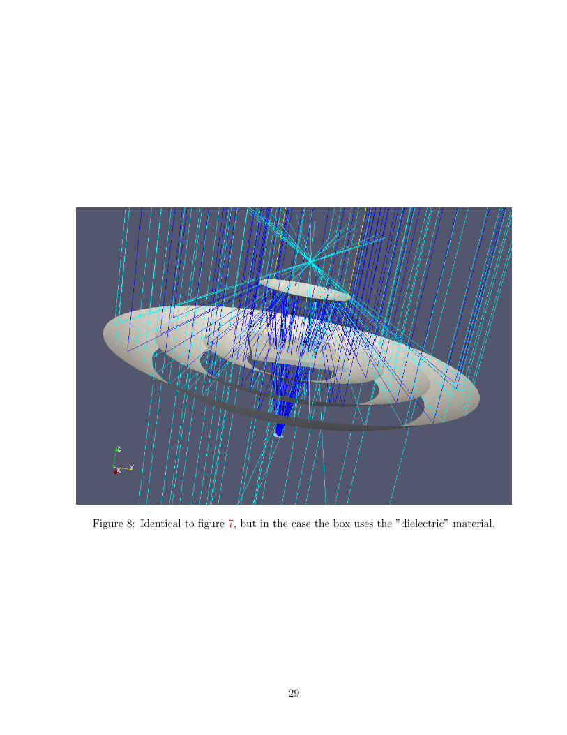
Figure 8: Identical to figure 7, but in the case the box uses the ”dielectric” material.

29

• Finally, the absorption optical properties of the atmosphere are set, using the ”air kabs” spectrumthat was defined at the beginning of the file.

Note that the ”glass box” template was defined using the ”thin glass” material (line 97). Whenrunning the solstice computation:

1 s o l s t i c e −v −D 0 ,90 −R ho r i z o n t a l r e c e i v e r . yaml mu l t i p l e r e f l e c t o r s . yaml

The output is the following:

1 #−−− Sun d i r e c t i o n : 0 90 (−6.12323e−17 −0 −1)2 7 1 3 10000 03 1304.77 04 566 .86 5 .86245 0.901466 06 22.1126 1 .59757 585.567 5.879178 0.011813 0.0001795919 1.64295 0.0203065

10 s qu a r e r e c e i v e r 10 1 566 .86 5 .8624 566 .87 5 .8625 568.312 5 .8774 0.01035910.000162878 1.45212 0.0204591 566 .86 5 .8624 566 .87 5 .8625 568.312 5 .87740.0103591 0.000162878 1.45212 0.0204591 0.434452 0.00449305 −1 −1 −1 −1−1 −1 −1 −1 −1 −1 −1 −1 −1 −1 −1 −1 −1 −1 −1 −1 −1 −1

11 p r ima r y r e f l e c t o r 2 2 430.566 3329 0.901466 0 0.23551 0.16651412 p r ima r y r e f l e c t o r 3 18 626.685 4642 0.901466 0 0.117683 0.11767713 p r ima r y r e f l e c t o r 1 22 247.518 2029 0.901466 2.16927 e−09 21.7595 1.5849214 10 2 250.228 4.80559 250.233 4.80567 250.875 4.81801 0.00428719 0.000109752

0.646888 0.0155304 250.228 4.80559 250.233 4.80567 250.875 4.818010.00428719 0.000109752 0.646888 0.0155304 −1 −1 −1 −1 −1 −1 −1 −1 −1 −1−1 −1 −1 −1 −1 −1 −1 −1 −1 −1

15 10 18 120.194 3.55664 120.196 3.55671 120.547 3.56706 0.00207403 7 .8854 e−050.352295 0.0126445 120.194 3.55664 120.196 3.55671 120.547 3.567060.00207403 7 .8854 e−05 0.352295 0.0126445 −1 −1 −1 −1 −1 −1 −1 −1 −1 −1−1 −1 −1 −1 −1 −1 −1 −1 −1 −1

16 10 22 196.437 4.38091 196.441 4 .381 196 .89 4 .39101 0.00399788 0.0001230050.452937 0.0123931 196.437 4.38091 196.441 4 .381 196 .89 4 .39101 0.003997880.000123005 0.452937 0.0123931 −1 −1 −1 −1 −1 −1 −1 −1 −1 −1 −1 −1−1 −1 −1 −1 −1 −1 −1 −1

We can see that from the 1304.77 watts that could potentially reach primary reflectors, only1304.77*0.901466=1176.21 watts are really intercepted by primary reflectors, and 560.165±5.8 wattsare finally absorbed by the receiver: 21.76±1.58 watts are lost because of shadowing, 592.65±5.9 wattsare lost because their optical paths do not end on the receiver, 1.17e-2±1.80e-4 watts are absorbed dur-ing surface reflections and by semi-transparent solids (the glass), and 1.63±2.0e-2 watts are lost becauseof atmospheric absorption. Figure 7 shows a representation of 100 optical paths in the geometry.

We can try to change the material of the glass box: let us comment line 97 and uncomment line98, thus defining the ”glass box” made of the ”glass” material (that uses the ”dielectric” materialproperty). The output of the computation is the following:

1 #−−− Sun d i r e c t i o n : 0 90 (−6.12323e−17 −0 −1)2 7 1 3 10000 03 1304.77 04 570.507 5.83915

30

5 0.901466 06 22.2294 1 .60167 578.202 5.868818 3.68103 0.144799 1.57284 0.0195712

10 s qu a r e r e c e i v e r 10 1 570.507 5 .83915 573.014 5.86468 571.926 5 .85361 2.506420.0385616 1.41933 0.0198379 570.507 5.83915 573.014 5.86468 571.926 5 .85361

2.50642 0.0385616 1.41933 0.0198379 0.437247 0.00447524 −1 −1 −1 −1 −1−1 −1 −1 −1 −1 −1 −1 −1 −1 −1 −1 −1 −1 −1 −1 −1 −1

11 p r ima r y r e f l e c t o r 2 2 430.566 3324 0.901466 0 0.23551 0.16651412 p r ima r y r e f l e c t o r 3 18 626.685 4661 0.901466 0 0.117683 0.11767713 p r ima r y r e f l e c t o r 1 22 247.518 2015 0.901466 2.12557 e−09 21.8762 1.5890514 10 2 259.355 4 .8553 260.456 4.87583 260.007 4.86745 1.10059 0.0275051

0.651655 0.0152761 259.355 4 .8553 260.456 4.87583 260.007 4.86745 1.100590.0275051 0.651655 0.0152761 −1 −1 −1 −1 −1 −1 −1 −1 −1 −1 −1 −1 −1−1 −1 −1 −1 −1 −1 −1

15 10 18 120.882 3.55773 121.386 3.57253 121.221 3.56768 0.504345 0.01947790.33895 0.0122011 120.882 3.55773 121.386 3 .57253 121.221 3.56768 0.5043450.0194779 0.33895 0.0122011 −1 −1 −1 −1 −1 −1 −1 −1 −1 −1 −1 −1 −1−1 −1 −1 −1 −1 −1 −1

16 10 22 190 .27 4 .31326 191.171 4.33363 190.699 4.32295 0.901478 0.02741260.428725 0.0118504 190 .27 4 .31326 191.171 4.33363 190.699 4.32295 0.9014780.0274126 0.428725 0.0118504 −1 −1 −1 −1 −1 −1 −1 −1 −1 −1 −1 −1 −1−1 −1 −1 −1 −1 −1 −1

The modification in the nature of the glass material has the following consequences: it slightlyincreases the losses due to shadowing of primary reflectors, decreases the power that is not focusedon the receiver; atmospheric absorption is not significantly modified, but losses due to absorption bymaterials (in this case, the glass) has been increased by factor 300 !

In these last two results sets, energy budgets can be verified: the sum of losses, plus the absorbedflux, is equal to the potential flux multiplied by the global cos-factor; the sum of per-primary shadowlosses is equal to the global shadow losses; the sum of per receiver and per primary materials losses isequal to the global materials losses; the same is true for atmospheric absorption losses. Finally, thesum of per-primary cos-factors, pondered by the surface of each primary reflector, is equal to the globalcos-factor.

5 Post-processing tools

Post-processing tools can be downloaded from the Meso-Star website (within the Solstice/AdditionalResources section). Follow the instructions in order to compile these tools. Four different programscan be used:

5.1 solppraw

This program reformats the Solstice output into a much more human-friendly format. In can both beused over a ascii Solstice output file, or directly piped over the Solstice command. For instance, letit work over the console output of the last command used in the previous section:

1 s o l s t i c e −v −D 0 ,90 −R ho r i z o n t a l r e c e i v e r . yaml mu l t i p l e r e f l e c t o r s . yaml | solppraw

31

This command should produce the ”0-90-raw-results.txt” file provided below:

1 Overa l l r e s u l t s (#Samples = 10000)2 −−−−−−−−−−−−−−−−−−−−−−−−−−−−−−−−−−−−−−−−−−−−−−−−−−−−−−−−−−−−−−−−−−−−−−−−−−−−−−−−−−−−−−−−−−3 Pot en t i a l f l u x | 1304.77 +/− 04 Absorbed f l u x | 566 .86 +/− 5 .86245 Cosine f a c t o r | 0.901466 +/− 06 Shadow l o s s | 22.1126 +/− 1 .59757 Miss ing l o s s | 585.567 +/− 5.879178 Mate r i a l s l o s s | 0.011813 +/− 0.0001795919 Atmospheric l o s s | 1.64295 +/− 0.0203065

1011 Rece iver ‘ square r e c e i v e r ’ ( Area = 1)12 −−−−−−−−−−−−−−−−−−−−−−−−−−−−−−−−−−−−−−−−−−−−−−−−−−−−−[Front]−−−−−−−−−−−−−−−−−−−−−−−−−−−−−−13 | [ Incoming ] [ Absorbed ]14 Flux | 566 .86 +/− 5 .8624 | 566 .86 +/− 5 .862415 Mater ia l l o s s | 0.0103591 +/− 0.000162878 | 0.0103591 +/− 0.00016287816 Atmospheric l o s s | 1.45212 +/− 0.0204591 | 1.45212 +/− 0.020459117 No Mater ia l l o s s | 566 .87 +/− 5 .8625 | 566 .87 +/− 5 .862518 No Atmos . l o s s | 568.312 +/− 5 .8774 | 568.312 +/− 5 .877419 |20 E f f i c i e n c y | 0.434452 +/− 0.004493052122 Primary ‘ primary r e f l e c t o r 2 ’ (Area = 430 . 566 ; #Samples = 3329)23 −−−−−−−−−−−−−−−−−−−−−−−−−−−−−−−−−−−−−−−−−−−−−−−−−−−−−−−−−−−−−−−−−−−−−−−−−−−−−−−−−−−−−−−−−−24 Cosine f a c t o r | 0.901466 +/− 025 Shadow l o s s | 0.23551 +/− 0.1665142627 Primary ‘ primary r e f l e c t o r 3 ’ (Area = 626 . 685 ; #Samples = 4642)28 −−−−−−−−−−−−−−−−−−−−−−−−−−−−−−−−−−−−−−−−−−−−−−−−−−−−−−−−−−−−−−−−−−−−−−−−−−−−−−−−−−−−−−−−−−29 Cosine f a c t o r | 0.901466 +/− 030 Shadow l o s s | 0.117683 +/− 0.1176773132 Primary ‘ primary r e f l e c t o r 1 ’ (Area = 247 . 518 ; #Samples = 2029)33 −−−−−−−−−−−−−−−−−−−−−−−−−−−−−−−−−−−−−−−−−−−−−−−−−−−−−−−−−−−−−−−−−−−−−−−−−−−−−−−−−−−−−−−−−−34 Cosine f a c t o r | 0.901466 +/− 2.16927 e−0935 Shadow l o s s | 21.7595 +/− 1.584923637 Rece iver ‘ square r e c e i v e r ’ X Primary ‘ primary r e f l e c t o r 2 ’38 −−−−−−−−−−−−−−−−−−−−−−−−−−−−−−−−−−−−−−−−−−−−−−−−−−−−−[Front]−−−−−−−−−−−−−−−−−−−−−−−−−−−−−−39 | [ Incoming ] [ Absorbed ]40 Flux | 250.228 +/− 4.80559 | 250.228 +/− 4.8055941 Mater ia l l o s s | 0.00428719 +/− 0.000109752 | 0.00428719 +/− 0.00010975242 Atmospheric l o s s | 0.646888 +/− 0.0155304 | 0.646888 +/− 0.015530443 No Mater ia l l o s s | 250.233 +/− 4.80567 | 250.233 +/− 4.8056744 No Atmos . l o s s | 250.875 +/− 4.81801 | 250.875 +/− 4.818014546 Rece iver ‘ square r e c e i v e r ’ X Primary ‘ primary r e f l e c t o r 3 ’47 −−−−−−−−−−−−−−−−−−−−−−−−−−−−−−−−−−−−−−−−−−−−−−−−−−−−−[Front]−−−−−−−−−−−−−−−−−−−−−−−−−−−−−−48 | [ Incoming ] [ Absorbed ]49 Flux | 120.194 +/− 3.55664 | 120.194 +/− 3.5566450 Mater ia l l o s s | 0.00207403 +/− 7 .8854 e−05 | 0.00207403 +/− 7 .8854 e−0551 Atmospheric l o s s | 0.352295 +/− 0.0126445 | 0.352295 +/− 0.012644552 No Mater ia l l o s s | 120.196 +/− 3.55671 | 120.196 +/− 3.5567153 No Atmos . l o s s | 120.547 +/− 3.56706 | 120.547 +/− 3.567065455 Rece iver ‘ square r e c e i v e r ’ X Primary ‘ primary r e f l e c t o r 1 ’56 −−−−−−−−−−−−−−−−−−−−−−−−−−−−−−−−−−−−−−−−−−−−−−−−−−−−−[Front]−−−−−−−−−−−−−−−−−−−−−−−−−−−−−−57 | [ Incoming ] [ Absorbed ]58 Flux | 196.437 +/− 4.38091 | 196.437 +/− 4.3809159 Mater ia l l o s s | 0.00399788 +/− 0.000123005 | 0.00399788 +/− 0.00012300560 Atmospheric l o s s | 0.452937 +/− 0.0123931 | 0.452937 +/− 0.012393161 No Mater ia l l o s s | 196.441 +/− 4 .381 | 196.441 +/− 4 .38162 No Atmos . l o s s | 196 .89 +/− 4.39101 | 196 .89 +/− 4.39101

32

5.2 solmaps

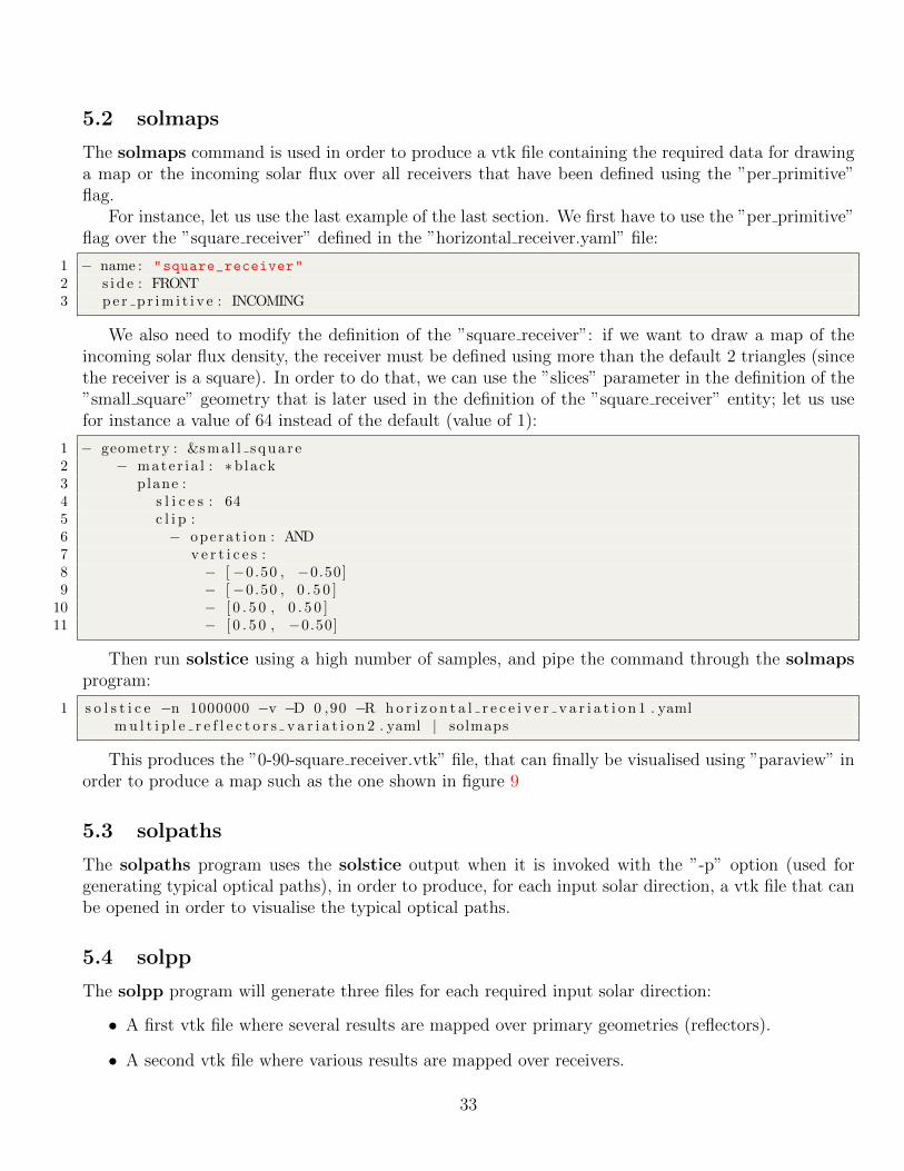
The solmaps command is used in order to produce a vtk file containing the required data for drawinga map or the incoming solar flux over all receivers that have been defined using the ”per primitive”flag.

For instance, let us use the last example of the last section. We first have to use the ”per primitive”flag over the ”square receiver” defined in the ”horizontal receiver.yaml” file:

1 − name : "square_receiver"

2 s i d e : FRONT3 pe r p r im i t i v e : INCOMING

We also need to modify the definition of the ”square receiver”: if we want to draw a map of theincoming solar flux density, the receiver must be defined using more than the default 2 triangles (sincethe receiver is a square). In order to do that, we can use the ”slices” parameter in the definition of the”small square” geometry that is later used in the definition of the ”square receiver” entity; let us usefor instance a value of 64 instead of the default (value of 1):

1 − geometry : &sma l l squa r e2 − mate r i a l : ∗black3 plane :4 s l i c e s : 645 c l i p :6 − opera t ion : AND7 v e r t i c e s :8 − [−0.50 , −0.50]9 − [−0.50 , 0 . 5 0 ]

10 − [ 0 . 5 0 , 0 . 5 0 ]11 − [ 0 . 5 0 , −0.50]

Then run solstice using a high number of samples, and pipe the command through the solmapsprogram:

1 s o l s t i c e −n 1000000 −v −D 0 ,90 −R ho r i z o n t a l r e c e i v e r v a r i a t i o n 1 . yamlmu l t i p l e r e f l e c t o r s v a r i a t i o n 2 . yaml | solmaps

This produces the ”0-90-square receiver.vtk” file, that can finally be visualised using ”paraview” inorder to produce a map such as the one shown in figure 9

5.3 solpaths

The solpaths program uses the solstice output when it is invoked with the ”-p” option (used forgenerating typical optical paths), in order to produce, for each input solar direction, a vtk file that canbe opened in order to visualise the typical optical paths.

5.4 solpp

The solpp program will generate three files for each required input solar direction:

• A first vtk file where several results are mapped over primary geometries (reflectors).

• A second vtk file where various results are mapped over receivers.

33

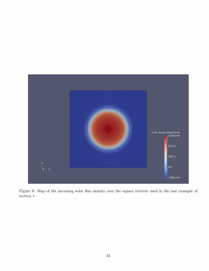
Figure 9: Map of the incoming solar flux density over the square receiver used in the last example ofsection 4

34

• A obj files used for the representation of geometries that are neither primary geometries, norreflectors.

This program uses two input files:

• A legacy simulation ouput file. For instance, over the last example of section 4:

1 s o l s t i c e −n 1000000 −D 0 ,90 −R ho r i z o n t a l r e c e i v e r . yaml −o s imul . txtmu l t i p l e r e f l e c t o r s . yaml

• The geometry of a solar plant, produced by solstice when invoked with the ”-g” options. Forinstance, over the last example of section 4:

1 s o l s t i c e −D 0 ,90 −R ho r i z o n t a l r e c e i v e r . yaml −g format=obj−o geometry . objmu l t i p l e r e f l e c t o r s . yaml

Then running the solpp command over the two files that result from previous commands:

1 so lpp geometry . obj s imul . txt

produces three files: ”0-90-primaries.vtk”, ”0-90-receivers.vtk” and ”0-90-miscellaneous.obj”. Fig-ure 10 shows the solar input flux over primary geometries, produces using the ”0-90-primaries.vtk” file.Figure 9 is a good example of what can be produced from the ”0-90-receivers.vtk” file. Figure 11 showsthe geometry stored in the ”0-90-miscellaneous.obj” file.

35

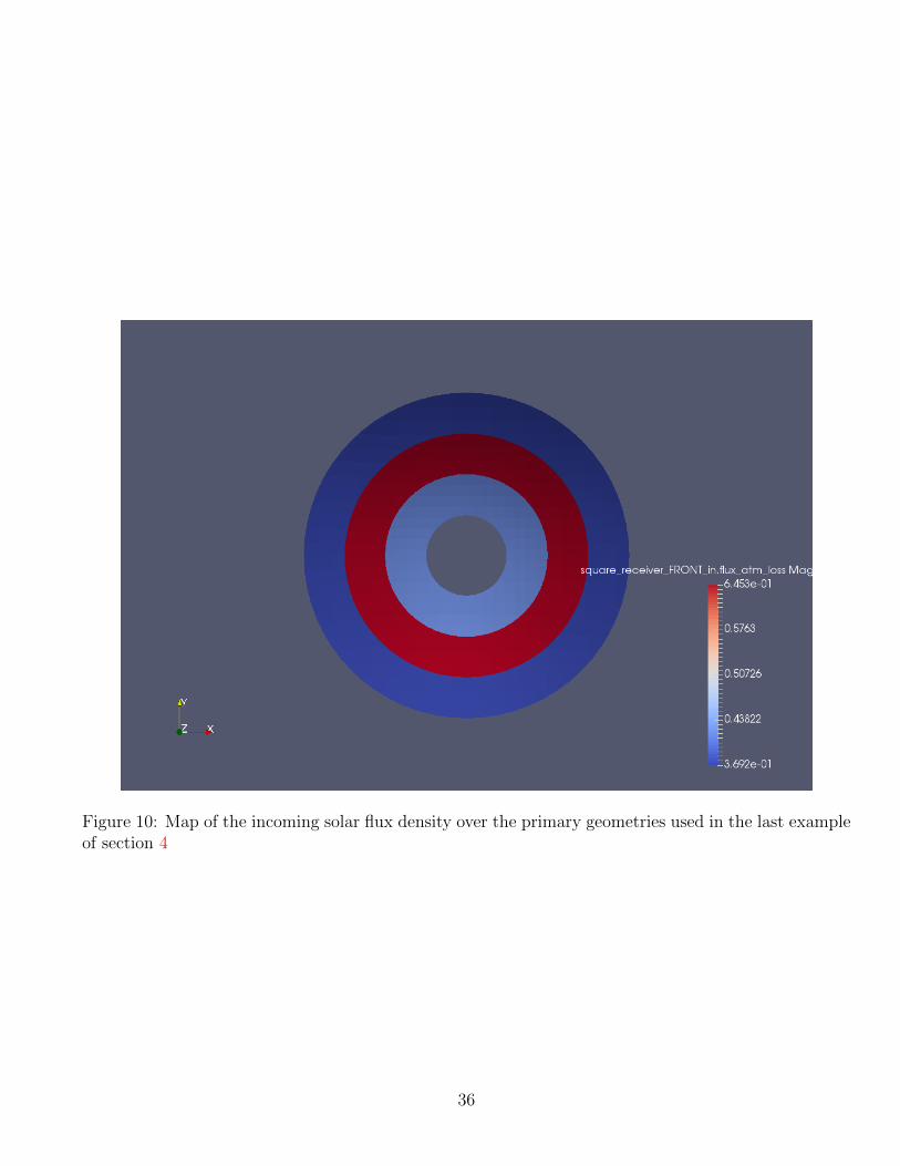
Figure 10: Map of the incoming solar flux density over the primary geometries used in the last exampleof section 4

36

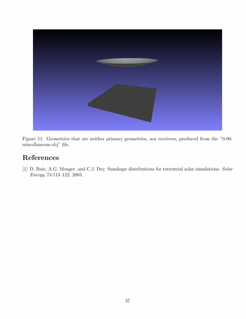
Figure 11: Geometries that are neither primary geometries, nor receivers, produced from the ”0-90-miscellaneous.obj” file.

References

[1] D. Buie, A.G. Monger, and C.J. Dey. Sunshape distributions for terrestrial solar simulations. SolarEnergy, 74:113–122, 2003.

37