solubility product - tonypaxton.orgmse307: solubility product 2018 (tony paxton and vivian tong)...

MSE307: Solubility Product 2018 (Tony Paxton and Vivian Tong) of 29

Solubility Product

1. Heat of formation and solubility of microalloying carbides and nitrides

We need to quantify the solubility of different transition metal carbides and nitrides,particularly in austenite at high temperature. This is because transition metal carbidesplay two crucial roles in microalloy and low alloy steels. (i) The more insoluble precipi-tates, for example TiC, TiN, NbN, exist at high temperature and act as austenite grainrefiners, say, during hot rolling. NbC also has a very marked effect in retarding dynamicrecrystallisation of the austenite. (ii) The more soluble compounds, for example V4C3 orVC, Mo2C and chromium carbides, will enter solution in the austenite during annealingand can be precipitated as nano-precipitates to improve strength during cooling andtransformation to ferrite, say, by interphase precipitation, or during tempering aftera quench to strengthen martensite. Iron carbide is the most soluble of all. Actuallythe more soluble compounds are those having the smaller enthalpies of formation (seeFigure 1). The alloy designer needs mathematical models and data that can be used topredict the distribution of carbon, nitrogen and transition metal alloying elements asfunctions of temperature—how much is in solution and how much exists as precipitates?We’d also like to know the size, shape, habit and orientation relation, but that’s anothermatter.

Figure 1: Heats of formation of some carbides and nitrides


1.1 Case of one microalloying element and single precipitate composition

Consider a chemical reaction

MmXn(ppt) = mM(sol) + nX(sol) (1.1.1)

which describes the dissolution of a carbide or nitride MmXn precipitate (ppt), for exam-ple NbN or V4C3 into solution (sol) in austenite at some temperature T . In equilibriumthe chemical potentials of components M and X are the same in the precipitate and inthe solution, so we have

µM,ppte = µM,sol and µX,ppte = µX,sol (1.1.2)

Expressing the chemical potentials in terms of standard chemical potential and activity,this becomes

µ◦M,ppte +RT ln aM,ppte = µ◦

M,sol +RT ln aM,sol

µ◦X,ppte +RT ln aX,ppte = µ◦

X,sol +RT ln aX,sol

Now, the chemical potential of the precipitate is, in view of (1.1.1) and (1.1.2)

µppte = mµM,ppte + nµX,ppte

= mµM,sol + nµM,sol

and therefore, again in terms of activity and standard state,

µ◦ppte +RT ln appte = mµ◦

M,sol +mRT ln aM,sol + nµ◦X,sol + nRT ln aX,sol

and rearranging this last equation, I get,

RT (m ln aM,sol + n ln aX,sol − ln appte) = µ◦ppte −mµ◦

M,sol − nµ◦X,sol

which is

RT lnamM,sol a

nX,sol

appte= −∆G◦

sol

= RT lnK

having defined∆G◦

sol = mµ◦M,sol + nµ◦

X,sol − µ◦ppte

as the standard Gibbs free energy of solution of the precipitate. This equation alsoserves to define the equilibrium constant K for the chemical reaction. I now have

amM,sol anX,sol = appte exp (−∆G◦

sol/RT )

The activity of a pure defect-free solid phase is constant (usually taken to be one) andfor a dilute solution Henry’s law tells us that the activity of a solute is proportionalto the concentration x expressed as an atomic fraction. The proportionality constants,γ, are called activity coefficients and are constant, independent of temperature andcomposition. So if xM and xX are the concentrations of M and X in the solid solutionand γM and γX are activity coefficients, we now have

(γMxM)m (γXxX)n = appte exp (−∆G◦sol/RT )

MSE307: Solubility Product 2018 (Tony Paxton and Vivian Tong) of 29TEM (Thin Foil)

[110](V, Mo)4C3//[100]α (100)(V, Mo)4C3//(100)α

[100](V, Mo)C//[100]α (200)(V, Mo)C//(110)α

α (V, Mo)C

α

(V, Mo)4C3

Fe-0.1C-0.2V

Baker -‐ Nu9ng Figure 2: Dark field images of (V,Mo)C interphase precipitates inan ultra high strength 0.1C–0.2V–0.5Mo steel (courtesy of PengGong and W. Mark Rainforth)

HRTEM images of nanometer-‐sized carbides obtained from the specimen isothermally treated at 650°C for 90min: (a) nanometer-‐sized (V, Mo)C; (b) the corresponding fast Fourier transformed (FTT) image from the same area of (a); (c) HRTEM FFT of nanometer sized carbide from red area in (a); (d) nanometer-‐sized (V, Mo)4C3; (e) the corresponding fast Fourier transformed (FTT) image from the same area of (d); (f) HRTEM FFT of nanometer sized carbide from red area in (a).

HRTEM images of nanometer-‐sized carbides obtained from the specimen isothermally treated at 650°C for 90min: (a) nanometer-‐sized (V, Mo)C; (b) the corresponding fast Fourier transformed (FTT) image from the same area of (a); (c) HRTEM FFT of nanometer sized carbide from red area in (a); (d) nanometer-‐sized (V, Mo)4C3; (e) the corresponding fast Fourier transformed (FTT) image from the same area of (d); (f) HRTEM FFT of nanometer sized carbide from red area in (a).

Figure 3: As figure 2 in high resolution: determination of orienta-tion relation (courtesy of Peng Gong and W. Mark Rainforth)


I can gather the three constants into a single constant, say, C = appte/γmMγ

nX, and write

xmM xnX = C exp (−∆G◦

sol/RT )

The weight percentages of M and X, which we conventionally write as [M] and [X] areproportional to the concentrations so the previous equation is equivalent to

[M]m[X]n = D exp (−∆G◦sol/RT )

in which D is another constant involving the atomic weights of the components andfactors of a hundred to convert to percent. I find

D = C × 1002 (m+ n)2

m2AM/AX + 2mn+ n2AX/AM

where AM and AX are the relative atomic masses (or atomic weights) of the elements Mand X. All this defines the solubility product, ks,

ks = [wt%M]m[wt%X]n

= [M]m[X]n (1.1.3)

= D exp (−∆G◦sol/RT )

Now I take logarithms to the base ten on both sides and I get

log ks = A−B/T (1.1.4a)

where the constants are

A = logD and B = ∆G◦sol/2.303R (1.1.4b)

Then all the constants including changes from natural to base 10 logs, standard statesand conversions to weight percent are accounted for by fitting experimental data toequation (1.1.4a). You will always find solubility product data in the metals handbooksand literature given by quoting the constants A and B for a particular carbide or nitridein austenite or ferrite. Of course the whole thing can be extended to multicomponentprecipitates, for example (V,Mo)(C,N) a carbonitride of vanadium and molybdenum(see Figures 2 and 3) but it’s a mess to write down and problems such as on page 7require a computer to solve.

Because of equation (1.1.4a) if we plot ln ks (or 2.303 log ks) against 1/T we get astraight line with a negative slope of magnitude ∆G◦

sol/R. This is called an Arrheniusplot; examples are shown in Figures 4 and 5.

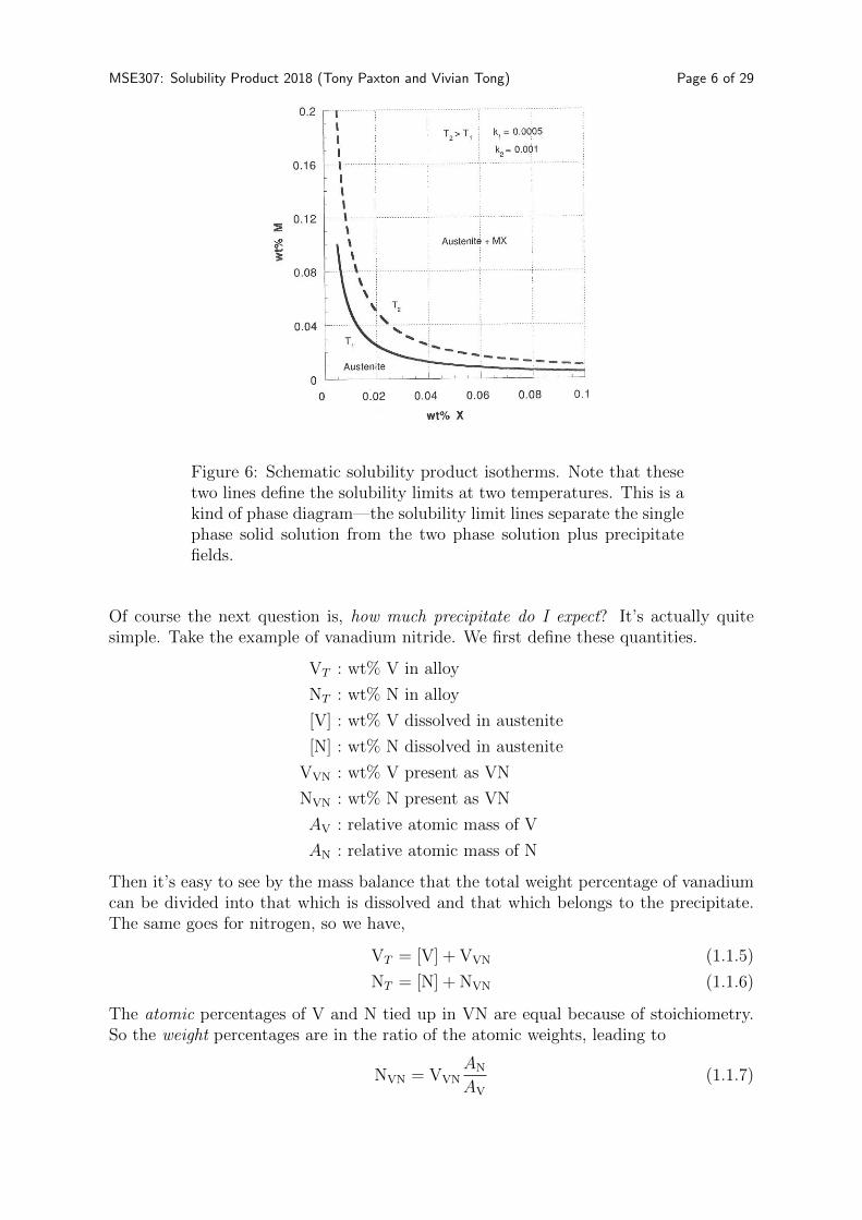
On the other hand, because of equation (1.1.3) it is clear that plotting [wt%M]m against[wt%X]n at any given temperature will result in a curve resembling a hyperbola asshown, for example, in the schematic in Figure 6. The way to interpret this graph isas follows. At the required temperature, say T2, and given concentrations of M and X(these could be, say, vanadium and nitrogen) we wish to know how much of the vandium


and nitrogen are in solution and how much are tied up in vanadium nitride precipitates.If we place a point on the graph corresponding to the known nominal compositions thenin equilibrium if that point falls to the left and below the curve the microstructure willbe a single phase austenite with V and N in solution. If the point falls above and to theright of the hyperbola then the microstructure will be a two phase mixture of VN andaustenite solid solution. The curve is therefore a graph of the solubility limit at thattemperature—if the concentrations of V and N lie on a point to the right and above thesolubility limit the that limit is exceeded and some of these elements must come out ofsolution and form precipitates.

Publ

ished

by

Man

ey P

ublis

hing

(c) I

OM

Com

mun

icatio

ns L

td

24?8. This shows the substantially higher solubility ofthe carbide than the nitride and the significant decreasein solubility in ferrite compared with austenite. A moredetailed discussion of the solubility of VC and VN inaustenite and VC in ferrite is provided by Gladman.3

For comparison, a selection made by Aronsson28 ofsolubility of the transition metal carbides and nitrides inaustenite, of importance in microalloyed steels, is givenin Fig. 3, where it is apparent that vanadium carbideand nitride are the most soluble carbide and nitride ofeach group. Strid and Easterling29 have also collectedrelevant solubility data.

An important aspect of most transition metal carbidesand nitrides, is that with few exceptions, they aremutually soluble, as is shown by the data presented byGoldschmidt.30 It has been suggested that this mutuallysolubility occurs when the atomic size differencebetween the two carbide or nitride forming elements isnot greater than 13%. Houghton31 was among the first

to acknowledge the effect of mutual solubility ofcarbides and nitrides in microalloyed steels. He pre-sented a quasi-regular solution thermodynamic modelwhich described the precipitation of complex carbidesand nitrides from austenite for two extreme cases:

(i) no mixing between precipitates(ii) complete miscibility while maintaining in both

cases equilibrium between precipitates andsolutes in austenite.

His results were then compared with those of othermodels, whose predictions are in general intermediatebetween (i) and (ii).

While the binary solubility equation approach is auseful guide, sophisticated methods have been evolvedusing dedicated software, which take into account the

1 Solubility of vanadium carbide in austenite and ferrite

2 Solubility of vanadium nitride in austenite and ferrite154

3 Solubility products, in atomic per cent, of carbides and

nitrides in austenite as function of temperature28

Table 1 Solubility of vanadium carbide in austenite and ferrite

Austenite Ferrite

Equation A B Type Ref. Equation A B Ref.

1 29500 6.72 VC 16 5 212 265 8.05 232 210 800 7.06 V4C3 21 6 27050 4.24 223 29400 5.65 V4C3 22 7 27667 4.57 14 26560 4.45 V4C3 18

Table 2 Solubility of vanadium nitride in austenite andferrite154

Austenite Ferrite

Equation A B Ref. Equation A B Ref.

8 27700 2.86 17 11 29700 3.90 179 28700 3.63 16 12 27061 2.26 2710 27840 3.02 26 13 27830 2.45 24

Baker Processes, microstructure and properties of V microalloyed steels

Materials Science and Technology 2009 VOL 25 NO 9 1085

Figure 4: Arrhenius plots of solubility products in austenite (left)and ferrite (right)

Figure 5: More Arrhenius plots of solubility product in iron. Notethat the most soluble carbides and nitrides are those lines towardsthe top of the figure—having the largest solubility products.


Figure 6: Schematic solubility product isotherms. Note that thesetwo lines define the solubility limits at two temperatures. This is akind of phase diagram—the solubility limit lines separate the singlephase solid solution from the two phase solution plus precipitatefields.

Of course the next question is, how much precipitate do I expect? It’s actually quitesimple. Take the example of vanadium nitride. We first define these quantities.

VT : wt% V in alloy

NT : wt% N in alloy

[V] : wt% V dissolved in austenite

[N] : wt% N dissolved in austenite

VVN : wt% V present as VN

NVN : wt% N present as VN

AV : relative atomic mass of V

AN : relative atomic mass of N

Then it’s easy to see by the mass balance that the total weight percentage of vanadiumcan be divided into that which is dissolved and that which belongs to the precipitate.The same goes for nitrogen, so we have,

VT = [V] + VVN (1.1.5)

NT = [N] + NVN (1.1.6)

The atomic percentages of V and N tied up in VN are equal because of stoichiometry.So the weight percentages are in the ratio of the atomic weights, leading to

NVN = VVNAN

AV

(1.1.7)


And, by definition of the solubility product we have

ks = [V][N] (1.1.8)

The rest is algebra. Let’s first find a formula for the amount of dissolved vanadium, [V].From (1.1.8) we have

[V] =ks[N]

(1.1.9)

and

[N] = NT − NVN

= NT − 14

51VVN

= NT − 14

51(VT − [V])

using (1.1.5) and (1.1.6) and then substituting (1.1.7). Then (1.1.9) leads to a quadraticequation for the amount of dissolved vanadium, namely,

1

51[V]2 +

(1

14NT − 1

51VT

)[V] − 1

14ks = 0 (1.1.10)

This can be solved using the usual formula for quadratic equations and once we have[V] we can find VVN and NVN, the amounts of vanadium and nitrogen that are tied upin the precipitate as functions of the nominal compositions, VT and NT , of V and Nand their atomic weights; and the solubility product which is a measurable function ofthe temperature. If we had more than one possible compound, or if we are interested incarbonitrides then the thermodynamic principles remain the same. The algebra becomesa lot more complicated and requires the solution of a number of simultaneous equations.The alloy designer uses commercial computer packages.

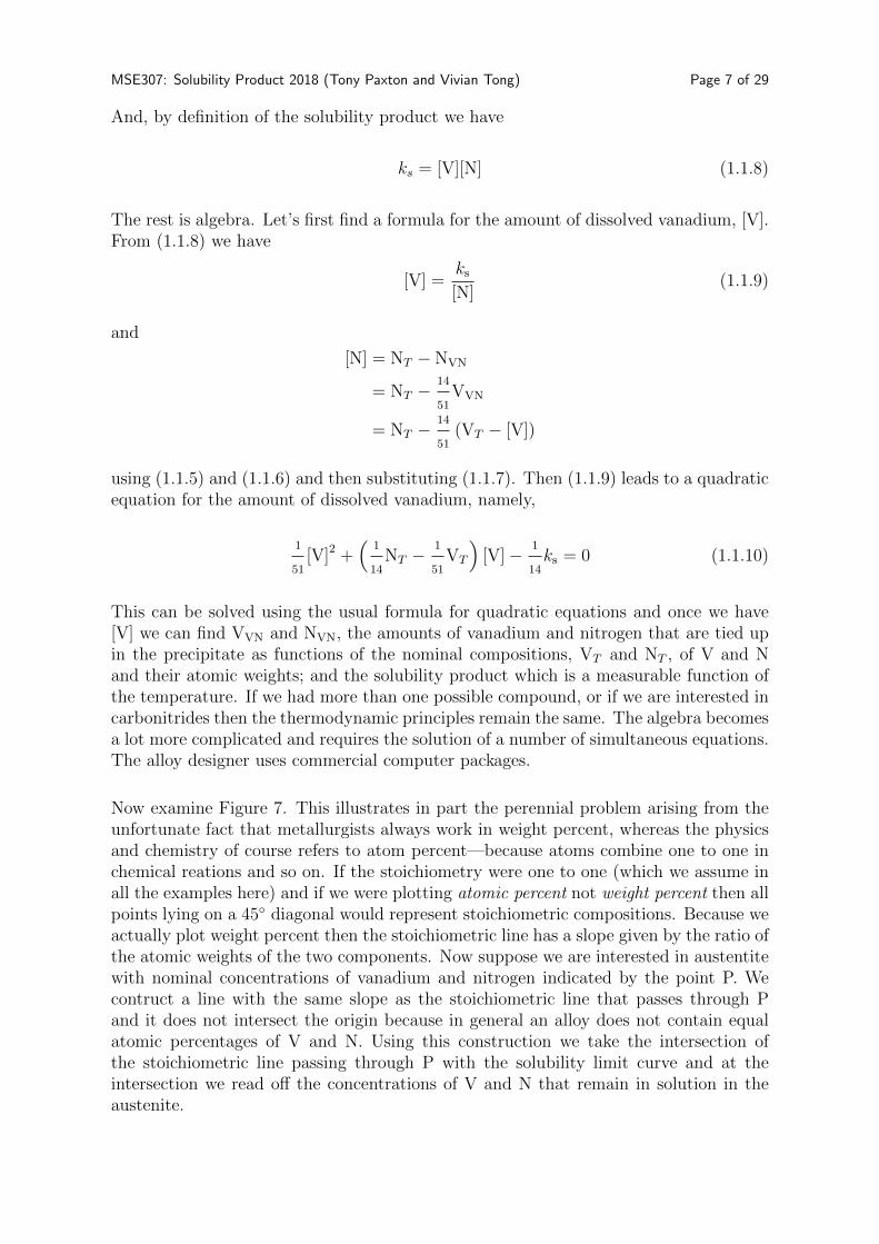
Now examine Figure 7. This illustrates in part the perennial problem arising from theunfortunate fact that metallurgists always work in weight percent, whereas the physicsand chemistry of course refers to atom percent—because atoms combine one to one inchemical reations and so on. If the stoichiometry were one to one (which we assume inall the examples here) and if we were plotting atomic percent not weight percent then allpoints lying on a 45◦ diagonal would represent stoichiometric compositions. Because weactually plot weight percent then the stoichiometric line has a slope given by the ratio ofthe atomic weights of the two components. Now suppose we are interested in austentitewith nominal concentrations of vanadium and nitrogen indicated by the point P. Wecontruct a line with the same slope as the stoichiometric line that passes through Pand it does not intersect the origin because in general an alloy does not contain equalatomic percentages of V and N. Using this construction we take the intersection ofthe stoichiometric line passing through P with the solubility limit curve and at theintersection we read off the concentrations of V and N that remain in solution in theaustenite.


Figure 7: Construction for the determination of the amounts of Vand N in solution and in precipitate. Note (A−B)/(D−C) = 51/14.

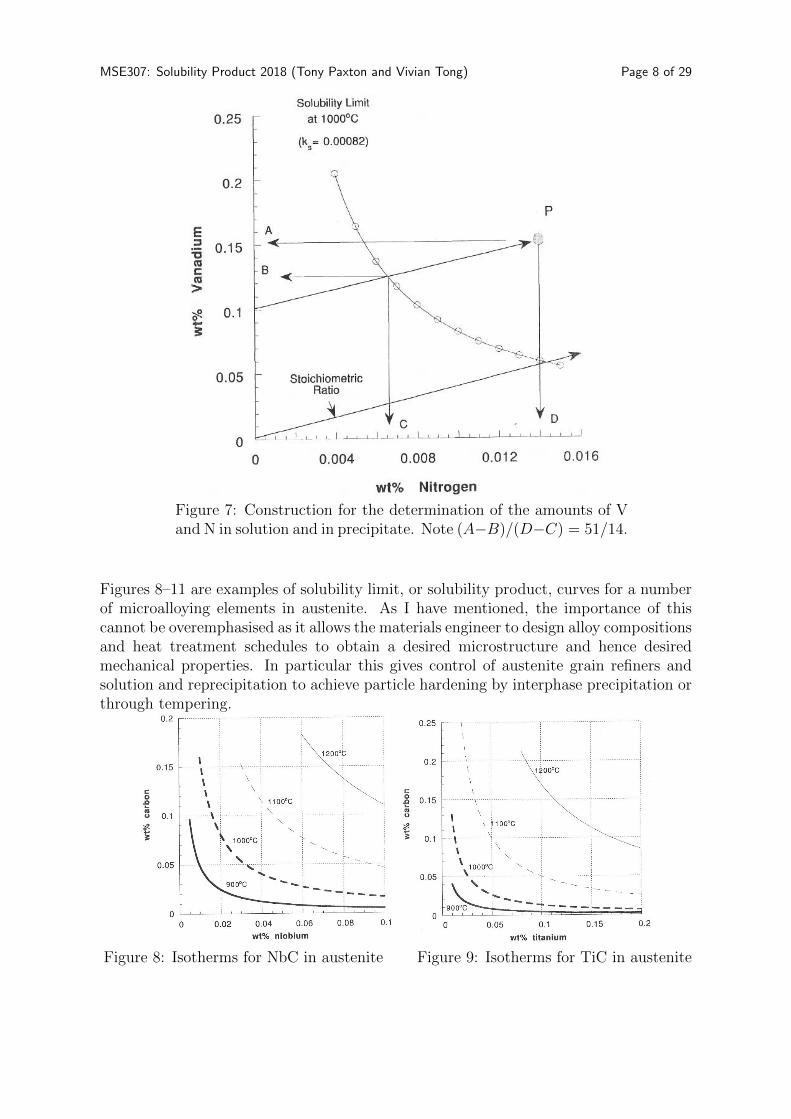
Figures 8–11 are examples of solubility limit, or solubility product, curves for a numberof microalloying elements in austenite. As I have mentioned, the importance of thiscannot be overemphasised as it allows the materials engineer to design alloy compositionsand heat treatment schedules to obtain a desired microstructure and hence desiredmechanical properties. In particular this gives control of austenite grain refiners andsolution and reprecipitation to achieve particle hardening by interphase precipitation orthrough tempering.

Figure 8: Isotherms for NbC in austenite Figure 9: Isotherms for TiC in austenite


Figure 10: Isotherms for VN in γ-phase 1.3% Mn steelFigure 11: Isotherms for AlN in austenite

Figure 12 illustrates what you have learned up to now. Suppose you are interested,for the sake of simplicity, in a steel with a single microalloying element, titanium, at0.1 wt%. How can you optimise hardening precipitates that form after cooling fromaustenite by varying the carbon concentration? The upper diagram shows solubilitylimits (products) at three temperatures. Imagine that the steel requires an isothermalanneal at 1200◦ during which all the Ti and C are to be dissolved so that they cansubsequently form, say, interphase precipitates as the austenite transforms to ferrite oncooling. You will need at least a stoichiometric amount of carbon or there won’t beenough to tie up all the Ti as TiC and some Ti must inevitably remain in solutionin the austenite and in the resulting ferrite—this may be fine if you are seeking somesolution hardening. This is the situation if the carbon concentration falls in region Ain the lower diagram. As the carbon increases from zero the amount of Ti and C thatwill be available to combine will increase until the stoichiometric line intersects the Ticoncentration. Note that as we increase the carbon concentration the equivalent of ourpoint P in Figure 7 is moving to the right along the horizontal broken line in the upperdiagram. In region A there is more Ti than C atomic percent; beyond the stoichiometricpoint there is more C than Ti atomic percent. Therefore in region B, the amount ofcarbide that can form is fixed and at its maximum amount, given the 0.1 wt% of Ti; theremaining carbon will probably form iron or other carbides on cooling—no bad thing,perhaps. At the boundary of regions B and C the point P moves from the left and belowthe solubility limit to above and to its right so that at the soaking temperature of 1200◦

the equilibrium microstructure is austenite plus TiC. This means that not all the Ti andcarbon become dissolved and that TiC that forms at 1200◦ is likely to grow coarse and beuseless at particle hardening. At the same time these coarse precipitates tie up some ofthe Ti and C that would otherwise be available to form fine interphase precipitates andin consequence the cooled alloy will have the TiC fraction “limited by solubility”. Theconclusion is that in this case using any carbon concentration in the range of region Bwill give optimum fine carbide fraction, since if the carbon concentration is less thecarbide fraction is limited by stoichiometry and if it’s greater some Ti and C will betied up as useless (possibly even deleterious) large second phase particles.


Figure 12: Effect of stoichiometry on the precipitation of TiC in amicroalloyed steel

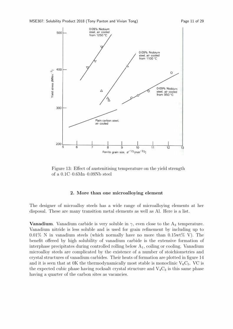
Figure 13 shows how these ideas are exploited in the design of fine grain miroalloyedniobium steels. Notice that there are two effects of increasing the annealing temperaturebefore air cooling. (i) The yield stress increases overall. (ii) The Hall-Petch slopeincreases. This is because at the higher annealing temperatures, more NbC is dissolvedand therefore available for interphase precipitation in the ferrite in order to contributeto the particle hardening.


Figure 13: Effect of austenitising temperature on the yield strengthof a 0.1C–0.6Mn–0.09Nb steel

2. More than one microalloying element

The designer of microalloy steels has a wide range of microalloying elements at herdisposal. These are many transition metal elements as well as Al. Here is a list.

Vanadium. Vanadium carbide is very soluble in γ, even close to the A3 temperature.Vanadium nitride is less soluble and is used for grain refinement by including up to0.01% N in vanadium steels (which normally have no more than 0.15wt% V). Thebenefit offered by high solubility of vanadium carbide is the extensive formation ofinterphase precipitates during controlled rolling below A1, coiling or cooling. Vanadiummicroalloy steels are complicated by the existence of a number of stoichiometries andcrystal structures of vanadium carbides. Their heats of formation are plotted in figure 14and it is seen that at 0K the thermodynamically most stable is monoclinic V6C5. VC isthe expected cubic phase having rocksalt crystal structure and V4C3 is this same phasehaving a quarter of the carbon sites as vacancies.


3

a) b) c) d)e)

FIG. 1. Structures of the simulated unit cells for a) VC, b) V4C3-Cubic, c) V4C3-Hexagonal, d) V6C5-Hexagonal and e)V6C5-Monoclinic. The darker atoms represent carbon and the lighter ones vanadium.

TABLE I. Calculation details for the DFT calculations performed. The units for the smearing temperature and the cut-offenergy are Eh

Calculation details

k-point k-points Bands Smearing Cut-offgrid temperature energy

V 18×18×18 190 12 0.001 36C 19×19×19 400 32 0.001 36VC 9×9×9 85 15 0.001 36V4C3-Cubic 8×8×8 20 48 0.001 39V4C3-Hexagonal 7×7×1 25 144 0.001 36V6C5-Hexagonal 4×4×2 16 192 0.0009 36V6C5-Monoclinic 3×2×2 6 252 0.001 36γ − Fe 5×5×5 63 272 0.0005 46

-0.6

-0.5

-0.4

-0.3

-0.2

-0.1

0

0 0.2 0.4 0.6 0.8 1

∆H

f[e

V/ato

m]

Molar fraction of carbon, xC

V

VC

V4C3-Cubic

V4C3-Hexagonal

V6C5

C

FIG. 2. Calculated binary V-C phase diagram at 0 K and 0 Pa.The lines show the convex hull connecting stable phases.

The energies are calculated within the normalised vol-ume range [0.8, 1.2] with a step of 0.05. The results ofthe calculations in terms of the formation enthalpy areshown in Fig. 3. We find that hexagonal V4C3 is moreenergetically favourable than cubic V4C3. As noted ear-lier, hexagonal and monoclinic V6C5 are degenerate in

energy47. The coefficient BEOS0 of the fit, correspondingto the zero pressure bulk modulus is presented in TableIV. A reasonably good agreement is found with publishedtheoretical27,31,32,34,51 and experimental values52. In thecases of VC and cubic V4C3 the largest errors are 1.8%and 0.9%, respectively.

VII. ELASTIC PROPERTIES

Components of the Voigt stiffness matrix were calcu-lated using the stress-strain method.53 The procedure isbased on Hooke’s law, σσσ = CCCεεε, where σσσ is the measuredstress tensor, εεε the Green-Lagrange stress tensor, andCCC the stiffness tensor. The method is divided into thefollowing steps:

1. The system is structurally relaxed using the BFGSalgorithm until all stresses are minimised.

2. Six different deformation gradients are applied—oneat a time—to the relaxed structure in order to modify in-dependently each component of the deformation vector.For each deformation gradient, four different magnitudesare used, namely –0.01. –0.005, 0.005 and 0.01.

3. A relaxation of the atoms is done for each of the24 previously deformed configurations without modifyingthe geometry of the unit cell. The resulting stresses aremeasured.

Figure 14: Heats of formation of competing vanadium carbidephases, calculated using first principles quantum mechanics (den-sity functional theory).

Figure 15 shows the wide differences in solubility product, especially at high tempera-ture, in comparing VC and V4C3.

Figure 15: Solubility limits of vanadium and carbon based on cubicVC (solid lines) and V4C3 (broken lines). This is only consistentwith figure 14 if the V4C3 is taken to be hexagonal, not cubic.


Niobium. Carbonitrides dissolve only at higher soaking temperatures, and so particlestrengthening is restricted. Principally the carbonitrides act as γ grain refiners and verymarkedly supress recystallisation of the austenite under controlled rolling (Ti and Vhave similar but less effective roles). The change in solubility in the range 900–1300◦Cleads to significant deformation induced precipitation.

Titanium. TiN is very insoluble and will precipitate in the liquid steel to promotegrain refinement. Whatever Ti remains after TiN precipitation will result in TiC whichhas similiar solubility to NbC. Ti also is a sulphide former and so will dissolve in MnSparticles and reduce their ductility during hot rolling, thus preventing their elongation.

Aluminium addition as a deoxidant has to some extent been superseded by vacuummelting. Any Al not combined into alumina and taken off from the liquid remains toprovide AlN precipitates, having a relatively low solubility product. AlN has a differentcrystal structure compared to the common transition metal carbonitrides and so itprovides a “mutually exclusive” precipitate system (see section 2.1, below).

Molybdenum is primarily added to improve hardenability, but it will combine withvanadium carbonitride to form VxMo1−xCzN1−z (see figure 3)

This all means that the treatment in section 1.1 is too elementary for the general mi-croalloyed steel. We need to consider the equilibrium between more than one microalloyelement, carbon and nitrogen and one or more, possibly complex, carbonitrides. How-ever, if you keep your head, you will see that as in section 1.1, the mathematics whilemessy-looking is really very easy and only involves solving quadratic, cubic or quarticequations. The last two, of course, require a computer or graphical solution. So take adeep breath and study sections 2.1 and 2.2 below.

We study two cases in these notes. The simpler is the case in which two (or more) mutu-ally exclusive compounds are precipitated. This is the situation in which the compoundshave different crystal structures and are regarded as simultaneously in equilibrium withthe austenite matrix. The second, rather more difficult problem, is the one in whichone or more precipitates exist in equilibrium and are miscible, by virtue of their havingthe same crystal structure, containing more than one microalloy element or more thanone interstitial element (C or N). This latter case divides into two: the case of a singletransition metal carbonitride and the case of complex carbonitrides.

2.1 Mutually exclusive precipitates

If two or more compounds may precipitate having different crystal structures then we canconsider a number of chemical reactions such as (1.1.1) as occuring independently andretaining the same solubility products as if the others were not occurring. It is expectedthat this is the case in vanadium microalloy steels although it is not yet known whethermore than one of the vanadium carbides in figure 14 are to be found simultaneously inthe same steel. There is currently some evidence of cubic VC and cubic V4C3 being


found in the same steel but this is not necessarily a case of mutual exclusivity if weregard these as the same phase having variable carbon vacancy concentrations. Thiswould then amount to a third scenario in addition to the two discussed in the previousparagraph and we will not discuss this much further in these notes.

Instead I will use the example of hexagonal AlN existing in equilibrium with cubic VNat some temperature in austenite. We write two reactions as in equation (1.1.1),

AlN(ppt) = Al(sol) + N(sol) kA = [Al][N] (2.1.1a)

VN(ppt) = V(sol) + N(sol) kV = [V][N] (2.1.1a)

The solubility products are those of the individual reactions as taken from measurementsin ternary Fe-V-N and Fe-Al-N alloys. Actually kA � kV and so if sufficient Al werepresent in the steel then it will tie up a stoichiometric amount of N in AlN up to thesolubility limit given by kA. Any remaining N could then result also in VN precipitationif the solubility limit kV is exceeded. Therefore the alloy designer can manipulate theamounts of VN and AlN precipitates by adjusting the weight percentages of V, Al andN, and by choosing appropriate soaking and rolling temperatures.

Essentially as in section 1.1 we are tasked with finding out, at a given temperature,how much of each microalloy element is present in solution and how much is tied upas precipitate in equilibrium. In the case of just one microalloy element, V, and oneinterstitial element, N, we arrived rather easily at equation (1.1.10). In the case ofmutually exclusive precipitates only, we may use the simplification that the activities ofthe precipitates are one as before since they exist as immiscible pure phases which haveseparate crystal structures. Let us now proceed to a solution.

The total nitrogen content in weight percent is

NT = [N] + NAlN + NVN

namely the sum of the contributions to the total weight percentages from that in solution(so called free nitrogen), and those tied up in the separate chemical compounds. Becauseof the 1:1 stoichiometry we also know that

NAlN =14

27AlAlN

NVN =14

51VVN

because the atomic weights of N, Al and V are 14, 27 and 51. Combining these lastthree we have,

NT = [N] +14

27AlAlN +

14

51VVN

The weight percent of Al present as AlN is the same as the difference between the totalAl, AlT , and the dissolved Al; and similarly for the V and so we write,

AlAlN = AlT − [Al]

VVN = VT − [V]


and putting these into the previous equation results in

NT = [N] +14

27(AlT − [Al]) +

14

51(VT − [V]) (2.1.2)

The two nitrides must each be present in amounts consistent with the independentsolubility products, and so we can substitute for [V] and [N] from (2.1.1) and henceeliminate these in favour of the known solubility products to obtain a closed equationfor the dissolved nitrogen. Firstly the last equation becomes, on substitution from (2.1.1)

NT = [N] +14

27

(AlT − kA

[N]

)+

14

51

(VT − kV

[N]

)I can multiply both sides by [N] and collect terms and I arrive at

1

14[N]2 +

(1

27AlT +

1

51VT − 1

14NT

)[N] −

(1

27kA +

1

51kV

)= 0 (2.1.3)

It is worthwhile to compare this to (1.1.10). It is also a simple quadratic equation thatcan be solved analytically in terms of known quantities: the composition of the steeland the solubility products at the soaking temperature. There will not be a solutionif there is only one precipitate and there may be nonsensical solutions turning up—forexample if dissolved amounts predicted by equations (2.1.1) turn out to be greater thatthe total amounts then there will be negative quantities of precipitate predicted!

While there is a number of approximations attendant on the derivation of (2.1.3) itspredictions have been found to be in accord with experiment as shown in the examplein figure 16.

Figure 16: Comparison between prediction and experiment of freenitrogen in Al-V-N steels


As in the simpler case of section (1.1), remember that once you have [N] by solutionof equation (2.1.3) then you can use mass balance and (2.1.1) to find the amounts ofAl and V in both solution and in the two separate compounds and find the amount ofnitrogen remaining in solution.

You can go further and use the equations that you have to construct a phase diagramshowing the one, two and three phase regions as functions of the microalloy contents.Proceed as follows. From (2.1.1), since [N] is the same in both equations because thenitrogen is simultaneously in equilibrium with both precipitates we know that

[Al]

[V]=kAkV

(2.1.4)

I now take [V] from this equation and I take [N] from (2.1.1a) and put them into (2.1.2)which leads to

NT =kA[Al]

+14

27(AlT − [Al]) +

14

51

(VT − kV

kA[Al]

)

I now mulitply through by [Al] and collect powers in [Al] and I get this quadraticequation, (

14

27+

14

51

kVkA

)[Al]2 −

(14

27AlT +

14

51VT − NT

)[Al] − kA = 0

So far this is just another equation like (2.1.3) but this time for the dissolved Al ratherthan N. But if I take the special case that the dissolved Al content is equal to the totalAl content, that is,

[Al] = AlT = Alpb (2.1.5)

then this defines Alpb as the weight percent of Al at the phase boundary between the twophase γ+VN and the three phase γ+AlN+VN fields. In other words Alpb is the largestconcentration of Al that can be added to a vanadium containing steel while still pre-venting the precipitation of AlN. Now if I apply the condition (2.1.5) to equation (2.1.2)then the second term vanishes and as before using (2.1.1a) and (2.1.4) I find

14

51

kVkA

Al2pb −(

14

51VT − NT

)Alpb − kA = 0

which I can solve for Alpb. I can follow an identical procedure to find Vpb and so getthe locus of the γ+AlN / γ+AlN+VN phase boundary. This construction is shown infigure 17.


Figure 17: Calculated phase diagram

2.2 Carbonitrides

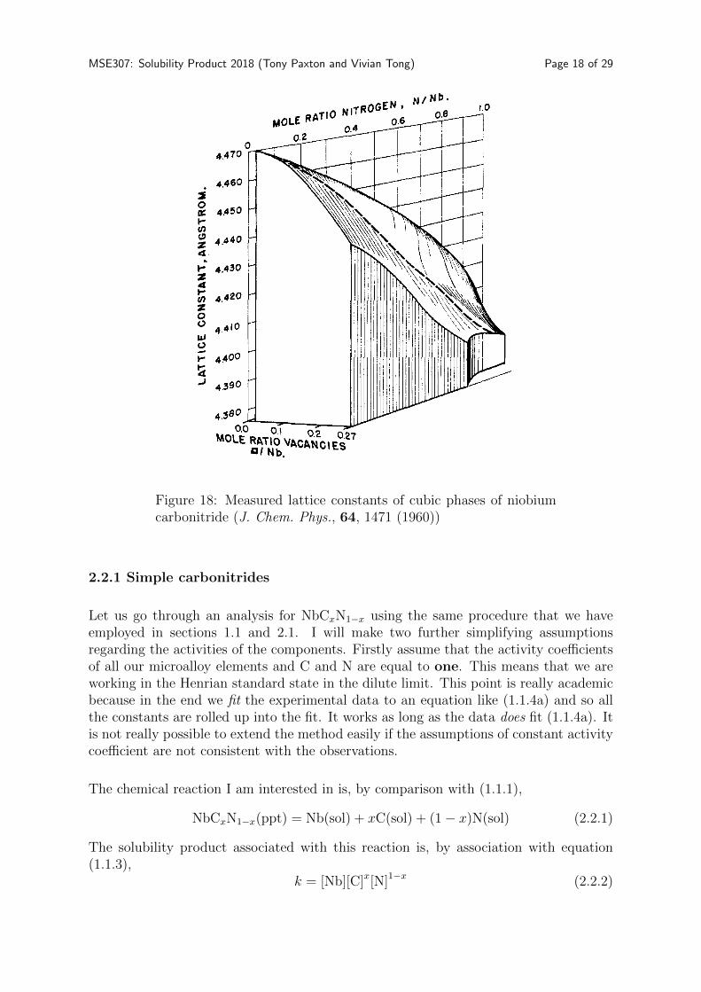
A simple carbonitride has a chemical formula MmCnNp. In complex carbonitrides, thesymbol M is taken to mean a combination of transition metal elements. In cases wherethese phases occur in the rocksalt structure which consists of two interpenetrating fcclattices, then we expect the chemical formula to be MCxN1−x and 0 < x < 1. Thetransition metal atoms occupy one sublattice and the interstitial elements the other.(Equivalently you can think of this as an fcc transition metal with C and N atomsoccupying octahedral interstices—see Barrett and Massalski.) All of the sites in the firstsublattice are occupied (possibly by one of several transition metal elements randomlyplaced). The second sublattice is occupied by C and N in the ratio x/1−x. But not allsites might be occupied. Most transition metal carbonitrides are sub-stoichiometric—afraction of the sites are vacant. Figure 18 shows this effect in niobium carbonitridesand the resulting measured lattice parameters. This means that we should write ourchemical formula as MCxNy 1−x−y, where stands for vacancy. As I mentioned in thefirst paragraph of section 2.1, this amounts to a third scenario which we don’t look athere. Instead we will focus for simplicity on simple or complex carbonitrides having a1:1 ratio of transition metal to interstitial atoms.

MSE307: Solubility Product 2018 (Tony Paxton and Vivian Tong) of 291476 E. K. STORMS AND N. H. KRIKORIAN Vol. 64

r' a

4 f

0

I- # 0 z I-

I- # 1 0 0 ur

t-

2

2 E

4 470

.

Fig. 3.--Lattice parameter us. composition in the system NbN-NbC.

portant, when dealing with materials like niobium carbide to specify the amounts of oxygen or nitrogen present. Either of these impurities will change the lattice parameter if dissolved or, at least, make the sample appear richer in the metal. Thus, the various solid phase boundaries would appear to be shifted to the left from their true positions. For example, a sample having an analyzed composition of NbCo.eoo, which contains 0.2 weight % nitrogen would actually be NbCo.elr, the amount of niobium combined with nitrogen as NbN being sub- tracted. With this in mind, it became necessary to determine how rapidly oxygen and nitrogen would be eliminated from niobium carbide by heating and, to a limited extent, \\-hat effect the remaining impurity n-ould have. This is also an important (~orol1iir.c- t o earlier m r k by the authors on the variatioti of KliC lattice parameter with composition.

Two cxperiments 'vITere made and the results are listed in Tables V and JrI. In the first, separate samples of commercial grade NbC (Fansteel) were subJected to various heating times and temperatures in ai1 effort to produce samples containing a smaller and smaller amount of impurity. The powder mas contained in a graphite crucible during t hc: heating. Apparent)ly heating a t 1900' for 20 minutes is sufficient to drive o f f most of the oxygen and iiitrogen contained in a previously re- acted sample. In Fig. 2 a comparison is made between the lattice parameter curve previously reported4 and the values for these impure materials. The arrow from each point, indicates the magnitude of the nitrogen correction. It is impossible to correct for oxygen since the form of the oxide is unknown. Txo conclusions can be dram-n : oxygen and nitrogen can be readily eliminated from NbC a t the expense of free and combined carbon, and samples still containing these impurities will lie to the right of the published curve.

TABLE V HEATING OF IMPURE KbC

Uncor. Wt. % impurities combined Free

Temp., Tilue, C to Nb car- OXY- Kitro- nun. ratio bon Fen gen no, A. " C .

KO heating 0.895 0.33 0.28 0.66 4.4697 1300 5 ,903 .06 . I 5 .54 3.4681 1650 10 ,924 .OO ,075 .17 4.4670 1900 20 ,918 .OO ,052 .05 4.4658 2200 120 ,917 . O O ,017 .(JO 4.4661

TABLE VI HEATING OF CONTAMINATED S h C

Starting compn. Xb = 87.81 at. R c = 9 2 : N = 2 36 0 = 0 . 5 8 (10 = 4 4(30 -

100.00

Heated for 1 hr. at 1450'

Heated slowly to 1920' and continued for 30 min.

r i n a l compn. Xb = 9 0 . 5 3 c = 9.02 N = 0.30 0 = 0.02

99.87

ao = 4.4G8 -!- extra lines

(10 = 4 446 + extralines

-

Uncor. compn. XbCo.7; Cor. compn. NbCo.7~ assuming all nitrogen as S b S ~ . o o

Table VI shows the results of the second experiment. Here, nitrogen and oxygen were added as Nbn' and Nb206 to pure XbC. Again the amount of nitrogen was reduced by a factor of ten and the oxygen essentially eliminated by heating in vacuo a t 1920' for about 30 minutes. Based on the change in lattice parameter, heating at 1450' for 1 hour, apparently had very little effect.

It is not known how rapidly these impurities would be eliminated in the region near SbzC. The impurity mould, however, have the same effect on the analyzed composition as descrihcd above.

The effect of nitrogen in the KhC system has recently been reported by Braiicr 2nd Lesser.I5 Figure 3 shows a line drawing of a niodd constnlcted by plotting their data as the ratios C/Sb, N/Kh and vacancies/ljb on the ternary axes and the lattice parameter on the wrtical axis. The lattire parameter curve for pure KbC is bnccd 011 Fig. 2. The surface thus created show that dissolved nitrogen causes a lowering of the lattice pnrametcr but in a manner dependent 011 the number of vacancies in the lattice. A small amouiit of nitrogen will cause a smaller decrease in a. at NbCo.9 than mould be produced if it were dissolved in IVbC0.7, for example.

In addition, this figure makes it clear that a study of lattice parameter in any binary system in which the starting materials have a range of homo- geneity is not unique unless the amount of vacancy is specified. For example, Duivez and Ode1116 give the variation in a. for several biliary systems including NbC-SbK. Based on the lattice parameter gixlen, their XbC was nearly stoichiometric (4.470 A. = SbCo99), but the K b S appar$ntly contained a large number of vacancies (4.379 A. g

(15) G. Rraoer and R. Lesser, 2. Metallkunde, 60, 167 (1959). (16) P. Dunez and F. Odell, J. Electrochem. Soc. , 97, 299 (19501.

Figure 18: Measured lattice constants of cubic phases of niobiumcarbonitride (J. Chem. Phys., 64, 1471 (1960))

2.2.1 Simple carbonitrides

Let us go through an analysis for NbCxN1−x using the same procedure that we haveemployed in sections 1.1 and 2.1. I will make two further simplifying assumptionsregarding the activities of the components. Firstly assume that the activity coefficientsof all our microalloy elements and C and N are equal to one. This means that we areworking in the Henrian standard state in the dilute limit. This point is really academicbecause in the end we fit the experimental data to an equation like (1.1.4a) and so allthe constants are rolled up into the fit. It works as long as the data does fit (1.1.4a). Itis not really possible to extend the method easily if the assumptions of constant activitycoefficient are not consistent with the observations.

The chemical reaction I am interested in is, by comparison with (1.1.1),

NbCxN1−x(ppt) = Nb(sol) + xC(sol) + (1 − x)N(sol) (2.2.1)

The solubility product associated with this reaction is, by association with equation(1.1.3),

k = [Nb][C]x[N]1−x (2.2.2)


so this depends on the stoichiometry of the carbonitride through x which is unknownas a function of composition and temperature. If I break down the reaction (2.2.1) intotwo half reactions I can assert that (2.2.1) is the sum of these two reactions

xNbC(in NbCN) = xNb(sol) + xC(sol) (2.2.3a)

(1 − x)NbN(in NbCN) = (1 − x)Nb(sol) + (1 − x)N(sol) (2.2.3b)

(I am using NbCN as a shorthand for NbCxN1−x.) These two reactions taking placesimultaneously assert an equilibrium in which in (2.2.3a) Nb and C in solution are inequilibrium with the component NbC and in which in (2.2.3b) Nb and N in solutionare in equilibrium with the component NbN. Here we imply that NbC and NbN aretwo components that make up the carbonitride. The fact that I’ve multiplied throughby x and 1 − x doesn’t change the reactions and so the solubility products for the tworeactions are

k1 =[Nb][C]

activity of NbC in NbCN(2.2.3c)

k2 =[Nb][N]

activity of NbN in NbCN(2.2.3d)

We now make our second simplifying assumption and assume that the carbonitride is anideal solid solution of NbC and NbN so that the activities of each of those componentsare just x and 1−x respectively which are the concentrations of each of these componentsof the carbonitride. Since we assume an ideal solution of NbN and NbC in NbCxN1−x

the activities in (2.2.3c) and (2.2.3d) are just the concentrations x and 1−x so solubilityproducts for the two half reactions are

k1 = [Nb][C]/x (2.2.3e)

k2 = [Nb][N]/(1 − x) (2.2.3f)

I raise the first of these equations to the power x and the second to the power 1−x andmultiply the two resulting equations together,

kx1k1−x2 =

1

xx(1 − x)1−x[Nb]x[C]x[Nb]1−x[N]1−x

=1

xx(1 − x)1−x[Nb][C]x[N]1−x (2.2.4)

Comparing the solubility product (2.2.2) for the reaction (2.2.1) with (2.2.4) it is seento be equal to

k = kx1k1−x2 xx(1 − x)1−x (2.2.5)

or, if you prefer, by taking logarithms of both sides,

log k = x log k1 + (1 − x) log k2 + x log x+ (1 − x) log(1 − x) (2.2.6)

This has the very pleasing structure of the weighted sum of the two solubility productsfor reactions (2.2.2) plus an ideal entropy of mixing term. From this sublime height it


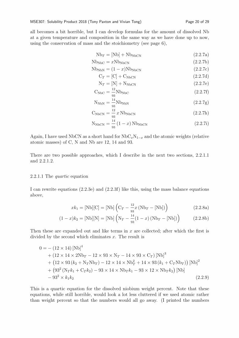
all becomes a bit horrible, but I can develop formulas for the amount of dissolved Nbat a given temperature and composition in the same way as we have done up to now,using the conservation of mass and the stoichiometry (see page 6),

NbT = [Nb] + NbNbCN (2.2.7a)

NbNbC = xNbNbCN (2.2.7b)

NbNbN = (1 − x)NbNbCN (2.2.7c)

CT = [C] + CNbCN (2.2.7d)

NT = [N] + NNbCN (2.2.7e)

CNbC =12

93NbNbC (2.2.7f)

NNbN =14

93NbNbN (2.2.7g)

CNbCN =12

93xNbNbCN (2.2.7h)

NNbCN =14

93(1 − x) NbNbCN (2.2.7i)

Again, I have used NbCN as a short hand for NbCxN1−x and the atomic weights (relativeatomic masses) of C, N and Nb are 12, 14 and 93.

There are two possible approaches, which I describe in the next two sections, 2.2.1.1and 2.2.1.2.

2.2.1.1 The quartic equation

I can rewrite equations (2.2.3e) and (2.2.3f) like this, using the mass balance equationsabove,

xk1 = [Nb][C] = [Nb](

CT − 12

93x (NbT − [Nb])

)(2.2.8a)

(1 − x)k2 = [Nb][N] = [Nb](

NT − 14

93(1 − x) (NbT − [Nb])

)(2.2.8b)

Then these are expanded out and like terms in x are collected; after which the first isdivided by the second which eliminates x. The result is

0 = − (12 × 14) [Nb]4

+ (12 × 14 × 2NbT − 12 × 93 × NT − 14 × 93 × CT ) [Nb]3

+(12 × 93 (k2 + NTNbT ) − 12 × 14 × Nb2

T + 14 × 93 (k1 + CTNbT ))

[Nb]2

+(932 (NTk1 + CTk2) − 93 × 14 × NbTk1 − 93 × 12 × NbTk2

)[Nb]

− 932 × k1k2 (2.2.9)

This is a quartic equation for the dissolved niobium weight percent. Note that theseequations, while still horrible, would look a lot less cluttered if we used atomic ratherthan weight percent so that the numbers would all go away. (I printed the numbers


deliberately small on pages 14–16 so as not to obscure the structure any more thannecessary.)

Once [Nb] is known then the amount of Nb tied up as carbonitride is

NbNbCN = NbT − [Nb]

Then the stoichiometry of the carbonitride is found as follows. Combining (2.2.7d)and (2.2.3e) with the stoichiometric formula (2.2.7h) we find

x = CT

(k1

[Nb]+

12

93NbNbCN

)−1

= CT

(k1

[Nb]+

12

93(NbT − [Nb])

)−1

(2.2.10)

Once we have the amount of dissolved Nb from solving (2.2.9) and the stoichiometry ofthe carbonitride (2.2.10) then we can find the amount of Nb, C and N in solution andtied up as carbonitride from (2.2.7a), (2.2.7d–e) and (2.2.7h–i).

2.2.1.2 The quadratic equation

The solubility products, k1 and k2, depend on x and we don’t know how to get themfrom experiment. However we do know the solubility products for the binary NbC andNbN precipitates, from separate measurements of Fe-Nb-C and Fe-Nb-N alloys,

NbC(ppt) = Nb(sol) + C(sol) ; kC = [Nb]C[C]C (2.2.11a)

NbN(ppt) = Nb(sol) + N(sol) ; kN = [Nb]N[N]N (2.2.11b)

By comparison of (2.2.3e) and (2.2.3f) with (2.2.11), we are tempted to write

kC = xk1 (2.2.12a)

kN = (1 − x)k2 (2.2.12b)

However this is not correct, as I’ve indicated with subscripts “C” and “N” in (2.2.11): theamounts of carbon and nitrogen in solution, [C] and [N], in equilibrium with NbCxN1−x

in a Fe-Nb-C-N alloy are not the same as the amount of carbon [C]C in equilibrium withNbC in a Fe-Nb-C alloy and the amount of nitrogen [N]N in equilibrium with NbN in aFe-Nb-N alloy.

But if I admit the assertion (2.2.12) then I can replace the left hand sides of (2.2.8) withkC and kN. I then eliminate x between these two equations and obtain

1

93[Nb]2 +

(1

14NT +

1

12CT − 1

93NbT

)[Nb] − 1

12kC − 1

14kN = 0 (2.2.13)

This is a quadratic equation that can be solved to find the amount of dissolved Nb.

Once we have that then we can find the amount of Nb tied up as precipitate, us-ing (2.2.7a),

NbNbCN = NbT − [Nb]


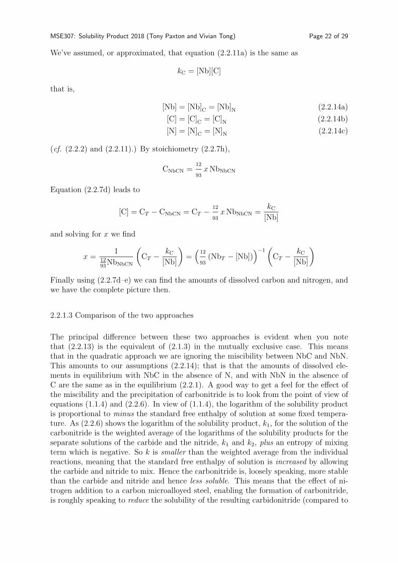
We’ve assumed, or approximated, that equation (2.2.11a) is the same as

kC = [Nb][C]

that is,

[Nb] = [Nb]C = [Nb]N (2.2.14a)

[C] = [C]C = [C]N (2.2.14b)

[N] = [N]C = [N]N (2.2.14c)

(cf. (2.2.2) and (2.2.11).) By stoichiometry (2.2.7h),

CNbCN =12

93xNbNbCN

Equation (2.2.7d) leads to

[C] = CT − CNbCN = CT − 12

93xNbNbCN =

kC[Nb]

and solving for x we find

x =1

1293

NbNbCN

(CT − kC

[Nb]

)=(

12

93(NbT − [Nb])

)−1(

CT − kC[Nb]

)Finally using (2.2.7d–e) we can find the amounts of dissolved carbon and nitrogen, andwe have the complete picture then.

2.2.1.3 Comparison of the two approaches

The principal difference between these two approaches is evident when you notethat (2.2.13) is the equivalent of (2.1.3) in the mutually exclusive case. This meansthat in the quadratic approach we are ignoring the miscibility between NbC and NbN.This amounts to our assumptions (2.2.14); that is that the amounts of dissolved ele-ments in equilibrium with NbC in the absence of N, and with NbN in the absence ofC are the same as in the equilibrium (2.2.1). A good way to get a feel for the effect ofthe miscibility and the precipitation of carbonitride is to look from the point of view ofequations (1.1.4) and (2.2.6). In view of (1.1.4), the logarithm of the solubility productis proportional to minus the standard free enthalpy of solution at some fixed tempera-ture. As (2.2.6) shows the logarithm of the solubility product, k1, for the solution of thecarbonitride is the weighted average of the logarithms of the solubility products for theseparate solutions of the carbide and the nitride, k1 and k2, plus an entropy of mixingterm which is negative. So k is smaller than the weighted average from the individualreactions, meaning that the standard free enthalpy of solution is increased by allowingthe carbide and nitride to mix. Hence the carbonitride is, loosely speaking, more stablethan the carbide and nitride and hence less soluble. This means that the effect of ni-trogen addition to a carbon microalloyed steel, enabling the formation of carbonitride,is roughly speaking to reduce the solubility of the resulting carbidonitride (compared to


the carbide and nitride) and hence to promote precipitation, or equivalently to raise thetemperature at which all the Nb is dissolved.

The quartic approach was taken by Hudd et al., J. Iron and Steel Institute, 209, 121(1971). However because k1 and k2 are not known as functions of x, Hudd et al. assumedthat

k1 = kC (2.2.15a)

k2 = kN (2.2.15b)

That is, for k1 and k2 they used published solubility product data from Fe-Nb-C andFe-Nb-N alloys. This is arguably an even more drastic approximation than (2.2.11) and(2.2.12) used in the quadratic approach, namely,

k1 = kC/x (2.2.16a)

k2 = kN/(1 − x) (2.2.16b)

because at least here the solubility products implicitly depend on x as they should.We could argue that in principle the quartic approach is the more rigorous, but theapproximation that needs to be made to solve it is more drastic than the approximationof exclusive carbide and nitride, albeit combined into a single stoichiometry carbonitrideprecipitate. But we see now that this is incorrect.

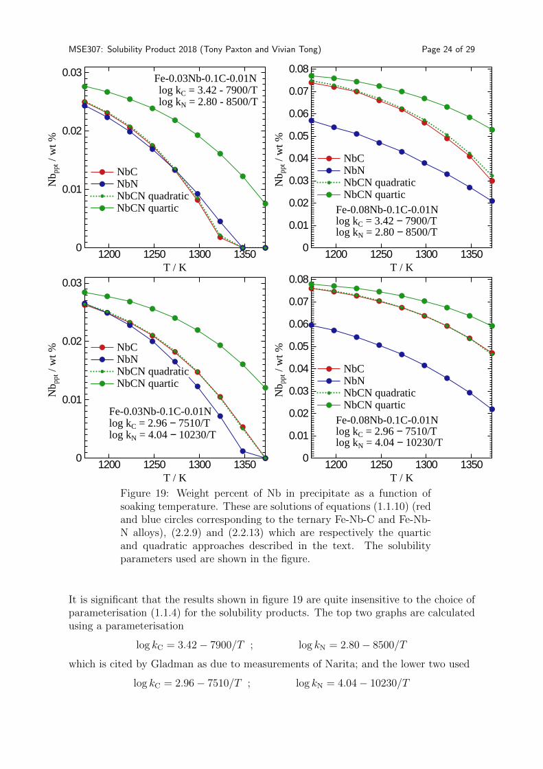
Figure 19 illustrates the comparison using as examples Fe-0.03Nb-0.1C-0.01N and Fe-0.08Nb-0.1C-0.01N steels. The red and blue circles correspond to solutions of equa-tion (1.1.10) for the cases that either nitrogen or carbon are absent, and show theweight precent of Nb expected to be tied up in precipitate as functions of the austenitis-ing temperature. For the quaternary alloys we show solutions obtained from the quartic(as solid lines) and quadratic (as dotted lines) connecting the green circles.

The quadratic approach, which amounts to the mutually exclusive case, practicallypredicts the same amount of precipitate as for the case of the Fe-Nb-C alloy. This isbecause (2.2.13) essentially reduces to (1.1.10) because kN is an order of magnitudesmaller than kC (figure 5) and NT is an order of magnitude smaller than CT .

On the other hand, the quartic approach properly takes account of the enthopy ofmixing. As argued above this has the effect of increasing the thermodynamic stabilityof the NbCxN1−x and so it’s solubility is less and a greater amount of precipitate ispredicted compared to the mutually exclusive (quadratic) approximation. There stillremains the fact the ansatz (2.2.15) cannot be right. The qualitative features of thetheory are evident in figure 19, but this does not mean that the quantitative predictionsare correct. It may be possible to calculate k1 and k2 from electronic structure theory.It may also be possible to do experiments as suggested by equations (2.2.3e) and (2.2.3f)in which as a function temperature, using different compositions of Fe-Nb-C-N alloys,both the equilibrium concentrations of dissolved N and C and the stoichiometry, x, ofthe NbCxN1−x can be measured.


1200 1250 1300 13500

0.01

0.02

0.03

T / K

Nb p

pt /

wt %

NbCNbNNbCN quadraticNbCN quartic

Fe-0.03Nb-0.1C-0.01Nlog kC = 3.42 - 7900/Tlog kN = 2.80 - 8500/T

1200 1250 1300 13500

0.01

0.02

0.03

0.04

0.05

0.06

0.07

0.08

T / KN

b ppt

/ w

t %


Fe-0.08Nb-0.1C-0.01Nlog kC = 3.42 − 7900/Tlog kN = 2.80 − 8500/T

1200 1250 1300 13500

0.01

0.02

0.03

T / K

Nb p

pt /

wt %



1200 1250 1300 13500

0.01

0.02

0.03

0.04

0.05

0.06

0.07

0.08

T / K

Nb p

pt /

wt %



Figure 19: Weight percent of Nb in precipitate as a function ofsoaking temperature. These are solutions of equations (1.1.10) (redand blue circles corresponding to the ternary Fe-Nb-C and Fe-Nb-N alloys), (2.2.9) and (2.2.13) which are respectively the quarticand quadratic approaches described in the text. The solubilityparameters used are shown in the figure.

It is significant that the results shown in figure 19 are quite insensitive to the choice ofparameterisation (1.1.4) for the solubility products. The top two graphs are calculatedusing a parameterisation

log kC = 3.42 − 7900/T ; log kN = 2.80 − 8500/T

which is cited by Gladman as due to measurements of Narita; and the lower two used

log kC = 2.96 − 7510/T ; log kN = 4.04 − 10230/T


which are the parameters quoted by Hudd et al. Since the assumption (2.2.15) is thatk1 = kC and k2 = kN and since we expect that k1 < kC and k2 < kN as argued above,then the solubility of NbCxN1−x is overestimated and we expect that actual amounts ofprecipitate to be even larger than predicted.

2.2.2 Complex carbonitrides

Imagine a steel with composition A wt%Ti, B wt%Nb, C wt%C and D wt%N. Incomparison to equations (2.2.3a,b) we have these equilibria,

TiC(in TiNbCN) = Ti(sol) + C(sol) ; k1 = [Ti][C]/aTiC (2.2.17a)

NbC(in TiNbCN) = Nb(sol) + C(sol) ; k2 = [Nb][C]/aNbC (2.2.17b)

TiN(in TiNbCN) = Ti(sol) + N(sol) ; k3 = [Ti][N]/aTiN (2.2.17c)

NbN(in TiNbCN) = Nb(sol) + N(sol) ; k4 = [Nb][N]/aNbN (2.2.17d)

in which a is the activity of the precipitate. Again, we may not take these as being one.Consider the dissolution of a complex carbide of Ti and Nb, and a complex nitride ofTi and Nb,

TixNb1−xC(ppt) = xTi(sol) + (1 − x)Nb(sol) + C(sol) (2.2.18a)

TiyNb1−yN(ppt) = yTi(sol) + (1 − y)Nb(sol) + N(sol) (2.2.18b)

As in the case of the simple carbonitride we envisage the formation of the complexcarbonitride in two stages: first the formation of the carbide and the nitride (2.2.18),followed by their mixing to form the carbonitride. The formation of the complex car-bonitride is described by the equilibrium,

Tixz+y(1−z)Nb(1−x)z+(1−y)(1−z)CzN1−z(ppt) =

zxTi(sol) + z(1 − x)Nb(sol) + zC(sol)+(1 − z)yTi(sol)+

(1 − z)(1 − y)Nb(sol) + (1 − z)N(sol)

in which we essentially mix z moles of (2.2.18a) with (1 − z) moles of (2.2.18b).

As in section 2.2.1 we assume that the complex carbonitride is an ideal solid solution ofthe component complex carbides and nitrides then we can assert that

aTiC = xz (2.2.19a)

aNbC = z(1 − x) (2.2.19b)

aTiN = y(1 − z) (2.2.19c)

aNbN = (1 − y)(1 − z) (2.2.19d)

We proceed in the same vein as before exploiting the mass balance identities, stoichiome-tries and the irritating atomic weight ratios. The weight percentage of N in the austenitematrix is [N] and so the weight percent nitrogen in the carbonitride is D− [N], and theweight percent carbon in the carbonitride is (12/14)(D − [N])z/(1 − z). The weightpercent of Ti in the carbonitride is the sum of that weight percent that came from the


formation of TiC in the first step of the thought experiment plus that coming from theTiN,

wt%Ti in carbonitride = Ticarbonitride =48

14(D − [N])

xz + y(1 − z)

1 − z

in the same way

wt%Nb in carbonitride = Nbcarbonitride =93

14(D − [N])

(1 − x)z + (1 − y)(1 − z)

1 − z

Now we can find the matrix compositions of C, Ti and Nb in terms of [N] and the alloycomposition and stoichiometry of the carbonitride (remember that the steel compositionis A wt%Ti, B wt%Nb, C wt%C and D wt%N, so in our notation, A = TiT , B = NbT ,C = CT and D = NT ),

[C] = C − 12

14(D − [N])

z

1 − z

[Ti] = A− 48

14(D − [N])

xz + y(1 − z)

1 − z

[Nb] = B − 93

14(D − [N])

(1 − x)z + (1 − y)(1 − z)

1 − z

Putting these into the second column of equations (2.2.17) for the solubility productswe get, bearing in mind (2.2.19),

k1 = [Ti][C]/aTiC

=1

xz

(A− 48

14(D − [N])

xz + y(1 − z)

1 − z

)(C − 12

14(D − [N])

z

1 − z

)(2.2.20a)

k2 = [Nb][C]/aNbC

=1

z(1 − x)

(B − 93

14(D − [N])

z(1 − x) + (1 − y)(1 − z)

1 − z

)×(

C − 12

14(D − [N])

z

1 − z

)(2.2.20b)

k3 = [Ti][N]/aTiN

=1

y(1 − z)

(A− 48

14(D − [N])

xz + y(1 − z)

1 − z

)[N] (2.2.20c)

k4 = [Nb][N]/aNbN

=1

(1 − y)(1 − z)

(B − 93

14(D − [N])

z(1 − x) + (1 − y)(1 − z)

1 − z

)[N](2.2.20d)

If y is made the subject of (2.2.20c) and this then substituted into (2.2.20a, b and d)then, after making x the subject of these, three further equations result,

x =f1([N], z)

f2([N], z)(2.2.21a)

x =f3([N], z)

f4([N], z)(2.2.21b)

x =f5([N], z)

f6([N], z)(2.2.21c)


in which the six functions as defined in (2.2.21) are

f1 = A(1 − z)k3

(C(1 − z) − 12

14z (D − [N])

)f2 = z

((1 − z)k1

((1 − z)k3 +

48

14[N] (D − [N])

)+

48

14(D − [N]) k3

(C(1 − z) − z

12

14(D − [N])

))f3 =

{((1 − z)k3 +

48

14[N] (D − [N])

)(93

14(D − [N]) −B(1 − z)

)−A[N](1 − z)

93

14(D − [N])

}(c(1 − z) − 12

14z (D − [N])

)+ z(1 − z)2 k2

((1 − z)k3 +

93

14[N] (D − [N])

)f4 = z(1 − z)

{(1 − z)k2

((1 − z)k3 +

48

14[N] (D − [N])

)+

93

14(D − [N])

(C(1 − z) − z

12

14(D − [N])

)}f5 = B(1 − z)[N]

{(1 − z)k3 +

48

14[N] (D − [N])

}−{

(1 − z)k4 +93

14[N] (D − [N])

}{(1 − z)2 k3 +

48

14[N] (D − [N]) − A(1 − z)[N]

}+ z(1 − z)[N] (D − [N])

(48

14k4 −

93

14k3

)f6 = z(1 − z)[N] (D − [N])

(48

14k4 −

93

14k3

)We seek values of [N], the dissolved nitrogen concentration, and z, the fraction of theinterstitial sites that are occupied by carbon (as opposed to nitrogen—there are novacancies in this problem) such that equations (2.2.21) are consistent; that is, suchthat each of those three ratios, f1/f2, f3/f4 and f5/f6, is equal to a number, x, whichmust of course be between zero and one (since it is the fraction of transition metal sitesoccupied by Ti, as opposed to Nb). Equating the three equations (2.2.21) results in justtwo independent equations,

f1f2

=f3f4

f1f2

=f5f6

equivalentlyf1 f4 = f2 f3

f1 f6 = f2 f5

Two further functions of [N] and z are defined, namely,

F1 = f1 f4 − f2 f3

F2 = f1 f6 − f2 f5

and it follows that when both of these are zero a solution is found as long as it resultsin sensible values of [N] and z, namely that 0 < [N] < D and 0 < z < 1.


This provides the basis of a computed solution of the problem of determining the amountand the stoichiometry of the complex carbonitride in the steel of a given compostionand temperature.

The procedure is illustrated in figure 20. The computer selects systematically trialvalues of z (between zero and one) from which [N] is found by iteration. For each pair(z, [N]) the functions f1 to f6 are evaluated and hence functions F1 and F2. In figure 20,the solid line shows the concentration of free nitrogen, [N], as a function of z for whichF1 = 0, and the broken line shows the same for which F2 = 0. For those values of [N]and z for which both F1 and F2 are zero, namely at the interesection of the two lines, wehave a solution of the problem at the chosen composition and temperature. Of courseit assumed that data are available for the solubility products, k1 to k4, for the ternaryequilibria (2.2.17).

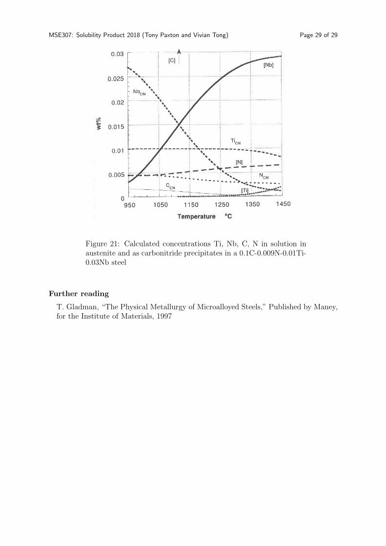
Figure 21 shows a full solution of the problem for a 0.1C-0.009N-0.01Ti-0.03Nb steel(that is A = 0.01, B = 0.03, C = 0.1, D = 0.009). The calculated weight percent-ages of the components in solution and in carbonitride are shown as a function of thetemperature. CN is shorthand for carbonitride.

Figure 20: Schematic illustration of the solution to equations(2.2.21)


Figure 21: Calculated concentrations Ti, Nb, C, N in solution inaustenite and as carbonitride precipitates in a 0.1C-0.009N-0.01Ti-0.03Nb steel

Further reading

T. Gladman, “The Physical Metallurgy of Microalloyed Steels,” Published by Maney,for the Institute of Materials, 1997

solubility product - tonypaxton.orgmse307: solubility product 2018 (tony paxton and vivian tong)...

Documents