solucionario ecuaciones diferenciales dennis zill 9ed
TRANSCRIPT

Complete Solutions Manual
A First Course in Differential Equations with Modeling Applications
Ninth Edition
Dennis G. ZillLoyola Marymount University
Differential Equations with Boundary-Vary Problems
Seventh Edition
Dennis G. ZillLoyola Marymount University
Michael R. CullenLate of Loyola Marymount University
By
Warren S. WrightLoyola Marymount University
Carol D. Wright
* ; BROOKS/COLEC E N G A G E Learning-
Australia • Brazil - Japan - Korea • Mexico • Singapore • Spain • United Kingdom • United States
www.elsolucionario.net

http://www.elsolucionario.net
www.elsolucionario.net

Table of Contents1 Introduction to Differential Equations 1
2 First-Order Differential Equations 27
3 Modeling with First-Order Differential Equations 86
4 Higher-Order Differential Equations 137
5 Modeling with Higher-Order Differential Equations 231
6 Series Solutions of Linear Equations 274
7 The Laplace Transform 352
8 Systems of Linear First-Order Differential Equations 419
9 Numerical Solutions of Ordinary Differential Equations 478
10 Plane Autonomous Systems 506
11 Fourier Series 538
12 Boundary-Value Problems in Rectangular Coordinates 586
13 Boundary-Value Problems in Other Coordinate Systems 675
14 Integral Transforms 717
15 Numerical Solutions of Partial Differential Equations 761 Appendix I Gamma function 783
Appendix II Matrices 785
www.elsolucionario.net

3.ROOKS/COLEC 'N G A G E Learn ing”
i 2009 Brooks/Cole, Cengage Learning
ALL RIGHTS RESERVED. No part of this work covered by the copyright herein may be reproduced, transmitted, stored, or used in any form or by any means graphic, electronic, or mechanical, including but not limited to photocopying, recording, scanning, digitizing, taping, Web distribution, Information networks, or information storage and retrieval systems, except as permitted under Section 107 or 108 of the 1976 United States Copyright Act, without the prior written permission of the publisher except as may be permitted by the license terms below.
For product information and technology assistance, contact us at Cengage Learning Customer & Sales Support,
1-800-354-9706
For permission to use material from this text or product, submit all requests online at www.cengage.com/permissions
Further permissions questions can be emailed to permissionreq uest@cenga ge. com
ISBN-13. 978-0-495-38609-4 ISBN-10: 0-495-38609-X
Brooks/Cole10 Davis Drive Belmont, CA 94002-3098 USA
Cengage Learning is a leading provider of customized [earning solutions with office locations around the globe, including Singapore, the United Kingdom, Australia, Mexico, Brazil, and Japan. Locate your local office at: international.cengage.com/region
Cengage Learning products are represented in Canada by Nelson Education, Ltd.
For your course and learning solutions: visit academic.cengage.com
Purchase any of our products at your local college store or at our preferred online store www.ichapters.com
NOTE’. UNDER NO C\RCUMST ANCES MAY TH\S MATERIAL OR AMY PORTION THEREOF BE SOLD, UCENSED, AUCTIONED, OR OTHERWISE REDISTRIBUTED EXCEPT AS MAY BE PERMITTED BY THE LICENSE TERMS HEREIN.
READ IMPORTANT LICENSE INFORMATION
Dear Professor or Other Supplement Recipient:
Cengage Learning has provided you with this product (the “Supplement' ) for your review and, to the extent that you adopt the associated textbook for use in connection with your course (the ‘Course’ ), you and your students who purchase the textbook may use the Supplement as described below. Cengage Learning has established these use limitations in response to concerns raised by authors, professors, and other users regarding the pedagogical problems stemming from unlimited distribution of Supplements.
Cengage Learning hereby grants you a nontransferable license to use the Supplement in connection with the Course, subject to the following conditions. The Supplement is for your personal, noncommercial use only and may not be reproduced, posted electronically or distributed, except that portions of the Supplement may be provided to your students IN PRINT FORM ONLY in connection with your instruction of the Course, so long as such students are advised that they
may not copy or distribute any portion of the Supplement to any third party. You may not sell, license, auction, or otherwise redistribute the Supplement in any form. We ask that you take reasonable steps to protect the Supplement from unauthorized use. reproduction, or distribution. Your use of the Supplement indicates your acceptance of the conditions set forth in this Agreement. If you do not accept these conditions, you must return the Supplement unused within 30 days of receipt.
All rights (including without limitation, copyrights, patents, and trade secrets) in the Supplement are and will remain the sole and exclusive property of Cengage Learning and/or its licensors. The Supplement is furnished by Cengage Learning on an "as is” basis without any warranties, express or implied. This Agreement will be governed by and construed pursuant to the laws of the State of New York, without regard to such State’s conflict of law rules.
Thank you for your assistance in helping to safeguard the integrity of the content contained in this Supplement. We trust you find the Supplement a useful teaching tool
:"tcd in Canada 1 3 4 5 6 7 11 10 09 08
www.elsolucionario.net

1 Introduction to Differential Equations
1. Second order; linear
2. Third order; nonlinear because of (dy/dx)4
3. Fourth order; linear
4. Second order; nonlinear bccausc of cos(r + u)
5. Second order; nonlinear because of (dy/dx)2 or 1 + (dy/dx)2
6. Second order: nonlinear bccausc of R~
7. Third order: linear
8. Second order; nonlinear because of x2
9. Writing the differential equation in the form x(dy/dx) -f y2 = 1. we sec that it is nonlinear in y
because of y2. However, writing it in the form (y2 — 1 )(dx/dy) + x = 0, we see that it is linear in x.
10. Writing the differential equation in the form u(dv/du) + (1 + u)v = ueu wc see that it is linear in
v. However, writing it in the form (v + uv — ueu)(du/dv) + u — 0, we see that it, is nonlinear in ■Ji
l l . From y = e-*/2 we obtain y' = — \e~x'2. Then 2y' + y = —e~X//2 + e-x/2 = 0.
12. From y = | — |e-20* we obtain dy/dt = 24e-20t, so that
% + 20y = 24e~m + 20 - |e_20t) = 24.clt \ 'o 5 /
13. R'om y = eix cos 2x we obtain y1 = 3e^x cos 2x — 2e3* sin 2a? and y” = 5e3,x cos 2x — 12e3,x sin 2x, so
that y" — (k/ + l?>y = 0.
14. From y = — cos:r ln(sec;r + tanrc) we obtain y’ — — 1 + sin.Tln(secx + tana:) and
y" = tan x + cos x ln(sec x + tan a?). Then y" -f y = tan x.
15. The domain of the function, found by solving x + 2 > 0, is [—2, oo). From y’ = 1 + 2(x + 2)_1/2 we
1
www.elsolucionario.net

Exercises 1.1 Definitions and Terminology
have
{y - x)y' = (y - ®)[i + (20 + 2)_1/2]
= y — x + 2(y - x)(x + 2)-1/2
= y - x + 2[x + 4(z + 2)1/2 - a;] (a: + 2)_1/2
= y — x + 8(ac + 2)1;/i(rr + 2)~1/2 = y — x + 8.
An interval of definition for the solution of the differential equation is (—2, oo) because y
defined at x = —2.
16. Since tan:r is not defined for x = 7r/2 + mr, n an integer, the domain of y = 5t£v.
An interval of definition for the solution of the differential equation is (—7r/10,7T/10 . A:,
interval is (7r/10, 37t/10). and so on.
17. The domain of the function is {x \ 4 — x2 ^ 0} or {x\x ^ —2 or x ^ 2}. Prom y' — 2.:: -= -
we have
An interval of definition for the solution of the differential equation is (—2,2). Other
(—oc,—2) and (2, oo).
18. The function is y — l/y/l — s ins. whose domain is obtained from 1 — sinx ^ 0 or . = 1 T
An interval of definition for the solution of the differential equation is (tt/2. 5tt/2 A:.. .
is (57r/2,97r/2) and so on.
19. Writing ln(2X — 1) — ln(X — 1) = t and differentiating implicitly we obtain
2 dX 1 dX
2 X - 1 dt X - l dt
{a; | 5x ^ tt/2 + 7i-7r} or {;r | x ^ tt/IO + mr/5}. From y' — 25sec2 §x we have
y' = 25(1 + tan2 5x) = 25 + 25 tan2 5a: = 25 + y2.
the domain is {z | x ^ tt/2 + 2?i7r}. From y' = —1(1 — sin x) 2 (— cos.x) we have
2y' = (1 — sin;r)_ ‘?/’2 cos# = [(1 — sin:r)~1//2]3cos:r - f/3cosx.
(2X - 1)(X - 1) dt
IX— = -C2X - 1)(X - 1) = (X - 1)(1 - 2X .
2X - 2 - 2X + 1 dX _
2www.elsolucionario.net
Exercises 1.1 Definitions and Terminology
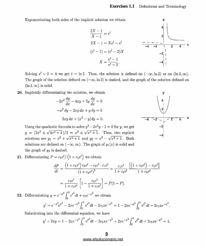
Exponentiating both sides of the implicit solution we obtain
2 X - 1
x
----- = elX - l
2 X - 1 = Xel - ef
(e* - 1) = (e‘ - 2)X
ef' — 1
- 4 - 2
X =e*- 2 '
-2
- 4
Solving e* — 2 = 0 we get t = In2. Thus, the solution is defined on (—oc.ln2) or on (In2, oo).
The graph of the solution defined on (—oo,ln2) is dashed, and the graph of the solution defined on
(In 2. oc) is solid.
20. Implicitly differentiating the solution, we obtain y
—x2 dy — 2xy dx + y dy — 0
2 xy dx + (a;2 — y)dy = 0.
Using the quadratic formula to solve y2 — 2x2y — 1 = 0 for y, we get
y = (2x2 ± V4;c4 +4)/2 = a’2 ± vV 1 + 1 . Thus, two explicit
solutions are y\ = x2 + \A'4 + 1 and y-2 = x2 — V.x4 + 1. Both
solutions are defined on (—oo. oc). The graph of yj (x) is solid and
the graph of y-2 is daalied.
21. Differentiating P = c\?} } ( l + cie^ we obtain
dP _ ( l + cie*) cie* - cie* • cie* _ Cie« [(l + cie‘) - cie4]
(1 + cie*)"eft
Ci
1 + CI&-
CiC
1 + ci ef
1 + cief
= P( 1 - P).
1 + cie(
2 PX ,2 ,222. Differentiating y = e~x / e: dt + c\ e~x we obtain
Jo
* f X *2 -r.2/ e dt — 2c\xe = 1 Jo
/ -*2 r2y = e e___ 2 r x J 2
2xe 2xe2 rx +2
x e dt — 2cixe Jo
—X
Substituting into the differential equation, we have
y' + 2xy = l — 2xe x I e* dt — 2cixe x +2xe x [ e* dt 4- 2cio;e x = 1.Jo Jo
3www.elsolucionario.net

Exercises 1.1 Definitions and Terminology
23. From y — ci e2x+c.2 xe2x we obtain ^ - (2c\ +C2 )e2x -r2c2xe2x and —| = (4cj + 4c;2)e2x + 4c2xe2j'.
so that
— 4 ^ + Ay = (4ci + 4co - 8ci - 4c2 + 4ci)e2x + (4c2 — Sc2 + 4e2)xe2x — 0.n.T. d:rdx2 dx
24. From y — Cix-1 + c^x + c%x ]n x + 4a;2 we obtain
^ = —c\x 2 + C2 + c$ + C3 In x + 8rc,dx
= 2cix,_3 + C3;r_1 -f 8.d2y
and
so that
dx'3 _r “J/ dx2 J' dx
dx2
= —6cix-4 - c3a r2,
+ 2a'2 ~ X + V ~ _6ci + 4ci + Cl + Cl x 3 + _ °3 + 2cs ~~ 02 ~ C3 + C2 X
t (—C3 + cz)x In a; + (16 - 8 + 4)x2
= 12x2.
( —x2, x < 0 , f —2x, x < 025. From y = < ' we obtain y' = < ^ ^ „ so that - 2/y = 0.
t x . x > 0 {2x, x > 0
26. The function y(x) is not continuous at x = 0 sincc lim y(x) = 5 and lim y(x) = —5. Thus. y’(x)x —>0“ x —>0+
does not exist at x = 0.
27. From y = emx we obtain y' = mernx. Then yf + 2y — 0 implies
rnemx + 2emx = (m + 2)emx = 0.
Since emx > 0 for all x} m = —2. Thus y = e~2x is a solution.
28. From y = emx we obtain y1 = mernx. Then by' — 2y implies
brriemx = 2e"lx or m =5
Thus y = e2:c/5 > 0 is a solution.
29. From y = emx we obtain y' = memx and y" = rn2emx. Then y" — 5y' + Qy = 0 implies
m2emx - 5rnemx + 6emx = (rn - 2)(m - 3)emx = 0.
Since ema! > 0 for all x, rn = 2 and m = 3. Thus y = e2x and y = e3:r are solutions.
30. From y = emx we obtain y1 = rnemx an<l y" = rn2emx. Then 2y" + 7y/ — 4y = 0 implies
2m2emx + 7rnemx - 4ema: = (2m - l)(m + 4)ema' = 0.
www.elsolucionario.net

Exercises 1.1 Definitions and Terminology
Since emx > 0 for all x, rn ~ | and m = —4. Thus y — ex/2 and y = e ^ are solutions.
31. From y = xm we obtain y' = mxm~1 and y" = m(m — l)xm~2. Then xy" + 2y' = 0 implies
xm(m, — l)xm~2 + 2mxm~l = [m(rn -1)4- = (m2 + m)xm_1
- rn(m + l).xm_1 = 0.
Since a:"'-1 > 0 for ;r > 0. m = 0 and m = — 1. Thus y = 1 and y — x~l are solutions.
32. From y = xm we obtain y' = mxm~1 and y" = m(m — l)xm~2. Then x2y" — 7xy' + 15y — 0 implies
x2rn{rn — l)xrn~2 — lxmxm~A + 15:em = [m(m — 1) — 7m + 15]xm
= (ro2 - 8m + 15)a,m = (m - 3) (to - 5)xm = 0.
Since xm > 0 for x > 0. m = 3 and m = 5. Thus y — x and y = xa are solutions.
In Problems 33-86 we substitute y = c into the differential equations and use y' — 0 and y" — 0
33. Solving 5c = 10 we see that y ~ 2 is a constant solution.
34. Solving c2 + 2c — 3 = (c + 3)(c — 1) = 0 we see that, y = —3 and y = 1 are constant solutions.
35. Since l/(c — 1) = 0 has no solutions, the differential equation has no constant solutions.
36. Solving 6c = 10 we see that y = 5/3 is a constant solution.
37. From x — e~2t + 3ec< and y — —e~2t + 5ew we obtain
^ = —2e~2t + 18e6* and = 2e~2t + 30e6*. dt dt
Then
x- + 3y = (e~2t + 3e6t) + 3 (-e '2* + oe6t) = -2e"2* + 18e6t = ^\Jub
and
5:r + 3y = 5(e~2* + 3eet) + 3(-e~2* + 5e6') = 2e~2t + 30e6* = ^ .at
38. From x = cos 21 + sin 21 + and y — — cos 21 — sin 21 — we obtain
— = —2 sin 2t -f 2 cos 22 + and ^ = 2 sin 22 — 2 cos 2t — -e* d.t 5 dt 5
andd2:r , „ . . ^ 1 , ^2V , 1 /
= —4 cos 2t — 4 sm 22 + re and -r-- = 4 cos 2t + 4 sin 22-- e .dt2 Id d22 5
Then
1 1 cPx4 y + et = 4(— cos 21 — sin 21 — pef) + el — —4 cos 21 — 4 sin 22 + -el = -7-
0 o dtand
5www.elsolucionario.net
Exercises 1.1 Definitions and Terminology
4x — ef = 4(cos 21 + sin 21 -I- ^e*) — e* = 4 cos 2£ + 4 sin 2t — \ef —
39. (t/ )2 + 1 = 0 has no real solutions becausc {y')2 + 1 is positive for all functions y = 4>(x).
40. The only solution of (?/)2 + y2 = 0 is y = 0, since if y ^ 0, y2 > 0 and (i/ ) 2 + y2 > y2 > 0.
41. The first derivative of f(x ) = ex is eT. The first derivative of f{x) = ekx is kekx. The differential
equations are y' — y and y' = k.y, respectively.
42. Any function of the form y = cex or y = ce~x is its own sccond derivative. The corresponding
differential equation is y" — y = 0. Functions of the form y = c sin x or y — c cos x have sccond
derivatives that are the negatives of themselves. The differential equation is y" -+- y = 0.
43. We first note that yjl — y2 = \/l — sin2 x = Vcos2 x = | cos.-r|. This prompts us to consider values
of x for which cos x < 0, such as x = tt. In this case
%
dx i {sklx) = c o s x l ^ , . = COS7T = — 1.X=7T
but
\/l - y2\x=7r = V 1 - sin2 7r = vT = 1.
Thus, y = sin re will only be a solution of y' - y l — y2 when cos x > 0. An interval of definition is
then (—tt/2, tt/2). Other intervals are (3tt/2, 5tt/2), (77t/2, 9tt/2). and so on.
44. Since the first and second derivatives of sint and cos t involve sint and cos t, it is plausible that a
linear combination of these functions, Asint+B cos t. could be a solution of the differential equation.
Using y' — A cos t — B sin t and y" = —A sin t — B cos t and substituting into the differential equation
we get
y" + 2y' + 4y = —A sin t — B cos t + 2A cos t — 2B sin t + 4A sin t + 4B cos t
= (3A — 2B) sin t + (2A + 3B) cos t = 5 sin t.
+ TT7« ^ITirl A -- ---13Thus 3A — 2B = 5 and 2A + 3B = 0. Solving these simultaneous equations we find A = j# and
B = — . A particular solution is y = sint — ^ cost.
45. One solution is given by the upper portion of the graph with domain approximately (0,2.6). The
other solution is given by the lower portion of the graph, also with domain approximately (0.2.6).
46. One solution, with domain approximately (—oo, 1.6) is the portion of the graph in the second
quadrant together with the lower part of the graph in the first quadrant. A second solution, with
domain approximately (0,1.6) is the upper part of the graph in the first quadrant. The third
solution, with domain (0, oo), is the part of the graph in the fourth quadrant.
6www.elsolucionario.net
Exercises 1.1 Definitions and Terminology
47. Differentiating (V1 + y^)/xy = 3c we obtain
xy(3x2 + 3y2y') - (a?3 + y*)(xi/ + y)
x?y2= 0
3 x3y + 3 xy^y' — x' y' — x% — xy^y’ — yA — 0
(3:ry3 - xA - xyz}i/ = -3x3y + xi y + y4
, = y4 - 2x3y _ y(y[i - 2x3)
^ 2.ry3 — x4 rt:(2y3 — a:3)
48. A tangent line will be vertical where y' is undefined, or in this case, where :r(2y3 — x3) = 0. This
gives x = 0 and 2y3 = a:3. Substituting y?J — a;3/2 into ;r3 + y3 = 3xy we get
x 3+ h 3 = 3x { w x )-x3 = — r22 2V3a
a:3 = 22/ V
z2(.x - 22/3) = 0.
Thus, there are vertical tangent lines at x = 0 and x = 22/3, or at (0,0) and (22/3,21'/3). Since
22/3 ~ 1.59. the estimates of the domains in Problem 46 were close.
49. The derivatives of the functions are ^(.x) — —xf a/25 — x2 and ^{x) = x/\/25 — x2, neither of
which is defined at x = ±5.
50. To determine if a solution curve passes through (0,3) we let 2 = 0 and P = 3 in the equation
P = c-ie1/ (1 + eye*). This gives 3 = c j/(l + ci) or c\ = — | . Thus, the solution curve
(—3/2)e* = —3e*
1 - (3/2)eL 2 - 3e{
passes through the point, (0,3). Similarly, letting 2 = 0 and P = 1 in the equation for the one-
parameter family of solutions gives 1 = ct/(l + ci) or ci = 1 + c-|. Since this equation has no
solution, no solution curve passes through (0. 1).
51. For the first-order differential equation integrate f(x). For the second-order differential equation
integrate twice. In the latter case we get y = f ( f f(x)dx)dx + cja: + C2 -
52. Solving for y’ using the quadratic formula we obtain the two differential equations
y> = — ^2 + 2\J 1 + 3ar® and y1 = — ^2 — 2y 1 4-3a? ,
so the differential equation cannot be put in the form dy/dx = f(x,y).
7www.elsolucionario.net

Exercises 1.1 Definitions and Terminology
53. The differential equation yy'—xy = 0 has normal form dy/dx = x. These are not equivalent because
y = 0 is a solution of the first differential equation but not a solution of the second.
54. Differentiating we get y' = c\ + 3c2%2 and y" = 602x. Then C2 - y"/(>x and ~ 1/ — xy"f 2, so
v=iy'-^-)x+{t)x3=xy' - r vand the differential equation is x2y" — 3xy' + Sy = 0.
255. (a) Since e~x is positive for all values of x. dy/dx > 0 for all x, and a sohition. y(x), of the
differential equation must be increasing on any interval.
(b) lim ^ = lim e~x‘ = 0 and lim ^ = lim e~x = 0. Since dy/dx approaches 0 as x v ' x^-cc dx x-+-x dx
approaches —oc and oc, the solution curve has horizontal asymptotes to the left and to the
right.
(c) To test concavity we consider the second derivative
d2y d (dy\ d { *\ _ 2
\dr.)-dx\e'
Since the sccond derivative is positive for x < 0 and negative for x > 0, the solution curve is
concave up on (—00.0) and concave down 011 (0.00). x
56. (a) The derivative of a constant solution y — c is 0, so solving 5 — c = 0 we see that, c — 5 and so
y = 5 is a constant sohition.
(b) A solution is increasing where dyjdx = 5 — y > 0 or y < 5. A solution is decreasing where
dy/dx = 5 — y < 0 or y > 5.
57. (a) The derivative of a constant solution is 0, so solving y(a — by) = 0 we see that y = 0 and
y = a/b are constant solutions.
(b) A solution is increasing where dy/dx = y(a — by) = by(a/b — y) > 0 or 0 < y < a/b. A solution
is decreasing where dy/dx = by(a/b — y) < 0 or y < 0 or y > a/b.
(c) Using implicit differentiation we compute
= y(-by') + y'{a - by) = y'(a - 2by).
Solving d2y/dx2 = 0 we obtain y = a/2b. Since dly/dx2 > 0 for 0 < y < a/2b and d2y/dx2 < 0
for a/26 < y < a/b, the graph of y = <p(x) has a point of inflection at y = a/26.
8www.elsolucionario.net

Exercises 1.1 Definitions and Terminology
(d)
58. (a) If y = c is a constant solution I lien y' = 0. but c2 + 4 is never 0 for any real value of c.
(b) Since y* = y2 + 4 > 0 for all x where a solution y = o(x) is defined, any solution must be
increasing on any interval on which it is defined. Thus it cannot have any relative extrema.
59. In Mathematica use
Clear [y]
y[x_]:= x Exp[5x] Cos[2x]
y[xly""[x] — 20y’"[x] + 158y"[x] — 580y'[x] +84 ly[x]//Simplify
The output will show y{x) = e0Xx cos 2x. which verifies that the corrcct function was entered, and
0, which verifies that this function is a solution of the differential equation.
60. In Mathematica use
Clear [y]
y[x_]:= 20Cos[5Log[x]]/x — 3Sin[5Log[x]]/x
y (x 3x~3 y'"[x] + 2x~2 y"[x] + 20x y'[x] — 78y[x]//Simplify
The output will show y(x) = 20 cos(o In x)/x—Z sin(5 In x)/x. which verifies that the correct function
was entered, and 0, which verifies that this function is a solution of the differential equation.
x
9www.elsolucionario.net
Exercises 1.2 Initial-Value Problems
. problems
1. Solving —1/3 = 1/(1 + ci) we get c\ — —4. The solution is y = 1/(1 — 4e~x).
2. Solving 2 = 1/(1 + c\e) we get c\ = - ( l/2)e_1. The solution is y — 2/(2 - e "^-1)) .
3. Letting x = 2 and solving 1/3 = 1/(4 + c) we get c = —1. The solution is y — 1 / (x2 — 1). This
solution is defined on the interval (l,oc).
4. Letting x = -2 and solving 1/2 = 1/(4 + c) we get c = —2. The solution is y = 1/(.:;;2 — 2). This
solution is defined on the interval (—oo, —y/2).
5. Letting x = 0 and solving 1 = 1/e we get c — 1. The solution is y = l/(a;2 + 1). This solution is
defined on the interval (—oo, oo).
6. Lotting x = 1/2 and solving —4 = l/ ( l/4 + c) we get c = —1/2. The solution is y = lj(x 2 — 1/2) =
2/(2x2 — 1). This solution is defined on the interval (—l/y/2 , l/\/2 )-
In Problems 7-10 we use x — c\ cos t + 0 2 sin t and x' — —c\ sin t + C2 cos t to obtain a system, of two
equations in the two unknowns ei and C2 ■
7. From the initial conditions we obtain the system
C2 = 8.
The solution of the initial-value problem is x = — cost + 8sint.
8. From the initial conditions we obtain the system
0 2 = 0
-ci - 1.
The solution of the initial-value problem is x = — cos t.
9. From the initial conditions we obtain
\/3 1 I-7 T C] + - C2 = -VS
Solving, we find c\ = V3/4 and C2 = 1/4. The solution of the initial-value problem is
x = (a/3/4) cost + (1/4) sin t
10www.elsolucionario.net
Exercises 1.2 Initial-Value Problems
10. From the initial conditions we obtain
\/2 \/2 r -
T Q T 2 =\ / 2
2~ ~2~ =
Solving, we find ci = — 1 and c>2 = 3. The solution of the initial-value problem is x = — cost+3 sin t.
Problems 11-14 we use y = c\ax + C2 e~x and if — c\e£ — C2 e~x to obtain a system of two equations
the two unknowns c\ and 0 9 -
11. From the initial conditions we obtain
Ci + C2 = 1
ci - c2 = 2.
Solving, wo find c\ = ^ and C2 = — 5 . The solution of the initial-value problem is y = |ex — ^e~x.
12. From the initial conditions we obtain
ec\ + e-1C2 = 0
ec\ — e~lC2 = e.
Solving, we find ci = \ and C2 = — e2. The solution of the initial-value problem is
:j = \ex - \e2e~x = \ex - \e2~x.
13. From the initial conditions we obtain
e-1ci 4- ec2 = 5
— ec2 = —5.
Solving, we find ci = 0 and C2 = 5e 1. The solution of the initial-value problem is y = -5e 1e x =- — 1 — t*Of -
14. From the initial conditions we obtain
ci + C2 = 0
Cl - c2 = 0.
Solving, we find ci = C2 = 0. The solution of the initial-value problem is y = 0.
15. Two solutions are y = 0 and y = x%i.
I ' . Two solutions are y — 0 and y = x2. (Also, any constant multiple of x2 is a solution.)
d f 2 /1 For fix, y) = y2/3 we have ~ Thus, the differential equation will have a unique solution
ay 3'
any rectangular region of the plane where y ^ 0.
11www.elsolucionario.net
Exercises 1.2 Initial-Value Problems
18. For f'(x,y) = yjxy we have d f /dy - \\jx/y ■ Thus, the differential equation will have a unique
solution in any region where x > 0 and y > 0 or where x < 0 and y < 0.
? d f l19. For fix. y) = — we have = —. Thus, the differential equation will have a unique solution in
x ay xany region where x ^ 0.
20. For f(x,y) = x + y we have = 1. Thus, the differential equation will have a unique solution in
the entire plane.
21. For f(x, y) - x2/{& — y2) we have d f /dy — 2x‘1y/(A. — y2)2. Thus the differential equation will have
a unique solution in any region where y < —2, —2 < y < 2, or y > 2.
d f _3 x2y222. For f(x. y) ~ —-—* we have -1- *- ----- h- . Thus, the differential equation will have a unique
V J> 1 + y3 dy (l + y3)2
solution in any region where y ^ — 1.
y2 d f 2x^y23. For f(x, y) = —tt--rr we have — = ---- :— k . Thus, the differential equation will have a unique
M x2 + y2 dy (x2 + y2)2
solution in any region not containing (0,0).
24. For / (x, y) = (y + x)/(y — x) we have df/dy = —2x/(y — x)2. Thus the differential equation will
have a unique solution in any region where y < x or where y > x.
In Problems 25-28 we identify f{x,y) = \jy2 — 9 and df/dy = y/\jy2 — 9. We see that f and
df/dy are both continuous in the regions of the plane determined by y < — 3 and y > 3 with no
restrictions on x.
25. Since 4 > 3, (1,4) is in the region defined by y > 3 and the differential equation has a unique
solution through (1,4).
26. Since (5,3) is not in cither of the regions defined by y < —3 or y there is no guarantee of a
unique solution through (5,3).
27. Since (2, —3) is not in either of the regions defined by y < — 3 or y > 3, there is no guarantee of a
unique solution through (2, —3).
28. Since (—1,1) is not in either of the regions defined by y < —3 or y > 3, there is no guarantee of a
unique solution through (—1, 1).
29. (a) A one-parameter family of solutions is y = ex. Since y' = c, xy' = xc = y and y(0) = c ■ 0 = 0.
(b) Writing the equation in the form y' — y/x, we see that R cannot contain any point on the y-axis.
Thus, any rectangular region disjoint from the y-axis and containing (xq, ijq) will determine an
12www.elsolucionario.net

Exercises 1.2 Initial-Value Problems
interval around xg and a unique solution through (so- yo). Since ;i’o = 0 in part (a), we are not
guaranteed a unique solution through (0.0).
(c) The piecewise-defined function which satisfies y(0) = 0 is not a solution sincc it is not differ
entiable at x - 0.
(I 9 930. (a) Since — tan (a; + c) = sec-(a: + c) = 1 + tan"(x -i- c), we see that y = tan(x + c) satisfies the
L lXdifferential equation.
(b) Solving y(0) = tan <: — 0 we obtain c = 0 and y = tan x. Since tan:r is discontinuous at
x — ±7t/2; the solution is not defined on (—2,2) because it contains ±tt/2.
(c) The largest interval on which the solution can exist is (—tt/2, 7t/2).
d 1 1 131. (a) Since — (-----) = 7---- = i f . we see that y = ------- is a solution of the differential
v ' r .A - r J ( r .A - X - h Cdx x + <y (x + c)"‘ equation.
(b) Solving y(0) = —1 jc = 1 we obtain c = — 1 and y — 1/(1 — x). Solving y(0) = —1/c = — 1
wc obtain c — 1 and y = —1/(1 + x-). Being sure to includc x = 0, we see that the interval
of existence of y — 1/(1 — x) is (—oc, 1), while the interval of existence of y = —1/(1 + x) is
( 1, oc).
(c) By inspection we see that y = 0 is a solution 011 ( —00, 00).
32. (a) Applying y(l) = 1 to y = —l/(x -f c) gives
11 =
1 + cor 1 + c = —1.
Thus c = —2 and1
yx — 2 2 — x
(b) Applying y(3) = — 1 to y = — 1/ (;r + c) gives
1-1 =
Thus c = —2 and
y
or 3 + c = 1.
x — 2 2 — x
(c) No, they are not the same solution. The interval I
of definition for the solution in part (a) is (—00,2);
whereas the interval I of definition for the solution
in part (b) is (2. 00). See the figure.
, 1
} ; / \
(1,1)
(3, -1) --- 4 ‘
13www.elsolucionario.net
Exercises 1.2 Initial-Value Problems
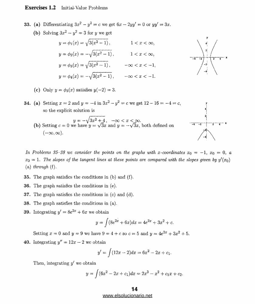
33. (a) Differentiating 3x2 — y2 = c we get 6x — 2yyf = 0 or yy' = 3a;.
(b) Solving 3a:2 — y2 = 3 for y we get
y = ©1 (a:) = \/3{x2 - 1).
y = <h(x) = - \‘3(x- - 1)
y = M x) =
1 < a; < oo,
1 < x < oo.
—oc < x < —1.
—oo < x < —1.y = <?4 (x) = ~\j3{x2 - 1),
(c) Only y = <pz{x) satisfies y{—2) = 3.
34. (a) Setting x = 2 and y = —4 in 3;r2 — y2 = c we get 12 — 16 = —4 = c,
so the explicit solution is
y = —y 3a:2 + 4, —oo < x < oo.(b) Setting c. = 0 we have y = \/3a: and y = — \/3 , both defined on
(—oo;oc).
yi4:
Jn Problems 35-38 we consider the points on the graphs with x-coordinates xq = —1. xq = 0, a
;Z*0 = 1. 77?,e slopes of the tangent lines at these points are compared with the slopes given by y'(xo)
(a) through (f).
35. The graph satisfies the conditions in (b) and (f).
36. The graph satisfies the conditions in (e).
37. The graph satisfies the conditions in (c) and (d).
38. The graph satisfies the conditions in (a).
39. Integrating y' = 8e2x + 6x we obtain
y = j (8e2x’ + Qx)dx = 4e2x + 3x2 + c.Setting x = 0 and y — 9 we have 9 = 4 + c so c = 5 and y — 4e2x -f 3a:2 + 5.
40. Integrating y" — 12x — 2 we obtain
y' = j (12a; - 2)dx = dx2 - 2x + ci.
Then, integrating y! we obtain
y = / (6x2 — 2x + ci)dx = 2x?J — x2 + Cix + oi-
14www.elsolucionario.net

Exercises 1.2 Initial-Value Problems
- 1 the y-coordinate of the point of tangency is y = —1+5 = 4. This gives the initial condition
= 4. The slope of the tangent line at x = 1 is y'(l) = —1. From the initial conditions we
n
6 — 2 + ci = —1 or Ci ~ —5.
. ci = —5 and oi = 8, so y = 2a'3 — x2 — 5ir + 8.
l x = 0 and y = , y' = — 1, so the only plausible solution curve is the one with negative slope
solution is tangent to the .i’-axis at (rro, 0), then y' = 0 when x - xq and y = 0. Substituting
values into y' + 2y = 3x — G we get 0 + 0 = 3-I'q — 6 or :co = 2.
heorcm guarantees a unique (meaning single) solution through any point. Thus, there cannot
o distinct solutions through any point.
2) = ^ (16) = 1. The two different solutions are the same on the interval (0, oo), which is all
h required by Theorem 1.2.1.
= 0. dP/dt = 0.15P(0) + 20 = 0.15(100) + 20 = 35. Thus, the population is increasing at a
.■f 3.500 individuals per year.
population is 500 at time t = T then
2 — 1 + ci + C2 = 4 or ci + c-2 — 3
5 ), or the black curve.
— = 0.15P(r) +*20 = 0.15(500) + 20 = 95. dt t=T
. at this time, the population is increasing at a rate of 9,500 individuals per year.
www.elsolucionario.net

Exercises 1.3 Differential Equations as Mathematical Models
r . ..... ..................................... : . 7 T ' " „ >. r;; ; ;*:* : ;
- Differential Eqti^feioiis
dP dP1. —— — kP + r; — kP — r
dt dt2. Let b be the rate of births and d the rate of deaths. Then b - k]_P and d = k^P- Since dPjdt — b—d,
the differential equation is dP/dt = k\P — k P-
3. Let b be the rate of births and d the rate of deaths. Then b — k\P and d = k^P'2. Since dP/dt = b—d.
the differential equation is dP/dt — kiP — I^P2.
d.P4. —— — h P - k2P 2 -h, h > 0
dt5. From the graph in the text we estimate To = 180° and Tm = 75°. We observe that when T = 85,
dT/dt « — 1. From the differential equation we then have
k = t m _ = ^ i _ = _ 0 1
' T - Tm 85-75
6. By inspecting the graph in the text we take Tm to be Tm(t) = 80 — 30 cos nt/12. Then the
temperature of the body at time t is determined by the differential equation
dT — — k dt
T - 80 - 30 cos5*)] t > 0.
7. The number of students with the flu is x and the number not infected is 1.000 — x, so dx/dt —
fcc(1000 - a:).
8. By analogy, with the differential equation modeling the spread of a disease, we assiune that the rate
at which the technological innovation is adopted is proportional to the number of people who have
adopted the innovation and also to the number of people, y(t), who have not yet adopted it. Then
x + y — n. and assuming that initially one person has adopted the innovation, we have
d r— kx(n — a?), x(0) = 1.
(a*L
9. The rate at which salt is leaving the .tank is
( A \ 4 Rout (3 gal/min) • lb/gal j = — lb/min.
Tims dA/dt = — A/100 (where the minus sign is used since the amount of salt is decreasing. The
initial amount is A(0) = 50.
10. The rate at which salt is entering the tank is
Riu = (3 gal/min) • (2 lb/gal) = 0 lb/min.
16www.elsolucionario.net
Exercises 1.3 Differential Equations as Mathematical Models
Since the solution is pumped out at a slower rate, it is accumulating at the rate of (3 — 2)gal/min
1 gal/min. After t minutes there are 300 + 1 gallons of brine in the tank. The rate at which salt is
leaving is R„t = (2 gal/min) • lb/gal) = ^ - lb/miu.The differential equation is
dA „ 2A = 6
dt 300 + 1
11. The rate at which salt is entering the tank is
R in = (3 gal/min) • (2 lb/gal) = 6 lb/min.
Since the tank loses liquid at the net rate of
3 gal/min — 3.5 gal/min = —0.5 gal/min.
after t minutes the number of gallons of brine in the tank is 300 — \t gallons. Thus the rate at
which salt is leaving is
/ A \ 3 5 4 7/4^ = lb/gal) ' (3'5 gal/min) = soS^tT Slb/min = 6 0 0 ^7 lb/mi,L
The differential equation is
dA „ 7A dA 7
~dt= 600^-i °r M + 600^1 A = 6'
12. The rate at which salt is entering the tank is
R in = {('in lb/gal) • (rin gal/min) = cinrin lb/min.
Xow let A(t) denote the number of pounds of salt and N(t) the number of gallons of brine in the tank
at time t. The concentration of salt in the tank as well as in the outflow is c(t) = x(t)/N(t). But
'he number of gallons of brine in the tank remains steady, is increased, or is decreased depending
:m whether r*n = rQUt, n n > rout. or r.,;n < rou*. In any case, the number of gallons of brine in the
:ank at time t is N(t) = Nq + (r?:n — rout)i. The output rate of salt is then
Rout = ( v , , A---- rr lb/gal J • (rout gal/min) = rmt A---- - lb/min.+ (nn - rout)t J M + (rin - rout)t
The differential equation for the amount of salt,-dA/dt = Rin — R0Uf, is
dA A dA Tout ,i, — (%nr in r out . r . , _ o r ,, + AT , A — ^HnXin
dt A q H- yTin Tovt/t d t A q i [Tin Touf ) t
The volume of water in the tank at time t is V = Awh. The differential equation is then
d,h _ 1 dV _ 1 / \ cAft fV 2 g h .
17www.elsolucionario.net
Exercises 1.3 Differential Equations as Mathematical Models
{ 2 \ ~ 7rUsing Aft = 7T ( —— ) — — , Aw = 102 = 100, and g = 32. this becomes
12J 36
dt 100 450
14. The volume of water in the tank at time t is V = ^wr2h where r is the radius of the tank at hcig;.'
h. Prom the figure in the text we see that r/'h - 8/20 so that r = ‘lh and V = |tt (jJ i) h =
Differentiating with respect to t, we have dVjdt = ^ n h 2 dh/dt or
dh 25 dV
dt A-nh2 dt
From Problem 13 wc have dV/dt = —cA}ly/2gh where c = 0.6, .4/,. = tt , and g = 32. Thu-
dV/dt = — 2tt\//i/15 and
dh _ _25_ ( 2tr\/h.\ _____ 5 _
dt 4tt/j2 y 15 ) 6/i3/2
15. Since i = dq/dt and Ld2q/d,t2 + Rdq/dt = E(t), we obtain Ldi/dt + Ri = E(t).
16. By KirchhofFs second law we obtain R ^ + ~q = E(t).
do *17. From Newton’s second law we obtain m— - —kv2 + mg.dt
18. Sincc the barrel in Figure 1.3.16(b) in the text is submerged an additional y feet below its equilibrium
position the number of cubic feet in the additional submerged portion is the volume of the circular
cylinder: 7rx (radius)2 x height or ix{s/2)2y. Then we have from Archimedes’ principle
upward force of water on barrel = weight of water displaced
= (62.4) x (volume of water displaced)
= (62.4)-7r(6'/2)2jt/ = 15.67rs2y.
It then follows from Newton’s second law that
w d2u , „ „ o d2y 15.67r,s2o- - f = —15.67TS y or - £ + ----- £ y = 0,g dt1 dtr w
where g = 32 and w is the weight of the barrel in pounds.
19. The net force acting on the mass is
_ (f2x , .F = ma = m = —k{s + x) + mg = —kx + mg — ks.
Since the condition of equilibrium is mg - ks, the differential equation is
c£2x
m d P = ~kX'
18www.elsolucionario.net
Exercises 1.3 Differential Equations as Mathematical Models
20. From Problem 19. without a damping force, the differential equation is rnd2x/dt2 = —kx. With a
damping force proportional to velocity, the differential equation becomes
d2x , ,.dx rn —7T = —kx — p—
dt2 ’ dt
d2x Axo r m ~37> + f t — + k'x = 0 .
dt/ dt
21. From g — k/R2 we find k = gli2. Using a = d2r/d,t2 and the fact that the positive direction is
upward wc get
gR2i 1 f ----------- —I— ----
r2
kc f r = _ ___
dt2 a r2
d2r gR?or *5+1 =a22. The gravitational force on m is F = —kMrm /r2. Since Mr = 4irSr^/3 and M = 47r5i ?3/3 wc have
Mr = i:iM j R3 and
F = -kMrm
= - k = -km.M
Now from F = rria = d?7'/dt2 we have
d-r , rnM d~rm —w = —k ——r- r or —=•
dt2 R* dt2
dA
R *
kM
r .
r .
23. The differential equation is —- = k(M — A).dtdA
24. The differential equation is = ki(M — A) — k^A.dt
25. The differential equation is x'(t) = r — kx(t) whore k > 0.
26. By the Pvthagorcan Theorem the slope of the tangent line is y — ,—
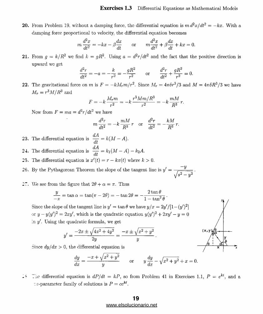
27. We see from the figure that 29 + a = tt. Thus
V 2 tan 9—- = tan a = tan(7r — 29) = — tan 2$ = ------ .-x v ; 1 — tan2 9
Sincc the slope of the tangent line is ?/ - tan 0 we have y/x = 2y'/[l — {yr)2]
or y — y(y')‘2 = 2xy', which is the quadratic equation y(y')'2 + 2xy' — y — i)
in y'. Using the quadratic formula, we get
f —2x± ^4x2 + 4y2 —x ± ijx2 + y2
V 2 y y
Since dy/dx > 0, the differential equation is
dy _ -x + ^x 2 + y2
dx yor
dy
dx
.lie differential equation is dP/dt = kP, so from Problem 41 in Exercises 1.1, P ~ eki, and a
e-paramcter family of solutions is P = cekt.
19www.elsolucionario.net
Exercises 1.3 Differential Equations as Mathematical Models
29. The differential equation in (3) is dT/dt = k(T — Tm). When the body is cooling, T > Tm, so
F Tm > 0. Since T is decreasing, dT/dt < 0 and k < 0. When the body is warming. T <Tm. so
T — Tm < 0. Since T is increasing. dT/dt > 0 and k < 0.
30. The differential equation in (8) is dA/dt — 6 — .4/100. If A(t) attains a maximum, then dA/dt = 0
at this time and A — 600. If A(t) continues to increase without reaching a maximum, then A'{t) > 0
for t > 0 and A cannot exceed 600. In this case, if A'(i) approaches 0 as t increases to infinity, we
see that A(t) approaches 600 as t increases to infinity.
31. This differential equation could describe a population that undergoes periodic fluctuations.
32. (a) As shown in Figure 1.3.22(b) in the text, the resultant of the reaction force of magnitude F
and the weight of magnitude mg of the particle is the ccntripctal force of magnitude muJ2x.
The centripetal force points to the center of the circle of radius x on which the particle rotates
about the y-axis. Comparing parts of similar triangles gives
33. Frorn Problem 21, d~r/dt2 — —gR?/r2. Since R is a constant, if r = R + s, then d?r/dt? = d2s/dt?
and, using a Taylor series, we get
Thus, for R much larger than s, the differential equation is approximated by cPs/dt2 = —g.
34. (a) If p is the mass density of the raindrop, then m — pV and
If dr/dt, is a constant, then dm/dt = kS where pdr/dt = k or dr/dt = k/p. Since the radius is
decreasing, k < 0. Solving dr/dt — k/p we get r = (k/p)t + co- Since r(0) = ro, co — and
r = kt/p + ro.
F cos 9 — mg and F sin 6 = moj2x.
(b) Using the equations in part (a) we find
muj2x u>2x
mg g
(b) From Newton’s sccond law. -r[rmi\ = mg, where v is the velocity of the raindrop. ThenLL'L
dv dm rn — + v —— ~ mg or
dt dt
Dividing by 4p7rr3/3 we get
dv 3 k dv | 3k/p
www.elsolucionario.net
Exercises 1.3 Differential Equations as Mathematical Models
35. We assume that the plow clears snow at a constant rate of k cubic miles per hour. Let t be the
time in hours after noon, x(t) the depth in miles of the snow at time t, and y(t) the distance the
plow has moved in t hours. Then dy/dt is the velocity of the plow and the assumption gives
dy . w x - = k,
where w is the width of the plow. Each side of this equation simply represents the volume of anow
plowed in one hour. Now let to be the number of hours before noon when it started snowing and
let s be the constant rate in miles per hour at which x increases. Then for t > —to, x = s(t + to).
The differential equation then becomes
dy _ k 1
dt ws t + to
Integrating, we obtain
y = — [ln(t + io) + c]ws
where c is a constant. Now when i = 0,y = 0 so c= — Into and
y = i- ln ( l + f ) .W S \ t o J
Finally, from the fact that when t — 1, y = 2 and when t = 2, y = 3, we obtain
2 \ 2IV
1 + t0) V1 + t0J
Expanding and simplifying gives tg + to — 1 = 0. Since to > 0. we find to ~ 0.618 hours
37 minutes. Thus it started snowing at about 11:23 in the morning.
36. (1): = kP is linear dt
dT(3): — = k(T - Tm) is linear
j y
(6): = k(a — X)(,3 — X) is nonlinear dt
(10): y/2gh is nonlinear
(12): = —g is linear
d?s . ds . ..(15): m-rrr + k— = mq is linear
' dt2 dt
(16): linearity or nonlinearity is determined by the manner in which W and T\ involve x.
A-h
dA(2): — = kA is linear
dt
dx(•5): — = kx(n + 1 — a;) is nonlinear
dt
d A „ A . ,
(8): l i = 6 “ Too 18 Unear
I11): + R 'j-t + ,'1 = E(t) is linear
dv(14): m,—~ = mg — kv is linear
dt
21www.elsolucionario.net

Chapter 1 in Review
Chapter 1 in Review . * „t tr. -litJ? Si ..': ~!:v ‘ vf r \:: .........*r”‘' c .........• r “• “ •“ ,7 5' r‘ j :v. .*» . ;f/
1. 4- ci el0x = 10cie10x: ^ = 10ydx ax
2. -y-(5 + cie~2x) = —2cie~2x = —2(5 + cie_2;C — 5); ^ = -2{y - 5) or ^ = -2y + 10 dx ax ax
3. — (c\ cos 4- C2 sin A:.X') = — A;ci sin fcr + fcc? cos kx: dx
d2 9(ci cos fcrc + C2 sin kx) = —k2c\ cos kx — fc2C2 sin fcx = —k?{c\ cos kx + 0 2 sin kx);
dx2
d2y ,2 d%lJ , ,2 n* 3 = - ^ or 5 ? + A:!' = 0d
4. — (ci cosh A~;r + co sinh kx) ~ kci sinh kx + kca cosh kx: dx
d2(ci cosh fcc + C2 sinh kx) = k2c\ cosh kx + k2c:-2 sinh kx = k2{c\ cosh kx + C2 sinh kx);
dx2
^ = k2y 01 ^ ~ k2y=05. y = c\ex + C2 xex; y' — c\ex + C2 xex + C2 ex; y" = c\ex + C2 xex + 2c2(?;
y" + y = 2(ciex + C2 xex) + 2c2ex = 2(ciex + C2 xex + C2 ex) = 2 y'; y" — 2yr + y = 0
6. y' — —c\ex sin x + c\ex cos x + C2 &x cos x 4- C2 CX sin x;
y" = — c\ex cos x — c\ex sinx — c\ex sin x + c\ex cos x — &2 (tx sin x 4- C2 &x cos x 4- C2 ex cos x + C2 ex sin
= —2ciex sin x + 2 c2 ex cos x:
y" — 2y' — —2ciex oosx — 2 c2 ex sinx = —2y; y” — 2y' + 2y = 0
7. a,d 8. c 9. b 10. a,c 11. b 12. a,b;d
13. A few solutions are y = 0, y = c, and y = e1'.
14. Easy solutions to see are y = 0 and y = 3.
15. The slope of the tangent line at (x. y) is y'. so the differential equation is tj — x2 + y2.
16. The rate at which the slope changes is dy'fdx — y", so the differential equation is y" = —y' c
y” 4- y' = 0.
17. (a) The domain is all real numbers.
(b) Since y' = 2j'ix1 . the solution y = x2 is undefined at x — 0. This function is a solution ■
the differential equation on (—oo,0) and also on (0, oo).
22www.elsolucionario.net
Chapter 1 in Review
IS. (a) Differentiating y2 — 2y = x2 — x + c we obtain 2yy' — 2y' = 2x — I or (2y — 2)y' = 2x — 1.
(b) Setting :r = 0 and y = 1 in the solution wc have 1 — 2 = 0 — 0 + corc = —1. Thus, a solution
of the initial-value problem is y2 — 2y = x2 — x — 1.
(c) Solving y2—2y— (x2—x—1) = 0 by the quadratic formula we get y = (2±^/4 + 4(.x2 — x — 1) )/2
= 1 ± V:r2 — x = 1 ± \Jx(x — 1). Since x(x — 1) > 0 for x < 0 or x > 1, we see that neither
y = 1+ \Jx(x — 1) nor y = 1 — ^x(x — 1) is differentiable at x = 0. Thus, both functions are
solutions of the differential equation, but neither is a solution of the initial-value problem.
1?. Setting x = a?o and y = 1 in y = —2/x + x, we get
2 -
Z1
1 = -----------h X0X Q
or Xq - ;ro - 2 = (x-0 - 2)(xq + 1) = 0.
Thus, xq = 2 or xq = —1. Sincc x = 0 in y = —2/x + x. we see that y = —2jx + x is a solution of
■he initial-value problem xy' + y = 2x, y(—1) = 1. on the interval (—oo. 0) and y - —2/x + x is a
? jlution of the initial-value problem xy' + y = 2x. y(2) = 1. on the interval (0, oc).
From the differential equation. y'( 1) = l 2 + [y(l )]2 = 1 + (—l )2 = 2 > 0, so y(x) is increasing in
;:me neighborhood of x = 1. From y" = 2x + 2yy' we have y"( 1) = 2(1) + 2(—1)(2) = — 2 < 0, so
.. .r) is concave down in some neighborhood of x = 1.
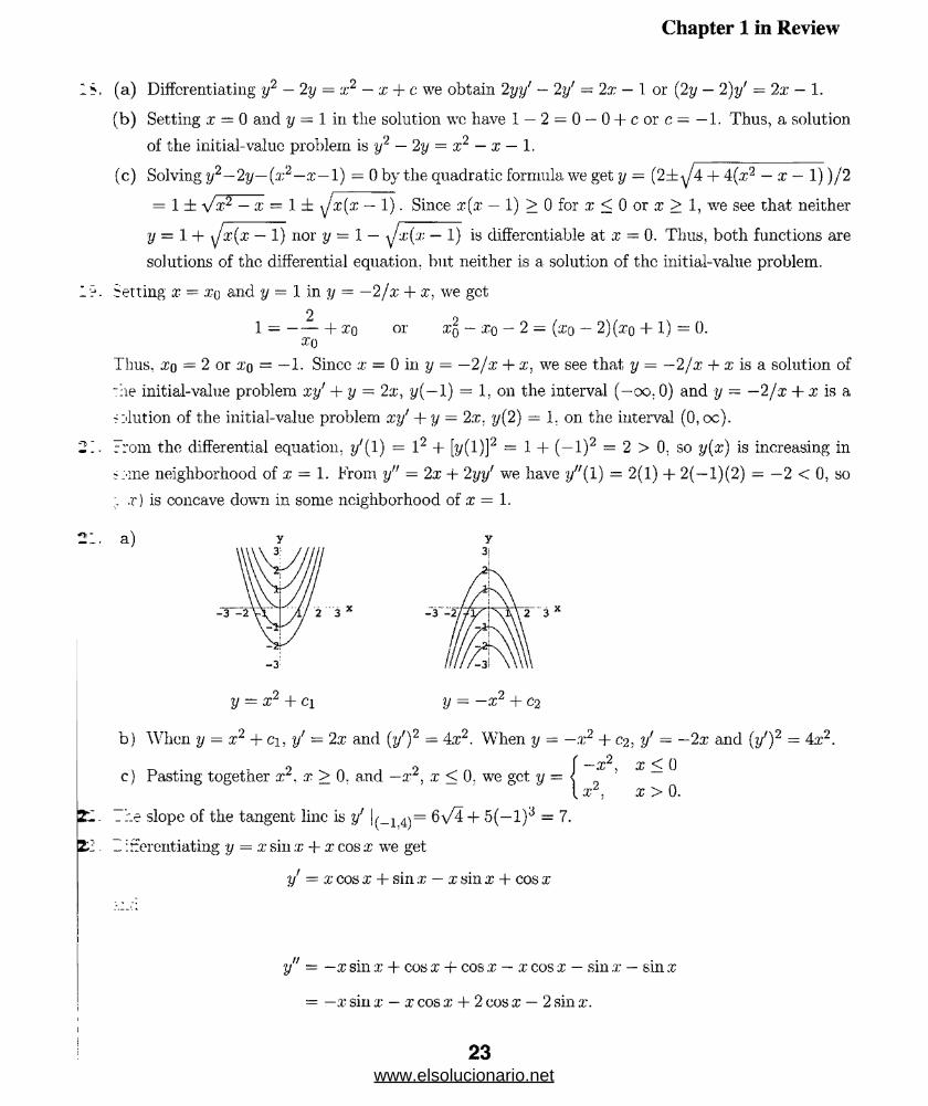
a)
2 3
y — X i j r Cl y = -x2 + C2
b) When y = x2 + ci, y’ = 2x and (y')2 = 4x2. When y = —x2 + C2, y' - —2x and (y')2 = 4.x2.
oc 0 2' ’ ~
x > 0.
_ he slope of the tangent line is y! !(_L4)= 6\/4 + 5(—l)a = 7.
I ifferentiating y = x sin x + x cos x we get
y = x cos x 4- sin x — x sin x + cos x
y = —x sin x + cos x + cos x — x cos x — sin x — sin x
= —x sin x — x cos x + 2 cos x — 2 sin x.
23www.elsolucionario.net

Chapter 1 in Review
Thus
y" + V = ~x sin x — x cos x + 2 cos x — 2 sin x + x sin x + x cos x = 2 cos x — 2 sin x.
An interval of definition for the solution is (—oo, oc).
24. Differentiating y — x sin x + (cos x) In (cos x) we get
/ • / —sina:\ , . X1 / ,y = x cos x + sm x + cos x ---- — (sin x) In (cos x)
\ cos a: /
= x cos x + sin x — sin x — (sin x) ln(cos x)
= x cos x — (sin a:) ln(cos.,r)
and
y" = —.xsinx + cosx — sin;r ( —SmX ) — (cosx) ln(cos.r)V cos a; /
sin2 x= —x sin x + cos x H----— — (cos x) ln(cos x)
cos X
1 — COS2 x= —xsin:r + cos a: H---- ■ — (cosx) ln(cosa:)
cos x
= —x sin x + cos x + sec x — cos x — (cos a;) ln(cos a;)
= —x sin x + sec x — (cos x) ln(cos x).
Thus
y" + y = —x sin x + sec x — (cos ,r) ln(cos a;) + x sin x + (cos x) ln(cos x) — sec x.
To obtain an interval of definition we note that the domain of In a; is (0,oc). so we must hart
cos a; > 0. Thus, an interval of definition is (—tt/2, tt/ 2 ) .
25. Differentiating y — sin (In a:) we obtain y' ~ cos(lna;)/a: and y" = — !sin(lna;) + cos(lna:)]/a;2. Thei:
o if , o f sin(ln x) + cos(ln x) \ cos (In x) . x y + xy' + y = x2 ( --- --- -------- - J + x --K-— - + sin (In a;) = 0.
An interval of definition for the solution is (0, oo).
26. Differentiating y = cos(ln x) ln(cos(ln a:)) + (In x) sin(ln x) we obtain
, , 1 ( sin(ln.r)\ / sin(lna;)\ cos(lna;) sin(ln.r)y' = cosfln a;)— -— r --- --- - + ln(cos(ln.x))--- i + In a:— -- - H--- -- -
cos (In a;) \ x J \ " 'a; x x
ln(cos(lna;)) sin(lna;) (lnx) cos(hi.x)
a;
24www.elsolucionario.net

Chapter 1 in Review
and
y" = -x. . . .005(111:/;) . . 1 / sm(lna;)\In (cos (In re))-- --- - + sin(hi;r)-- -— -(--- --- -
x cosllna;)' x ' x-2
+ In (cos (In a')) sin (In a:)—x + xx-
(In (
(In x)
sin(In x) \ cos (In x)
x x— (lna:) cos (In x)
x
„,2sin2 (In x)
■ ln(cos(ln a;)) cos(ln ar) H--- — - + ln(cos(lna;)) sin(ln j :)cos (In x)
— (lna;) siii(ln;r) + cos(ln:r;) — (lna;) cos(lna:)
Then
x2y" + xy' + y = — In (cos (In x)) cos (lna;)sin2 (In a;)
+ ln(cos(lna;)) sin (In x) — (lna;) sin (In ;r)cos(lna;)
f cos (In x) — (In x) cos (In x) — ln(cos(ln a;)) sin (In x)
+ (In x) cos(ln x) + cos(ln x) ln(cos(ln x)) + (In x) sin (In x)
1sin2(In#) . sin2(Inx) -f cos2(Ina:)v ’ +cos(lna;) = — v v ’ = sec (In a;).
cos (In a;) ' cos(lna:) cos(lnu;)
To obtain an interval of definition, we note that the domain of lna; is (0.oo), so we must have
:os(lna;) > 0. Since cos a; > 0 when —7r/2 < x < tt/2, we require —tt/2 < lna: < tt/2. Since ex
an increasing function, this is equivalent to e_,r/2 < x < e*^1. Thus, an interval of definition is
,,-71/2 _e?r/2). (Much of this problem is more easily done using a computer algebra system such as
'.lathematica or Maple.)
p-oblems 27 ~ 30 we have y' ~ 3c\(?x — 0 2.e~x — 2.
The initial conditions imply
ci + c2 = 0
3 c i - C2 - 2 = 0 ,
-a c i
The initial conditions imply
Cl + C2 = 1
3 c i — C2 — 2 = —3,
- j ci = 0 and C2 = 1. Thus y = e~x — 2x.
25www.elsolucionario.net

Chapter 1 in Review
29. The initial conditions imply
3cie‘5 — C2e-i — 2 = —2,
cie3 + C2e 1 — 2 = 4
so ci = §e 3 and C2 - f e. Thus y = |e3a' 3 + f e X+1 — 2a;.
30. The initial conditions imply
c ie -3 + C26 + 2 = 0
3cie-3 — c-2e — 2 = 1,
so ci - |e3 and ox = — |e_1. Thus y = ie3-TK? — \e~x~l — 2,t.
31. From the graph we see that estimates for yo and yi are yo : —3 and yi = 0.
32. The differential equation isdh cAq
y f c h .dt Aw
Using Ao = 7r(l/24)2 = 7r/576, Aw = tt(2)2 = 4tt, and g — 32, this becomcs
^ = _ £ ^ 0 v ® ; =(it 4tt 288
33. Let F(t) be the number of owls present at time t. Then dP/dt = k(P — 200 + lOt).
34. Setting A7(i) = —0.002 and solving A'(t) = —0.0004332A(£) for A(t), we obtain
A ' ( f ) - ° - 002
‘ “ -0.0004332 ~ -0.0004332 ~ ' gramS'
26www.elsolucionario.net
2 First-Order Differential Equations
27
www.elsolucionario.net
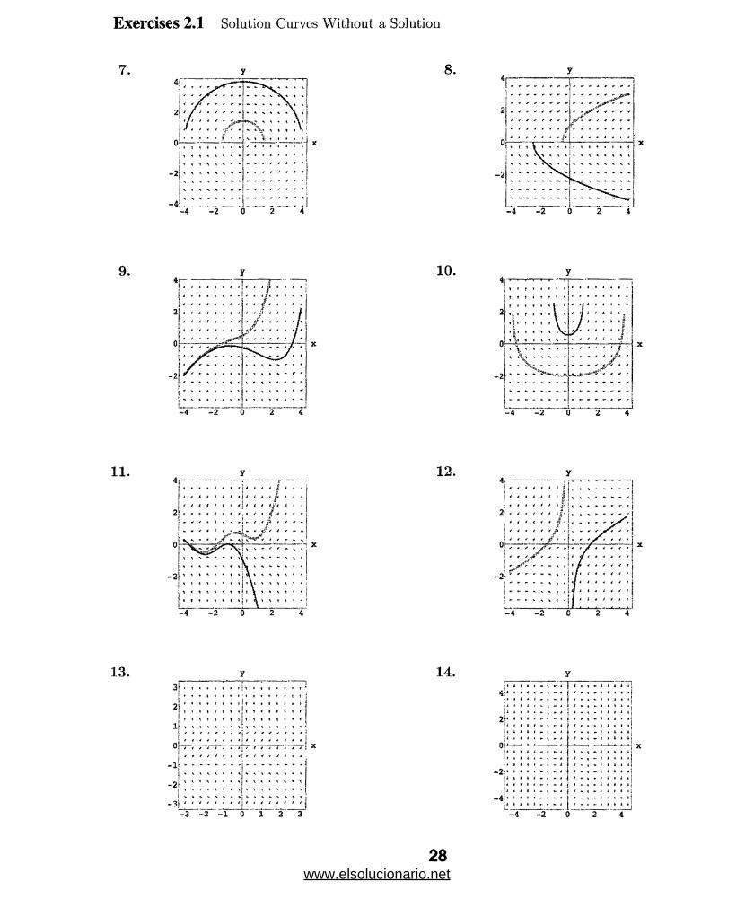
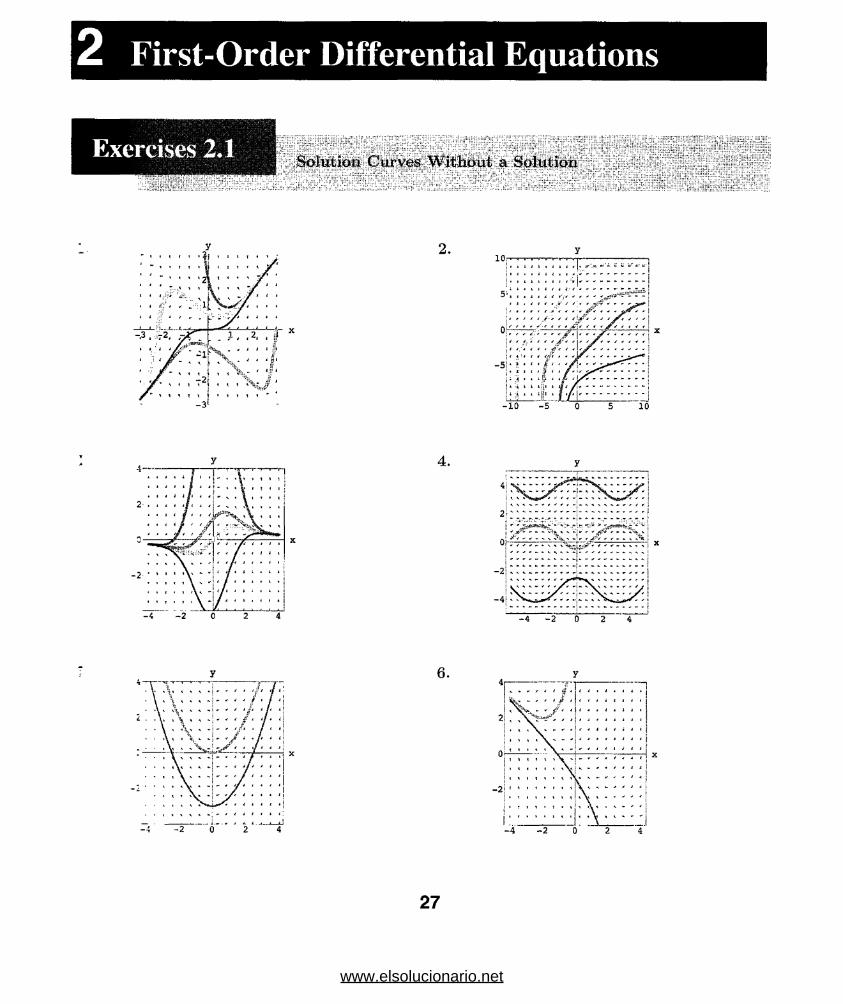
Exercises 2.1 Solution Curves Without a Solution
28www.elsolucionario.net
Exercises 2.1 Solution Curves Without a Solution
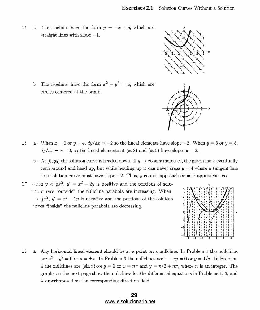
i. he isoclines have the form y = —x + c. which are
straight lines with slope —1.
The isoclines have the form x2 + y2 = c. which are
circles centered at the origin.
I" a 1 When x = 0 or y = 4, dy/dx = —2 so the lineal elements have slope —2. When y — 3 or y = 5,
dy/dx = x — 2. so the lineal elements at (x, 3) and (x, 5) have slopes x — 2.
b ■ At (0, yo) the solution curve is headed down. If y —> oo as x increases, the graph must eventually
turn around and head up, but while heading up it can never cross y = 4 where a tangent line
to a solution curve must have slope —2. Thus, y cannot approach oo as x approaches oo.
1" "'.".'.on y < \x2, y' = x2 — 2y is positive and the portions of solu-
curves “outside” the nullcline parabola are increasing. When
> jx 2, y' = x2 — 2y is negative and the portions of the solution
::-ves "inside” the nullcline parabola arc decreasing.
-3-2-10 1 2 3
a ) Any horizontal lineal element should be at a point on a nullcline. In Problem 1 the nullclincs
are x2 — y1 — 0 or y — ±x. In Problem 3 the nullclines are 1 — xy = 0 or y — l/x. In Problem
4 the nullclines are (sina;) cosy ■ 0 or x - rwr and y — 7r/2 + rm, where n is an integer. The
graphs on the next page show the nullclines for the differential equations in Problems 1,3, and
4 superimposed on the corresponding direction field.
y
29www.elsolucionario.net
Exercises 2.1 Solution Curves Without a Solution
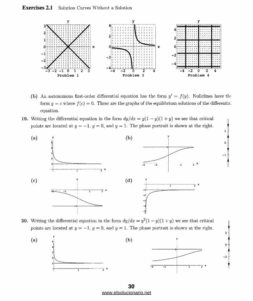
(b) An autonomous first-order differential equation has the form y' = f(y). Nullclines have tli-
form y = c where /(c) = 0. These are the graphs of the equilibrium solutions of the differentia
equation.
19. Writing the differential equation in the form dy/dx = y(l — y)(l + y) we see that critical
points arc located at y = — 1, y = 0, and y — 1. The phase portrait is shown at the right.
(a) (b)
(c) (d)
20. Writing the differential equation in the form dy/dx = y2(l — y)(l + y) we see that critical
points are located at y = — 1. y — 0, and y = 1. The phase portrait is shown at the right.
(a) (b)
- i
o--
30www.elsolucionario.net

Exercises 2.1 Solution Curves Without a. Solution
ic) (d)
Solving y2 — ‘3y = y(y — 3) = 0 we obtain the critical points 0 and 3. From the phase
portrait we see that 0 is asymptotically stable (attractor) and 3 is unstable (repeller).
jiving y2 - yz = y2(l — y) = 0 we obtain the critical points 0 and 1. From the phase
jrtrait we see that 1 is asymptotically stable (attractor) and 0 is semi-stable.
: jiving (y — 2)4 = 0 we obtain the critical point 2. From the phase portrait we see that
is semi-stable.
' jiving 10 + 3y — y2 = (5 — y)(2 + y) — 0 we obtain the critical points —2 and 5. From
::.e phase portrait we see that 5 is asymptotically stable (attractor) and —2 is unstable v
:\'-peller). s--
A
31www.elsolucionario.net
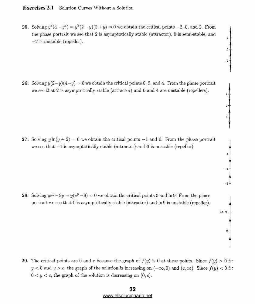
25. Solving y1{ 1 — if) = y2( 2 — y)(2 + y) = 0 we obtain the critical points —2, 0, and 2. From I
the phase portrait we see that 2 is asymptotically stable (attractor), 0 is semi-stable, and
—2 is unstable (rcpeller).
o
- 2 -
26. Solving y { 2 —y ) ( 4 — y ) = 0 we obtain the critical points 0, 2. and 4. From the phase portrait
we see that 2 is asymptotically stable (attractor) and 0 and 4 are unstable (repellers). a4 ~ -
2 - -
A0
V
27. Solving yln(y -f 2) = 0 we obtain the critical points —1 and 0. From the phase portrait
we see that —1 is asymptotically stable (attractor) and 0 is unstable (repeller). a
o-
u
- i ■
A
-2 -
28* Solving yey — 9y = y(eJJ — 9) = 0 we obtain the critical points 0 and In 9. From the phase
portrait we see that 0 is asymptotically stable (attractor) and In 9 is unstable (repeller). a
In 9 -
u
0
A
29. The critical points are 0 and c because the graph of f(y) is 0 at these points. Since f(y) > 0 ft:
y < 0 and y > c, the graph of the solution is increasing on (—oo,0) and (c, oc). Since f(y) < 0 fc:
0 < y < c. the graph of the solution is decreasing on (0, c).
Exercises 2.1 Solution Curves Without a Solution
32www.elsolucionario.net

Exercises 2.1 Solution Curves Without a Solution
:e critical points are approximately at —2,2. 0.5, and 1.7. Since f(y) > 0 for y < —2.2 and
: < y < 1.7, the graph of the solution is increasing on (—oc, —2.2) and (0.5,1.7). Since f(y) < 0
: —2.2 < y < 0.5 and y > 1.7, the graph is decreasing on (—2.2,0.5) and (1.7, oc).
y
1.7
0.5
- 2 . 2
. :r, the graphs of 2 = t t / 2 and z — sin y we see that
2 y — sm y = 0 has only three solutions. By inspection
're that the critical points are —t t / 2 . 0, and t t / 2 .
:::: the graph at the right we see that
2 f < 0 fo r y < —tt/ 2— y — s in y <7T \ > 0 fo r y > t t / 2
2 f > 0 for— — sm y <7T I < 0 for
r/2 < y < 0
0 < y < 7r/2.
o --
. _> -nables us to construct the phase portrait shown at the right. From this portrait we see that
• 1 :.::d — 7r/2 are unstable (repellers), and 0 is asymptotically stable (attractor).
dx = 0 every real number is a critical point, and hence all critical points are nonisolated.
that for d y / d x = f ( y ) we are assuming that / and f are continuous functions of y on
33www.elsolucionario.net
Exercises 2.1 Solution Curves Without a Solution.
some interval I. Now suppose that the graph of a nouconstant solution of the differential equation
crosses the line y = c. If the point of intersection is taken as an initial condition we have two distinct
solutions of the initial-value problem. This violates uniqueness, so the graph of any nonconstant
solution must lie entirely on one side of any equilibrium solution. Since / is continuous it can only
change signs at a point where it is 0. But this is a critical point. Thus, f(y) is completely positive
or completely negative in each region Rt. If y(x) is oscillatory or has a relative extremum, then
it must have a horizontal tangent line at some point (xo, yo)- In this case yo would be a critical
point of the differential equation, but we saw above that the graph of a nonconstant solution canno:
intersect the graph of the equilibrium solution y = yo-
34. By Problem 33, a solution y(x) of dy/dx = f(y) cannot have relative extrema and hence must b-r
monotone. Sincc y'{x) = f(y) > 0, y(x) is monotone increasing, and since y(x) is bounded abo\v
by C2; lim:E_>0o y{x) — L. where L < 0 2 ■ We want to show that L = c-2 . Since L is a horizonta.
asymptote of y(x), lim3._»0c y!(x) — 0. Using the fact that f(y) is continuous we have
f(L) = f Q ^ v ( x)) = J™ c/(y(^)) = = °-
But then L is a critical point of /. Since ci < L < C2, and / has no critical points between ci an..
02, L = 02.
35. Assuming the existence of the second derivative, points of inflection of y(x) occur where-
y"(x) - 0. From dy/dx = f(y) we have d2y/dx2 = f(y ) dy/dx. Thus, the ^-coordinate of
point of inflection can be located by solving f'(y) = 0. (Points where dy/dx = 0 correspond
constant solutions of the differential equation.)
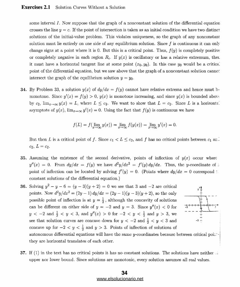
36. Solving y2 — y — 6 = (y — 3)(y + 2) = 0 we see that 3 and —2 arc critical a
points. Now d2y/dx2 = (2y — 1) dy/dx = (2y — l)(y — 3)(y + 2). so the only ______ + ___
possible point of inflection is at y = \ , although the concavity of solutions \f \
can be different on cither side of y = —2 and y = 3. Since y"(x) < 0 for -s1 1 1 11 1 '\1 1 j
y < —2 and | < y < 3, and y"{x) > 0 for —2 < y < ^ and y > 3, we +
see that solution curves are concave down for y < —2 and \ < y < 3 and ~5 - |
concave up for — 2 < y < ^ and y > 3. Points of inflection of solutions of
autonomous differential equations will have the same y-coordinat.es beeausc between critical poi:.' -
they are horizontal translates of each other. !
37. If (1) in the text has no critical points it has no constant solutions. The solutions have neither
upper nor lower bound. Since solutions are monotonic, every solution assumes all real values.
34www.elsolucionario.net

Exercises 2.1 Solution Curves Without a Solution
The critical points are 0 and b/a. From the phase portrait we see that 0 is an attractor
and b/a is a repeller. Thus, if an initial population satisfies Po > b/a, the population
becomes unbounded as t increases, most probably in finite time, i.e. P(t) —► oo as t —> T.
I: 0 < Po < b/a, then the population eventually dies out, that is, P(t) —> 0 as t —► oo.
Since population P > 0 we do not consider the case Pq <0.
The only critical point of the autonomous differential equation is the positive number h/k. A
phase portrait shows that this point is unstable, so h/k is a repeller. For any initial condition
P 0) = Po < h/k.dP/dt < 0; which means P(t) is monotonic decreasing and so the graph of P(t)
:;:ust cross the 2-axis or the line P = 0 at some time t,\ > 0. But. P{t\) = 0 means the population
it extinct at time t,\.
Writing the differential equation in the form
dv k / mg \
dt m V k )
see that a critical point is mg/k. ^
From the phase portrait we see that mg/k is an asymptotically stable criticalit
" I'int. Thus, lim^oc v = mg/k.
■ riting the differential equation in the form
see that the only physically meaningful critical point is y jmg/k.
From the phase portrait we see that yrng/k is an asymptotically stable
:i:ical point. Thus, lim^oc v = yjrng/k.
a) From the phase portrait we see that critical points are a and ,3. Let X(0) = Xq.
If Xo < a, we see that X —> a as t —► oo. If a < X q < /3, we see that X —> a as
t —> oc. If Xq > B, we see that X(t) increases in an unbounded manner, but more
specific behavior of X(t) as t —> co is not known.
[mgV 'k
35www.elsolucionario.net
Exercises 2.1 Solution Curves Without a Solution
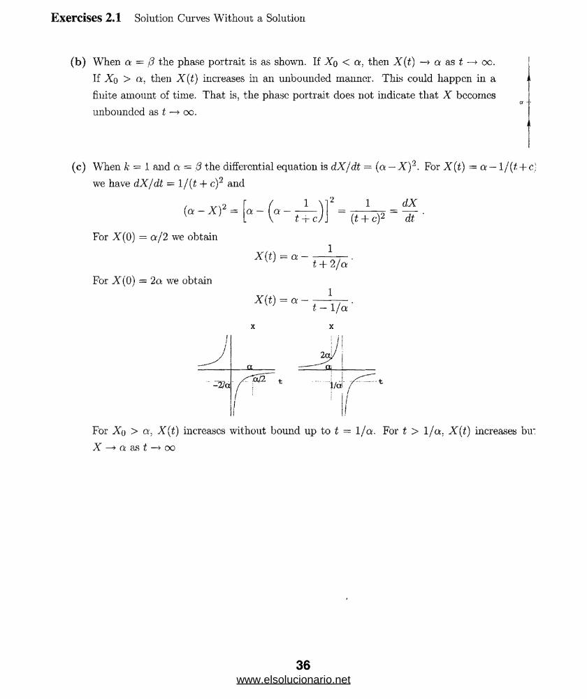
(b) When a = 0 the phase portrait is as shown. If X q < a, then X(t) —»■ a as t —► oc. j
If X q > a, then X(t) increases in an unbounded manner. This could happen in a a
finite amount of time. That is, the phase portrait does not indicate that X becomesa ■■■■
unbounded as t —► oc.
(c) When k = 1 and a = 3 the differential equation is dXf dt = (a — X)'2. For X(t) = a — l/(t + c]
we have dXjdt = l/(t + c)~ and
1 M 2 1 dX(a - X ? =
For X(0) = a/2 we obtain
For A"(0) = 2a we obtain
a — [a —t-rC (t + c)2 dt
X (t) = a —
X(t) = a~
1
t + 2j a
1
t — 1/a ’
xf/j ! fl
: 11 2a|/
a --- a:
!j
... _^a ‘•3.........
.........
i f .....*II
For X q > a, X(t) increases without bound up to t = 1/a. For t > 1/a., X(t) increases bu:
X —► a as t —► oo
36www.elsolucionario.net

Exercises 2.2 Separable Variables
Exercises 2.2Separable Variables
■ v of the following problems we will encov,nter an expression of the form, In j<7(y)| = f(x) + c. To
d(y) we exponentiate both sides of the equation. This yields |<7(y)| = eAx)+c = e,:e / ^ which
- 9iy) — ±ece.f(x\ Letting ci = we obtain g(y) = c\g x\
:; :n dy = sin 5.x dx we obtain y — — | cos 5x + c.
;:m dy = (x + l )2 dx we obtain y ~ j(x -f 1) + c.
: : m dy = —e_3x dx we obtain y = |e-3x + c.
1 J 7 i x • 1 1. m ----—p dy = dx we obtain-----= x + cory = l —{y - 1)2 y - 1 ' x + c
1 4':m - dy = — dx we obtain In \y\ = 4 In I#I + c or y = c\x4.
y %
l i . i: .in —~dy = —2x dx we obtain — - —x2 + c or y — —7;
c.
y* y “ z2 + ci
,':>m e~2ydy = e?xdx we obtain 3e~‘2y + 2(/jX = c.
: jiii yevdy — (e~x + e~'ix dx we obtain yey — eu + e~x + = c.
:: :n (y + 2 + - J dy = x2 hi x dx we obtain 7- + 2y + In |yj = ~r- In jx| — i;r'V V J 2 3 9
1 ; 1 u+ . 2 1: 7 ---TT7> dy — 7---- —77 dx we obtain ----- = ----- h c.
(2y + 3)2 J (4* + 5)2 2j/ + 3 4x + 5
1 1' :m i---dy = ----h— dx or sin ydy = - cos2 x dx = — i ( l + cos2x) dx we obtain
csc y ’ scc^x z
:-os y = — \x — | sin 2x + c or 4 cos y = 2x + sin 2x + ci.
s m 3 'v•C'in 2y dy = --- 17— dx or 2y dy = — tan 3x sec2 3.x dx we obtain y2 — —I sec2 3.x + c.
cos'13.x ' 0
ey —exj in ----- k dy = ------o fix wc obtain — (e,J + 1) = A (ex + 1) + c.
(ev + l Y (ex + 1) 2V
V x 7 1 ( 9\ V2 / o\ 1/2:: „-m--- :— 7777 dy = ------^ dx we obtain 1 + y = (1 + x ) + c.
(1 + y2) (l+.x2)1/2 V } . V }
r: .'in — dS = A'dr we obtain S = cekr.
1 :an n 7 n ^ = ^ we °^ta^L h1 IQ — 70| = kt + c or Q — 70 = ciefct.v>r / U
37www.elsolucionario.net

Exercises 2.2 Separable Variables
17. From p j^ d P — ^ ^ dP = dt we obtain In |P| — In |1 — P\ = t + c so that In
t + c or --- — = ci e(. Solving for P we have P =
1 - P
1 - P 1 b l+ c ie* '
18. From c/Ar = ffe*"1"2 — l) dt we obtain In |Ar| = £ef+2 — e<+2 — t + c or Ar = Cie1
y ~~ 2 :e — 1 / 5 \ / 5 \19. From --- - dy = ---- dx or 1---- - dy = (1 ----- - ) dx we obtain y — 5 In \y + 31 =
y + Z x + 4 V y + 3/ V x + 4/
' z + 4 x 0
x — 5 In |x + 4| + c or I - — j = c\ex y.
20. From dy = ^ dx or ( 1 H-- ■) dy = (l-{---- \ dx we obtain y + 2 In \y — 11 =y — 1 ' x - 3 \ y — l j \ x - 3 Jy- 1 x — 3 \ y - 1
x 4- 5 In Lt — 31 + c or ~ — ^ = c\ec~v.(a: — 3)°
1 ■ _ fx 2 \21. From x dx = j dy we obtain 5 a;2 = sin-1 y + c or y = sin + c i j .
1 1 ex 1 122. From — dy = —---— dx - 7— — r dx we obtain — - tan-1 ex + c or y =
y2 ex + e x (ex)2 + 1 y ' tan 1 ex + c '
23. From - — dx = Adt we obtain tan-1 x = At + c. Using x(tt/A) = 1 we find c = — 3ir/A. The•1 | 1
solution of the initial-value problem is tan-1 x = At — or x = tan ( At —
1 , 1 , 1 / 1 1 \ , 1 / 1 1 \ ,24. From — - ay — —— - dx or - --------- - \ dy = - ---------- dx we obtainy2- l :r2 — 1 2 \y-] y + 1 / 2 Var — 1 x + l j
In (y — 1| — hi |y + 1| = In |a: — lj — In la: + 11 + In c or ^ | = — — — • Using y(2) = 2 we findy i 1 ,X r J-
y — 1 x — 1c = 1. A solution of the initial-value problem is ~ ^ - or y = x.
25. From - dy = -—rj— dx = dx we obtain In \y\ = — i — In |x] = c or xy = cie~1/x. Usingl j J/ \ <!■ iX J »./;
y(—l) = —1 we find c\ ~ e-1. The solution of the initial-value problem is xy = or
y = jx.I26. From --- — dy = dt we olrf.ain —g In |1 — 2y| = t + c or 1 — 2y = c\e~2t. Using y(0) = 5/2 wc fine
i — Zy
c-j = —A. The solution of the initial-value problem is 1 — 2y = —4e-2* or y -- 2e~ 2t + ^ .
27. Separating variables aud integrating we obtain
dx dy . _! . _ j- () and sin x — sm y = c.
V l- X 2 y/l - y2
38www.elsolucionario.net

Exercises 2.2 Separable Variables
Setting x = 0 and y = V3/2 we obtain c — — 7r/3. Thus, an implicit solution of the initial-value
problem is sin-1 x—sin-1 y = — tt/3. Solving for y and using an addition formula from trigonometry,
we get
. 7T x \/3 V 1 — x2(* —i \ r o * ^;y = s m ^ s in x + - j = X cos - + y 1 - x / s in - = - +
—xFrom --- ——77 dy = ------~ dx we obtain
1 + (2y) J 1 + (*2)2
^ tan-1 2y = — tan" 1 :c2 + c or tan-1 2y + tan- 1 x2 = ci. z z
Using y(l) = 0 we find c\ = 7r/4. Thus, an implicit solution of the initial-value problem is
tail-1 2y + tan-1 z2 = tt/4 . Solving for y and using a trigonometric identity we get
2y = tan — tan ;r
1 / 7t _ i 9\y — - tan I — — tan x J
1 tan | — tan(tan-1 x2)
2 1+ tan tan(tan_1 x2)
1 1 — x2
2 1 + x2 '
Separating variables, integrating from 4 to and using t as a dummy variable of integration gives
J 4 y dt Ja
lny( f4 = J4 e~ t2(it
\ny(x) — lny(4) = j e~r dt Ja
Using the initial condition we have
lny(a:) = lny(4) + jf e"f2dt = In 1 + e^'dt = eT^ dt.Thus,
y(x) = eh e 1
9
39www.elsolucionario.net
Exercises 2.2 Separable Variables
30. Separating variables, integrating from —2 to x, and using t as a dummy variable of integration gives
r /‘startsy-2 jr at J-2
—y(t)~1 2 = J sint2dt
y(x)_1 + y(-2)_1 = J ^ m t2d,t
—//(x)-1 = —y(—2)_1 + J sint2dt
y(x)~] = 3 — j ^sint2dt.
Thus
= 3 - J ? 2 sin t2dt ‘
31. (a) The equilibrium solutions y(x) = 2 and y(x) = —2 satisfy the initial conditions y(Q) = 2 and
y(0) - —2, respectively. Setting x = | and y = 1 in y = 2(1 + ce4x)/( 1 — ce4x) wc obtain
1 = 21 + ce
1 — ce1 — ce = 2 + 2ce, —1 = 3 ce, and c = —— .
3e
The solution of the corresponding initial-value problem is
1 _ ! p4 a?-l o _ fi4x— 1
y = 2— A - -r = 2- C1 + 3 + e‘
(b) Separating variables and integrating yields
i In |y — 2| — ^ In |y + 2| + In ci = x4 4
In \y — 2\ — In \y + 2j + In c = 4x
c (y - 2 )In
y + 2y -
= 4.x
= ey + 2
Solving for y we get y = 2(c + e4a:)/(c — e4x). The initial condition y(0) = —2 implies
2(c+ l)/(c — 1) = —2 which yields c = 0 and y(x) = —2. The initial condition y(0) = 2 does
not correspond to a value of c, and it must simply be recognized that y(x) = 2 is a solution or
the initial-value problem. Setting x = | and y — 1 in y = 2(c + e4x)/(c — e4x) leads to c = — 3f.
Thus, a solution of the initial-value problem is
_ 3e + e4^ 3 — e4 x - iy = 2 — ----------— = 2
—3e — e4a: 3 + e4-14;r— 1
40www.elsolucionario.net

Exercises 2.2 Separable Variables
32. Separating variables, wc have
dy dx
y2 - y x
Using partial fractions, wc obtain
dy = hi lar| + c
In Jy — lj — In jy| = In |.?;| + c
Solving for y we get y = 1/(1 — cix). Wc note by inspection that y = 0 is a singular solution of the
differential equation.
(a) Setting x = 0 and y = 1 we have 1 = 1/(1 — 0), which is true for all values of c\. Thus,
solutions passing through (0, 1) are y = 1/(1 — cix).
(b) Setting x = 0 and y = 0 in y = 1/(1 — c\x) we get 0 = 1. Thus, the only solution passing
through (0,0) is y = 0.
(c) Setting x = \ and y = \ we have | = 1/(1 — 5 ci), so c\ — —2 and y — 1/(1 + 2x).
I'd) Setting x = 2 and y = { wc have | = 1/(1 —2ci), so ci = -| and y = \/(l + '^x) = 2/(2 + 3x).
I-;. Singular solutions of dy/dx = xy 1. — y2 are y = — 1 and y = 1. A singular solution of
_|_ Q-x'jdyjdx = y2 is y = 0.
14. Differentiating In (x2 + 10) + csc y = c we get
x2 + 10
x2 + 10 sin y sin y dx
2x 1 cos y dy _
2x sin y dx — (x2 + 10) cos ydy = 0.
iting the differential equation in the form
dy 2x sin2 y
dx (x2 + 10) cosy
see that singular solutions occur when sin2 y = 0, or y = km, where k is an integer.
41www.elsolucionario.net
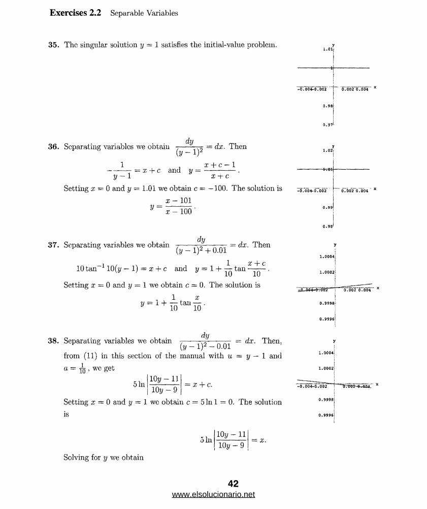
35. The singular solution y = 1 satisfies the initial-value problem.
Exercises 2.2 Separable Variables
y1,0 1
- 0 . 0 0 4 - 0 . 0Q2
0.9 8
0 .0 0 2 0 .0 0 4
36. Separating variables we obtaindy
(V - I )2= dx. Then
1 x + c — 1= x + c and y =
y - 1 x - r e
Setting x = 0 and y = 1.01 we obtain c = —100. The solution is
x - 101y = x — 100
37. Separating variables we obtaindy
{ y - l ) 2 + 0 .0 1= dx. Then
1 x + c10 tan 10(y — 1) = x + c and y = 1 + — tan ^
Setting x = 0 and y — 1 we obtain c = 0. The solution is
v = 1 + i tmTo-38. Separating variables we obtain
dy= dx. Then,
(y - l )2 - 0.01
from (11) in this section of the manual with u = y — 1 and
a = 4 , we get
5 InlOy - 11
= x + c.lOy — 9
Setting x = 0 and y = 1 wc obtain c = 5 In 1 = 0. The solution
is
5 InlOy - 11
lOy - 9= x.
Solving for y we obtain
y1.02?
- 0 . 0 0 4 - 0 . 0 0 2 0 .0 0 2 0 .0 0 4
0 .9 8
1 .0004
1.0002
0.9996?
0 .9 99 6
42www.elsolucionario.net
Exercises 2.2 Separable Variables
l l + ge^ 5
V~ 10 + 10ex/5 '
Alternatively, we can use the fact that
/ (y _ o.oi = -oT “ l lr l IT T = - 10t“ h_110fe - !)•
(We use the inverse hyperbolic tangent becausc \y — lj < 0.1 or 0.9 < y < 1.1. This follows from
the initial condition y(0) = 1.) Solving the above equation for y wc got y — 1 + 0.1 t,anh(x/10).
39. Separating variables, we have
dy = dy (1 _l/2_ _ JV 2_\
y - y 3 i/(i-y)(i+y) \y ' i - y i + y ) v <x'
Integrating, we get1 '1
ln \y\ - 9111 |i - y\ - in |i + y\ = % + c.
When y > 1, this becomes
\n y - J ln(y - 1) - ^ ln(y + 1) = In J?-. = x + c.
2 2 y / y * - 1
Letting x = 0 and y = 2 we find c = ln(2/\/3). Solving for y we get yi (x) = 2c®/V4e2x — 3. where
.r > ln(-\/3/2).
When 0 < y < 1 we have
lny - | ln(l - y) - ^ ln(l. + y) = In ■■ , —.. = :c + c.2 2 V1 - yLetting x = 0 and y = | we find c = ln(l/\/3). Solving for y we get yi{x) — ex/y/e2x + 3, where
—OO < X < oo.
When — 1 < y < 0 we have
In(-V) “ 5 !“ ( !- » ) - 5 l" (l + V) = to , V = x + c.2 2 VT-yLetting x = 0 and y — — \ we find c = ln(l/\/3). Solving for y we get ys(x) = —ex/sj~e2x + 3 ,
where — oc < x < oo.
When y < — 1 wc have
H ~ y ) - \ M 1 - y ) - \ M - 1 - v) = ln , „ y = x + c.2 2 \ / y 2 - 1
43www.elsolucionario.net

Exercises 2.2 Separable Variables
Letting rr = 0 and y — —2 we find c = ln(2/\/3). Solving for y we get Vi(x) = —2ex/y/A.e?x — 3.
where x > ln(\/3/2).
Y
4}iI T " T " 3 4 5
-2]
-41
-4 -2 : 2 4 - 2;
-4
-41
40. (a) The second derivative of y is
d2y dy/dx l/(y — 3)
dx2 ( y - i) 2 (y-3)2 (y-3)3 '
The solution curve is concave down when d2y/dx2 < 0 or
y > 3, and concave up when d2y/dx2 > 0 or y < 3. Prom
the phase portrait wc see that the solution curve is decreasing
when y < 3 and increasing when y > 3.
/"■1 2 3 4 5
(b) Separating variables and integrating we obtain
(y — 3) dy — dx
2 V~ ~ 3V = x + c
y2 - 6y + 9 = 2x + c\
(y ~ 3)" = 2x + ci
y = 3 ± y/2x + c i.
The initial condition dictates whether to use the plus or minus sign.
When yi (0) = 4 we have c\ = 1 and y\(ar) = 3 4- y/2x + 1.
When j/2(0) = 2 wc have ci = 1 and 2/2 (s) — 3 — \/2x + 1 .
When 1/3(1) = 2 we have cj = — 1 and yz(x) = 3 — y/2x — 1 .
When y±(—1) = 4 we have c\ = 3 and 2/4(x) = 3 + y/2x + 3.
41. (a) Separating variables we have 2ydy = (2x + 1 )dx. Integrating gives y2 = x2 + x + c. Whci.
y(—2) -- —1 we find c — — 1. so y2 = x2 + x — 1 and y = —\/x2 + x - l . The negative squar-.
root is chosen because of the initial condition.
44www.elsolucionario.net

Exercises 2.2 Separable Variables
(b) From the figure, the largest interval of definition appears to be y
approximately (—oc. —1.65).2
(c) Solving x2 + x — 1 = 0 we get x = — | ± |\/5, so the largest interval of definition is
(—oo, — | — g\/5)- The right-hand endpoint of the interval is excluded becausc y =
~Vx2 + x — 1 is not differentiable at this point.
(a) From Problem 7 the general solution is Se~2y + 2e3x = c. When y(0) = 0 we find c = 5. so
Se~2y + 2e3x = 5. Solving for y we get y = In ^(5 — 2e3x).
(b) The interval of definition appears to be approximately (—oc,0.3). y2
- 2_
-1
-2
(c) Solving 5(5 — 2e3x) = 0 we get x = g ln(|), so the exact interval of definition is (—00, | In §).
;3. (a) While 1 1 2 (3:') = — \/25 — x2 is defined at x = — 5 and x = 5, y^x) is not defined at these values,
and so the interval of definition is the open interval (—5,5).
(b) At any point on the z-axis the derivative of y(x) is undefined, so no solution curve can cross
the .x-axis. Since —x/y is not defined when y = 0, the initial-value problem has no solution.
=4. (a) Separating variables and integrating we obtain x2 —y2 = c. For c ^ 0 the graph is a hyperbola
centered at the origin. All four initial conditions imply c = 0 and y = ±.r. Since the differential
equation is not defined for y = 0, solutions are y — ±x, x < 0 and y = ±x, x > 0. The solution
for y(a) = a is y = x. x > 0; for y(a) — —a is y = —x; for y(—a) = a is y = —x. x < 0; and for
y(—a) = —a is y = x, x < 0.
(b) Since x/y is not. defined when y = 0, the initial-value problem has 110 solution.
(c) Setting x = 1 and y — 2 in x2 — y2 = c we get c = —3, so y2 = x2 + 3 and y(x) = Vx2 + 3,
where the positive square root is chosen because of the initial condition. The domain is all real
numbers since x2 + 3 > 0 for all x.
45www.elsolucionario.net

Exercises 2.2 Separable Variables
45. Separating variables we have dy/{\j\ + y2 sin2 y) = dx which
is not readily integrated (even by a CAS). We note that
dy/dx > 0 for all values of x and y and that dy/dx = 0
when y = 0 and y — tt: which are equilibrium solutions.
46. Separating variables we have dy/ (y/y+y) = dx/(y/x+x). To integrate f dx/ (y/x + x) we substitute
u? = x and get
/ 2u f 2 --- ~~2 du = / ----du = 2 hi 11 -i- u| + c = 2 ln(l + yfx) + c.
(it | ’ (/- J 1 1
Integrating the separated differential equation we have
2 ln(l + y/y) = 2 ln(l + y/x) + c or ln(l + y/y) ‘ ln(l + ) + In c\.
Solving for y we get y = [ci(l + y/x-) — l]2.
47. We are looking for a function y(x) such that
Using the positive square root gives
dy_
dx
dy= dx sin 1 y = x + c.
\/l - v 2
Thus a solution is y = sin(;c + c). If we use the negative square root we obtain
y = sin(c — x) = — sin (2; — c) = — sin(.x + ci).
Note that when c: — e.\ — 0 and when c = cj = 7t/2 we obtain the well known particular solutionI
y = sin a-, y = — sin®, y = cosx, and y = — cosx. Note also that y — 1 and y = — 1 are singuis
solutions.
46www.elsolucionario.net
Exercises 2.2 Separable Variables
(b) For |a;| > 1 and |yj > 1 tlie differential equation is dy/dx = y'y2 — 1 /■y/x1 — 1. Separating
variables and integrating, we obtain
dy dx , , _i , _i... = , = and cosh y = cosh x + c.
Setting x = 2 and y = 2 wc find c ■ cosh-1 2 — cosh-12 = 0 and cosh-1 y = cosh-1 x. An
explicit, solution is y = x.
49. Since the tension T\ (or magnitude T\) acts a,t. the lowest point of the cable, we use symmetry
to solve the problem on the interval [0, L/2). The assumption that the roadbed is uniform (that
is. weighs a constant p pounds per horizontal foot) implies W - px, where x is measured in feet
and 0 < x < L/2. Therefore (10) in the text becomes dy/dx = {p/T\)x. This last equation is a
separable equation of the form given in (1) of Section 2.2 in the text. Integrating and using the
initial condition y(0) = a shows that the shape of the cable is a parabola: y(x) = (p/2T\)x‘1 + a.
In terms of the sag h of the cable and the span L, we see from Figure 2.2.5 in the text that
y(L/2) = h + a. By applying this last condition to y(x) - (p/2T\)x2 + a enables us to express
p/2T\ in terms of h and L: y(x) — (Ah/I?)x2 + a. Since y(x) is an even function of x, the solution
is valid on —L/2 < x < L/2.
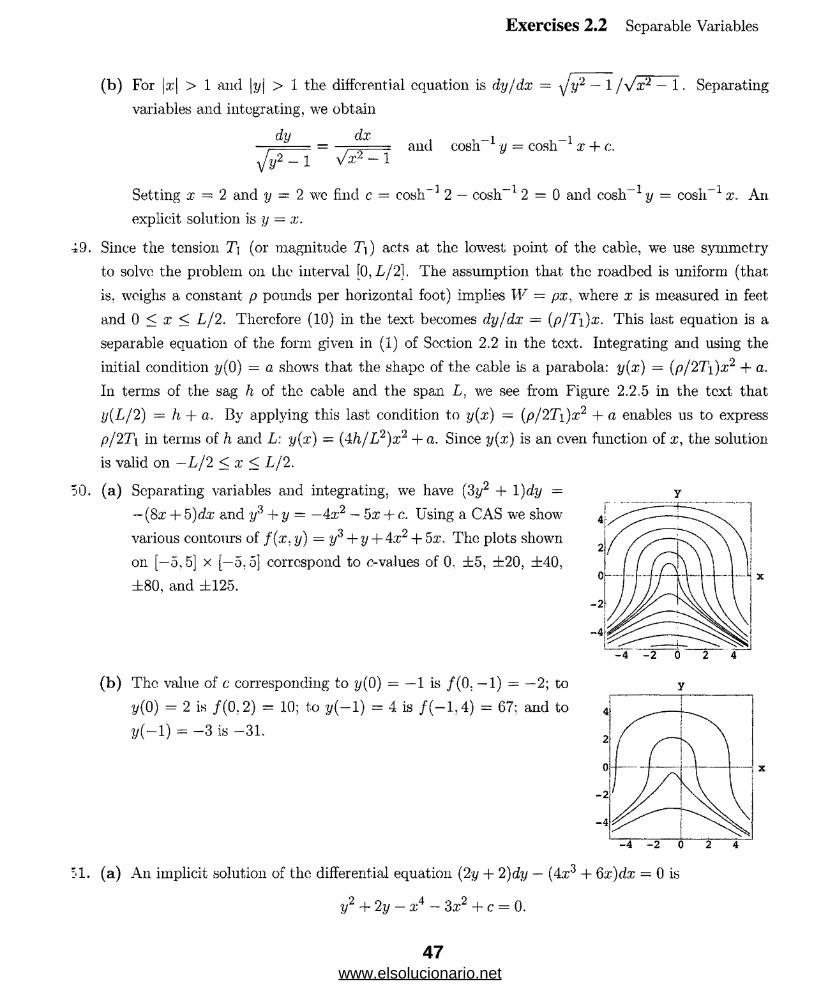
50. (a) Separating variables and integrating, we have (3y2 + 1 )dy =
— (8a; + 5) cite and y3 + y — —4a.-2 — 5x + c. Using a CAS we show
various contours of f(x, y) = y3 + y+ 4a;2 + 5a'. The plots shown
on [—5,5] x [—5.5] correspond to c-values of 0, ±5, d=20, ±40,
±80, and ±125.
(b) The value of c corresponding to y(0) = —1 is /(0. — 1) = —2; to
y(0) = 2 is /(0.2) = 10; to y(—1) = 4 is / (—1,4) = 67: and to
y(—1) = —3 is —31.
51. (a) An implicit solution of the differential equation (2y + 2)dy — (4a:3 + 6x)dx = 0 is
y2 + 2y — a:4 — 3a:2 + c = 0.
y
47www.elsolucionario.net

Exercises 2.2 Separable Variables
The condition y(0) = —3 implies that c = —3. Therefore y2 + 2y — x4 — 3x2 —3 = 0.
(b) Using the quadratic formula we can solve for y in terms of x:
—2 ± a/4-1-4(x4 + 3x2 + 3)
y = ------------~-----------2-------------------------'
The explicit solution that satisfies the initial condition is then
y — — 1 — \Jx4 + 3x3 + 4 .
(c) Prom the graph of f(x) — x4 + 3x3 + 4 below we see that f(x) < 0 on the approximate inter'.--
—2.8 < x < —1.3. Thus the approximate domain of the function
y — —1 — \fx' + Zx + 4 = — 1 — \J f(x)
is x < —2.8 or x > —1.3. The graph of this function is shown below.
£ (x)
(d) Using the root finding capabilities of a CAS, the zeros of / are found to be
—2.82202 and —1.3409. The domain of definition of the solution y(x) is then
x > —1.3409. The equality has been removed since the derivative dy/dx does
not exist at the points where f(x) = 0, The graph of the solution y — <p(x) is
given on the right.
52. (a) Separating variables and integrating, we have
(—2 y + y2)dy = (x — x2)dx
-1 -V f (x;
and9 1 1 1 ^
- V + 3 V = 2 X - r + C -
Using a CAS we show some contours of f(x, y) = 2yi—
6y2 + 2x3 — 3x2. The plots show on [—7,7] x [—5, o]
correspond to c-values of —450, —300, —200, —120,
-60, -20, -10, -8.1, -5, -0.8, 20, 60, and 120.
48www.elsolucionario.net
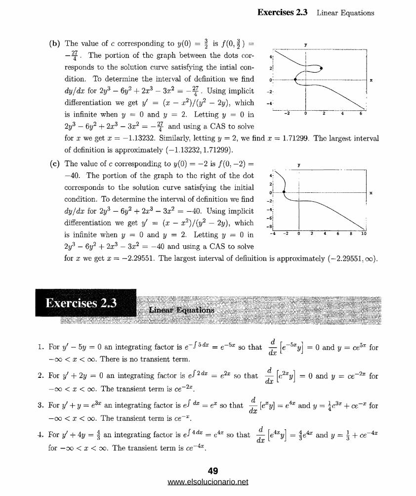
Exercises 2.3 Linear Equations
(b) The value of c corresponding to y(0) = 3 is /(0, | ) =
— . The portion of the graph between the dots cor
responds to the solution curve satisfying the intial con
dition. To determine the interval of definition we find
dy/dx for 2y3 — 6y2 + 2a:3 — 3:r2 — . Using implicit
differentiation we get yf = (x — x2)/(y2 — 2y), which
is infinite when y — 0 and y = 2. Letting y = 0 in
2y:i — 6y2 + 2x'i — 3x2 = — and using a CAS to solve
for x we get x - —1.13232. Similarly, letting y = 2, we find x - 1.71299. The largest interval
of definition is approximately (—1.13232,1.71299).
(c) The value of c corresponding to y(0) = —2 is /(0, —2) = y
—40. The portion of the graph to the right of the dot
corresponds to the solution curve satisfying the initial
condition. To determine the interval of definition we find
dy/dx for 21/3 — 6y2 + 2xi — 3a:2 = —40. Using implicit
differentiation we get y' = (x — x2)/(y2 — 2y), which
is infinite when y = 0 and y = 2. Letting y — 0 in
2y?) — 6y2 + 2a:3 — 3a:2 = —40 and using a CAS to solve
for a: we get x — —2.29551. The largest interval of definition is approximately (—2.29551, oo).
Exercises 2.3
1. For y — by — 0 an integrating factor is e J ocix = e ox so that — [e oxydx L J
—oo < x < oo. There is no transient term.
2. For y1 + 2y — 0 an integrating factor is eJ 2 dx = e2x so that
—oo < x < oo. The transient term is ce 2x.
Adx
<-2xy
= 0 and y = ceox for
= 0 and y — ce~2x for
d3. For y' + y — eix an integrating factor is eJ dx = ex so that — [e'Ty] -- and y - ie3* + ce~x for
dx * 4—oo < x < oo. The transient term is ce x.
4. For y' -f- Ay = 4 an integrating factor is eJ 4 dx == e4x so that [e4xdx L
for — oo < x < oo. The transient term is ce~4x.
V = |e4x and y = A + ce -4x
49www.elsolucionario.net
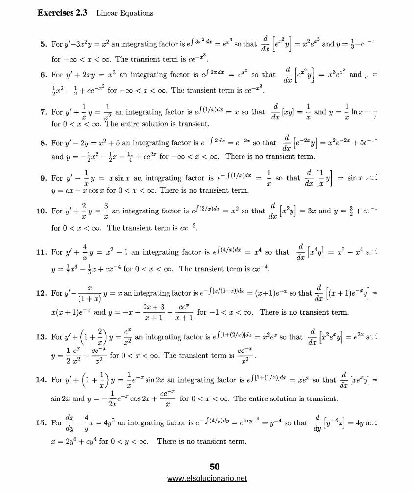
Exercises 2.3 Linear Equations
5. For y'+3x2y = x2 an integrating factor is eJ ,ix dx — e*3 so thatdx
-3e y = x2ef3 and y = |+o.
for — oo < x < oc. The transient term is ce—X
6. For y' + 2xy = x:i an integrating factor is eJ 2xdx — ex so that -r~dx
t 9 O\x? — ^ + CC~X~ for — oo < x < oc. The transient term is ce~x~.
j *e y = £3e* and .. =
1 1 d 1 17. For y' + — y = —~ an integrating factor is — x so that — [xy] = — and y = — In x
x xL dx x xfor 0 < x < oo. The entire solution is transient.
8 . For y' — 2y = x2 + o an integrating factor is e / 2 dx = e 2x so that y - fe 2xy(JLJL
and y = —^x2 - - j + ce2x for — oo < x < oc. There is no transient term.
= x V 2* + O f'
1 1 d 9. For i f ---y = x sin x an integrating factor is e~JO/;r)rf3: = — so that —
•// CLXXy — cx — x cos x for 0 < x < oo. There is no transient term.
2 3
x ' x
for 0 < x < oo. The transient term is cx~2.
1 1 - yx .
= sin a:
10. For i/ + —y = — an integrating factor is eJ (2/a:)rfx = x2 so that x2y| - dx and y = § + c:: t * t ri'r L * J zdx
4 dt11. For y' + — y = :r2 — 1 an integrating factor is eJ (4i*)<lx = x 4 so that — xAy
x ' dx 1 ■
y — — ix + cx-4 for 0 < x < oo. The transient term is cx~4.
= x6 — x4 &:
12. For y'-x d
y = x an integrating factor is e~Nx,/(1+x dx = (x+l)e-a; so that — (x + 1 )e~xy (1 + x) dx l
{X | 3x(x + l)e~x and y = —x — —— — H---— for —1 < x < oo. There is no transient term.
v ' J x + 1 x + 1
( 2 \ €>x ■ d H — ) y = —? an integrating factor is e-l t1+(2/*)]^ _ X2ex so \x2exy
x j xz dx L ' J
2xe a:
1 ex c.e~x
2 x2+ t-2 for 0 < x < oo. The transient term is
ce
x2
14. For y' + (\ + ~') ?/ = —e x sin 2.x an integrating factor is = xex so that [xexy_x x
1 cesin 2x and y — — r—e x cos 2x +
2x xfor 0 < x < oo. The entire solution is transient.
15. For ~ — -x = 4yD an integrating factor is e J(4 dy — elny 4 = y 4 so that -7- \y 4x = Ay a:.:rht fn " ' dy l Jdy y
x = 2y 6 + cy4 for 0 < y < 00. There is no transient term.
50www.elsolucionario.net
Exercises 2.3 Linear Equations
^ + -x = ev an integrating factor is eJ '2 dy — y2 so that -7“ dy y ' dy
2 2 . c cr = -- H— s-e2' + for 0 < y < 00. The transient term is .
y y2 ir ' yz
r dFor y+(tan.x)?y = sec a; an integrating factor is eJ tan x (lx = sec a* so that — [(sec.*) y\ = sec2 x and
dxj = sin x + c cos x for —tt/2 < x < tt/2. There is no transient term.
For 2/ + (cot x)y - sec2 x csc x an integrating factor is eJ cot x dx = eln-smxl = sin a; so thatd - o
[(sin x) y) — sec x and y = sec a; + ccsc x for 0 < x < tt/2. There is no transient term.
T -1- 9 0'T .P~X r fl.For yf + -— ~ y = -—-— an integrating factor is eJ [(x+2)/(x+ )]dx — (x + l)ex. so — \(x + l)exy] =
x + 1 ' x + 1 dxx2 c
2.r and u = ---- e x ---- - e x for — 1 < x < 00. The entire solution is transient.x + 1 x + 1
For y'-\--y - ^ an integrating factor is eJiA/(x+2)\dx — (x + 2)4 so that ~ [(a; + 2)4yl =x + 2 (x + 2)2 0 v J dx Lv 1
~v.x + 2)2 and y - ^(a; + 2)_1 + c(x + 2)~4 for —2 < x < o o . The entire solution is transient, o
dvFor — + r see 6 — cos 9 an integrating factor is eJ s<]c()d0 = ein |seen-tan_ sec q _|_ tan/9 so that
dt)
~ [(sec 9 + tan 6)r] — 1 + sin 9 and (sec 9 + tan 9)r = 9 — cos 9 + c for —tt/2 < 9 < 7t/2 . i d
For + (21 — 1 )P — 4t — 2 an integrating factor is g/(2t-1)rff = so that dt dt
■it — 2)et and P = 2 + cei_ r for —oc < t < 00. The transient term is ce*-t .
For 1/+ ( 3 + — y = --- an integrating factor is e-/ [•i+(1/T)i,il: = xc*x so that — [xe3:ryj - 1 andV xJ x dx L ' J
o , >.7 = e H----- for 0 < x < oo. The entire solution is transient.
x
For 1/ + ^ y = £ J lJ : an integrating factor is e/i2/ ^ '-1)]*' = -— 1 so that — x* - 1 x - 1 x + 1 dx
and (:/: — 1 )y = x(x + 1) + c(x -f 1) for — 1 < x < 1.
For y' + - y = — ex an integrating factor is e f^ ^ :)dx — x so that ~ \xy\ - ex and y = —ex + — x x dx ' ’ x x
1 2 — e:or 0 < x < oc. If y(l) = 2 then c = 2 — e and y = —ex H---- -.
x x
For ~ x = 2y an integrating factor is e~ }(l/y)dy _ i so that — dy y y dy
° f - l P
x — 1X + 1 .
= 1
—Xy
- 2 and x = 2y2 + ay49
for 0 < y < 00. If y( 1) = 5 then c = —49/5 and x ■ 2y2 — — y.5
For f-j- + y I = T~ an integrating factor is eJ dt = eRt/L So that — \eRt' L i] — —eRt/L and dt L L dt 1 1 L
51www.elsolucionario.net

Exercises 2.3 Linear Equations
E
R
dT
i = ^ - + ce Rt/L for —oc < t < oc. If v'(0) = tQ then c = i o — E/R and i = — + ( i $ — — 'j R R. \ R J
E
R
d r - i28. For —-- kT = —Tmk an integrating factor is k dt = e kt so that 4- fe kiT] - —Trnke kt an:(it dt
T - Tm. + cekt for —oo < t < oo. If T(0) - To then c = 7q — Tm and T = Tm + (To — Tm)ekt.
29. For ?/ H-- —rV = —— r an integrating factor is = x + 1 so that ~-\(x + l)y| =x +1 x +1 dx
X X clnx and y = ——— In a,’ --- —- H---— for 0 < x < oc. If y(l) = 10 then c = 21 and
&- + 1 x + 1 x + 1
21X _ xy = ---- hi x -x + 1 x + 1 ' x + 1
30. For i/+(tana)y = cos2 x an integrating factor is e-ltanx<ir = ein|secx| — sec x so that — [(seex) y] =f.AtJU
cosx and y = sin x cos x + a cos x for —tt/2 < x < tt/2. If y( 0) = —1 then c = —1 and y =
sin x cos x — cosx.
31. For y' + 2y = f(x) an integrating factor is e2x so that
e2x = { ie2x + ci, 0 < x < 3
W x > 3.
If y(0) - 0 then c\ = —3/2 and for continuity we must have
C2 — |e6 — | so that
| i ( l -e~2x), 0 < x < 3
V [ |(e6 - l)e~2a\ x > 3.
32. For y' -f y = f(x) mi integrating factor is ex so that
ex + ci, 0 < x < 1
—ex + C2, x > 1.
If y(0) = 1 then cj. = 0 and for continuity wc must have C2 = 2e
so that
1 * - -
y e x =
1. 0 < x < 1y =
2e1~x - 1, x > 1.
33. For y' + 2xy = /(x) an integrating factor is ex so that
2 f \ex~ + c\, 0 < x < 1 ye: =
{ 02, X > 1.
If y(0) = 2 then cj = 3/2 and for continuity we must have
C'2 = + 5 so that
52www.elsolucionario.net

Exercises 2.3 Linear Equations
4 . For
, 2x
y + T T * y
v
X
i + fe - L,
(he +1) 0 < x < 1
x > 1.
1 + X2 '—x
1 + X2 ''ii integrating factor is 1 + x2 so that
0 < x < 1
x > 1,
-1 —
( l + x2) y =0 < x < 1\x? + ci,
~ lx 2 + C2, X > 1.y(0) = 0 then ci = 0 and for continuity wc must have C2 = 1 so that
r i i
y -2 2(1 + x2) ’
0 < x < 1
[ 2 (1 + x2) 2
1: . *.Ve first solve the initial-value problem y' + 2y = 4a:. y(0) = 3 on the interval
j. 1]. The integrating factor is cJ 2dx = e2x. so
4-[e2xy} = ixe2x dx
i2xy - j 4xe2xdx - 2xe2x — e2x + C\
- 2 xy = 2x — 1 + c\e
Vsing the initial condition, we find y(0) = — 1 + c\ = 3, so c\ = 4 and
, = 2x — 1 + 4e-2x, 0 < x < 1. Now, since y(l) = 2 — 1 + 4e~2 = 1 + 4e~2,
-re solve the initial-value problem y' — (2fx)y = 4a;, y( 1) = 1 + 4e-2 on the
interval (1. oo). The integrating factor is eJ(-‘2/x)eix - c-2in* _ x-2 s0
d . i _o 4 - [* t i = 4 x X - = -
-2 f 4* y = I ~ dx = 4 In a: +
7 a:
y = Ax2 In x + C'yx2.
C2
We use In a; instead of In |a;| because x >1.) Using the initial condition wc find y(l) = — l+4<? 2,
' ij = 4:r;2 In a: + (1 + 4e_2).x2, x > 1. Thus, the solution of the original initial-value problem is
53www.elsolucionario.net
Exercises 2.3 Linear Equations
( 2x — 1+ 4e~2x. 0 < x < 1
^ \ 4.r2 In x + (1 + 4e_2)a;2. x > 1.
See Problem 42 in this section.x ___36. For y' + exy = 1 an integrating factor is ee . Thus
d r - ,.X , . X f X t— [( ' y\ = e and e y = / e dt + c. dx ' Jo
From 2/(0) = 1 we get a = e, so y = e-6* Jq ee dt + e1- .
When y' + exy = 0 we can separate variables and integrate:
— = —ex dx and In lyj = — ex + c.V
Thus y = c\e~ . Prom y(0) = 1 we get ci = e, so y = e1-e .
When if + exy = ex we can see b,y inspection that y = 1 is a solution.
37. An integrating factor for y' — 2xy = 1 is e~x . Thus
2 rx ,2 \Fir e~x y = / e d i = ~- erf(z) + c
*/ 0 a
y = ~~ex crf(x) + cex .&
From y(l) = (v/7r/2)e erf(l) + ce = 1 we get c = e-1 — ^ crf(l). The solution of the initial-va/:
problem is
y = ^e^erffa) + (e~l - ^ e r f ^ e * 2
= ex -1 -r ex~(erf(x) — erf(l)). z
38. We want 4 to be a critical point, so we use y' = 4 — y.
39. (a) All solutions of the form y = x°ex — x4ex 4- cx4 satisfy the initial condition. In this caf-
since 4/x is discontinuous at x = 0, the hypotheses of Theorem 1.2.1 are not satisfied and t:
initial-value problem does not have a unique solution.
(b) The differential equation has no solution satisfying y(0) = (jq . yo > 0.
(c) In this case, since .-eo > 0, Theorem 1.2.1 applies and the initial-value problem has a unic
solution given by y = x^ex — x4ex + c.r4 where c : vq/xq — XQex° + ex°.
40. On the interval (—3,3) the integrating factor is
ej x d x / ( x 2—9) _ e - f x d x / ( 9 - x 2) _ g £ ln ( 9 - x 2) _ ^ /g _ ^.2
54www.elsolucionario.net

Exercises 2.3 Linear Equations
and sod
dxv'o" x2y - 0 and y =
V9 —a:.2
We want the general solution to be y = 3x — 5 4- ce x. (Rather than e x, any function that
approaches 0 as x —>• oo could be used.) Differentiating we get
y' = 3 — ce-* = 3 — (y — 3a: + 5) = —y -f- 3x — 2,
so the differential equation y1 + y = 3x — 2 has solutions asymptotic to the line y = 3.x — 5.
The left-hand derivative of the function at x = 1 is 1/e and the right-hand derivative at x = 1 is
1 — 1/e. Thus, y is not differentiable at x = 1.
(a) Differentiating yc = c/a:3 we get
3cy'c X41so a differential equation with general solution yc = e/.r3 is xy' + 3y = 0. Now
xy'p -f 3yp = x(3x2) + 3(.x3) = 6a:3
so a differential equation with general solution y — c/x3 + z3 is xy' -j- 3y = 6a:3. This will be a
general solution on (0, oo).
(b) Since y( 1) = l 3 — l / l 3 = 0, an initial condition is y( 1) = 0. Since
1/(1) = l 3 + 2/13 = 3, an initial condition is y(l) = 3. In each
case the interval of definition is (0, oc). The initial-value problem
xy' + 3y = 6a:3, y(0) = 0 has solution y = a:3 for —oo < x < oo.
In the figure the lower curve is the graph of y(x) — a;3 — 1 /a:3.while
the upper curve is the graph of y = x3 — 2/a:3.
(c) The first two initial-value problems in part (b) are not unique. For example, setting
1/(2) = 23 - 1/23 = 63/8, we see that y(2) = 63/8 is also an initial condition leading to
the solution y = a:3 — 1/a:3.
Sincc ef p(x)dx+c = ec€f P(z)dx _ CieJ P{x)dX' we wou](j have
cie-f p(x)dxy = C2 + J ^ ^ m d x and e^p^ dxy — cz + J eJ p^ cla: f(x) dx,
which is the same as (6) in the text.
We see by inspection that y = 0 is a solution.
The solution of the first equation is x = eie_Al*. From a;(0) = x q we obtain ci = x q and so
x — X Q e~ X l t . The second equation then becomes
dy4r = c — A-2y dt
55www.elsolucionario.net
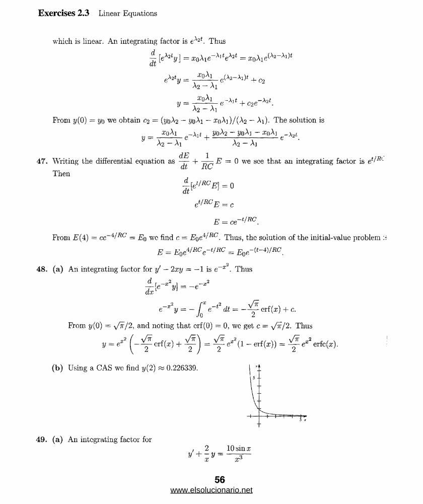
Exercises 2.3 Linear Equations
which is linear. An integrating factor is e*2*. Thus
y [ex'2ty] = xoAie = aroAie^2 ^Cot*
M y = ^ Ai e(A2-Ai)f + ^
A2 - Ai
.x'oAi. e“Ajt_|_c g A'2<_
A2 -Al
From y(0) = yo we obtain C2 = (yoAa — yoAi — £oA])/(A2 — Ai). The solution is
_ sqAi e_Alt + ypA2 - ypA] - rcpA] ^_Aa/,
A2 — Ai A2 — Aj
d.E 147. Writing the differential equation as —— h jE7 = Q we see that an integrating factor is et/Rl
do J- i-OThen
A[el:/RCE} = 0 dt
ef!RCE = c
E = ce~t/RC.
From E(4) = ce~4/ Rc = Eq w c find c: = Eoe^Rc. Thus, the solution of the initial-value problem
E = E0e^RCe ^ RC = E^ - ^ RC.
48. (a) An integrating factor for y' — 2xy = —1 is e~x2. Thus
d r _ r 2 2" v\ = ~e
ypKe x y = — J e 1 dt = — erf (z) + c.
From y(0) = v/tt/2, and noting that crf(0) = 0, we get c = a/ tt/ 2. Thus
V = e’ ! orfM + I f ) = T f - el{(x» = X e' 2 erfo(a:)'
(b) Using a CAS wc find y(2) 0.226339.
49. (a) An integrating factor for, 2 10sin:r
y + - y =a; .T
56www.elsolucionario.net
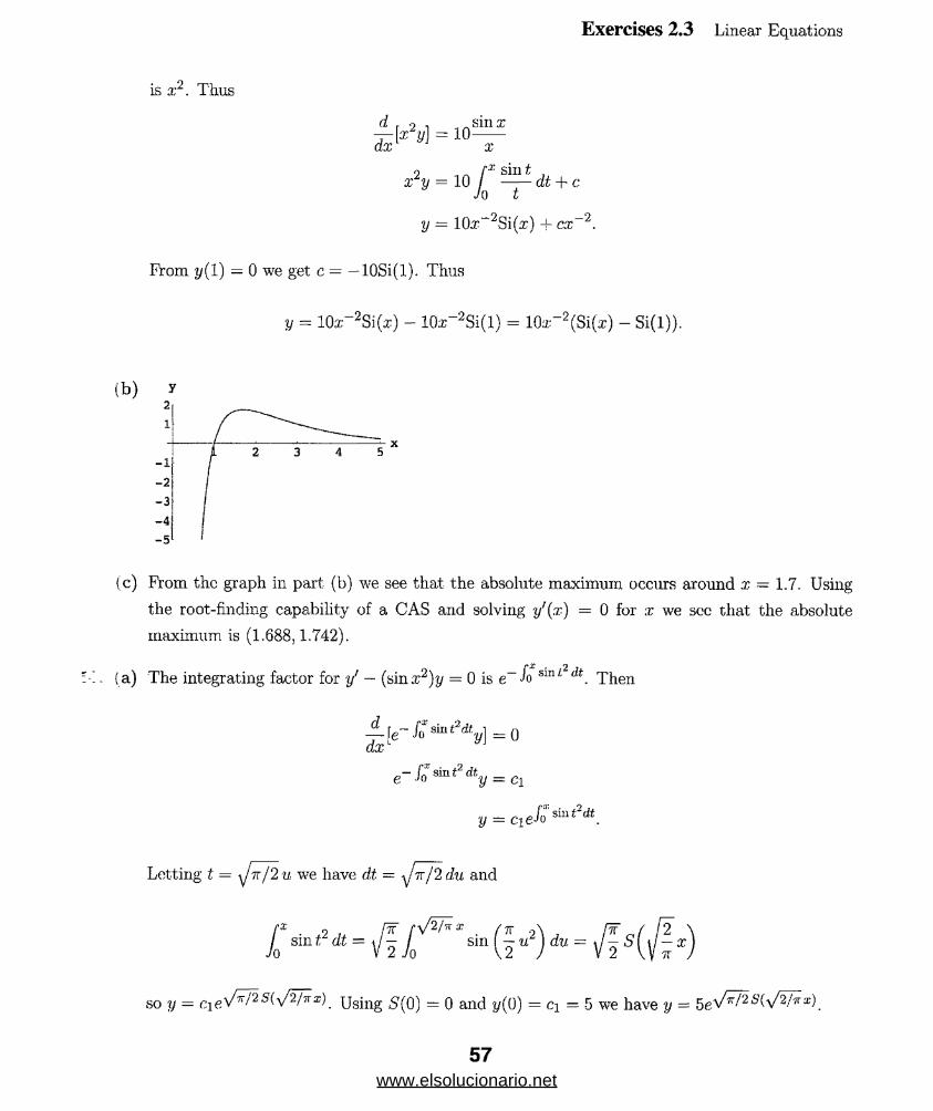
Exercises 2.3 Linear Equations
is x2. Thus
o „. rx sin t , x y = 10 ---dt + c
J Jo t
y = 10# 2Si(;r) + ex 2.
Prom y(l) = 0 we get c = — 10Si(l). Thus
y = 10.x“2Si(#) - 10x_2Si(l) = 10a.r2(Si(ir) - Si(l)).
( b ) y
r x >-1-2
-3-4“5
(c) From the graph in part (b) we see that the absolute maximum occurs around x — 1.7. Using
the root-finding capability of a CAS and solving yf(x) = 0 for x we sec that the absolute
maximum is (1.688,1.742).
so y = 7*x)m Using 5(0) — 0 and y(0) = c\ — 5 we have y =
2
1
r X . 9
( a) The integrating factor for y' — (sinx2)y = 0 is e~Jo . Then
y = CleJosint2dt
57www.elsolucionario.net
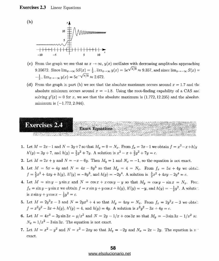
Exercises 2.3 Linear Equations
(c) From the graph wc see that as x —► oc, y(x) oscillates with decreasing amplitudes approaching
9.35672. Since limx- oo 5S(x) = \ , linij;-*^ y(x) — 9.357, and since lima;_i._oc S(x) =
— , lim ^-^c y(x) = 5e-v/ /8 & 2.672.
(d) From the graph in part (b) we see that the absolute maximum occurs around x = 1.7 and tlic-
absolute minimum occurs around x = —1.8. Using the root-finding capability of a CAS anc
solving y'(x) = 0 for we see that the absolute maximum is (1.772,12.235) and the absolute
minimum is (—1.772,2.044).
1. Let M = 2x — 1 and N = 3y+7 so that My = 0 = Nx. From fx = 2x— 1 we obtain / ~ x2—x+h(y
h\y) = 3y -j- 7. and h(y) = §y2 + 7y. A solution is x2 — x + ^y2 + 7y = c.
2. Let M = 2x + y and N — —x — 6y. Then My = 1 and Nx = —1, so the equation is not exact.
3. Let M = 5.7; + 4y and N — 4x — 8y3 so that My — 4 = N:r. From fx = ox + 4y wc obtai:
/ ■ |:/:2 + 4xy + h(y), h'(y) — —8y3, and /i(y) = —2y4. A solution is |:t'2 + 4a;y — 2y4 = c.
4. Let M = siny — ysinx and JV = cosx + a; cosy — y so that My ~ cos y — sin a; = Nx. Fro:;
fx = siny — y sin x we obtain / = xsiny+ ycosx-^h^y). h\y) — —y, and h(y) = —\y2- A solutic
is x sin y -j- y cos x — \y2 = c.
5. Let M = 2y2x — 3 and N = 2yx~ + 4 so that M tJ = 4xy = Nx. From fx = 2y2x — 3 we obta::
/ = x2y2 — 3x + h.(y), h'(y) = 4. and h(y) — Ay. A solution is x2y2 — 3x 4- 4y = c.
6. Let M = Axd — 3y sin 3x — y/x2 and N = 2y — 1/x + cos 3x so that My = —3 sin 3a; — 1 jx2 ai.
Nx — 1 jx2 — 3 sin 3a;. The equation is not exact.
7. Let M = x2 — y2 and N = x2 — 2xy so that My = —2y and Nx — 2x — 2y. The equation is n "
exact.
58www.elsolucionario.net

Exercises 2.4 Exact Equations
Lot M — 1 + In x + y/x and N = — 1 -f In x so that My — 1/x = Nx. From fy = — 1 + In x we obtain
= —y + y Inx + h(y), h'(x) = 1 + lna:, and h(y) = a:lux. A sohition is —y + y Inx + x Inx = c.
Let M = y3 — if sin x — x and N = 3xy2 + 2y cos x so that My = 3y2 — 2y sin x = Nx. From
= y3 — y2 sin x — x we obtain / = a:y3 + y2 cos x — \x2 + h(y). h'(y) = 0, and h(y) = 0. A solution
xy3 + y2 cos x — ^x2 = c.
Let M = xs + y3 and N = 3xy2 so that My = 3y2 = Nx. From fx = x3 + y3 we obtain
■’ = jf.r4 + xy3 + h(y), h'(y) = 0, and h(y) = 0. A solution is |a:'* + xy3 = c.
Let M = ylny — e~xy and N = 1/y + xlny so that My = 1 + lny + xe~xy and Nx = lny. The
equation is not exact.
Let M = 3x2y + el! and N = x3 + xey — 2y so that My = Zx* + ev = Nx. From fx = 3x2y + ey we
:btain / = x3y -j- xev -f- h(y), h'{y) = —2y. and h(y) = —y2. A solution is x3y + xey — y2 = <:.
Let M = y — 6x2 — 2xex and N = x so that My = 1 — Nx. From f x = y — 6a-2 — 2xex we obtain
= xy — 2x3 — 2xex + 2ex + h(-y), h!{y) = 0. and h(y) ~ 0. A solution is xy — 2x3 — 2xex + 2ex = c.
Let M = 1 — 3jx + y and N = 1 — 3jy + x so that My = 1 = Nx. From fx = 1 — 3/x + y3
-.vc obtain f = x — 3In |:r| + xy + h(y), h!(y) = 1 — and h(y) = y — 3In |;y|. A solution is
-r y + xy-3 In \xy\ = c.
Let M = x2y3 — 1 /( l + and N = x3y2 so that My ■ 3xzy2 = Nx. From
V = x2y3 — 1/ ( 1 + 9:c2) wo obtain / = ^x^y3 — ^ arctan(3a:) + h(y), h.'(y) = 0, and h(y) = 0.
A solution is x3y3 — arctan(3a:;) = c.
Let M = —2y and N = by — 2x so that My = — 2 = Nx. From fx = —2y wc obtain / = —2xy+h(y).
V(y) = 5y, and h(y) = |y2. A solution is —2xy + %y2 = c.
Let M = tana; — siuicsiny Mid N = cosx cosy so that My = — sin.rcosy = Nx. Rrom
tx -- tanx — sin a: siny wc obtain / = In | sec a* | + cos x sin y + h(y), h'(y) = 0, and h(y) = 0. A
solution is In | seca;| + cos a: siny = c.
Let M = 2y sin x cos x — y + 2y2exy~ and N = — x + sin2 x + 4xyexy~ so that
My = 2 sin a: cos .x — 1 + 4xy3exy2 + 4yexy2 — Nx.
t o 2From fx = 2ysinaj cos a; — y + 2y2exy~ we obtain / = y sin x — xy + 2exy + h(y), h'(y) = 0. and
h(y) = 0. A solution is y sin2 x — xy + 2exy2 — c.
Let M — 4t3y —15 2 — y and N = t4 + 3y2 — t so that M tJ = At3 — 1= Nt. From f t = At3y — 1512 — y
wc obtain / = t4y-bt3 —ty + h(y), h?(y) = 3y2, and h(y) — y?>. A solution is tS j-ot3-ty+y3 = c.
Let M = 1/t + l/ t2 — y/ (l2 + y2j and N = ye!/+tf (t2 + y2j so that My = (y2 — t2j j (t2 + y2 =
-Yf. From f) = 1/t + I ft2 — yj (t2 + y2 we obtain / = In\t\ — ^ - arctan + h(y), h'(y) = yey,
59www.elsolucionario.net
Exercises 2.4 Exact Equations
and h(y) — yey — ey. A solution is
In \t\ — ^ — arctan + yey — ey = c.
21. Let M = x2+2xy+y2 and N = 2xy+x2 — 1 so that My = 2(x+y) = Nx. From fx = x2+2xy+y2 w-.1
obtain / = ^£3+x2y+xy2+/?. (y), h\y) — —1, and h(y) — —y. The solution is ^xli+x2y+xy2—y - c
If 2/(1) = 1 then c = 4/3 and a solution of the initial-value problem is + x2y + xy2 — y = | .
22. Let M — ex + y and N = 2 + x + ye?; so that- My = 1 = Nx. From fx = ex + y we obtair.
f = ex + xy + h(y). h'(y) = 2 + ye1', and /i(y) = 2y + yey — y. The solution i-
ex + xy + 2y + yev — ev = c. If y(0) = 1 then c = 3 and a solution of the initial-value prob
lem is ex + xy + 2y + yey — ey = 3.
23. Let M = Ay + 2t — 5 and N = 6y + At — 1 so that My = A = Nt- From ft = Ay + 2t — 5 we obtai:.
f = Aty+t2— ht+h(y). h'(y) — 6y — 1, and h(y) = 3y2 — y. The solution is Aty+t2 — 5t+3y2 — y = <
If y(—1) = 2 then c = 8 and a solution of the initial-value problem is Aty + t2 — bt + 3y2 — y = 8.
24. Let M = £/2y4 and N = (3y2 — i2) /y° so that My = —2t/y5 = Nt. From ft = t/2y4 wc obtai:.
t2 3 3 t2 3+ % ) , h\y) = p , and h(y) = ■ The solution is 4^4 “ 2 2
_____3 _ _ _ 5
4y4 2y2 A
25. Let M = y2 cos x — 3x2y — 2x and N = 2y sin a;- — £3 + In y so that My = 2y cos x — 3:r;2 = Arx- Fror..
fx = y2 cos a: — 3x2y — 2ar we obtain / = y2 sin x — x^y — x2 + h(y). h!(y) = In y, and h(y) = y In y — t.
The solution is y2 sin x — x^y — x2 + y In y — y = c. If y(0) = e then c = 0 and a solution of tl:-
initial-value problem is y2 sin x — x^y — x2 + y lny — y = 0.
26. Let M = y1 + y sin x and N = 2xy — cos x — 1/ 1 + y2 so that My = 2y + sinrr = Nx. Fron.
fx = y2 + ysin.x we obtain / = xy2 — ycosx + h(y), h'(y) = 9 , and h(y) = — tan-1 y. Tk-
solution is xy2 — ycosx — tan_1y = c. If y(0) = 1 then c = — 1 — 7t/4 and a solution of tli-7r
initial-value problem is xy2 — ycosx — tan-1 y = -1 — - .
27. Equating My = 3y2 -I- 4toy3 and Nx = 3y2 + 40:cy3 we obtain k = 10.
28. Equating My = 18xy2 — siny and Nx = Akxy2 — siny we obtain k — 9/2.
29. Let M = —x2y2 sin x + 2xy2 cosx and N = 2x2y cos x so that My = —2x2ysm x + Axy cos x — A'
From fy = 2x2y cos x we obtain / = x2y2 cos x + h(y), h'(y) = 0, and h(y) = 0. A solution r
the differential equation is x2y2 cos x = c.
30. Let M = (x2 + 2xy — y2) / (x2 + 2xy + y2) and N = [y2 -f- 2xy — x2 / [y2 + 2xy + x2j so thtf
My - —4xy/(x + y)3 = Nx. From fx = (x2 + 2xy + y2 — 2y2) / (x + y)2 we obtain
f = + h (y)-, ti(v) = 7^ and Kv) = -7^2 ■ The solution is o _ 0 2 = c- y(!) = 1 the:
c = —5/4 and a solution of the initial-value problem is 4 2
60www.elsolucionario.net
f = x H------ (- A(y), = —1, and /i(y) = —y. A solution of the differtiiria. -r >x + y
x2 + y2 = c(x + y).
31. We note that (My — A^/AT = 1/a:, so an integrating factor is eJ dx/x = x. Let M = — ; *
and N = 2x2y so that My = Axy — Nx. Prom fx — 2xy2 + 3x2 we obtain / = — .r; — .
h'(y) - 0, and h(y) = 0. A solution of the differential equation is x2y2 + :r3 = c.
32. We note that (My — Nx)/N = 1, so an integrating factor is e fdx = ex. Let M = xyex — y-*~ — .. ?
and N = xex + 2yex so that My — xex + 2yex + ex = Nx. Prom fy — xex + 2yex we ::
/ — xyex + y2ex + h(x), h!(y) - 0, and h(y) = 0. A solution of the differential equa:: .:. >
xyex + y2ex = c..
33. We note that (A^ ■ My)/M = 2/y, so an integrating factor is e f2dy/y — y2. Let M = 6 .nr'
N = 4y3 + 9x2y2 so that My = 18xy2 = Nx. From fx = 6xy3 we obtain / = 3x2y3 — : -
h!(y) - 4y3. and /i(y) = y4. A solution of the differential equation is 3x2yA — y4 = c.
34. We note that (My — Nx)/N = —cota;, so an integrating factor is e- J cotxdx = escx. 1 .'
Af = cos x csc x = cot x and N = (1 + 2/y) sina;csca: = 1 + 2/y. so that My = 0 = A*r. F: ::;.
fx — cot a.- we obtain / = hi (sin x) + h(y). h?(y) = 1 + 2/y, and /?<(y) = y + lny2. A solution of t..-
differential equation is In (sin a:) + y + lny2 = a.
35. We note that (My — Nx)/N = 3, so an integrating factor is eJ3(lx — e3x. Let
M = (10 — 6y + e-3a:)e3: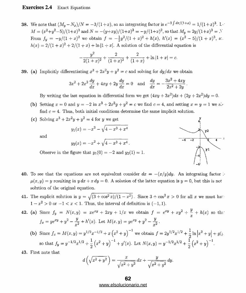
Exercises 2.4 Exact Equations
38. We note that (My — Nx)/N = —3/(1 +&), so an integrating factor is e_3/ <i'r/(1+x') = 1 j (1+$)^. L-'
M = (x2+y2-l5)/(l+x)3 and N = -(y-rxy)/(1+x)3 — —y/(l+x)2, so that My = 2y/(l+x)3 - V
From fy = —y/( 1 + x)2 wc obtain / — —\y2/{\ + x)2 + h(x). h'(x) = (x2 — 5)/(l + x)3, a:.
h(x) = 2/(1 + x)2 + 2/(1 + x) + In 11 — x\. A solution of the differential equation is
yrro + ro + + In |1 + d = c.
2(1 + x)2 (1+x)2 (l + z)
39. (a) Implicitly differentiating x3 + 2x2y + y2 = c: and solving for dy/dx we obtain
. 9 ~ dy , „ dy , dy 3x2 + Axy
3x~+ 2x fa + 4x1 + 2y d i = 0 “ d S =
By writing the last equation in differential form we get (4xy + 3x2)dx + (2y + 2x2)dy = 0.
(b) Setting x = 0 and y = —2 in ;c3 + 2x2y + y2 = c we find c = 4, and setting x = y = 1 we air-
find c = 4. Thus, both initial conditions determine the same implicit solution.
(c) Solving x3 + 2x2y + y2 = 4 for y we get
yi(x) = —a;2 - yj4 — x3 + x4
and
•y2( ‘) = -x2 + \/A —x3 + x4 .
Observe in the figure that y-\ (0) = — 2 and y2(l) = 1-
40. To see that the equations are not equivalent consider dx = —{x/y)dy. An integrating factor
/.i(x. y) = y resulting in ydx + xdy = 0. A solution of the latter equation is y = 0, but this is not
solution of the original equation.
41. The explicit solution is y ~ y (3 + cos2a:)/(l — .x-2) . Since 3 — cos2 x > 0 for all x we must hav
1 — x2 > 0 or —1 < x < 1. Thus, the interval of definition is (—1,1).
42. (a) Sincc f y = N(x,y) - xexy + 2xy + 1/x we obtain / = exy + xy2 -f- — + h(x) so the.-X
,.2 y i ut/~\ t a ........ xy i „,2___y_,2fx = yexy + y - ^2 + h'(x). Let M(x, y) = ycxy + - 3 •
- 1
(b) Since f £ — M(x, y) = yi>l2x 1,11 + x (x2 + yj we obtain / = 2yl^2x1-'2 + ^ In |.x2 + y\ -+- g{i£
so that fy = y~1/2xl/2 + ^ (.r2 + y) 1 + g'{x). Let N(x, y) = y~1’2x1/"2 + ^ (x 2 + yj
43. First note that/ f—--- - \ x
: dx +d [ Jx 2 + y2 =y
yxz -I- yz■ dy.
62www.elsolucionario.net
Exercises 2.4 Exact Equations
Then x dx + y dy = \Jx2 + y2 dx becomes
, dx A— r~y — dy = d ( J x 2 +y2\ — dx.j x 2 + y2 j x 2 + y2 ' Vv J
The left side is the total differential of \jx2 + y2 and the right side is the total differential of x + c.
Thus \Jx2 + y2 = x + c is a solution of the differential equation.
To see that the statement is true, write the separable equation as —g(x) dx+dy/h(y) = 0. Identifying
M = —g(x) and N = l/h(y), we see that My = 0 = Nx. so the differential equation is exact.
(a) In differential form we have (v2 — 32x)dx + xv dv = 0. This is not an exact form, but fi(x) — x
is an integrating factor. Multiplying by x we get (xv2 — 32x2)dx -j- x2v dv = 0. This form is
the total differential of u = \x2v2 — 4j=.r3. so an implicit solution is \x2v2 — = c. Letting
x = 3 and v = 0 we find c = —288. Solving for v we get
V3v = 8
(b) The chain leaves the platform when x — 8, so the velocity at this time is
. 3 64
(a) Letting
M(x,y) = 02xy, 9 and N(x,y) = 1 + V X(x2 + y2)2 ' ’ ‘ (x2 + y2)2
we compute
_ 2x3 - 8xy2 _(xz -+- yA)6
so the differential equation is exact. Then we have
% = M<*. V) = p f w = 2xp(x2 + s,2)“ 2
/ O ,y) = -v(x2 + v2) 1 + 9(y) = - 2T 9i2 + sfo)
d f y2 - x2 , y2 - x2+ 9 (y) = ^ («, y) = i + T
dy (x2 + y2)2 ' * (x2 + y2)2 '
VThus, g'(y) = 1 and g(y) = y. The solution is y — x2 _^, o = c■ When c = 0 the solution is
x2 + y2 = 1-(b) The first graph below is obtained in Mathematica using f(x, y) —y — y/(x2 + y2) and
ContourPlot[f[x, y], {x, -3, 3}, {y, -3, 3},
63www.elsolucionario.net
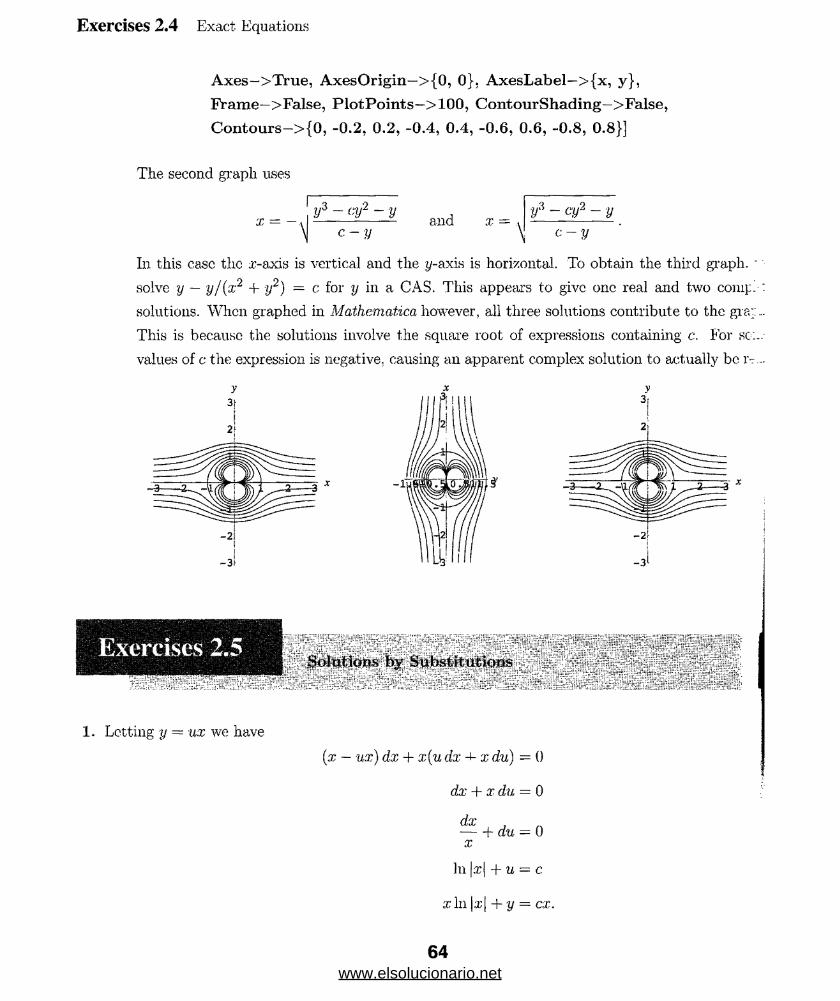
Exercises 2.4 Exact Equations
Axes—>True, AxesOrigin—>{0, 0}. AxesLabel—> (x, y}, Frame—>False, P lotPoints—> 100, ContourShading—>False,
Contours—>{0, -0.2, 0.2, -0.4, 0.4, -0.6, 0.6, -0.8, 0.8}]
The second graph uses
x = —yz - <ni2 - y
c- yand x —\
•y3 - cy2 - y
c - y
In this ease the x-axis is vertical and the y-axis is horizontal. To obtain the third graph. '
solve y — y/(x2 + y2) = c for y in a CAS. This appears to give one real and two coni};.
solutions. When graphed in Mathematica however, all three solutions contribute to the gra::
This is because the solutions involve the square root of expressions containing c. For so:,
values of c the expression is negative, causing an apparent complex solution to actually be i-
\ / ' "7 \ ~ } V;'' f- ‘ v.: ::j~; V- ”~ : r r l " : - ”. Vj;>r ^ y
ScilMiojas by Siibstittttloris'"'J' . '' v *'* ' * .• -V j - . ' ”, »7~ ' * .
\ *; •/.: -V** \ . \... r ; . /V:; ;; ;:/r ,;r
1. Letting y — ux we have
(x — ux) dx + x(u dx x du) - 0
dx + x du = 0
dx---1- du — 0x
111 l-xl + u = c
x In |a;| + y = ex.
64www.elsolucionario.net
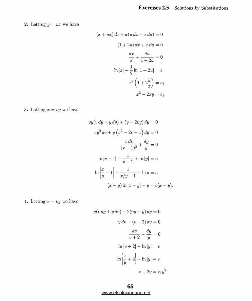
Exercises 2.5 Solutions by Substitutions
2. Letting y = ux we have
(x + ux) dx + x{u dx + x du) = 0
(1 + 2-u) dx + x du = 0
dx du-- h ---—x 1 + 2u
= 0
In |x| + - In |1 + 2u\ = c
rr2 ( l + 2| ) = C
x1 + 2 xy = ci.
3. Letting x = vy we liavc
vy{v dy + y dv) + (y - 2vy) dy = 0
vy2 dv + y (y2 - 2v + l) dy = 0
vdv + rfy = ()
In
In \v — 1|
x
(u - l )2 y
1
y
v - l
1
x/y- 1
+ In \y\ = c
+ lny = c
(x - y) In \x -y\-y = c(x - y).
4. Letting x = vy wc have
y(v dy + ydv) — 2 (vy + y) dy = 0
y dv — (t> + 2) dy = 0
dv _ dy ^ 0
v + 2 y
In \v + 2| — In \y\ = c
Inx
+ 2; - In \y| = c
x + 2y = ciy
65www.elsolucionario.net

Exercises 2.5 Solutions by Substitutions
5. Letting y = ux wc have
(u?x2 + ux2j dx — x2(u dx -r x du) = 0
u2 dx — x du = 0
dx d u _9 uX v>
In |.t | + — = cu
In Irrl + — = cV
y In \x\ + x = cy.
6. Letting y - ux and using partial fractions, we have
( u2x2 + ux2'} dx + x2 (u dx + x du) = 0
x2 (v? + 2 it} dx + x3du = 0
dx du— + “ 7---= 0x u(u + 2)
In |jc| + ^ In | w[ — ^ In \u + 2| = c
ci
X \ x,2„ _
7. Letting y = ux wc have
xry = c\ (y + 2x).
(ux — x) dx — (ux + x) (udx + x du) = 0
(u2 + l) dx + x(u + 1) du = 0
dx u + 1 ,— + -s— - du = 0 x u2 + 1
In jx| + ^ In (u2 + l) + tan-1 u = c
lnx2 + 1 + 2 tan-1 - = c±
In fa;2 + y2) + 2 tan 1 — = c\.' ' x
66www.elsolucionario.net

Exercises 2.5 Solutions by Substitutions
(a; + 3ux) dx — (3a- -+■ ux) (u dx + x du) = 0
('u2 — l) dx + x(u + 3) du = 0
dx it + 3---h 7---—rz--- r r du = 0X (u — l ) ( l l + l )
In |.-r) + 2 In \u — 1| — In |u + 1) = c
x(u — l) 2
Letting y = ux we have
u 4- 1= Cl
(y - x f = c.i{y -+ x).
Letting y = ux we have
—ux dx + (x + \fu X') (u dx + x du) = 0
(x2 + ) du + xu^'2 dx = 0
1\ , dx(V3/2 + i U + * = 0V u) x
—2w-1/2 + In \u\ + In |x| = c
In \y/x\ + In |xj = 2\jxfy + c
y(ln \y\ - c)2 = 4x.
Letting y = ux we have
(uz + \jx2 — (ux)2 ) da: — x(udx + xdu) du = 0
\/x2 — u2x2 dx — x2 du = 0
x\j 1 — u2 dx — x2 du — 0, (x > 0)
dx du= 0
X V l - ti 2
In x — sin-1u = c
sin 1 u = In x + ci
www.elsolucionario.net
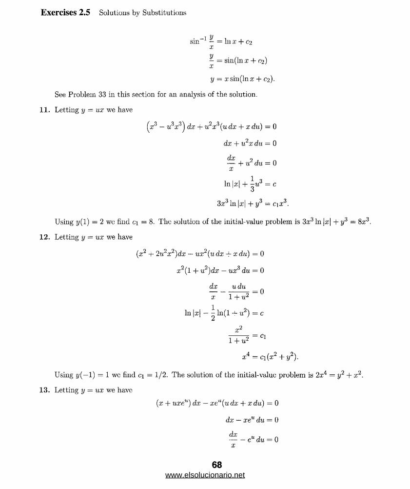
S il l ' — = 111 X + C2X
y . ,, N— = sm(in x + c'2 )
y = x sin (In x + C2 ).
See Problem 33 in this section for an analysis of the solution.
11. Letting y — ux we have
(x3 — w3x3) dx + u2x^(u dx + x du) — 0
dx + u2x du = 0
dx 9 , h u du = 0x
, , < 1 3 In |x| + -u = co
3.x3 In | x | + y3 = cix3.
Using y(l) = 2 we find c\ = 8. The solution of the initial-value problem is 3x:i In |x| + yi — 8x3.
12. Letting y — ux we have
(x2 4- 2u?x2)dx — ux2(udx -f xdu) = 0
x2(l + u2)dx — ux3 du = 0
dx u du
X 1 + u2
In |x[ — ^ ln(l -f u2) = c
Exercises 2.5 Solutions by Substitutions
x2= C l
1 + u2
X 4 - ci(x2 + y2).
Using y(—1) = 1 we find ci — 1/2. The solution of the initial-value problem is 2x4 = y2 + x2.
13. Letting y = ux we have
(x + uxeu) dx — xe“(u dx + x du) = 0
dx — xeu du = 0
dxzz _ eu du = 0x
68www.elsolucionario.net
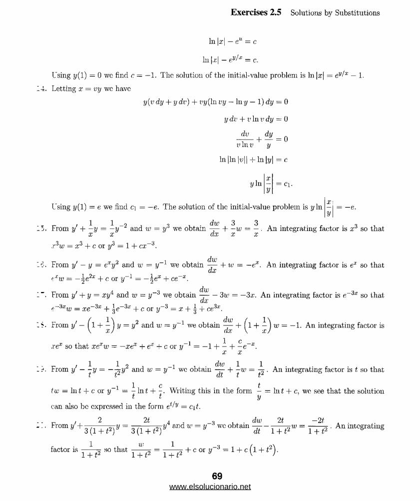
Exercises 2.5 Solutions by Substitutions
In |a*| — eu = c
In \x\ - eyfx = c.
Using y(l) = 0 wc find c = —1. The solution of the initial-value problem is In |.x[ = ey,lx — 1.
Letting x = vy we have
y(v dy + y dv) + vy(In vy — In y — 1) dy = 0
y dv + v In v dy — 0
dv dy + — = 0
v In v y
In | In I'l.'H + In |y| = c
y In = ci.
Using y(l) “ e we find ci = —e. The solution of the initial-value problem is y InX\
= — e.y
r- / 1 1 - o o . dw 3 3 . , oFrom y H— y — —y “ and w = y we obtain —— |- —w — — . An integrating factor is x so that
x' x' dx x x
x3w = x3 + c or t/3 = 1 + cx~A.
(I’ZUFrom y' — y — exy2 and w = y~l we obtain —— I- w = —ex. An integrating factor is ex so that
dxf:xw ~ — Ie2x + c. or y~l = — \ex + ce~x.
From y' + y = xy4 and w = we obtain — ■ — 3u> = —3x. An integrating factor is e~ix so thatdx
e~'ixw = xe~‘ix + + c or ;ty_a = x + ^ -i- cejx.
From y — y = y2 and w - y~l we obtain ^ + ^1 + w = —1. An integrating factor is
1 f*xex so that xexw = — xex + ex H- c or y-1 = — 1 + — + — e~x.
x x
/ 1 1 o , _i , . dto 1 1rrom y — -y = — -^y“ and w = y wc obtain — + —w = • An integrating factor is t so that
1 t- tw — In i -|- c or y~l — - Inf + Writing this in the form - = hit + c. we see that the solution
t t y ’
can also be expressed in the form e^y = cit.
/ 2 2t a , _■> . . dw 2t —21From y + 3 (1 + ^ */ = 3 (1 + t2)y ai W = V W° 0 am ~dt ~ l + f iW = TT f5 ’ mtcgratmg
-| * Xfactor is 80 that 1 ^ 2 = + c or y~* = 1 + c ( l + t2).
69www.elsolucionario.net

Exercises 2.5 Solutions by Substitutions
/ 2 3 4 . _o , . dw 6 9 . . . . . .21. Prom y -- y = — and w = y we obtain —— h —w = — . An integrating factor is x° so tha:
x x * ' dx x xz
x6w = —§x5 + c or y~3 = — §x_1 + cx~b. If y( 1) = ^ then c = ^ and y~3 = — fx -1 + ^ x -6.
dtxi. ■ 3 322. From if + y = y~1//2 and w = y3/2 we obtain — + -w = - . An integrating factor is e3x-/2 so tha:
fix z zeixl2w — (?x>2 + c or y3/2 = 1 + ce~iX/'2. If y(0) = 4 then c = 7 and ,(/}/2 = 1 + 7e~^xt2.
23. Let u = x -f'« + l so that du/dx = 1 + dy/dx. Then ^ — 1 = u2 or — —-x du = dx. Tlni-dx 1 + tr
tan-5 u = x + c or u = tan(x + c), and x + y + 1 = t.an(x + c) or y — tan(x + c) — x — 1.
24. Let u ~ x + y so that du/dx = 1 + dy/dx. Then ~ — 1 = ---- or u du = dx. Thus Aw,2 = x + .dx u
or u2 = 2x + ci. and (x + y)2 = 2x + cj.
25. Let u = x + y so that du/dx = 1 + dy/dx. Then ^ — 1 = tan2 u or cos2 udu = dx. Thu?\JfJU
^«+ |sin2u = x+c or 2«+sin2u = 4x+ei, and 2(x+y)+sin2(x+y) : 4x+ci or 2y+sin2(x+y) =
2x + ci.
26. Let u — x + y so that du/dx = 1 + dy/dx. Then — 1 = sin u o r-- — du = dx. Multiplyingctcc 1 sm *?/
1 sin bv (1 — sin if)/(1 — sin u) we have ---~— du = dx or (sec2 u — secu taiiu)du = dx. Thu-
cos u
tan u — sec u = x + c or tan(x + y) — sec(x + y) = x + c.
27. Let u = y — 2.x + 3 so that du/dx = dy/dx — 2. Then ^ + 2 = 2 + v/^ or ~t= du = dx. Thu-ax y w
2-y/w = x + c and 2^/y — 2x + 3 = x + c.
Let u = y — x + 5 so that du/dx =
—e~u = x + c and — ey~x+5 = x + c.
du28. Let u = y — x + 5 so that du/dx = dy/dx — 1. Then -— I- 1 = 1 + eu or e~udu = dx. Thi;.-
dx
ctu 129. Let u = x + y so that du/dx = 1 + dy/dx. Then --- 1 — cos u and----:-- du. = dx. Now
fix 1 + cos u
1 1 — cos u 1 — COS u O ----------------------------------------— — = CSC u — CSC u cot u1 + cos u 1 — cos2 u sin2 u
so we have f (csc2 u-c.sc u cot u)du = / dx and — cot w+csc u = x+c. Thus — cot(x+y) +csc(x+y) - |
x + c. Setting x = 0 and y = tt/4 we obtain c = a / 2 — 1 . The solution is
csc(x + y) - cot(x + y) = X + V2 — 1.
30. Let u = 3x + 2y so that du/dx = 3 + 2 dy/dx. Then ^ = 3+ — - = ~r~ and ^ du — d.i y ' Jl dx u + 2 u + 2 5 u + 6
Now bv long divisionu + 2 1 4
— ^ +5 u + 6 5 25u + 30
70www.elsolucionario.net
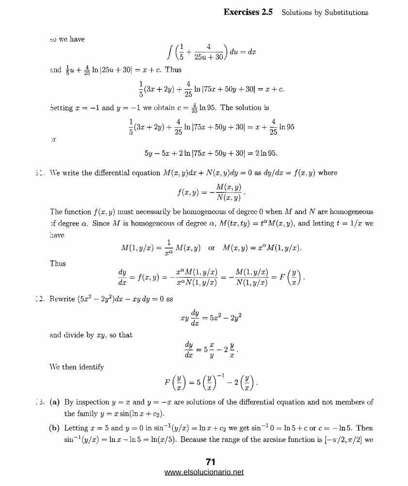
Exercises 2.5 Solutions by Substitutions
+ ~ ^ ) du = dx2 bu + 30,
~o we have
Idand ^ In |25?i + 30| = x + c. Thus
1 4~(3x + 2y) -f- — In |75x + 50y + 30| = x + c.D 2 d
Setting x = — 1 and y = — 1 we obtain c = ^ In 95. The solution is
1 4 4-(3a: + 2y) + — In \7ox + 50 y + 30| = x + — In 95o 25 2o
Jl'
5 y — 5x + 2 In |75.x + 50y + 30) = 2 In 95.
We write the differential equation M(x, y)dx + N(x, y)dy = 0 as dy/dx — f(x, y) where
f u v) =/ l ,W N(x. y) '
The function fix, y) must necessarily be homogeneous of degree 0 when M and N are homogeneous
jf degree a. Since M is homogeneous of degree a, M(tx7ty) = taM(x,y), and letting t = 1/x we
have
M (l,y/x) = M(x, y) or M (x, y) = xaM (1, y/x).
Thus
iy = f(T = rf*M{l,y/x) M (l,y/x) fy\
dx xaN(l,y/x) N(l,y/x) \x)
Rewrite (5:r2 — 2y2)dx — xy dy = 0 as
^ = 5*2-25,*dx
and divide by xy, so that
We then identify
dy „ x ^y -r = 5 - - 2 - .dx y x
X/ \x -)■X J(a) By inspection y = x and y = —x are solutions of the differential equation and not members of
the family y ~x sin (In a; + 02)-
(b) Letting x = 5 and y = 0 in sin-1 (y/x) = In x + 0 2 we get sin-1 0 = In 5 + c or c = — In 5. Then
sin-1 (y/x) = In x — In 5 = ln(,x/5). Because the range of the arcsine function is [—7r/2, tt/2] we
www.elsolucionario.net
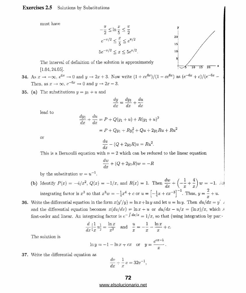
Exercises 2.5 Solutions by Substitutions
must have7T x -k
—— < ln - < —2 ~ 5 ~ 2
e-7r/2 < - < e*-/2 5
5e_ ^/2 < a: < 5ew/2.
The interval of definition of the solution is approximately
[1.04,24.05].
34. As x —*• —oc. —► 0 and y —*• 2x + 3. Now write (1 -I- ce6*)/(l — ce6x) as (e~bx + c)/(e~6x —
Then, as x —> oo, (?~fxT —> 0 and y —> 2x — 3.
35. (a) The substitutions y — yi + u and
dy _ clyi | du
dx dx dx
lead to
+ y- = P + Q(tli + u) + R(yi + u)2dx dx
= P + Qy\ -j- Ry'i + Qu + 2y\ Ru + Ru2
or
~ ~ { Q + 2yi R)u = Ru2. dx
This is a Bernoulli equation with n = 2 which can be reduced to the linear equation
div—— h (Q + 2y\ R)tv — —R dx
bv the substitution w = u
(b) Identify P(x) = -4/x2, Q{x) = - 1/x, and R(x) = 1. Then ~ -f - + - )w = - 1. .-j
-l
dw
dx
■\x + cx~3
1 4
x x,- l 2
. Thus, y ~ — h u. x
integrating factor is a’3 so that x^w = —|x4 + e or u =
36. Write the differential equation in the form x(y'/y) — Inx+Iny mid let u — lny. Then du/dx = y' j
and the differential equation becomes x(du/dx) = lnx -j- u or du/dx — u/x = (lnx)/x. which j
first-order and linear. An integrating factor is e~J dx/a: = 1/x. so that (using integration by par:-
d_
dx
lnx uu ! = —7T and - =
x J r/ x
1 lnx
x x+ c.
The solution is
In y = — 1 — In x -r cx or y =X
37. Write the differential equation as
- - v = 32vdx x
72www.elsolucionario.net

Exercises 2.5 Solutions by Substitutions
; ::d let u = v2 or v = u1 . Thendv _ 1 _xj 2 du
dx 2 dx '
.-.lid substituting into the differential equation, wc have
1 i / o dlli 1 i / o -1/9 d<u 2-u — I- - u < = 32u /_ or — + - u = 64.2 dx x dx x
The latter differential equation is linear with integrating factor cJ 'x dx = x2. so
-y- [x2,u] — 64x2 dx
-.nd9 64 o 0 64 c
x"u = — x° + c or v~ = — x + —r3 3 :rJ
".'. rite the differential equation as dPjdt — aP = —bP2 and let u = P 1 or P = u
dp _9 du— = — u — , dt dt
}.::A substituting into the differential equation, wc have
_2 du _9 du—u —-- au = —bit " or — + au = b.
dt dt
The latter differential equation is linear with integrating factor eJ 11 dt — cat, so
d r .a t„ , 1 _ t ^ a i
:id
\e m = be dt ■- J
eatu = - eal — c a
ea lp ~ I = b eat + c a
P ~ l = - + ce- at a
P = 1b/a + ce at b-\-C\e~al
-1. Then
73www.elsolucionario.net
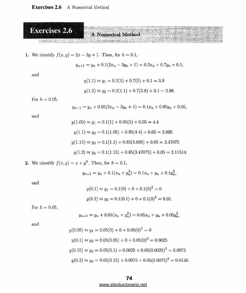
Exercises 2.6 A Numerical Method
■'h Num erical-M ethod' w, kc: ..
' "r -
-*•£,' ' -\-5 .,S J s C„, „„ . „ „ , „„ „1 . ,J'.'i :* \' w" ; ......I ......v'c. 't,„ %y' ; /
1. We identify f(x, y) = 2x — ?>y + 1. Then, for h = 0.1,
Vn+1 = Vn 4" 0.1 (2.x7l 3y;; + 1) = 0.2xw + 0.7y-a ~\~ 0.1,
and
For h = 0.05.
and
2/(l.l) » yi = 0.2(1) 4- 0.7(5) + 0.1 = 3.8
y( 1.2) « y2 = 0.2(1.1) + 0.7(3.8) + 0.1 = 2.98.
Vn—i — Vn + 0.05(2.rn — 3 yn + 1) = 0. l.xn + 0.85'//n + 0.05,
y( 1.05) « yi = 0.1(1) + 0.85(5) + 0.05 = 4.4
y (l.1) » 2/2 = 0.1(1.05) + 0.85(4.4) + 0.05 = 3.895
2/(1.15) « yA = O .l(l.l) + 0.85(3.895) + 0.05 = 3.47075
2/(1.2) » y4 = 0.1(1.15) + 0.85(3.47075) + 0.05 = 3.11514.
2. We identify f(x,y) = x + y2. Then, for h = 0.1,
V n + l = V n + 0.1(xn + yl) = 0.1 Xn + Vn + O .lt /^ ,
and
2/(0.1) « 2/i = 0.1(0) + 0 + 0.1(0)2 = 0 y(0.2) « 2/2 = O.l(O.l) + 0 4- 0.1(0)2 = 0.01.
For h = 0.05.
and
yn+1 = yn + 0.05(.i‘n + yi) = 0.05a; + yn + 0.05y2,
2/(0.05) « yi = 0.05(0) + 0 + 0.05(0)2 = 0
y(0.1) « 2/2 = 0.05(0.05) + 0 + 0.05(0)2 = 0.0025
2/(0.15) « 2/3 = 0.05(0.1) + 0.0025 + 0.05(0.0025)2 = 0.0075
2/(0.2) » y4 = 0.05(0.15) + 0.0075 4- 0.05(0.0075)2 = 0.0150.
74www.elsolucionario.net
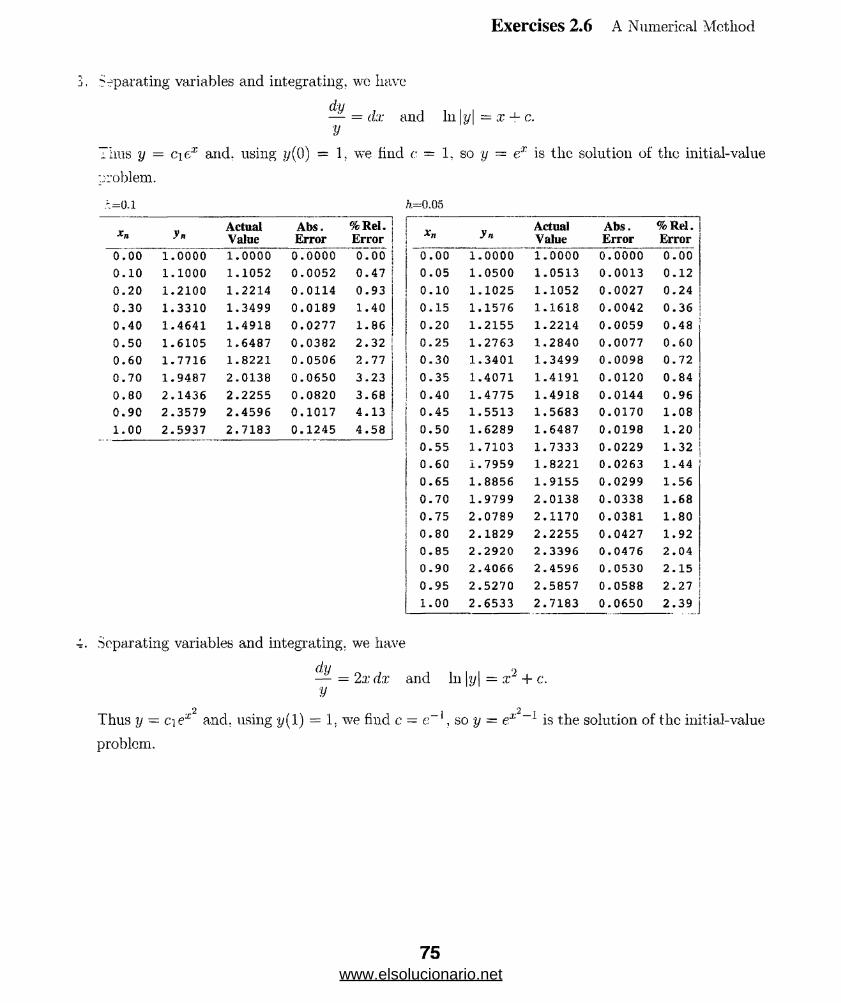
Exercises 2.6 A Numerical Method
= dx and In I y\ = x H- c.
separating variables and integrating, we have
dy
y
rims y = C[ cx and. using y(0) = 1, we find c = 1, so y = ex is the solution of the initial-value
problem.
/:=0.1 ft— 0.05
0.000. 100 . 20
0.30
0.40
0.50
60
70
80
90
1.00
ActualValue
Abs.Error
1.00001.10001.21001.3310
1.4641
1.6105
1.7716
1.9487
2.1436
2.3579
2.5937
1.00001.1052
1.2214
1.3499
1.4918
1.6487
1.8221
2.0138
2.2255
2.4596
2.7183
%ReI.Error
0.00000.0052
0.0114
0.0189
0.0277
0.0382
0.0506
0.0650
0.0820
0.1017
0.1245
0.000.47
0.93
1.40
1.862.32
2.77
3.23
3.68
4.13
4.58
*71 yn ActualValue
Abs.Error
% Rel. Error
0.00 1.0000 1.0000 0.0000 0.00
0.05 1.0500 1.0513 0.0013 0.12
0.10 1.1025 1.1052 0.0027 0.24
0.15 1.1576 1.1618 0.0042 0.36
0.20 1.2155 1.2214 0.0059 0.48
0.25 1.2763 1.2840 0.0077 0.60
0.30 1.3401 1.3499 0.0098 0.72
0.35 1.4071 1.4191 0.0120 0.84
0.40 1.4775 1.4918 0.0144 0.96
0.45 1.5513 1.5683 0.0170 1.08
0.50 1.6289 1.6487 0.0198 1.20
0.55 1.7103 1.7333 0.0229 1.32
0.60 1.7959 1.8221 0.0263 1.44
0.65 1.8856 1.9155 0.0299 1.56
0.70 1.9799 2.0138 0.0338 1.68
0.75 2.0789 2.1170 0.0381 1.80
o . 00 o 2 .1829 2.2255 0.0427 1.92
0.85 2.2920 2.3396 0.0476 2.04
0.90 2.4066 2.4596 0.0530 2.15
0.95 2.5270 2.5857 0.0588 2.27
1.00 2.6533 2.7183 0.0650 2.39
4. Separating variables and integrating, we have
— = 2x dx and In \y\ — x2 + c.y
Thus y — ciex'2 and. using y(l) = 1. we find c — e~l , so y = e**-1 is the solution of the initial-value
problem.
75www.elsolucionario.net
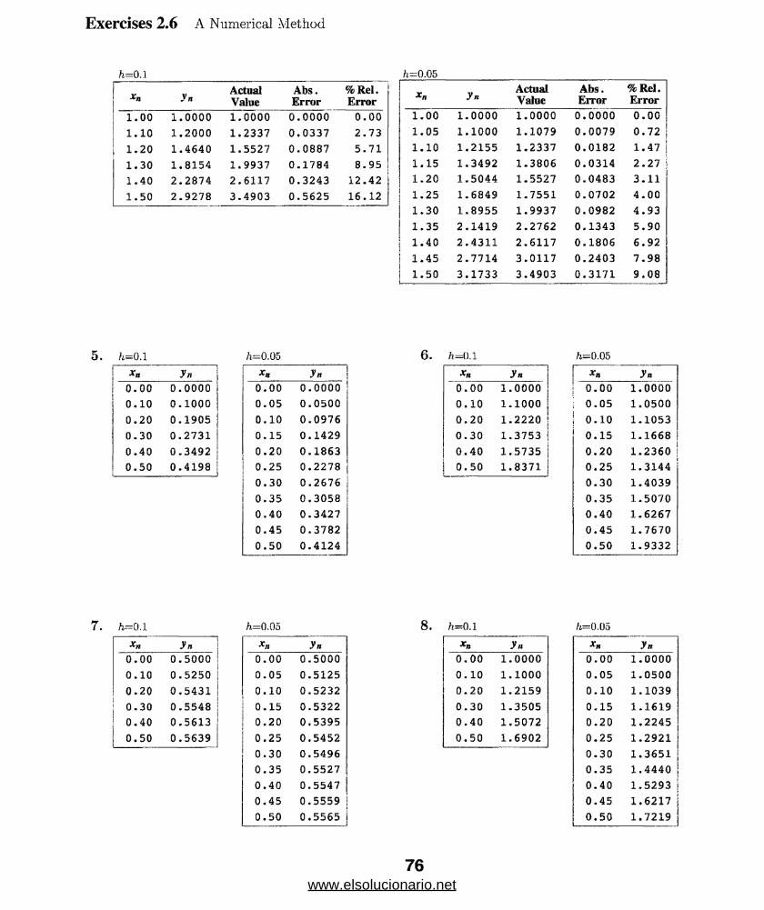
Exercises 2.6 A Numerical Method
h=0.1xn yn Actual
ValueAbs.Error
%ReI.Error
1.00 1.0000 1.0000 0,0000 0,00
1.10 1,2000 1.2337 0.0337 2.73
1.20 1.4640 1,5527 0,0887 5.71
1,30 1.8154 1.9937 0.1784 8.95
1.40 2.2874 2.6117 0.3243 12.42
1.50 2.9278 3.4903 0.5625 16.12
fr—0.05
Xn yn ActualValue
Abs.Error
% ReJ. Error
1.00 1.0000 1.0000 0.0000 0.00
1.05 1.1000 1.1079 0.0079 0.72
1.10 1,2155 1.2337 0.0182 1,47
1.15 1.3492 1.3806 0.0314 2.27
1.20 1.5044 1.5527 0.0483 3.11
1.25 1.6849 1.7551 0.0702 4.00
1.30 1.8955 1.9937 0.0982 4.93
1.35 2.1419 2.2762 0.1343 5.90
1.40 2.4311 2.6117 0.1806 6.92
1.45 2.7714 3.0117 0.2403 7,98
1.50 3.1733 3.4903 0.3171 9.08
5. h=0.1 /i=0.05
Xn y»0.00 0.0000
0.10 0.1000
0.20 0.1905
0.30 0.2731
0.40 0.3492
0.50 0.4198
Xn yn
oo«o
0 .0000
0.05 0.0500
o
«—i
o
0 ,0976
0.15 0.1429
0.20 0,1863
0.25 0.2278
0.30 0.2676
0.35 0.3058
0.40 0.3427
0.45 0.3782
oo
0 .4124
/i—0.1 h = 0.05
Xn yn
ooo
0 ,5000
0.10 0,5250
0,20 0.5431
0.30 0.5548
oO
0.5613
0.50 0.5639
Xn yn0.00 0.5000
0.05 0.5125
0.10 0.5232
0.15 0.5322
0.20 0.5395
0.25 0.5452
0.30 0.5496
0,35 0.5527
0.40 0.5547
0.45 0.5559
0.50 0,5565
6. /i=o.i ft=0.05
yn
ooo
1,0000
0.10 1.1000
0.20 1,2220
0.30 1.3753
0.40 1.5735
oino
1.8371
8 . h = o.i
Xn yn0,00 1.0000
o i—1
o 1.1000
0.20 1.2159
0.30 1.3505
0.40 1.5072
0.50 1.6902
i Xn yn; o .oo 1.0000
i 0 .05 1.0500
0.10 1.1053
0.15 1.1668
0.20 1.2360
0.25 1.3144
0.30 1.4039
0.35 1.5070
0.40 1.6267
0.45 1.7670
0.50 1.9332
^=0.05
Xn y n0.00 1.0000
0.05 1.0500
0.10 1.1039
0.15 1.1619
0.20 1.2245
0.25 1.2921
0.30 1.3651
0.35 1.4440
0.40 1.5293
0.45 1.6217
0.50 1.7219
76www.elsolucionario.net
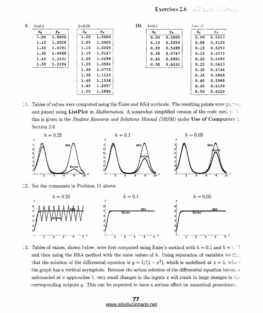
9. ft=o.i
Jn| 1.00 1.0000
: 1.10 1.0000
1.20 1.0191
1.30 1.0588
1.40 1.1231
1.50 1.2194
h = o m
1 . 0 0 1.05
1.10 1.15
1.20 1.25
1.30
1.35
1.40
1.45
1.50
10.y*1.0000
1.00001.0049
1.0147
1.0298
1.0506
1.0775
1.1115
1.1538
1.2057
1.2696
Exercises 2.6 . .1..
ft=0.1 h=0.joyn v»
0.00 0.5000 0.00 0.500D
0.10 0.5250 0.05 0.5125
0.20 0.5499 0.10 0.5250
0.30 0.5747 0.15 0.5375
o
.O
0.5991 0.20 0.5499
0.50 0.6231 0.25 0.5623
0.30
0.35
0.40
0.45
0.50
0.5746
0.5868
0.5989
0.6109
0.6228
. 1. Tables of values were computed using the Euler and RK4 methods. The resulting points were pic:
and joined using ListPlot in Mathematica. A somewhat simplified version of the code used
this is given in the Student Resource and Solutions Manual (SRSM) under Use of Computers
Section 2.6.
h = 0,1h = 0.25 h = 0.05
2. See the comments in Problem 11 above.
h = 0.25 h = 0.05
"EuleRK4
E u le rRK4
1 2 3 4 5
.3. Tables of values, shown below, were first computed using Euler’s method with h = 0.1 and h = 0. ’
and then using the RK4 method with the same values of h. Using separation of variables we nr.
that the solution of the differential equation is y = 1/(1 — a;2), which is undefined at x = 1. whd
the graph has a vertical asymptote. Because the actual solution of the differential equation becoir.-
unbounded at x approaches 1, very small changes in the inputs x will result in large changes in
corresponding outputs y. This can be expected to have a serious effect on numerical procedures.
77www.elsolucionario.net
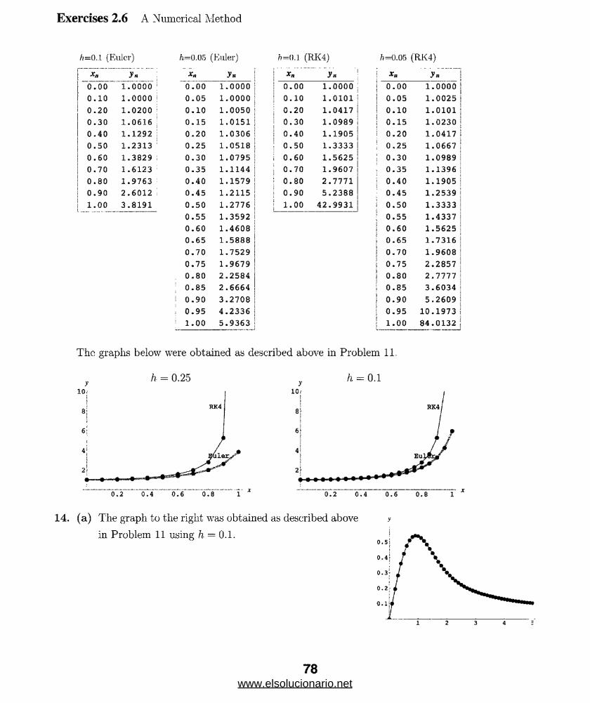
Exercises 2.6 A Numerical Method
=0.1 (Euler)
** yn
ft—0.05 (Euler)
Xn yn
/?—().! (RK4)
Xn yn
ft =0.05 (RK4)
Xa yn
O O o 1.0000 1 0.00 1*0000 | 0.00 1.0000
Ooo
1.0000o o 1.0000 ! 0 .05 1.0000 | 0.10 1.0101 o o U1 1.0025
0.20 1.0200 ! 0 .10 1.0050 0.20 1.0417 0.10 1.0101
oCT)o
1.0616 0.15 1.0151 0.30 1.0989 0.15 1.0230
oo
1.1292 0.20 1.0306 0.40 1.1905 j 0 .20 1.0417
0.50 1.2313 1 0.25 1.0518 0.50 1.3333 ! 0.25 1.0667
oVOo
1.3829 i 0.30 1.0795 j 0.60 1.5625 ! 0.30 1.0989
0,70 1.6123 : 0.35 1.1144 | 0.70 1.9607 j 0.35 1.1396
0.80 1.9763 : 0.40 1.1579 o 00 o 2.7771oO
1.1905
0.90 2.6012 I 0.45 1.2115 j 0.90 5.2388 • 0.45 1.2539
1.00 3.8191 0.50 1.2776 o o 42.9931 j 0.50 1.3333
0.55 1.3592 | 0.55 1.4337
0.60 1.4608 | 0.60 1.5625
0.65 1.5888 j 0.65 1.7316
0.70 1.7529 j 0.70 1.9608
0.75 1.9679 j 0.75 2.2857
. 0.80 2.2584 | 0.80 2.7777
; 0.85 2.6664 j 0.85 3.6034
i 0 .90 3.2708 | 0.90 5.2609
0.95 4.2336 | 0.95 10.1973
| 1.00 5.9363 ! 1 . 0 0 84.0132
The graphs below were obtained as described above in Problem 11.
h = 0.25 y h = 0.1
14. (a) The graph to the right was obtained as described above >•
in Problem 11 using h — 0.1.0 . 5 {
0 . 4 j
0 . 3 -
0.2-
0.1
78www.elsolucionario.net

Chapter 2 in Review
(b) Writing the differential equation in the form 1/ + 2xy = 1 we see that an integrating factor is
..... ~2, / 2 xdx = ex-_ SQ
(I 2 2 -rlex V\ =dx
and.,2 t'x i l , _..,2
dt + ce .y = (-*2 f JO
This solution can also be expressed in terms of the inverse error function as
y = e“x"erfi(a:) + ce_ar.
Letting x = 0 and y(0) — 0 we find c = 0. so the solution of the initial-value problem is
J2 l‘x ,2y = e x e1 dt = —y e z erfi(.r).
(c) Using either F indRoot in Mathematica or f so lve in Maple we see that y'(x) = 0 when
x = 0.924139. Since //(0.924139) 0.541044. we see from the graph in part (a) that
(0.924139.0.541044) is a relative maximum. Now. using the substitution u = —t in the in
tegral below, we have
y(—x) = e~<K~x j dt = a~x j e*--^ (—du) = —e~x J du du = —y(x).
Thus. y(x) is an odd function and (—0.924139. —0.541044) is a relative minimum.
Writing the differential equation in the form y' = k(y + A/k) we see that the critical point —A/k
is a repeller for k > 0 and an attractor for k < 0.
1. Separating variables and integrating we have
^ = A dxy x
In y = 4 In x -r c — In a’4 + c
y = cix4.
We see that when x = 0. y = 0. so the initial-value problem lias an infinite number of solutions for
v = 0 and no solutions for k ^ 0.
:. True; y = k-2 /k-i is always a solution for k\ 0.
79www.elsolucionario.net

Chapter 2 in Review
4. True; writing the differential equation as a\{x)dy + (i2 (x)ydx = 0 and separating variables yield-
7. When n is odd, xn < 0 for x < 0 and xn > 0 for x > 0. In this case 0 is unstable. When n is eve:
xn > 0 for x' < 0 and for x > 0. In this case 0 is semi-stable.
When n is odd, —xn > 0 for x < 0 and —xn < 0 for x > 0. In this case 0 is asymptotically stab’:
When n is even, —xn < 0 for x < 0 and for x > 0. In this case 0 is semi-stable.
8. Using a CAS we find that the zero of / occurs at approximately P = 1.3214. From the gra; ...
we observe that dPjdt > 0 for P < 1.3214 and dPjdt < 0 for P > 1.3214. so P = 1.3214 is : i
asymptotically stable critical point. Thus, lim.*-^ P(t) = 1.3214.
9. ............ v..............
5. s?
6. ^ = y(y - 2f(y - 4)
10. (a) linear in y. homogeneous, exact
(c) separable, exact, linear in x and y
(e) separable
(g) linear in x
(i) Bernoulli
(b) linear in x
(d) Bernoulli in x
(f) separable, linear in x, Bernoulli
(h) homogeneous
(j) homogeneous, exact, Bernoulli
(k) linear in x and y. exact, separable, homogeneous
(1) exact, lineai' in y (m) homogeneous
(n) separable
11. Separating variables and using the identity c.os2x = 5(1 + cos 2a:), we have
and
80www.elsolucionario.net
Chapter 2 in Review
2x + sin 2x = 2 In (jj2 + l) + c.
12. Write the differential equation in the form
y In - dx = ( x In — — v I dy.' y \ y ' J
This is a homogeneous equation, so let x = uy. Then dx = udy + y du and the differential equation
becomes
y In u(u dy + y du) — (■uy In u — y) dy or y In u du = —dy.
Separating variables, we obtain
lr iu du = - —V
a hi \ u\ — u. = — In |y| + c
-In
13. The differential equation
y
.r(ln.x — In y) — x = —yin |y| + cy.
dy 2 3.x-2 _2V = ~ 7 -— r r vdx 6x + 1' 6x + 1
is Bernoulli. Using w = if’, we obtain the linear equation
dw 6 9x2 — I- ----- « ■ =
dx 6a; + 1 6x -4- 1
An integrating factor is Gx + 1. so
4- [(6* + l)w] = -9.x2,dx
3a"3 c. w = ~ ~---r +
6.x + 1 6.x + 1 ' and
(Qx + l)y^ = —3.x'3 + c.
Note: The differential equation is also exact.)
14. Write the differential equation in the form (3y2 + 2x)dx + (4y2 + 6xy)dy = 0. Letting M = 3y2 + 2x
and N = 4y2 4- 6xy wc see that My = 6y = Nx, so the differential equation is exact. From
fx = 3y2 + 2x we obtain / = 3xy2 + x2 + h(y). Then f y = 6xy + h'(y) = 4y2 + 6xy and h'(y) = 4y2
50 h(y) = |y3. A one-parameter family of solutions is
3xy2 -f x2 + ^y’3 = c.O
81www.elsolucionario.net
Chapter 2 in Review
15. Write the equation in the form
An integrating factor is eln< = t, so
dQ 1 o
a + -t Q = t l n t
| [ tQ i= t4ln(
tQ = -t !ii t + cZo 0
and
Q = - k t i+ \t lh u + -f
16. Letting u = 2x + y + 1 we have
— = • ? + <f y .
dx dx ’
and so the given differential equation is transformed into
( du , du 2 u +1“U “2j = 1 or Tx = — ■Separating variables and integrating we get
du = dx2u 1
1 1 1
2 2 2 u + 1du = dx
•u - ^ In |2u + 1| = x + c
2 u — In |2 u + 1| —2x + c\.
Resubstituting for u gives the solution
4x + 2y + 2 — In \4x -j- 2y + 3| = 2x + c\
or
2x + 2 y + 2 — In |4rc + 2 y —1— 3| = ci-
17. Write the equation in the form
dy . 8x 2x
dx ' x2 + 4^ x2 + 4'
An integrating factor is (a.’2 + 4 , so
;§ [ ( :,;’ + 4 ) \ ] = 2 ^ + 4) 3
82www.elsolucionario.net
Chapter 2 in Review
>.nd
y
(;X2 + 4 4 y = 2 (x‘2 + 4)4 + c
= \ + c(x* + 4) - \4
1. letting M = 2r2 cos 0 sin 0 + r cos 0 and N = 4r + sin 6* — 2r cos2 0 we see that Mr = 4r cos 0 sin 0 +
::>s0 = j¥(9, so the differential equation is cxact. From fo = 2 r 2 cos 6 sin 9 + r cos 9 we obtain
* = —r2 cos2 0 + r sin 9 -j- /i(r). Then f r — —2r cos2 # + sin 0 + ///(7') = 4 r + sin 9 — 2r cos2 0 and
:.' r) = 4r so /i(r) = 2r2. The solution is
—r2 cos2 0 + r sin 9 + 2r2 = c.
*. The differential equation has the form (d/dx) [(sina:)y] = 0. Integrating, we have (sin x)y = c or
. = c/ sinx. The initial condition implies c = — 2sin(77r/6) = 1. Thus, y — 1/ sin a:, where the
interval 7r < X < 2tt is chosen to include x = 7n/6.
. separating variables and integrating we have
= -2(t + 1) dty2
- i = -(« + l)2 + cy
y ~ z/ t 'iL i— > where ~c = Cl-(t + ly + ci
The initial condition y(0) — —| implies ci = — 9, so a solution of the initial-value problem is
1 1
V (i H-l)2 -9 01 V *2 + 2*_ s ’
"•here — 4 < * < 2.
.. i a) For y < 0. y/y is not a real number.
i b) Separating variables and integrating we have
dy , . . _—— = dx and 2 /y = x + c.
Letting y(xo) = yo we get c = 2v/yo - x0, so that
2\py = :r + 2v/yo — xq and y = ^{x + 2^/y^ - xo)2.
Since ^Jy > 0 for y ^ 0. we see that dy/dx = \(x + 2 /yo ~ -o) must be positive. Thus; the
interval on which the solution is defined is (xq — 2y/yo, oo).
83www.elsolucionario.net
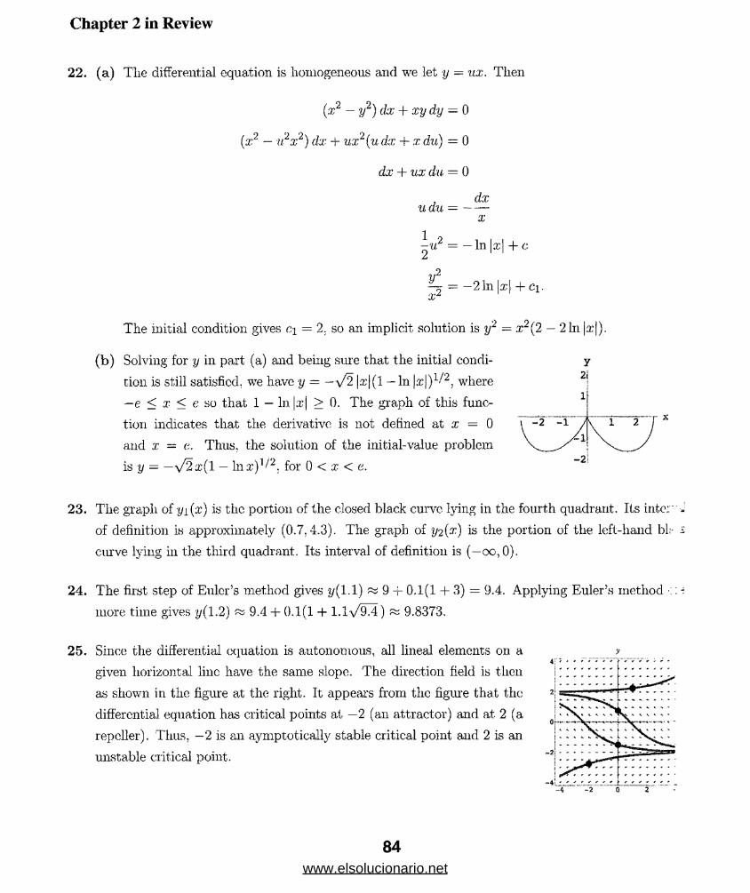
Chapter 2 in Review
22. (a) The differential equation is homogeneous and we let y - ux. Then
(x2 - y2) dx + xy dy = 0
(a:;2 ■ u2x2) dx + ux1 (u dx + x du) = 0
dx + ux du = 0
dxudu = ---
x
^ u2 = - In |x| + c
y2= —2 In |xj + ci.
The initial condition gives ci = 2. so an implicit solution is y1
( b ) Solving for y in part (a) and being sure that the initial condi
tion is still satisfied, we have y — — \/2 |.x’|(l — In \x\)1!2, where
—e < x < c so that 1 — In |rcj > 0. The graph of this func
tion indicates that the derivative is not defined at x = 0
and x — e. Thus, the solution of the initial-value problem
is y = —y/2x(l — In a:)1/2, for 0 < x < e.
23. The graph of yi(x) is the portion of the closed black curve lying in the fourth quadrant. Its inter'' J
of definition is approximately (0.7.4.3). The graph of JJ2 {^) is the portion of the left-hand bl;- i
curve lying in the third quadrant. Its interval of definition is (—oo,0).
24. The first step of Euler’s method gives y (l.l) ~ 9 -r 0.1(1 + 3) = 9.4. Applying Euler’s method :: ■?
more time gives y(1.2) ~ 9.4 + 0.1(1 + l.l\/9^4) ~ 9.8373.
25. Since the differential equation is autonomous, all lineal elements on a
given horizontal line have the same slope. The direction field is then
as shown in the figure at the right. It appears from the figure that the
differential equation has critical points at —2 (an attractor) and at 2 (a
repeller). Thus, —2 is an aymptotically stable critical point and 2 is an
unstable critical point.
= x2(2 - 21n|x|).
84www.elsolucionario.net
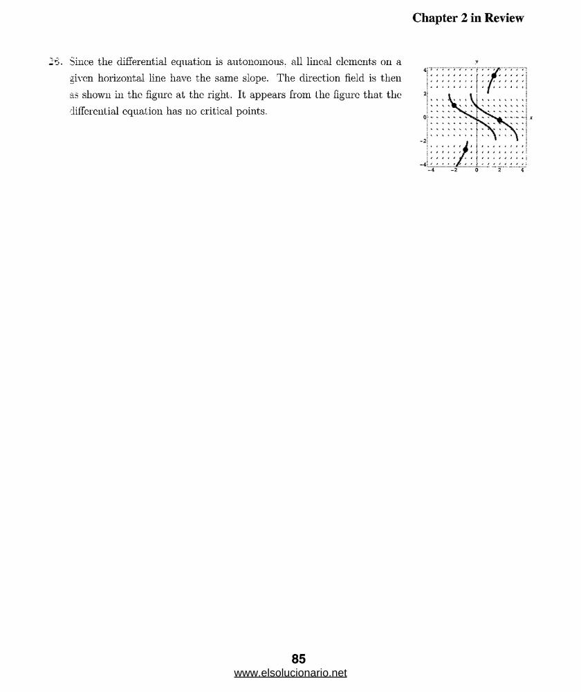
Chapter 2 in Review
2t>. Since the differential equation is autonomous, all lineal elements on a
given horizontal line have the same slope. The direction field is then
as shown in the figure at the right. It appears from the figure that the
differential equation has 110 critical points.
- 4 - 2 0 2 4
v
85www.elsolucionario.net

3 Modeling with First-Order Differential Equations
lin e a r M odels: v. •/
1. Let P = P(t) be the population at time t. and Po the initial population. From dP/dt — kF
obtain P — P^eM. Using P{5) = 2Po w c find k = | ln2 and P = Poe(ln2)|t/'5. Setting P(t) =
we have 3 = gO112)*/0. so
, o O 2)* , 5 In 3In3 = — -— and t = — « r.9 years.
5 In 2
Setting P(t) = 4P0 wc have 4 = e ^ 2)*/5, so
, , (In 2)*In 4 = — -— and t fa 10 vears.
5
2. From Problem 1 the growth constant is k = i In 2. Then P = P0e 1,/5 ln2'f and 10,000 = Poe 3/'
Solving for Po we get Pq - 10,000e“ ^ / 5 ,n2 = 6,597.5. Now
P(10) = poe(1/5)(|n2)(i°) = 0>597i5e2in2 = 4Fq = 26,390.
The rate at which the population is growing is
P '(10) = fcP(10) = ^(ln2)26,390 = 3658 persons/vear.5
3. Let P = P(t) be the population at time t. Then dP/dt, = kP and P = cekt. From P (0) = c =
we see that P = 500efct. Since 15% of 500 is 75, we have P (10) = 500elofc = 575. Solving for ;
get k = In ^ In 1.15. When t = 30.
P(30) = 500e(1/lo)(ln 1,15)30 = 500e3 In1-15 = 760 years
and
P'(S0) = kP(30) = -^(ln 1.15)760 = 10.62 persons/year.
4. Let P = P(t) be bacteria population at time t and Po the initial number. From dP/dt = kF
obtain P = Poe**. Using P(3) = 400 and P(10) = 2000 we find 400 = Poe3fc or ek = (400/P
From P(10) = 2000 we then have 2000 = Poelofe = Po(400/P())10'/3, so
2000 _ _ 7 /3 , „ ( 2000 \ ~ 3/7 ^——177777 = Pn and Po = (-- 7777z ) ~ 201.40010/ j 0 V40010/3/
86
www.elsolucionario.net

Exercises 3.1 Linear Models
le t A = A(t) be the amount of lead present at time t. From dA/dt = kA and .4 (0) = 1 we obtain
4 _ eU Using A(3.3) = 1/2 wc find k = ^ ln (l/2). When 90% of the lead has decayed, 0.1 grams
“'ill remain. Setting A(t) = 0.1 we have (-/(1-/ -i)ln(1/2) — 0.1, so
* , 1 i , 3.3In0.1— In - — In 0.1 and t = —-—r—- ps 10.96 hours.3.3 2 hi(l/2)
lot A = A(t) be the amount present at time t. From dA/dt = kA and ,4(0) = 100 we obtain
- 100ett. Using ,4(6) - 97 we find k = J hi 0.97. Then .4(24) = 100e(i/6)(hl°-97)24 = 100(0.97)4 ss
iS.o mg.
Writing A(t) = 50 in Problem 6 we obtain 50 = lOOe*'*, so
i 1 i In (l/2)kt — m - and t = . . .——— ~ 136.5 hours.
2 (1/6) In 0.97
* a) The solution of dA/dt = kA is A(t) = Aoeki. Letting A = ^Aq and solving for t we obtain the
half-life T = - (In2)/k.
b ) Since k = —(In2)/'I7 we have
A(t) = A oe-^W 7 = A02~t/T.
c) Writing |4o ~ Aq‘2~L/"1 as 2-3 = and solving for t we get t = 3T. Thus, an initial
amount Aq will decay to | 4 q in three half-lives.
* !:•: 7 = I(t) be the intensity, t the thickness, and 7(0) = 7o- If dl/dt = k l and 7(3) = 0.257o, then
: = hek\ k = \ In 0.25, and 7(15) = 0.000987o.
7:::n dS/dt — rS wc obtain S — Sqc'1 where 5(0) — Sq.
a) If 5b = $5000 and r = 5.75% then 5(5) = $6665.45.
b) If S(t) =$10,000 then t = 12 years.
:« 5 « $6651.82
-_"'ime that A = Aoekt and k = -0.00012378. If .4(<) = 0.145-4o then t ^15,600 years.
1. 7:.m Example 3 in the text, the amount of carbon present at time t is A(t) = ,4ne_0'000123'8*.
L-::ing t — 660 and solving for Aq we have A(660) = 4 0e-0 000l237(660) = 0.92 1553 4o- Thus,
■::: roxirnately 92% of the original amount of C-14 remained in the doth as of 1988.
-.“ time that dT/dt = k(T— 10) so that T = 10 + ce^. If T(0) = 70° and T (l/2) = 50° then c = 60
k = 21n(2/3) so that T( 1) = 36.67°. If T(t) = 15° then t = 3.06minutes.
--“ ■.une that dT/dt = k(T — 5) so that T = 5 + cekt. If T(l) = 55° and T(5) = 30° then k = — j In 2
1 c = 59.4611 so that T(0) = 64.4611°.
87www.elsolucionario.net
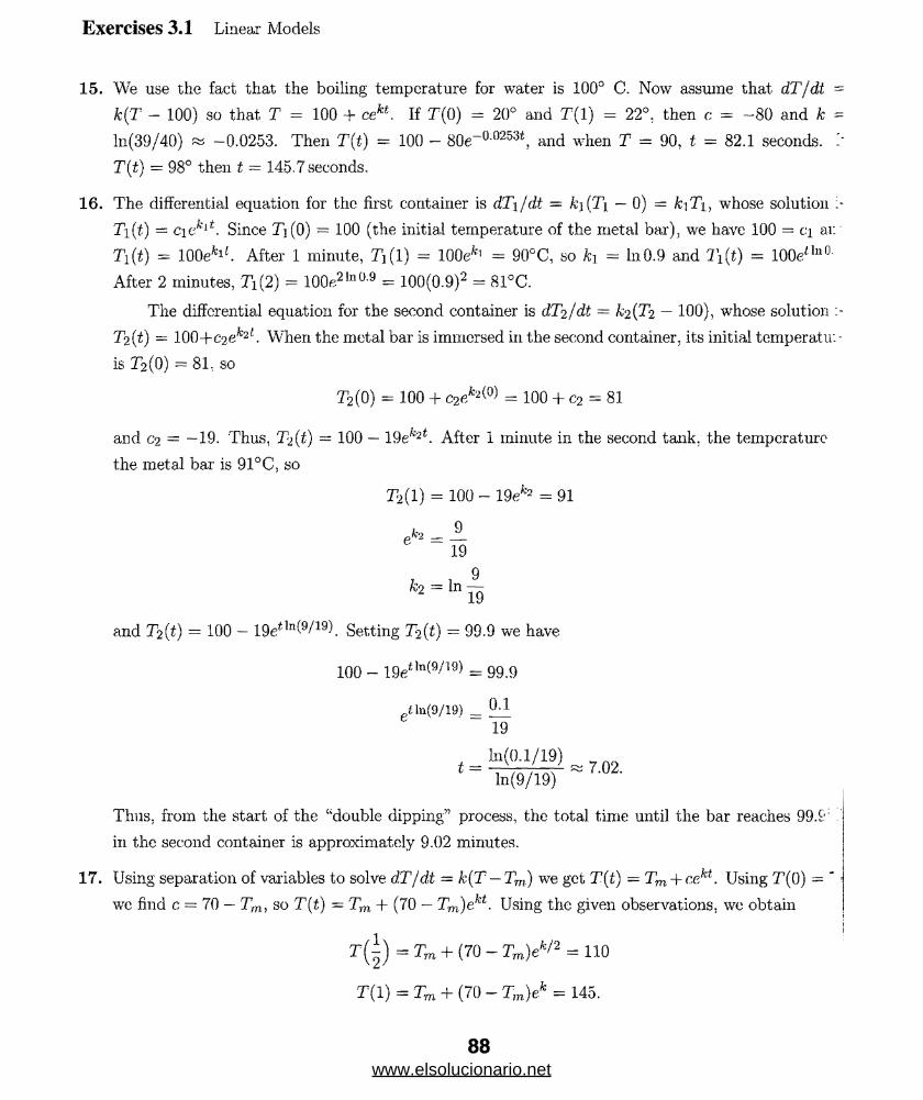
Exercises 3.1 Linear Models
15. We use the fact that the boiling temperature for water is 100° C. Now assume that dT/dt =
k(T - 100) so that T = 100 + cekt. If T(0) = 20° and T(l) = 22°, then c = -80 and k =
ln(39/40) —0.0253. Then T(t) = 100 — 80e-0 0253t, and when T = 90, t = 82.1 seconds.
T(t) = 98° then t = 145.7 seconds.
16. The differential equation for the first container is dT\jdt = k](Ti — 0) = k\Ti, whose solution
Ti(t) = cieklt. Since Xj (0) = 100 (the initial temperature of the metal bar), we have 100 - c\ an
Ti(t) -- 100efclf. After 1 minute, T i(l) = lOOe*1 = 90°C, so h = In0.9 and l\(t) = 100e'hl°
After 2 minutes, T\(2) = 100e21ll° 9 = 100(0.9)2 = 81°C.
The differential equation for the second container is dT^jdt = hi (Th — 100), whose solution
T2(t) - 100+C2.efc2<. When the metal bar is immersed in the second container, its initial temperatir. -
is T2(0) = 81, so
T2(0) = 100 + c2ek' ^ = 100 + c2 = 81
and e2 = —19. Thus, T2(i) = 100 — I9ek2t. After 1 minute in the second tank, the temperature
the metal bar is 91°C. so
jT2( 1) = 100 - 19e*2 = 91
efca = JL6 19
and 72(f) = 100 — 19ef lnC9/19). Setting T^it) - 99.9 we have
100 - 19enn(9/19) = 99.9
f 111(9/ 19) _~ 19
t = M E M . 7 ,0 2 .ln(9/19)
Thus, from the start of the “double dipping” process, the total time until the bar reaches 99.9;
in the second container is approximately 9.02 minutes.
17. Using separation of variables to solve dT/dt — k(T — Trn) we get T(t) - Tm + cekt. Using T(0) - '
we find c = 70 — Tm, so T(t) = Tm + (70 — Tm)ekt. Using the given observations, we obtain
r ( i ) = Tm + (70 - Tm)ekl2 = 110 T ( l ) = T m + ( 7 0 - T m)e* = 145.
88www.elsolucionario.net
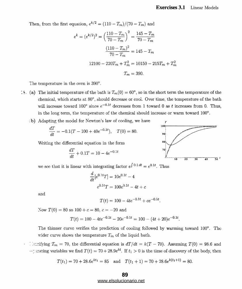
Exercises 3.1 Linear Models
Then, from the first equation, ek/2 — (110 — Tm)/{70 — Tm) and
110 -Tm
70 -Tm
(110 -Tmf
70 - Tm.
145 -Tm
70 - Trn
= 145-Ti„
12100 - 220Tm + T2, = 10150 - 215T,_ rpZ
Til ' J-m
Tm = 390.
The temperature in the oven is 390°.
(a) The initial temperature of the bath is Tm(0) — 60°, so in the short term the temperature of the
chemical, which starts at 80°, should decrease or cool. Over time, the temperature of the bath
will increase toward 100° since e-tUf decreases from 1 toward 0 as t increases from 0. Thus,
in the long term, the temperature of the chemical should increase or warm toward 100°.
;b) Adapting the model for Newton’s law of cooling, we have T
dT= -0.1(T- 100 + 40e-(m), T(0) = 80.
dt
Writing the differential equation in the form
dT^ + 0.1T = 10-4e“aitdt
we sec that it is linear with integrating factor e^Q'ldt = eQ lt. Tims
d , o.nT\ = i 0eo.u _ 4
dt1 1
and
eo.uT = iooeau - 4 t + c
T(t) = 100 - Ue~0At + ce~0M.
Now T(0) = 80 so 100 + c — 80. c = —20 and
T(t) = 100 - 4«e-0-lt - 20e_o lt = 100 - (At + 20)e_(Ut.
The thinner curve verifies the prediction of cooling followed by warming toward 100°. The
wider curve shows the temperature Tm of the liquid bath.
" .Ti.tifying Tm = 70, the differential equation is dT/dt = k{T — 70). Assuming T(0) =98.6 and
-..rat.ing variables we find T(t) = 70 + 2S.9ekt. If t\ > 0 is the time of discovery of the body, then
T(t1) = 70 + 28.6ektl = 85 and T(tr + 1) = 70 + 28.6efc 1+1) = 80.
89www.elsolucionario.net
Exercises 3.1 Linear Models
Therefore ektl — 15/28.6 and = 10/28.6. This implies
k 10 _hu 10 28.6 2
e " 28.6 C _ 2&6 ' ~15~ _ 3 ’
so k = In | ~ —0.405465108. Therefore
t\ = 7 hi « 1.5916 « 1.6. k 28.6
Death took place about 1.6 hours prior to the discovery of the body.
20. Solving the differential equation dT/dt = kS(T — Tm) subject to T(0) = To gives
T(t) = Tm + (To - Tm)ekSt.
The temperatures of the coffee in cups A and B are, respectively,
Ta (t) = 70 + 80efc5* and TD(t) = 70 + 80e2kSt.
Then T4(30) = 70 + S0em s = 100, which implies e30kS = §. Hence
Tb (.30) - 70 + 80ae()kS = 70 + 80 (em 9 ) 2
= 70 + 80 ( J ) = 70 + 80 = 81.25°F.
21. From dA/dt = 4 — A/50 we obtain A — 200 + ce-*/50. If -4.(0) = 30 then c. = —170
A = 200 - 170e-t/50.
22. From dA/dt = 0 — .4/50 we obtain A — ce~t//o°. If A(0) = 30 then c = 30 and A = 30e-t/5l).
23. From dA/dt = 10 — A/100 wc obtain A = 1000 + ce-*/100. If .4(0) = 0 then c = —1000
A(t) = 1000 - lOOOe-*/100.
24. From Problem 23 the number of pounds of salt in the tank at time t is A(t) = 1000 — 1000e-(
The concentration at time t is c(t) = Aft)/500 = 2 — 2e“*/100. Therefore c(5) = 2 — 2e_1/"
0.0975 lb/'gal and lim* _>00 c(t) — 2. Solving c(t) = 1 = 2 — 2e-*/100 for t we obtain t = 100 hi
69.3 min.
25. FromdA _ 10A 2A
dt ~ 500 — (10 — 5)£ _ 100 - t
we obtain A = 1000 — lOt + c(100 — t)2. If A(0) = 0 then c = — . The tank is empty in
minutes.
26. With Cin(t) = 2 + sin(£/4) lb/gal, the initial-value problem is
^ + I5o '4 = 6 + 3sini ’ '4(°) = 5a
90www.elsolucionario.net

Exercises 3.1 Linear Models
differential equation is linear with integrating factor eJ dt/im = ef/ll,t\ so
:[e‘/ ,0<U(*)] = (e + S sm j) ^ ’00_d
dt1
e>tm A(t) = 600//1” + ^2 e »/100 sin *-313 4
3750
313,//1 oocos - + C.
. 1 5 0 . t 3750 t _/./inn A(t) = 600 + — sm-4 - — caS-+ce-'' .
ing t = 0 and A = 50 we have 600 — 3750/313 + c = 50 and c = —168400/313. Then
4/^ 150 • * 3750 *A m = m + 3 i3Sm4 - l i u CX4
168400
313
graphs on [0,300; and [0,600] below show the effect of the sine function in the input when
pared with the graph in Figure 3.1.4(a) in the text.
am
dA _ o 4A
~dt ~ _ 100 + (6 - 4)i= 3
2A
50T t
jbtain A = 50 + 1 + c(50 + 1)~2. If A(Q) - 10 then c = -100.000 and A(30) = 64.38 pounds.
Initially the tank contains 300 gallons of solution. Since brine is pumped in at a rate of
3 gal/min and the mixture is pumped out at a rate of 2 gal/min. the net. change is an increase
of 1 gal/min. Thus, in 100 minutes the tank will contain its capacity of 400 gallons.
The differential equation describing the amount of salt in the tank is A'(t) = 6 — 2^4/(300 4- t)
with solution
A{t) = 600 + 21- (4.95 x 10⁷)(300 + 1)~2, 0 < t < 100,
as noted in the discussion following Example 5 in the text. Thus, the amount of salt in the
tank when it overflows is
4(100) = 800 - (4.95 x 10⁷)(400)~2 = 490.625 lbs.
When the tank is overflowing the amount of salt in the tank is governed by the differential
www.elsolucionario.net
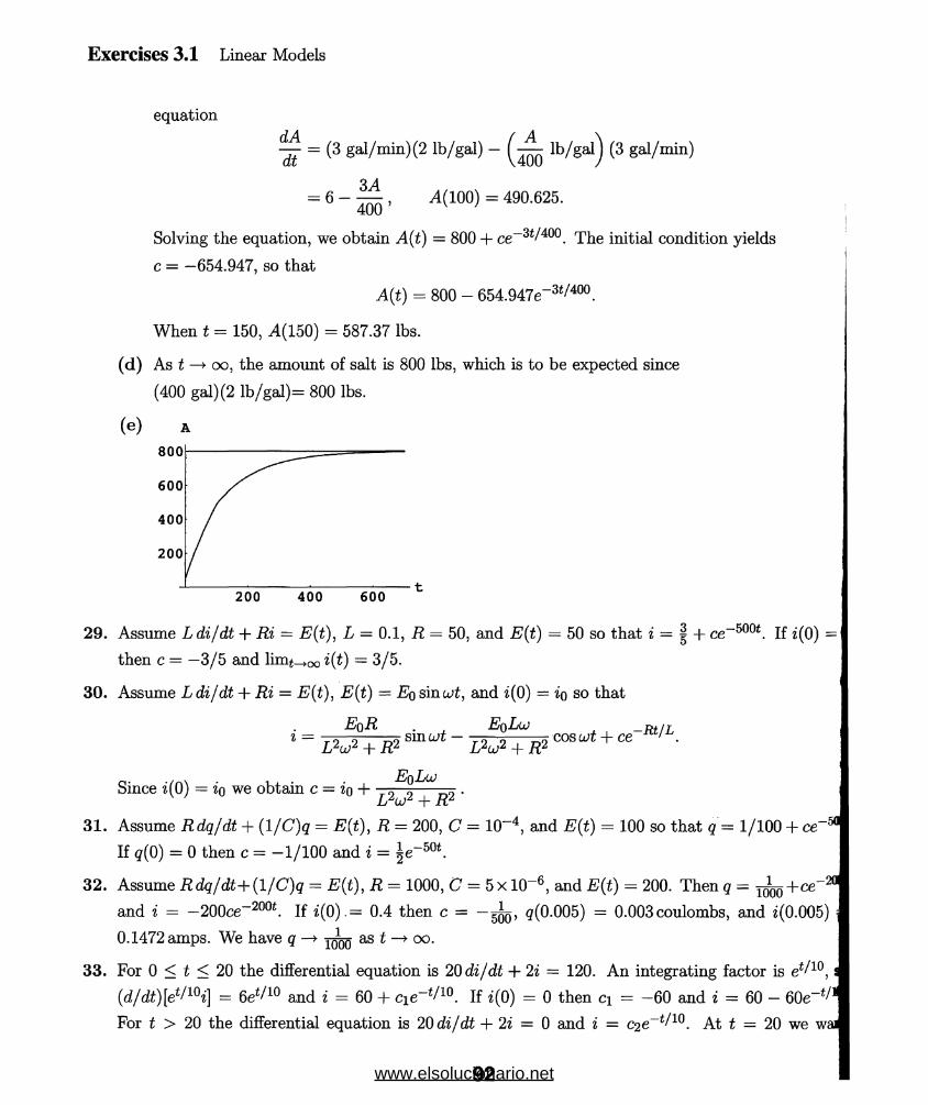
Exercises 3.1 Linear Models
equation
^ = (3 gal/min)(2 lb/gal) - lb/gal) (3 gal/min)
— 6 —3A
400’A(100) = 490.625.
Solving the equation, we obtain A(t) = 800 -I- ce 3*/400. The initial condition yields
c = —654.947, so that
A{t) = 800 - 654.947e_3t/400.
When t = 150, A(150) = 587.37 lbs.
(d) As t —> oo, the amount of salt is 800 lbs, which is to be expected since
(400 gal) (2 lb/gal) = 800 lbs.
(e) a
29. Assume Ldi/dt + Ri = E(t), L = 0.1, R = 50, and E(t) = 50 so that i = | + ce 500t. If i(0) =
then c = —3/5 and lim^oo i(t) = 3/5.
30. Assume L di/dt + Ri = E(t), E(t) = Eq sinu>t, and i(0) = io so that
EoR .... , EqLu ____, , ^-Rt/Li ==
L2u2 + R2sin cot —
L2oj2 + R2cos art + ce
o* */r\\ • i • E0Lu>Since ?(0) = *o we obtain c = %o + To-o-- ^
Lzu)z + Rz
31. Assume Rdq/dt + (1 /C)q — E(t), R = 200, C = 10 4, and E(t) = 100 so that q = 1/100 + ce 50
If <?(0) = 0 then c — —1/100 and i = |e_50t.
32. Assume Rdq/dt+(l/C)q = E{t), R = 1000, C = 5x 10⁻⁶, and E(t) = 200. Then q = i^jj+ce-20
and i = —200ce~200t. If i(0) .= 0.4 then c = — ggg, #(0.005) = 0.003 coulombs, and «(0.005) i
0.1472 amps. We have q 1000 as t oo.
33. For 0 < t < 20 the differential equation is 20 di/dt + 2i — 120. An integrating factor is e*/10, s
(d/(2£)[e*/10i] = 6e*/10 and i = 60 + cie~^10. If i(0) = 0 then c\ = —60 and i = 60 — 60e-^*
For t > 20 the differential equation is 20 di/dt + 2i = 0 and i = C2 e~t/10. At t = 20 we wai
92www.elsolucionario.net

Exercises 3.1 Linear Models
:;t ■ = 60 — 60e 2 so that c2 = 60 (e2 — l) . Thus
J 60 - eOe"^10, 0 < t < 20
*(t) = \60(e2- l)e - ‘/ll», t > 20.
l~. '-i-jjarating variables, we obtain
dg dt
Eq — q/C k\ + k2 t-
I Q-C\r]Eq-±
\ - C
— — In | k\ + *2
(£b ~ q/C)-( k i + h o t ) l '/}'2 2
String q(0) = go we find C2 = (Eq - qo/C)~c /k\/k2 , so
(Ep - q/C)~c (E0 -q0/C)-c
(ki + kit)1 k\ / k 2
C ) \ C ) \k + k2t j
* - § = ( * - § ) (* t k i ) ' /Cb
/ k \ 1/Ck'2
« = £»c + ( « - A»c ) ( ^ J
i a) Prom mdv/dt = mg — kv wc obtain v — mg/k + ce~kt-rn. If v(0) = t’o then c = t’o — mg/k and
the solution of the initial-value problem is
b) As t —> oo the limiting velocity is mg/k.
I c) Prom ds/dt ~ v and s(0) = 0 we obtain
. . m g , m ( mg\ _kt/rr] m ( mg\
fa) Integrating d2s/dt2 = —g we get v(t) = ds/dt = —gt + c. From t’(0) = 300 wc find c = 300,
and we are given g = 32, so the velocity is ?.;(*) = —32* + 300.
■ b) Integrating again and using s(0) = 0 we get s(t) = —16*2 + 300*. The maximum height is
attained when v = 0, that is, at ta = 9.375. The maximum height will be 5(9.375) = 1406.25 ft.
93www.elsolucionario.net
Exercises 3.1 Linear Models
37. When air resistance is proportional to velocity, the model for the velocity is rn dv/dt ~
—mg — kv (using the fact that the positive direction is upward.) Solving the differential equa
tion using separation of variables we obtain v(t) - —mg/k + ce.~kt/m. From t?(0) = 300 wc get
v(t) = + (300 +
Integrating and using s(0) = 0 we find
, (t) _ _ ^ ( + “ (300+ ^ ) ( lSetting k — 0.0025. m = 16/32 = 0.5, and g — 32 we have
s(t) = 1,340.000 - 6,400* - l,340,000e_a0°5t
and
v(t) = -6,400 + 6,700e-0'005*.
The maximum height is attained when v = 0, that is, at ta = 9.162. The maximum height will
s(9.162) = 1363.79 ft, which is less than the maximum height in Problem 36.
38. Assuming that the air resistance is proportional to velocity and the positive direction is downwo..
with .s(0) = 0, the model for the velocity is m dv/dt = my — kv. Using separation of variahl-
to solve this differential equation, we obtain v(t) = mg/k + ce~kt,/'m. Then, using v(0) = 0.
get -u(£) — (mg/k)( 1 — e~kt/m). Letting k — 0.5, m - (125 + 3o)/32 - 5, and g = 32, wc hi-"-
v(t) = 320(1 — Integrating, we find s(t) = 3201 -f 3200e"'°-1i + c\. Solving ,s(0) =
for ci we find ci = —3200. therefore s(t) — 3201 + 3200e“°-1* — 3200. At t = 15, when
parachute opens, i?(15) = 248.598 and s(15) = 2314.02. At this time the value of k change? •
k - 10 and the new initial velocity is vo — 248.598. With the parachute open, the skydiv-. -
velocity is vp(t) - mg/k + C2 (~kL/m, where t is reset to 0 when the parachute opens. Letr:..;
rn — 5. g — 32, and k = 10, this gives vp(t) = 16 + c.2 &~2i. From v(0) - 248.598 wc r.. i1
0 2 — 232.598, so vp(t) = 16+232.598e-2t. Integrating, we get sp(t) = 16£—116.299e_2t+C3. Solv:.
<%(0) = 0 for C'3, we find c» = 116.299. so sp(t) = 16i — 116.299e~2/ +116.299. Twenty seconds "
leaving the plane is five seconds after the parachute opens. The skydivers velocity at this tin:- ’
'^(5) = 16.0106 ft/s and she has fallen a total of $(15) + sp(5) = 2314.02 + 196.294 = 2510.31 "
Her terminal velocity is limt-Kc vp(t) = 16, so she has very nearly reached her terminal vek. '
five seconds after the parachute opens. When the parachute opens, the distance to the groin: -
15,000 — s(lo) = 15,000 — 2.314 = 12,686 ft. Solving sp(t) = 12,686 we get t — 785.6 s = 1
min. Thus, it will take her approximately 13.1 minutes to reach the ground after her parachute . f
opened and a total of (785.6 4- 15)/60 = 13.34 minutes after she exits the plane.
39. (a) The differential equation is first-order and linear. Letting b = k/p, the integrating fact..
94www.elsolucionario.net

Exercises 3.1 Lineax Models
e j 3 b d l / ( b t + r 0) = ( rQ + b t ^ T h e n
- [(?'o + bt)3v] = g(r0 -t- bt)3 and (r0 + bt)3v - J^(r0 + bt)4 + c.
The solution of the differential equation is = (y/46)(?’o + bt) + e(ro + bt)~3. Using v(0) = 0
we find c — —gr^/Ab. so that
= + “ > - •
(b) Integrating dr/ dt — k/p we get r = Atf/p+c. Using r(0) = ryj we have c = ro, so r(t) = /tf/p+ro.
(c) If r = 0.007 ft when t = 10 s. then solving -r(10) = 0.007 for k/p, wTe obtain &/p = —0.0003 and
•r(i) = 0.01 — 0.0003t. Solving r(t) = 0 wc get t = 33.3, so the raindrop will have evaporated
completely at 33.3 seconds.
Separating variables, we obtain d-P/P = k cos t dt, so
In \P\ = k sin t + c and P = ciefcaint.
If P (0) = P0, then ci = P0 and P = PQeks'mt.
(a) From dP/dt = (&i — k})P we obtain P = .p0e^1_fe2 where Po = P(0).
(b) If k-\ > k‘2 then P —» oo as t —> oo. If k\ = % then P = Po for every t. If k\ < k,2 then P —> 0
as t > oo.
(a) The solution of the differential equation is P(t) = c\ekl + h/k. If we let the initial population
of fish be Po then P(0) = Po which implies that
ci = Pq - j± and P(t) = ^P ()- j^ jekt+ y
•b) For Po > h/k all terms in the solution arc positive. In this ease P(t) increases as time t
increases. That is, P(t) —► oc- as i —► oc.
For Pq = h/k the population remains constant for all time t:
For 0 < Po < h/k the coefficient of the exponential function is negative and so the function
decreases as time t increases.
c) Since the function decreases and is concave down, the graph of P(t) crosses the t-axis. That
is, there exists a time T > 0 such that P(T) — 0. Solving
www.elsolucionario.net
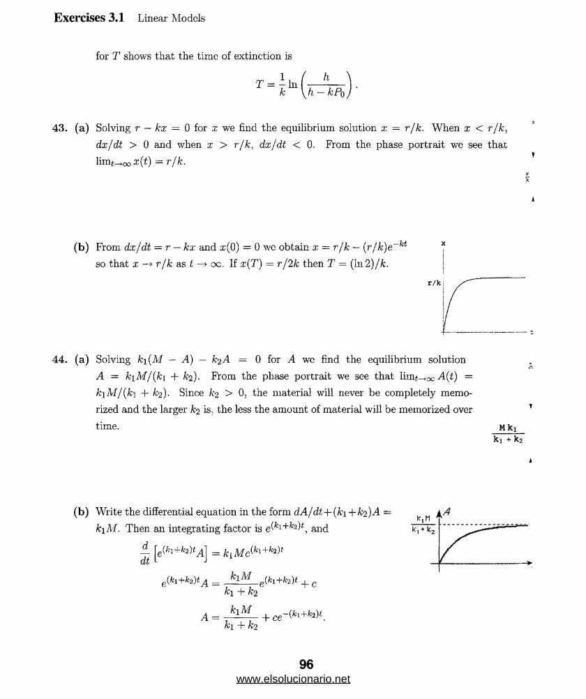
Exercises 3.1 Linear Models
for T shows that the time of extinction is
T = k ln (ft -A:P0) '
43. (a) Solving r — kx = 0 for x we find the equilibrium solution x = r/k. When x < r/k ,
dx/dt > 0 and when x > r/k , dx/dt < 0. From the phase portrait we see that
lim^oo x(t) = r/k.
k
(b) From dx/dt = r — kx and ir(0) = 0 wc obtain x = r/k, — (r/k)e ^ :
so that x —*■ r/k as t —> oc. If x(T) = r/2k then T — (In2)/k.
r/k
44. (a) Solving ki(M — A) — k?A = 0 for A we find the equilibrium solution
A = k\M/(k\ + k^). From the phase portrait we see that A(t) =
k\M/(k\ + k-2 ). Since k-z > 0; the material will never be completely memo
rized and the larger k is; the less the amount of material will be memorized over
time. Mkiki + k2
(b) Write the differential equation in the form dA/dt+(ki+A’2)A =
k\M. Then an integrating factor is e^1+fc2 , and
d = klMe(h+k2)tdt
e(ki+k2)t _ k-lM c(ki+k-2)t _j_ c ki + k2
A =kiM
k\ + k2+ ce -(ki+k2)t
96www.elsolucionario.net
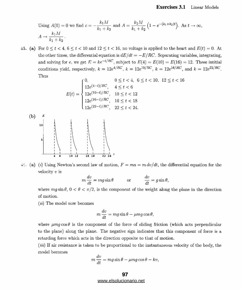
Exercises 3.1 Linear Models
v-r . . /~\ r. i k\M , . A’liU Using .4(0) = 0 wc find c = — ----— and A =
h m
k-i + h
k] + k‘2 k\ + k2(l - e-(h+k-2 )ty As OC,
45. (a) For 0 < t < 4. 6 < t. < 10 and 12 < t < 1C, no voltage is applied to the heart and E(t) = 0. At
the other times, the differential equation is dE/dt = —E/RC. Separating variables, integrating,
and solving for e. we get E = . subject to i?(4) = i?(10) = i?(16) = 12. These intitial
conditions yield, respectively, k = 12e4/'RC, k = \2el<il'RC. k = l2e16‘RC, and k = I2e?2//Rc.
Thus0, 0 < t < 4 , Q < t < 10, 12 < t < 16
12e(i-0/*C 4 < t < 6
12e(io-t)/nc io < t < 12
1 2 e(i6 -i)/RC i 6 < t < igE(t) =
(b)
10
1 L I J4 6 10 12 1 6 1 8 2 2 2 4
4-. (a) (?) Using Newton’s second law of motion, F = ma = mdvjdt, the differential equation for the
velocity v isdv .
m — = mg sm 9 dt
ordv
dt= g sin/9,
where mg sin0, 0 < 9 < tt/2, is the component of the weight along the plane in the direction
of motion.
(ii) The model now becomes
dv .m, — = mg sm 9 — fimq cos a,
dt
where fimg cos 0 is the component of the force of sliding friction (which acts perpendicular
to the plane) along the plane. The negative sign indicates that this component of force is a
retarding force which acts in the direction opposite to that of motion.
(Hi) If air resistance is taken to be proportional to the instantaneous velocity of the body, the
model becomes
77? — = mg sin 9 — fimg cos 9 — kv.
97www.elsolucionario.net

Exercises 3.1 Linear Models
where k is a constant of proportionality.
(b) (i) With m ~ 3 slugs, the differential equation is
, dv 1 dv3 — = (96) • - or — = 16.
dt. 1 2 dt
Integrating the last equation gives v(t) = lQt + c\. Since d(0) = 0, we have c\ — 0 and ^
v(t) = m .
(ii) With m = 3 slugs, the differential equation is
« dv , . 1 \/3 _ . \/3 do3 — = (96) • - - -V • (96) ~ or “77 = 4.
dt v ; 2 4 v ' 2 dt
In this case v(t) = At.
(Hi) When the retarding force due to air resistance is taken into account, the different: ...
equation for velocity v becomes
-.dv 1 y/3 -\/3 1 _dv „ 1 i
3 * = ( 96) ' 2 - T ' (i,6) ' T - 4 (' 01 df = 4
The last differential equation is linear and has solution v(t) = 48 + ci<rf/12. Since t’(0) =
wc find ci = —48, so v(t) = 48 — 48e_i/12.
47. (a) (i) If s(t) is distance measured down the plane from the highest point, then ds/dt — v. In:
grating ds/dt = 16t gives s(t) — 8t2 + Using s(0) = 0 then gives ci = 0. Now the lent.'
L of the plane is L = 50/ sin 30° = 100 ft. The time it takes the box to slide completely dc 3
the plane is the solution of s(t) = 100 or t2 = 25/2, so t « 3.54s.
(ii) Integrating ds/dt = At gives s(t) = 2t2 + C2. Using s(0) = 0 gives c-2 ~ 0, so s(t) = 21? f :
the solution of s(t) = 100 is now t ta 7.07s.
(in) Integrating ds/dt = 48 — 48e-^ 12 and using s(0) = 0 to determine the constant
integration, we obtain s(t) = ASt + 576e_<//12 — 576. With the aid of a CAS we find that
solution of s(t) = 100. or
100 = 481 + 576e_t/12 - 576 or 0 = 48i + 576e~^12 - 676,
is now t « 7.84 s.
(b) The differential equation to dv/dt — mg sin (9 — ftmg cos 6 can be written
m = mg cos (9(tan 6 — fx).LLL
If tan# = ji, dv/dt = 0 and v(0) = 0 implies that v(t) = 0. If tan 0 < // and ?;(0) = 0. : 3
integration implies v(t) = geos0(tan<9 — fi)t < 0 for all time t.
(c) Since tan 23° = 0.4245 and /i = y/Z/A = 0.4330, we see that tan23° < 0.4330. The differs:
equation is dv/dt = 32 cos 23°(tan 23° — y/Z/A) = —0.251493. Integration and the i>
98www.elsolucionario.net
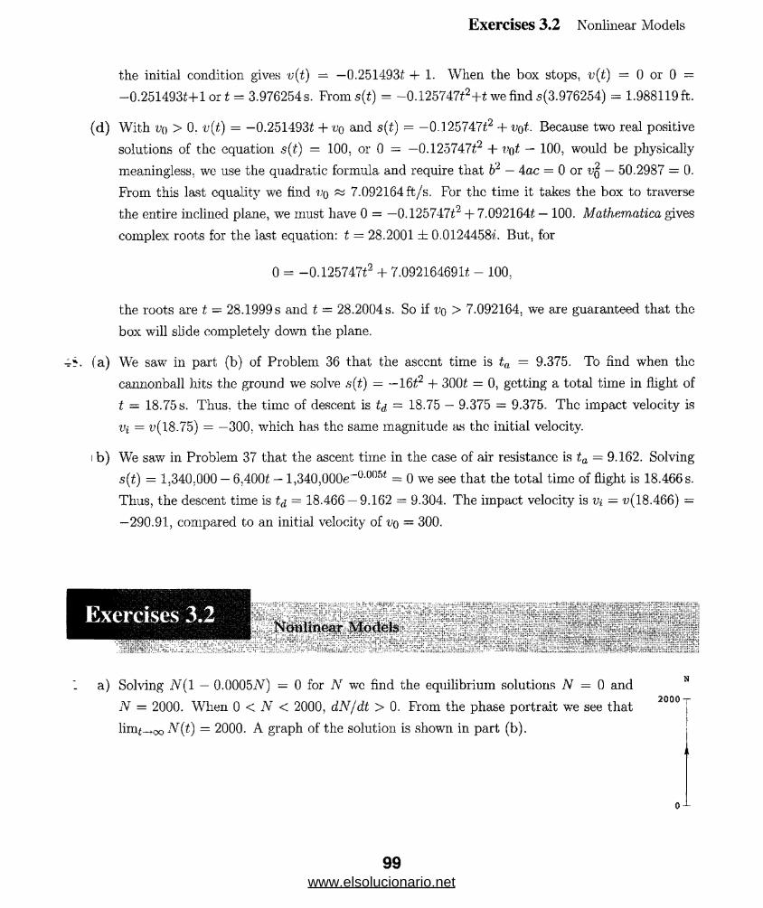
Exercises 3.2 Nonlinear Models
the initial condition gives v(t) = —0.251493t + 1. When the box stops. v(t) = 0 or 0 =
—0.251493i+l or t = 3.976254s. From s(t) = -0.125747t2+i we find s(3.976254) = 1.988119 ft.
( d ) With t*o > 0. v ( t ) = —0.251493i + v q and s(t) = —0.125747f ? + v o t . Because two real positive
solutions of the equation s(t) = 100, or 0 = —0.125747£2 + vot — 100, would be physically
meaningless, we use the quadratic formula, and require that b2 — Aac = 0 or Vq — 50.2987 — 0.
From this last equality we find r'o ~ 7.092164 ft/s. For the time it takes the box to traverse
the entire inclined plane, we must have 0 = —0.125747i2 + 7.092164t — 100. Mathematica gives
complex roots for the last equation: t = 28.2001 ± 0.0124458'i. But, for
0 = —0.125747*2 + 7.09216469li - 100,
the roots are t - 28.1999 s and t — 28.2004 s. So if t’o > 7.092164, we are guaranteed that the
box will slide completely down the plane.
4*. (a) We saw in part (b) of Problem 36 that the asccnt time is ta = 9.375. To find when the
cannonball hits the ground we solve s(t) = —16t2 + 300t = 0, getting a total time in flight of
t = 18.75 s. Thus, the time of descent is = 18.75 — 9.375 = 9.375. The impact velocity is
Vi = i;(18.75) = —300. which has the same magnitude as the initial velocity.
i b) We saw in Problem 37 that the ascent time in the case of air resistance is ta = 9.162. Solving
s(t) = 1,340,000 — 6,400/: — l,340,000e-O'OOM = 0 we see that the total time of flight is 18.466s.
Thus, the descent time is td = 18.466 —9.162 = 9.304. The impact velocity is Vi — u(18.466) —
—290.91, compared to an initial velocity of vq = 300.
.... Ntadtairat.Models... .................. .......; ; !; v? I •
’ ' ‘ "In.;:- TO'
a) Solving jV(l — 0.0005iY) = 0 for N wc find the equilibrium solutions N = 0 and
N = 2000. When 0 < N < 2000, dN/dt > 0. From the phase portrait we see that
lim*—oo N(t) = 2000. A graph of the solution is shown in part (b).
o-1
99www.elsolucionario.net
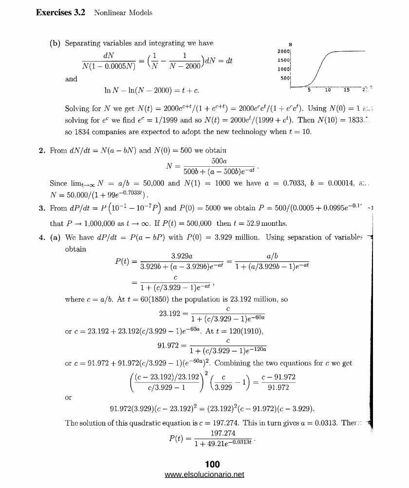
Exercises 3.2 Nonlinear Models
(b) Separating variables and integrating we have
dN (1 1 \ T _
(/\T ~~ N - 2000) 1' ~ ( tN{1 - 0.0005A') \N N - 2000
and
In Ar- ln(iV - 2000) = t + c.
Solving for N we get N(t) = 2000cc+t/ ( l + ec+f) = 2000creV(l -f e'V). Using A7(0) = 1 e.:
solving for ec we find ett = 1/1999 and so N(t) = 2000e'/(1999 + eL). Then JV(10) = 1833.'
so 1834 companies are expected to adopt the new technology when t = 10.
2. From dN/dt = N(a — bN) and Ar(0) — 500 we obtain
... 500aA' =
5006 + (a — 5006) e at
Since l i m ^ Ar = a/b = 50,000 and Ar(l) - 1000 we have a = 0.7033, b = 0.00014, a:..
N = 50.000/(1 + 99e-°-7033<) .
3. From dP/dt = P (l0 _1 - 10_7P) and P(0) = 5000 we obtain P = 500/(0.0005 + 0.0995e-°JJ '3
that P —> 1.000,000 as I —>■ oo. If P(t) = 500:000 then t — 52.9 months.
4. (a) We have dP/dt = P(a — bP) with P(0) = 3.929 million. Using separation of variable?
obtain3.929a a/b
p(t) =3.9296 + (a - 3.929f>)e-“' 1 + (a/3.929b - l)e~“
c
1 + (c/3.929 - 1)e~at ’
where c = a/b. At t = 60(1850) the population is 23.192 million, so
93 loo ■_________ -_________1 + (c/3.929 - l)e-60°
or c = 23.192 + 23.192(c/3.929 - l)e“60a. At t = 120(1910),
91.972 =1 + (c/3.929 - l)e-120a
or c = 91.972 + 91.972(c/3.929 — l)(('_60a)2. Combining the two equations for c we get
(c - 23.192)/23.192>\2 ( c \ _ c - 91.972
V c/3.929- 1 j V 3.929 ) 91.972
or\2 _ /oo -irv~>\291.972(3.929)(c - 23.192)2 = (23.192)2(c - 91.972)(e - 3.929).
[uation i
p(t) =
The solution of this quadratic equation is c = 197.274. This in turn gives a = 0.0313. Then:
197.274
1 + 49.21e-°-0313t '
100www.elsolucionario.net
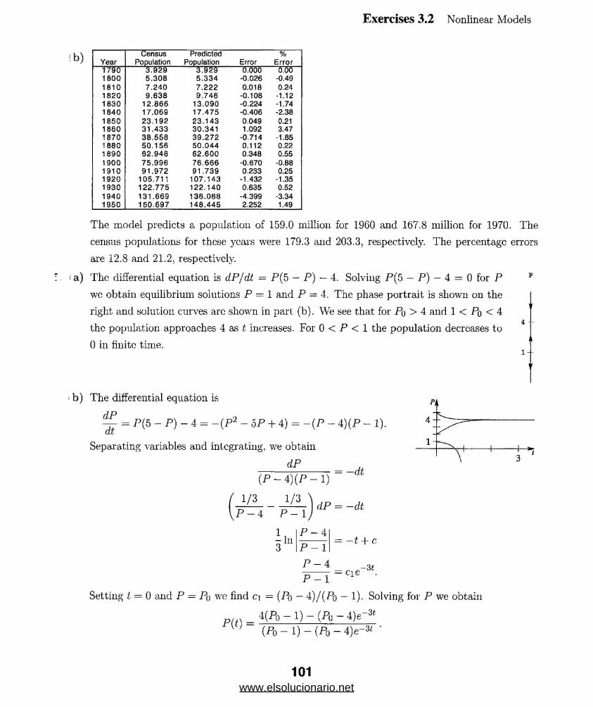
Exercises 3.2 Nonlinear Models
•b) YearCensus
PopulationPredicted
Population Error%
Error1790 3.929 3,929 0.000 6.001800 5,308 5.334 -0.026 -0.491810 7.240 7.222 0.018 0.241820 9.638 9.746 -0.108 -1.121830 12.866 13.090 -0.224 -1.741840 17.069 17.475 -0.406 -2.381850 23.192 23.143 0.049 0.211860 31.433 30.341 1.092 3.471870 38,558 39.272 -0.714 -1.851880 50.156 50.044 0.112 0.221890 62.948 62.600 0.348 0.551900 75.996 76.666 -0.670 -0.881910 91.972 91.739 0,233 0.251920 105.711 107.143 -1.432 -1.351930 122.775 122.140 0,635 0.521940 131,669 136.068 -4.399 -3.341950 150.697 148.445 2.252 1.49
The model predicts a population of 159.0 million for 1960 and 167.8 million for 1970. The
census populations for these years were 179.3 and 203.3, respectively. The percentage errors
are 12.8 and 21.2. respectively.
: . i a) The differential equation is dP/dt = P (5 — P) — 4. Solving P(5 — P) — 4 = 0 for P p
we obtain equilibrium solutions P = 1 and P = 4. The phase portrait is shown on the
right and solution curves arc shown in pari: (b). We see that for Pq > 4 and 1 < Po < 44 * -
the population approaches 4 as £ increases. For 0 < P < 1 the population decreases to
0 in finite time. i —v
b) The differential equation is
dP
dt= P(5 - P) - 4 = - (P 2 - 5P + 4) = - (P - 4)(P - 1).
Separating variables and integrating, we obtain
dP
(P - 4 )(P - 1 )
1/3 1/3
= -d t
P — 4 P - 1
1 P — 4
3 hl
dP = —dt
P - 1
P — 4
P - l
= -t + c
- c\e -31
Setting I = 0 and P = Po we find ci = (Po — 4)/(Po — 1). Solving for P we obtain
4(P0 - l ) - ( P 0 -4)e-3*P(t) =
(P0 - l ) - ( P 0 -4)e-3/' •
101www.elsolucionario.net

Exercises 3.2 Nonlinear Models
(c) To find when the population becomes extinct in the case 0 < Pq < 1 we set P = 0 in
P - 4 = By-4 ,t
P - 1 F o - 1 '
from part (a) and solve for t. This gives the time of extinction
3 P0 -4
6 . Solving P (5 — P) — ^ = 0 for P we obtain the equilibrium solution P = | . For P ^ | . dP/dt < 0.
Thus, if Pq < | , the population becomes extinct (otherwise there would be another equilibrium
solution.) Using separation of variables to solve the initial-value problem, wc get
P(t) = [4P0 + (lOPo ~ 25)t]/[4 + (4Pa - 10)t].
To find when the population becomes extinct for Pq < % we solve P(t) = 0 for t. We see that the
time of extinction is t = 4Po/5(5 — 2Po).
7. Solving P (5 — P) — 7 = 0 for P we obtain complcx roots, so there are no equilibrium solutions.
Since dP/dt < 0 for all values of P, the population becomes extinct for any initial condition. Usku
separation of variables to solve the initial-value problem, we get
_! (2Pq — 5'tan
V3
Solving P(t) = 0 for t we see that the time of extinction is
t — ^(\/3tan 1 (5/^3) + V3 tan 1[(2Po — 5)/\/3]).
8. (a) The differential equation is dP/dt = P( 1 — InP), which has the equi
librium solution P = e. When Po > e, dP/dt < 0, and when Pq < e,
dP/dt > 0.
(b) The differential equation is dP/dt = P( 1 + InP), which has the equilib
rium solution P = 1/e. When Po > 1/e. dP/dt > 0, and when Po < 1/e,
dP/dt < 0.
(c) From dPjdt = P(a — bInP) we obtain —(1/6)In |a — 61nP| = t + c\ so that P = ea/t)e ce
If P (0) = Pq then c = (a/b) — In Po-
102www.elsolucionario.net
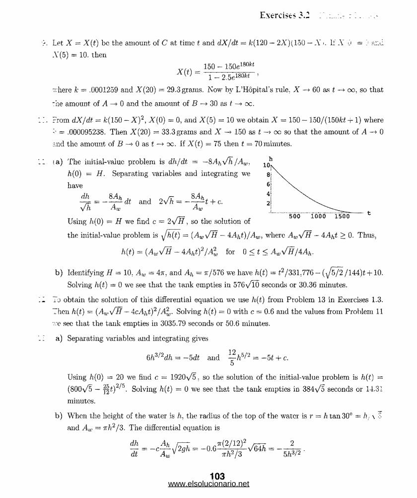
Exercises 3.2
Let X = X(i) be the amount of C at time t and dX/dt = k( 120 — 2A')(150 — X >. If A" 0 = j a:.c
A(5) = 10. then
_ 150 — 150e18OW
l-2 .5e180** ’
■."here k = .0001259 and A (20) = 29.3 grams. Now by L;H6pital's rule. X —► 60 as t —> oo, so that
the amount of A —> 0 and the amount of B —► 30 as t —> oc.
From dXjdt = A:(150 — A’)2, A"(0) = 0, and X(5) = 10 we obtain X = 150 — 150/(150H + 1) where
= .000095238. Then X (20) = 33.3 grains and A' —»• 150 as t —* oo so that the amount of A —» 0
and the amount of B —> 0 as t —► oc. If X (t) = 75 then t = 70 minutes.
i.a) The initial-value. problem is dh/dt = —&AhVh/Aw< 10
h.(0) = H. Separating variables and integrating we
have
= aad 2 Vh = - ^ ~ t + c.y/h Aw A.w
Using h(0) = H we find c = 2y/H , so the solution of
the initial-value problem is \Jh(t) = (Aw\fH — 4Aht)JAw, where Awy/H — 4,4/,t > 0. Thus.
ft(*) = (Atov/ff - A A htf!/^ for 0 < t < A.wy/~H/4Ah.
b) Identifying H = 10. Aw = 4tt, and Ah = tt/576 we have h(t) = £2/331.776 — (y 5/2 /144)t +10.
Solving ft,(i) - 0 we see that the tank empties in 576\/l0 seconds or 30.36 minutes.
To obtain the solution of this differential equation we use h(t) from Problem 13 in Exercises 1.3.
Then h(t) = (Aw'/H — AcA^t)2 jA2W. Solving h(t) = 0 with c = 0.6 and the values from Problem 11
■ve see that the tank empties in 3035.79 seconds or 50.6 minutes.
a) Separating variables and integrating gives
6 h?^dh = —5 dt and ~ h b/2 = —51 + c.5
Using h(0) = 20 we find c = 1920\/5. so the solution of the initial-value problem is h(t) =
(800\/5 — j§i)2/J. Solving h(t) = 0 we see that the tank empties in 384\/5 seconds or 14.31
minutes.
b) When the height of the water is h, the radius of the top of the water is r = h tan 30° = h , \ 3
and Aw = irh2/Z. The differential equation is
^ = _o.6^ ( ^ | ! v 6S = — L .dt Aw v y trh2/S 5ft3/2
103www.elsolucionario.net

Exercises 3.2 Nonlinear Models
Separating variables and integrating gives
5h:i' 2dh — —2 dt and 2/?5/2 = —21 + c.
Using h(0) 9 we find c, = 486. so the solution of the initial-value problem is h(t) = (243—£)2'"
Solving h(t) = 0 we see that the tank empties in 243 seconds or 4.05 minutes.
14. When the height of the water is h, the radius of the top of the water is |(20 — h) ar.
Aw = 4tt(20 — h)'2/25. The differential equation is
dh Ah p y j tt(2/ 12)2 ^ 5 Vh.- = - c j - ^ g h = - 0 - \ w{20_ h)2/25^ = - g poTftjJ •
Separating variables and integrating we have
(20 — ft)2 5 4nA /r 80,,,., 2dh = --dt and 800VTi — ^~h3/2 + -ft0/2 = — -t + c.
yfh 6 3 5 6
Using /).(0) = 20 we find c = 2560\/5/3, so an implicit solution of the initial-value problem is
3 b 6 3
To find the time it takes the tank to empty wc set h = 0 and solve for t. The tank empties
1024\/5 seconds or 38.16 minutes. Thus, the tank empties more slowly when the base of the cc:.
is on the bottom.
15. (a) After separating variables we obtain
m dv
mg — kv2
1 dv
= dt
— dtg 1 - (y/kv/y/mg)2
y/mg yf k/mg dv _
Vk g 1 - (Vkv/y/mg )2
!m , _i y/kv 1 —- tanh _ = t + c. kg s/mg
taah-’ ^ = M t + C i .Jm g V rn
Thus the velocity at time t is
Setting t = 0 and v = t’o wc find c\ = tanh“”1 (yfk. ?;q/ y / r n g ).
104www.elsolucionario.net

Exercises 3.2 Nonlinear Models
b) Since tanh t —> 1 as t —* oo, we have v —► yjmgfk as t —> oc.
c) Integrating the expression for v(t) in part (a) we obtain an integral of the form f du/u:
[kg \ m ,cosh | y' — t + ci
rn+ C2.
Setting i = 0 and s = 0 we find c<i = —(m/k) ln(coshci), where ci is given in part (a),
rhe differential equation is m, dv/dt. = —mg — kv2. Separating variables and integrating, we have
dv dt
mg + hiP- m
1 _i f Vkv\ 1tan - = -- 1 + c
■\/mgk \y/mg J m
_i ( Vkv\ jgk tan ,__ = — \ — t + ci\y/rng) V m
Sotting t!(0) = 300, m = \ , g = 32, and k — 0.0003, we find v(t) = 230.94 tan(ci — 0.138564£)
'lid Ci = 0.914743. Integrating
,;(*) = 230.94 tan(0.914743 - 0.138564*)
v:e get
s{t) = 1666.67In | cos(0.914743 - 0.138564*) | + c2.
"."sing ,s(0) = 0 we find c-i = 823.843. Solving v(t) = 0 we see that the maximum height is attained
-•hen t = 6.60159. The maximum height is s(6.60159) = 823.843 ft.
I", t a) Let p be the weight density of the water and V the volume of the object. Archimedes’ principle
states that the upward buoyant force has magnitude equal to the weight of the water displaced.
Taking the positive direction to be down, the differential equation is
dv , 2m — = mg — kv — pv.
dt
( b) Using separation of variables we have
m dv
(mg — pV) — kv2
m Vk dv
\/k (s/mg — pV )2 — (Vkv)2
= dt
= dt
TO 1 i- l ySk'v _±
y/k V m 9 - pV tan 1 V ’ g - pV + c
105www.elsolucionario.net
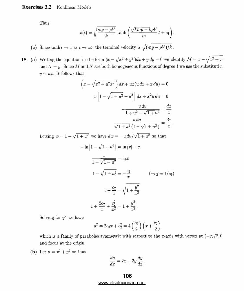
Exercises 3.2 Nonlinear Models
Thus
. . imq - pV , , (\Jknig — kpV .
v(f) - \! ~ ^ r — tanh I -— "— * + ci I •TO
(c) Since tanh t —> 1 as t —► oo, the terminal velocity is y' (rng — pV )fk .
18. (a) Writing the equation ill the form (x — yjx2 + y2 )dx + y dy = 0 we identify M = x — y/x2 + , -
and N = y. Since M and N are both homogeneous functions of degree 1 we use the substitutk
y = ux. It follows that
{x- — \jx2 — u2x2 dx + ux(udx + xdu) = 0
x 1 — \j\ + ifi + u2 dx + x2u du — 0
u du dx
1 - f U 2 — \ / l + U2 X
■udu _ dx
‘ xV l + u2 (l — v i + t? )
Letting w = 1 — v T T t? we have dw = —udu/V l + u2 so that
— In 1 — \J 1 + u2 — In jz| + c
1Cjx
1 — V l 4- u2
1 - y/l +u2 = (-C2 - l/'ci)
1+? = V1+S2 C‘2 , A y
Solving for y2 we have
1 H-- 11 H— | — 1 H— 2 •X X* x z
y2 = 2c2x + 4 = 4 x +C2
which is a family of parabolas symmetric with respect to the x-axis with vertex at (—1‘2/2,C
and focus at the origin.
(b) Let u — x2 + y2 so that
du n n dy
T x ~ 2x + 2ydi-
106www.elsolucionario.net
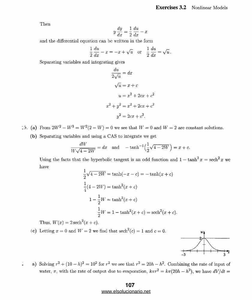
Exercises 3.2 Nonlinear Models
Thendy 1 du
and the differential equation can be mitten in the form
1 du 1 da_ _ _ I = _X.+V^ or - Tx = ^ .
Separating variables and integrating gives
du .——7= = dx2 y/u
y/u = X + C
u = x2 + 2 cx + c,2
x2 + y2 = x2 + 2cx -j- c2
y2 = 2cx + c2.
.9. (a) From 2W 2 - W 3 = W 2{2 - W) = 0 we see that W = 0 and W = 2 are constant solutions.
( b ) Separating variables and using a CAS to integrate we get
-- = dx and — tanh-1 f \/ 4 — 2W ) = x + c.WV4 - 2 W y2 t
Using the facts that the hyperbolic tangent is an odd function and 1 — tanh2 x = sech2 x wc
have
—\/4 — 2W — tanh(—x — c) = — tanh(x + c)z
i(4 - 211’) = tanh2 (a: + c)
1 — \-W = tanh2 (a; + c)z
^ 11' = 1 — tanh2 (a: + c) = sech2 (a; + c).
Thus. TTr(rc) = 2 sech2 (re + c).
(c) Letting x = 0 and W = 2 we find that sech2(c) = 1 and c = 0.
a) Solving r2 + (10 — h)2 = 102 for r2 we see that r2 = 20/i — ti2. Combining the rate of input of
water, ir, with the rate of output due to evaporation.; hnr2 = kir(20h — /i2), wc have dV/dt =
107www.elsolucionario.net
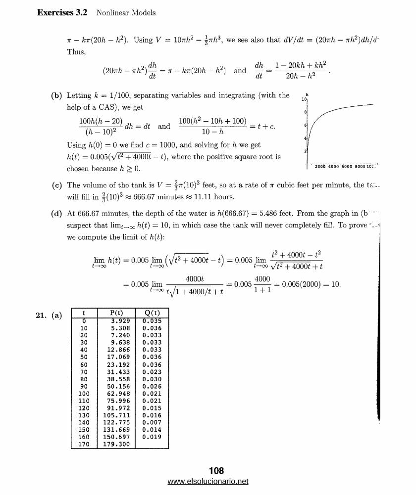
Exercises 3.2 Nonlinear Models
7T — kir(20h — h2). Using V — IOtt/i2 — vh3, we see also that dV/dt = (20tt/x — ixh?')dhjd:
Thus.
/ , , ‘>\dh , , , 9a . rf/i l — 2()kh + kh2(207r/i — tr/i )— = 7T — &7r(20/?- — /r) and — = --——-- --- .v 1 dt v dt 20h - h
(b) Letting k — 1/100, separating variables and integrating (with the
help of a CAS), we get
100h(h — 20) „ , , 100(fr2 - 10ft + 100)
(A - 10)» d h = d t “ d 10-fc------ = f + C'Using h(0) = 0 we find c = 1000, and solving for h. we get
h(t) = 0.005(\/t2 + 4000i — t), where the positive square root is
chosen because h > 0.
(c) The volume of the tank is V = |tt(10)3 feet, so at a rate of nr cubic feet per minute, the ta:
will fill in §(10)3 « 666.67 minutes ~ 11.11 hours.
(d) At 666.67 minutes; the depth of the water is ft(666.67) = 5.486 feet. From the graph in (b '
suspect that linv_>cc h(t) — 10, in which case the tank will never completely fill. To prove '1
we compute the limit of h(t):
t2 + 4000t - t2lim h(t) = 0.005 lim ( J t 2 + 4000t - 1) = 0.005 limt— >00 f—>OC V / t— >OCt-400
n V 4 0 0 0 t= 0.005 lim — , --^ ° ° tyj 1 + 4000/t + 1
t-*00 Vt2 + 4000t + 1
O.OOS = 0.005(2000) = 10.
21. (a) t P(t) Q(t)0 3.929 0.03510 5.308 0.03620 7.240 0.03330 9.638 0.03340 12.866 0.03350 17.069 0.036
60 23.192 0.03670 31.433 0.023SO 38.558 0.03090 50.156 0.026100 62.948 0.021110 75.996 0.021120 91.972 0.015130 105.711 0.016140 122.775 0.007150 131.669 0.014160 150.697 0.019170 179.300
108www.elsolucionario.net

Exercises 3.2 Nonlinear Models
b) The regression line is Q = 0.0348391 — 0.000168222P.
Q
0.035*
0.03!
20 40 60 80 100 120 140
c) The solution of the logistic equation is given in equation (5) in the text. Identifying a ==
0.0348391 and b = 0.000168222 we have
aPQ
bPo -f (a — bP(\)e~at'
d) With P0 = 3.929 the solution becomes
P(f) =0.136883
0.000660944 + 0.0341781fi-° o34839u '
e)
f ) We identify t = 180 with 1970, t = 190 with 1980, and t, ~ 200 with 1990. The model predicts
P(180) = 188.661, P(190) = 193.735, and P(200) = 197.485. The actual population figures
for these years are 203.303, 226.542, and 248.765 millions. As t —► oc, P(t) —> a/b = 207.102.
a) Using a CAS to solve P (1 — P) + 0.3e_jP = 0 for P we see that P = 1.09216 is an equilibrium
solution.
b) Since /(P ) > 0 for 0 < P < 1.09216, the solution P(t) of f
dP/dt = P (1 - P) + Q.3e~F, P (0) = P0,
is increasing for Po < 1.09216. Since f(P ) < 0 for P > 1.09216. the
solution P(t) is decreasing for Po > 1.09216. Thus P = 1.09216 is
a.n attractor.
109
.‘5 2 2T5 3 p
www.elsolucionario.net
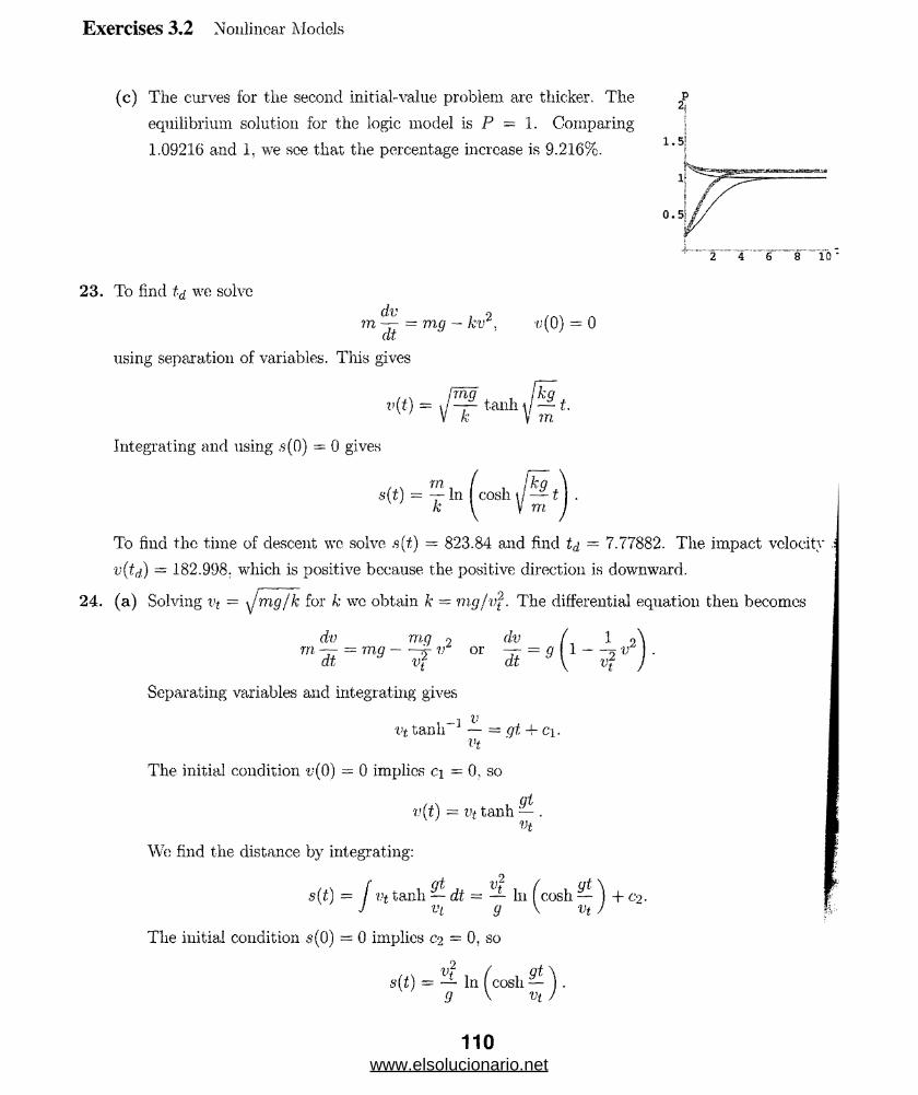
Exercises 3.2 Nonlinear Models
(c) The curves for the second initial-value problem are thicker. The
equilibrium solution for the logic model is P = 1. Comparing
1.09216 and 1, we see that the percentage increase is 9.216%.
23. To find id we solve
dv 2m — = ni,q — kv .
dt J
using separation of variables. This gives
*(0) = 0
kg
Integrating and using ,s-(0) = 0 gives
s(t) = y In ( cosh \j — t j .____k \ V m
To find the time of descent we solve s(t) = 823.84 and find t(i = 7.77882. The impact velocity
v(td) = 182.998; which is positive because the positive direction is downward.
24. (a) Solving vt = yjmg/k for k we obtain k = rngjvj. The differential equation then becomes
dv mg . 2m — = mg - - ^
dt vf
Separating variables and integrating gives
dv ( 1 2\
dt
vt tanh-1 — = at + c\.vt
The initial condition v(0) = 0 implies c\ = 0, so
v(t) = Vt tanh — .vt
We find the distance by integrating:
s(t) = j vt tanh — dt = — In ( cosh — \ -f 0 2 ■ J vt. 9 V vt J
The initial condition s(0) = 0 implies C2 = 0, so
S(t) = i In (cosh9 V vt )
110www.elsolucionario.net
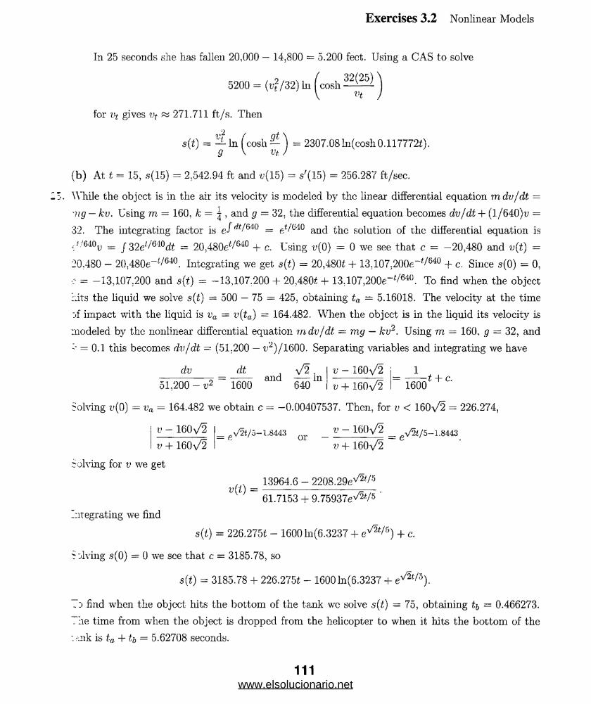
Exercises 3.2 Nonlinear Models
In 25 seconds she has fallen 20,000 — 14,800 = 5.200 feet. Using a CAS to solve
5200 = (v2 /32) In |cosh ^
for vt gives vt ~ 271.711 ft/s. Then
s(t) = -^-ln ^cosh — ^ = 2307.08 ln(cosh 0.117772*).
(b) At t - 15, s(15) = 2.542.94 ft and t/(15) = /(W ) = 256.287 ft/sec.
While the object is in the air its velocity is modeled by the linear differential equation mdv/dt =
'ng — kv. Using m - 160, k = \ , and g ~ 32, the differential equation becomes dv/dt + (l/640)v =
32. The integrating factor is eJ d t / 6 4 0 = e*/G40 an(j ^1C soiution of the differential equation is
i t/Q4av = J 32el/tii0dt = 20,480e</640 + c. Using t;(0) = 0 we see that c = —20,480 and v(t) =
20,480 - 20,480e_t/640. Integrating we get s(t) = 20,4801 + 13,107.200e~t/64° + c. Since s(0) = 0,
;■ = -13,107,200 and s(t.) = -13,107,200 + 20,480* + 13,107,200e"</640. To find when the object
hits the liquid we solve s(t) = 500 — 75 = 425, obtaining ta = 5.16018. The velocity at the time
jf impact with the liquid is va = v(ta) = 164.482. When the object is in the liquid its velocity is
modeled by the nonlinear differential equation mdv/dt ~ mg — kv2. Using m = 160, g = 32, and
= 0.1 this becomes dv/dt - (51.200 — i ’2)/1600. Separating variables and integrating we have
v - 160\/2 1dv dt \ / 2
51,200 — v2 1600 aU 640 Q v) + 160\/2 1600t + C.
Solving v(0) = t'a = 164.482 we obtain c = —0.00407537. Then, for v < 160\/2 = 226.274,
v 160\/2
v + 160\/2
Solving for v we get
_ ev ’2t/5—1.8443 or _ v ~ 160\/2 _ eV2f/5_i.8443
V + 160V2
, , 13964.6 - 2208.29e^/3 v(t) =
61.7153 + 9.75937e^/5 '
Integrating we find
s(i) = 226.2751 - 16001n(6.3237 + e ^ 5) + c.
S jiving ,s(0) = 0 we see that c = 3185.78, so
s(*) = 3185.78 + 226.275* - 16001n(6.3237 + e^2tr°).
Tj find when the object hits the bottom of the tank wc solve s(t) = 75, obtaining = 0.466273.
The time from when the object is dropped from the helicopter to when it hits the bottom of the
*.::.nk is ta +tb = 5.62708 seconds.
111www.elsolucionario.net
Exercises 3.2 Nonlinear Models
26. The velocity vector of the swimmer is
v = Vs + v.r = (—v8 cos$, —vs sin0) + (0. vr) = (-vs cos 0. -va sin^ 4- vr) = ~jfj
Equating components gives
so
Thus.
dx . . dy . .— = — vs cos 0 and — = —vv sm 0 + vr dt " dt
dx x dy y— = - v a r~.------ — a n d “ 77 “ ~ V s r ---------= + tv -
JX 2 + IJ2 dt /,};2 y2
dy _ dy/dt _ -vHy -i- vryjx2 + y2 _ vsy - vryjx2 + y2 dx dx/dt —vsx V/fX
27. (a) With k = vr/vs,
dy _ y ~ kyjx2 + y2
dx x
is a first-order homogeneous differential equation (see Section 2.5). Substituting y = ux int:
the differential equation gives
du 7 r r du , r I■u + x— = u — kv 1 + vr or — = —k\j 1 + uz.
dx dx
Separating variables and integrating we obtain
j = — J k dx or In + \j 1 + u2 j = — k In x + In c.
This implies
y ( v / x 2 + y 2 ' f =In xk + yj 1 + u2 ^ = In c or xk I — +
X
The condition y( 1) = 0 gives c = 1 and so y + \jx2 + y2 — x^~k. Solving for y gives
J/(*) = \ {*l~k ~ a;1+fc) •
(b) If k = 1, then vs = vr and y = ^(1 — x2). Since y(0) = 5, the swimmer lands on the we*'
beach at (0. ^). That is. I mile north of (0,0).
If k > 1. then vr > vs and 1 — k < 0. This means lim;t._>0+ y(x) becomes infinite, sin-.-
liinx_>0+ xl~lc becomcs infinite. The swimmer never makes it to the west beach and is swe:'
northward with the current.
If 0 < k < I, then vs > vr and 1 — k > 0. The value of y(x) at x = 0 is y(0) = 0. The swimm-
has made it to the point (0,0).
112www.elsolucionario.net
Exercises 3.2 Nonlinear Models
28. The velocity vcctor of the swimmer is
Equating components gives
so
29. The differential equation
dx , dy— = -va and -7- = vr dt dt
dy _ dy/dt _ vr __ vr
dx dx/dt —Vs va'
dy 30 a.-(1 — x)
dx 2
separates into dy — lo{—x + x2)dx. Integration gives y(x) = — •y.T2 + ox3 + c. The condition
7/(1) = 0 gives c = | and so y(x) = ^(—l-5x2 + l().r3 + 5). Since y(0) = |. the swimmer has to walk
2.5 miles back down the west beach to reach (0,0).
30. This problem has a great many components, so we will consider the case in which air resistance is
assumed to be proportional to the velocity. By Problem 35 in Section 3.1 the differential equation
is
and the solution is
dvm—- = mg — kv,
dt
If we take the initial velocity to be 0, then the velocity at time t is
v(t) = ^n.- rC
The mass of the raindrop is about m = 62 x 0.000000155/32 « 0.0000003 and g = 32, so the
volocitv at time t is0.0000096 _ 0.0000096 333333*
k k
If we let k = 0.0000007, then v(100) ~ 13.7 ft/s. In this case 100 is the time in seconds. Since
7 mph m 10.3 ft/s, the assertion that the average velocity is 7 mph is not unreasonable. Of course,
this assumes that the air resistance is proportional to the velocity, and, more importantly, that
the constant of proportionality is 0.0000007. The assumption about the constant is particularly
suspect.
:■!. (a) Letting c = 0.6. A/,. = tt(^ Aw = tt • l 2 = it, and g = 32. the differential equation
in Problo 12 becomes dh/dt. = —0.00003255\/ft • Separating variables and integrating, we get
2y/h = -0.00003255* + c, so h = (ct - 0.00001628t)2. Setting h(0) = 2, we find c = y/2, so
h(t) = (V ^ - 0.00001628i)2, where h is measured in feet and t in seconds.
113www.elsolucionario.net
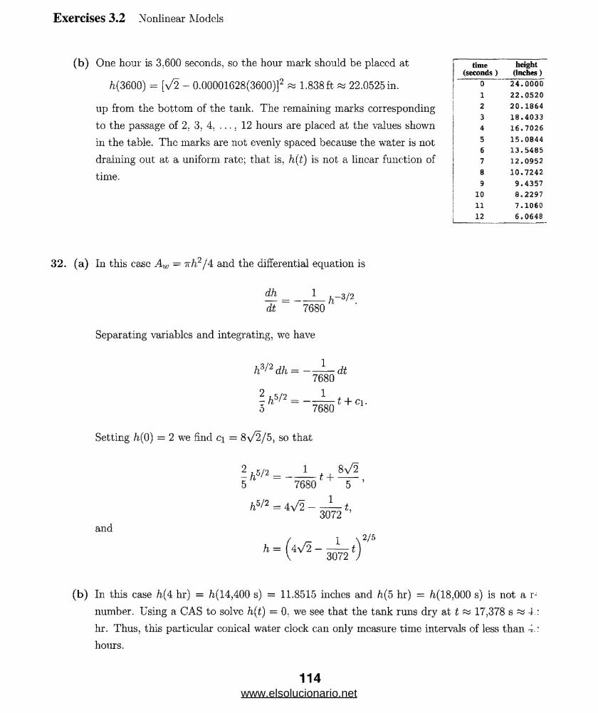
Exercises 3.2 Nonlinear Models
(b) One hour is 3.600 seconds, so the hour mark should be placed at
/i(3600) = [V2 - 0.00001628(3600)]2 « 1.838 ft- « 22.0525 in.
up from the bottom of the tank. The remaining marks corresponding
to the passage of 2. 3, 4. ... . 12 hours are placed at the values shown
in the table. The marks are not evenly spaced because the water is not
draining out at a uniform rate; that is, h(t) is not a linear function of
time.
time (seconds ) height (inches)0 24* 00001 22«05202 20 .1 86 43 18 .4 03 34 16 .7 02 65 15 .084 46 13 .5 4857 12 .09528 10 ,724 29 9 . 4357
10 8 . 229711 7 .106012 6 .0648
32. (a) In this case Aw = tt/i2/4 and the differential equation is
dh 1
dt 7680
Separating variables and integrating, we have
h-V2.
h3/2dh = - — rdt7680
^5 /2 _____— t + ci0 7680 +Cl'
Setting h(0) = 2 we find c\ = 8\/2/5, so that
5 7680 5
/i5/2 = 4 y/23072
t,
and
(b) In this case h(4 hr) = /i(14,400 s) = 11.8515 inches and h(5 hr) = ft(18,000 s) is not a r-
number. Using a CAS to solve h(t) = 0. we see that the tank runs dry at t ~ 17,378 s ~ 4
hr. Thus, this particular conical water clock can only measure time intervals of less than 4.
hours.
114www.elsolucionario.net
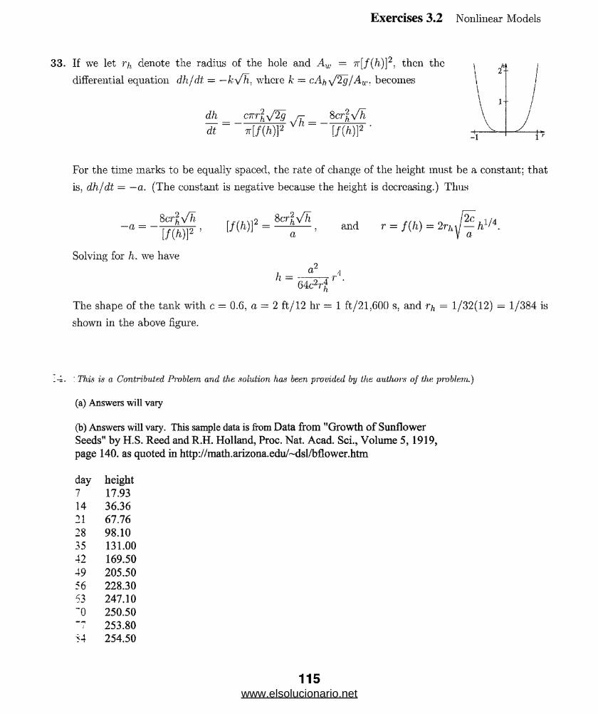
Exercises 3.2 Nonlinear Models
33. If we let r/( denote the radius of the hole and Aw — tt[/(/i)]2, then the
differential equation dh/dt — —k /h.. where k — cA \/2gjAv,. becomes
d h C n r j. v/2g r- 8cr?\fh.
^ = - W W vh = - W W -1
For the time marks to be equally spaced, the rate of change of the height must be a constant; that
is. d h / d t = — a . (The constant is negative because the height is dccrcasing.) Thus
_ Scr^vTi
~a = ~ J f W ’
Solving for h. we have
[ m f = 8craand r = f ( h ) = 2r/,, y ^ h 1^4 .
h =a
Uc2rft
The shape of the tank with c = 0.6, a = 2 ft/12 hr = 1 ft/21,600 s, and >7,. = 1/32(12) — 1/384 is
shown in the above figure.
:-k. : This is a Contributed, Problem and the solution has been provided by the authors of the problem.)
(a) Answers will vary
(b) Answers will vary. This sample data is from Data from "Growth of Sunflower
Seeds" by H.S. Reed and R.H. Holland, Proc. Nat. Acad. ScL, Volume 5,1919,
page 140. as quoted in http://math.arizona.edu/~dsl/bflower.htm
day height7 17.9314 36.3621 67.76
28 98.10
35 131.0042 169.50
49 205.5056 228.3062 247.10"0 250.50
253.80-?4 254.50
115www.elsolucionario.net
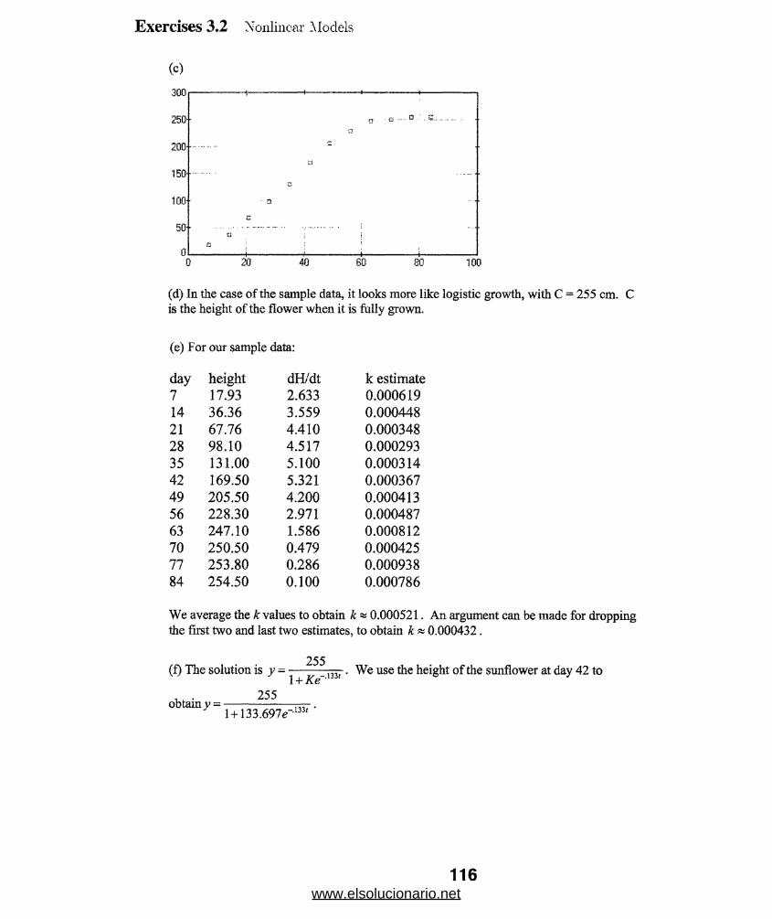
Exercises 3.2 Nonlinear Models
(d) In the case of the sample data, it looks more like logistic growth, with C = 255 cm. C is the height of the flower when it is fully grown.
(e) For our sample data:
day height dH/dt k estimate7 17.93 2.633 0.00061914 36.36 3.559 0.00044821 67.76 4.410 0.00034828 98.10 4.517 0.00029335 131.00 5.100 0.00031442 169.50 5.321 0.00036749 205.50 4.200 0.00041356 228.30 2.971 0.00048763 247.10 1.586 0.00081270 250.50 0.479 0.00042577 253.80 0.286 0.00093884 254.50 0.100 0.000786We average the k values to obtain k « 0.000521. An argument can be made for dropping the first two and last two estimates, to obtain k * 0.000432.
255(f) The solution is y - — ^ _ — . We use the height of the sunflower at day 42 to
obtain y =255
1+133.697<T'133' '
116www.elsolucionario.net
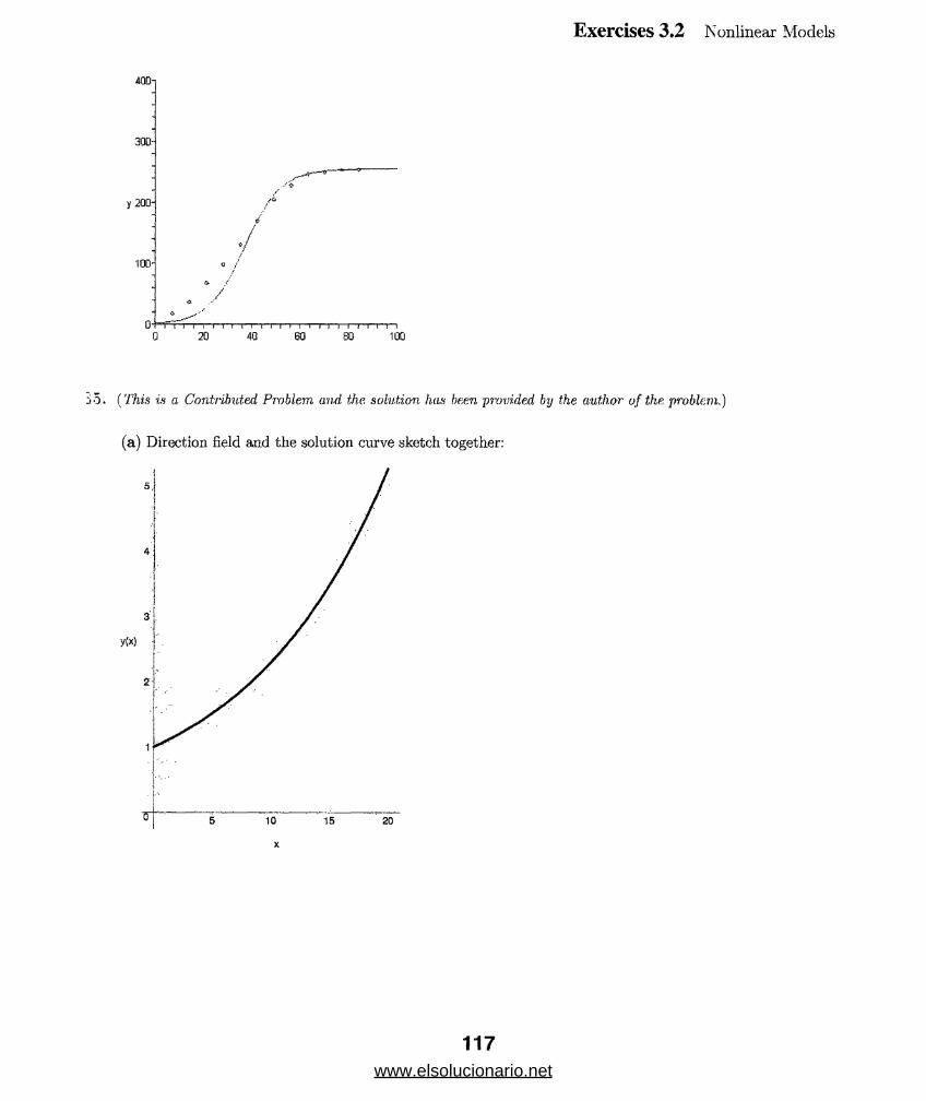
Exercises 3.2 Nonlinear Models
>5. (This is a Contributed Problem and the solution has been 'provided by the author' of the problem.)
(a) Direction field and the solution curve sketch together:
117www.elsolucionario.net

(b) The solution is P(t) — ekt, k = 1/12. with graph:
Exercises 3.2 Nonlinear Models
(c) the DE has the constant zero function as equilibrium.(d) The population grows to infinity.(e) If the initial population is Po then the resulting population would be P(t) = P0ekt,k = 1/12,(f) The solution would change from constant to exponential.(g) Direction field with solution sketch.
118www.elsolucionario.net
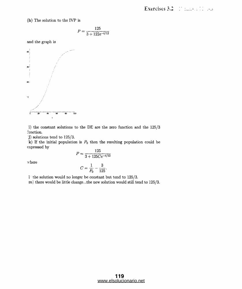
Exercises 3.2
(h) The solution to the IVP is
125P =
3 + 122e-{/12
and the graph is
c ao 4o
i) the constant solutions to the DE are the zero function and the 125/3 function.j) solutions tend to 125/3.k) If the initial population is Po then the resulting population could be
expressed by125
P =3 + l25Ce~f/12
inhere= JL
Po 125'
1 the solution would no longer be constant but tend to 125/3.m) there would be little change...the new solution would still tend to 125/3.
119www.elsolucionario.net
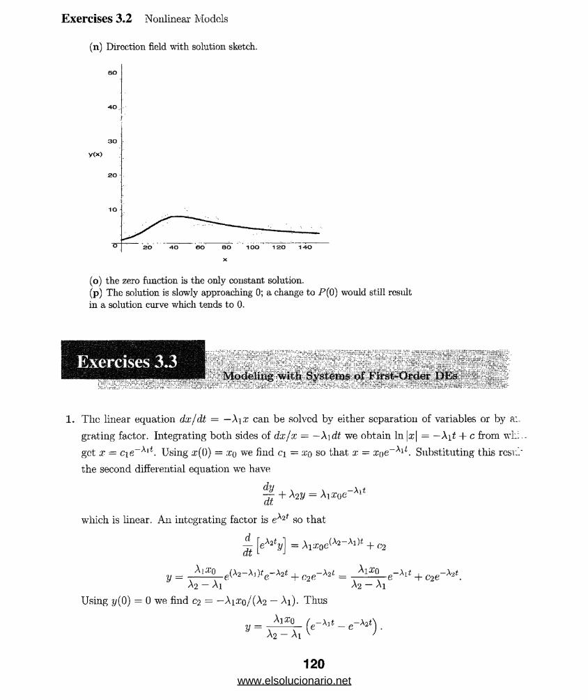
(n) Direction field with solution sketch.
50
Exercises 3.2 Nonlinear Models
40
(o) the zero function is the only constant solution.(p) The solution is slowly approaching 0; a change to P(0) would still result in a solution curve which tends to 0.
• r.
„„ " ; J 5 w'v - :y- ~
*'*:'! -'!; " '-11 : yi „ ...<;; .
1. The linear equation dx/dt = —Xyx can be solved, by either separation of variables or by a:
grating factor. Integrating botli sides of dx/x = —X\dt we obtain In |x| = —X\t + c from wh:
get x — cie_A|t. Using ;r(0) = xq we find ci = xo so that x = xoe~XlL. Substituting this resr.
the second differential equation we have
dy
dt+ M y = Aiaroe Xlt
which is linear. An integrating factor is e^2t so that
_d
dteX2ty (A a -A i)* + C2
yAi.T0 3(A2 —Aj )tr>—\2t -A 2t-
A2 - Ai
Using y(0) = 0 we find C2 = — Aixo/(A2 — Ai). Thus
A2 — Ai
Ai#. C2e-A 2*
120www.elsolucionario.net
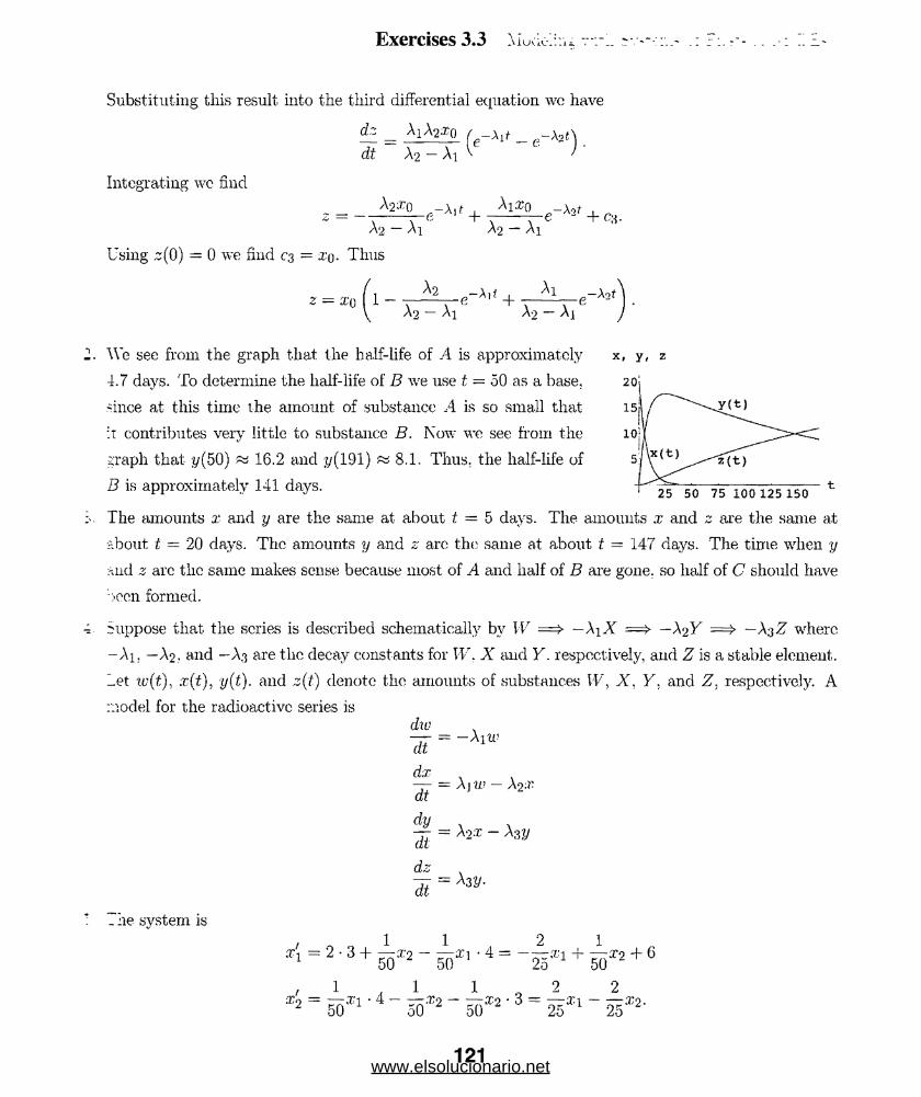
Exercises 3.3 Mudc-lr.i* ?--
dz _ A1 A2 .ro / Xlf _ -x2t\dt A2 -A 1 V' " ^
Integrating wc find
* = - J S t * - * * + + c;i.
Substituting this result into the third differential equation wo have
A2 — Ai
Using z(0) = 0 we find C3 — xq. Thus
A2 - Ai
A2 — Ai A2 — A]
We see from the graph that the half-life of A is approximately
4.7 days. To determine the half-life of B we use t = 50 as a base,
ince at this time the amount of substance A is so small that
:t contributes very little to substance B. Now we see from the
graph that y(50) « 16.2 and 2/(191) ~ 8.1. Thus, the half-life of
B is approximately 141 days.
The amounts x and y are the same at about t ~ 5 days. The amounts x and 2 are the same at
about t = 20 days. The amounts y and s arc the same at about t = 147 days. The time when y
and 2 arc the same makes sense because most of A and half of B are gone, so half of C should have
>ocn formed.
Suppose that the scries is described schematically by W = > — XiX = > —A2Y =>■ —A3Z where
-Ai, — A2, and —A3 are the decay constants for W. X and Y . respectively, and Z is a stable element,
let w(t), x(t), y(t). and z(t) denote the amounts of substances W, X , Y. and Z, respectively. A
model for the radioactive series isdw
m = - Ai“’
dx
dt= Aj w — X2 X
'he system is
<ty , »n = - X3V
dz
h = X z v -
/ = 2 - 3 4 = - ^ + 1 * 3 + 6i 1 1 1 1 , 2 2
= 50X1 • 4 “ 50*2 - 5012 • 3 = 25*1 ~ 2512'
•T
121www.elsolucionario.net

Exercises 3.3 Modeling with Systems of First-Order DEs
6. Let £]. X2 - and .7:3 be the amounts of salt in tanks A, B. and C, respectively, so that
1
100*
7. (a) A model is
ioo;/'2 • 2 -100:j=l*6 = ^ 2 - 3
50:tlToo2,1 •6 + iooa73- B o " 2 ’2 “ lOO 2 '
. 3O = --Xa -50 1 'I5o*2 +i i r 2 • 5 — 1
ioori.3 - • 4 1 _“ 20X2 “
1—X'3. 20dx 1
= 3- x2 0 Xl ®i(0) = 100dt 100 - 1 100 + 1'dx2 = 2- XI X2 *2(0) = 50.dt 100 + 1 ' 100 - t ’
(b) Since the system is closed, 110 salt enters or leaves the system and x i ( t ) + X 2( t ) = 100+50 = 1'
for all time. Thus x\ = 150 — x2 and the second equation in part (a) becomes
dx2 _ 2(150 - x2) _ 3x2 _ 300 _ 2x2 _ 3x2
dtor
100 + t
dx 2+
100 - t 100 + t 100 + 1 100 - t
3002 3+ x2 =
dt V100 + t 100 - t ) * 100-M ’
which is linear in x2. An integrating factor is
e 21n(100+t)-31n(100-t) = ^ q q + _ fyZSO
Adt
[(100 + i)z(100 - i)_;ix2] = 300(100 + i)(100 - 1)~3.
Using integration by parts, we obtain
(100 + i)2(100 - t)~*x2 = 300 ^(100 + i)(100 - t)~2 - -(100 - t)~l + c
Thus300
X2 =(100 + 1)2
300
c(100 - t f - ^(100 - t f + ^(100 + *)(100 - t)Z; Zi
- d o o + t ^ 1” -*) + 4(100- ‘M-
Using :c2(0) = 50 we find c = 5/3000. At t = 30, ,r2 - (300/1302)(703c + 30 • 70) w 47.4 11 -
8 . A model is
^ = (4 gal/min) (0 lb/gal) - (4 gal/min) ( ^ j * i lb/gal^
dx 2df = (4 gal/min) ( 7 ^*1 lb/gal) - (4 gal/min) ( ^ * 2 lb/gal
^ = (4 gal/min) ( ^ * 2 lb/gal) - (4 gal/min) ( ^ * 3 lb/gal)
122www.elsolucionario.net
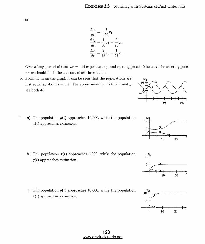
or
Exercises 3.3 Modeling with Systems of First-Order DEs
dx i 1
~W “ _ 50;)
dx 2 1 2
dt
£ISII
~ 75
dx 3 2 1
Ht = 75*2 “ 25
Over a long period of time wc would expect x\, X2 • and x$ to approach 0 because the entering pure
water should flush the salt out of all three tanks.
Zooming in on the graph it can be seen that the populations are
rlrst equal at about, t = 5.6. The approximate periods of x and y
•>.re both 45.
a) The population y(t) approaches 10,000, while the population
x(t) approaches extinction.
b) The population x(t) approaches 5,000, while the population
(/(/;) approaches extinction.
x,yk10--
5-
__10 20
The population y(t) approaches 10.000, while the population
x(t) approaches extinction.
*■>* 10
10H-- 1-- h
20
123www.elsolucionario.net
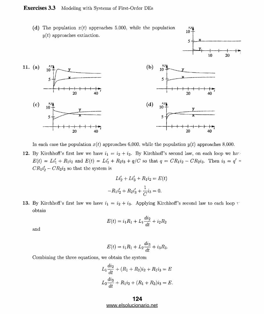
Exercises 3.3 Modeling with Systems of First-Order DEs
(d) The population x(t) approaches 5.000. while the population
y(t) approaches extinction.
x’yk 10
10 20
(b) 10-
5-b
20 40
<C) I?*!i
1 0 -y
5 - r
-L i
a
» i i i. 1 L w .t20 40
In each case the population x(t) approaches 6.000, while the population y(t) approaches 8.000.
12. By KirchhofFs first law we have i\ = i-2 + h- By KirchhofF’s second law, on each loop we hav
E(t) = Li[ + R \% 2 and E(t) = Li\ + + qjC so that q = CR\i-2 — CRzh- Then i$ = q' =
CRii .<2 — CR2h so that the system is
Li’2 R\i‘z ~ E(t)
—R\if2 + R‘2hi + ^*3 = 0.
13. By Kirchhoffs first law we have i\ = %2 + h- Applying Kirchhoff’s second law to each loop r
obtain
E(t) = i lR 1 + L)^ + i2R.2 at
and
E(t) = i1Ri + L2-£+isR3-
Combining the three equations, we obtain the system
L i—^ + (Ri -f R2)i2 + R\h = E
■2~7T + - 1*2 + (- 1 + - 3)*3 = E. at
124www.elsolucionario.net
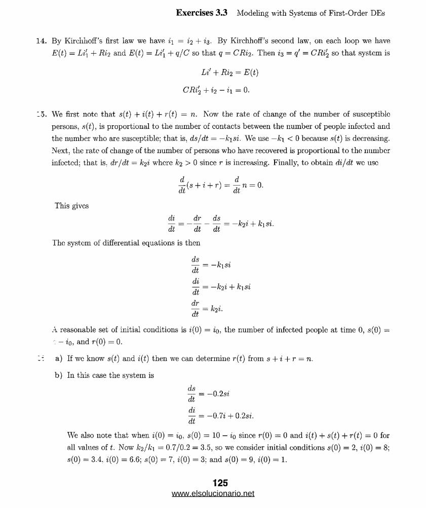
Exercises 3.3 Modeling with Systems of First-Order DEs
14. By KirehhofFs first law we have i\ = i<i + h- By KirchhofFs second law, 011 each loop we have
E(t) — Li\ + Rio and E(t) — Li[ + qfC so that q = CRi2. Then *3 = q' = CRif2 so that system is
Li1 + R i’2 = E(t)
CR'Iq t- 2 — 1 = 0.
15. We first note that s(t) + i(t) + r(t) = n. Now the rate of change of the number of susceptible
persons, .s(t), is proportional to the number of contacts between the number of people infected and
the number who are susceptible; that is, ds/dt = —k-isi. We use — k\ < 0 because s(t) is decreasing.
Next, the rate of change of the number of persons who have recovered is proportional to the number
infectcd; that is. dr/dt — k^i where k-2 > 0 since r is increasing. Finally, to obtain di/dt wc use
d / . n d_ ( s + ! + r) = _ r; = o.
This gives
di dr ds 7 .
i t = - J t - J t = -h t+ k ,s ’ •
The system of differential equations is then
ds ,
j t = ~h s '
di .1 — 12 I ST* dt
dr .
Tt = h l-
A reasonable set of initial conditions is i(0) = io, the number of infected people at time 0, s(0) =
— to? and r(0) = 0.
1* a) If we know s(t) and i(t) then we can determine r(t) from s + i + r = n.
b) In this case the system is
ds— = — 0.2s?, dt
di-- = —0.7i + 0.2 si. dt
We also note that when i(0) = io, s(0) = 10 — io since r(0) = 0 and i(t) + s(t) + r(t) = 0 for
all values of t. Now fo/fci — 0.7/0.2 = 3.5, so we consider initial conditions s(0) = 2, i(0) = 8;
,s(0) = 3.4, i(0) = 6.6; s(0) = 7, i(0) = 3; and a(0) = 9, i(0) = 1.
125www.elsolucionario.net
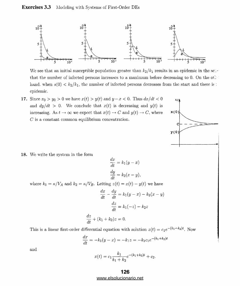
Exercises 3.3 Modeling with Systems of First-Order DEs
Wc see that an initial susceptible population greater than A'a/A'i results in an epidemic in the se:
that the number of infected persons increases to a maximum before decreasing to 0. On the ot;
hand, when .s(0) < fo/A'i, the number of infected persons decreases from the start and there is
epidemic.
17. Since xo > yo > 0 we have x(i) > y(t) and y — x < 0. Thus dx/dt < 0 *,>•*
and dy/dt > 0. We conclude that x(i) is decreasing and y(t) is
increasing. As t —> oc we expect that x(t) —* C and y{i) —> C, where x(° V
C is a constant common equilibrium concentration. cy(0)
18. We write the system in the form | - ‘■to-.)where k\ - k/Va and k-2 — k/Vb• Letting z{t) = x(t) — y(t) we have
ft = h{~Z) ” hZ— -t- (ki + ^2 )z — 0.
This is a linear first-order differential equation with solution z(t) = . Now
^ = - fa(y - x) = -k\z = -fcicie"(*1+fc2)*
and
X ( t ) = Cl e ~ ( k^ + k^ )1 -)- co.k i + k-2
126www.elsolucionario.net

Exercises 3.3 Modeling with Systems of First-Order DEs
Since y(t) = x(t) — z(t) wc have
y(t) = -ci-k'2 (/.'l+AroU
ki + A’2
The initial conditions ;r(0) = x q and y ( 0) = yo imply
C9-
Ci = X q
The solution of the system is
x{t)
yo and c2 =
fa) ~ Vo)h „ -(k hi + h’2
{ki+k2)t- +
v(t) =(yo - *o)k'2 _
+
Xf)k2 + yoki
k\ + A’2
xpk‘2 -j- ypki
ki + k'2
- yoh
k] + ko
As t —> oc, x(t) and y(t) approach the common limit
xoka + yoh xqk/Vb + jjqk/Va
k\ + k’2
x q V a + y o V n
ki + k-2 k/Va + k/Vb
Va
Va + VB
+yo77VB
x l&30 -
i
20 -- \ x l
10 - ^ * 2i— t— r t i — r t i t i
50 100
Va + Vb Va + VB
This makes intuitive sense because the limiting concentration is seen to be a weighted average of
the two initial concentrations.
Since there are initially 25 pounds of salt in tank A and
none in tank B, and since furthermore only pure water is
'.eing pumped into tank A, we would expect that xi(t)
~ould steadily decrease over time. On the other hand.
'■’ice salt is being added to tank B from tank A, we would
xpect X2 (t) to increase over time. However, since pure
"“ftter is being added to the system at a constant, rate and
- mixed solution is being pumped out of the system, it makes sense that the amount of salt in both
‘ .•:iks would approach 0 over time.
” •> assume here that the temperature, T(t). of the metal bar does not affect the temperature, TA(t).
.: ihe medium in container A. By Newton's law of cooling, then, the differential equations for T^t)
■:.:i T(t) are
^ = kA(TA - Tli), kA < 0
f = W - T a ), * < 0,
;ect to the initial conditions T(0) = Tq and TA(0) = TV Separating variables in the first
v.i'ition. we find T'A(t) = Tq + ciek’At. Using 7^(0) = T\ wc find c\ = Ti — TB, so
TA(t) = TB + (Ti - TB)ek-*1.
127www.elsolucionario.net

Exercises 3.3 Modeling with Systems of First-Order DEs
Substituting into the second differential equation, we have
^ = k(T - Ta) = kT - kTA = kT~ k[TB + (Tx - TB)ek }
d T — - kT = -kTB - k(T\ - TB)eM.
This is a linear differential equation with integrating factor e-/ “ kdt = e~kt. Then
~[e 'klT) = -kTBe 'kt - k{Ti - TB)e^A~k> at
e~ktT = TBe~kt - 7—^ - ^ - TB)e kA~k)t + c2k-A - k
T = Tb - - TB)ekAt + c2ekt.k.A - k
Using T(0) = To wc find c-2 = To - Tb + ——— (?i - Tg), sok-A - k
T(t) =T b - -— r(7i - TB)ekAt +k-A. —
7h-T c + - i- T(T1 - r s )A ; 4 — k
ekt.
21. (77ws is a Contributed Problem and the solution has been provided by the authors of the problem.)
(a) In the short term there is a mixing of an ethanol solution. In the long term, the system will contain a 20% sohition of ethanol.
(fa)100P" = — P - --Q - P1
50 10^
(c) First write Q = 50P'—30+P/2 and then it’s straightforward substitution into the equation in (b).
(d) From equation in (19) we find P'(0) = 6/10 + 7/50 — 200/100 = —63/50. The solution is
p (t) = e“t/400 s i n ( )\/95 - 100e-^40°cos(|^) + 100
(e) The solution is
m + 20 +(f) In both cases, the there is a concentration of 20% in each tank; P(t) —» 100 and Q(t) —» 20.
128www.elsolucionario.net
Chapter 3 in Review
I. The differential equation is dP/dt — 0.15P.
True. From dA/dt — kA. .4(0) ■ Aq, we have A(i) = A$ekt and A'(t) — kAoekt, ho .4/(0) = kA^.
At T = -(In 2)*.
I. irrom — = 0.018P and P(0) — 4 billion wc obtain P = 4e0018i so that P(45) = 8.99 billion. dt
4. Let A = A(t) be the volume of CO2 at time t. From dA/dt = 1.2 — A/4 and A(0) = 16 ft3 we
jbtain A = 4.8 + 11.2<?-i/4. Since A(10) = 5.7 ft3, the concentration is 0.017%. As t —> 00 we have
.4 -»• 4.8 ft3 or 0.06%.
Separating variables, we have
A'(-(\n2)/k) = M(-(ln2)/Jfc) = kA()ek hl2^'^ = k.A0erln2 = ^kAQ
y
Substituting y = s sin 6, this becomes
\js2 — s2 sin2 0(s cos 9)dQ = —dx
s sin 6
s
s In | csc 9 + cot 0\ + s cos 6 — —x + c
y/s2 - y 2' yj s2 — y2------ + s ------ = — X + c.= —x + c.
y y
Letting s = 10, this is
-10 hi -
129www.elsolucionario.net

Chapter 3 in Review
Letting x = 0 and. y = 10 wc; determine that c. = 0, so the solution is
10+ ^/100- 1,2 /— — -----*------- + ^/100 - y2 = -x
or
-10 In
x = 10 In
y
lo + yioo” r\/l00 - y2.
6. From VdC/dt = kA(C, - C ) and C(0) = C0 we obtain C = Ca + (Co - Cs)e~kAt/v.
7. (a) The differential equation
l- = k(T- Tm) = k[T - T2 - BIT, - T)]
= i[(l + B)T - (BTi + r 2)] = *(1 + b ) ( t - — ^ f 2)
is autonomous and has the single critical point (BT\ + T2)/(l + B). Sincc k < 0 and B
by phasc-linc analysis it is found that the critical point is an attractor and
BT\ + T2lim Tit) = t^oo w 1 + B
Moreover.
lim Tm(t) = lim [T2 + B(Ti - T)] = T2 + B (t, -t—>OC t—>OC \ 1 -1- £>BTi + T2
B
(b) The differential equation is
(IT
dt= k(T - Tm) = k(T -T2 ~ BTi + BT)
ordT— - k( 1 + B)T = —k(BT\ + T2).(/• 6
This is linear and has integrating factor e~ f K1+-D)dt _ e-k{i+B)i Thus,
y[e_&(1+s^T] - -k(BTi+T2)e-k<1+BU (
& J " 1 + J? 6 ' 6
T(i) = + cek{'+B)t.
Since k is negative, lim^oc T(t) = (BT\ -f 2^)/ ( l + B).
(c) The temperature T(t) decreases to the value (BT\ + T2 )/(l + B), whereas Tm(t) incrcas.
(BTi+T2)/(1 +B) as t —► oc. Thus, the temperature {BT\ +T2)/{1 + B), (which is a. wei<_.
average
B Ti + — l— T21 + B 1 + B
130www.elsolucionario.net
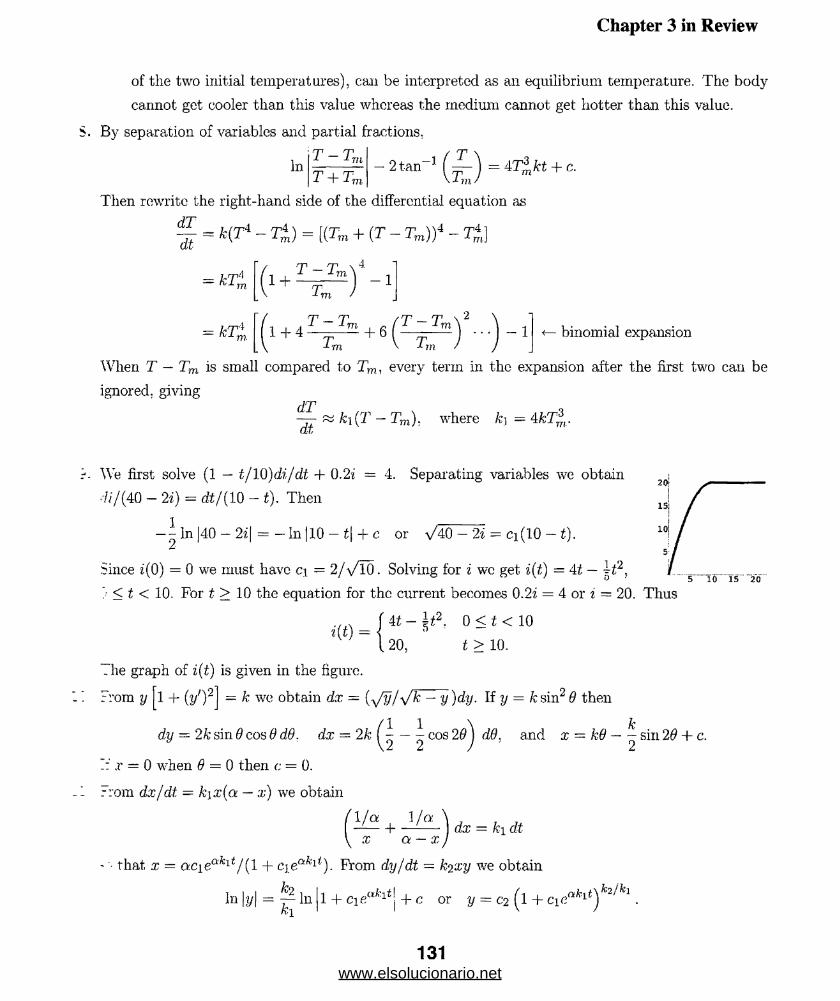
Chapter 3 in Review
of the two initial temperatures), can be interpreted as an equilibrium temperature. The body
cannot get cooler than this value whereas the medium cannot get hotter than this value.
S. By separation of variables and partial fractions.
In'-rnt - t,;
T + Tm
Then rewrite the right-hand side of the differential equation as
- 2tan 1 ( — ) = 4T^kt + c.
dT~ = k(T* - T4) = [(Tm + (T - Tm) f - T4 ]dt
= kT:rn 1 +Tn
\ + i ^ k + 6 ' t ~ t 'm
2- 1 binomial expansion
-Lm \ * 771
When T — Tm is small compared to Tm, every term in the expansion after the first two can be
ignored, givingdT- & h ( T - Tm). where fci = AkT* .at
We first solve (1 — t/10)di/dt + 0.2i = 4. Separating variables we obtain
■7/'/(40 — 2i) = dt/(10 — t). Then
— - In 140 — 2i\ = — In 110 — + c or y/AO — 2% - ci(10 — t).
Since i(0) = 0 we must have c\ -- 2/\/l0. Solving for i wc get i(t) = At — I t2,
■,* f 4 t - U . 0 < t < 1 0z(t) = < a '
I 20, t > 10.
The graph of i(t) is given in the figure.
From y 1 + (y')2 - k we obtain dx = (■s/y/y/k — y)dy. If y = A: sin2 9 then
dy = 2k sin 9 cos 9 d-9. dx = 2k Q — ^ cos 29j d9, and x = k9 — ^ sin 29 + c.
I: ,r = 0 when 9 = 0 then c = 0.
Trom dx/dt. — k\x(a — x) we obtain
/ 1/a + J / a \ ^ =
\ x a — x J
- '■ that, x = Q.cieaklt/ (I + cj eQ&l/). From dy/dt = k^xy we obtain
k-2In |y| = ~ In |l + cieakltj +c or y = c2 ( l + cie"*1*)*2' ** .
131www.elsolucionario.net

Chapter 3 in Review
12. In tank A the salt input is
v mm J \ gal J \ rainy'x2_ _lb ''
100 gal
i i . 1 \ lb
100 J min
The salt output is
f i l M - ( 5 &L) ( i l = A . .J min J y 100 gal j + \ min J \100 gal J 25 *1 min
In tank B the salt input is
The salt output is
B f i lnun,
' Jb_\
,100 galj
lb
20 min
gal \ ( X2 lb
min/ 1100 galH- 4
gal
min J V100 gal J 20 inin
x2 lb \ 1 lb— r = ™ x2
The system of differential equations is then
dxi 1 2
- M = 1 4 + m X2-25* '
dX'2 1
~dt
1
20 X l 20 a’2 '
13. From y = —x — 1 + c\ex we obtain 1/ = y -f x so that the differential equation of the ortho,t
family is
dy 1 dx-f- = -- — or —~+x = -y.dx y + x dy
This is a linear differential equation and has integrating factor e-ldy — ey, so
Tv [e"x] = ~ve’
eyx = —yev + ey + C2
x = — y + 1 + C2?~v-
132www.elsolucionario.net
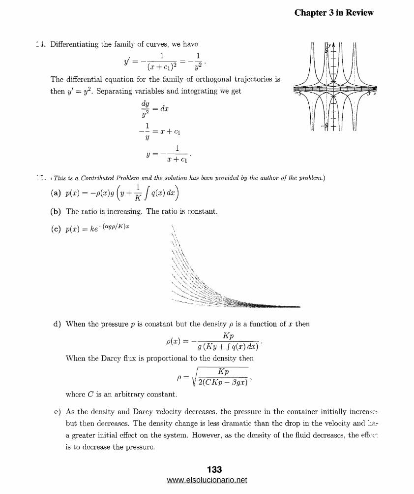
Chapter 3 in Review
.4. Differentiating the family of curves, we have
1V
(x + ci)2 y2 '
The differential equation for the family of orthogonal trajectories is
then y' ~ y~. Separating variables and integrating we get
r
i----- = X + Cl
y
ly = X + Cl
This 'is a Contributed Problem and the solution has been provided by the author of the problem.)
1(a) p(x) = -p(x)g ( y + x j Q(x) dx]
(b) The ratio is increasing. The ratio is constant.
(c) p(z) = \
1 .VWx\\\\\
ft*
d) When the pressure p is constant, but the density p is a function of x then
/ x ________ Kp
P[X) 9 (Ky + f q(x) dx) ’
When the Darcy flux is proportional to the density then
p = \!Kp
V 2{CKp - 3gx) '
where C is an arbitrary constant.
e) As the density and Darcv velocity decreases, the pressure in the container initially increase-
but then decreases. The density change is less dramatic than the drop in the velocity and lias
a greater initial effect on the system. However, as the density of the fluid decreases, the effec:
is to decrease the pressure.
133www.elsolucionario.net

Chapter 3 in Review
S i>5 -
im
0.95 “
GM -
J ----1— 1----I— !----i— (----L . A I. t > I 1 1 I__ i----»—1 » » * » * < 1 <I 2 S 4 5 A
1 6 . ( T /iis is a Contributed Problem and the solution has been provided by the authors of the problem.)
(a) D irection fie ld and the solution curve sketch together: (b) The solution is P (t) — efci\ k = 1/12, w ith graph:
(c) the JDE lias the constant zero function as equilibrium .(d) The population grows to in fin ity.(e) I f the in itia l population is Po then the resulting population would be >(t)^P0e^A;-l/12,(f) The solution would change from constant to exponential.
134www.elsolucionario.net
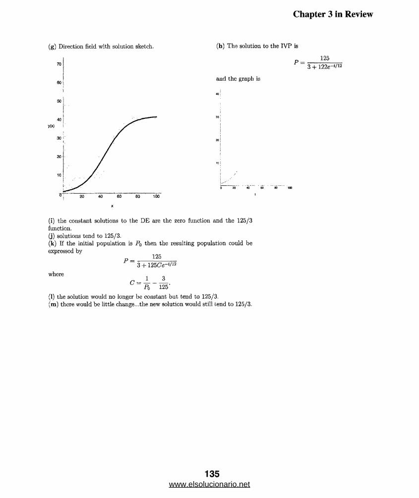
Chapter 3 in Review
(g) D irection field w ith solution sketch.
70
601
(h ) The solution to the IV P is
P =
and the graph is
125
0 20 4C SO 80 100
(i) the constant solutions to the DE are the zero function and the 125/3 function.(j) solutions tend to 125/3,(k ) I f the in itia l population is Pq then the resulting population could be expressed bv
125
where
3 + 1 25C'e-£/J2
Po 125-
(1) the solution would no longer be constant but tend to 125/3.(m ) there would be little change...the new solution would s till tend to 125/3.
135www.elsolucionario.net

Chapter 3 in Review
(n) Direction field with, solution sketch*
(o) the zero function is the only constant solution.(p) The solution is slowly approaching 0; a change to P(0) would s till result in a solution curve which tends to 0,
136www.elsolucionario.net
4 Higher-Order Differential Equations
1 rrom y — c\ex + C2 e x we find y' = ciex — c-ie x. Then y(0) = c\ + C2 = 0, y'(0) ~ c.\ — oi = 1 so
_:iat c\ — | and c-2 = The solution is y = ^ex — \e~x.
I From y = cielx + c.2 e~x we find y' ~~ 4cif;4x — C2e-X. Then y(0) = c\ + 0 2 = 1. ;t/(0) = 4ci — c*2 = 2
that- ci = | and oi = §. The solution is y = le4* + ge-*.
:. From y = c\x + C2X In ® we find y' - ci + C2(l + In a?). Then y(l) = Ci = 3, y'(l) = c\ + C2 = — 1 so
‘hat ci = 3 and C2 ‘ —4. The solution is y = 3x — Ax In a;.
4. 7:om y — a + oi cos x + C3 sinx we find y' — —oi sinx 4- c$ cos x and y" — —C2 cos x — C3 sin®. Then
. :r) = ci - C2 = 0. y'(7r) = — C3 — 2, it/'(7r) — C2 = -1 so that ci = -1. C2 = -1, and C3 — -2. The
i:-lution is y = — 1 — cosx — 2sin®.
! From y = c 1 + cjx2 we find y' = 2c9®. Then y(0) = ci = 0, 2/ (0) = 2c2 -0 = 0 and hence y'(0) = 1
i' not possible. Since 02(2:) = x is 0 at x = 0, Theorem 4.1 is not violated.
: In this case we have y(0) = c\ = 0, y'{0) — 2c2 • 0 = 0 so ci = 0 and C2 is arbitrary. Two solutions
:-:e y = x2 and y = 2x2.
From ®(0) = ®o = ci wc see that x(t) = .rocos urt + 02 sin art and x'{t) = -®o sin art + oivcoswt.
Then :c'(0) = ®i = C2ui implies 0 2 = ®i fu. Thus
, . ®i . x(t) = xq cos u>t H-- sm u>t.
U)
* ' jiving the system
x(to) = c\ cosutfo + 0 2 sin ujto — ®o
= — c i u ; s i n ^ o + c 2 u > c o s a t f o = x l
::r ci and C2 gives
ujxq cos ujt,Q — x\ sin cos u>to + coxq sin toto ci = ----------------- and C2 = -----------------.
UJ UJ
137
www.elsolucionario.net
Exercises 4.1 Preliminary Theory- Linear Equations
Thus. , cuxq c o s uito — £1 sin uto x’i cos ujIq + uixq sin u>to .
x[t) — -----------------cos u)t-\-------------------sin a;*to C0
Xy= xq (cos a)t cos u)t-o + sin cut sin u^o) ~i-- (sin uit, cos ojIq — cos tot sin coto)
= xq cos 'jj(t — to) + — sin(j(t — t-o).iO
9. Sincc (1 2 (x) = x — 2 and x'o = 0 the problem has a unique solution for — oo < x < 2.
10. Sincc o q ( x ) = tana; and xq = 0 the problem has a unique solution for —tt/2 < x < 7r/2.
11. (a) We have 7/(0) = c.\ + c2 - 0, y(l) - cie + C2 e~1 = 1 so that ci - ej (e2 — l)
C2 — —ej (e2 — l). The solution is y = e (ex — e-'*) / (e2 — l).
(b) We have y(0) = C3 cosh 0 + C4 smb. 0 = C3 — 0 and y(l) = 03 cosh 1 + c\ sinh 1 = C4 sinh 1 -
so C3 = 0 and 04 = 1 /sinh 1. The solution is y = (sinh x)f (sinh 1).
(c) Starting with the solution in part (b) we have
1 . , 2 ex — e~x ev - e~x e . _V — . : „ sinh x = ---- r -- --- = ----- 1— = -s---(e — e ).
smhl el — e-i 2 e —1/e e2 — 1
12. In this ease we have t/(0) = cj = 1. y'( 1) = 2c2 = 6 so that c\ ~ 1 and 0 2 = 3. The solutic
y = 1. + 3a:".
13. From y ~ aex cosx + c2ex sin a: wc find y' = cic!C(— sin a; — cos a?) + C2e*(cosa: + sinx).
(a) We have y(0) = c\ = 1, yj(ir) = —en(ci + c2) = 0 so that c\ = 1 and c2 — —1. The solutic:.
y = ex cos x — ex sin x.
(b) We have y(0) = c\ = 1, j/(tt) = — ex = —1, which is not possible.
(c) We have y(0) = c\ = 1, y(iif2) = C2e7r/2 = 1 so that ci = 1 and 0 2 = e_7r/2. The solutic:.
y — cx cos x + e_7r/2ex sin x.
(d) We have (0) = c\ = 0. y(it ) — C2e7rsiii7r = 0 so that c\ = 0 and C2 is arbitrary. Solutions
y = c2ex sin a:, for any real numbers C2 .
14. (a) We have y(—1) = cy + c2 + 3 = 0, ty( 1) = c\ + 0 2 + 3 = 4, which is not possible.
(b) We have y(0) = ci ■ 0 + c2 • 0 + 3 = 1, which is not possible.
(c) We have y(0) = c\ ■ 0 + C2 • 0 + 3 = 3, y(l) = ci + 0 2 + 3 = 0 so that c\ is arbitrary
c2 = —3 — c\. Solutions are y = c\x2 — (ci + 3)x4 + 3.
(d) W7c have ;</(!) = c\ + C2 + 3 = 3, y(2) = 4ci + I 6C2 + 3 = 15 so that c\ = —1 and c2 = 1. -
solution is y = —x2 + :r4 + 3.
15. Since (—■4)a: + (3)x2 + (l)(4:r — 3;c2) = 0 the set of functions is linearly dependent.
138www.elsolucionario.net
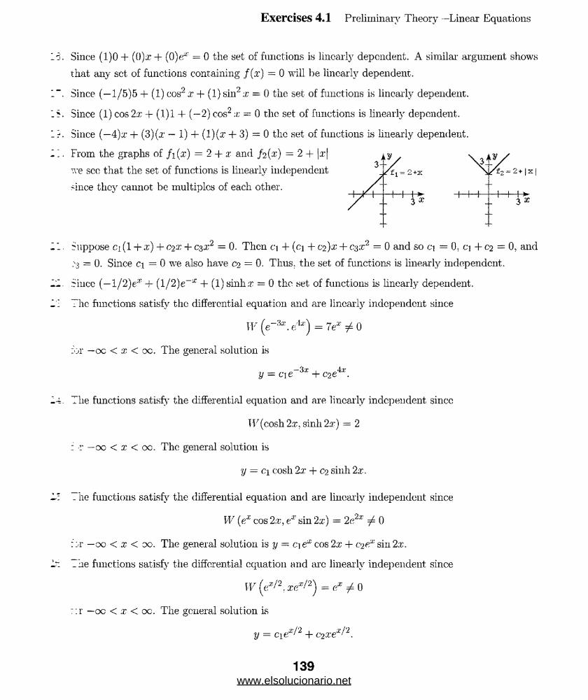
Exercises 4.1 Preliminary Theory -Linear Equations
Since (1)0 + (0)x + (0)e;<: = 0 the set of functions is linearly dependent. A similar argument shows
that any set, of functions containing /(:r) = 0 will be linearly dependent.
Since (1) cos2;r + (1)1 + (—2) cos2 x = 0 the set of functions is linearly dependent.
Since (—4)x + (3)(x — 1) + (l)(a~ + 3) = 0 the set of functions is linearly dependent.
Suppose ci (1 + x) + C2 X + csx2 = 0. Then ci + (ci + cz)x + c-sx2 = 0 and so ci — 0. ci + c-2 — 0, and
.•3 = 0. Since ci = 0 we also have C2 = 0. Thus, the set of functions is linearly independent.
Since (—l / 2)e;<! -I- ( l/2)e-x + (1) sinh.r = 0 the set of functions is linearly dependent.
The functions satisfy the differential equation and are linearly independent since
The functions satisfy the differential equation and are linearly independent, since
Hr(cosh 2.t\ sinh 2x) = 2
: r — 00 < x < oc. The general solution is
y = ci cosh 2x + a sinh 2x.
The functions satisfy the differential equation and are linearly independent since
W (ex cos 2.7;, ex sin 2x) = 2e2x 0
::r —00 < x < oc. The general solution is y = ci e‘t: cos 2a; + C2 PX sin 2x.
The functions satisfy the differential equation and are linearly independent since
Since (—1/5)5 + (1) cos2 x + (1) sin2 x = 0 the set of functions is linearly dependent.
From the graphs of fi(x) = 2 + x and fiix) — 2 + |ar|
we see that the set of functions is linearly independent
>ince they cannot be multiples of each other.
for — oc < x < oc. The general solution is
::r — oc < x < oc. The general solution is
y = Cl( ^ 2 + c2xex/'2.
139www.elsolucionario.net
Exercises 4.1 Preliminary Theory—Linear Equations
27. The functions satisfy the differential equation and are linearly independent, since
W (x3, xd) = x6 + 0
for 0 < x < oc. The general solution on this interval is
y = cix3 + C2 X1.
28. The functions satisfy the differential equation and are linearly independent since
W (cos (lnx). sin (lnx)) = 1/x ^ 0
for 0 < x < oo. The general solution on this interval is
y = ci cos(lnx) + C2 sin(lnx).
29. The functions satisfy the differential equation and arc linearly independent since
W (x, x~2,x~2 lnx) = 9x-6 7 0
for 0 < x < oc. The general solution on this interval is
_n _ny = ci x + c2x_ + C3X lnx.
30. The functions satisfy the differential equation and are linearly independent since
W (l, x, cos x, sinx) = 1
for - 00 < x < 00. The general solution on this interval is
y = ci + C2X + C3 cos x + c-i sin x.
31. The functions yi = a2x and ij2 = e5* form a fundamental set of solutions of the associated home. -
neous equation, and yp - 6ex is a particular solution of the rionbomogeneous equation.
32. The functions y\ = cosx and ij2 = sinx form a fundamental set of solutions of the associated ho:. ■
geneous equation, and yp = x sinx + (cosx) ln(cosx) is a particular solution of the nonhomogene,
equation.
33. The functions y\ = e2x and ys = xe2x form a fundamental set of solutions of the associr
homogeneous equation, and yp — x2e2x + x — 2 is a particular solution of the nonhomogent
equation.
34. The functions tji = x-1/2 and ij2 = x-1 form a. fundamental set of solutions of the associ;-'
homogeneous equation, and yp — j=x2 — |x is a particular solution of the nonhomogeneous equat:
35. (a) We have y'pi = 6e2x and y"} = 12e2x, so
ypi y'pi "I” Vpi. = 12eja" — 36e2x + 15e2'1 = —i)€2x.
140www.elsolucionario.net
Exercises 4.1 Preliminary Theory—Linear Equations
Also. y'po — 2x + 3 and y" — 2. so
y'p2 ~ 6 Vp2 + -5 yP2 — 2- 6(2;r + 3) + 5(x2 + 3x) = 5x2 + 3x - 16.
(b) By the superposition principle for nonhomogeneous equations a particular solution of
y" — 6]/ + 5y = 5x2 + 3a’ — 16 — 9e2x is yp = x2 + 3.x + ?>e2x. A particular solution of
the second equation is
Up = -2yP2 - - -2x2 - Gx - ^e2x.
(a) yPl = 5
(b) yP2 = —2x
(c) yP = Up I + yP2 = 5 - 2x
(d) yP = \yPx - 2yP2 - § +■ 4x
(a) Since D 2x = 0. x and 1 are solutions of y" = 0. Since they arc linearly independent, the
general solution is y = c^x + c%
(b) Since. DAx2 = 0. x2, x, and 1 arc solutions of y'" ■- 0. Since they are linearly independent, the
general solution is y = cix2 + c^x + <?:{.
(c) Since D 4x a — 0, X s . x2, x. and 1 are solutions of y(-4> = 0. Since they are linearly independent,
the general solution is y — c\ + 0 2 x2 + c$x + C4.
id) By part (a), the general solution of y" = 0 is yc = c\x + 0 2 - Since D2x2 = 2! = 2, yp = x2 is a
particular solution of y" = 2. Thus, the general solution is y = cyx + C2 + x2.
ie) By part (b). the general solution of y"' — 0 is yc = cyx2 + c^x + C3. Since D3x3 = 3! = 6,
yp = x'3 is a particular solution of y'" — 6. Thus, the general solution is y — cyx2+c2 x+cs +x3.
(f) By part (c), the general solution of = 0 is yc = c i a r * + C 3X+C4. Since DAx4 = 4! = 24,
yp - x4 is a particular solution of y ^ = 24. Thus, the genera,1 solution is y = cix3 + C2 X2 +
C3X + C4 + x4.
By the superposition principle, if ij] = ex and ij2 = e~x are both solutions of a homogeneous linear
■.'ifferential equation, then so are
www.elsolucionario.net
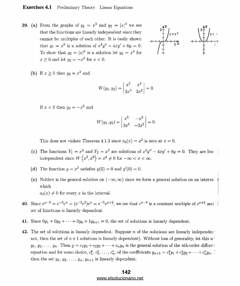
Exercises 4.1 Preliminary Theory Linear Equations
39. (a) From the graphs of y\ = .r5 and y-2 = we see
that the functions are linearly independent sincc they
cannot be multiples of each other. It is easily shown
that yi = x3 is a solution of x2y" — 4xy' + 6y = 0.
To show that y-2 = is a solution let y2 = x3 for
x > 0 and let y-2 = —x* for x < 0.
(b) If x > 0 then y2 = and
xW{yi ,y2) = \I 3ar
x-
3x2
i3-
t * i ,
? !- j y=x3
J\ 1 1 w7i \ r 1 3*
/ -/ -
= 0 .
If a: < 0 then y2 — — x* and
-:r3= 0.
3a,’2 — 3x2
This does not violate Theorem 4.1.3 since a2(x) = x2 is zero at x - 0.
(c) The functions Yi = x'* and Y2 = x2 arc solutions of x2y" — 4xyf + 6y — 0. They are line ]
independent sincc W (.r3, :r2) — :c4 ^ 0 for —oo < x < oo.
(d) The function y = x:i satisfies y(0) — 0 and //(0) = 0.
(e) Neither is the general solution on (—oo, oc) since we form a general solution on an interva.:
which
a2(x) ^ 0 for every x in the interval.
40. Sincc e1-3 = e~'iex = (e~°e2)ex — e~5ex+2, we see that ex~* is a constant multiple of ex+2 and '
set. of functions is linearly dependent.
41. Since 0-j/i + ()y2 H--- 1- 0j/k + lyt+i = 0, the set of solutions is linearly dependent.
42. The set of solutions is linearly dependent. Suppose n of the solutions are linearly independei:’
not. then the set of n +1 solutions is linearly dependent). Without loss of generality, let this sr
yi, i/2 • • • • ; yn- Then y = c\y\ -f- c2y2 H--- 1- CnVn is the general solution of the nth-order differe:/
equation and for some choice, cf, c2, . . . , c*. of the coefficients yn+i = cfyi + c2y2 H--- 1- c*yn. .
then the set y\, y2, . . . , yn, yn+i is linearly dependent.
142www.elsolucionario.net

Exercises 4.2 Reduction of Order
Reduction o f Order
Problems 1-8 we use reduction of order to find a second solution. In Problems 9-16 we use formula
' from the text.
1. Define y = u(x)e2x so
y' = 2ue2x -j- u'e2x, y" — e2xu" + Ae2xu' + Ae2xu. and y" ~ Ay'+ 4y = c2xu" = Q.
Therefore u" = 0 and u = c±x + c-2 - Taking c\ = 1 and c<i — 0 wc see that a second solution is
— ze .
Define y = u(x)xe~x so
y' = (1 — x)e~xu + xe~xu', y" = xe~xu" + 2(1 — x)e~xu’ — (2 — x)e~xu,
Hiid
y" + 2y' + y — e~'x(xu" + 2 u') = 0 or u" + ^ v! = 0.
2w — u! we obtain the linear first-order equation w' H— w — 0 which has the integrating factor
Jb,2fdx/x= x 2' Now
— = 0 gives x2w = c.d,x
Therefore w = it' = c/x2 and u = c\/x. A second solution is ih = —xe~x = e~x.x
- Define y = u(x) cos Ax so
y = —4 u sin 4x + u! cos 4x. y" = u" cos 4x — 8 u! sin 4x — 16u cos 4x
-::.d
y" + 16y = (cos 4x)u" — 8(sin4 x)v! = 0 or u" — 8(tan Ax)u' = 0.
I: iv = u! we obtain the linear first-order equation w' — 8(tan 4:r)'u; = 0 which has the integrating
:.-:Tor lan dx = cos2 4;c. Now
y- [(cos2 4x’)w] = 0 gives (cos2 4x)w = c.C/.X
Tiierefore w = u' = c sec2 4:c; and u — c\ tan4:r. A second solution is y<2 = tan Ax cos Ax ~ sin 4.x.
■r I -fine y = u(x) sin 33? so
y1 = 3 u cos 3x + u! sin 3x, y" = u" sin 3x + Qv! cos 3x — 9w sin 3.x.
143www.elsolucionario.net

Exercises 4.2 Reduction of Order
and
y" + 9y = (sin 3x)un + 6 (cos 3 z)v! = 0 or u" + 6(cot 3 x)u' = 0.
If w = u' we obtain the linear first-order equation w1 + 6 (cot 3x)w ~ 0 which has the integrati:..
factor e(i J cot'ixdx = sin2 3x. Now
- -[(sin2 3x)w] — 0 gives (sin2 3.t)m-! = c.
Therefore w = v! = ecsc2 3.x and u = c\ cot 3.x. A second solution is y-2 = cot 3x sin 3a: = cos 3x.
5. Define y = u(x) cosh x so
y' = u sinh x + u' cosh x, y" = u" cosh x + 2u' sinh x u cosh x
and
y" — y = (cosh x)u" + 2(sinli x)u' = 0 or un + 2(tanh.r)u/ — 0.
If w = v! we obtain the linear first-order equation w' + 2 (tanh x)w = 0 which has the integrati:.-
factor e2 f Tanh x dx = cosh2 x. Now
[(cosh2 x)w\ - 0 gives (cosh2 x)w — c.LJLJb
Therefore w == u- — csech2 x and u = c tanh x. A second solution is t/2 — tanh a; cosh x = sinh x.
6. Define y = u(x)e0X so
y1 — 5 e5xu + e5xuf, y" = e5xu" + 10 e?xul + 25 eaxu
and
y" - 25y = (?x{u" + 10u') = 0 or u" + 10u' = 0.
If w = v! we obtain the linear first-order equation w1 + 10«; = 0 which has the integrating fac:e io f d x = e i 0x_ N o w
4~ [e10;rU’] = 0 gives e10xw = c. dx
Therefore w = uf = a?-10* and u = cie-10x. A second solution is y2 — e- ^x( x — ( ~ox,
7. Define y = u(x)e2x so
y — -e2x/3u — e2x''^ur. y" = + -e2xi'Aii' -1- |e2x'/3uO O i/
and
9y" - Yly + Ay = 9e2:c/V = 0.
Therefore u" = 0 and u = cyx + c-2 - Taking c\ = 1 and C2 = 0 we see that a second solution
ij2 = xc2*'1.
8. Define y ~ -u(x)ex so
y — ^ex u + ex u ' < y" = + ^ex 'iul + ^e:S/,5w
144www.elsolucionario.net

Exercises 4.2 Reduc"'..:: '1
Qy" + y' — y — ex/'i (6u/> + 01/) = 0 or u" + -v* = 0.
x = uf we obtain the linear first-order equation it/ + §tt! = 0 which has the integrating factor
. r 1 I dx = e'W<>, Now
4-[e5x/6w] = Q gives e ^ w = c.dx
Therefore w = ur = ce-5x/6 and u = cie_5;j:-/K. A second solution is 2/2 = e_ox/6ex/3 — e_x/2.
‘ .iTiitifying P(x) = —Ijx we have
4 f e - ^ - y ^ J 4 f l , 4l , ,2/2 = x J --- ~8--- = x j - dx = x In |x|.
second solution is y2 = x4 In |x|.
" -.-ntifying P(x) = 2/x we have
o r e~ o f — r 12/2 = ar j --- -j---dx = x j x dx — —-x .
A second solution is y2 = x-3.
I ntifying P(x) = 1/x wc have
w * = lnx/ = ^ ( " i ^ ) = _1-A second solution is y2 = 1.
! Gratifying P(x) = 0 we have
/-— f Odx / 1 \dx — x1,/2 lnx ) = -x!/2.
xtlnx)"5 V In x j
A second solution is y2 = xl,!'2.
Identifying P(x) = — 1/x we have
r e- J-dx./x r xy2 = x sin(lnx) / , 2 — -dx = xsin(lnx) / , 2 — -dx J x2snr(lnx) J x2 sm (In x)
= xsin(lnx) [ (hix) ^ [_ cot(lnx)] = — xcos(lnx).J x
A sccond solution is y2 = x cos (lnx).
’ :’:entifying P(x) = —3/x we have
/ g - J - 3 d x / x ~ ,^3—i-- 777:— - dx — x2 cos(lnx) / — '-7T7-,— r dx
x'1 cosJ(lnx) J x4 cos2 (lnx)
0 ,, . /“sec2 (lnx) , 9 /, \ /, \ 0 . N = x“ cos(lnx) I -------dx = x“ cos(lnx) tan(ln x) = x“ sm(ln x).
145www.elsolucionario.net

Exercises 4.2 Reduction of Order
A second solution is ij2 = x 2 sin (In a;).
15. Identifying P(x) - 2(1 + x ) j ( l - 2a; - x2) we have
e - / '2(1 -Hr)d x / { l —2x—x 2) (} n { \ - 2 X- . r 2)
1)2 = {X + 1 ) j - -------------, ---------------d x = (X + 1 ) j — ------- d x
= ( . + i ) /
( x + 1 ) 2
1 — 2a’ — x 2 (* + l)2
2 1
(a: + 1)>
dx = (x + 1) J{x + iy
- 1 d x
. x + 1— X = -2 - r- - x.
In1 + X
1 — X
— (x + 1)
A second solution is 1/2 = x2 + x + 2.
16. Identifying P(x) — —2xj ( l — x2} we have
y 2 = I e ~ f -2xdx/(i-a?)dx = je - H '- ^ d x = j Y ^ 2 d x = 1
A second solution is y2 = ln|(l + x)/(l — x)\.
17. Define y = u{x)e~‘2x so
y' - -2ue_2x + u'e~'2x, y" = i"e~2x - 4u'e~'2x + 4ue~2x
and
y" - 4y = e~2xu" - 4e“2:V = 0 or u" - 4v! = 0.
If w = it! wo obtain the linear first-order equation w' — 4w = 0 which has the integrating
e~4f dx = e~4x. Now
-~[e~4xw] = 0 gives e~4xw = e. dx
Therefore w — v! — ce4x and u — cieix. A second solution is y2 — e~2xe4x = e2x. We
observation that a particular solution is yp — —1/2. The general solution is
—2x , 2 r 1 y = cle + c2e —
18. Define y = u(x) ■ 1 soy' = u', y" = v" and y" + tj = u" + u = 1.
If w = u' we obtain the linear first-order equation w' + w = 1 which has the integrating
eJ dx = ex. Nowd_
d x [ex w] = e x g iv e s e x w = e x + c.
Therefore w = u' = 1 + ce x and u = x + e.\e x + r;2 . The general solution is
y = u = x + c\e~x + c2.
146www.elsolucionario.net

Exercises 4.2 Reduction of Order
Define y = ».(a:)eT so
y = u,(f -i-iiex. y" = u"ex + 2u'ex + uex
and
y" - 3y' + 2y = exu" - exu = 5e3*
If «; = u' we obtain the linear first-order equation w1 — w = 5e2;r which has the integrating factor
r~J dx = e~x. Now
= oex gives e~xw ~ 5e'1 + ci.dx
Therefore w — u' — 5e2x + C]_ex and u = |e2a: + cie,T -r C2- The general solution is
y = uex = ^e3x + cie2u: -i- c2ex. z
Define y = u(x)ex so
y> = uer + u'ex, y" = u"e* + 2u'ex + ue*
r.l'A
y" — 4 y1 + 3 y = e1:u" — exu' = x.
I: u: = v! we obtain the linear first-order equation wf — 2w ~ xe~x which has the integrating factorJ 2 , l x = e - 2x_ N q w
d r _0,. , _ ‘<-r • _ Ot 1 1 _ ‘ir- ~ ie w = ice g iv es c - J ' w — — - x e - - c -| c i . axL 3 9
Therefore it? = u' = —|rre_ ‘x' — $e~x + c\elx and u = xe~x + -j- C2fi2,r + C3. The general
-: ’ ittion is
y = uex = - a; + - + C2e3:p + £36*.O Ja I For mi constant, let y\ = emiX. Then y[ = ?niemiX and y'{ = mfe"11*. Substituting into the
differential equation we obtain
ay 1 + by[ + cy \ = amjemiX + bni\emiX + cemrx
= e,nix(aml + bmi + c) = 0.
Thus, yi = emi* will be a solution of the differential equation whenever + lmi\ + c = 0.
Since a quadratic equation always has at least one real or complex root, the differential equation
must, have a solution of the form y i = e n l l X .
b 1 Write the differential equation in the form
// b . cV +~V + -V = Q-.
a a
147www.elsolucionario.net
Exercises 4.2 Reduction of Order
p —b x /a
- (, m i x j e - { b l a ^ r 2 m \ ) x ^ x
1 em , x e - ( b / a ^ 2 m i )x (mi ± -b/2a)
and let. yi = emyX be a solution. Then a second solution is given by
b/a + 2mi
^ — (b/a—m i )x
b/a + 2m\
Thus, when m-j ^ —b/2a, a second solution is given by 1/2 - em'2'x where m2 = —b/a —
When m-i — —b/2a a second solution is given by
U2 = em'lX J dx - xenilX.
(c) The functions
sin a; = ~(ev:r — e iX) cos® = ^(ew + e lx)£ /■ z
sinh 2; = — e_;i;) cosh./: = ^ (ex + e~x)£ £
are all expressible in terms of exponential functions.
22. We have y[ — 1 and y'{ = 0, so xy'[ — xy\ -f yi = 0 — x + x — 0 and yi(x) — x is a. solution of :
differential equation. Letting y = u(x)yi(x) = xu(x) we get
y1 = xn!(x) + u(x) and y" = xu"{x) + 2u'{x).
Then xy" — xy' + y = x2u" + 2xu' — x2v? — xu + xu = x2u" — (x2 — 2x)u' = 0. If we make *.
substitution w = -u'. the linear first-order differential equation becomes x2wf — (x2 — x)w = 0. wh:
is separable:
d w / . 1 '|U'
- = ( l — — )dx x xJ
dx v x'
dw
w
hi w = x — In x + c
exW — C] — .
x
Then v' - ciex jx and u - c\ j exdx/x. To integrate ex/x we use the series representation for
148www.elsolucionario.net
Exercises 4.2 Reduction of Order
a second solution is
f c(J‘2 = xu(x) = C-\X j — dx
=ClX J s (x+1+1*2+kl3+" )dx = c ' x . l ( l + 1 + ^ x + h l 3 + " ) dx
=cKln x+x+w f3+m x3+"= C l( x lu x + x 2 + w / + W f i +
interval of definition is probably (0. oc) because of the lri;c term,
a Y\ c have y’ = y" = ex. so
xy" — (x + 1.0)y' -r 10y = xex — (x + 10)ea: + lOe* = 0.
and y — ex is a solution of the differential equation,
b i By (5) a second solution is
r e~ I p(x)dx (■ ef dx r e/(i+io.Ac)rfxV2 = V iJ --- J 2---dx = c?J - e2;), - dx = ex j --- ----- dx
r -r+lna;10 r= ex j -—^ — dx — ex J x10e~x dx
= ea;(—3,628,800 - 3,628.800a: - 1,814,400a:2 - 604,800a;3 - 151,200a:4
- 30,240a:5 - 5.040a:6 - 720x7 - 90a:8 - 10a:9 - x10)e~x
= -3,628,800 - 3,628,800a: - 1,814,400a;2 - 604,800a;3 - 151,200.x4
- 30,240a'5 - 5,040a;6 - 720a:7 - 90.r8 - 10.x9 - a:10.
1 10 1c) By Corollary (A) of Theorem 4.1.2. —— y2 — — xn is a solution.
101 ' ^ o nl
149www.elsolucionario.net
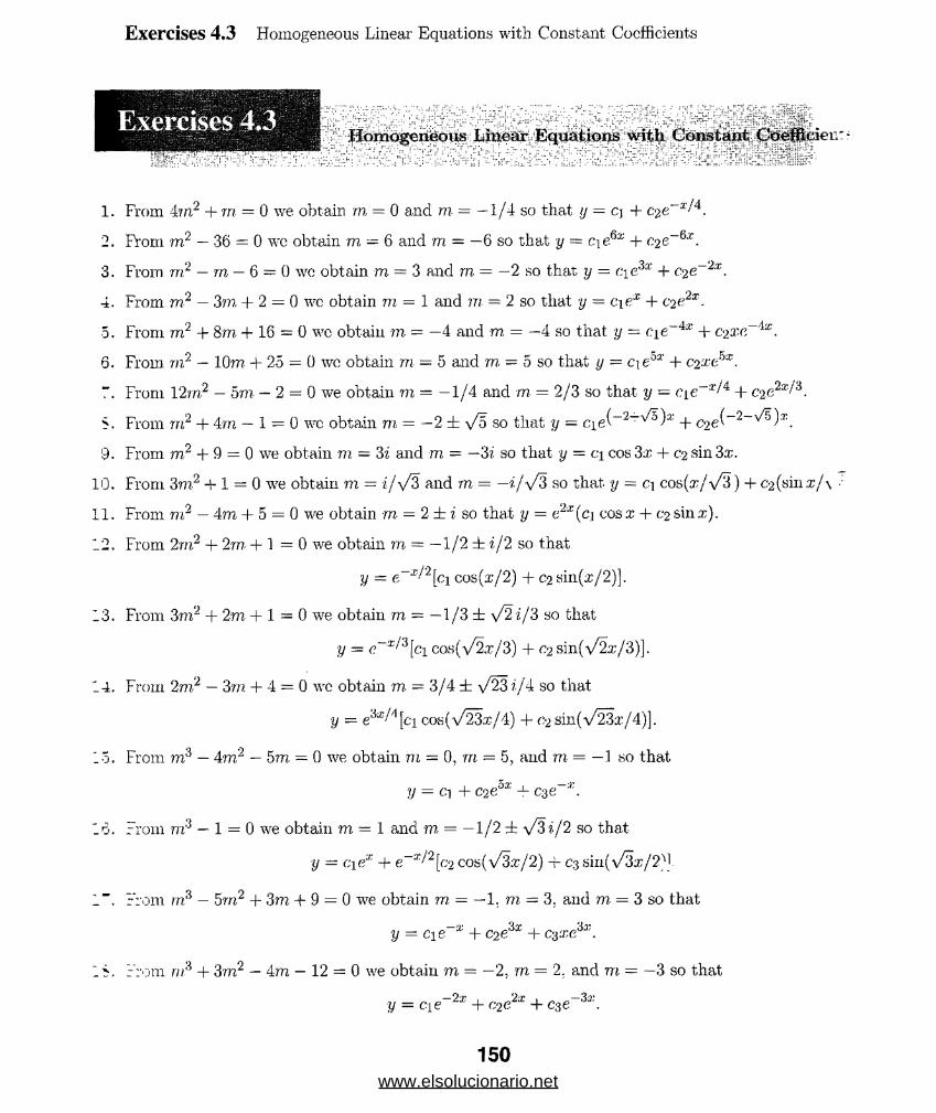
Exercises 4.3 Homogeneous Linear Equations with Constant Coefficients
Homogeneous Linear Equations with Constant CoefScieir ■
1. From 4rri2 + rn = 0 we obtain rn = 0 and rn = —1/4 so that y = cj + c^e"3'-4.
2. From m2 — 36 = 0 wc obtain m — 6 and m = — 6 so that y = c\ eQx + C2 e~&x.
3. From rn1 — rn — 6 = 0 we obtain m = 3 and rn = —2 so that y = cie3* + c.2 e~2x.
4. From rri2 — 3?n + 2 = 0 we obtain rn = 1 and rn = 2 so that y = ciex + C2 ?2x-
5. From m2 + 8m + 16 = 0 wc obtain m = —4 and m = —4 so that y = cie~‘lx + C2 xe~'lx.
6. From rn.? — 10m + 25 = 0 we obtain rn — 5 and rn -■ 5 so that y = c\eox + c^xe™.
From 12m2 — 5m — 2 = 0 we obtain m = —1/4 and m = 2/3 so that y — eie~x/4 +
S. From m2 + 4m — 1 = 0 wc obtain rn = —2 ± Vo so that y = cie(~2~^a}x + C2e(_2~v ) r.
9. From m2 + 9 = 0 we obtain m = 3i and m = —3? so that y = c\ cos 3:r + c,2 sin 3x.
10. From 3m2 + 1 = 0 we obtain m = if \/3 and m = —i/\/3 so that y = ci cos(x/\/3) + c-2 (sin xj \ ’■
11. From rn2 — 4m + 5 = 0 we obtain rn = 2 ± i so that y = e2x(cj cosx + C2sinx).
12. From 2m2 + 2rn +1 = 0 we obtain rn = —1/2 ± i/2 so that
y - e~x!'2[ci cos(x/2) + C2sin(x/2)].
13. From 3m2 + 2m +1 = 0 we obtain m = —1/3 ± y/2i/ 3 so that
y = cos(v/2,r/3) + c-2 sin(\/2a:/3)].
14. From 2m2 — 3m + 4 = 0 wc obtain m = 3/4 ± \/23 i/4 so that
y _ 009( /23.7;/4) 4- c:2 sin(\/23a:/4)].
1-5. From — 4m2 - 5m ■ 0 we obtain m = 0, rn = 5, and m = —.1 so that
y = ci + C2 eax + C3e_:';.
16. From m3 — 1 = 0 we obtain m = 1 and m = —1/2 ± y/Zi/2 so that
y = 6ie x + e~x/2[c2 cos(VSx/2) + 03 sin(v/3a;/2''l.
1". From m3 — 5m2 + 3m + 9 = 0 we obtain rn = — 1. m = 3. and m = 3 so that
y = c\e~x + C2 e'ix + Oixeix.
15. From m3 + 3m2 — 4m — 12 = 0 we obtain m = —2, m = 2, and rn = —3 so that
y = c-ie-2x + C2C2a: + cge-33’’.
150www.elsolucionario.net
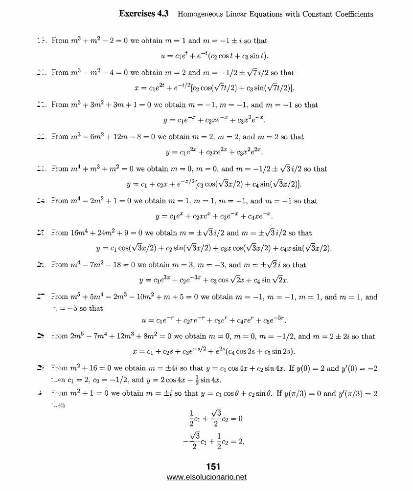
Exercises 4.3 Homogeneous Linear Equations with Constant Coefficients
From m3 + to2 — 2 = 0 we obtain rn = 1 and rn = — 1 ± i so that
u = Ci e* + e-* (c2 cos t + c% sin t).
From m3 — m2 — 4 = 0 we obtain m = 2 and m = —1/2 ± a/7 i/2 so that
x = c\e2t + e~^2[c2cos(V7t/2) + C3sin(\/7t/2)].
From to3 + 3m2 + 3m + 1 = 0 wc obtain to = —1, m = —1. a,nd m = — 1 so that
y = c\e~x + C2 xe~x + c3 X2e~x.
From to3 — (im2 + 12m — 8 = 0 we obtain m, = 2, rn = 2. and to = 2 so that
V = cic2x + C2.xe2'r + c’3.T2e2;r.
From m4 + m3 + to2 = 0 we obtain m - 0, m = 0. and m = —1/2 ± \[3i/2 so that
y = ci + C2X + e_3:'/2[c3 cos(\/3£-/2) + C4 sin(%/3a:/2)].
From m4 — 2m2 + 1 = 0 we obtain m = 1. to = 1. rn = —1, and rn = — 1 so that
y = ciex + C2 xe'r + c^e~x + c,\xe~x.
From 16m4 + 24m2 + 9 = 0 we obtain m = ±\/3?'/2 and m = ±\/3*/2 so that
y = ci cos(-'/3ir/2) + C2 sin(\/3:r/2) + C3X cos(V3a;/2) + 04.eesin(\/3ar/2).
From m4 — 7m? — 18 = 0 we obtain rn = 3, rn = — 3, and m = ±\/2 i so that
y = c\e?x + C2 e~ix + C3 cos y/2x + C4 sin \/2x.
From m° + om4 — 2m3 — 10m2 + m + 5 = 0 we obtain m = —1. m = —1, m — 1, and rn = 1, and
= — o so that
u — cie~r + c2re~r + cza’’ + C4 rer + C5e_or.
From 2m5 — 7m4 + 12m3 + 8m2 = 0 we obtain rn = 0, m = 0. m = —1/ 2, and m = 2 ± 2t so that
x = ci + C2 s + C3fi“ 's/2 + e2,s(c4 cos 2s + C5 sin 2s).
From to"2 + 16 = 0 we obtain m = ±4? so that y = c\ cos 4:r + C2 sin 4x. If y(0) = 2 and y;(0) = —2
■'-'.en ci = 2. C2 = —1/2. and y = 2cos4:c — \ sin4x.
From m2 + 1 = 0 we obtain rn = ±i so that y = c\ cos# + c-2 sin 0. If y(7r/3) = 0 and y\n/3) = 2
'I'-tU1 >/350. + T <* = 0
\/3 1-^-Ci + ~C2 = 2,
151www.elsolucionario.net

Exercises 4.3 Homogeneous Linear Equations with Constant Coefficients
so ci = —a/3; C‘2 = I, and y = —v/3 cos9 + sin#.
31. From m2 — 4m — 5 = 0 we obtain rn — —1 and m — 5, so that y = c:\e~1 + c.2 e5t. If y{ 1} =
and y\ 1) = 2, then cie-1 + C2e5 = 0, — cie-1 + 5c2e° = 2, so c\ = —e/3. C2 = e-5/3.
y = + ^e0*-0.
32. From 4m2 — 4m — 3 = 0 we obtain m — —1/2 and m = 3/2 so that y = cie-* '2 + C2e3x'/2. If ;t/(0 =
and y'(0) = 5 then a+ c -2 = 1. — |ci + |e2 — 5, so ci = —7/4. C2 — 11/4, and y = —je~x/2+^€ ’
33. From m2+m-1-2 = 0 we obtain m = —1/2±\/7if 2 so that y = e-x/2[ci C0s(\/7x/2)+C2 sin(\/7.r _
If y(0) = 0 and y;(0) = 0 then ci = 0 and 0 2 = 0 so that y = 0.
34. Prom nr — 2m + 1 = 0 we obtain m = 1 and rn — 1 so that y = ciex + c.2 xex. If y(0) = 5
y'{0) = 10 then c\ — 0, C\ + C2 = 10 so c\ = 5, 02 — 5, and y = 5ex + 5xea\
35. From m3+12rn2+36m = 0 we obtain m — 0, rn = —6, and m = —6 so that y - C[+C2e~6s;+C3.rfr“
If y(0) = 0. y'{0) = 1, and y"(0) = —7 then
ci + C2 = 0, — 6c*2 + C3 = 1. 36c2 — 12c‘3 — — 7.
so ci = 5/36; C2 = —5/36. C3 = 1/6. and y = — j^e-6a: + gxe_6:r.
36. From m3 -I- 2m2 — 5m - 6 = 0 we obtain rn = — 1, m = 2, and m = — 3 so that
y = cie_;c + C2 e2x + C3(5_3x.
If y(0) = 0, j/(0) = 0, and y"(0) = 1 then
Ci + C2 + C3 = 0, —Ci + 2c2 — 3C3 = 0, Cl + 4C2 + 9c3 = 1,
so C] = —1/6, C2 = 1/15. C3 = 1/10. and
y = -~e~x + — e2x + — e~3x. y 6 15 10
37. From m2 — 10m + 25 = 0 wc obtain m = 5 and m = 5 so that y — cicM + C2 xer>x. If y(0) ~ 1
y(l) = 0 then c\ = 1, cie° + C2e5 = 0, so ci = 1. C2 = — 1, and y = e5* — xe5x.
3S. From m2 + 4 = 0 we obtain rn = ±2i so that y = c\ cos 2x -F (>2 sin 2x. If y(0) = 0 and y(-K =
then ci = 0 and y — C2 sin 2x.
39. From m2 + 1 = 0 wc obtain in — ±i so that y = c\ cosx + (‘2 sinx and y' — — c\ 81113; -4- C2 c.
From y'(0) = ci(0) + 0*2(1) = C2 = 0 and t/(-w/2) = — ci(l) = 0 we find ci = C2 = 0. A solutk:
the boundary-value problem is y = 0.
40. From m2 — 2m + 2 = 0 we obtain m = 1 ± i so that y = ex(c.\ cosx + C2sinx). If y(0) = 1
i / :~ ) = 1 then ci = 1 and y ( i t ) = e * c m i r = —e1T. Since —en ^ 1, the boundary-value probloir.
110 solution.
152www.elsolucionario.net

Exercises 4.3 Homogeneous Linear Equations with Constant Coefficients
The auxiliary equation is rn2 — 3 = 0 which has roots —y/S and \/3. By (10) the general solution
is y = c i ^ + C2e-v3:c. By (11) the general solution is y — c ico shy ^ + C2Sinh\/3tf- For
y = c\e^x + the initial conditions imply ci + c% = 1. \/3ci — \/3('2 = 5. Solving for c-\ and
c-2 we find c\ — ^(1 -+5\/3) and c-j = |(1 — 5\/3) so y = ^(1 + 5v/3)ev ;r — ^(1 — oVS)e~'^x. For
y - ci cosh '/3x + c? sinh y/Sx the initial conditions imply c\ = 1. \fZc2 - 5. Solving for c\ and C2
we find ci = 1 and C2 == |V3 so y = cosh \/3x + |\/3sinh VSx.
The auxiliary equation is m2 — 1 = 0 which has roots —1 and 1. By (10) the general solution is
.;/ = ciex + C2 C~X■ By (11) the general solution is y = ci cosh x + C2 sinh x. For y = c,\ + oic-rx the
boundary conditions imply Ci + C2 — 1. cie — r^c" 1 = 0. Solving for c\ and C2 we find ci — 1/ (1+ e2)
and C‘2 = e2 /(1 + e2) so y = ex/(1 + e2) + e2e~x/(l + e2). For y = c\ cosh x + o>. sinhx the boundary
conditions imply ci = 1. C2 ‘ — tanh 1. so y ■ cosli x — (tanh 1) sinh x.
The auxiliary equation should have two positive roots, so that the solution has the form
y = ci&klX + coek-x. Thus, the differential equation is (f).
The auxiliary equation should have one positive and one negative root, so that the solution has the
form y = c\eklX + c-2 e~k2X. Thus, the differential equation is (a).
The auxiliary equation should have a pair of complex roots a±/3i where a < 0. so that the sohition
has the form eaa(ci cos 3x + c*2 sin,&t). Thus, the differential equation is (c).
The auxiliary equation should have a repeated negative root, so that the solution has the form
;j - C\e~x + C2 'xe~x. Thus, the differential equation is (c).
The differential equation should have the form y" + k2y = 0 where k = 1 so that the period of the
solution is 2tt. Thus, the differential equation is (d).
The differential equation should have the form y" + k‘2y - 0 where A; = 2 so that the period of the
solution is 7r. Thus, the differential equation is (b).
Since (m—4)(m+5)2 - m3+6m2- 15m—100 the differential equation is y/"+6y/f — 15yr — lOOy = 0.
The differential equation is not unique sincc any constant multiple of the left-hand side of the
differential equation would lead to the auxiliary roots.
A third root must be m3 = 3 — i and the auxiliary equation is
(rn + ^ [m - (3 + i)][m - (3 - i)} = (m + ^ (rn2 - 6;r + 10) = rn* - ~^rn2 + 7rn + 5.
The differential equation is
/ ' - y / + V + % = 0.
From the solution yi = e~ix cos x we conclude that mi = —4 + i and m2 = — 4 — i are roots of the
auxiliary equation. Hence another solution must be y2 = e-4xsin.r. Now dividing the polynomial
153www.elsolucionario.net
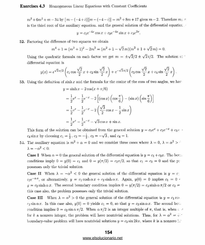
Exercises 4.3 Homogeneous Linear Equations with Constant Coefficients
1 r 1 , = - 5 «- -- 2
m3 + 6m2 -f m — 34 by [ m — (—4 + x)] [m - (—4 - •*')] = m2 + 8m + 17 gives m - 2. Therefore m? -~
is the third root of the auxiliary equation, and the general solution of the differential equation ■
y = cie-4x cos x -+ cae-4* sin x + c^e2*.
52. Factoring the difference of two squares we obtain
m4 + 1 = (rn2 + l)2 — 2 m2 — (m2 + 1 — \/2 m)(m2 + 1 + V2m) = 0.
Using the quadratic formula on each factor wc get m = ±\/2/2 ± \/2 i j 2 . The solution o:
differential equation is
/ \ \/2r/2 / . a/2 \ —v/2:r/2 / . y/2 \y(;r) = e', / I ci cos — a- + c-2 sin — x \ + e % I C3 cos x -r C4 sm — x 1 .
53. Using the definition of sinh x and the formula for the cosine of the sum of two angles, we liav
•y = sinh.x — 2 cos(x 4- tt/6)
(cosx) ^c o s^ — (sin a;) ^sin ^
1 r 1 _ r „ (V3 1 . \- -(•;■-- e — 2 cos x — - smx
2 2 \ 2 2 J 1 1
= -e'!: — -e~x — V3c(xsa; + sinx.2 2
This form of the solution can be obtained from the general solution y = c\ex + c^e~x + c$ c >
C4 sin x by choosing ci = 5 , c-2 = — £ ; c.3 — — \/3, and C4 = 1.
54. The auxiliary equation is m2 + a — 0 and we consider three cases where A = 0, A = or2 > •’
A = —a 2 < 0:
Case I When a = 0 the general solution of the differential equation is y = o\ + C2 X. The bor.:.
conditions imply 0 = y(0) = c\ and 0 = y(ir/2) = cxk/2 . so that ci = c-2 = 0 and the p:
possesses only the trivial solution.
Case I I When A = —a2 < 0 the general solution of the differential equation is y — c-
C2 e~Qx. or alternatively, y - c'i cosh ft x + <>2 sinh a. x. Again, y(0 ) = 0 implies ci = 0 *
y = ( ‘2 sinh ft x. The second boundary condition implies 0 = y(ir/2) = 0 2 sinh a tt/2 or c-2 =
this case also, the problem possesses only the trivial solution.
Case I I I When A = oi2 > 0 the general solution of the differential equation is y = c\ cor-
r -2 sinftx. In this case also, y(0) = 0 yields c\ — 0, so that y = 0 2 sin a- x. The second bov..
condition implies 0 = (>2 sin a tt/2. When an/2 is an integer multiple of 7r, that is. when --
for k a nonzero integer, the problem will have nontrivial solutions. Thus, for A = a2 = -• "
boundary-value problem will have nontrivial solutions y = C2sin2A;:/;. where k is a nonzero
154www.elsolucionario.net

Exercises 4.3 Homogeneous Linear Equations with Constant Coefficients
.:: the other hand, when « is not mi even integer, the boundary-value problem will have only the
• ::vial solution.
’."•ring a CAS to solve the auxiliary equation m3 — 6m2 + 2m + 1 we find m i = —0.270534,
": = 0.658675, and m3 = 5.61186. The general solution is
-0.270531:;: , „ J).658(i7S.x , „ Oo.61186xy = c\c + C-2 G + c$e
".'.'ing a CAS to solve the auxiliary equation 6.11m3 + 8.59m2 -I- 7.93m + 0.778 = 0 we find
■_ = —0.110241. m 2 = -0.647826 + 0.857532i, and m3 = -0.647826 - 0.8575321 The general
'; lut-ion is
y = Cie-0.110241X + e-0-647826ar(C2COsa857532a. + C3 sin 0.857532.7;).
’.’sing a CAS to solve the auxiliary equation 3.15m4 — 5.34m2 + 6.33m — 2.03 = 0 we find
.: = —1.74806. m2 = 0.501219, m3 = 0.62342 + 0.588965*, and m4 - 0.62342 - 0.588965't. The
..eneral solution is
y = cie-1-™06* + c2ea5012mr + e°-62342a?(c3 cos 0.588965® + c.i sin 0.588965,?;).
Vsing a. CAS to solve the auxiliary equation m4 + 2m2 — rn + 2 — 0 we find mi - 1/2 + \/3i/2.
-\2 = 1/2 — \/Z i/ 2 . m3 = —1/2 + -\/7i/2, and m.4 = —1/2 — y/li/2. The general solution is
, 1 2 ( Vs . v/3 \ _r/0( V7 . s/ 1 \y = e‘7 I ci cos — x + c2 sm — x I + e '" I C3 cos — x + C4 sm — a; 1 .
From 2m4 + 3m3 — 16m2 + 15m — 4 = 0 we obtain m = —4, rn = | . m — 1, and m = 1, so that
j = cie_4x + c2 ex ! 2 + c$ex + c,\xex. If y{0) = —2. y'{0) = 6, ^(O ) — 3, and y"'(0) = \ , then
Ci + C'2 + 03 = —2
—4 c i + — C2 + C3 + (’4 = 6
116cx + —C-2 + C3 + 2c4 = 3
-64ci + ^c2 + C3 + 3c4 = ^ ,
„ _ 4 _ _116 - _ 918 __ 58 „„ jsO Cl — 7Q . C2 — 3 ' ~ 25 ■ “ 5 > al1
4 _ ir 116 ,/ , 918 _ 58 „y = ~— e u -- 7r e + ~^rex --- xeJ\
Yb 3 25 5
From m4 — 3m3 + 3m2 — rn = 0 we obtain m = 0, m — 1. m = 1. and m = 1 so that
y = ci + C2 ex + C3 xex + C4 £ 2 e*. If y(0) = 0. y'(0) — 0. y"{0) = 1, and y'"(0) = 1 then
Cl + C2 = 0, C2 + C3 = 0, C2 + 2c3 + 2c4 = 1, C'2 + 3cg + 6C4 = 1,
155www.elsolucionario.net

Exercises 4.3 Homogeneous Linear Equations with Constant Coefficients
so ci = 2. c-2 — —2, c-3 = 2. c-4 — —1/ 2. and
y = 2- 2ex + 2xex - \xi€e.Z
Undetermined Coefficients — Superposition Approach
1. From rri2 + 3m + 2 = 0 we find mi = — 1 and m2 = —2. Then yc = cie-* + C2 e~2x and we assum.
yp = A. Substituting into the differential equation we obtain 2A = G. Then A = 3. yp = 3 and
y — cie x + C2C' ~'2* + 3.
2. From 4rri2 + 9 = 0 we find mi = — § i and m 2 — | i. Then yc = c\ cos |.t + C2 sin and we assnn:-.
yp = A. Substituting into the differential equation we obtain 9A = 15. Then A = | , yv = | and
3 . 3 5■y = ci cos -x + C‘2 sin -x + - .
Z t-t o
3. From rri2 — 10m + 25 = 0 we find mi = m2 = 5. Tlicn yc = + ojxe™ and we assun.
yp = Ax + .13. Substituting into the differential equation we obtain 25.4 = 30 and —10.4 + 25B = •:
Then A = | . B = i , yv = |x + § , and
y = cie " + C2 xe + -x + - .5 5
4. From m2 + rn — 6 = 0 we find m i = —3 and m2 = 2. Then yc — cie~'ix + C2 e2x and we assui:.
yp — Ax + B. Substituting into the differential equation we obtain —6.4 = 2 and A — 6B = 0. Th.
.4 = - § , B = , yp = ^ , and
—3 r 2 x ^ ^y = cie 'ix +c2e l - -x - — .
o. From ^m2 + m + 1 = 0 we find mi = m2 = —2. Then yc = C\ e~2x + c.2 xe~2x and wc assui:.
yp = Ax2 + Bx + C. Substituting into the differential equation we obtain A = 1, 2A + B = —.
and \A + B + C = 0. Then A = 1, B = —4, C = 5 . yp = x2 — 4x + | , and
y = cie~2x + C2 xe~2x + x2 — 4x + -.
6. From m2 — 8rn + 20 = 0 we find m i = 4 + 2i and m2 = 4 — 2i. Then yc = eix(ci cos 2x + C2 sin2.
and we assume yp = Ar2 + Bx + C + (Dx + £J)ex. Substituting into the differential equation r
156www.elsolucionario.net
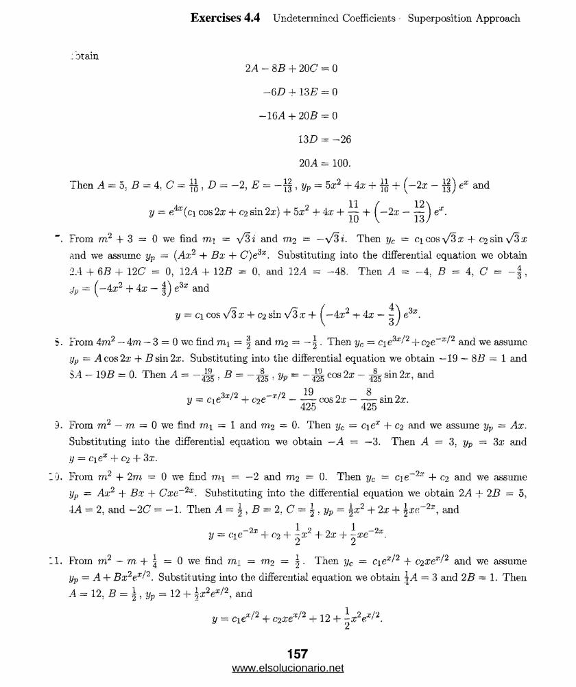
Exercises 4.4 Undetermined Coefficients - Superposition Approach
; otain2A - SB + 20C = 0
-6D + 1SE = 0
-16,4 + 20 B = 0
132? = -26
204 = 100.
Then A = 5; B = A. C = ^ , D = —2, E = — , yp = 5x2 + Ax + jjj -+ (—2x — ex and
y = e4x(c\ cos 2a: + eg sin2z) + 5a:2 + Ax + ^ 2x — ex.
From m2 + 3 = 0 we find m\ = y/3i and m2 = —a/3 i. Then yc = ci cos V3 + C2 sin \/3 .x
and we assume yp = (Ax2 + Bx + C)e3x. Substituting into the differential equation we obtain
2-4 + 6B + 12C = 0, 12A + 12B = 0, and 12A = -48. Then A = -A, B = 4, C = - § ,
:jp = (—4:r2 + 4x — e3x and
y = c\ cos \/3x + C'2 sin y/% x + 4.t2 -t- 4ar — ^ e?x.
5. From 4m2 — 4m — 3 = 0 wc find mi = 5 and m2 = — 5 . Then yc = c\eix’2 + C2e_a:/2 and we assume
ijp = A cos 2a; + Bsin 2x. Substituting into the differential equation we obtain —19 — 8B = 1 and
SA — 19£? = 0. Then A = — , B = — |g . yp = — cos 2x — |g sin 2rc, and
y = ^ie3x'/2 + c2e~x-2 - ^ cos 2« - — sin 2x.
9. From rn2 — m = 0 we find rn-i = 1 and m2 = 0. Then yc = c\ex + c2 and we assume yp = Ax.
Substituting into the differential equation we obtain —A = —3. Then A = 3. yp = 3x and
y = ciex + C2 + 3x.
-0. From m2 + 2rn - 0 we find m\ = —2 and m2 = 0. Then yc = ci e~2x + c2 and we assume
yp = Ax2 + jB.t + Cxe~2x. Substituting into the differential equation we obtain 2A + 2B = 5,
4A = 2, and — 2C = — 1. Then A = \ , B = 2, C = | = 5.T2 + 2x + ijxr;-2*, and
y = cie_2-T + c2 + + 2x + i;re_2a:.
.1. From m2 — rn + = 0 we find m i = m2 = 5 • Then yc = c\ex!2 -f o2xex-'2 and we assume
yp = A + Bx2ex'2. Substituting into the differential equation we obtain | A = 3 and 2B = 1. Then
A = 12, B = i , = 12 + \x2ex'2, and
y = c,\ex‘2 + C2 Xext2 + 12 + ^x2e^2.
157www.elsolucionario.net
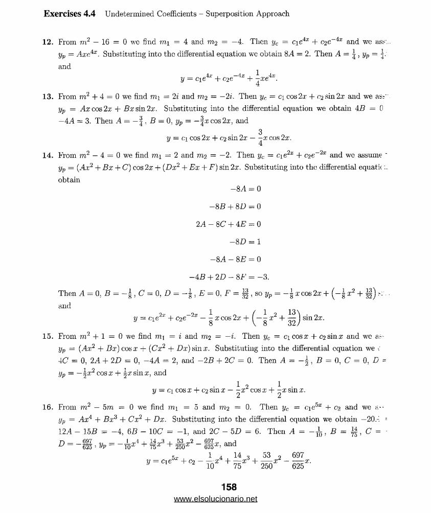
Exercises 4.4 Undetermined Coefficients - Superposition Approach
12. From rn2 — 16 = 0 wc find mi = 4 and m,:2 = —4. Then yc == c\e4x + o2e~4x and we ass...
yp - Axe4x. Substituting into the differential equation wc obtain 8.4 = 2. Then A = | , yp =
and
y = c\e4x + C2 (~4x + 7«e4;);.4
13. From m2 + 4 = 0 we find m\ = 2i and m 2 = —21 Then yc — c\ cos 2;r + <12 sin 2:r and we as?'
yp = Ax cos 2x + Bx sin 2x. Substituting into the differential equation we obtain 4B = 0
—4A = 3. Then .4 = — | , B = 0. yp = —\xc,os2x.: and3
y = ci cos 2x + ( ‘2 sin 2x — -x cos 2x.4
14. From m2 — 4 = 0 we find mi = 2 and m2 = —2. Then yc = c\e2x + C2 e~2x and wc assume '
y.p = (A t2 + Bx + C) cos 2x + (Dx2 + Ex + F) sin 2x. Substituting into the differential equa.ti(
obtain-8A = 0
-SB + 8D = 0
2A - 8C + 4E = 0
-8 D = 1
-8A -8E = Q
-4B + 2D - 8F = -3.
Then A = 0; B = — £ , C = 0, D = — | . E — 0, F = , so yp = a.-cos2;r + (—| x2 - I - •
and1 „ / 1 o 13'9 r —2r r\ ( l
y = c\e + C2 e - - x cos 2x + ( —- x -I- — I sm2x.
15. From rn2 + 1 = 0 we find mi = i and m2 — —i. Then yc = c\ cos x + c? sin x and wc a.--
ijp = (Ax2 + Bx) cosx -r (Cx2 -j- Dx) sinx . Substituting into the differential equation we •;
4C = 0, 2A + 2D = 0, -4A = 2, and -2B + 2C = 0. Then A = -5 , B = 0, C = 0, D =
Up = ~^%2 cos a; + Resins, and
1 9 1 .y — ci cos x + 0 2 sm x — ~x~ cos x + -x sin x.
16. From m2 — 5m - 0 we find mi = 5 and m2 = 0. Then yc = cie5x + c-2 and we a--
ijp = .4a:4 + BxA + Cx2 + Dx. Substituting into the differential equation we obtain -20.-' =
12.4 - 155 = -4, 6B - 10C = -1, and 2C - 5D = 6. Then A = - ± , B = i j £ ,C = ■D _ _697 _ _ J _ 4 , 14 .3 , 53. 2 _ 697 d ^ — 625 ’ yp — 10x ^ 75 ^ 250 6 2 5 ddm
5 . 1 a 14 y 53 2 69/V = c,e -+C2 - - X ■ + - * • + — *
158www.elsolucionario.net
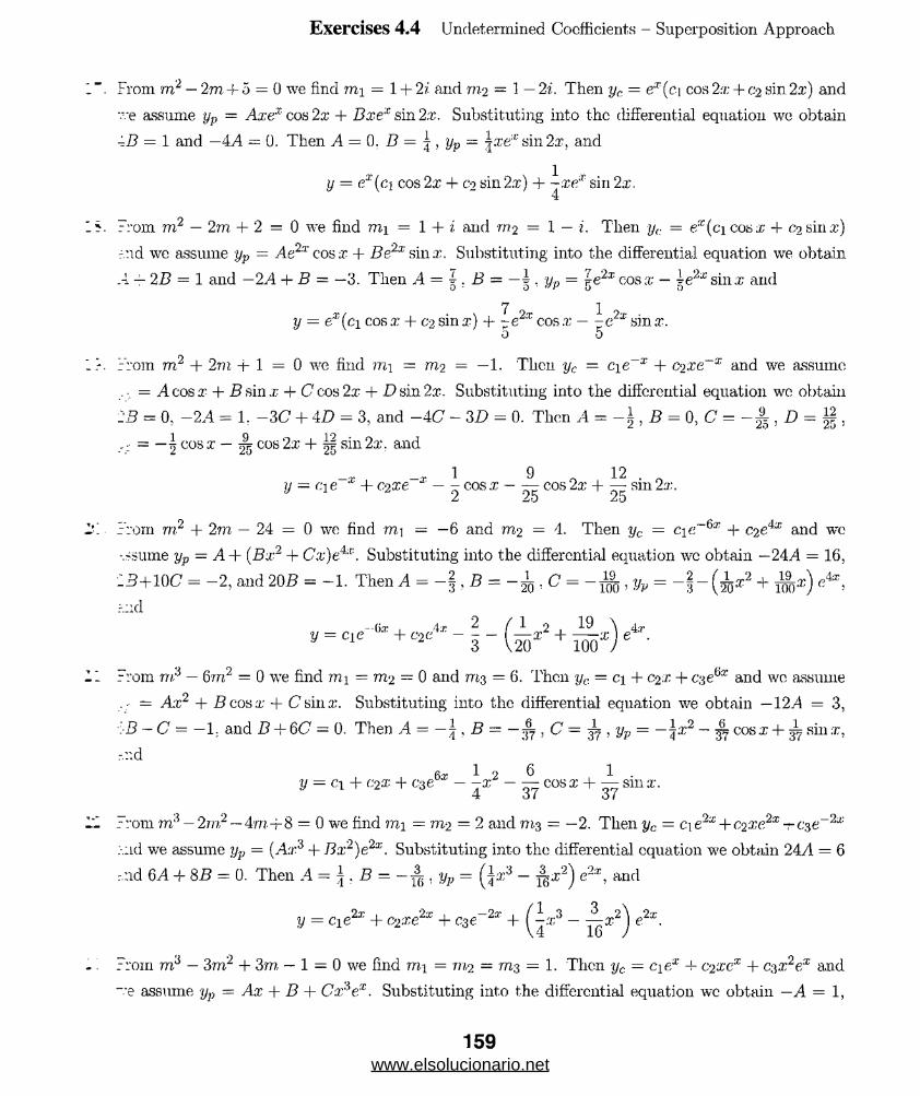
Exercises 4.4 Undetermined Coefficients - Superposition Approach
From rri2 — 2m + 5 = 0 we find m i = 1 + 2i and m-2 = 1—21 Then y(. = ex(ci cos 2x + 0 2 sin 2x) and
v.*e assume yp = Axex cos 2x + Bxex sin 2x. Substituting into the differential equation we obtain
-B = 1 and —4A = 0. Then A = 0. B = | , yp = |xe:,; sin2x, and
y = ex(ci cos 2x + co sin 2x) + sin 2x.4
From m2 — 2m + 2 = 0 we find mi = 1 + i and m 2 = 1 — i. Then y(. = e:c(cicosx + C2sinx)
r.nd we assume yp = -4e2'r cos x + Be2x sinx. Substituting into the differential equation we obtain
A — 2B = 1 and —2,4 + B = —3. Then A = ± . B = — i . y„ = ie2x cos x — ie2x sin x and0 ' O O OJ 1
y = ex(ci cos x + c-2 sin x) + ~e2x cos x — -c2x sin x.0 0
From m2 + 2 m + 1 = 0 we find m\ = m2 = —1. Then yc = c\e~x + C2xe~x and we assume
.• = A cosx + B sin x + C cos 2x + D sin 2x. Substituting into the differential equation we obtain
2B = 0, -2.4 = 1: -3C + 4D = 3, and —4C - 3D = 0. Then A = , B = 0, C = , D = § .
- = —5 cosx — ^ cos 2x + sin2x. and
-t 1 9 12 .y = c\ e + (>2 xe — - cos x — — cos 2x + —: sin 2x.
2 25 25
From rn2 + 2m — 24 = 0 we find m\ = —6 and m2 = 4. Then yc = cie~6x + C2e4x and we
-."Sume yp — A + (Bx2 + Cx)e4x. Substituting into the differential equation wc obtain —24.4 = 16,
1B+1QC = - 2, and 20B = -1. Then A = - ^ B = C = - ^ ,yp = Q }*2 + ^ x ) e4a\
y = * ,«- * + «</•' - | - ( I f + £ L X) e«
From m.3 — 6m2 = 0 we find mi = m2 — 0 and m3 = 6. Then yc = ci + c2x + and we assume
. = Ax2 + B cos x + C sin x. Substituting into the differential equation we obtain —124 = 3,
■IB - C = - 1. and B + 6(7 = 0. Then A = , B = — , C — ^ , yP = — Jx2 - ^ cosx + ^ sinx,
-nd6a- 1 2 6 1 .
V = Cl + c2x + c3e - - X - — cos x + — sm x.
From rn* — 2rn2 — 4m +8 = 0 we find m\ = m2 = 2 and m3 = —2. Then yc = Ci e2x + -rC3e_2a:
;-.:id we assume yp = (Ax3 + Bx2)e2x. Substituting into tlie differential equation we obtain 24A = 6
r.:id 6A + 8B = 0. Then A = \,B = - ^ , y p = (Jx3 - ^ x 2) elx, and
y = c.ie2x + C2 X(ilx + C3e_2a; + Q x 3 - e2x.
From m3 — 3m2 + 3m — 1 = 0 we find m-i = rn2 = m3 = 1. Then yc = ciex + C2 XCX + cyx2ex and
~’e assume yp = Ax + B + Cx*ex. Substituting into the differential equation wc obtain — A = 1,
159www.elsolucionario.net
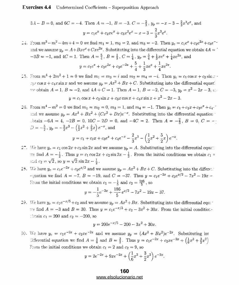
Exercises 4.4 Undetermined Coefficients - Superposition Approach
3.4 — B = 0. and 6(7 = —4. Then A = —1, B = —3, C - —| . yp = — x — 3 — ^x^e1, and
9y = ciex + C2.'rex + C3X2ex — x - 3 - - x3ex.
O
24. From m3-m 2 —4m+4 = 0 vve find mi = 1, m2 = 2. and m3 = —2. Then yc = c\ex+ c2e2x+c$e~'
and we assume yp = A+Bxex+Cxe2x. Substituting into the differential equation we obtain 4A = '
—■SB - - 1, and 4 C = 1. Then A = \, B = =\,yp = \ + ±;rex + \xe2x, and
y = c\?x + c2elx + cse~2x + 7 + \xex + ^xe2x.4 o 4
-5. From m '1 + 2m2 + 1 = 0 we find mi = m3 = i and m2 = m.4 = —i. Then yc = ci cos a? + C2sin; -
-V cos :r + C4X sin x and wc assume yp = Ak2 + Bx + <7. Substituting into the differential equat:
"v obtain A = 1. B = —2. and 4.,4 + (7 = 1. Then A = 1. B = —2, (7 = —3, yp = x2 — 2x — 3,
y = ci cos x + Co sin ;c + c^x cos x + c\x sin x + x2 — 2x — 3.
26. From m4 — m2 = 0 we find m i = m2 = 0. m3 = 1, and 7*14 = —1. Then yc = ci + C2« + 036* + C4-"
.Mid we assume = Ax6 + B.t2 + (Cfr2 + Dx)e~*. Substituting into the differential equation •
brain -6A = 4. -2B = 0, 10(7 - 2D = 0, and -4(7 = 2. Then A = - § , £ = 0. C =
^ » S/p = - §*3 - (s*2 + |*) «“*. and
x2 + e~x.
2~. We have yc = ci cos 2x + c2 sin 2.x and we assume yp = A. Substituting into the differential cquar.
v.t find A = — . Thus y = ci cos 2a: + C2 sin 2;k — ^ . From the initial conditions we obtain c\ -
c2 ~ V2. so y = y/2 sin 2x — .
25. We have yc = cje-2x + c2eX/'2 and we assume yp = Ac2 + Bx + C. Substituting into the differe:.'
-.;uation we find A = —7. B = —19, and C = —37. Thus y = c\e~2x + c2ex,!2 — 7x2 — 19a: —
From the initial conditions we obtain ci = — r} and c.2 = , so
1 _9a. 186 ,. /n _ 9 - „ _y/ : — -a -I— — e ' - 7a:" — 19rr — 37.
0 5
29. We have yc = ae~'x/5+C2 and we assume yp = Ax*+Bx. Substituting into the differential eqiu'
”'e find A = —3 and B = 30. Thus y = cie-r/0 + c.2 — 3x2 + 30a:. From the initial conditio:.-
:btain c\ = 200 and <;2 = —200, so
y = 200e_x/5 - 200 - 3a:2 + 30.x.
30. We have yc = c\e~2x + c2xe~2x and we assume yp = (A®3 + Bx2)e~2x. Substituting int
.arferential equation we find A = | and B = %• Thus y = c\e~2x + c2xe"2x + Q ®3 + |x‘2)
From the initial conditions we obtain c\ - 2 and c2 = 9, so
y = 2e_2a: + 9xe~2x + e~2x.
y = c\ + c2x + csex + C4 e x - :X' - -
160www.elsolucionario.net
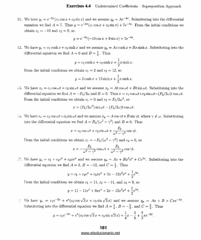
C‘-»
Exercises 4.4 Undetermined Coefficients - Superposition Approach
31. We have yc = e~2x(ci cos x + c2 sin ;r) and we assume yp = Ae~4x. Substituting into the differential
equation wc find A = 7. Thus ■;/ = e_2:!’(ci cos x + c-i sin x) + 7e~'ix. From the initial conditions we
obtain c± = —10 and C2 — 9. so
■y = e~2x(—lOcosa; + 9sin,r) + 7e~4x.
12. Wc have yc = c\ cosh x + c-2 sinh x and we assume yp = Ax cosh x + Bx sinh x. Substituting into the
differential equation we find A = 0 and B = \ . Thus
y = ci cosh x + c‘2 sinh x + ^x sinh x.
From the initial conditions we obtain ci = 2 and C2 = 12, so
1y = 2 cosh x + 12 sinh x + —x sinh a;.
z*
. We have xc — c\ cos u;t + 0 2 sin uit and we assume xv = At cos cot + Bt sin u>t. Substituting into the
differential equation wc find A = — Fq/2-uj and B = 0. Thus x = c\ cosutf+C2 sincjf—(Fo/2u)/ cos cot.
From the initial conditions we obtain ci = 0 and C2 = Fo/2ui2, so
x = (Fq/2u2) sinwt — (Fo/2uj)tcosujt.
:4. Wc have xc = ci cos u>t+C2 smart and we assume xp = A cos'yt+B&m'yt, where 7 ^ u). Substituting
into the differential equation we find A = Fo/(lo2 — 72) and B = 0. Thus
F0x = ci cos urt + c-2 sin cvt H— ---k cos71 .
U!‘i — 7Z
From the initial conditions we obtain ci = — Fo/(u>2 — 72) and c‘2 = 0, so
Fo Fox = -- ---r> cos u>t H— =---» cos 71 .
— 7 u>1 — 7^
:•!. Wc have yc: = c\ + c2ex + c$xex and wc assume yp = Ax + Bx2ex + Ceox. Substituting into the
differential equation we find A = 2, B = —12, and C = J?. Thus
1y = ci + c2ex + c‘sxex + 2x — I2x2ex + - e ox.
From the initial conditions we obtain ci = 11, c2 = —11, and C3 = 9, so
y = 11 - lie* + 9.Tex + 2x- 12x V + *e5a\
We have yc = cie 2x + ex(c2 cos \/3a: + C3 sin \/3x) and we assume yp = Ax + B + Cxe 2x.
Substituting into the differential equation we find A — | , B = — | , and C = | . Thus
www.elsolucionario.net

Exercises 4.4 Undetermined Coefficients Superposition Approach
From the initial conditions we obtain c\ = — . C2 = — . and 03 = . so
23 _ / 59 17 \ 1 5 2y
23 _9r 7’ ( 59 f— 1 I r~ . /— \ 1 O 2 — 2t = - — e + e‘ — jtt cosvix — — v3sm V 3x ) + -x - - -!- -xe .
12 V 24 (2 / 4 o o
37. We have yc = c\ C0SX — C2 sinx and wc assume yp = Ax? + Bx+C. Substituting into the differei:'
equation wc find A = 1. B = 0. and C = —1. Thus y = c.\ cosx + c-2 sinx + x2 — 1. From y(0) =
and y( 1) = 0 we obtain
ci -1 = 5
(cosl)ci + (sinl)c2 = 0.
Solving this system we find ci = 6 and C2 = — 6cot 1. The solution of the boundary-value pro!:'
is
y — 6 cos x — 6(cot 1) sin x + x2 — 1.
38. We have yc = ex(c\ cosx + C2 sinx) and we assume yp = Ax + B. Substituting into the differeiv
equation we find A — 1 and B = 0. Thus y = ex(ci cosX + C2 sinx) +x. From y(0) = 0 and y(tt; =
we obtain
ci = 0
tt — enci = 7r.
Solving this system we find ci = 0 and C2 is any real number. The solution of the boundary-v;.
problem is
y = C2 (::c sin x + x.
39. The general solution of the differential equation y" + 3y = 6x is y = ci cos a/3x + 02 sin\/3x — -
The condition y(0) — 0 implies c\ = 0 and so y = C2 sin \/3x + 2x. The condition ;t/(l) + y'( 1 -
implies c2 sin y/3 + 2 + C2\/3 cos \/3 + 2 = 0 so 0 2 = —4/(sin \/3 + VS cos \/?>). The solution is
—4 sin y/SxV — --- 7=— 7=--- 7= + 2x.
sin V3 + V3 cos V3
40. Using the general solution y — c\ cos \/3x+C2 sin y/3x+2x, the boundary conditions y(0)+j/(0 =
y(l) = 0 yield the system
c\ + a/302 + 2 = 0
c\ cos \/3 + (>2 sin V3 + 2 = 0.
Solving gives
2(—y/3 + sin\/3) , 2(1 —cos\/3)ci = —1=--- -j=-- ;— 7= ana 02 =
yf?i cos V3 — sin \/3 \/3 cos \/3 — sin \/3
162www.elsolucionario.net
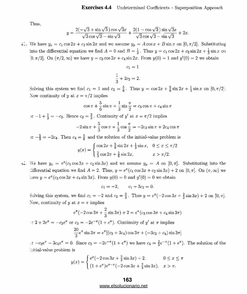
Exercises 4.4 Undetermined Coefficients - Superposition Approach
Thus,
2(—\/3 + sin \/3) cos \/3x 2(1 — cos V3) sin y/3xy — —----------- ------- -j- —-—------------- -— -j- 2x.
\/3 cos \/3 — sin \/3 \/3 cos \/3 — sin \/3
-41. We have yc = C; cos 2x + 02 sin 2x and wc assume yp = A cos x + D sinx on [0 . tt/2]. Substituting into the differential equation we find A = 0 and B = . Thus y = c\ cos 2x + C2 sin 2x + | sin x on 0. vr/2j. On (7t /2 , o o ) we have y = c% cos 2x + 04 sin 2x. From y(0) = 1 and y'(0) = 2 we obtain
ci = 1
i +2c2 = 2-
Solving this system wc find ci = 1 and C2 = g . Thus y = cos 2x + | sin2.r + | sin a; on [0, tt/2'.
Xow continuity of y at £ = tt/2 implies5 , 1 . 7T
cos 7r + - sm 7T + - sm — = C3 COS 7T + C4 sm 7T
:<r —1 + | = —C3. Hence C3 — | . Continuity of 1/ at x — 7t /2 implies5 1 7T .
—2 sm 7T + - cos 7T + - cos — = —2c3 sm tt + 2c4 cos o o ^
:>r — | = —2c4. Then C4 — | and the solution of the initial-value problem is( cos 2x + | sin 2x + | sin x, 0 < x < tt/2
y(x) = <[ | cos 2x + § sin 2x, x > tt/2 .■il. We have yc = ex(c\ cos 3a; + C2 sin 3x) and we assume yv = A 011 [0 , 7r], Substituting into the
differential equation we find A = 2. Thus, y = ex (ci cos 3a; + C2 sin 3a;) + 2 on [0,7r]. On (71% 00) we have y = ex(cz cos 3a; + c,\ sin 3a;). From y(0) = 0 and f/(0) = 0 wc obtain
ci - —2 , c\ + 3c2 = 0.Solving this system, we find ci = —2 and (>2 = § • Thus y - ex(—2 cos3a; -h § sin3x) + 2 on [0 , tt]. Xow, continuity of y at x = tt implies
2en (—2 cos 3tt + - sin 37r) + 2 = e" (as cos 3tt + C4 sin 3?r)
O
r 2 + 2(f — —036 or C3 = —2e_7r(l + eir). Continuity of 1/ at tt implies 20—e* sin 3% = e’r[(c3 + 3 4) cos 3ir + (—303 -h C4) sin 3tt]O
.r — C3e7r — 3c4e7r = 0. Since C3 = —2e~ff(l + e71-) we have C4 - | e _7r(l + e7r). The solution of the initial-value problem is
y(x) =ex(—2 cos 3a; + | sin 3z) 4- 2, 0 < x < 1r
(1 + e7r)e:K_"(—2 cos3a: + § sin3a;), x > tt.
163www.elsolucionario.net
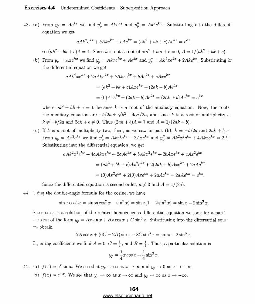
Exercises 4.4 Undetermined Coefficients - Superposition Approach
43. ' a) From yp = Aekx we find y'p = Akekx and yp = Ak2ekx. Substituting into the different:
equation we get
aAk2ekx + bAkekx + cAekx = (ak2 + bk -j- c)Aekx = ekx,
so (ak2 + bk + c)A = 1. Since k is not a root of am2 + brn + c = 0, A = 1 /(ak2 + bk + c).
i b) From yv = Axekx we find y'p — Akxekx 4- Aekx and yp : Ak2xekx + 2Akekx. Substituting i:.'
the differential equation we get
aAk2xekx + 2aAkekx + bAkxekx + bAekx + cAxekx
= (ak2 4- bk + c)Axekx + (2ak + b)Aeltx
= (0 )Axekx + (2 ak + b)Aekx = (2ak + b)Aekx = ekx
where ak2 + bk + c = 0 because k is a root of the auxiliary equation. Now, the root'
the auxiliary equation are —bf 2a ± Vb2 — 4ac /2a, and since k is a root of multiplicity
k 7 —bf 2a and 2ak + b ^ 0. Thus (2ak + b)A = 1 and A = I f (2ak + b).
Ic) If A" is a root of multiplicity two, then, as wc saw in part (b), k — —b/2a and 2ak + b =
From yp = Ax2ekx we find y'p = Akx2ekx + 2Axekx and y" = Ak2x2ekx + 4Akxekx — 2.4-
Substituting into the differential equation, we get
aAk2x2ekx + 4 aAkxekx + 2aAekx + bAkx2ekx + 2 bAxekx + cAx2ekx
= (ak2 + bk + c)Ax2ckx + 2(2 ak + b)Axekx + 2aAekx
= (0)Ax2ekx + 2(0 )Axekx + 2aAckx = 2 aAekx = ekx.
Since the differential equation is second order, a ^ 0 and A = l/ (2a).
44. Ysing the double-angle formula for the cosine, we have
sin x cos 2x = sin x(cos2 x — sin2 x) = sin a:(l — 2 sin2 re) — sin x — 2 sin3 x.
fr::.ce sin® is a solution of the related homogeneous differential equation we look for a part:
-' .utioii of the form yp = Ax sin x + Bxcosx -t- C sin'5 a;. Substituting into the differential equ? "
“■e obtain
2 A cos x + (6(7 — 2B) sin x — SC sin3 x = sin x — 2 sin3 x.
Equating coefficients we find .4 = 0, C = \ , and B = \. Thus, a particular solution is
1 1 . 3 yp = -x cos x + - sm x.
45. a) f ir ) — ex sin®. We see that yp —> oo as x —>■ oc and yp —>• 0 as x —» —oo.
■■ b ) f(x) = e~x. We see that yp ^ x as a: -> oo and yp —»• oo as x —> —oo.
164www.elsolucionario.net
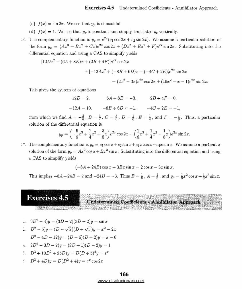
Exercises 4.5 Undetermined Coefficients - Annihilator Approach
(c) f(x) — sin2.x\ We see that yP is sinusoidal.
i'd) f(x ) = 1. Wro see that yp is constant and simply translates yc vertically.
The complementary function is yc = e2x(ci cos 2.x- + c-i sin2.r). Wre assume a particular solution of
:he form yp — (Aa:3 + Bx? 4- Cx)e2l: cos2 x + (Da:3 + Ex2 + F)e2x sin2 x. Substituting into the
differential equation and using a CAS to simplify yields
[1 2 Dx2 + (6A + 8 E)x + (2 B + A F))e2x cos 2x
+ [-12 Ax2 + (-8 B + 6 D)x + (-AC + 2 E)]eZx sin 2x
= (2a:2 — 3x)e2x cos 2x + (10a:2 — x — l)e2a; sin 2.x.
This gives the system of equations
121? = 2. 6A + BE = —3. 2 B + AF = 0.
—12 A = 10. —SB + QD = - 1, —AC t 2 E = - 1,
:rom which we find A = — , B = ^ , C = % , D = ^ , E = . and F = — | . Thus, a particular
-elution of the differential equation is
yp ■ ( —j.xA + 7X2 + |aAe2a’cos2a: + x3 + \x2 — e2xsin2 x.V o 4 8 / Vo 4 8 /
The complementary function is yc = ci cos x + 0 2 sin x+C3 X cos x+c.\x sin x. We assume a particular
solution of the form yp = Ax2 cos x + Bx* sin a;. Substituting into the differential equation and using
a CAS to simplify yields
(—8A + 2AB) cos x + 3 Bx sin x = 2 cos x — 3x sin x.
This implies —8A + 24S — 2 and —2 AB — —3, Thus B = | , A = | , and yp = ^x2 cos x -f |x3 sin x.
• * * ' ' '... . ' * - V-. ' Undetermined QgHefflcietits ^ \ [J
9D2 - A)y = [3D - 2) (3D + 2)y = sin a:
D2 — 5)y = (D — y/E)(D + y/5 )y = x2 — 2a:
D2 - AD - 12)y — (D - 6)(D + 2)y = x - 6
2D2 - 3 D - 2 )y = (2D + 1 )(D - 2 )y = 1
D3 + 10D 2 + 25 D)y = D(D + 5)2y = e*
D* + AD)y = D (D2 + A )y = rrr cos 2a:
165www.elsolucionario.net

Exercises 4.5 Undetermined Coefficients - Annihilator Approach
7. (D3 + 2D2 - 13D + 10)y = (D — 1)(D — 2)(D + 5)y = ze'®
8. (Da + 4D2 + 3D)y = D(D + 1)(D + 3)y = x2 cos a: — 3x
9. (D4 + 8D)y = D (D + 2)(D2 - 2D + 4)y = 4
10. (D4 - 8D 2 + 16)y = (D - 2)2(D + 2f y = (x3 - 2z)e4x
11. £>4?/ = D4(10x3 - 2x) = Da(30x2 - 2) = D2(60.x) = D(60) = 0
12. (2D - l)y = (2D - l)4ex/2 = 8DexI2 - 4ex/2 = 4exI2 - 4ex/2 = 0
13. (D-2)(D+5)(e2x+3e-5x) = (JD-2)(2e2x-15e-5l+5e2x+15e-5a:) = (D-2)7e2x = 14e2*-U- -
14. (D2 + 64) (2 cos 8x — 5 sin 8x) = £>(—16 sin 8a; — 40 cos 8a;) + 64(2 cos 8a: — 5 sin 8a:)
= —128 cos 8x 4- 320 sin 8;r + 128 cos 8a: — 320 sin 8x = 0
15. D 4 because of a;3 16. D:y because of x4
17. D(D — 2) because of 1 and e2x 18. D 2(D — 6)2 because of x and xe^x
19. D2 -i- 4 because of cos 2a: 20. D(D2 + 1) because of 1 and sin a;
21. D^(D2 + 16) because of a:2 and sin Ax
22. D 2(D2 + 1)(£>2 + 25) because of x, sin a:, and cos 5a;
23. (D + 1 )(D — l )3 because of e~x and x2ex
24. D(D — 1)(jD — 2) because of 1, ex, and e2x
25. D(D2 — 2D + 5) because of 1 and ex cos 2x
26. (D2 + 2D + 2)(D2 — 4D + 5) because of e~x sin x and e2x cos x
27. 1, x , x2, x3, x4
28. D2 + 4D = D(D + 4); 1, e~4x
29. e6x, e~Zx!2
30. D2 — 9D — 36 = (D — 12)(D + 3); e12x, e"3*
31. cos \/5 x, sin \/5 x
32. D2 - 6D + 10 = D 2 - 2(3)D + (32 + l 2); eax cosx, e3x sinx
33. D3 - 10D 2 + 25D = D(D - 5)2; 1, e5*, xe5x
34. 1. x, e5x, e7x
35. Applying D to the differential equation we obtain
D(D2 - 9)y = 0.
166www.elsolucionario.net

Then
Exercises 4.5 Undetermined Coefficients - Annihilator Approach
lj = cie3x + C2C 3x + C‘3
Vc
and yp = A. Substituting yp into the differential equation yields —9A — 54 or A = —6. The general
solution is
y = cie'ix t C2 e~Sx — 6.
:t. Applying D to the differential equation we obtain
D(2D2 -7D + 5)y = 0.
Then
y = c ie 0* /2 + C2ex + C3
Vc
and yp = A. Substituting yp into the differential equation yields 5.4 = —29 or A = —29/5. The
general solution is
y = c\eoxZ2 + c<2 ex — — .5
I". Applying D to the differential equation we obtain
D(D2 + D)y = D2(D + 1 )y = 0.
Then
y = C j + C2C X + C3.X'
Vcr.nd yp = Ax. Substituting yp into the differential equation yields A = 3. The general solution is
y = ci + C2 e~ix + 3a;.
. Applying D to the differential equation we obtain
D(D3 + 2D2 + D)y = D2(D + 1 )2y = 0.
Then
y = Cl + + C[]X(~x + C4 Xv - -.................-v ■ ■ - —........ v
yc
-nd yp = Ax. Substituting yp into the differential equation yields A = 10. The general solution is
y = ci + c2e~x + C‘ixe~x + 10ar.
- Applying D2 to the differential equation we obtain
D2(D2 + W + 4 )y = D2(D + 2 )2y = 0.
167
29
www.elsolucionario.net
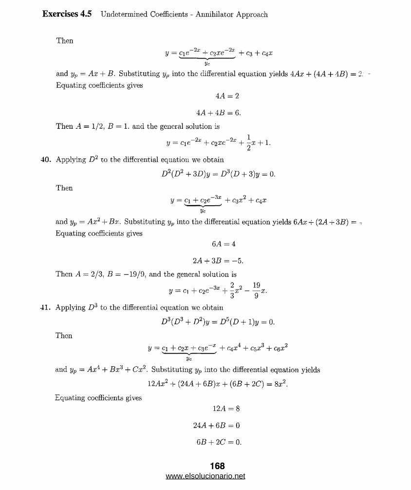
Exercises 4.5 Undetermined Coefficients - Annihilator Approach
Then
y = -4- C 2 xe ~ 2a + C3 + c ± xv V
yc
and y-p = Ax + B. Substituting yp into the differential equation yields AAx + (4/4 + 4B) = 2, -
Equating coefficients gives
AA — 2
AA + AB = 6.
Then A = 1/2. Z? = 1. and the general solution is
y = c i e _2a ' + C 2 xe ~ 2x + + 1.
40. Applying D 2 to the differential equation we obtain
D 2 {D2 + 3 D)y = DS(D + 3 )y = 0.
Then— ’V r 9
y = ci + C2e “ ' + c3x + C4 X'--- v----/
yc
and yp = Ax'2 + Bx. Substituting yv into the differential equation yields 6Ax -f (2A 4- 3B) = -
Equating coefficients gives
6A = 4
2A + 3B = -5.
Then A = 2/3, B — —19/9. and the general solution is
—3x 2 ^y = ci + C2C + 3^ -
41. Applying D3 to the differential equation we obtain
D 3 (D 3 + D2)y = £>5(£> + l)y = 0.
Then
y = ci + C2Z -r C3e~J + C4 X4 + Cr,x3 + c&x2 yc
and yp = Ax1 + Bx3 + Cx2. Substituting yp into the differential equation yields
12 Ax2 + [2AA + 6B)x + (6£ + 2 C) = 8z2.
Equating coefficients gives
12A = 8
24 A + 6B = 0
6B + 2C = 0.
168www.elsolucionario.net
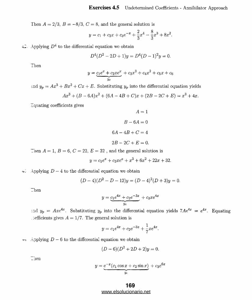
Exercises 4.5 Undetermined Coefficients - Annihilator Approach
Then A — 2/3, B = —8/3, C = 8, and the general solution is
—t 2 a 8 o oy = ci + C2& + cge + -x - -ar + 8x .
t j
Applying D4 to the differential equation wc obtain
D\D2 -2D + 1 )y = D i (D - 1 f y = 0.
Then
y = ciea: + C2 xex + C3X3 -h c^x2 + c$x + cq'----V----'
yc
r.,ixd ijp — Ax? + Bx2 + Cx + E. Substituting yv into the differential equation yields
Ax3 + (B — 6A)x2 + (6A — 4B + C)x + (2 B — 2C + E) = x3 + 4x.
Equating coefficients gives
4 = 1
B - 6A = 0
6A-4B + C = 4
2B -2C + E = 0.
Then A = 1, B = 6. C = 22, ,E = 32 . and the general solution is
y = c\ex + C2 xez + x3 + 6x2 4- 22x + 32.
Applying D — 4 to the differential equation we obtain
(D — 4)(D2 - D — 12 )y = (D - 4 f (D + 3 )y = 0.
Then
y = cie4i: + c^e-3* + c$xe4x'---- v—---'
Vc
>.nd ijp = Axe4*. Substituting yp into the differential equation yields 7Ae4x = e41.
. j efficients gives A = 1/7. The general solution is
y = cie4x + C2 e~'ix + ^xe4x.
Applying D — 6 to the differential equation we obtain
(D — 6)(D2 + 2D + 2)y = 0.
Then
y = e~x(ci cosx + 0 2 sinx) + c- e v ^
Vc
169
Equating
www.elsolucionario.net

and yp = Aebx. Substituting yp into the differential equation yields 5(Me6a: = 5e&x. Ecr.
coefficients gives A = 1/10. The general solution is
y = e~x(c\ cos x 4- c-2 sin x) +
45. Applying D(D — 1) to the differential equation we obtain
D(D - 1)(£>2 - 2 D - 3 )y = D(D - 1 )(D + 1 )(D - 3 )y = 0.
Then
y = C\e*x + oie~x + C3 ex + c.4s v y
Vc
and yp = Aex + B. Substituting y.p into the differential equation yields —4Aex — 3B = 4-
Equating coefficients gives A = — 1 and B = 3. The general solution is
y = cie3x + c2e~x - ex 4- 3.
46. Applying D2(D + 2) to the differential equation we obtain
D 2(D + 2 )(D2 + 6D + 8)y = D2(D + 2 f{D + 4 )y = 0.
Then_,9'r zL-'t* _9/ti
y = c\e + c-2 e •' + c$xe + c^x + eg
yc
and yp = Axe~2x + Bx + C. Substituting yp into the differential equation yields
2Ae “x + SBx + (6B + 8C7) = 3e 2x + 2x.
Equating coefficients gives
2A = 3
SB = 2
6B + SC = 0.
Then A = 3/2, B = 1/4, C = —3/16 , and the general solution is
y = <v-2* + c2e-41 + Ive-2* + \x -2 4 16
47. Applying D2 + 1 to the differential equation we obtain
(D2 + 1 )(D2 + 25 )y = 0.
Then
y = ci cos 5x + C2 sin 5x + C3 cos x -+ C4 sin x
yc
Exercises 4.5 Undetermined Coefficients - Annihilator Approach
170www.elsolucionario.net
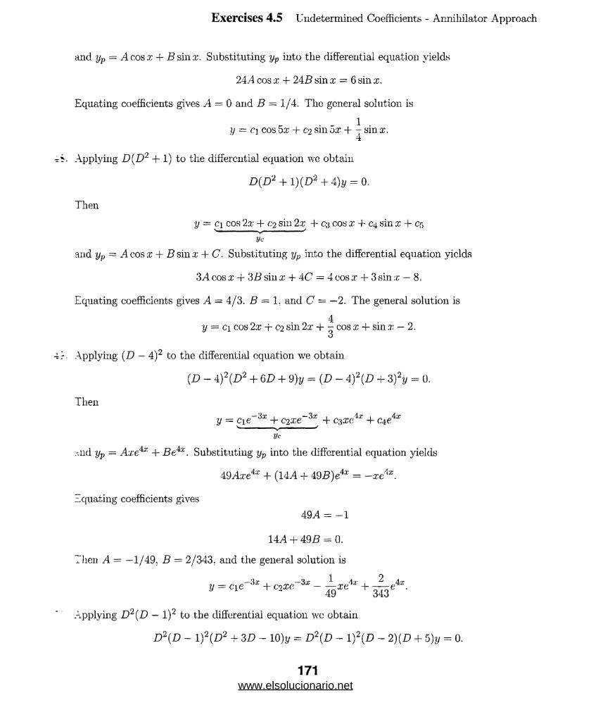
Exercises 4.5 Undetermined Coefficients - Annihilator Approach
and yp = A cos x + B sin x. Substituting yv into the differential equation yields
24/1 cos x + 24 B sin x = 6 sin x.
Equating coefficients gives A = 0 and B — 1/4. The general solution is
1 .y = ci cos ox + C2 sin ox + - sin x.
Applying D(D2 + 1) to the differential equation wc obtain
D(D ‘2 + l)(D'2 + 4)y = 0.
Then
y = c\ cos 2x + o>. sin 2x + c» cos x + c% sin x + cr>'------ V------ '
yc
and yv = A cos x + B sin x + C. Substituting yp into the differential equation yields
3 A cos x + 3B sin x + 4C = 4 cos x + 3 sin x — 8.
Equating coefficients gives A = 4/3. B = 1. and C ~ —2. The general solution is
4y - ci cos 2x + c-2 sin 2x + - cos x + sin x — 2.
o
Applying (D — 4)2 to the differential equation we obtain
(D - 4 f ( D 2 + 6D + 9)y = (D - 4 f (D + 3 f y = 0.
Then
y - cie~'ix + C2 xe~3x + c^xeix 4- c±eAx v „ ✓Vc
-nd yp - Are4* + Beix. Substituting yp into the differential equation yields
49 Axe4* + (14A + 49 B)e4x = -zeix.
Equating coefficients gives
49A = -1
14A + 495 = 0.
Then A = —1/49, B = 2/343. and the general solution is
y = c i e " 3;K + c 2x c ~ 3x - + ^ e 4:K.
Applying D2(D — I )2 to the differential equation wc obtain
D2(D - 1 f(D~ +3D - 10)1/ = D2(D - 1 f{D - 2){D + 5)y = 0.
171www.elsolucionario.net
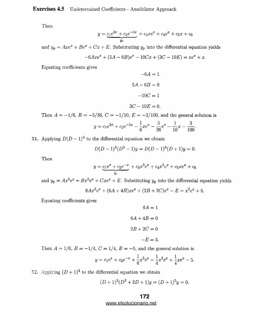
Exercises 4.5 Undetermined Coefficients - Annihilator Approach
Then
= C[62X + C26 0X + C;yX,eX + C±eX + C$X + CQyc
and ijp — Axe£ + Bex + Cx + E. Substituting yp into the differential equation yields
-6Axex + (5A - 6B)ex - 10Cx + (3C - 10£ ) = xex + x.
Equating coefficients gives
-6A = 1
5A — 6B = 0
- 10C = 1
3 C - 10£ = 0.
Then A = —1/6, B = —5/36, C = —1/10. E — —3/100. and the general solution is
y - c\^x + C2 e~ x -- xex — — e* — —x -- — .y 6 36 10 100
51. Applying D(D — I )3 to the differential equation we obtain
D(D - 1 f{ D 2 - 1)|/ = D(D - 1 )4(£> + 1 )y = 0.
Then
y — c\ex + C2 e~x + C3 X'iex + C4 X2ax + c^xex + ce'----V----'
y<:
and yp = Ax3ex + Bx2ex + Cxex + E. Substituting yp into the differential equation yields
GAx2ex + (6A + 4B)xex + (2J3 + 2C)e:c ~ E = x2ex + 5.
Equating coefficients gives
6A = 1
6A + AB = 0
2B + 2C = 0
- E = 5.Then A — 1/6. B = —1/4, C = 1/4, E = —5, and the general solution is
y = c±ex -f C2 e~x + ~x3ex — \x2ex + \xex — 5.6 4 4
52, Applying {D + l )3 to the differential equation we obtain
(D + 1 )3(D2 + 2D + 1 )y = (D + 1 f y = 0.
172www.elsolucionario.net

Exercises 4.5 Undetermined Coefficients - Annihilator Approach
Then
y — c\e x + C2 xe x + c;ix4e x + c ^ e x + c$x2e x
yc
and yp = Ax4e~x + Bx:ie~x + Cx2e~x. Substituting yp into the differential equation yields
12Ax2e~x + 6Bxe~x + 2Ce~x - x2e~x.
Equating coefficients gives A = B = 0. and C = 0. The general sohition is
y = c\erx + C2 xe~x + ~-x4e~x.JL Z
Applying D2 — 2D + 2 to the differential equation wc obtain
(D2 -2D + 2)(D2 - 2D + 5)y = 0.
Then
y = ex (ci cos 2x + C2 sin 2x) + ex(c cos x + C4 sin x)'--------v--------'
yc
r. ud yv = Aex cosx + Bex sinx. Substituting yp into the differential equation yields
3 Aex cos x + 3 Bex sin x = ex sin x.
Equating coefficients gives A = 0 and B = 1/3. The general solution is
1y = ex(a cos 2x + 02 sin 2x) + ~e3, sin x.
o
Applying D2 — 2D + 10 to the differential equation we obtain
(D2 -2D + 10) (d 2 + D + £ ) y = (D2 - 2D + 10) ( d + - J y = 0.
'lien
y — c\e x-2 + C2 xe 'T//2 + czex cos 3x + C4 ex sin 3x
yc
■-.ad yp = Aex cos3x + Bex sin3x. Substituting yp into the differential equation yields
(9B — 21A/A)ex cos 3x — (9.4 + 27B/A)ex sin 3x = —ex cos 3x + ex sin 3x.
Equating coefficients gives27
-~~A + 9B = -14
27- 9 A - — B = 1.
4
Then A = —4/225, B ~ —28/225. and the general solution is
-,/9 4 , „ 28 rr
www.elsolucionario.net

Exercises 4.5 Undetermined Coefficients - Annihilator Approach
55. Applying D 2 + 25 to the differential equation we obtain
(D2 + 2b) (D2 + 25) = (D2 + 25)2 = 0.
Then
y = a cos oar + co sin 5.t + C3 X cos 5.x + C4 X cos 5x s : '
Vc
and yp = Ax cos bx + Bx sin ox. Substituting yp into the differential equation yields
10 B cos bx — 10 A sin 5a’ = 20 sin ox.
Equating coefficients gives A = — 2 and B = 0. The general solution is
y — ci cos 5x + C2 sin 5x — 2x cos bx.
56. Applying D2 + 1 to the differential equation we obtain
(.D2 + 1)(£>2 + 1) = (D2 + l )2 = 0.
Then
y — ci cos x + C2 sin x + c$x cos x + C4 X cos x
Vc
and yp = Ax cosx + Z?xsinx. Substituting yp into the differential equation yields
2 B cos x — 2 A sin x — 4 cos x — sin x.
Equating coefficients gives A = 1/2 and B — 2. The general solution is
y — ci cos x + C2 sin x + \x cos x — 2x sin x.z
57. Applying (D2 + l )2 to the differential equation we obtain
{D2 + 1)2(D2 + D + 1) = 0.
Then
3/ = e x/2 V3 ^ . Vzd cos — x + C2 sin — x + C3 cos x + Ci1 sin x + c$x cos x + c q x sin x
Vc
and yp — A cos x + B sin x + Cx cos x + Ex sin x. Substituting yp into the differential equatio:.
(B + C + 2E) cos x + Ex cos x + (—A — 2C + E) sin x — Cx sin x = x sin x.
Equating coefficients gives
B + C + 2E = Q
E = 0
- A - 2 C + E = 0
- C = 1.
174www.elsolucionario.net
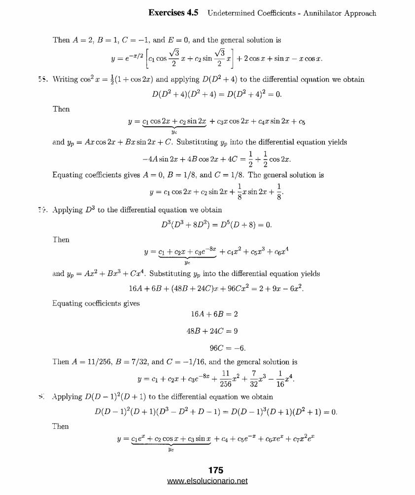
Exercises 4.5 Undetermined Coefficients - Annihilator Approach.
Then A = 2, D = 1, C = —L and E = 0, and the general solution is
y = e - x /2 V3ci cos — x + Co sm —— x
2 22 cos x + sin x — x cos x.
5 S. Writing cos2 a; = |(1 + cos 2 x) and applying D(D 2 + 4) to the differential equation we obtain
Then
D(D2 + 4)(D2 + 4) - D(D2 + 4)2 = 0.
y = ci cos 2 x + C‘2 sin 2 x + c%x cos 2 x + C4 X sin 2 x + 0 5
V<:
and yp — Ax cos 2 x + Bx sin 2 x + C. Substituting yp into the differential equation yields
1 1—4A sin 2x + 4B cos 2 x + AC = - + - cos 2 x.
Equating coefficients gives A = 0 . B — 1/8. and C = 1/8. The general solution is
1 1y = ci cos 2 x + c‘2 sin 2 x + -x sin 2 x + -.
8 8
Applying D3 to the differential equation we obtain
£>3(D3 + 8 D2) = D5(D + 8) = 0.
Then
y — c\ + C2 X + cze~8x + c,\x2 + c$xs + c^x4s------------------ v ------------------ /
yr.
and yp = Ax2 + Bx:3 + Cx4. Substituting yp into the differential equation yields
16A + 6 B + (A&B + 24(7):/: + 96Cx2 = 2 + 9x- 6 x2.
Equating coefficients gives
ISA + 6 B = 2
ASB + 2AC = 9
96 C = -6.
Then A = 11/256, B = 7/32, and C = —1/16, and the general solution is
y = ci + c2x + c3e Sx + — x‘ + — x° - — x*.2o6 32 16
Applying D(D — I ) 2 (D + 1 ) to the differential equation we obtain
D{D - 1 f{D + 1)(D3 - D 2 + D - 1) = D(D - 1 f ( D + 1 ){D2 + 1) = 0.
11 7 „3 1 .4
i hen
y = cie* + C2 cos x + C3 sin x + C4 + c&e x + cqxex + c^x^e
yc
175www.elsolucionario.net
and yv = A + Be~x + Cxex + Ex2 ex. Substituting yp into the differential equation yields
4Exex + (2C + 4E)ex - 4Be~x — A = xex - e~x + 7.
Equating coefficients gives
4E = 1
2C + 4E = 0
-4 B = -1
-A = 7.
Then A = —7. B = 1/4, C = —1/2, and E = 1/4. and the general solution is
y = c\ex + C2 cos a; + C3 sin a: — 7 + -e~x — -xex + \x2ex.4 2 4
61. Applying D 2(D — 1) to the differential equation we obtain
D\D - 1 )(D3 - 3D2 + 3D - 1) = D2(D - l )4 = 0.
Then
y = ciex + C2 xex + czx2 ex + C4 + c$x + cqx^c*
yc
and yp = A + Bx + C'x*ex. Substituting yp into the differential equation yields
{-A + 3B) -B x + 6 Cev = 16 - x + e*.
Equating coefficients gives
-A + 3 B = 16
—B = -1
6 C = 1.
Then A — —13, B — 1 . and C = 1/6, and the general solution is
y = c\ex + C2 xex + c-iX?ex - 13 + x + \xAex. 6
62. Writing (ex + e~x)2 = 2 + e2x + e~2x and applying D(D — 2)(D + 2) to the differential equa:
obtain
D(D - 2)(D + 2)(2D3 - 3D2 - 3D + 2) = D(D - 2)2(D + 2)(D + 1)(2D - 1) = 0.
Then
y - ci< ~:r + C2 <?x + czex ! 2 + 0 4 + c$xe2x + c<;e~2*
Vc
Exercises 4.5 Undetermined Coefficients - Annihilator Approach
176www.elsolucionario.net

Exercises 4.5 Undetermined Coefficients - Annihilator Approach
and ijp - A + Bxe?x -j- Ca 2x. Substituting yp into the differential equation yields
2A + 9.Be2* - 20Ce-2;f = 2 + e2* + e-2*.
Equating coefficients gives A ~ B — 1/9. and C = —1/20. The general solution is
y = Clerx + c2e2x + c3e 2 + 1 + ^ e 2* - ±-e~2x.y 20
Applying D(D — 1) to the differential equation we obtain
D{D - 1 )(£>4 - 2DS + D 2) = D 3{D - l )3 = 0.
Then
y — ci + C‘ix + c.zex + C4xe* + c~,x2 + c§x2exS " ■ "Nr ■' "I y
Vc
and yp = Ax'2 + Bx2ex. Substituting yp into the differential equation yields 2A + 2Bex = 1 + ea
Equating coefficients gives A = 1/2 and B = 1/2. The general solution is
y = ci + c-2 a: + c$ex + C4 Xex + ^a;2 + ^x2ex.& &
Applying D?>(D — 2) to the differential equation we obtain
D3(D - 2)(£>4 - 4D2) = D 5(D - 2)2{D + 2) = 0.
Then
V = ci + c-2 X + cge2* + a e '2* + c$x2 -+- C6»3 + ojx4, + cgxe2*'-------- --------- '
Vc
and yp = Ax2 + Bx3 + Cx4 + Exe2x. Substituting yp into the differential equation yields
(—8*4 + 24(7) - 24Bx - 48Cx2 + 16£e2x = 5a:2 - e2a;.
Equating coefficients gives
-8A + 24C = 0
-245 = 0
-48C = 5
16 7 = - 1.
Then A = —5/16, B = 0, C = —5/48. and E = —1/16, and the general solution is
www.elsolucionario.net
Exercises 4.5 Undetermined Coefficients - Annihilator Approach
65. The complementary function is yc — c\eSx + &x. Using D to annihilate 16 we find yp =
Substituting yp into the differential equation we obtain —64A = 16. Thus A — —1/4 and
y = cxeSx + c2e-8x - J
8x o . 8a;
The initial conditions imply
Thus ci = C2 = 5/8 and
y' = 8cie — 8c2e .
5C l+ C 2 = -
8ci - 8c2 — 0.
5 5 _g2. 1
» - i ^ + 8e I '
66. The complementary function is yc = c\ + C2 (‘~x. Using D 2 to annihilate x we find yp — Ax - -
Substituting yp into the differential equation we obtain (A + 2B) + 2Bx — x. Thus A = - -
B = 1/2. and
—r 1 2y = ci + c2e " - x + -xZi
y1 = —C2 e~x — 1 + x.
The initial conditions imply
ci + c2 = 1
-C-2 = 1.
Thus ci = 2 and c2 = —1, and
1 2y = 2 — e — ir + - x .Zi
67. The complementary function is yc — ci+c2eox. Using D2 to annihilate x — 2 we find yp = Ax - -
Substituting yp into the differential equation we obtain (—5A+2S )—lOSx = —2+x. Thus A =
and B — —1/10, and
Kr 9 1 o y = Cl + C,e- + - X - - X
y' = 502^ + £ - k
The initial conditions imply
25 5
ci + c2 = 0
41
C 2 = 125
178www.elsolucionario.net

Exercises 4.5 Undetermined Coefficients - Annihilator Approach
Thus ci = —41/125 and C2 = 41/125, and
41 41 =T 9 1 o
y = -Jro + m e' " + 25x -Toz'-
The complementary function is yc = c\ex + C2 C~()X. Using D — 2 to annihilate 10e2x we find
yp = Ae2x. Substituting yp into the differential equation we obtain 8Ae2x = 10e2x. Thus A = 5/4
and
y = ci ex + C2 e~6x + ^e2as
y' = aex - 6c2e~6x + ~e2x.
The initial conditions imply
Cl + C2 = -\
r 3Cl - 6 C 2 - - - .
Thus ci = —3/7 and C2 = 5/28, and
y = —~ex + — e~6x + -e2ic y 7 28 4
• The complementary function is yc = c\ cos x + C2sinx. Using (D2 + 1 )(D2 + 4) to annihilate
8 cos 2x — 4 sin x we find yp = Ax cos x + Bx sin x + C cos 2x + E sin 2x. Substituting yp into the
differential equation we obtain 2B cos x — 3C cos 2x — 2A sin x — 3E sin 2x = 8 cos 2x — 4 sin x. Thus
.4 = 2, B = 0, C = —8/3, and E = 0, and
g
y = c\ cos x + c'2 sin x + 2x cos x — - cos 2xO
16y' = — ci sin x + C2 cos x + 2 cos x — 2x sin x -|- — sin 2x.
o
The initial conditions imply
8
C 2 + 3 = _1
—Cl — 7T = 0.
Thus Ci = —tt and 0 2 = —11/3, and
11 • ^ 8 y = —7r cos x — -sina: + 2x cos x — - cos 2x.O O
The complementary function is yc = Ci + c2ex + czxex. Using D(D — l )2 to annihilate xex + 5
we find yp = Ax + Bx2ex + CxAex. Substituting yp into the differential equation we obtain
179www.elsolucionario.net
Exercises 4.5 Undetermined Coefficients - Anniliilator Approach
A 4- (2B + 6C)eT + QCxex = xe:r + 5. Thus A — b ,B = -1/2, and C = l / 6; and
y = ci + C2ea; + C3>i'e'r + 5.x — ^.r2e:r 4- ^.r’3ex
y' = 026* + c$(xex + ex) + 5 — xex +
y" = c.2 ex 4- cz(xex 4- 2ex) — ex — xe* 4- ^x2 4- ^x3e*.
The initial conditions imply
Cl + C2 = 2
C2 + C3 + 5 = 2 C2 + 2cg — 1 = —1.
Thus ci = 8, C2 = —6. and C3 = 3, and
y = 8 — Qex + 3xe;t’ + ox — ]-x2ex + ^x3ex.2 6
"1. The complementary function is yc = e2x(ci cos 2x + C2sin2x). Using Z?4 to annihilate ..
find yp = A + Bx 4- Cx2 + Ex3. Substituting yp into the differential equation we t
i 8.4 - AB + 2C) 4- (SB - 8C + 6£)x 4- (8C - 12E)x2 + 8Ex3 = x3. Thus A = 0, B =
C = 3/16, and E = 1/8, and
3 3 1 y = e2x(ci cos 2x 4- C2 sin2x) 4- — x 4- — x2 + -x3
62, lb o
3 3 3y’ = e2x [ci (2 cos 2x — 2 sin 2x) 4- C2 (2 cos 2x 4- 2 sin 2x)] + ™ -r £ 4- x■x2.
32 8 8
The initial conditions imply
ci = 2
2ci 4- 2c2 4- ~ = 4.
Thus ci = 2, C2 = —3/64. and
2t/« « 3 . „ , 3 3 2 1-1 y = e/-l (2 cos 2x - — sm2x) 4- — x + — x2 + -x3.
’2. Tiie complementary function is yc = ci 4- c^x 4- C3X2 4- C4ex. Using D2(D — 1) to anni'
— ex we find yp = A x a + Bx4 + Cxex. Substituting yp into the differential equation we ■
180www.elsolucionario.net
Exercises 4.5 Undetermined Coefficients - Annihilator Approach
—6A + 245) — 24Dx + C'ex = x + ex. Thus A - —1/6, D = —1/24, and C = 1, and
y — C1 + C2 X + C3 X2 + c4(f - ~x3 - J-x4 + xex0 z 4
y' = c-2 -f 2C3X + aiex - ^a;2 - ^a?3 + ex + xex
y" = 2 C3 + C4ex — :c — ^x2 + 2 ex + xex.£
y'» = cAex -\ -x + 3e;c + are*
The initial conditions imply
ci + — 0
C2 + C4 + 1 = 0
2-C3 + C4 -j- 2 = 0
2 + 04 = 0.
Thus c 1 = 2, C2 = 1, c3 = 0, and c.4 — —2, and
y = 2 + x - 2 ex - lx 3 - x4 + xex.6 24
To see in this case that the factors of L do not commute consider the operators (xD — l)(D + 4)
-.r.d (D + 4)(xD — 1). Applying the operators to the function x we find
(xD - 1 )(D + A)x = (xD2 + AxD - D - 4)x
— xD2x + 4 xDx — Dx — Ax
= x(0) + 4x(l) — 1 — Ax — —1
-.ad
(D + A)(xD — l)a: = (D + 4)(arDa: — x)
= (D + 4) (x - l~ x) = 0.
7:;us, the operators arc not the same.
181www.elsolucionario.net
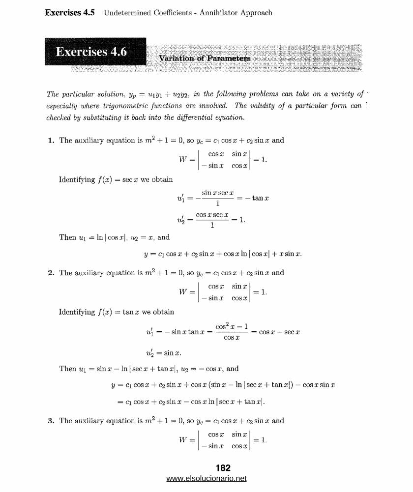
Exercises 4.5 Undetermined Coefficients - Anniliilator Approach
Variation of Parameters
The particular solution. yp — u\y\ + u-2 y-2 - in the following problems can take on a variety of
especially where trigonometric functions are involved. The validity of a particular form can
checked by substituting it back into the differential equation.
1. The auxiliary equation is m? + 1 = 0, so yc = ci cos x + c2 sin a: and
cos x sin xW =
sm a; cos x= 1.
Identifying fix) = sec a; we obtain
u\sm x sec x
1
cos x sec xUo
1
= — tan x
= 1.
Then uj = In | cosx|. U2 = x, and
y = c\ cos x + C2 sinx + cosx In | cosx| + x sin x.
2. The auxiliary equation is m2 + 1 = 0, so yc = c\ cos x + c2 sinx and
W =cos x sm x
— sin x cos x= 1.
Identifying f(x) = tanx we obtain
u[ = — sin x tan x =cos" x — 1
cosx= cos x — sec x
u2 = sin x.
Then ui = sin x — In | sec x + tan x|, u2 = — cos x, and
y = ci cos x + C2 sin x + cos x (sin x — In | sec x + tan x|) — cos x sin x
= ci cos x + C2 sin x — cos x In | sec x + tan x|.
3. The auxiliary equation is m2 + 1 = 0, so yc = c\ cos x + c2 sinx and
W =cos x sm x
-sinx cosx- 1.
182www.elsolucionario.net
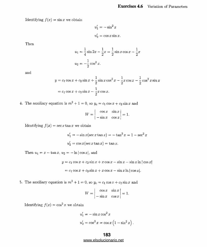
Exercises 4.6 Variation of Parameters
Identifying f(x) = sinx we obtain
u'i - — sin2 x
u2 = cos x s in x.
Then
l . r t l 1 . 1u\ — - sm 2x — -x - - sinx cosx-- x
4 2 2 2
1"U2 = — - cos x.
z
and
1 • 2 1 1 2y = ci cos x -f C2 sin x + - sm x cos x — -x cos x — - cos x sin x
= Cl COS X -r C2 sm x — —x cos x .£
4. The auxiliary equation is rn.2 + 1 = 0; so yc = C] cos x -f c-2 sin x and
cos x sm x
— sin x cos x: 1.
Identifying f (x )= sec x tan x we obtain
« i - — sin x(sec x tan x) = — tan2 x = 1 — sec2 x
«2 = cosx(secxtanx) = tan x.
Then ui = x — tanx. u2 = — In | cosx), and
y = ci cos x + C2 sin x + x cos x — sin x — sin x In | cos x|
- ci cos x + C3 sin x + x cos x — sin x In I cos x|.
•5. The auxiliary equation is m +1 = 0, so yc — ci cosx + c2 sinx and
cos x sin xW =
— sm x cos x= 1.
Identifying f(x) = cos2 x we obtain
u'i = — sin x cos2 x
u2r2 = co s3 X — COS X ( l — s i l l2 x ) .
183www.elsolucionario.net

Exercises 4.6 Variation of Parameters
Then u\ = | cos3 x, «2 — sin x — | sinJ x, and
y = ci cos x + C2 sin x + ^ cos4 x + sin2 x — ^ sin4 x0 o
= ci cos x + c-2 sin x + ^ (cos2 x + sin2 .xj (cos2 x — sin2 xj + sin2
1 9 ^ • 2 = ci cos x + c2 sm x + - cos" x + - sin x
0 o
1 1 • 2= ci cos x + C2 sm x + - + - sm x.o o
6. The auxiliary equation is m2 + 1 — 0. so yc = ci cos x + c2 sin x and
cos x sin x
X
W =— sm x cos x
= 1.
Identifying f(x) = sec2 x we obtain
u[sinx
cos2 x
Then
u2 = sccx.
1U i = = — sec x
cosx
u2 = In I secx + tan x\
andy = ci cos x + C2 sin x — cos x sec x + sin x In | sec x + tan x|
= ci cos x + C2 sin x — 1 + sin x In | sec x + tan x|.
7. The auxiliary equation is m2 — 1 = 0, so yc = ciex' + C2 ?~x and
W =ex e~x
ex —e x= -2.
Identifying f(x) = coshx = |(e x + ex) we obtain
www.elsolucionario.net
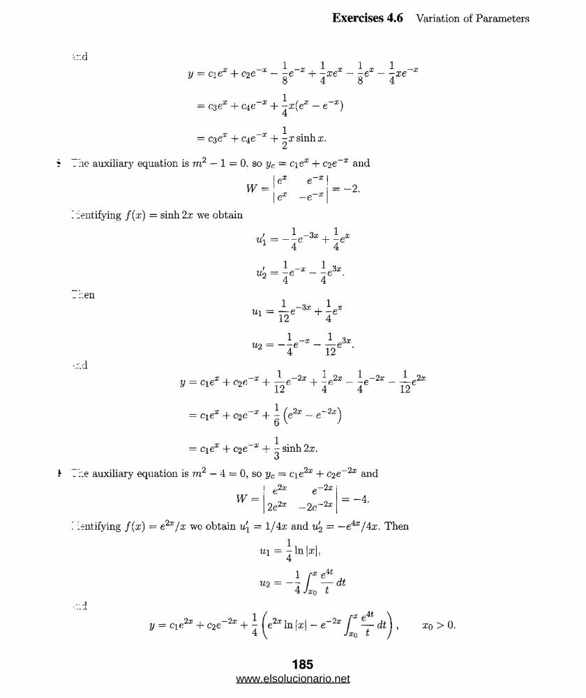
Exercises 4.6 Variation of Parameters
-.::d
y = Clex + c2e~x - ^e~x + ^xex - ^ex - ^xe~s
= c3ex + c4e~x + \x(ex - e~x)4
1= c$ex + c±e x + -a? sinhx.
£
The auxiliary equation is to2 — 1 = 0. so yc = c,\ex + C2 e~x and
I e* e~x !W = I = - 2.
ex —e x
identifying f(x) = sinh2.r we obtain
_ r.en
1: — T<
,-3* + * *4 4
1= -e * - -e3a\4 4
1 -3s + I x
12 4
1--- P -x 1 J3<x
4 12
-.r.d
y = cie* + e*r* + i e -21 + ^ ^ - ~e
= c1ex + c2e-x + U e 2x-e-21)
= ciex + c2e~x + ^ sinh 2a;.O
i 7;-.e auxiliary equation is m2 — 4 = 0, so yc - c\e2x + C2 e~2x and
W =! e2x e~2x
= -4.2e2x —2e 2x
’ iriitifying f(x) = e2x/x wc obtain u[ = l/4x and u'2 = —eAx/4x. Then
•u\ — J In |ar|.
1 fx e , u2 = - - / — dt4 J X(j t
y = c\e?x + c.2 e~2x + \ (e2x In |x| — e~2x f4 y Jx,
- d tXQ t )
,2x
XQ > 0.
185www.elsolucionario.net

Exercises 4.6 Variation of Parameters
10. The auxiliary equation is m2 —9 = 0. so yc = c\e6x -+ c2e 6X and
w = \ e'ix e 3ar= - 6 .
13e3x -Se~3x
Identifying f(x) = 9x/e3x we obtain u[ = ^xe_(ix and Then
1 -e* 1xe
and
Ul = “ 2i e
3 2“ 2 =
V = c1(> + C2 e - 31 - - ? A “ 3*24 4 4
1= cie3* + cse-te - ^ ^ ( l - 3®).
11. The auxiliary equation is m,2 + 3m + 2 = (m + l)(m + 2) = 0, so yc = c\e~x + c.2 e~2x and
„ —x 2x !
w =—e x —2e 2x j
i = —e -3x
Identifying f(x) = 1/(1 + e*) we obtain
cx«! =
■u2 —
l + ex
2xer
1 4- ex 1 + ex
Then u\ = ln(l + ex), u2 — ln(l + ex) — ex, and
ex.
y = Cle~x + c2e~ + e-* ln(l 4- ex) + ln(l + ex) - e~x
= C3e_x + c2e~2x 4- (1 4- e~x)e~x ln(l 4- e31).
12. The auxiliary equation is to2 — 2m + 1 = (m — l )2 = 0, so yc = c\ex + c2xex and
W =
Identifying f(x) = ex/ ( l + x2) we obtain
ex xex
ex xex 4- ex= e2x
ui =xexex
e2x (1 + x2) 1 4- x2
u2 ■exex 1
e2x( l+ x 2) 1 + x2'
186www.elsolucionario.net
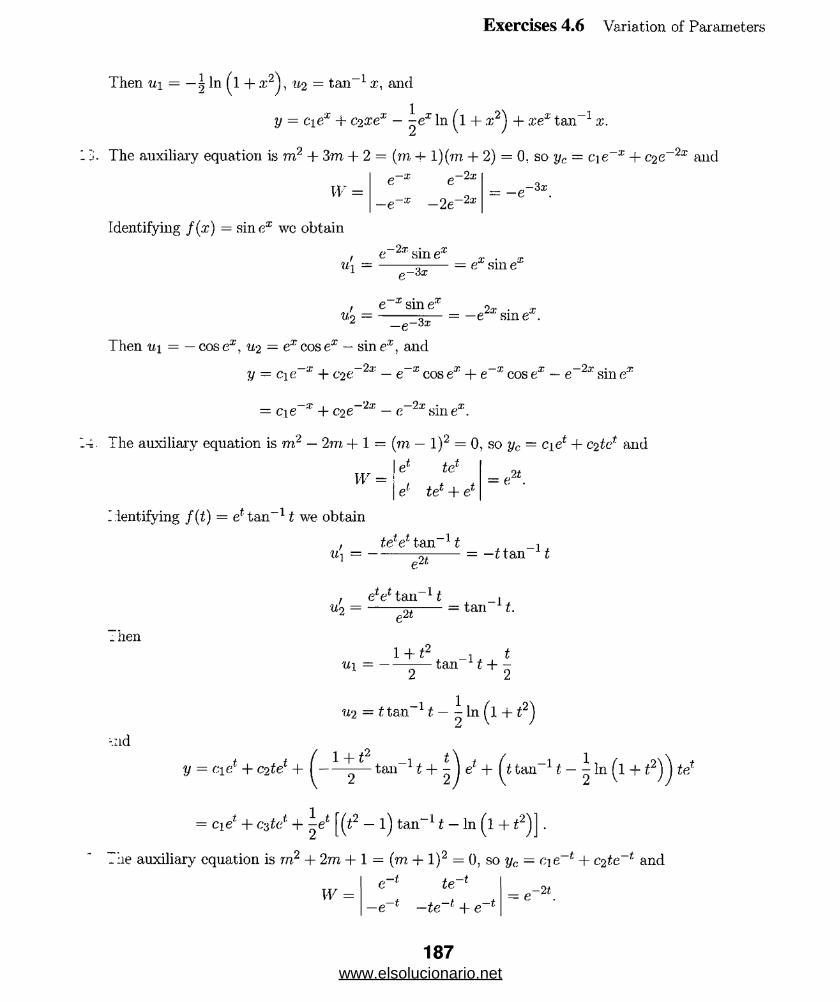
Exercises 4.6 Variation of Parameters
Then u\ = —-5 In ( l + x2j , u.2 = tan 1 x, and
y = ciex + C2 xex — ^ ex In ( l + :r2j + xex tan-1 x.
II. The auxiliary equation is m2 + 3m + 2 = (to 4- l)(m + 2) = 0. so yc = c\e~x + c2e~2x and2x
w =
Identifying f(x) = sin ex we obtain
—e
e x e
x -2e~2x—e—3x
, e 2x sin ex .* 1 = „ - 3 x = e a l I l e
v!2e x sin ex
_p 3x = —e2x sin ex.
Then u\ = — cose35, u2 = excosex — sinex, and
y — c\e x + c2e 2x — e x cosex + e x cos ex — e 2x sinex
= c\e x + C2e 2x — e 2x sin ex.
The auxiliary equation is m2 — 2in + 1 = (rn — l )2 = 0, so yc ~ cie* + c2tet and
1 j tetW=\
j el te1 + ef’= e21
lientifying f(t) = ef tan 11 we obtain
«i =ieV tan 1t
e21 — —t tan t
u2 =tan 1112T = tan t.
_ lien
u\ 1 + t' * -1 * * — tan t+ -
U2 = t tan-11 — - In ( l + 12)
-.nd
y = c\e + c2te +1 + t
2 tan t+-\e'
= cief' + cstc* -I- ^e* j £2 — l j tan 11 — In ( l + i2)] .
The auxiliary equation is rn2 + 2m + 1 = (to + l )2 = 0. so yc — c\ + C2 te~t and
?._t te~lW = = e— 2t
187www.elsolucionario.net
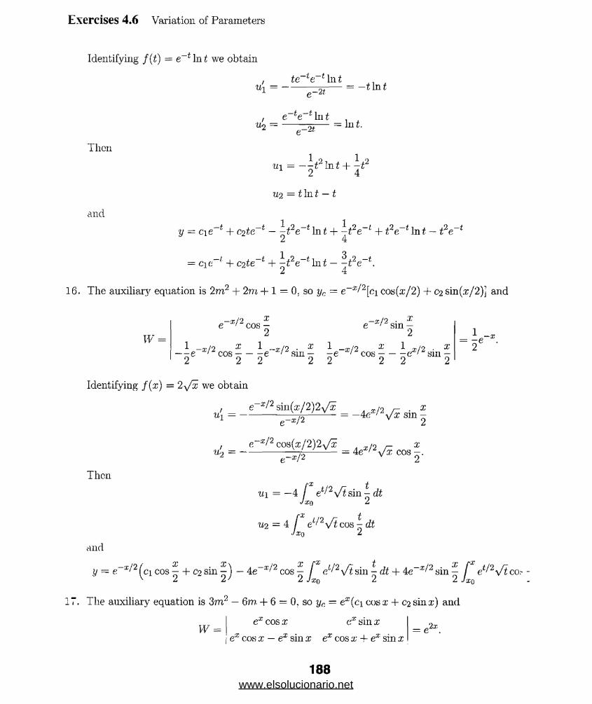
Exercises 4.6 Variation of Parameters
Identifying /(i) = e In t we obtain
te te *lni <>-2t —tin t
Then
and
, e te t hit .Kg = e_2i = h lt
1 2, 1 5u\ = — -t In i + -i
U2 = t In t — t
1 1y = cie_i + c^te-1 — - i2e_:t In i + -i2e~L + i2e_* In i — i2e_t
2 4
= cia~l + C2te~t + In i — ^ i2e_<.2 4
16. The auxiliary equation is 2m2 + 2m + 1 = 0, so yc = e x/2[c\ cos(x/2) + c2 sin(x/2)j and
W =
e x/2 cos — 2 e ^ 2sin
1 —r l 9 X’ 1 — -r/9 . X 1 — -r/9 X' 1 W 9 • X'—-e '" cos - — -e ' - sm - -e *C/ cos - — -a ' sin -2 2 2 2 2 2 2 2
26
Identifying f(x) = 2^/x we obtain
= _ e- ^ s iu ( x / 2)2y £ = /2 £
1 e_x/2 2
, e x/2 cos(x/2)21/x «2 = ---
X*
Then
ui = —4 I e*'12\ft sin t/LL‘0 2
/■X , £U2 = 4 / et/2^ cos - d
'Atq 2
di
and
y = e x'/2(ci cos + C2 sin — 4e :r/2 cos j sin dt + 4e x/2sin^ f et/2\/ico?v 2 27 2 7xo 2 2 ja?o
17. The auxiliary equation is 3m2 — 6m. + 6 = 0, so yr. — ex(ci cosx + C2sinx) and
W =ex cos x ex sin x
j ex cos x — ex sin x ex cos x + ex sin x= e2x
188www.elsolucionario.net

Exercises 4.6 Variation of Parameters
Identifying f(x) = |exsecx we obtain
, (ex sin x) (ex sec x) /3 1
« i = ------------- — = ' 3 tan*
, _ (ex cos x) (ex sec x) j 3 _ 1u2 - - 3 •
Then u\ = iln(cosx). U2 = lx , and
1 , 1y = C\ex cosx + C2ex sinx + - ln(cos x)ex cosx + -xex sin x.
3 3
W = = ex.
IS. The auxiliary equation is 4m2 — 4m + 1 = (2m — l )2 = 0. so yc = c\ex/2 + C2 xex/2 and
ex /2 x e x /2
l ex /2 L x e x /2 + eX /2
Identifying f(x) = jex/2V l — x2 we obtain
xex/2ex/2 /i ~ x2 1«! =
u2 =
Aexex/2 ex!2 \/l — x2 1
x2
46®
To find i6i and «2 we use the substitution u - l —x2 and the trig substitution x = sin (9, respectively:
« i
1 2 — -r \/l — a;2 + ^ sin 1 x.“2 = 8 V- " ' 8
Thus
y = cie*/2 ■+• C2 xex' 2 + - -e'r/2 ( l — x2) 3/* + \x2eXf2\j\ - x2 + \xex'2sin 1 x.12 ' o 8
1 f. The auxiliary equation is 4m2 — 1 = (2rn — l)(2m + 1) = 0, so yc = c\exl2 + C2C-X/2 and
VT =,3/2 -,—x/2
I x (2 _ l p - x f 2 i 2 2fc
= - 1.
Identifying /(x) = xex/2/A we obtain = x/4 and '<4 = —xex/A. Then ui = x2/8 and
2 = ~xex/A + ex/4. Thus
1/
-aid
= c\ex + coe x + \x2eX' 2 ~ \xex!2 + - e x/28 4 4
= C3,ex''2 + C2 (:~X/2 + \x2er' 2 — \xex' 28 4
if = \csexf2 - \c2e x/2 + px2ex/2 + ~xax2 - ~ex2. 2 2 lo o 4
189www.elsolucionario.net

Exercises 4.6 Variation of Parameters
The initial conditions imply
Tims C3 = 3/4 and c2 = 1/4, and
3 wo 1y - -ex!2 + ® / 2 _i_ L r 2f>x/2 - -xex/2
4 ” ' 4 " ■ 8 ' - 4 ”
20. The auxiliary equation is 2 m " + rn — 1 = (2m — l)(m + 1) = 0. so yc = Cjex'2 + C2 C~X and
ex /2 e - x
w =^(f /2 —e *
Identifying f(x) = (x + l )/2 we obtain
Then
Thus
and
The initial conditions imply
u\ — x/2(x + 1)O
u2 = _ 2e''0,; + 1 )'
U1 = - e-"/2 - 2
1 TU2 = ~2xe ■
y = c\ex/2 + axe. x — x — 2
lj' = ^ci.ex/2 - c2e~x - 1.
ci — C2 — 2 = 1
Thus ci = 8/3 and c2 = 1/3, and
- C l - C2 - 1 = o.
y = ^ex/2 + x - x - 2.
21. The auxiliary equation is m2 + 2m — 8 — (m — 2)(m. + 4) = 0. so yc = c\e2x + c2e 4a: and
W =e2x e~4x
-4x>/x —4e= —6e -2a?
190www.elsolucionario.net
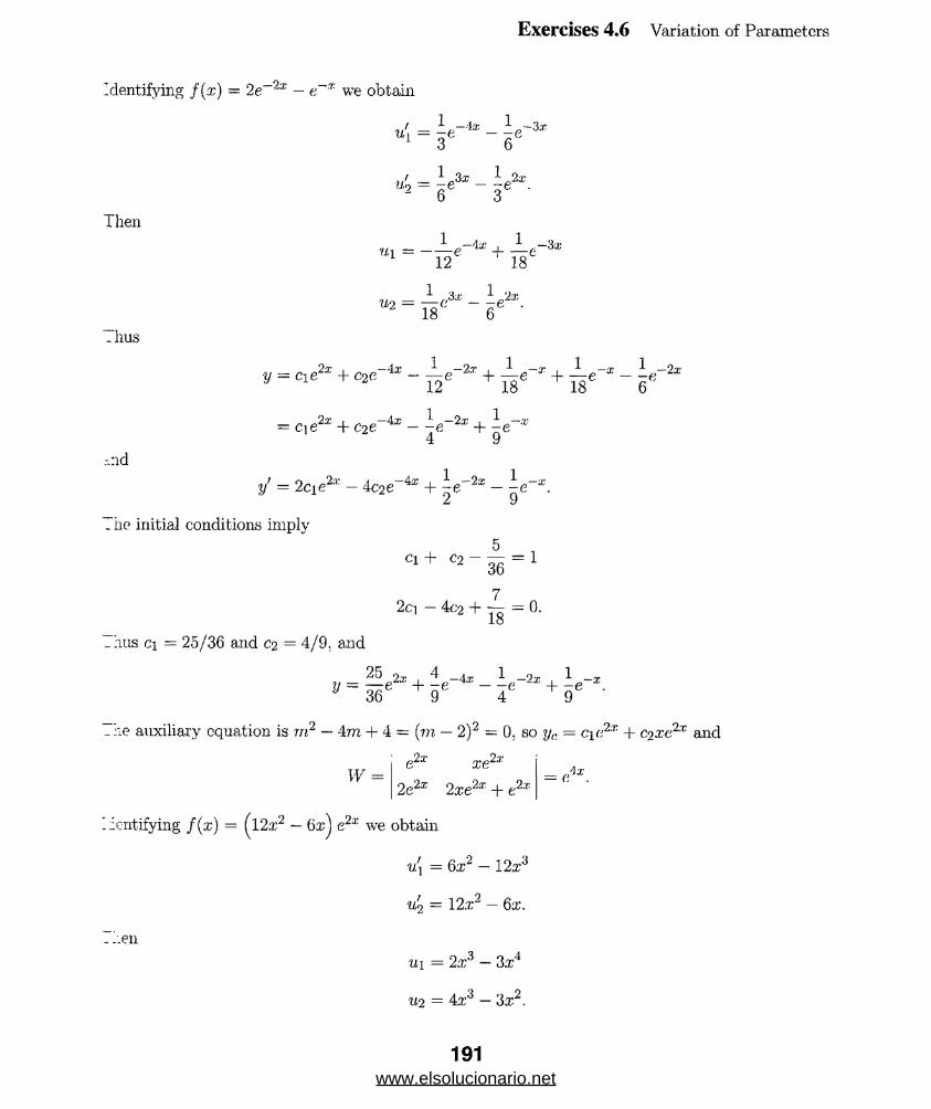
Exercises 4.6 Variation of Parameters
Identifying f(x) = 2e 2a: — e x we obtain
ut = L ;; -t* _ le-3® 3 6
1 3x ,2x
Then
“J = 6e
“ * = +
U2 = i , > _ ^ .
= cie2* + C2C,-4® _ l p-2a; + l g-x
.-.nd
j/ - 2c1e2'*' - 4c2e“4a: + V 2a 1z
. he initial conditions imply
9
Cl+ °2 _ 36 = 1
2ci — 4c2 + — = 0.
:hus ci = 25/36 and c2 =4/9, and
25 o, 4y = ^ e2* + -e~4* - -e-2x +
36 9
1 1
9
he auxiliary equation is m2 - Am + 4 = [m — 2)2 = 0, so yc = cie2* + coxe2x and
■2x
W =2r
2e2iC 2,'ce2* + e2x
ientifying /(&•) = (12a;2 — e2x we obtain
v\ = (rx2 - 12x3
«2 = 12.r“ — 6x.
Then
til = 2x3 — 3rr4
'«2 = 4x’3 — 3x2.
= a4x
191www.elsolucionario.net
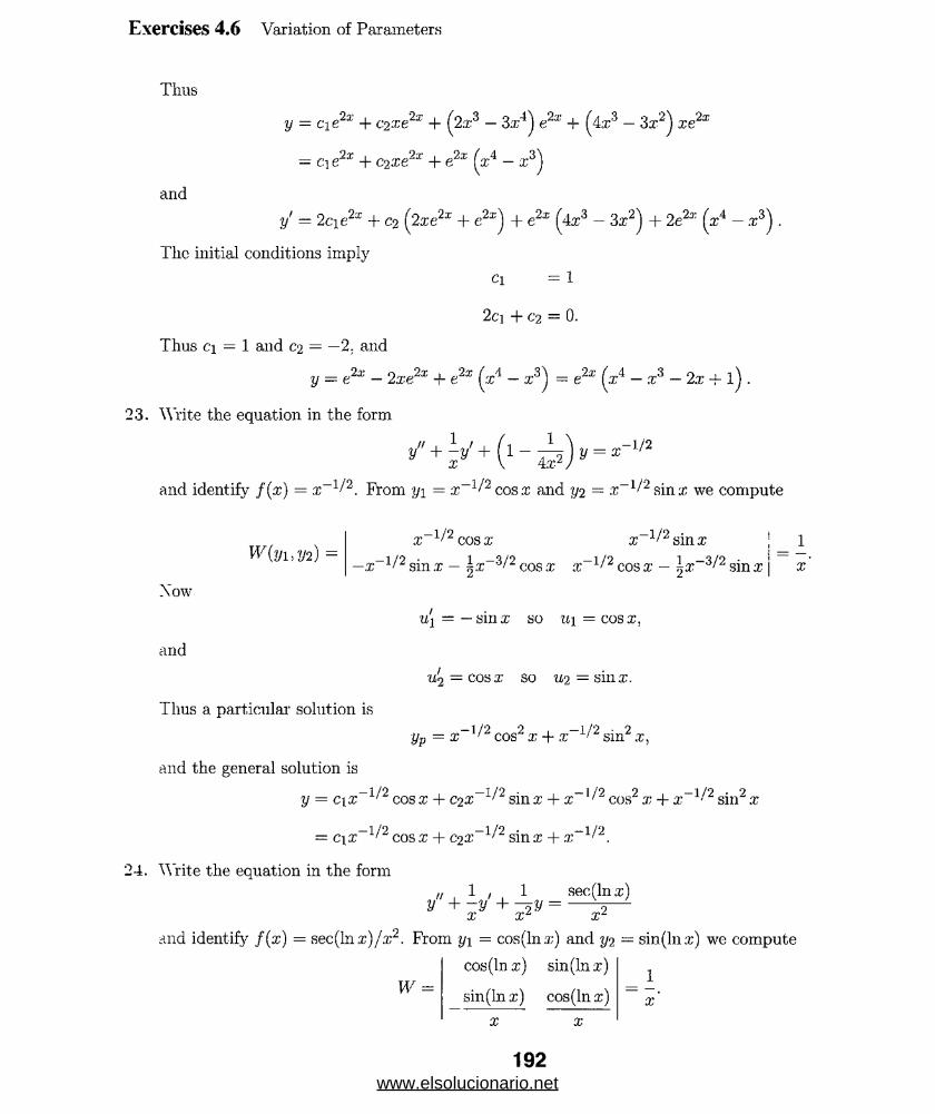
Exercises 4.6 Variation of Parameters
Thus
y = Cle2x + c2xelx + (2:r3 - 3x4) e2a! + (4x3 - 3x2) xe‘
— ci e2x + c2xe2x + e2x (x4 - x3)
and
y' — 2c\e2x + c2 (2xe2x + e2x) + e2x (4x3 - 3x2) + 2e2x (xA - x3) .
The initial conditions imply
Ci = 1
2ci + C2 = 0.
Thus ci = 1 and c2 = —2: and
y — e2x - 2xe2x + e2x (x4 - x3) = e2x (x4 - x3 - 2x -f l) .
23. Write the equation in the form
/ + i v ' + ( 1 _ _ L ) y = x - i /2
and identify f(x) = x-1/2. From yi = x-1/2 cosx and y2 - x-1/2 sinx we compute
W{yi,y2) =- 1/2.X / COSX
-X
x 1/2sinx ; 1
_1/2 sin x - 5X-3/2 cos x x-1/2 cos x - ^x-3/2 sin x j x ’
Xow
and
Thus a particular solution is
«1 = — sinx so « i = cosx,
u2 — cos x so u2 — S111.T.
yp = x 1//2 cos2 x + x 1/2 sin2 x,
and the general solution is
y = cix_1//2 cosx + C2X-1/2 sinx + x~1/2 cos2 x + x-1/2 sin2 x
= cix_1/2cosx + c2x_1/2 sinx + x“1/2.
24. Write the equation in the form,, 1 , 1 sec(lnx)
y + - y + — y = \ JX X L X L
and identify f(x) = sec(lnx)/x2. From ij\ = cos (lnx) and y2 = sin(lnx) we compute
W =
cos (lnx) sin (lnx)
sin(lnx) cos(lnx)
x x
1
x
192www.elsolucionario.net

Exercises 4.6 Variation of Parameters
Xow
and
, tan(lna’) iiq = ------- so = In ! cos(lnx)|.
x
1u'o = — so u-2 = In x.
x
Thus, a particular solution is
yp = cos(ln x) In | c.os(ln a;) J + (In x) sin(ln x),
and the general solution is
y = ci cos(ln x) + e2 sin(ln :r) + oos(ln a;) In | cos(ln :r) | + (In x) sin(ln x).
The auxiliary equation is m3 + m = m(rn2 + 1) = 0, so yc = ci + c-2 cos x + c% sin x and
1 cos x sin x
W = 0 — sin x cos xiI 0 — cos x — sin x
Identifying f(x) = tan x we obtain
0 cos x sin x
u[ = W-\ = 0 — sin x cos x = tan x
tan x — cos x — sin x
= — sin x
= 1.
!1 0 sin x
«2= W2 = 0 0 COS X
0 tan x — sin x
1 C08 X 0
«3 = w:i = 0 — sin x 00 “ COS X tan x
= — sm x tan x —cosw x — 1
cosar= cos x — sec x.
Then
and
Hi = — In | cos a; |
U2 = cos x
«3 = sin x — In | see x + tan .r|
y = ci + C2 cos x + C3 sin x - In | cos x| -r cos2 x
+ sin2 x — sin x In j sec x + tan x \
= 0 4 + C2 cos x + C3 sin x — In | cos xj — sinx In | sec x + tan x\
193www.elsolucionario.net
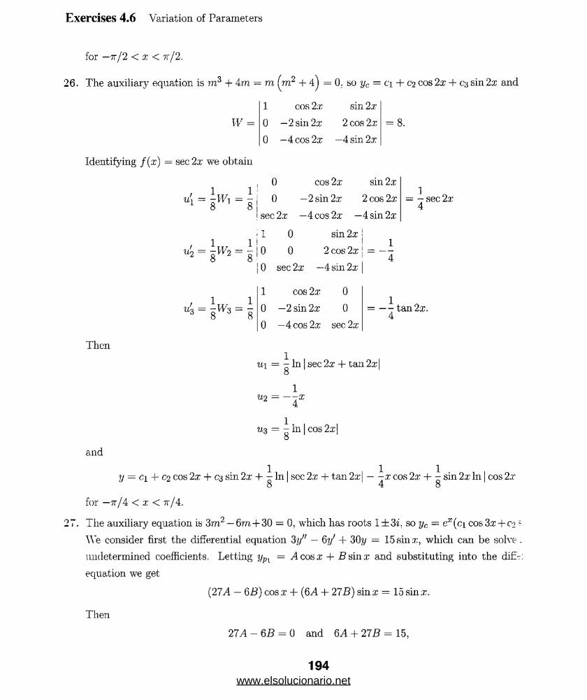
Exercises 4.6 Variation of Parameters
for — tt/2 < x < 7r/2.
26. The auxiliary equation is m 3 + 4m = m (rn2 + 4) = 0. so yc — a + co cos 2x + C3 sin 2x and
W =
1 cos 2 x
0 —2 sin 2 x
0 -4 cos 2x
sin 2 x
2 cos 2 x
-4 sin 2x
= 8.
Identifying f(x) = sec 2x we obtain
= lw'= i i0 cos 2 x sin 2 x
0 —2 sin 2 x 2 cos 2 x
I sec 2 x —4 cos 2 x —4 sin 2a'
0
0
— - sec 2 x 4
! 1 0 sin 2 x
U2 = l W2 = l\°| 0 sec 2 x —4 sin 2 x j
2 cos 2 x \ — —
u’s = iw 3 = i
1 cos 2rc 0
0 -2 sin 2 x 0
0 —4 cos 2x sec2x-
— — - tan 2 x.4
Then
•iti = - In | sec 2 x + tan 2 x\o
1«2 = —AX
«3 = - 111 | cos 2 x\ 8
and
1 . . 1 1 y = ci + C2 cos 2 x + C3 sin 2 x + - In | see 2 x + tan 2 x\ — -x cos 2 x + - sin 2 x In | cos 2 x
8 4 8
for —7r/4 < x < 7r/4.
27. The auxiliary equation is 3m2 — 6to + 30 — 0, which has roots l± 3i. so yc — ex(ci cos3x + c-± s.
\\’e consider first the differential equation 3y,r — 6 1/ + 30y = 15sinx-, which can be solve .
undetermined coefficients. Letting ypx = A cosx + B sin x and substituting into the difr-:
equation we get
(27A — QB) cosx + (6A + 27B) sinx = 15 sinrr.
Then
27A - 6 B = 0 and 6A + 27B = 15,
194www.elsolucionario.net
Exercises 4.6 Variation of Parameters
'O A = Yj and B = jL . Thus, yPl — ^ cosx + ^ sinx. Next, we consider the differential equation
■j/' — 6yr + 30y, for which a particular solution yP2 can be found using variation of parameters. The
’Yronskian isex cos 3x ex sin 3x
ex cos 3x — 3ex sin 3x 3ex cos 3x + ex sin 3xW =
identifying /(x) — jex tanx we obtain
t 1 . n 1 ( sitt2 3x \u-, = — - sm 3x tan-3x = — - -- — — —1 9 9 \ cos 3x J
1 ( l - cos“3x\ l / o o \- ---- --- = -~(sec3x — cos3a)9 I cos3x / 9 1
'"ext
iiius
1 1u\ = — — In ! sec 3.x + tan 3x1 + — sin 3x.
2y 1 27
/ 1 • . 1Uo = - sm3x so u-2 = — — cos 3.x. 2 9 27
1 ,Vp2 = ~ 2 j e’X cos On I sec 3x + tan 3x| — sin 3x) — — ex sin 3x cos 3x
= —— ex (cos 3x) In | sec 3x + tan 3x|Zi {
27
.-nd the general solution of the original differential equation is
y — e*(ci cos3x + o2 sin3x) + yPx{x) + yn {x).
The auxiliary equation is m2—2m+l = (m—l )2 = 0, which has repeated root 1, so yc = cicr+C2 xex.
’.Ye consider first the differential equation y" — 2yr + y = 4x2 — 3, which can be solved using
undetermined coefficients. Letting yPl = Ax2 + Bx + C and substituting into the differential
t:; nation wo get
Ax2 + (-4A + B)x + (2A - 2B + C )= 4x2 - 3.
. Hen
A = 4, -4 A + B = 0, and 2A-2B + C = -3,
i~j A = 4, B = 16, and C = 21. Thus, yPl = 4x2 + 16x + 21. Next we consider the differential
-quation y" — 2y' + y = x-1ex, for which a particular solution yP2 can be found using variation of
arameters. The Wronskian is
W =er xe
ex xex + ex= e2x
:!entifying f(x) = ex/x we obtain u\ — - 1 and u'2 = 1/x. Then u\ = —x and u2 — lnx, so that
yP2 = —xex + xex In x,
195www.elsolucionario.net
Exercises 4.6 Variation of Parameters
and the general solution of the original differential equation is
y = yc + Vpi + Vp-2 ~ cie',: ~ C2 xex + 4x2 + 16:r 4- 21 — xex + xex lux
= ci (f + c%xex + 4a;2 + 16a; + 21 + xex In x
29. The interval of definition for Problem 1 is (—tt/2. tt/2), for Problem 7 is (—oo, oo), for Pro
is (0, oo), and for Problem 18 is (—1, 1). In Problem 24 the general solution is
y = ci cos(ln.x) + c-2 sin(ln x) + cos (In x) In | cos (In x) | + (In a;) sin (In x)
for —tt/2 <\nx < 7t/2 or e_7r/2 < x < e?!2. The bounds on In a: are due to the presence of sc
in the differential equation.
30. We are given that y\ = x2 is a solution of xi y’1 + x3y' — Ax2y = 0. To find a second solution
reduction of order. Let y = x2u(x). Then the product rule gives
y' — x2u! + 2xu and y" = x2u" + 4xuf -f- 2u,
so
x4y" + x?y' — 4x2y — x5(xu" -f- bit) = 0.
Letting w = u’. this becomes xw' + 5w = 0. Separating variables and integrating we have
— — — - dx and In M = —5In:/; + c. w x
Thus, w — x~:> and u = —^x~4. A second solution is then tj2 = x2x~4 = 1/x2, and the -
solution of the homogeneous differential equation is yc = c\x2-\-Oi/x2. To find a particular
i/p, we use variation of parameters. The Wronskian is
n‘'2 1/x2 | 4
2x —2/x31 xW =
Identifying f(x) = 1/x4 wc obtain u[ = !> and u(2 = — \x l . Then u\ — —
U2 = - jlna;, so
Vv = ~ = ~ x ~ 2 -The general solution is
2 oi 1 1 ,V = ClX + ? - T 6 ? - 5 5 hl3:-
31. Suppose yp(x) = ui(x)yi(x) + U2 (x)y2(x), where tti and u-2 are defined by (5) of Section 4.1
196www.elsolucionario.net
Exercises 4.6 Variation of Parameters
rext. Then, for x and xq in I,
yT(X) - Vl(x) £ * + !*(*) £
= r -y\(x)y2 (t)f(t) df + rx yi(t)y2(x)f{t) ^
Jxo TV (£) Jxf)
- rJxq
W(i) Jx o W(t)
yi(*)^(g)/ft) ^ - 2/i(aQfft(*)/(*)
W'W W(t)dt
r yi{t)V2 {x)f(t) - y\{x)y2 {t)f{t) ^
Jxo W(t)
= r m i tJxo It [tj
= f G(x, t)f(t) dt.J xn
In the solution of Example 3 in the text we saw that y\ = ex, yo = <-: x, f(x) = 1/x, and W(y\. y-2) -
—2. From (13) the Green’s function for the differential equation is
ptp x __ pj-' p (*£G(xtt) = 1---- = sinh (a; - t).
The general solution of the differential equation on any interval [a:o, xj not containing the origin is
Men,r _T fx sinh(x — t) ,
■y = c\e + c2e + / ------- - dt.Jx o t
We already know that yp(x) is a particular solution of the differential equation. We simply need to
show that it satisfies the initial conditions. Certainly
l‘X o
/xo
Vsing Leibniz’s rule for differentiation under an integral sign we have
d f G ( x , t ) f ( t ) d t = r dIxo J x ()
7rom (13) in the text, G(x,x) = 0 so
d rx
'.To
.-.ud
y(xo) = I ° G(x,t)f(t)dt = 0.Jx 0it ion under an integral sign we
y'p(x) = - ^ jT G (z> t)f(t)dt = j -^G(x. t)f(t)dt + f(t)G(x, x) • 1 - f(t)G{x0, x) ■ 0.
V>p = Ix /t0
= it L ° GX"’ f ^dt = °‘197
www.elsolucionario.net
Exercises 4.6 Variation of Parameters
yp(x) = ( G(x, t)e2tdt,J 0
where G(x,t) = sinh (a; — t). Then
34. From the solution of Problem 32 we have that a particular solution of the differential equation
yp(x) — e2t sinh(x — t)dt = j~ e
= - T \ex+t - e~x+:it:2 Jo L
dt
d t = \ x+ t 1 -x+3t,2 3
= 1 2x _ 1 2« _ 1 « + 1 -* = l a * _ 1 + 12 6 2 6 3 2 6
Exercises 4.7I-' ■ •: ■ <v:’: • SVivIw ;;1 . . . .'■ . ■ • '• ; '. .7 • h;!:
1. The
2. The
3. The
4. The
5. The
6. The
7. The
8. The
9. The
10. The
11. The
12. The
13. The
,,2auxiliary equation is m2 — m — 2 = (m + l)(m — 2) = 0 so that y = c\x~x + c<ix
auxiliary equation is 4m2 — 4to + 1 = (2m — l )2 = 0 so that y = cix1/2 + C2X1/2 In x
auxiliary equation is to2 = 0 so that y = c.\ + c2 In x.
auxiliary equation is m2 — 4m = m(m — 4) = 0 so that y = c\ + c2x4.
auxiliary equation is m2 + 4 = 0 so that y = ci cos(2lnx) + C2 sin(2In x).
auxiliary equation is m2 + 4m + 3 = (m + l)(rn + 3) — 0 so that y — cix-1 + C2X-3,
auxiliary equation is rri2 — 4-rn — 2 = 0 so that y = cix2-'/® + c2x2+v .
auxihary equation is to2 + 2m — 4 = 0 so that y = c\x~l+s > -f c2x~1_v^.
auxiliary equation is 25m2 + 1 = 0 so that y = ci cos Q In xj + c2 sin ( l lnx).
auxiliary equation is 4m2 — 1 = (2m — l)(2m + 1) = 0 so that y = cix1'2 + c^x-1-'2.
auxiliary equation is m2 + 4m 4- 4 = (m + 2)2 = 0 so that y = c\x~2 + c-2 X~2lnx.
auxiliary equation is m2 + 7m + 6 = (to + l)(m + 6) = 0 so that y = c\x~l + c2x-6.
auxiliary equation is 3m2 + 3rn + 1 = 0 so that
f >/3 \ . fy/S ' c\ cos [ In x + C2 sin —— In x
14. The
6 ~~) ' 6
auxiliary equation is to2 — 8rn + 41 = 0 so that y = x4 [ci cos(51nx) + C2 sin(51n.x)].
198www.elsolucionario.net
Exercises 4.7 Cauchy-Euler Equation
m(m — l)(m — 2) — 6 = m3 — 3m2 + 2m — 6 = (in, — 3)(m2 + 2) = 0.
Thus
y — c\X3 4- C‘2 cos (V2 In x j + 03 sin (y/2 In x) .
Assuming that y == xm and substituting into the differential equation we obtain
m(m — l)(m — 2) + m — 1 ~ m3 - 3 m2 + 3m - 1 = (m - l )3 = 0.
Thus
y = c\x + C-2'X In x 4- C3x(lna;)2.
Assuming that y = xm and substituting into the differential equation we obtain
■n(m — l)(m — 2 )(m — 3) + 6 m(m — l)(m. — 2) = m4 — 7m2 + 6m = m(m — 1) (??7 — 2 )(m + 3) = 0.
Thus
y — c\ + cox 4- c$x2 + C4 X~'i .
Assuming that y = xm and substituting into the differential equation we obtain
■■Am — 1) (m — 2) (m — 3) 4- 6 m(m — 1) (m — 2) 4- 9rn(rn — 1) 4- 3m +1 = m4 + 2 m2 4-1 = (m2 +1)2 = 0.
Thus
y = ci cos(ln x) 4- C2 sin (In x) + oj (In x) cos (hi :r) 4- C4 (In x) sin(ln x).
The auxiliary equation is m2 — 5m = m(m — 5) = 0 so that yc = c\ 4 C2 Xr> and
1 a:5
0 5a;4
Assuming that y — xrn and substituting into the differential equation we obtain
K 4 = oar.
Identifying f(x) = a;3 we obtain u[ = - lxA and u'2 = 1/5*. Then ui = - ^ x 5, 112 = Aina;, and
y = ci + C2X0 — Jr .r ’ 4- \a:5 Ins = ci 4- c$xa 4- ln.r.2b 5 5
The auxiliary equation is 2m2 + 3m + 1 = (2m + l)(m + 1) = 0 so that yc = cyxr1 + c-2X~ 1 '2 and
W{x-X,x-V2) =a; ■ a - 1/ 2,,-1
- :r - 2 -Js-3/2= r f- 5/2.
! ::?ntifying f(x) — \ we obtain a[ = 1: - X1 and u'2 = x3 2 — x1/2. Then u\ = lx 2 — kx3;
. = 2^/2 _ p / 2, and
—1 —1 / 2 ^ 1 - 2 ^ 2 ^ —I —1/2 1 1 2y = CiX + C-2X + -x- -x + -X - = ClX + C x ' - -x + — X -
2 3 b 6 6 lt>
199www.elsolucionario.net
Exercises 4.7 Cauchy-Euler Equation
2X X.
1 2x= x2.
21. The auxiliary equation is m? — 2m -f 1 = (m — I )2 = 0 so that yc — C\x + c2x In x and
la; xlna; I I-v (x.xlnx) = j ; = x.
v ' ' |l 1 + In a; j
Identifying /(x) = 2/x we obtain Uj = —21nx/x and u'2 - 2/x. Then u\ - —(lna;)2, U2 = 2
and
y = C\x + C2 X In x — x(ln x)2 + 2x(ln a;)2
= cix + cox lna; + a.'(In x)2, x > 0.
22. The auxiliary equation is m2 — 3m + 2 = (m — 1 )(m — 2) = 0 so that yc - cyx -+ c2x2 and
W{x,x2) =
Identifying f(x) = x2ex we obtain - —x2ex and u'2 — xex. Then u\ = —x2ex + 2xex -
= xex — ex, and
y = c\x + C2 X2 — x3ex + 2x2ex — 2xex + x3ex — x2ex
— cix + C2 X2 + x2ex — 2xex.
23. The auxiliary equation m(m — 1) + m — 1 = rn2 — 1 = 0 has roots m i = —1, = -
- - ci a;-1 + C2 X. With y\ = a;-1. y2 = x, and the identification f(x) — lux/x2, we get
W = 2a;-1, W\ = — hi x/x, and W2 = In xfx3.
Then u[ = W\fW = —(lnx)/2, = W2/W = (lna;)/2x2, and integration by parts gives
u\ = ^x — -x 111 x £ z
1 - ll 1-1 U2 = —~x In x — -x .2 2
yp = uryi + U2V2 = Qa; - ^xlnx^ x_1 + ( - ^ -1 lnx - x = - lnx
y = yc + y-p — e j x - 1 -f- c^x - l n x , x > 0.
24. T .e auxiliary equation m(m — 1) + m — 1 = m2 — 1 = 0 has roots rm = —1, =
. • = f ix-1 + C2X. With yi = x_1. y-2 = x, and the identification /(x) = l/x 2(x + 1), we get
W = 2x“\ Wi = -1 fx(x + 1), and = l/x 3(x + 1).
200www.elsolucionario.net

Exercises 4.7 Cauchy-Euler Equation
Then u'i = W\/W = —l/2(x + 1), u2 = W2 /W — lj2x‘1(x + 1), and integration (by partial
fractions for u2) gives
50
and
m
U2
~2 + 1)
^lnrr + ^ln(a: + l),
Vp = U-m + U-2V2 =1
ln(a; + 1) x 1 + 1 -1 1 , /~ 2 X — 2 9
X
1 1 , 1 , , ln(.-r + 1) 1 1 / 1\ ln(x + l)= ~ - -2x ln x + ^x \n (x + 1) - ^ — 11 = __ + _,;ln (1 + _)
2x
- 1 1 1 , ln(x+l)= Vc + Vp = ci a: + e2x - - 4- -xln 1:1 + - J ----—— x > 0.
The auxiliary equation is m2 + 2m = rn(m + 2) = 0, so that y = c.\ + c2x 2 and
/ = —2c2-'E~3. The initial conditions imply
ci + C2 = 0
- 2 c 2 = 4 .
Thus, ci = 2. c2 = —2, and y — 2 — 2a;-2. The graph is given to the right.
yn
-1.0 —
-20
-K
rhe auxiliary equation is m2 — 6m + 8 = (m, — 2)(m — 4) = 0, so that
y = Cix2 + c2x4 and y' = 2cix + 4c2.t3.
Tae initial conditions imply
4ci -i- 16c2 = 32
4ci + 32c2 = 0.
. :ius, ci = 16. c*2 = —2, and y = 16a;2 — 2x4. The graph is given to the right.
201www.elsolucionario.net

Exercises 4.7 Cauchy-Euler Equation
27. The auxiliary equation is m2 + 1 = 0. so that
y = ci cos (In x) + c-2 sin(ln x)
and1 1
y' = —ci — sin (In x) + Oz~ cos (In a;).it .2/
The initial conditions imply ci = 1 and C2 = 2. Thus
j = cos (In x) + 2 sin (In x). The graph is given to the right.
J*
l\H .l-f -!-l-50
2S. The auxiliary equation is m2 — 4m + 4 = (in — 2)2 = 0, so that
y = c\ x2 + C2 X2 hi x and y' = 2c\_x + (x + 2x In a;).
The initial conditions imply ci = 5 and (>i -t-10 = 3. Thus y = bx2 — 7x2 lu x. The
graph is given to the right.
y
5 --/■
- i o —
-20
-30 -r
W (l, ln;r) =
29. The auxiliary equation is rri2 = 0 so that y<: = c\ + C2 hi a; and
1 In ;r | 1
0 l/x\ x
Identifying f(x) = 1 we obtain u[ = —x hi a; and ih = x. Then
?./i = j a:2 — \x2 In x. U2 = ?x2, and
y = ci + C2 In x + -x2 — ^a;2 In x + -x2 hi x = c\ + C2 In x + ^.t2.
The initial conditions imply ci + 1 = 1 and cj + ^ . Thus, ci = | , C2 =
and y = | — In a; + |a:2. The graph is given to the right.
- 1,
yi 15 —
10
5 —
3U. The auxiliary equation is rri2 - 6rn + 8 = ( m — 2)(777. — 4) = 0, so
that ijc = C] x2 + C2 X4 and
W =x2 a;4
= 2x°.
0.05
2a; 4a;3
Identifying f(x) = 8x4 we obtain u\ = —4xA and u!2 = 4a;. Then 1
i': — —a;4, U‘i — 2a;2. and y — cyx2 + c^x4 + x6. The initial conditions imply
202www.elsolucionario.net

Exercises 4.7 Cauchy-Euler Equation
1 1 17C>1 Tr°2 ~ ~ 714 16 64
1 3
C, + 2C2 - “ lG-
Thus ci = ^ , 0 2 = — \, and y = j^x2 — + £6. The graph is given above.
Substituting x = a1 into the differential equation we obtain
The auxiliary equation is m2 + 8m — 20 = (m + 10) (m — 2) = 0 so that
y = cie~m + C2e2* = ci£-10 + c2:r2.
Substituting x = into the differential equation wc obtain
The auxiliary equation is m2 — 10m + 25 = (m — 5)2 = 0 so that
y — cie5< + C2 teu = ei&'° + C2.x5 lnx.
Substituting x = e* into the differential equation wc obtain
i l + g'JV + g , ( , = e2< d t?+ dt “
The auxiliary equation is m2 + 9rn + 8 = (m + l)(m + 8) = 0 so that yc = cie_< + C2e~84. Using
undetermined coefficients we try yp = Ae2t. This leads to 30_4e2t == e2t, so that A — 1/30 and
y = cier* + C2 e~8t + ^<?2/' = cix-1 + o2x~8 + ^ r :2.
Substituting x = et into the differential equation we obtain
d2y rdV , P _ o ++ % _ 2 t
The auxiliary equation is to2 — 5m + 6 = (rn — 2)(to — 3) = 0 so that yc ■ cic2t + c^e*1'. Using
undetermined coefficients we try yp = At + B. This leads to (—5.4 + (SB) + 6At = 2t, so that
.4 = 1/3. B = 5/18, and
9/ 0+ 1 5 o o 1 , O y = cie + c2e + 3 t + J g = CrX~ + °2X + 3 lllx‘ + ^8 '
Substituting x = el into the differential equation we obtain
203www.elsolucionario.net

Exercises 4.7 Cauchy-Euler Equation
The auxiliary equation is to2—4to+13 = 0 so that y,- = c2t{c\ cos3i+C2 sin 31). Using undetenr.
coefficients we try yp = A + Be*1. This leads to 13.4 + 10Be} = 4 -+■ 3e*, so that A = 4/13, B — c
,r.d
y = e2<(ci cos 3£ + C2 sin 3t) + — + z—e*I t j 1U
, , . 4 3
56. troni
follows that
= ar [ci cos(3 In x) + c2 sin(3 In x)} -+- — + — x.1 o 1U
d2y _ l_ (<Py_ _ dy\
dx2 x2 \ dt2 dt J
d?y __ 1 d ( d2y dy\ 2 / d2y dy\
dx3 a:2 \ dt? dt J x3 \ dt2 dt)I d / d2;t/\ I d / dy\ 2 d2t/ 2 dy
x2 dx \ dt? J x2 dx \ dt) x3 dt2 xs dt
1 d3t/ / 1\ 1 d2y / 1\ 2 d?y 2 dy
x2 dt3 Vx/ x2 dt? \av x3 dt2 x3 dt
_ 1 /d3y d2y
^■.ib.'titiiting into the differential equation we obtain
A _ 3 ^ + 2 ^ _ 3 ( ' ^ V _ ^ + 6 f6 !_6v = 3 + Mdt3 dt2 dt y dt2 dt) dt
<Py e d2y , - i i dV r, Q.-I** 5 ' " 6 ^ + 11* “ 6!/“ 3 + 3f'
7 :.r auxiliary equation is to3 — 6to2 + 11to—6 = (to— l)(m —2)(m —3) = 0 so that yc = c\et+c
Using undetermined coefficients we try yp = A + Bt. This leads to (11B — 6A) — 6Bt = -
::iat A = -17/12, B = - 1/ 2, and
t 21 ‘M 1 1 j. 9 3 I* 1 iy - c\e + c2e + c3e‘ ' - — - ~t = c-[X + c2x' + c3xJ - — - - In x.
":?xt two problems we use the substitution t = — x since, the initial conditions are on the ir~-
x. -| . In this casedy dy dx dy
dt dx dt dx
d2y d ( dy\ _ d f dy\ d . ,, __ dy' dx d2y dx d?y
dt? dt\ dtj dt\ dx J dt ^ dx dt dx2 dt dx2 '
204www.elsolucionario.net

Exercises 4.7 Cauchy-Euler Equation
The differential equation and initial conditions become
+ V = 0; y(t)t=1
= 2, y'(t) = -4.i=l
The auxiliary equation is 4m2 — 4 m + 1 = (2m — l )2 = 0, so that
y — cit1/2 + C2 t1/2 In i and y' = ^c ii-1^2 + C2 ^ i_1/2 + ^ •
The initial conditions imply ci = 2 and 1 + C2 = —4. Thus
y = 2t1/2 - 5i 1/2 In i = 2(-x)1/2 - 5(—a?)1/2 ln(-.x), * < 0.
The differential equation and initial conditions become
,2 c,2y
dt2 t=2= 8, ;v'(i) = 0 .t=2
The auxiliary equation is rri2 — 5m + 6 = (m — 2)(m — 3) = 0, so that
y = c i i 2 + C2i 3 a n d y' = 2c i t + 3c2i 2 .
The initial conditions imply
4ci + 8c2 = 8
4ci + 12c2 = 0
from which we find ci = 6 and C2 = —2. Thus
y = 6i2 — 2i3 = Gx2 + 2a:3. x < 0.
Letting u = x + 2 we obtain dy/dx — dy/du and, using the Chain Rule,
d2y d f dy\ d2y du rl2y , d2y
dx2 dx yciuy du2 dx dw2 du2
Substituting into the differential equation we obtain
o d2y du u2 - + u ~ - + y = 0 .
du2 d,u
The auxiliary equation is rn2 + 1 = 0 so that
y = ci cos (hi u) ■+• c'2 sin (In u) = ci cos [In (a; + 2)] + C2sin[In(x H- 2)].
If 1 — i is a root of the auxiliary equation then so is 1 + i, and the auxiliary equation is
(m — 2) [rn — (1 + ?)] [777 — (1 — ?)] = m3 — 4m2 + 6m — 4 = 0.
We need to3 —4 m2 + 6m —4 to have the form m(m — 1) (m — 2) + brn (rn — 1) + cm+d. Expanding this
last expression and equating coefficients we get b = — 1, a = 3, and d = —4. Thus, the differential
equation is
x\f - x V + 3xy' - Ay = 0.
205www.elsolucionario.net

Exercises 4.7 Cauchv-Euler Equation
41. For x2y" = 0 the auxiliary equation is m(m — 1) = 0 and the general solution is y = c\ + c--_
initial conditions imply c,\ — yo and c2 — y i, so y = yo + yi.x. The initial conditions are '
:or all real values of yo and y\.
For x2y" — 2xy' + 2y = 0 the auxiliary equation is rn2 — 3m + 2 = (m — l)(m — 2) = 0 a:,
general solution is y = cix + C2»2. The initial condition y(0) = yo implies 0 = t/o and the co:.
;/ 0) = yi implies c\ = yi. Thus, the initial conditions are satisfied for yo = 0 and for all real -
■ -yi-
F.'i’ ,r2yw — 4x;</ + 6y = 0 the auxiliary equation is to2 — 5m + 6 = (m — 2)(m — 3) = 0
i '-iieral solution is y = c\X2 4-c2x3. The initial conditions imply y(0) = 0 = yo and y'(0) = 0. .
■h- initial conditions are satisfied only for yo = yi = 0.
42. 7hv function y(x) =■ — -y/x cos(ln x) is defined for x > 0 and has ^-intercepts where lna; = 77 _ -
::r k an integer or where x — en/'2+k7r. Solving tt/2 + kir = 0.5 we get k ~ —0.34, so e,r//2+A'~
:: v all negative integers and the graph has infinitely many x-intercepts in the interval (0,0.”
43. The auxiliary equation is 2m(m — l)(m — 2) — 10.98m,(m — 1) + 8.5m + 1.3 = 0, ~.
= —0.053299, m2 = 1.81164, m3 = 6.73166, and
y = dX-0 0532" + CSX1’81164 + C3X6’73166.
44. Thr auxiliary equation is m(m — 1 )(m — 2) -f 4m(m — 1) + 5m — 9 = 0, so that m i = 1.4061.
two complex roots are —1.20409 ± 2.22291i. The general solution of the differential eqiuv..
y = ci.-r1'10819 + x_1:20409[c2 cos(2.22291 In x) + C3sin(2.22291 lnx)].
45. Fhv auxiliary equation is m(m — l)(m — 2) (m — 3) + 6m(m — 1) (m — 2) + 3m(m — 1) — 3m — -= =
?: :hat mi = m2 = V2 and m3 = m,4 — — \/2 . The general solution of the differential equat:
y = c jx ^ + C2 x ^ ln x + csx-" ^ + C4x_v^lnx .
46. 7hr auxiliary equation is m(m—l)(m —2)(m—3) —6m(m—l)(m —2)+33m(m—1) —105m+l<: -
-. :hat mi = m2 = 3 + 2i and m3 = ni4 = 3 — 2i. The general solution of the differential ecv.
y = x* [a cos(2 In x) + c2 sin(2 In x)] -1- x3 In x[c% cos(2 In x) + C4 sin(2 In x)].
4“. F;.t auxiliary equation
m(m — l)(m- — 2) — m(m — 1) — 2m + 6 = m3 — 4m2 + m + 6 = 0
roots mi = —1, m2 = 2, and m3 = 3, so yc = cjx-1 + c2x2 + C3X3. With yi == x-1, y-2 =
. — and the identification f(x) = 1/x, we get from (11) of Section 4.6 in the text.
W != x 3, W2 = -4, W3 = 3/x, and W = 12x.
206www.elsolucionario.net
Exercises 4.8 Solving Systems of Linear DEs by Elimination
Then u[ = W\/W = :r2/ 12, u? = W^jW = — l/3x, U3 = 1 /4r2. and integration gives
a?3 1 1u\ = U‘2 = -- In®. and u3 =
36 3 4,t
so
and
Vp = u m + U2V2 + u m =36
-1 +.„* + I » ( _ _ L ) = _ 2x2 _ l x 2 ] n I i
y = Vc + yp = Cix 1 + c2.'T2 + c3a;3 - jj.r2 - ^x2lnx, x > 0.
Exercises 4.8 • : : ■ ; ~ ' ' • • : ? L ; “ L i
.Solving.Systems Linear'BE&'by; ® r:;-:s I:?- 1'T;’ ■ ’ '•••; V'v c' v; • ;:v:".- ^' ..... ' * ' - ' -, ' ' - « ; .j i ' - « » . ...
From Dx = 2x — y and Dy = x we obtain y = 2x — Dx. Dy = 2Dx — D2x, and (D2 — 2D +1)* = 0.
The solution is
x = Cie1 + C2'tel
y = (ci - C2 )el + c2te*.
From Dx — Ax + 7y and Dy = x — 2y we obtain y = ^Dx — ix. Dy — \D2x — ^Dx, and
D2 — 2D — 1 5 )z = 0. The solution is
x = cie5t + c2e~3t
1 Kf _Q+y = -cic - c2e .
From Dx = —y -ft and Dy = x — i we obtain y = t — Dx, Dy = 1 — D 2x, and (D 2 + l)x = 1 + t.
The solution is
X = C l COS t + C2 s i l l t+ l+ t
y = ci sint — c2 cost -+-1 — 1.
From Dx — 4y = 1 and x + Dy = 2 wc obtain y = \Dx — | , Dy = \D2x. and (D2 + l)x = 2. The
- jlution is
x = c\ cos t + C2 sin t + 2
www.elsolucionario.net
Exercises 4.8 Solving Systems of Linear DEs by Elimination
5. From (D2 + 5 ) x — 2 y = 0 and — 2x + (D '2 + 2 )y = 0 we obtain y = ^(D 2 + 5)a,\ D2y = ^(D 4 + 5.
and (Z?2 + 1)(Z)2 + 6)x* = 0. The solution is
x = ci cos t -f- c-2 sin t + C‘3 cos VC t + C4 sin \/61
y = 2 c\ cos t + 2 c.2 sin t — ^ 3 cos V(i 4 sin \/61.
6. From (D + l)x + (D — 1 )y = 2 and 3.r + (D + 2 )y = —1 we obtain x = — | -
Dx = — \{D2 -f 2D)y, and (D2 + 5)y — —7. The solution is
7
y = ci cos \/51 + C2 sin V5 f — -0
/ 2 Vo \ /V5 2 \ . /- 3a; = I - -ci. — — C2 I cos vo t + I "g-ci — ^°2 j sm 5 '
7. From D2x = Ay + ef and D2y - Ax — e* we obtain y — \D2x — ^el . D2y = \DAx — \el, and
(D 2 + A)(D — 2)(D + 2)x = —3e{. The solution is
x - ci cos 21 + C2 sin 21 + c e2t + 04c:_2f -h ^ef5
y = —ci cos 21 — C2 sin 2 t + c^e21 + 04c-2* — -e*.5
From (D 2 + b)x + Dy = 0 and (D + l)a? + (D — A)y - 0 we obtain (D — 5)(D 2 + 4)x =
D — 5)(D 2 + 4)y = 0. The solution is
x = C] eot + C2 cos 21 + C3 sin 21
y = c.4 eot + c-y cos 21 + c.q sin 21 .
Substituting into (D + l)<r + (D — A)y = 0 gives
(6ci + c±)eot + (02 + 2c3 - 4c5 + 2cq) cos 21 + (-2c2 + C3 — 2c’5 - 4ce) sin 2 t = 0
50 that 04 = — 6ci, cr} = 5 C 3 , cq - —\ c i . and
r 1 1y = — 6cie + -C3 cos 21 — ~C2 sin 21
Zi £i
?. From Dx + D2y = irit and (D + l)x + (D — 1 )y = Ae'il wc obtain D(D 2 1)* = 34t;-
D D 2 + 1 )y = - 8 e:it. The solution is
4V = ci + c2 sm t + C3 cos t — — e
lo
17 o,X = C4 + C5 S ill t - r C(i cos t + — e .
15
.r instituting into (D + l);r + (D — 1 )y = 4e'w gives
(c,-i — cj) + (cs — C(; — C3 - C2) sin t + (eg + cr, + C2 - c3) cos I = 0
208www.elsolucionario.net

Exercises 4.8 Solving Systems of Linear DEs by e_1:
so that C4 = ci, c'5 = c.3 . cq = — C2- find
17x = ci — co. cos t + ca sin t + ^-e3t.
15
lit. From D2x — Dy = i and (D + 3)& + (D + 3)y = 2 we obtain D(D + 1)(D -f- 3)x = 1 + St and
D(D + 1 )(D + 3);;/ = —1 — 31. The solution is
x = ci + c-2e_t + c%e~M -t+ \ t2
1y — C4 -+- Coe f + cgc + £ — — t2.
Substituting into (D + 3)x + (D + 3)y = 2 and D2x — Dy — t gives
3(ci + C4) + 2(c<2 + cj)e = 2
and
(c2 + cs)e_i 4- 3(3c3 + C6)e_,it = 0
so that C4 = — ej, eg = — C2, c& = S C 3 . and
y = —cj — C2e-f — 3c3e~’ + i — ^f2.
11. From (D2 — l)x — y = 0 and (D — l)x + Dy = 0 we obtain y = (D2 — l)x, Dy = (D* — D)x, and
1D — 1)(D2 + D + l)x = 0. The solution is
x = cie4 + e il 1a/3 . \/3 '
C'2 cos — t + c3 sm — t
( 3 a/3 \ _ ,/2 A (yft 3 \ _ t/9 .
» = ( - 5« - T e» j e C0ST t + ( T C2' H e lnT
I I . From (2D 2—D —l)x —(2D+l)y = 1 and (D— l)x+Dy - —1 we obtain (2D+1)(D—l)(D+ l)x = —1
and (2D + 1)(D + 1 )y = —2. The solution is
x = cie~f/2 + C2 e~t + eje1 + 1
y = C4e_f,/2 + cr,e_< — 2.
Substituting into (D — l).r + Dy = — 1 gives
(~ 5c;i ~ \°4) c~t/2 + _ 2 °2 ~ Cr e~# = 0
so that 04 = — 3ci. Cf, = — 2c2, and
y = — 3cie —2c‘ie~t - 2.
209www.elsolucionario.net

Exercises 4.8 Solving Systems of Linear DEs by Elimination
13. From (2D—5)x+Dy = e1 and (D—l)x+Dy = 5ef we obtain Dy = (5—2D)x+et and (4—D)x =
Then
u 4 t x = cieu + -eO
and Dy = — 3ci<34* -f 5e1 so that
y = -~Ac\eu + C2 + 5e*.
14. From Dx+Dy = ct and (—D'2 +D+l)x+y = 0 we obtain y = (D 2 — D — l)x, Dy = (D?‘ — D 2 — .
and D2(D — l)x = ef\ The solution is
x — Ci + C2 t + c^e1 -r te4
y = -ci — c-2 — cat - cze*' - tet + ef.
15. Multiplying the first equation by D + 1 and the second equation by D2 + 1 and subtractir.:
obtain (D4 — D2)x — 1. Then
x = ci + C2 t + c%el + C4 e~f’ — 12.
Multiplying the first equation by D + 1 and subtracting we obtain D2(D + 1 )y = 1. Then
-/ 1y = c5 + cet + c7e - -t-.J-t
Substituting into (D — l)x + (D2 + l)y = 1 gives
( — C i + C2 + C5 — 1) + ( — 2C4 + 2 C f ) e * + ( — 1 — C-2 + — 1
so that = ci — c2 + 2. c$ = C2 + 1, and Cf = 0 4 . The solution of the system is
x — ci + C2t + c^e1 + c.ie_t — ]-t2.z
y = (ci - c2 + 2 ) + (c2 + 1 )t + c4e~1 - ^ t2.
16. From D2x — 2(D2 + D)y = sin t and x + Dy = 0 we obtain x - —Dy, D 2x — — D 3;.
D(D2 + 2D + 2 )y = — sin t. The solution is
1 2y — c\ + C2 e~t cos t + cge-* sin t + - cos t+ - sin t
0 5
x = (c2 + 03)6 4 sin t + (02 - 03)6 1 cos t + - sin t — - cos t.0 0
17. From Dx = y, Dy — z. and Dz = x we obtain x — D2y = D^x so that (D — 1)(D2 + D + 1
t -t/i . V s 'x = cie + e C2SUI — t + C3 cos —-t
Z Z1
210www.elsolucionario.net

Exercises 4.8 Solving Systems of Linear DEs by Eliminatio::
t . ( 1 \ / 3 y = cje'+ I -~c2 - — c;
and.t ( 1 \/3
s = ce- + I — <* + -
3j '• 4/2 sm + ( y U - h '3 j <- ,/2 cos
<*) c-^2 sin ^ + (- c 2 - ic 3) <r</2 cos
IS. From .Dx + z = e*, (D — l)ar + Dy + Ds = 0; and x + 2y + Dz = e) we obtain z = —Dx + f .
Dz = —D2x + et, and the system (-D2 + D — l)x + Dy = —ef and (-D2 + l)x + 2y = 0. The::
y = \{D2 — l)a\ Dy - ^D(D2 — \)x, and (D — 2){D2 + l)x = — 2e* so that the solution is
9/ /x = c\ e + c-2 cos t + C3 sin t + <r
y = jjcie2* — C2 cost — C3 sin tLi
z = —2cie2* — C3 cos t + C2 sin t.
-1-. Write the system in the form
Dx - 6y = 0
x — Dy + z = 0
x + y - Dz = 0.
Multiplying the second equation by D and adding to the third equation we obtain
D + l)x — (D2 — l)y = 0. Eliminating y between this equation and Dx — 6y = 0 we find
{D3 - D - 6 D - 6)x = (D + 1)(D + 2)(D - Z)x = 0.
Thus
x = c\e~f + C2 &~2t + c^e3t7
and, successively substituting into the first and second equations, wo get
1 -t 1 -n 1 vV = —xcie - ~c2.e u + -c3e'6 3 2
^ — t 1 —21 1 3fz = ~fcie ~ r>C2 e 2t + -c-ieM.
6 3 2
- "A rite the system in the form
(D -)■ — z — 0
{D + l)y - z = Q
x — y + Dz = 0.
Multiplying the third equation by D + 1 and adding to the second equation wTe obtain
D + l)x + (D2 + D — 1 )z = 0. Eliminating z between this equation and (D + l)x — z = 0
211www.elsolucionario.net
Exercises 4.8 Solving Systems of Linear DEs by Elimination
--■= find D(D + l)2.r = 0. Thus
X = Cl 4- C2<?- t + c$te~l,
successively substituting into the first and third equations, we get
y = cj + (c2 - cs)e-t + c3te_<
z = c\ + C‘ie~l.
!1, 7r::n (D + 5)x + y = 0 and 4x — (D + l)y = 0 we obtain y — — (£> + 5):r so that Dy = —(D2-K-
T;-:: 4 j + (D2 + 5D)x + (D + o)x = 0 and (D + 3)2x = 0. Thus
x = cic~M + C2 te~M
y = —(2ci + c2)e~u - 2c2te~3t.
V'i-i .r(l) = 0 and y(l) = 1 we obtain
Cl 6 ~l~ C2C 3 — 0
—(2ci + c2)e~3 — 2 c2 C~3 = 1
Cl + C‘2 = 0
2ci -j- 3c2 = —e3.
= e* and c2 = —c?. The solution of the initial value problem is
x = e_3t_r3 - te~3t+3
y = —e-3t+3 + 2 te~3t+'\
2. Dx — y ~ —1 and 3a; + (D — 2)y - 0 we obtain x = —1(£> — 2)y so that Dx = —\{D2 — -
| i D2 — 2D)y = y - 1. and (D2 -2D + 3)y = 3. Thus
y = et (ci cos V2 i + C2 sin \/2 + 1
1 2 x = -ef‘ [(ci — V2 C2) cos \/2 i + (V2 ci + c2) sin \/2 + -.
'..'-i .• 0) = y(0) - 0 wc obtain
ci + 1 = 0
1 (C1- V 2 C2) + | = 0.
212www.elsolucionario.net
Exercises 4.8 Solving Systems of Linear DEs by Elimination
Thus ci = — 1 and c2 — V2/2. The solution of the initial value problem is
x = e* cos \/2t — ^ sin \/2tj
y = (>}■ cos y/2t -I- ^ sin \/2 + 1.
--3. Equating Newton's law with the net forces in tlie x- and ^-directions gives m d2 xjd£ 2 = 0 and
md2 y/dt2 — —mg. respectively. From mD2x = 0 we obtain x(t) — Cit+Co., and from mD2y = —mg
or D2y = —g we obtain y(t) = —\gt2 + c$t + C4.
24. From Newton’s second law in the .r-direction we have
d2x 1 dx . . dxm-r-n — —kcosv = —Ar— — = — c —
dt2 v dt 11 dt
In the y-direction we have
<Py , • a , ld V 1 I dym-r* ~ —mg — k sm 6 = —mg — k— — = —mg — c — .
dt2 J y vdt ' 'dt
From mD 2 x+ \c\Dx = 0 we have D(mD + \c\)x — 0 so that (mD + |c|)x = ci or (D + \c\jm)x — .
This is a linear first-order differential equation. An integrating factor is ef = elclt/m so that
^ elcl^/m^] = \t/m
and e\c\l/mx = (c2m/|c|)e:Cl^m + C3. The general solution of this equation is x(t) = 0 4 + .
From (mD 2 + \c\D)y = —mg we have D(mD + \c\)y — —m,g so that (mD + |c|)y = —mgt + c\
or (D + \c\/m)y ~ —gt + 02- This is a linear first-order differential equation with integrating factor
eJ\c\dt/m = e \c\t/m.' Thus
d— = (-gt + c2)e|c|t/jl(JL 1/
e c\t/m.y = _ ^ 9 te\c\t/m + 7 ^ 9 e\c\t/m + t/m + ^ci
and
s'M = “ T ? (+ ~ r + c3 + C4«_ ic',/m-|c| cz
Z5. Multiplying the first equation by D + 1 and the second equation by D we obtain
D(D + l)x - 2D(D + 1 )y = 2t + t2
D(D + \)x — 2 D(D + 1 )y = 0.
This leads to 2t + t2 = 0, so the system has no solution.
213www.elsolucionario.net

Exercises 4.8 Solving Systems of Linear DEs by Elimination
26. The FindRoot application of Mathematica gives a solution of x\(t) — x2,{t) as approximate:
t = 13.73 minutes. So tank B contains more salt than tank A for t > 13.73 minutes.
27. (a) Separating variables in the first equation, we have dx\/x\ = —dtj50, so xi = Fr.
Xi(0) = 15 we get ci = 15. The second differential equation then becomes
= - f /5 0 _ 2 o r + _ L C9 = A e -« /5 0dt 50 75 2 ° dt + 75 2 10
This differential equation is linear and has the integrating factor cJ 2dt/'° = e2 '5. Then
_^r 2f/75 1 _ j* -t/50+2t/75 _ $ t / 1 5 0
dt[C X21 - 10 - 10e
so
e 2 l f7 5 X2 = 4 5 e t/ 150 + C2
and
*2 = 45e-,/5° + c2e-2,',re.
From x2(0) = 10 we get c.% = —35. The third differential equation then becomes
_ ? ® p -t /5 0 _ ™ -2 t /7 5 _ J _dt ~ 75 75 25
or
^ + i * , ... t -i/50 _ l i e-21/75dt 21> 5 lo
This differential equation is linear and has the integrating factor ef dt>2 = e*/2°. Then
^ .f t/25 1 _ 6 -t/b0+t/2b _ 11-24/75+^/25 _ 6 t/50 _ 14 */75
dt1* *3 j _ 5 15 “ 5 15 !
so
and
et/25:i'3 = 60e*/50 — 70ei//,a + 03
a* = 60c-*/m - 70e-2f/75 + cac-*/25.
From ;x’3(0) = 5 we get C3 = 15. The solution of the initial-value problem is
xi(t) = 15e-f/50
,-r2(£) - 45e"*/50 - 35e~2l'>7b
X3 (t) = 60e_t-/o° — 7Qe~ 2 1 ' 10 + 1 Se-^ 2'’.
214www.elsolucionario.net

Exercises 4.9 Nonlinear Differential Equations
I b) pounds sa lt
c) Solving xi(t) — t} , X2 (t) = | . and X3(t) = | . F iadRoot gives, respectively. t\ = 170.06min,
t-2 = 214.7min, and = 224.4min. Thus, all three tanks will contain less than or equal to 0.5
pounds of salt after 224.4 minutes.
Exercises 4.9 Nonlinear Differential Equations
"V? have y[ = y'{ = ex. so
(:v " f = (erf = e21 = v l
Also. y'2 = — sinx and y'{ — — cosx. so
{lh? ~ (- cosx)2 = cos2x = y i
H:-wever, if y = c\y\ + c y-i- we have (y,r)2 = {c\ex — C2Cosx)2 and y2 = (c\ex + 0 2 cosx')2. Thus " 0 / 2
" have y = y" = 0. so
yiy" = i-o = o = i(o)2 = ifej)2.’.so. y = 2x and y'l = 2, so
V2 V2 - ®2(2) = 2.r2 = ^ (2x)2 = ^(y£)2.
H.~ever. if y — c\y\ -f C2V2, we have yy" = (ci • 1 + c2x2)(ci ■ 0 + 2c2) = 2c2(ci + c2x2) and
: - Jfci • 0 + c2(2x)]2 = 2c|x2. Thus yy" ^ TjCy')2-
y = ?/ so that w/ = yw. The equation becomes vf = —u2 — 1 which is separable. Thus
du
- + 1= —dx = > tan « = —x -!-ci =>- y' = tan(ci — x) =>■ y = In | cos(ci — x)| + C2-
t/ = yf so that v! = y". The equation becomes u' — 1 + u2. Separating variables we obtain
du
1 + u‘= dx tan 1 u = x + ci u = tan(x + ci) = 4> y = — In | cos(x + ci)| + C2.
215www.elsolucionario.net
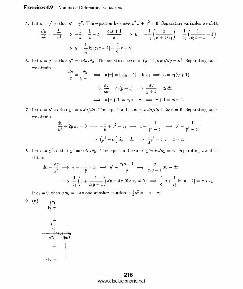
Exercises 4.9 Nonlinear Differential Equations
5. Let u = y' so that u' = y". The equation becomes x2u' + n? = 0. Separating variables we obtai:
du dx 1 1 _ cix + 1 _ 1 / x \ _ 1 / 1
u2 x2 « x Cl x 1 Ci ^x + l/c i/ ci \ci;r + l
=*> y = \ In |cix + 1|---x + Co.Cj_ Ci
6. Let 'u = y' so that y” = udu/dy. The equation becomes (y + 1 )udu/dy = «2. Separating vark
we obtaindu dy
■u y + 1In \u\ = In \y + 1| + In ci =>• u = c\(y + 1)
= , £ =<*(,+ !) =*. - $ ? = * « *ax y +1
In \y + 1| ~ c\x — C‘2 = » y + 1 = C3Cqx.
7. Let u = y; so that y" — udu/dy. The equation becomes udu/dy + 2yu3 = 0. Separating vari
we obtain
du . , 1 o 1 / I— + 2y dy = 0 =► — + r = d « = —--- =► y = -o---w2 u yl - ci y1 - ci
= » (y2 - ci) dy = dx =*• - ciy = x + c2.
S. Let. u = y' so that y" = udu/dy. The equation becomes y2udu/dy = u. Separating variab".:-
obtain
du = — = » u = -- + ci =^> ?/ = Ci;iy ~ 1 : y dy = fa y2 y '■ y cry - 1 '
1 / 1 \ 1 1 .— H ----- - dy = dx (for ci 7 0) =£• —y + — In I y — 1| = x + c .ci\ c j y- l J Ci q 1
If ci = 0, then y dy - —dx and. another solution is |y2 = —x + C2-
www.elsolucionario.net
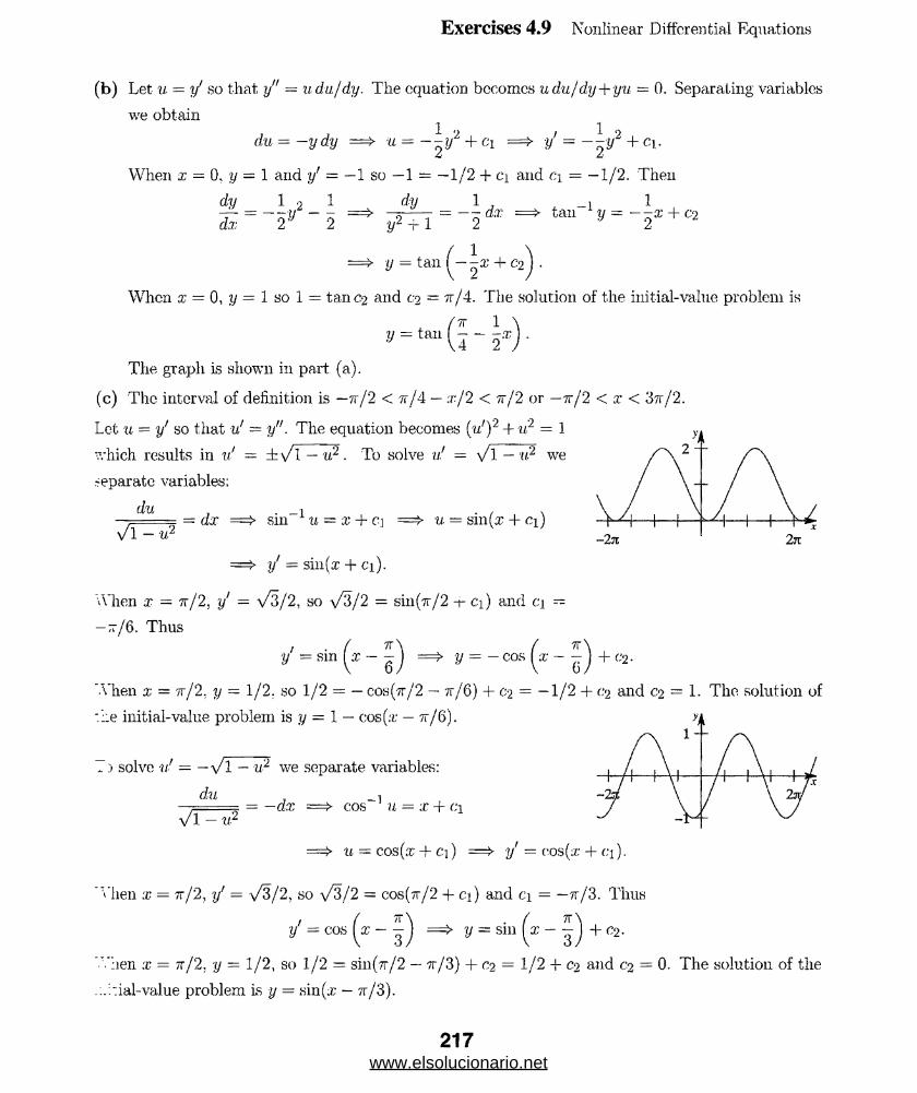
Exercises 4.9 Nonlinear Differential Equations
(b) Let u - y' so that y" = udu/dy. The equation bccomcs udu/dy+yu — 0 . Separating variables
we obtain
du = —ydy =
When x — 0, y = 1 and y' = —1 so —1 = —1/2 + c\ and c.\ = —1/2. Then
1 2 , 1 ,U = ~2V + 01 ^ V = + 01'
dy _ 1 2 1
dx 2V 2tan 1 y — --x + C-2
1
When x = 0, y = 1 so 1 = tanc2 and co, = tt/4. The solution of the initial-value problem is
y = tan ( I - ±x) .
The graph is shown in part (a).
(c) The interval of definition is —tt/2 < tt/4 — x/2 < tt/2 or —tt/2 < x < 3tt/2.
Let u - y' so that u' = y". The equation becomes (u1)2 + u2 = 1
which results in v! = ±\/l — u2. To solve u! = V l — «-2 we
separate variables;
du- dx sin 1 u = x + c u = sin (a; + ci)
V l^ u ?
=► y' = sin (a: + ci).
When x = tt/2, y — \/3/2, so \/3/2 = sin(7r/2 -j- c\) and c\ —
—tt/6 . Thus
-y = sm \x — — j i 67T
V = - COS ( ; £- - ) + C2.
When a; = tt/2, y = 1/2. so 1/2 = — cos (tt/2 — 7t/6) + ca = —1/2 + C2 and C2 = 1. The solution of
’ lie initial-value problem is y = 1 — cos (a; — 7r/6).
J S'solve u' = — \/l — u2 we separate variables:
fill -i
\/l — u2= —dx = > cos ‘ u = x + ci
=*► 'ii = COs(,T + C l) = = ^ ? / = CO s(;r + C l ).
Hien x = n/2, i/ : s/3/2, so \/3/2 = cos(tt/2 + c\) and ci = — tt/3. Thus
y = cos (a: - -7T
y = Sill ( X - - ) + C-2.
"nen x = t t / 2, y = 1/2 , so 1/2 = sin(7r/2 — -tt/3) + c2 = 1/2 -{- c2 and C2 = 0. The solution of the
_::ial-value problem is y = sin (a; — tt/3).
217www.elsolucionario.net
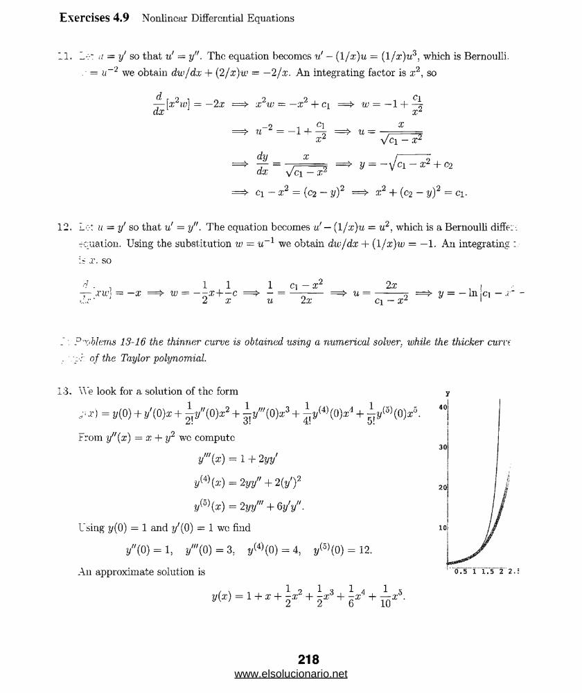
Exercises 4.9 Nonlinear Differential Equations
11. L->: a — y' so that v! = y". The equation becomes v! — (1 jx)u - which is Bernoulli.
. = t_r2 we obtain dw/dx + (2/x)w = —2/x. An integrating factor is x2, so
-j-[x2w] - —2x = > x2w = — x2 + ci =£• w = — 1 + ■% dx xz
—2 -[ , __ %u — — 1 -?— = > a =
X 2 y / c \ — X 2
dy xy = - \ j c i - X 2 + C2
dx \fc\ — x2
=*■ C l- x2 = (C2 - y f =*> X2 + (C2 - y f = Cl.
12. Lot u — y' so that v! = y". The equation becomes v! — (1 jx)u — u2, which is a Bernoulli differ:
rcuation. Using the substitution w - u_1 we obtain dw/dx 4- (l/x)w = —1. An integrating
..r. so
d . 1 1 1 c-[ — x2 2x , !— xw\ = - X = > W = -~X-i— c = * - = — ----- = > U = -------X = » y = - 111 j Cl - x- -cx • 2 x u 2x c\ — x1 1
?"obhms 13-16 the thinner curve is obtained using a numerical solver, while the thicker curve
of the Taylor polynomial.
13. We look for a solution of the form
x) = i/(0) + y'(0)x + ^y "( 0)z2 + ^-j/ff/(0)x3 + ^ l / 4)(0)®4 + ^ y (o)(0)z°-
From y"{x) = x + y2 wc compute
y"'(x) = 1 + 2 yy'
y(4)(a;) = 2yy" + 2 {y’f
y(°\x) = 2 yy’" + 6y'y".
Using y(0) = 1 and y'(0) = 1 wc find
2/"(0) = l, y'"(Q) = 3. 2/(4)(0) = 4, y^(0 ) = 12.
An approximate solution is
/ \ i 1 o ^ 3 ^ 4 I ty(x) = 1 + x + -x* + -x6 + -x4 + — a:0.
218www.elsolucionario.net

Exercises 4.9 Nonlinear Differential Equations
14. We look for a solution of the form
y(x) = y{0) + y'{0)x + ^ / ( 0)x2 + ^4!’ 5!'
From y"(x) = 1 — y2 we compute
y’"{x) = -2 yy'
yW(x) = -2yy" - 2(y'?
y^(x ) = - 2yy1" - fy/y".
Using y{0) = 2 and y'(0) = 3 we find
y"( 0) = —3, y"\0) = —12. t/4)( 0) = —6; 2/<5>(0) = 102.
An approximate solution is
y(x) = 2 + 3x~ ~x2 - 2:c3 - \x +2, 4 2i)
15. Wre look for a solution of the form
y(x) = y{ 0) + j/(0)x + y"{Q)x2 + i / ' ( 0)a;3 + ^ y {W (0).x'1 + ^?/{5) (0).*5.
From y"(x) = x2 + y- — 2y' we compute
ym(x) = 2x + 2yy' -2y"
y^(x) = 2 + 2{y')2 + 2yy" — 2y'"
y ^ ix ) - 6y'y" + 2yy'" - 2i/ 4K
Using y{0) = 1 and y'(0) = 1 we find
i/"(0) = - l, y"'{ 0 )=4 , ?/4)( 0) = - 6, y(5>(0) = 14.
An approximate solution is 0.5 1 1.5 2 2 .5 3 3.5
y(x) = 1 + x - -z1 + j *3 - jx 4 + - x 5.
219www.elsolucionario.net
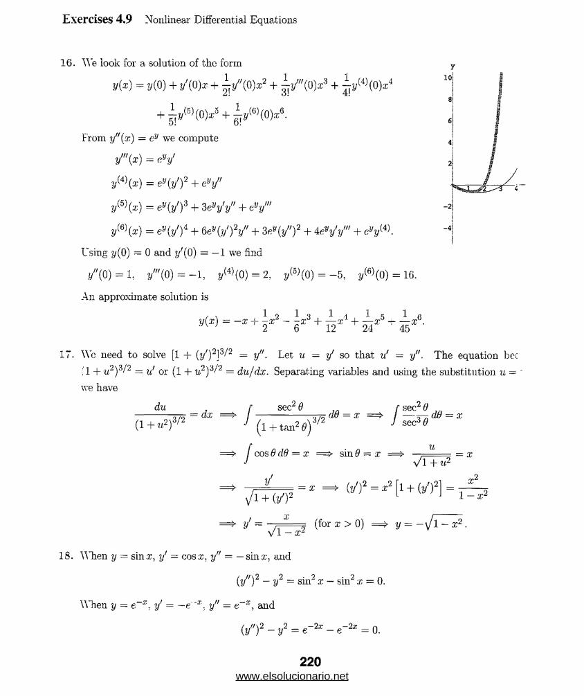
Exercises 4.9 Nonlinear Differential Equations
16. We look for a solution of the form
y(x) = y(0) + ■/fiij.r + j,y"(0)x2 +
+ I* M (0)*5 + i !,<<i>(0)z<’.
From y"{x) = ey we compute
y'"{x) = c V
y(4\x) = ey{yr)2 + eyy"
yW(x) = ey{y'f + 3evy'y" + eyym
y(6\x) = e»(j/ )4 + 6e V ) V + + Aeyy'y'" + eyy(4).
Using y(0) = 0 and ?/(0) = — 1 we find
/ ( 0 ) = 1, y '" (Q ) = — 1, y (4)(0) = 2, y ^ (0 ) = —5, 2/<6>(0) = 16.
An approximate solution is
/ S 1 9 1 ‘J '1 S 1 fjy ( x ) = _ x + - x - _ _ r + + _ r * + _ x < ,
IT. We need to solve [1 + (y02l3 2 = v"■ Let u = y’ so that u’ = >/'■ The equation bee
U + «2)3/2 = u' or (1 + u2)3/2 = du/dx. Separating variables and using the substitution u =
we have
du
(1 + n2f 2= dx I
Isec2 6 r sec2 9
( l + tan2*)372''<M=x
cos Odd = x =>• sin 9 ~ xu
y/\ + u2= a;
_ _ = i ^ ( ! / 0 2 = i 2 [ i + m 2 ] = _
(for x > 0) =£- y = —\J 1 — x2 .
~2
18. When y = sinx, y' — cosx, y" = — sinx, and
(y7/)2 — y2 = sin2 x — sin2 x = 0.
When y - e~x, j/ = —e"x. y" — e~x, and
(■y")2 — y2 = e~2x — e~2x = 0.
220www.elsolucionario.net
Exercises 4.9
From {y" ) 2 — y2 = 0 we have y" - ±y, which can be treated as two linear equations. Since linear
combinations of solutions of linear homogeneous differential equations are also solutions, we see that
:< = C]ex + C2 &~x and y = C3 cosx + c.4 sinm ust, satisfy the differential equation. However, linear
combinations that involve both exponential and trigonometric functions will not be solutions since
:he differential equation is not linear and each type of function satisfies a different linear differential
equation that is part of the original differential equation.
Letting a - y", separating variables, and integrating we have
du r r du— = \/l + uz — dx
Then
dx. and sinh 1 u = x + Ci.v/1 + u2
u = y" = s in h ( x + c i ) , y — co sh (.7; 4- c i ) + c.%, a n d y = s in h ( x + c \ ) - f c^ x + C3.
2*;. If the constant, — cf is used instead of cf, then, using partial fractions.
y = - f = --L f ( — ------ — ) dx = InJ x2 — Ci 2ci J \x — ci x + c\) 2ci
3; + C l
X — Cl+ C 2 .
Alternatively, the inverse hyperbolic tangent can be used.
21. Let u — dx/dt so that d?x/dt2 = udu/dx. The equation becomes udu/dx = —k2 /x2. Separating
variables we obtain
ku du = — 7; dx
x
1 9 k2-vr = — + c 2 x
1 2 k2
r = T +c-
"Alien t = 0, x = .to and v = 0 so 0 = (k2/x0) + c and c = —k?/xq. Then
L 2 = i? ( i - - ) and ^ =2 \x x q J dt \ x x q
separating variables we have
—, /- XX° dx = kV2 dt = > t V X() - x
".’sing Mathematica to integrate we obtain
- _I 1 9. ffcV 2 Jx
dx.x
t = - l ^ fcV 2
_ 1 [xq
~ f c V T
j \ xQ 2 x) j x- yj x (xq - x) - — tan ------ 1---
\/x■7-----v , a?o . -1 a?o - 2x:(x0 - x) + — tan ; f_
2 x \l X q — x
-2 x
2 ylx(xo - x)
221www.elsolucionario.net
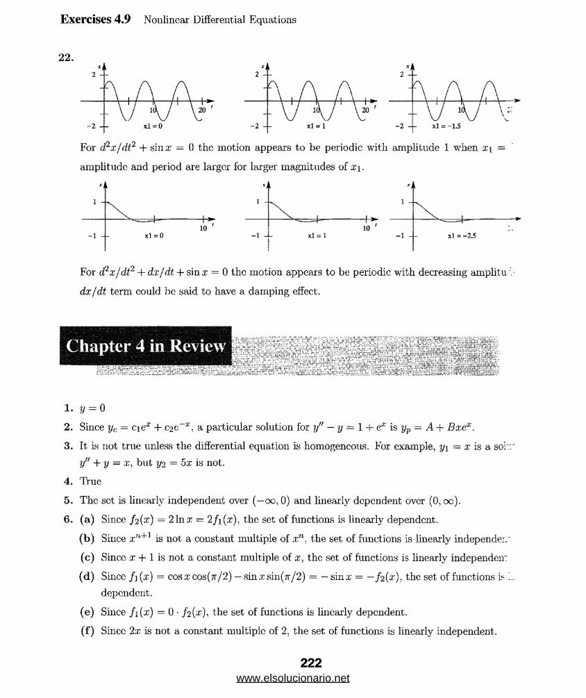
Exercises 4.9 Nonlinear Differential Equations
22.
For d2x/dt2 + sinx = 0 the motion appears to be periodic with amplitude 1 when x\
amplitude and period are larger for larger magnitudes of xi.
xi
1 -
k
1
1 1 1
xl =010 *
I
1 -
1 w
-1 - ■11 } I **
10 '
xi 1 -
-1 - xl = -2.5
For d?x/dt2 + dx/dt + sin x = 0 the motion appears to be periodic with decreasing amplitu
dx/dt term could be said to have a damping effect.
1. y = 0
2. Since yc = c.\ex + c-ic~x, a particular solution for y" — y — 1 + ex is yp = A+ Bxex.
3. It is not true unless the differential equation is homogeneous. For example, y\ = x is a sol'.'.'
y" + y = x, but tj2 = 5.x is not.
4. True
5. The set is linearly independent over (—oc, 0) and linearly dependent over (0, oo).
6. (a) Since f 2 (x) = 2 lnx = 2/i(x). the set of functions is linearly dependent.
(b) Since ,ru+1 is not a constant multiple of xn. the set of functions is linearly independei.'
(c) Since x + 1 is not a constant multiple of x, the set of functions is linearly independent
(d) Sincc/j(x) = cos x cos (tt/2) — sin x sin(-7r/2) = —sinx = — fzix). the set of functions is ...
dependent.
(e) Since fi(x) = 0 • /2(x), the set of functions is linearly dependent.
(f) Sincc 2x is not a constant multiple of 2. the set of functions is linearly independent.
222
www.elsolucionario.net

Chapter 4 in Review
(g) Since 3(:t2) + 2(1 — x2) — (2 + x2) = 0, the sot of functions is linearly dependent.
(h) Sincc xex+l + 0(4x — 5)ex — exex = 0, the set of functions is linearly dependent.
(a) The general solution is
y = c ie ix + C2 e~ ox + csx e~ 0X + c±ex + c~,xex 4- cqx2c x .
(b) The general solution is
y = c ix 3 + C2X~* 4- <%x~° ln x + c±x + c sx ln x 4- c%x(\nx)2.
Variation of parameters will work for all choices of g(x), although the integral involved may not
always be able to bo expressed in terms of elementary functions. The method of undetermined
coefficients will work for the functions in (b), (c), and (e).
From rn2 — 2m — 2 = 0 we obtain m = 1 ± a/3 so that
s = (.ie(i+v1 )I + C2e(i-vS)*
From 2m2 + 2m + 3 = 0 we obtain m = —1/2 ± (y/E/2)i so that
-x/2 ( \/5 . . \/5 \V = e ' I ci cos — x + C-2 sm — x I .
From ra3 + 10m2 + 25m = 0 we obtain m = 0, rn = — 5. and m = —5 so that
y = ci + c%e °* + (%xe ae.
From 2m3 + 9m2 + 12 m + 5 = 0 we obtain m = —1, rn = —1. and m = —5/2 so that
y = cie~Tyx'2 + C2e~x + C3xe~x.From 3m3 + 10m2 + 15m. + 4 = 0 we obtain m = —1/3 and m = —3/2 ± [\/l/2)i so that
y = c\e~xf* + e~*x/2 ^2 cos -a; + c3 sin -^:r^ .
From 2m4 + 3 m3 + 2m2 + 6m — 4 = 0 we obtain rn = 1/2. m = —2, and rn = ±y/2i so that
y = c\ex' 2 + C2 e~2x + C3 cos V2 x -f- C4 sin a/2 x.
Applying DA to the differential equation we obtain D‘1(D2 — 3D + 5) = 0. Then
ox/2 ( \/n . vT i \ ?. 3y = e ■> I ci cos — -x + C2 sm — -x j + C3 + ax + cgar + eg a;
y<:
and yp = A + Bx + Ca:2 + Dx*. Substituting yv into the differential equation yields
(5.4 - 3 B + 2C) + (5B - 6C + 6D)x + (5C - 9D)x2 + 5Dx* = -2x + 4a-3.
223www.elsolucionario.net
Chapter 4 in Review
Equating coefficients gives A = —222/625, D — 46/125, C — 36/25, and D = 4/5. The gei
solution isW 2 ( V l i . V ll \ 222 46 36 2 4 o
y = e: ^ cos _ * + c2 sm — xj - — + — * + - x + -*•.
16. Applying (D — l )3 to the differential equation we obtain (D — 1)3(Z> — 2D + 1) = (D — l )5
Then
y = ci<f + C2 xex + c$x2ex ■+• c ^ e * + c$x4ex .... v ^
Vc
and yp = Ax2ex + Bxi ex + Cx4ex. Substituting yp into the differential equation yields
12 Cx2ex + QBxex + 2Aex = x2ex.
Equating coefficients gives A = 0; B = 0, and C = 1/ 12. The general solution is
y - cje* + C2xex + ~^x4ex.
17. Applying D(D'2 + 1) to the differential equation we obtain
D(D2 + 1 )(D3 - 5D2 + 6D) = D2(D2 + 1 )(D - 2)(D - 3) = 0.
Then
y ~ pi + c%e + c.3e‘ ' + c±x + C5 cos x + cg sm x v r / yc
and yv = Ax + B cos x + C sin x. Substituting yp into the differential equation yields
6A + (SB + 5C) cos x + (—5B + bC) sin x = 8 + 2 sin x.
Equating coefficients gives A = 4/3, B = —1/5, and C = 1/5. The general solution is
S*r 4 1 1y = C\ + C2e“'' + C3<r + -x — - cos a: + - sinx.
3 5 5
IS. Applying D to the differential equation we obtain D(D i — D2) = D3(D — 1) = 0. Then
y = ci + c2x + csex + C4X2s - v-----'
Vc
and yp — Ax2. Substituting yp into the differential equation yields —2A — 6. Equating coeff.:
gives A = — 3. The general solution is
y = ci + C2:r + C3ex - 3x2.
19. The auxiliary equation is rn2 — 2m + 2 = [m— (l + «)][m— (1 —«)] = 0, so yc = c\ex sinx + cm
and
www.elsolucionario.net
Chapter 4 in Review
Identifying f(x) = ex tan x we obtain
, (ex cos x)(ex tan x)'"1 = ---- z-e-----= sin*
. (e:r sin x) (ex tan x) sin x 112 = ------------------ itz----- = ----- = COS x — sec X.
—elx cos x
Then u\ = — cos x, u2 = sin x — In | sec x + tana?|, and
y - cicx sin x 4- onf cosx — ex sin x cos x + ex sin x cosx — ex cos x In | secx + tan ar|
= c\cx sin x + C2 ex cos x — ex cos x In | see x + tan x\.
The auxiliary equation is to-2 — 1 = 0, so yc = aex + C2 e~x and
W =e x e xe x —e x
- - - 2 .
! identifying f(x) = '2ex/ (ex + e x) we obtain
U l e x + e ~ x 1 + e 2x03x
u2 — oX J_ p - X = —e"1 -t- e2x " ‘ l+ e2x'
Then ui = tan-1 ex, U2 = —ex + tan-1 e:r, and
y = c\ex + C2 e~x + ex tan-1 ex — 1 + e~x tan-1 ex.
The auxiliary equation is 6m2 — m — 1 = 0 so that
y — c\x1>/2 + C2 X~1/3.
The auxiliary equation is 2m3 + 13m2 + 24m + 9 = (to + 3)2(to + 1/2) = 0 so that
y = c\x~3 + C2 X~3 In x + czxr1'2.
The auxiliary equation is to2 — om + C = (m — 2) (to — 3) = 0 and a particular solution is
.. = x4 — x2 In x so thatcy i ) a
y = c:\x C2 X + x — x~ In x.
The auxiliary equation is to2 — 2to + 1 - (rn — l )2 = 0 and a particular solution is yp = ^x3 so that
i 3y = C\x + c.'ix In x + -x‘ .4
a) The auxiliary equation is to2 + J 1 = 0, so yc = c.\ cos ujx + oi sinuix. When u ^ a>
yp - A cos ax + B sin ax and
y = C] cos ivx + c‘2 sin ux + A cos ax + B sin ax.
225www.elsolucionario.net

Chapter 4 in Review
When u = a, yp = Ax cos oat + Dx sin ujx and
y — c\ cos iox + ci sin uix + Ax cos cox + Bx sin ux.
b) The auxiliary equation is rri2 — J 2 = 0, so yc — cie^x + C2 e~xx. When u ^ «, yp = Ae°'r
y = Clew* + c%e~wx + Aeax.
When u = a, yp = Axe°x and
y = cieMX + C2 e~u,x + Axeux.
26, (a) If y = sinx is a solution then so is y - cosx and rri2 + 1 is a factor of the auxiliary eqv.
m4 + 2m3 + 11m2 + 2m + 10 = 0. Dividing by rri2 + 1 we get m2 + 2m + 10, which has :
—1 ± 3i. The general solution of the differential equation is
y = cj cos x + C2 sin x + e~x (r% cos 3x + c.4 sin 3x).
(b) The auxiliary equation is m(m + 1) = m2 + m = 0. so the associated homogeneous differ-,
equation is y" + y' — 0. Letting y = ci + c2 e~x + \x2 — x and computing y" + yf we -
Thus, the differential equation is y" + 1/ = x.
27. (a) The auxiliary equation is m4 — 2m2 + 1 = (■rn2 — l )2 = 0, so the general solution .:
differential equation is
y = ci sinh x + c2 cosh x + C3X sinh x + C4X cosh x.
b ) Since both sinh x and x sinh x are solutions of the associated homogeneous differential eqv. ■
a particular solution of — 2 y" + y = sinh x has the form yp — Ax2 sinh x + Bx2 cosi;
25. Since y{ = 1 and y'[ = 0, x2y" — (x2 + 2x)y[ + (x + 2 )yi = —x2 — 2x + x2 + 2 x = 0, and y\ =
-olution of the associated homogeneous equation. Using the method of reduction of order. "
= ux. Then y' = xu' + u and y" = xu" + 2v!. so
x2 y" — (x2 + 2 x)y' + (x + 2 )y = x3 u" + 2 x2 u! — x3 u' — 2 x2v! — x2u — 2 xu + x2u + 2 x.
= x:iv" — xsv? = xs (u" — uf).
Tj find a second solution of the homogeneous equation we note that u = ex is a solu::
'' — u' = 0. Thus, yc = cjx + c-rxex. To find a particular solution wc set x:i(u" — u') =
u" — u' = 1. This differential equation has a particular solution of the form Ax. Substr
■"o find A = —1, so a particular solution of the original differential equation is yp - —x2
iviioral solution is y = c\x -j- C2xex — x2.
2 9. The auxiliary equation is m2 — 2m + 2 = 0 so that m — 1 ± i and y - ex (c\ cos x + c2 sin x). S
. - 2) = 0 and y(n) = —1 we obtain ci - e_7r and C2 - 0. Thus, y = e*-,rcosx.
226www.elsolucionario.net
Chapter 4 in Review
The auxiliary equation is m2+2m+l = (m+1)2 = 0, so that y = cie~x+c2xe~x. Setting y(—l) = 0
and y'(0) = 0 we get cie — c2e = 0 and —ci + c? = 0. Thus c\ = c-2 and y = c\{e~x + xe~x) is a
solution of the boundary-value problem for any real number ci.
The auxiliary equation is m? — 1 = (m — l)(w + 1) = 0 so that m = ±1 and y = c.\ex + c2 e~x.
Assuming yp = Ax + B + C sin x and substituting into the differential equation we find A = — 1,
5 = 0, and C — . Thus yp — —x — \ sin® and
y = c\ex + c2 e~x — x — - sin x.z
Setting y(0) = 2 and y'(0) = 3 wc obtain
ci + c-2 = 2
3 „Cl - C2 - - = 3.
Solving this system we find ci = -x and c2 = — § - The solution of the initial-value problem is
V13 5
4(ex — -e~x x — - sin®.
z*
The auxiliary equation is rn2 + 1 = 0, so yc — c\ cosx + c2 sin® and
cos x sin xW =
— sm x cos x= 1.
Identifying f(x) = sec3 x we obtain
, . o sm xux - — sin x sec x =
cos3 X
u'2 = cosx sec3 x = sec2 x.
Then1 1
ui = = —-sec ®2 cos2 x 2
Thus
u,2 = tan®.
y = ci cos ® + C2 sin x — - cos x see x + sin x tan xz
1 1 — COS2 X— ci cos x + c2 sm x — - sec ® H--------
2 cos x
aid
1= C3 cos x + (>2 sm ® + - sec ®.
Zi
227www.elsolucionario.net

i Chapter 4 in Review
/ • 1V = ~c3 sm x + c-2 cos x + - see x tail x.
initial conditions imply
:•! = C2 = 1/2 and
C3 + 2 = 1
1
C2 = 2-
y = - cos x + - sin x + - sec x.Z Z Z
13 1-" = y' so that u' — y". The equation bccomes u du/dx = 4x. Sepai'ating variables we obt
u du = 4x dx = > l~v2 — 2x2 + c\ = > u2 = 4x‘2 + c2. z
x = 1, y' = u = 2, so 4 = 4 4- 0 2 and c.2 = 0. Then
u2 = 4e2 =*• = 2x or ^ = -2 *ax
=£► y = x2 + C3 or y = —x2 + C4.
~ = 1. y = 5, so 5 = 1 + eg and 5 = —1 + o\- Thus eg = 4 and c& = 6. Wc have y = .
= — x2 + 6. Note however that when y = —x2 + 6. y' = —2x and y'{ 1) = —2 ^ 2. Thv.-
~ 1:::::: of the initial-value problem is y = x2 + 4.
k 1-' = so that y" = udu/dy. The equation becomes 2udu/dy = 3y2. Separating varial...
2u du = 3y2 dy =r- u2 = if1 + c i.
’ ' : = 0. y = 1 and y1 = u = 1 so 1 = 1 + c\ and c\ = 0. Then
2/ = , ( ^ ) = J. f x =yV 2 1r V2dv = dx
= > -2 i/_1/2 = * + C2 =*• y 4(x + c2)2 '
= 0. y = 1, so 1 = 4/c2 and c2 = ±2. Thus, y = 4/(re + 2)2 and y - 4/(rc — 2)-.
. that when y — 4/(x + 2)2, if = - 8/(r» + 2)3 and y'{0) = - 1 ^ 1 . Thus, the so'.".'
.r. value problem is y = 4/{x — 2)2.
T’:;f auxiliary equation is 12m4 + 64m3 + 59m2 — 23m — 12 = 0 and has roots —4. - -
r : 7=. The general solution is
y = ci(T<lx + C2 e~?>x' 2 + C‘ze~x,''i + c ^ x'2.
228www.elsolucionario.net
Chapter 4 in Review
I b) The system of equations is
27
IF
Cl + C-2 + ('3 -+- C'4 - -1
3 1 1= 2
2C2- 3 C3 +
2C4
9 1 1
4C2+ 9°3+
4C40
t 1 1= 0.■02 -
’ 27C3+
8C4
Using a CAS we find c\ = — , c2 = ^ , 03 = - 7 , and c.\ =
initial-value problem is
V- 4. IN -3*72 _ 3726 -*/3 + 257 /2-e H--- e
495 35 385 + i r “
Consider xy" + y' = 0 and look for a solution of the form y — xm.
Substituting into the differential equation we have
xy" + y’ - m(m — l).rTH'- 1 + rnxm~] = m2xm~].
Thus, the general solution of xy" + yf = 0 is yc = c\ -f c2 lnx. To find a
particular solution of xy" + 1/ - — \/x- we use variation of parameters.
The Wronskian is
W =
Identifying
*0 that
Then
1. In x
0 1/x
= — a1-1/2 we obtain
x ’^ ln x
1
x
-1
-2
- 3
-4
- 5
« i =1/x
-X~l/2= \/x. In x and xL = — — — = — y / x .
1/x
U'> =ui = In x — and
yv = x,i/2(^ lnx — — ^x3/2ln x = —k3 9 3
and the general solution of the differential equation is
y — c\ + c2 In x — ^x3/2.
The solution of the
229www.elsolucionario.net
Chapter 4 in Review
The initial conditions are y( 1) = 0 and i/(l) = 0. These imply that c\ = | and C2 —
solution of the initial-value problem is
4 2 1 4 3/9
The graph is shown above.
S~. From (D — 2)x -f (D — 2)y = 1 and Dx + (2D — 1 )y = 3 we obtain (D — 1 )(D — 2)y = —6
Dx = 3 - (2D - 1 )y. Then
3y = c\e2t + C2e* — 3 and x = —c^e1 — -cie2t + C3.
z
Substituting into (D — 2)x + (D — 2)y = 1 gives 03 = § so that
t 3 2t 5x = —coe-- cie H— .
2 2
3S. From (.D — 2)x — y = t — 2 and — 3x + (D — 4)y — —At we obtain (D — 1)(Z? — 5)rc = 9 — 81 T
t 5, 8, 3 x = aeS + c2e™ - -t - —
5 25:-L :i cl
1 c* 11y = (D — 2)x — t + 2 = + 3c2e5j!: + — 4- — t.
zo I d
39. From (D — 2)x — y = —el and —Sx + (D — 4)y = — 7et we obtain (D — 1 )(D — 5)x = —4e* so ‘
x = c\et + C2 <?yt + teK
Then
y — (.D — 2)x + e* = —ci 6 + 3c2G — tc*' + 26 .
40. From (D + 2)^ + (D + l)y = sin2i and 5x + (D+3)y = cos2£ wc obtain (D2 + 5)y = 2cos2i — T
www.elsolucionario.net

5 Modeling with Higher-Order Differential Equations
Exercises 5.1 Lmear Modelst Initial-Value Pwjblenits:r'.' “ ' ' ”' V - V;V: 'r.
; \ '' W , ” ' '' ; " ' V w,\ wJ\
1. From |x" + 16a: = 0 wc obtain
x — c\ cos 8\/21 + C-2 sin 8\f21
so that the period of motion is 2tt/8\/2 = \/2tt/8 seconds.
2. From 20a:'7 -f- kx = 0 we obtain
1 ik. . 1 [k
so that the frequency 2/tt = 5 y / 5 vr and k - -320 N/m. If 80a,’" -t- 320.x = 0 then
x = ci cos 21 + C2 sin 21
so that the frequency is 2/ 2tt = 1/tt cyclcs/s.
3. From ^x" + 72x = 0, a:(0) - —1/4. and ^(O) = 0 we obtain x = — cos4v61.
4. From |a:;/ + 72x = 0, ;r(0) = 0, and o/(Q) = 2 we obtain x = sin4\/6£.
!. From |;r" + 40a: = 0, a:(0) = 1/2. and a/(0) = 0 wc obtain x = | cosSi.
(a) x (tt/12) = —1/4, x(tt/8) = -1/2, x(7r/6) = -1/4, j;(7t/4) = 1/2, ^(9tt/32) = \/2/4.
(b) x' - —4sin81. so that ^(Stt/IG) = 4 ft/s directed downward.
(c) If x = cos 8t. — 0 then t — (2n -f 1)tt/16 for n = 0. 1, 2. . . . .
5. From 50a/' + 200x = 0. ;i‘(0) = 0. and x'(0) = —10 we obtain x = —5sin2t and x! = —10 cos 21
'• From 20:c// •+ 20a; = 0, a~(0) = 0, and aj'(0) = —10 we obtain x = —10 sin t and x/ = —10cost
(a) The 20 kg mass has the larger amplitude.
(b) 20 kg: x'(tt/A) = -by/2 m/s, 2/ (tt/2) = 0 m/s; 50 kg: :r'(7r/4) = 0 m/s, x'('x/2) - 10 m/s
(c) If —0 sin 21 = —10 sin t then sint(cos t — 1) = 0 so that t = nn for n — 0, 1. 2, ..., placing both
masses at the equilibrium position. The 50 kg mass is moving upward; the 20 kg mass is
moving upward when n is even and downward when n is odd.
231
www.elsolucionario.net
Exercises 5.1 Linear Models: Initial-Value Problems
8. From x" + 16x = 0. x(0) = —1, and a/(0) = —2 we obtain
x — — cos4t — ^ sin4t = sin(4t — 4.249).
The period is tt/2 seconds and the amplitude is \/5/2 feet. In 4tt seconds it will make 8 cor...
cycles.
9. From \x" + x = 0, x(0) — 1/2, and a/(0) = 3/2 we obtain
1 3 \/l3 ,x = - cos2t + - sin2t = —— sin(2£ + 0.588).
2 4 4
10. From 1.6x/; + 40.r = 0, z(0) = —1/3, and x''(0) = 5/4 we obtain
1 1 5 x = — - cos 5t + - sin 51 = — sin(5t — 0.927).
3 4 12
If x = 5/24 then t = g (| + 0.927 4- 2rwr) and t = i + 0.927 + 2mrj for n = 0, 1, 2, ... .
11. From 2x" + 200a; = 0. x(0) = —2/3, and a/(0) = 5 we obtain
(a) x = —| cos lOt + sin lOt = | sin(10t — 0.927).
(b) The amplitude is 5/6 ft and the period is 2tt/ 10 = tt/5
(c) 37t = -irk/b and k = 15 cycles.
(d) If x = 0 and the weight is moving downward for the second time, then 10£ — 0.927 = -'
t = 0.721 s.
(e) If x' = f cos(lOt - 0.927) = 0 then lOt - 0.927 = t t / 2 + mr or t = (2n + 1)tt/20 + 0.0.' -'
n = 0. 1, 2, ... .
(f) x{3) = -0.597 ft
(g) a/(3) — —5.814 ft/s
(h) ar"(3) = 59.702 ft/s2
(i) If x = 0 then t = ^(0.927 + mr) for n = 0, 1, 2 ,__The velocity at these times is
x' = ±8.33 ft/s.
(j) If x = 5/12 then t = j^(7r/6 + 0.927 + 2mr) and t = (57t/6 + 0.927 + 2wr) for n = 0. 1. .
(k) If x — 5/12 and xf < 0 then t = ^(5tt/6 + 0.927 + 2nir) for n = 0, 1. 2, ... .
12. From x,f + 9x = 0. .x(0) = —1, and x'(0) = —\/3 we obtain
, V3 - n 2 •x = — cos 3 t-- — sm 3t = —= sm3 VS
and x' = 2\/3cos(3i + 47r/3). If x' = 3 then t = —77r/18 + 2mr/3 and t = — t t / 2 + 2r~
n = 1, 2, 3, ... .
13. From k\ = 40 and k-2 = 120 we compute the effective spring constant k = 4(40) (120)/It --
Now, rri = 20/32 so k/m = 120(32)/20 = 192 and x" + 192a? = 0. Using a;(0) = 0 and a/(L
obtain x(t) = ^ sin8-\/3t.
232www.elsolucionario.net
Exercises 5.1 Linear Models: Initial-Value Problems
Let m be the mass and k\ and ko the spring constants. Then k = Ak\k2 i'(ki + k2) is the effective
spring constant of the system. Since the initial mass stretches one spring | foot and another spring
75 foot, using F = ks, we have = ^k2 or 2k\ — 3k2. The given period of the combined system
is 2t/uj = tt/15, so lo = 30. Since a mass weighing 8 pounds is 3 slug, we have from w2 = k/rri
302 = T^- = 4fc or k = 225.
We now have the system of equations
1/4
4A:i A’2= 225
k\ + k‘2
2k\ ~ 3k2.
Solving the second equation for k\ and substituting in the first equation, we obtain
4(3fc2/2)A~2 _ 12A| _ 12k2 ^
3fc2/2 -j- k2 5/c2 5
Thus, k2 = 375/4 and ki = 1125/8. Finally, the weight of the first mass is
fci 1125/8 375 32m = — = — —!— = — - « 46.88 lb.
o 3 8
I : For large values of t the differential equation is approximated by x" — 0. The solution of this
equation is the linear function x = c\t + c2. Thus, for large time, the restoring force will have
iecayed to the point where the spring is incapable of returning the mass, and the spring will simply
’-:?ep on stretching.
->i As t becomes larger the spring constant increases; that is, the spring is stiffening. It would seem
■hat. the oscillations would become periodic and the spring would oscillate more rapidly. It is likely
:hat the amplitudes of the oscillations would decrease as t increases.
1“ a) above ( b ) heading upward
!> a) below ( b ) from rest
11* a) below ( b ) heading upward
X. a) above ( b ) heading downward
H 7:om + x' + 2x = 0, x(0) = —1, and ^ ( 0) = 8 we obtain x = 4te~4t — e~‘lt and
= 8e_4f — 16te~4t. If x = 0 then t = 1/4 second. If x' — 0 then t = 1/2 second and the
•::treme displacement is x = e~2 feet.
1. ?:::>m \x” + \f2x' + 2x = 0, ,t(0) = 0, and ://(0) = 5 wc obtain x = 5te-2v2< and
233www.elsolucionario.net

Exercises 5.1 Linear Models: Initial-Value Problems
x' = be 2'^2 t( l — 2y/2tj. If x' = 0 then t — \/2/4 second and the extreme displacemcr.'
x = 5\/2 e_1/4 feet.
23. (a) From x" + 10;r' 4- 16a: = 0, x(0) = 1, and ^(0) - 0 we obtain x = — je -8*-
(b) From x" 4 x' 4 16x = 0. x(0) = 1, and ^'(O) — —12 then x = — §e_2t + ^e~st.
24. (a) x = |e-8* (4e6* — l) is not zero for t > 0; the extreme displacement is :/;(0) = 1 meter.
l b) x = (5 — 2e6*) = 0 when t = ^ln| w 0.153 second; if x' — fe-8* (e6< — 10) = 0 *.
t — | In 10 ~ 0.384 second and the extreme displacement is x = —0.232 meter.
25. (a) From O.Lz" 4 O.4.:?/ 4 2x — 0, x-(0) = —1, and x'(0) = 0 we obtain x = e~2t [ — cos4£ — 3 sir. -
\/K■ b) x = -~-e~2t sin(4£ 4 4.25)
z
(c) If x = 0 then 41 + 4.25 = 2tt, 3tt; 4tt, ... so that the first time heading upward is
t = 1.294 seconds.
26. ■ a) From |x" 4 x' 4 bx = 0, x(0) = 1/2, and ^(O) = 1 we obtain x = e~2t Q cos At 4 5 sin4~
b) x = - L e- 2‘ siB(4f + £ ) .c ) If x = 0 then At+n/A — 7r. 2tt. 37r, ... so that the times heading downward are t = (7+8n '
for n = 0, 1, 2, ... .
d) x ii1 \ j \
!/-If
2 7. rrom ffrxll+3x'+bx = 0 we find that the roots of the auxiliary equation are m = — §/3±|y4 J- -
a) If A32 - 25 > 0 then 0 > 5/2.
• b) If A32 - 25 = 0 then ,3 = 5/2.
• c) If A32 - 25 < 0 then 0 < (3 < 5/2.
2S. From 0.75a;" 4 3x' 4 6;r = 0 and 3 > 3\/2 we find that the roots of the auxiliary equation
234www.elsolucionario.net

Exercises 5.1 Linear Models
rn = — 13 ± \\j3? — 18 and
x = e~2 3 c\ cosh ^ \J0- — 18t + C-2 sinh \/i32 — 1813 v ' 3
If .r(0) = 0 and x'(0) = —2 then ci = 0 and oi = —3/\J32 — 18.
If \x" + \x' + 6.x = 10cos3f, r/;(0) = 2, and .x'(0) = 0 then
—i 12 ( V47 . . ^ }Xc = e ' Cl COS — t -i- C2 Sill — t2and xp = ^(cos 3t + sin 3t) so that the equation of motion is
, / 4 \/47 64 . V47 \ 10, 0 „* = e 72 f - - cos — £ - ^ j = sm — f J + — (cos 3£ sin 3t).
(a) If x" + 2x' + bx = 12 cos 2t + 3 sin 21, ;c(0) = 1, and ay(0) = 5 then xc = e *(ci cos 21 + ci2 sin 21)
and xp = 3 sin 21 so that the equation of motion is
x = e~l cos 2t + 3 sin 21.
(c) x
From x" + 8xf + 16:r = 8 sinAt. .2(0) = 0, and a/(0) = 0 wc obtain ;rr = c.\e 'u + ctfe u and
?p = — j cos 41 so that the equation of motion is
x — \e~il + te~ — 7 cos4i.4 4
From x" + 8x' + I62.’ = c_ tsin4i. x(0) = 0, and 2r'(0) = 0 we obtain xc = c-]_e~4t + C2 te~4i and
cos 41 — sin At so that
x = ^ g e_'U(24 + 100*) - ^ e_f(21cos4t + 7sin4t)-
As I —*■ oc the displacement x —»■ 0.
From 2x" + 32x = 68e~21 cos 4/;. x(0) = 0, and a/(0) = 0 we obtain x(: - cicos4t + C2sin4t and
n — \e~2i cos 41 — 2e~2t sin At so that
1 9 1x = —- cos At + - sin4t + -e~2t cos At — 2e~2t sin At.
2 4 2
'ince x = :sL L sin(4t — 0.219) — sin(4i — 2.897), the amplitude approaches \/85/4 as t —» 0 0 .
235www.elsolucionario.net

Exercises 5.1 Linear Models: Initial-Value Problems
35. i a)
■ b'l
By Hooke’s law the external force is F(t) = kh(t) so that mx" + fix' + kx — kh(t).
— / /■.,From \x" + 2x' + Ax = 20cost, ;.?;(0) = 0, and .^(O) = 0 we obtain xc = e (c\ c o s + co32 13
x — e
and xp = y| cos t + sin t so that
-2tl 56 ^ 72 . \ 56 32 .’ 1 — - cos 2t -- - sm 2t) + — cos t H— -sin 1
13 13 13 13
From 100a;// + 1600x = 1600 sin 81 x(Q) = 0, and x'(0) = 0 we obtain xc = c\ cos4£ + c;
and xp = — g sin 8t so that by a trig identity
2 1 2 2 x = - sin At — - sin 81 = - sin At — - sin At cos 41
3 3 3 3
If x = 5 sin4t(2 — 2 cos 4£) = 0 then t = nn/A for n = 0, 1, 2, ... .
I: x' — | cos4t—| cos8t = §(1—cos4£)(l-r2cos4£) = 0 then t = 7r/3+n7r/2 and t, = tt/6-
for n — 0, 1, 2. ... at the extreme values. Note: There are many other values of t for
j 7 = 0.
d i .n ~/6 + n-jr/2) = \/3/2 cm and x(-k/3 + rwr/2) — —\/3/2 cm
i e I x
b ■
C.i
3". rr::ir. x" + Ax = —5sin2t + 3cos2£, .r(0) = —1, and x;(0) = 1 we obtain xc = c\ cos21 +
= jt sin 21+ |£ cos 21, and
1 3 5x — — cos 2t — - sin 2t + —t sin 21 + -t cos 21.
8 4 4
35. r::,:n x" + 9:i: = 5sin 31 x(0) = 2, and x'(0) = 0 we obtain xc = c\ C0s3t + C2sin3t, xp = —
5 5x — 2 cos 3t + — sin 31 — '-t cos 31
18 6
3r>. a) From x!’ + u)2x = Fq cos7I x(0) = 0, and x/(Q) — 0 we obtain xc - ci cosuji + C2si::
xp = (Fq cos 7t)f (co2 — 72) so that
F0 Fo x —--~---» cos ut H— k---$ cos 71 .
u)z — 7Z — 7^
, , Fq —F()t sin j t Fq . b 1 Inn ---t(cos ''ft — cos tot) = lim --- ---- = — tsmcot.~—JJ — ryA x ' -f'—»u; - 2 7 2d
236www.elsolucionario.net

Exercises 5.1 Linear Models: Initial-Value Problems
40. From x" + urx = Fo cos u>t< x(0) = 0, and af'(0) = 0 we obtain xc = C\ cos art + ci sin u?i and
xp = (Fot/2u))smijjt so that x = (FqI/'Iuj) siii^'t.
41. (a) From cos(« — v) = cos-tt cost1 + sinu sinv and cos(« + v) = cos u cos t’ — sinu sinv wc obtain
sin w sin t1 = ^[cos(w — v) — cos(« + ?,’)]• Letting u = 3(7 — u)t and v — 5(7 + a;)£, the result
follows.
(b) If t = ^(7 — cv) then 7 ~ u> so that x - (Fo/2ey) sin ct sin jt.
42. See the article ‘‘Distinguished Oscillations of a Forced Harmonic Oscillator” by T.G. Procter in The
College Mathematics Journal, March, 1995. In this article the author illustrates that for Fq = 1.
A = 0.01, 7 = 22/9. and cu = 2 the system exhibits beats oscillations 011 the interval [0. 9tt], but
that this phenomenon is transient as t —»• 00.
43. (a) The general solution of the homogeneous equation is
xc(t) = c\e Xt cos(\juj2 — A21) + C2« Xtsin(ya;2 — A2 /;)
= Ae ^ sin[\/u 2 — A21 + 0},
where A = yc2 + c2, sin<p = c\jA, and cos0 - 0 -2/A. Now
•%(*) = J ^ 2 ~2 sin^ + p ^ J ) 22^ 4A2-72 co87* = ^sin(7i + 9),
where
(u2 - 72)2 + 4A272
Fo(-2A7)sin (9 =
(u)2 — O'2)2 + 4A272 -2A7
and
cos 0 =
yjcu2 - 72 + 4A272
■Fq(o;2 — 72)
(a;2 — 7 2)2 + 4 A 27 2
/(^2 _ 72)2 + 4A272
,.,2 - o,2
\ J ( c j 2 — 7 2)2 -f- 4 A 27 2y P T .,,2)2 + 4A2,2
(b) If </(7) = 0 then 7 72 + 2A2 — a)2) = 0 so that 7 = 0 or 7 = s/u)2 — 2A2. The first derivative
test shows that g has a maximum value at 7 = v^ ’2 — 2A2 . The maximum value of g is
g ( V ^ - 2A2 ) = F0/ 2A\/\j - - A2.
237www.elsolucionario.net

Exercises 5.1 Linear Models: Initial-Value Problems
(c) Wc identify oj2 = k/m = 4, A = ,3/2. and 71 = Vu;2 — 2A2 = - 4 — &2/2 . As /? —> 0.
and the resonance curve grows without bound at 71 = 2. That is, the system approach
resonance.
p yi 92.001.000.750.500.25
1.411.871.931.971.99
0.581.031.362.024.01
44. (a) For n = 2, sin2 7'i = 5(1 — cos 2^t). The system is in pure resonance when 2 \(2tt
when 71 = uj/2.
(b) Note that
Now
sin3 7'i = sin 71 sin2 71 — ^ [sin 71 — sin 7i cos 2rfi\.
sin (A + B) + sin(/l — B) = 2 sin A cos B
so
and
sin 7!t cos 271 = - [sin Sjt — sin 71 ]
sin3 'yt - ^ sin -ft. — - sin 3711
Thus
3x" + urx = - sin 71 — t sin 371.
1
4
The frequency of free vibration is lo/2it. Thus, when 7i/27r - u;/27r or 71 =
372/ 2^ = u;/27r or 372 = a; or 73 = cj/3, the system will be in pure resonance.
anc
238www.elsolucionario.net

Exercises 5.1 Linear M-.-
(c)
Solving jQq” + 2q' + 100<? = 0 we obtain q(t) — e 20t(c \ cos 4 0 1 + C 2 S in 4 0 t ) . The initial conditions
r /(0 ) = 5 and r / ( 0 ) = 0 im p ly c \ = 5 and o i = 5/2. Thus
q(t) = e~20t (5cos40i + | sin 40^ = v/25 + 2-5/4 e_20tsin(40t + 1.1071)
and g(0.01) rj 4.5676 coiilombs. The charge is zero for the first time when 40t + 1.1071 = tt or
t « 0.0509 second.
Solving \q" + 20q' + 300^ = 0 we obtain q{t) — cie-20* + C2 e~m . The initial conditions q(0) = 4
and c/(0) = 0 imply C\ = 6 and c-2 = — 2. Thus
q(t) = 6e~20t - 2e~m .
Setting q = 0 we find e40* = 1/3 which implies t < 0. Therefore the charge is not 0 for t > 0.
Solving ^q!/ + 10q' + 30q = 300 we obtain q(t) = e_3<(ci cos 3t 4- c-2 sin 3£) +10. The initial conditions
?(0) - q'(0) = 0 imply Ci — C2 = —10. Thus
q(t) — 10 — lOe-^ (cos 31 + sin 3t) and i(t) = 60e~6t sin 31.
Solving i(t) = 0 we see that the maximum charge occurs when t = tt/3 and q(ir/3) 10.432.
Solving q" + 100^ + 2500g = 30 we obtain q(t) = cie*00* + C2 te~M + 0.012. The initial conditions
j'0) = 0 and q'(0) = 2 imply c\ = —0.012 and C2 = 1.4. Thus, using i(t) = q'(t) we get
q{t) = —0.012e-50* + lAte~m + 0.012 and i{t) = 2e~50t - 70te~50t.
Solving i(t) = 0 we see that the maximum charge occurs when t = 1/35 sccond and <7(1/35) ~
.01871 coulomb.
Solving q” + 2q' + 4q = 0 we obtain qc = e-< (cos \/3t + sin s/Stj. The steady-state charge has the
:jrm qp = .4cost + Bsint. Substituting into the differential equation we find
(3A + 2B) cos t + (3B — 2A) sin £ = 50 cos t.
Thus, A = 150/13 and B = 100/13. The steady-state charge is
■::d the steady-state current is
, , 150 100 .qvv) = “j j cos * + “j j sm *
150 . 100
* * * ' = — 1 3 “ s m £ + U C 0 S
239www.elsolucionario.net
Exercises 5.1 Linear Models: Initial-Value Problems
. Eq (R . X
w ) = y \ z s m 7 “ ~ z COS7
Z — y/X2 + R2 we see that the amplitude of ip(t) is
- ■ i - y - p - - r - p - - i 5 v « + a - T .
'.iforential equation is -j- 2(}g' + lOOOg = 100 sin 60*. To use Example 10 in the te:
£q = 100 and 7 = 60. Then
Z = \fx2 + R? = \jX'2 -f 400 « 24.0370.
f = ^ * 4 .1 6 0 3 .Z ZProblem 50, then
ip(t) ta 4.1603sin(60* + <j>)
: .-in o = —X jZ and cos <p - R jZ . Thus tan <5 = —X jR ~ —0.6667 and d> is a fourth qu
’ Now o ~ —0.5880 and
ip(t) = 4.1603 sin (GO* - 0.5880).
•::.i + 20q' + IOOO5 = 0 we obtain qc(t) = e~m {c\ cos40t + C2sin40t). The stoac’
\c-:- has the form qp(t) = A sin 60/; + B cos 60* + C sin 40* + D eos 10*. Substituting iir
::-:rj.ial equation wo find
(—1600A - 24005) sin 60* + (2400/1 - 16005) cos 60*
+ (400C - 1600D) sin 40* + (1600C + 400D) cos 40*
= 200 sin 60* + 400 cos 40*.
;:-.ting coefficients we obtain A = —.1/26. B = —3/52, C = 4/17, and D = 1/17. The
- :harge is
1 3 4 1qp(t) - — — sin 60* - —• cos 60* + — sin 40* + — cos 40*
ZO OA 1/
steady-state current is
30 45 160 40b(t) = — ttt cos GO* -I— - sin 60* -I--— cos 40*-- - sin 40*.
’ 13 13 17 17
240www.elsolucionario.net
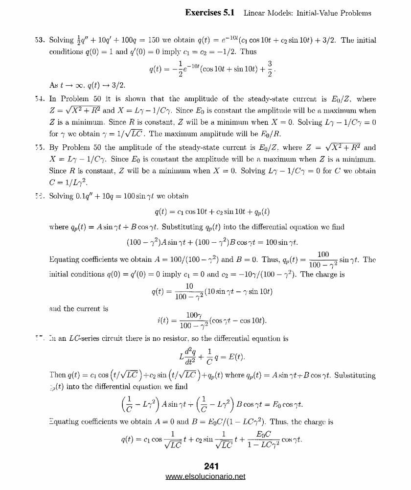
Exercises 5.1 Linear Models: Initial-Value Problems
3. Solving j q" + 10q' -(-100$ = 150 we obtain q(t) = e 10i(ci cos lOt + C2sin 101) + 3/2. The initial
conditions g(0) = 1 and q'(0) = 0 imply f'i — c2 = —1/2. Thus
q(t) = — e_uv(cos 101 + sin lOi) + ^ .
As t —> oc. q(t) —> 3/2.
4. In Problem 50 it is shown that the amplitude of the steady-state current is Eq/Z , where
Z = \J X 2 + R? and X = L j — 1 /C 7 . Since Eq is constant the amplitude will be a. maximum when
Z is a minimum. Since R. is constant. Z will be a minimum when X - 0. Solving £7 — I/C 7 = 0
for 7 we obtain 7 = l/V L C . The maximum amplitude will be Eq/R..
5. By Problem 50 the amplitude of the steady-state current is Eq/Z. where Z = V X2 + R2 and
X = £7 — I/C 7 . Since Eq is constant the amplitude will be a maximum when Z is a minimum.
Since R is constant, Z will be a minimum when X = 0. Solving L7 — l/C '7 = 0 for C we obtain
C = I/L 72.
-j. Solving 0.1 q" + 10q - 100sin7/ wo obtain
g(f) = ci cos lOt + c-2 sin 10< + qp(i)
where qp(t) = A sin yt -i- B cos ~d. Substituting qp(t) into the differential equation we find
(100 — 7'2).-4 sin -it + (100 — y2)B cos = 100 sin -'■/t.
Equating coefficients wc obtain A - 100/(100 —72) and B = 0. Thus, qp(t) = :— sin7t. The.I.UU j'*
initial conditions r/(0) = c/(0) = 0 imply cy = 0 and Co = —10-7/(100 — 7^). The charge is
10q(t) = M ~ Z 2(10sin7i - 7 sin 100
and the current is
= inn00' o(cos 7 - cos 101).1UU — 7"
In an LC-series circuit there is no resistor, so the differential equation is
_ d2q 1 ,
W + c 9 =
Then q(t) = c.\ cos [i,/\JLC ) -j-c2 sin (t/y/LC ) + qp(i) where qp(t) = A sin 7't^-B cos 7t. Substituting
into the differential equation we find
^ - I 72) A sin -r - L-/2 B cos yt = E() cos 71 .
Equating coefficients we obtain A = 0 and B = EqC/(1 — LC72). Thus, the charge is
1 . 1 E qC
www.elsolucionario.net

The initial conditions g(0) — qo and f/(0) = io imply ci — qo — EqC/(1 — LC72) and 0 2 = L
The current is i(t) = q'(t) or
C1 1 * , C2 1 + EqCj .
, ( ) = ~ 7 L c sm7 L S 7 W cos7 I S T = Z c ? sm 7*
1 , 1 { B«C \ . 1 E0C j . ^
= vw Vlc r ■ T icRi rvm *- rrsv “7t5 5. When the circuit is in resonance the form of qp(t) is qp(t) = At cos kt + Bt sin kt where k — 1
Substituting qp(t) into the differential equation we find
q'p + k2(lp = —2kA sin kt + 2kB cos kt = ^ cos kt.
Equating coefficients we obtain 4 = 0 and B = Eo/2kL. The charge is
Eoq(t) = ci cos kt + r,2 sin kt + — — t sin kt.
IkL
The initial conditions g(0) = qo and q'(0) = io imply c\. ~ % and c-2 — U)/k. The current is
Ei(t) = —cik sin kt + 0 2 k cos kt + ——(kt cos kt 4- sin kt)
2/c L
Eq \ Eqgo A') sin kt + io cos kt + — t cos kt.
Exercises 5.1 Linear Models: Initial-Value Problems
2kh 1U J ' 2L
Linear Modelst Bottndary-^Value ProBliKffls!:
1. (a) The general solution is
/ \ . , 2 , 3 , w 0 4■y(x) = ci + c-2x + csx + C4 X + ■
The boundary conditions are y(0) = 0, ;</(0) = 0, y"(L) = 0, y'"(L) = 0. The £:
conditions give c\ = 0 and C2 = 0. The conditions at x — L give the system
2 c3 + 6c4L + ^ j L 2 = 0
r , W() t a6 c 4 + — L = 0.E l
Solving, we obtain C3 — wqL2/ iE I and C4 = —woL/6 E I. The deflection is
y(x) = ^ y ( 6L2x2 - 4Lx3 + .t4).
242www.elsolucionario.net
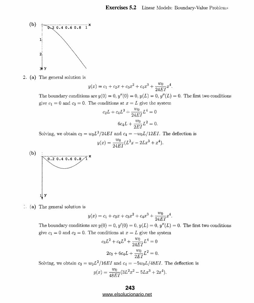
Exercises 5.2 Linear Models: Boundary-Value Problems
(b)0 .4 0 .6 0 .8 1
3? Y
2. (a) The general solution is
, N '•) 'J WQ 4y(x) = ci + c2x + ciyx + c4.x" + —— x .
The boundary conditions are -t/(0) = 0, y"(0) — 0, y(L) — 0, y"(L) = 0. The first two conditions
give ci = 0 and 03 = 0. The conditions at x = L give the system
+ 231714 = 0^ L + l t i L2 = °-
Solving, we obtain C2 = wqL?/24EI and C4 = — w q L /Y2EI. The deflection is
y(x) = ^ j ( L \ .- 2 L X>+x*).
(b)
fa) The general solution is
y(x) = ci+ o2x + c3x2 + C4 X3 -f -
The boundary conditions are y(Q) = 0, y'(0) = 0. y(L) = 0, yf,(L) = 0. The first two conditions
give ci — 0 and c-2 = 0. The conditions at x = L give the system
C«I? + C4 I? + - ^ - L l = 0 24EI
2C3 + 6C4L + ^ - I 2 = 0.2Jbl
Solving, we obtain C3 = w q L 2/ 1 GEl and C4 = —■5u,qL/48£//. The deflection is
*(*) = J | 7 ( 3 lV - 5^ 3 + 2*4)-
243www.elsolucionario.net

Exercises 5.2 Linear Models: Boundary-Value Problems
(b)iTra^ui o ♦ 6 JL-8>1
x
4. (a) The general solution is
/ \ 9 ‘1 wqL 4 . 7Ty(x) = ci + c-ix + c$x- + c4x + — —r sin —x.
£j 1 7T L
The boundary conditions are y(0) = 0, ?/(0) = 0, y(L) = 0, y"(L) = 0. The first two conu
give c.\ — 0 and c? = —wqLs/E Itts. The conditions at x = L give the system
c s L ^ c ^ + ^ L ^ O
2 c 3 + 6 C4 L = 0 .
Solving, we obtain C3 = 3wqL'2 and C4 - — w q L ^ E I^ . The deflection is
WqLy{x)
2EIn*—2L2x + 3Lx2 — x6 4- —
7r ’ — sm —x t t L ,
(c) Using a CAS we find the maximum deflection to be 0.270806 when x = 0.572536.
5. (a) The general solution is
y(x) = ci + C2 X + czx2, + C4<r' 120£JThe boundary conditions are y(0) = 0, y"(0) = 0, y(L) 0, y"(L) = 0. The first two cond:
give cj = 0 and C3 = 0. The conditions at x = L give the system
c 2 L + C 4 I 3 + = 0
6c4i+ i3=a244
www.elsolucionario.net
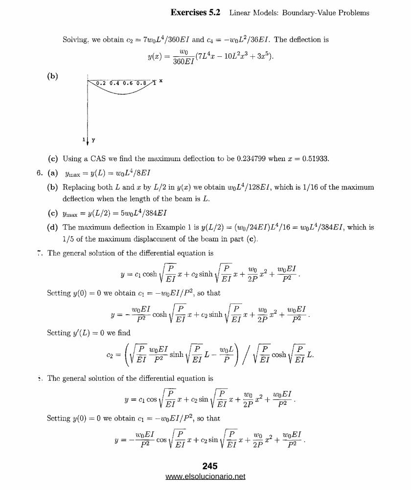
Exercises 5.2 Linear Models: Boundary-Value Problems
Solving, we obtain o> = 7wqL4/360EI and C4 — —wqL2/3QEI. The deflection is
y(x) = — (7L4;r — l()L2;c3 + 3a:0).m E i
(b) . 0 . 2 0 . 4 0 . 6 0 . 8 / 1
*? y
(c) Using a CAS we find the maximum deflection to be 0.234799 when x = 0.51933.
6. (a) '(/max = y{L) = wqLa/8E I
(b) Replacing both L and x by L/2 in y(x) we obtain wqL4/12SEI, which is 1/16 of the maximum
deflection when the length of the beam is L.
(c) ?A„ax = y(L/2) = 5wqL4/3SAEI
(d) The maximum deflection in Example 1 is y(L/2) - {wq/24:EI)L4/16 = wqL'1 /3S4EL which is
1/5 of the maximum displacement of the beam in part (c).
7. The general solution of the differential equation is
/ P . I P wo v wqE Iy = ci cosh V ^ j x + °2 sinh d — x + — x~ + .
Setting y(0) = 0 we obtain c\ = —wqEI/P2, s o that
_ iuqEI x 1 P , ■ x I P , w0 2 , WQE I
W V 571 2 V 57 2P * + p5“Setting y'(L) — 0 we find
_ ( l~P wqE I , i P
02 = 1 ] l % I ^ sh±i E I L - - ^ 1 7 ^ c o s h , / ^ .
w0L ) / f T j P , T ) \iEIC°Sh\'EI
*. The general solution of the differential equation is
Vp , -? '«.'o ■> wo E l y = ci cos y — x + c2 sm ] j ^ j x + ^ p x + ~p 2~ •
Setting y(0) = 0 we obtain c\ = —wqE I/P 2, so that
pp . / P WQ 0 wqE I
y ~ — p2-C0Sv i 7 a: + ':26U1V l 7 :i' + 2P!r + _ p5“ '
245www.elsolucionario.net
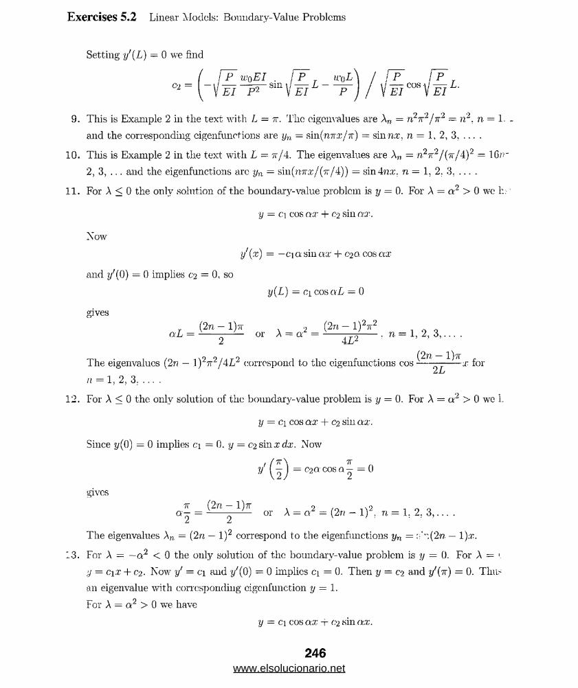
Exercises 5.2 Linear Models: Boundary-Value Problems
Setting y'{L) — 0 we find
, j P w0E I . j P r u\)L\ / / P I P T
C2 = 1 ~p~J /
9. This is Example 2 in the text with L = tt. Tlie eigenvalues are \n = nPn2/*2, = ri2, n = 1. -
and the corresponding eigenfunctions are yn — sin(tt7r;r/7r) = sin nx, n = 1, 2, 3, ... .
10. This is Example 2 in the text with L — tt/4. The eigenvalues are Xn — n27r2/(7r/4)2 ~
2, 3, ... and the eigenfunctions are yn = sin{iittx/ (tt/4)) = sin4n.T. n — 1, 2. 3, ... .
11. For A < 0 the only solution of the boundary-value problem is y = 0. For A = a2 > 0 we h :'
y = ci cos ax + c-2 sin ax.
Now
y'{x) = —ci a sin ax + c2a cos ax
and </(0) = 0 implies ci = 0, so
y(L) = ci cos aL = 0
gives
(2 n — l)?r 2 (2rt — l)27r2a.L = ------- or A = a- = ---— ---. n = 1, 2, 3 ,... .
2 4
The eigenvalues (2n — 1)2tt2/4L2 correspond to the eigenfunctions cos.- -----— for
/i = 1, 2, 3: ... .
12. For A < 0 the only solution of the boundary-value problem is y = 0. For A = a2 > 0 we 1.
y = ci cos ax + c% sin ax.
Since y(0) = 0 implies c\ = 0. y = c2 sm;r dx. Now
/ f ‘K\ t*y ( - 1 = c2a cos a- = 0
gives
* (2 n - i)* or A = q2 = (2„ _ 1)2, „ =Z* z
The eigenvalues A„, = (2n — l)2 correspond to the eigenfunctions yn = :'".(2n — l).r.
13. For A = —a2 < 0 the only solution of the boundary-value problem is y = 0. For A = 1
y = cyx + c-2 - Now y' = ci mid y'(0) = 0 implies ci = 0. Then y — co and y'{n) = 0. Tim-
an eigenvalue with conesponding eigenfunction y = 1.
For A = a2 > 0 we have
y — ci cos ax -f o2 sin ax.
246www.elsolucionario.net
Exercises 5.2 Linear Models: Boundary-Value Problems
Now
;{/(&•) = —CiO: sin ax + c-2 a cos ax
and y'(0) = 0 implies c-2 = 0, so
y'(n) = — ci a sin cwr = 0
gives
an = Tin or A = a2 = n2. n = 1, 2, 3 ,... .
The eigenvalues n? correspond to the eigenfunctions cos nx for n — 0. 1. 2........
For A < 0 the only solution of the boundary-value problem is y = 0. tor A = o:2 > 0 we have
y = ci cos ax + oi sin ax.
Now t/(—tt) = y(n) = 0 implies
ci cos an — Co sin air = 0
(1)Ci cos an + c-2 sin an = 0.
This homogeneous system will have a nontrivial solution when
cos an — sin an
cos an sin an— 2 sin an cos an = sin 2att = 0.
Then2
2an = nn or A = a?" = — ; n = 1. 2. 3, ... .4
When n = 2k — 1 is odd, the eigenvalues arc (2/,; — l)2/4. Since cos(2k — l)n/2 = 0 and
'in(2k — l)n/2 ^ 0. we sec from either equation in (1) that C2 — 0. Thus, the eigenfunctions
orresponding to the eigenvalues (2k — l)2/4 are y = cos(2k — l)x/2 for A: = 1. 2, 3, ... . Similarly,
-.vhen n = 2k is even, the eigenvalues are A:2 with corresponding eigenfunctions y = sin kx for
v = l, 2, 3 , . . . .
The auxiliary equation has solutions
m = i (-2 ± \Ji — 4(A + 1)^ = -1 ± q:.
For A = —a’2 < 0 we have
y = a~x (ci cosh ax -1- q sinh a:c).
The boundary conditions imply
y(0) = ci = 0
y(5) = C2 e~° sinh 5a = 0
- c,\ = c-2 = 0 and the only solution of the boundarv-value problem is y = 0.
247www.elsolucionario.net

Exercises 5.2 Linear Models: Boundary-Value Problems
7 A = 0 we have
y = c\e~x + C2 xe~x
-:-d the only solution of the boundary-value problem is y = 0.
7 . A = «2 > 0 we have
y = e~x (ci cos aa: + 02 sin cm : ) .
X i/(0) = 0 implies c\ = 0, so
y( 5) = C2e-5 sin 5oi = 0
772 7T25a = nn or A = a2 = “ , n = 1 .2 ,3 ,... .
Zo9 2
— T n~7T* r _r . U7Ti ::e eigenvalues An = correspond to tlic cigcnfunctions yn = e " sin — x tor n = 1, 2.
25 ' 51-; . A < —1 the only solution of the boundary-value problem is y = 0. For A = — 1 v-
. — c\X + c2. Now y' — ci and ?/(0) = 0 implies ci = 0. Then y = c2 and y'( 1) = 0. Thus, ,• -
an eigenvalue with corresponding eigenfunction y = 1.
T'.r A > —1 or A + 1 = a2 > 0 we have
y = ci cos (xx + c-2 sin ax.
Xow
y1 — —cio: sin ax + c2a cos ax
</(0) = 0 implies 0 2 = 0. so
y'(l) = —cia sin a = 0
V'r'S
a = nn, A + 1 = a2 = n2n2, or A = n2n2 — 1, n = 1,2 ,3 ,... .
eigenvalues n2n2 — 1 correspond to the eigenfunctions cosnirx for n — 0, 1, 2, ... .
1”. I- A = q2 > 0 a general solution of the given differential equation is
y = c\ cos(ct In ai) + C2sin(alna:).
rir.ce In i = 0, the boundary condition y( 1) = 0 implies c.\ = 0. Therefore
y = c2 sin(a In x).
V'ing In cJ = n wc find that y (e*) = 0 implies
c2 sin «7r = 0
:: = Tin, n — 1, 2. 3, ... . The eigenvalues and cigcnfunctions are, in turn,
9 9A = a" = 7T, n = l ,2 ,3 , . . . and y — sin(nlna;).
248www.elsolucionario.net

Exercises 5.2 Linear Models: Boundary-Value Problems
For A < 0 the only solution of the boundary-value problem is y = 0.
18. For A = 0 the general solution is y = c\ + c2 lna;. Now y' = c^fx, so y'(e~l ) = c2e = 0 implies
C-2 = 0. Then y = c\ and y(l) = 0 gives c\ = 0. Thus y(x) = 0.
For A = —a2 < 0. y = c\x~a + c2xa. The boundary conditions give co = c\,e2a and c\ = 0. so that
C2 = 0 and y(x) = 0.
For A — a2 > 0. y = c\ cos (a In x) + C'2sm(alii.r). From y(l) = 0 we obtain c\ = 0 and y =
co sin(o: In.?;). Now 1/ = C2.{a/x) cos(et lna;). so y'(e~l) = o2ea cos a = 0 implies cos a — 0 or
a = (2n — 1)tt/2 and A = a2 = (2n — l)2n2/4 for n = 1, 2. 3. ... . The corresponding eigenfunctions
arc• ( 2n ~ 1 1yn = sm ( — -— ix lna; J .
19. For A = of1. a: > 0, the general solution of the boundary-value problem
y(4) - Ay = 0. y(0) = 0, / (0 ) = 0, y(l) = 0, y"(l) = 0
is
y = C] cos ax + 02 sin ax 4- (‘‘i cosh ax + <74 sinh ax.
The boundary conditions y(0) - 0, y"(0) = 0 give ci + C3 = 0 and — c.\a2 + c$a2 = 0, from which
we conclude ci = C3 = 0. Thus, y = C2sina;r + 04 sinh ora. The boundary conditions y( 1) = 0.
yir( l) = 0 then give
C2 sin a + C4 sinh a = 0
ey—coa sin a + cja sinh a = 0.
In order to have nonzero solutions of this system, we must have the determinant of the coefficients
equal zero, that is,
sin a- sinh a
-a2 sin a a 2 sinh a
But since a > 0, the only wav that this is satisfied is to have sin a- = 0 or a = nn. The system
is then satisfied by choosing 0 2 7 0, C4 = 0, and a — nn. The eigenvalues and corresponding
eigenfunctions are then
An = O'* = (twt)'1, n = 1,2. 3 ,... and y — sin nnx.
- . For A = a4, a > 0, the general solution of the differential equation is
y = ci cos ax + c2 sin ax + C3 cosh ax + 0 4 sinh ax.
The boundary conditions y'(0) = 0. y'"(0) = 0 give + c a. = 0 and —c2a3 + C4C/ = 0 from which
we conclude C2 = c.\ = 0. Thus, y = ci cos ax + C3 cosh cm;. The boundary conditions y(n) ~ 0,
= 0 or 2 a2 sinh a sin a = 0.
249www.elsolucionario.net
Exercises 5.2 Linear Models: Boundary-Value Problems
'/''(tt) = 0 then give
C2 COS Q7T + C4 cosh G:7T = 0
0 9—Cq\ COS Q'TT + Cl A cosh Q:7T = 0.
The determinant of the coefficients is 2a2 cosh a cos a = 0. But since a > 0. the only way
:his is satisfied is to have cos an = 0 or a = (2n — l)/2, n = 1, 2, 3. ... . The eigenvalues :.
corresponding eigenfunctions are
. 4 (2n — 1\4 , f2 n —\\Xn = a = I — -— J . n = 1,2,3.... and y — cos I — -— J x.
21. If restraints are put on the column at = L/4. x = L/2, and x = 3L/4, then the critical
load will be P4.
(a) The general solution of the differential equation is
I p j p
y = ci cos yj-£jx + c‘2 sin \j -gj x + S.
Since the column is embedded at x — 0. the boundary conditions arc y(0) = j/(0) = 0. If <
this implies that ci = C2 = 0 and y(x) = 0. That is, there is no dcflcction.
i b) If S 0, the boundary conditions give, in turn, ci = —5 and C2 = 0. Then
I py = d I 1 - cos y — x I .
In order to satisfy the boundary condition y(L) = S we must have
FT \ FTd = i | l- coey — I or cosy— L = 0.
Tliis gives J P /E IL = utt/2 for n = 1. 2, 3, ... . The smallest value of Pn. the Euler loai
then ___
!P\ T ir „ 1 fir2EI\V E l ~ 2 °r 1 “ 4 ( L2 j '23. I: A = a2 = P /E I. then the solution of the differential equation is
y = ci cos ax + C2 sin a® -1- c$x + c4.
250www.elsolucionario.net

Exercises 5.2 Linear Models: Boundary-Value Problems
The conditions y(0) = 0, y"(0) - 0 yield, in turn. c\ -j- c,\ — 0 and c\ = 0. With c\ = 0 and c4 = 0
the solution is y = c2 sin am + c&x. The conditions y(L) = 0, y"(L) = 0. then yield
C2 sin aL + c^L = 0 and c2 sin aL = 0.
Hence, nontrivial solutions of the problem exist only if sin aL = 0. From this point on, the analysis
is the same as in Example 3 in the text.
(a) The boundary-value problem is
0 + A 0 - O , y(0) = 0,s/'(0) = 0, y(L) = 0,y'(L) = 0,
where A = a2 = P /E I. The solution of the differential equation is y = c\ cos am + c2 sin ax +
c-iX + C4 and tlie conditions y(0) - 0. y"(0) = 0 yield c\ — 0 and c.4 = 0. Next, by applying
y(L) — 0, y\L) = 0 to y = co sin ax + c%z we get the system of equations
0 2 sin aL + c^L = 0
ac2 cos aL +■ eg = 0.
To obtain nontrivial solutions 0 2 , 03, we must have the determinant of the coefficients equal to
zero:sin aL L
= 0 or tan 3 = .0,a cos aL 1
where 8 = aL. If 8 n denotes the positive roots of the last equation, then the eigenvalues are
found from 3n = anL = \fKh L or \n = (.8 n/L )2. From A = P /E I we see that the critical loads
are Pn = d^E I/L2. With the aid of a CAS we find that the first positive root of tan 8 ~ ,[3
is (approximately) 8 1 = 4.4934, and so the Euler load is (approximately) P\ •= 20.1907E lf I?.
Finally, if we use C;s = —c.0.a cos aL . then the deflection curves are
yn(x) - c2 sina„,r + c$x = c2 sm'Pn
-x'0n '
— COS p n j X
(b) With L = 1 and c2 appropriately chosen, the general shape of the first buckling mode,
'4.4934?yi(;r) = c2
4.4934 sm I — -— x cos(4.4934)} x
is shown below.yi
0.4The general solution is
IPy = c:i cos y — ux c>2 sin */= ux.
V t '
251www.elsolucionario.net
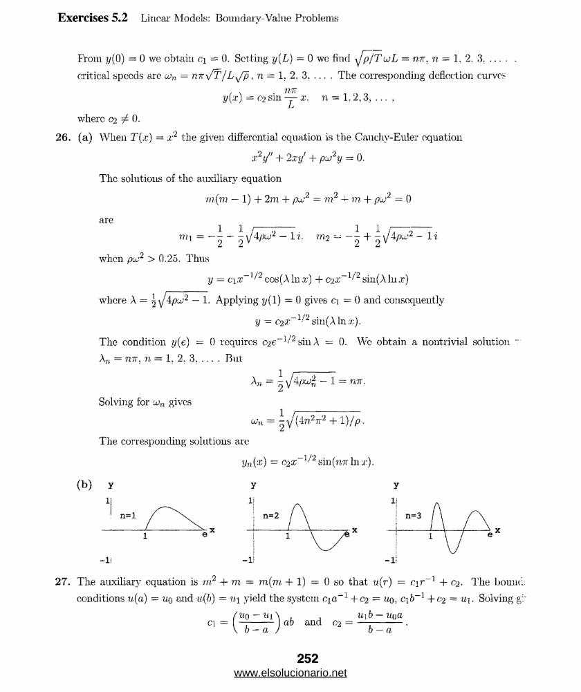
Exercises 5.2 Linear Models: Boundary-Value Problems
From ;i/(0) = 0 we obtain c,\ = 0. Setting y(L) = 0 we find \[p(TuL = mr, n — 1, 2. 3. ... .
critical speeds arc Co1-/}. — ??.7T yT j L^fp, n = 1. 2. 3. ... . The corresponding dcflection curves
" c-2 sin ~ x, n — 1.2,3, ... ,
where C2 ^ 0.
26. (a) When T(x) = x1 the given differential equation is the Cauchy-Euler equation
x2y" + 2xy' + p J2y z 0.
The solutions of the auxiliary equation
rnfjn — 1) + 2 m + pJ2 = m2 -r in + p:J 2 = 0
are
mi = - - - - sjApuS2 - 1 i. rn2 - - - + - \/ApJ2 - 1 i
when p'J2 > 0.25. Thus
y = ci a; 1/2 cos (A In x) + c2x 1/2 sin(Aln.r)
where A - \^Ap,jj‘2 — 1. Applying y( 1) = 0 gives ci = 0 and consequently
y — C2X-1/2sin(Alnx-).
The condition y(e) — 0 requires C2e~1'/2sinA = 0. Wc obtain a nontrivial solution “
An = mr, n = 1, 2, 3, ... . But
Solving for ion gives
= W (4n27T2 + 1 )/p .
The corresponding solutions are
V n { x ) = 0 2 X~]’2 sui(mr In a:).
-l!
27. The auxiliary equation is m2 + m = m(m + 1) = 0 so that u(r) - c:\r 1 + c-2- The bound:
conditions it (a) = uq and u(b) ~ u\ yield the system cic"1 +C2 - uq, cife-1 + 0 2 = u\. Solving g:_
'UQ-Uy\ u\b — uq(ici = 1 —---- ab and C2 :
b — a b — a
252www.elsolucionario.net

Exercises 5.2 Linear Models: Boundary-Value Problems
Thus/«o - «i\ ab Uib-UQO.u(r) = —--- — + —:---- •V b — a J r b — a
2 S. The auxiliary equation is rrr = 0 so that u(r) - ■ + C2I11 r. The boundary conditions u(a) — uq
and u(b) — ui yield the system ci -I- C2 In a = «o, ci + 02 In b = «i. Solving gives
1/1 111 a — Uq 111 b Uq — U,i
CI = — k(V 6j— “ad C 2 = h^/io-
Thus. . Ui In a — u-o hi b 1/0 — u-\ . u.q ln(r/6) — «i ln(r/a)
“ (r) = M a / i ) + W i , ) h ‘ r = -------------------- '
-It. The solution of the initial-value problem
x" H- U2x = 0; .t(0) = 0, x'(Q) = vo, co2 = 10/m
is x(t) — (vo/uj)smuit. To satisfy the additional boundary condition .7.(1) = 0 we require that
u — ni\, n — 1. 2. 3, ... . The eigenvalues A = u;2 — n2TT2 and eigenfunetioris of tlie problem
arc then x(t) = (vu/nir) smnnt. Using J 2 — 10/m we find that the only masses that can pass
through the equilibrium position at t = 1 me m„. = 10/yr?r2. Note for n 1, the heaviest mass
mi = 10/tt2 will not pass through the equilibrium position 011 the interval 0 < t < 1 (the period
of x(t) = (vo/tt) sin Tit is T = 2. so 011 0 < t < 1 its graph passes through ;*■ = 0 only at i = 0 and
f = l). Whereas for n > l. masses of lighter weight will pass through the equilibrium position n — l
times prior to passing through at t = l. For example, if n = 2. the period of x(t) = (vq/2ir) sin2-7r/;
is 2tt/2tt — 1. the mass will pass through x = 0 only once (t = | ) prior to t = 1; if n = 3. the
period of x(L) = (t’o/37r) sin37rt is | , the mass will pass through x = 0 twice (t = ?5 and t = |)
prior to t = 1: and so on.
I ". The initial-value problem is
x" + —x! + —x = 0, .rfO) = 0. a/(0) = ■(.?(>. m rn
With k = 10. the auxiliary equation has roots 7 = — 1/mzk \/l — 10m/m. Consider the three cases:
(i) rn = -pj. The roots arc 71 = 72 = 10 and the solution of the differential equation is
x(t) = The initial conditions imply ci — 0 and C2 = (’0 and so x(t) = uote”10*.
The condition x(l) = 0 implies t'ofi-10 = 0 which is impossible because t'o 7= 0.
ii) 1 — 10??? > 0 or 0 < rn < ^ . Tlic roots arc
1 \ ________ \ 1 ________"7i = ------ V l — 10 m and 72 = ----1-- V l — 10m
rn rn rn rn
and the solution of the differential equation is x(t) = c.ie7lt — C2 C72t. The initial conditions imply
Ci + C2 = 0
0 l c l + l2 c2 = t - 'o
253www.elsolucionario.net

Exercises 5.2 Linear Models: Boundary-Value Problems
so Cl = t'o/ (71 - 7-2); C2 = - t’o/(71 - 72), and
x-(t) = — —— (e'llt - e^1).71 - 72
Again, x(l) = 0 is impossible because vo ^0 .
(Hi) 1 — 10m < 0 or m > . The roots of the auxiliary equation are
71 = — —---— \/10m — 1 i and 'v? —----1- — \f 10m — 1 im rn m m
and the solution of the differential equation is
x(t) = c\e~ m cos — x/lOm — I t + 0 )e~f'!m sin — \/l0m — It. m " m
The initial conditions imply Ci = 0 and C2 = mvo/ y/lQm — 1, so that
x(t) = e~t/msin ( — y/lOrn — 1A .v J y/lQm - 1 \m )
The condition .t(1) = 0 implies
rnVQ
y/10m - 1 m
1
2 sin— y/\Qm — 1 — 0
sin — \/l0m — 1 = 0771— y/ 10m — 1 = T17T m
10m — 1--- ~— = n tt . 7i = 1,2.3,. ..7nz
(n"n )m “ — 10m -*-1 = 0
10V100 - 4ri27r2 5 ± \/25 — n?n2 m = ----= ----- 2 ----•
2 n Z7T- 71 7T
Since m is real. 25 — n2n2 > 0. If 25 — a2tv2 = 0; then n2 = 25/tt2, and n is not an integei .
25 — n27T2 = (5 — ri7r)(5 + 7 11r) > 0 and sincc n > 0. 5 + nn > 0. so 5 — nn > 0 also. Then n <
and so n = 1. Therefore, the mass m will pass through the equilibrium position when t — 1 :
5 + V25 - n2 , 5 - V25-7T2mi = ----- ---- and m29 9
TT" TT
31. (a) The general solution of the differential equation is y = c\ cos 4a:+02 sin Ax. Prom yo — y{\
we see that y = yo cos Ax + 0 2 sin Ax. From yi — y(7t/2) = yo we see that any solutioi.
satisfy yo — Vi- We also see that when yo = yi, y = yocosAx + c2sin4;c is a solution
boundary-value problem for any choice of 0 2 . Thus, the boundary-value problem docs no-
a unique solution for any choice of yo and y\.
(b) Whenever yo = y\ there are infinitely many solutions.
254www.elsolucionario.net

Exercises 5.2 Linear Models: Boundary-Value Problems
(c) When ijq / y\ there will be no solutions.
(d) The boundary-value problem will have the trivial solution when yo = yi = 0. This solution
will not be unique.
'.2. (a) The general solution of the differential equation is y — C] cos4r + C2sin4.T. From 1 = ;y(0) = c\
we see that y = cos4:r + C2sin4;r. From 1 = y(L) = cos 4L + 0 2 sin4L we sec that
C2 = (1 — cos4L)/ sin 4L. Thus,
will be a unique solution when sin 4L 7 0; that is, when L ^ A’tt/4 where A: = 1, 2, 3, ... .
(b) There will be infinitely many solutions when sin4L = 0 and 1 — cos 4L — 0; that is, when
L = &7t/2 where k = 1, 2, 3, ... .
(c) There will be no solution when sin4L 7 0 and 1 — cos4L 7 0; that is, when L = kn/4 where
: d) There can be 110 trivial solution since it would fail to satisfy the boundary conditions.
M ! a) A solution curve has the same ^-coordinate at both ends of the interval [—tt, tt] and the tangent
lines at the endpoints of the interval are parallel.
b) For A = 0 the solution of y" = 0 is y = cix + c% From the first boundary condition we have
or 2citt = 0. Thus, ci = 0 and y = 0 2 - This constant solution is seen to satisfy the boundary-
value problem.
For A = —a? < 0 we have y = c\ cosh ax + 0 2 sinh ax. In this case the first boundary condition
gives
or 2c‘2 sinh ott = 0. Thus C2 = 0 and y = c\ cosh ax. The second boundary condition implies in
a similar fashion that c\ = 0. Thus, for A < 0. the only solution of the boundarv-value problem
is y = 0.
For A = a2 > 0 we have y = c\ cosax + casinos. The first boundary condition implies
y(-7r) = C'lTT + c2 = t/(? r) = Ci-n - c2
y(—tt) = ci cosh(—a7r) + C2sinh(—air)
= ci cosh air — c<2 sinh ottt
= y('n) = ci cosh cv7T 4- c-2 sinh air
y(—tt) = ci cos(—c*7r) + C2 sin(—a7r)
= C\ COS tt7T — C‘2 S in Q7T
y(ir) — ci cos air + C2 sin a%
255www.elsolucionario.net
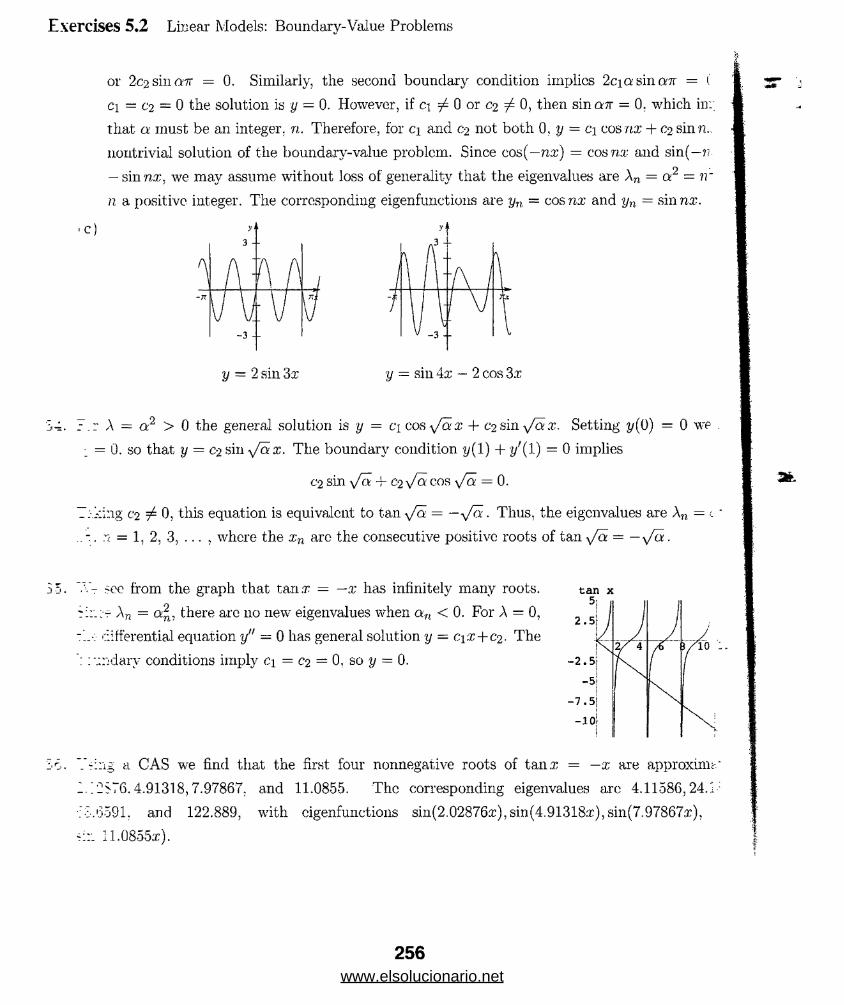
Exercises 5.2 Linear Models: Boundary-Value Problems
or 2c2sinmr = 0. Similarly, the second boundary condition implies 2c.ia sin an = (
a — C2 = 0 the solution is y — 0. However, if ci ^ 0 or C2 / 0, then sinaTr = 0, which in:;
that a must be an integer, n. Therefore, for ci and (>2 not both 0, y = c\ cos nx + 0 2 sinn.,
nontrivial solution of the boundary-value problem. Since cos(—nx) = cos nx and sin(—?;
— sin nx, we may assume without loss of generality that the eigenvalues are Xn = a2 — n~
n a positive integer. The corresponding eigenfunctions are yn = cos nx and yn = sin nx.
■ c
y = 2 sin 3x’ y = sin 4a; - 2 cos Sx
34. A = a2 > 0 the general solution is y = ci cosy/ax + C2 sin /tvx. Setting y(0) = 0 we .
: = 0. so that y = c-j sin y/ax. The boundary condition y(l) + y'( 1) = 0 implies
C2 sin y/a -f C2 y/a cos y/a = 0.
7:-.king t'2 ^ 0, this equation is equivalent to tan y/a = —y/a. Thus, the eigenvalues are An =
r( = 1, 2, 3, ... , where the xn are the consecutive positive roots of tan y/a = —y/a.
35. ’.Vt sec from the graph that tanx = —x has infinitely many roots.
r An = a2, there arc no new eigenvalues when an < 0. For A = 0,
differential equation y" = 0 has general solution y — C\x+C2 - The
: : \;ndary conditions imply c\ = C2 = 0, so y = 0.
So. Vring a CAS we find that the first four nonnegative roots of tana; = —x are approxinic-.'
1.! 2576.4.91318,7.97867. and 11.0855. The corresponding eigenvalues arc 4.11586,24.1:
: S.'3591. and 122.889, with cigenfunctions sin(2.02876:r)5 sin(4.91318.'E), sin(7.97867;r).
*::: 11.0855a;).
tan x
256www.elsolucionario.net

Exercises 5.2 Linear- Models: Boundary-Value Problem.'
In the case wlien A = — a2 < 0. the solution of the differential
-::uation is y = c\ cosh ax 4- co sinh ax. The condition y(0) - 0
;ives ci = 0. The condition y(l) — J>(/(1) = 0 applied to
. = c-2 sinh ax gives C2(sinh a — |a: cosh a) = 0 or tanh a = ^a. As
::-.n be seen from the figure, the graphs of y — tanh a: and y - in-
irvscct at a single point with approximate x-coordinate a i = 1.915.
7'r.us, there is a single negative eigenvalue Ai = —af ~ —3.667 and
'I:-- corresponding eigenfuntion is y\ = sinh 1.915.x.
r :r A = 0 the only solution of the boundary-value problem is y = 0.
A = q2 > 0 the solution of the differential equation is y - c\ cos ax 4- c-2 sin ax. The condi:
. 0 = 0 gives ci = 0, so y = C2 sin ax. The condition y(l) — i/(l) = 0 gives C2(sin a —^a cos a =
- • the eigenvalues are An — a 2 when an, n = 2, 3. 4. . . . , are the positive roots of tan« = ^Q. I ’?
- CAS wc find that the first three values of a are a2 - 4.27487. 0:3 = 7.59655, and a4 = 10.SI
TI.e first three eigenvalues are then A2 = a^ = 18.2738, A3 = q| = 57.7075, and A4 = a2 = 116.
—i"Ii corresponding eigenfunctions yi = sin 4.27487a;. ys = sin 7.59655a;, and 2/4 = sin 10.8127.".
7.:' A = a4, a > 0; the solution of the differential equation is
y = ci cos cvx + C2 sin ax + C3 cosh ax 4- c4 sinh ax.
T_t boundary conditions y(0) = 0. y'(0) = 0; y( 1) = 0. yf( 1) = 0
in turn,
ci + C3 = 0
a (>2 4 0 0 4 = 0,
ci cos a 4 0 2 sin a 4 C3 cosh a: + c4 sinh a = 0
—Ci a sin a 4 oioc cos a 4 c%a sinh a- + c,ta: cosh a = 0.
T I . t first two equations enable us to write
ci (cos a — cosh a) 4- C2(sin a — sinh a) = 0
ci(— shift — sinh a) 4 C2(cos a — cosh a) = 0.
determinant| cos a — cosh a sin a — sinh a
| — sin a — sinh a cos a — cosh a j
:_.::Iifies to cos a cosh a = 1. From the figure showing the graphs of 1/ cosh a: and cosx. --
= 0
257www.elsolucionario.net

that this equation has an infinite number of positive roots. With the aid of a CAS the first, for..
arc found to be ai = 4.73004, CV2 = 7.8532, 0:3 — 10.9956, and 0.-4 = 14.1372. and the oorres,:
eigenvalues arc Ai = 500.5636, A2 = 3803.5281, A3 = 14,617.5885, and A.i = 39,944.1890. IV .
third equation in the system to eliminate 02, we find that the eigenfunctions arc
yn — {—sinavt + sinh an)(cos anx — coshanx) + (cosan — cosh an)(sin anx — sinh a,,.
Exercises 5.2 Linear Models: Boundary-Value Problems
Nonlinear Models
1. Tlie period corresponding to z(0) = 1. x'(Q) = 1 is approxi
mately 5.6. The period corresponding to .i'(0) = 1/2. a/(0) = — 1
:=■ approximately 6.2.
2. llic solutions are not periodic.10f
5;
f i . 1 0 . 2 0 . j
The period corresponding to ;.r(0) = 1. ay(0) = 1 is approx
imately 5.8. The second initial-value problem does not have
h periodic solution.
258www.elsolucionario.net
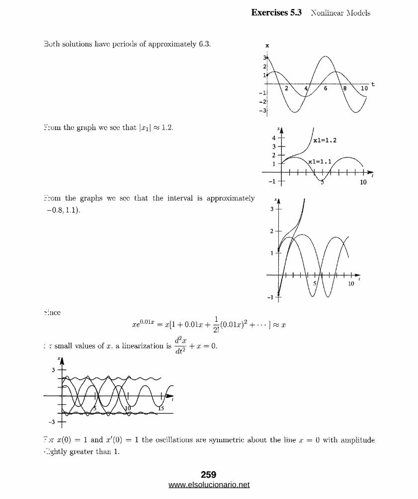
Exercises 5.3 Nonlinear Models
joth solutions have periods of approximately G.3.
From the graph we see that |j i | ~ 1.2.
rrorn the graphs we sec that the interval is approximately
-0.8.1.1).
nice
xe0,°ix = x[l + 0.01a; + ^y(O.Olx)2 +
d?xr small values of x. a linearization is — + x = 0.
a t /
1x
:>r :i’(0) = 1 and 3 (0) = 1 the oscillations are .symmetric about the line x = 0 with amplitude
ightly greater than 1.
259www.elsolucionario.net
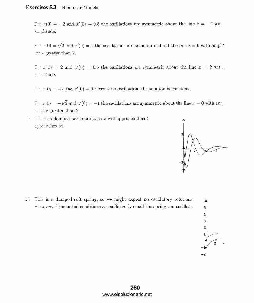
7 : r .r(0) = —2 and a/(0) --- 0.5 the oscillations are symmetric about the line x — —2 wir.
-.:.:piitude.
7 .r 0) = and a/(0) = 1 the oscillations are symmetric about the line x = 0 with amp.
greater than 2.
r - r .O .) = 2 and ;r'(0) = 0 .5 the oscillations are symmetric about the line x = 2 wit',
r/.itude.
7 : (j) = —2 and ay(0) = 0 there is no oscillation; the solution is constant.
7 : r 0) = — V2 and x'(0) — —1 t.lie oscillations arc symmetric about the line x = 0 with an.
l::tle greater than 2.
T‘:i' is a damped hard spring, so x will approach 0 as t x
.v: "roaches oo.
Exercises 5.3 Nonlinear Models
I I . . /.is is a. damped soft, spring, so we might expect no oscillatory solutions. x
. v.-ever. if the initial conditions are sufficiently small the spring can oscillate. 5:
7
-2
www.elsolucionario.net
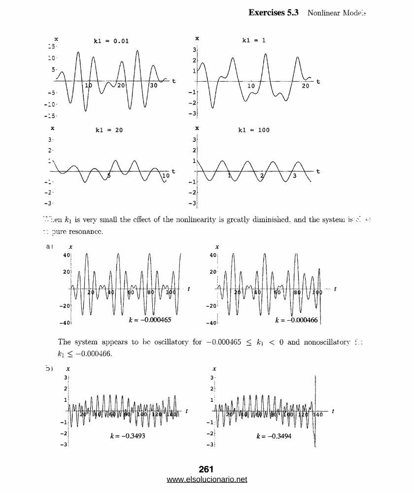
Exercises 5.3 Nonlinear Model?
kl = 0.01 kl = 1
kl = 20
j-
2 -
10
'•VV.en k\ is very small the cffect of the nonlinearity is greatly diminished, and the system is
:: pure resonance.
ai x
The system appears to ho oscillatory for —0.000465 < ky < 0 and nonoseillatory
< -0.000466.
o>
261www.elsolucionario.net

Exercises 5.3 Nonlinear Models
The system appears to be oscillatory for —0.3493 < k\ < 0 and nonoscillatory for A"i < -
.3. For A2 — a-'2 > 0 we choose A = 2 and u; = 1 with ,r(0) = 1
;-::d 1r/(0) = 2. For X2— j2 < 0 we choose A = 1/3 and uj = 1
~'ith x(0) = —2 and x'(0) = 4. In both eases the motion
'..rresponds to the ovcrdainped and underdamped cases for
~: 'ling/mass systems.
.4. a) Setting dy/dl = v. the differential equation in (13) becomes d,v/dt - —gR2/y2. But
chain rule, dv/dt = (dv / dy)(dy / dt) = v dv/dt. so vdv/dy = —gR?/y2. Separating •
and integrating we obtain
,2 dv ...., i ,2 _ yti1v dv — — o/?w —k- and -v = :--- r c.
V 2 y
Setting v = vq and y = R we find c = —gR + j t ’o and
f>2v2 = 2g— - 2gR + vjj.
b ) As y —> co we assume that, v —»0+. Then t’o “ 2gR and ?,’o : y/2gR.
< c ) Using g = 32 ft/s and R = 4000(5280) ft we find
t'0 = ^2(32) (4000) (5280) « 36765.2 ft/s « 25067 mi/hr.
d) c{) = ^/2(0.165)(32)(1080) « 7760 ft/s « 5291 mi/hr
:a) Intuitively, one might expect that only half of a 10-pound chain could be lifted by a
vertical force.
■ b ) Since x - 0 when t = 0. and v = dx/dt = yTOO — 64;r/3, we have u(0) = \/l60 ~ 12.L
■ c) Since x should always be positive, we solve x(t) = 0, getting t = 0 and t = f y'5/2 *
Since the graph of x(t) is a parabola, the maximum value occurs at trn = |y/5/2. (~
also be obtained by solving xr(t) = 0.) At this time the height of the chain is x(t):
ft. This is higher than predicted becausc of the momentum generated by the force. Y\
chain is 5 feet high it. still has a positive velocity of about. 7.3 ft/s, which keeps it goin
for a while.
• d ) As discussed in the solution to part (c) of this problem, the chain has momentum g-
by the force applied to it that will cause it. to go higher than expected. It will then :
to below the expected maximum height, again due to momentum. This, in turn, will
to next go higher than expected, and so on.
www.elsolucionario.net

Exercises 5.3
(a) Setting dx/dt = v. the differential equation becomes (L — x)dvjdt — v~ - Lg. But. by the
Chain Rule, dv/dt = (dv/dx) (dx/dt) = vdv/dx, so (L — x)v dv/dx — v2 = Lg. Separating
variables and integrating we obtain
1 1 dv = ---- dx and - ln(i’2 4- Lg) = — ln(L — x) + In c,
v2 + Lg L - x
so \Jv2 + Lg = c/(L — x). When x - 0, v = 0, and c = LyfLg. Solving for v and simplifying
we get
dx _ jL jj$ L x - 3 ? )
dt ~ ~ L - i
Again, separating variables and integrating wc obtain
L - x y/2 Lx - a;2:dx - dt a n d --- ==— = t + c i.
yjLg(2Lx-x2) ......... VLg
Since ;r(0) = 0. we have = 0 and \/2Lx — x2/ \fLig = t. Solving for x we get
dt \/L - gt2x(t) = L — \JL"2 — Lgt'2 and v(t) = -77 = - •
b) The chain will, be completely on the ground when x(t) = L or /; = y L /g .
(c) The predicted velocity of the upper end of the chain when it hits the ground is infinity,
(a) Let (x,y) be the coordinates of S2 on the curve CJ. The slope at (x.y) is then
dy/dx = (i'i t - y)/( 0 - x) = (y - vi i)/x or xy' - y = -vtf.
ib) Differentiating with respect to a; and using r = t’i/ t ’2 gives
1 1 1 1 dtxy +y - y = - t ’i -7 -
dx
„ dt dsxy ■ — t1! — —
ds d.x
- (- V i + W )V-2
xy" = r\j 1 + (yf)2.
263www.elsolucionario.net
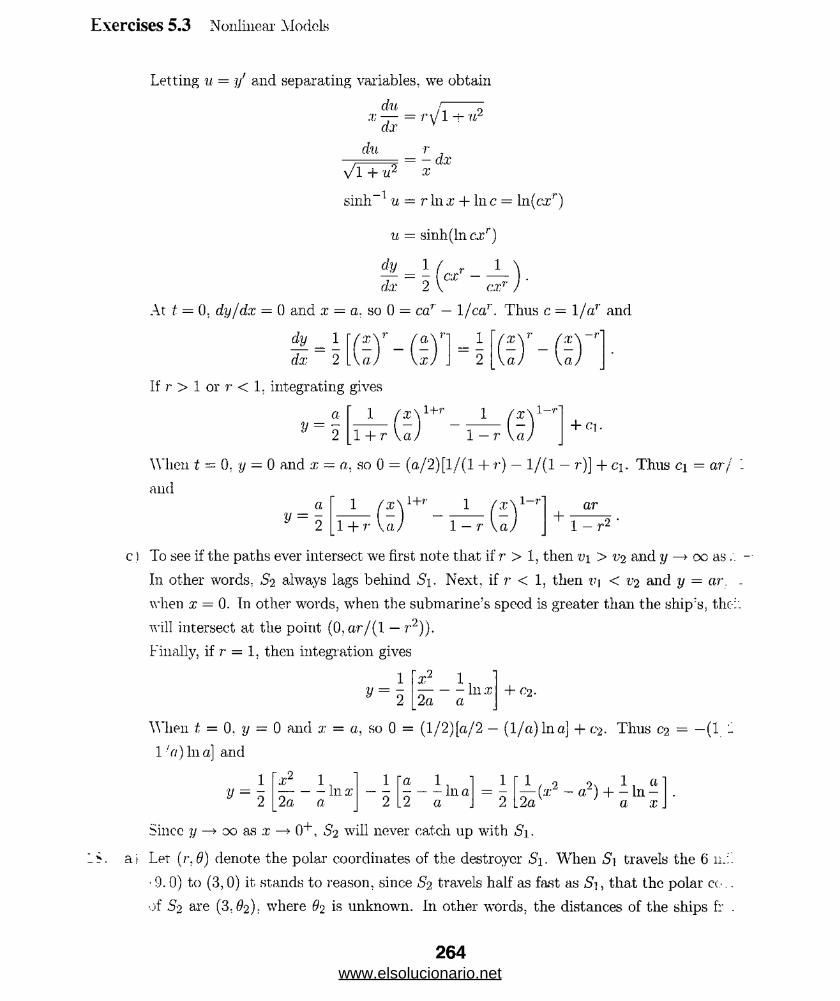
Exercises 5.3 Nonlinear Models
Letting u = ?/ and separating variables, we obtain
du
dx
du r 2 = r y l ^ 2
du r
7 T + 7 = ;
sinh-1 u — r In x + Inc = ln(c.r')
u = sinh(ln cxr)
dy 1 / _ 1
At t = 0. dy/dx = 0 and x = a. so 0 = car — 1 jcar. Thus c = 1/7/ and
dy
dx- )' - ( “-a j \x
If r > 1 or r < 1. integrating gives
1 + r \aj
X\1+r
1 — r
1—r'+ Cl.
When t = 0, y = 0 and x = a, so 0 = (a/2)[1/(1 + r) — 1/(1 — 7-)] + c\. Thus ci = arj
and1 x y + , . _ 1
1 - r
1—r+
arr2 ■1 + r V a J
To see if the paths ever intersect we first note that if r > 1, then v\ > v2 and y —> oo as. .
In other words. S? always lags behind Si. Next, if r < 1. then < v2 and y = ar.
when x = 0. In other words, when the submarine’s speed is greater than the ship's, thc-i.
will intersect at the point (0, arj(\ — r2)).
Finally, if r = 1. then integration gives
Vx?
2a■ In x + c2.
When t = 0, y = 0 and x = a, so 0 = (l/2)[a/2 — (1/a) In a] + c2. Thus C2 = —(1 -
1 7/)Inal and
V =1 r*2 1 n 1 1 'a 1 1 '
-----Ill x ----111 a2 a a ~ 2 .2 a “ 2 .t e
2\ . 1 1 a a J H— In — a x
Since y —> oo as x —*• 0+, S2 will never catch up with Sy.
ai Let (>\9) denote the polar coordinates of the destroyer Si. When Si travels the 6 n_;’
■ 9. 0) to (3,0) it stands to reason, since S2 travels half as fast as S i, that the polar co. -
of S~2 axe (3,02); where 02 is unknown. In other words, the distances of the ships fr .
264www.elsolucionario.net
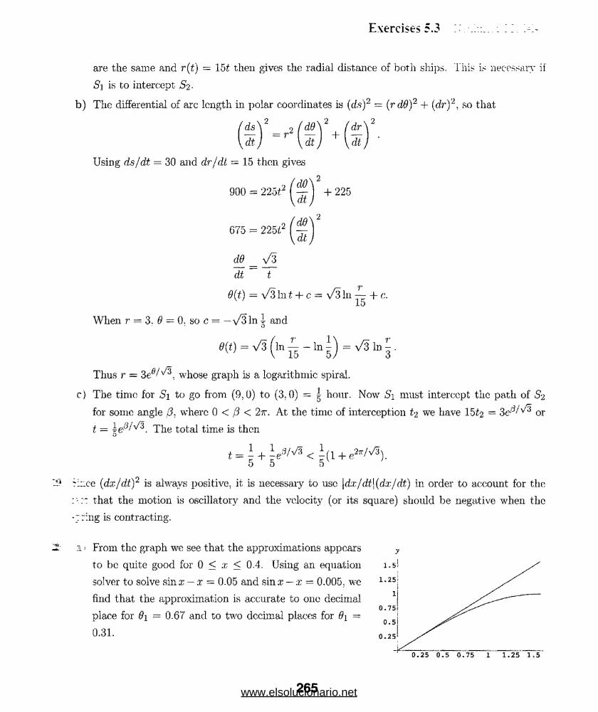
Exercises 5.3
are the same and r(t) = lht then gives the radial distance of both ships. This is necessary ii'
S] is to intercept S-2 -
b) The differential of arc length in polar coordinates is (ds)2 = (rdff)2 + (dr)2, so that
'ds
dt= r~
dd"
dt
Using ds/dt = 30 and dr/dt = 15 then gives
dt
875
de
dt
V3
t
$(t) = V3 In t + c = \/3 In ~ + c.JLO
When r = 3. 0 = 0. so c = — \/31n i and
Thus r = 3 e ^ 3: whose graph is a logarithmic spiral,
c) The time for Si to go from (9,0) to (3.0) = g hour. Now Si must intercept the path of S-2
for some angle Q, where 0 < ,Q < 2ir. At the time of interception to we have 15 2 = 3ed/v '3 or
t = The total time is then
( = I + 1 8/vf< l (1 + (!2,/V5).5 5 5
rir.ee (dx/dt)2 is always positive, it is necessary to use \dx/dt\(dx/dt) in order to account for the
: that the motion is oscillatory and the velocity (or its square) should be negative wrhen the
-Ti'ing is contracting.
From the graph we see that the approximations appears
to be quite good for 0 < x < 0.4. Using an equation
solver to solve sinx — x = 0.05 and sinx — x = 0.005. we
find that the approximation is accurate to one decimal
place for 6\ = 0.67 and to two dccimal places for 6\ —
0.31.
265www.elsolucionario.net
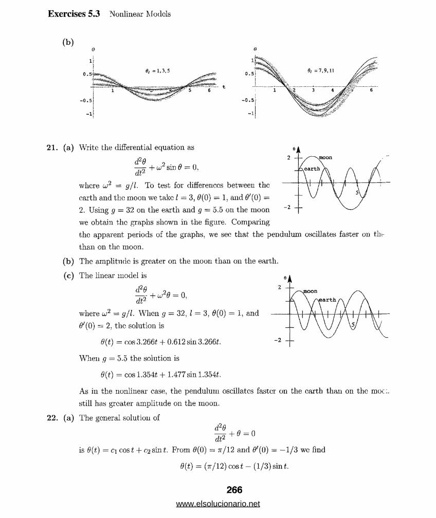
Exercises 5.3 Nonlinear Models
(b)e
if
21. (a) Write the differential equation as
ci2# 2 • a -^2 + w sm 0 — 0,
where u>2 = g/l. To test for differences between the
earth and the moon we take I = 3, 0(0) = L and (0) =
2. Using g — 32 on the earth and g = 5.5 on the moon
we obtain the graphs shown in the figure. Comparing
the apparent periods of the graphs, we see that the pendulum oscillates faster on the
than on the moon.
(b) The amplitude is greater on the moon than on the earth.
(c) The linear model is
where u>2 — g/l. When g — 32, I = 3, 0(0) = 1, and
0;(O) = 2. the solution is
0(t) = cos 3.266£ + 0.612 sin 3.2661
When g = 5.5 the solution is
6(t) = cos 1.3542 + 1.477 sin 1.3541
As in the nonlinear case, the pendulum oscillates faster on the earth than on the moc:.
still has greater amplitude on the moon.
22. (a) The general solution of
is 9(t) = ci cos t + c-2 sin 1 From 0(0) = 7r/12 and 0'(0) = —1/3 we find
0(£) = (7t/12) cost — (l/3 )s in l
266
www.elsolucionario.net

Exercises 5.3 Nonlinear Models
I b) We set 9(t) = 6(0) + O'[0)t + ^ " ( 0)*2 + ^d"1 (Q)ts H-- and use 9"(t) = — sin 6(1) together wiri.
0(0) = 7 r /1 2 and <?'(0) = — 1 /3 . Then
0 " (O ) = - s i n ( 7 r / 1 2 ) = -y/2 (>/3 - l)/4
and
f l " '( 0 ) = - cos 0(0) • 0'(O) = - c o s ( t t / 1 2 ) ( — 1 / 3 ) = V 2 ( V $ + 1 ) / 1 2 .
Setting $(t) = 0 we have tan* = tt/4 which implies = tan 1 (tt/4) ~ 0.66577.
Thus
m 12 3 8 72
(c) Setting tt/12 — i/3 = 0 we obtain tj - tt/4 « 0.785398.
id) Setting
12
1 V 2 (V 3 - l) ,
8fz = 0
and using the positive root wc obtain t\ tv 0.63088.
(e) Setting
n 1 V2(\/3— 1) .2 , V2 (\/3 + 1) 3
12 3 8 ' 'r 72
we find with the help of a CAS that t\ ~ 0.661973 is the first positive root.
(f) From the output we see that y(t) is an interpolating function on
the interval 0 < * < 5, whose graph is shown. The positive root
of y(t) = 0 near * = 1 is — 0.666404.
lg) To find the next two positive roots we change the interval used in
NDSolve and P lot from {t,0,5} to {t,0,10}. We see from the
graph that the second and third positive roots are near 4 and 7,
respectively. Replacing { t,l} in F indRoot with {t,4} and then
{t.T} we obtain *2 - 3.84411 and *3 = 7.0218.
From the table below we see that the pendulum first passes the vertical position between 1.7 .
1.8 seconds. To refine our estimate of 11 we estimate the solution of the differential equation
i.i. 1.8] using a step size of h = 0.01. From the resulting table wc see that t\ is between 1..76 a:..'
1.77 seconds. Repeating the process with h = 0.001 we conclude that t\ ~ 1.767. Then the period
the pendulum is approximately 4*i = 7.068. The error when using t\ = 2tt is 7.068 — 6.283 = 0.7>”
and the percentage relative error is (0.785/7.068)100 = 11.1.
267www.elsolucionario.net

Exercises 5.3 Nonlinear Models
h=0.1 h=0.01
tn en0.00 0.785400.10 0.78523
0.20 0.784070.30 0.780920.40 0.77482
0.50 0.76482
0.60 0.75004
0.70 0.729620.80 0.70275
0.90 0.66872
1.00 0.626871.10 0.576601.20 0.517441.30 0.448951.40 0.370851.50 0.282891.60 0.18497
1.70 0.077061.80 -0.040761.90 -0.168312.00 -0.30531
11 en
1.70 0.077061.71 0.06572
1.72 0.054281.73 0.042751.74 0.03111
1.75 0.019381.76 0.00755
1.77 -0.004381.78 -0.01641
1.79 -0.02854
1.80 -0.04076
h=0.0011.763 0.003981,764 0.002791.765 0.001601.766 0.00040
1.767 -0.000791.768 -0.001991.769 -0.00318
1.770 -0.00438
U . V; is is a Contributed Problem and the solution has been provided by the author of the problem.)
: a) The auxiliary equation is m2 4- g/t = 0, so the general solution of tlie differential equation
0(f) = ci cos t + oi sin ^ 1 1.
The initial condtiou 0(0) = 0 implies ci = 0 and $'(0) = wq implies 0 2 = . Thus.
&(t) = sin \/f
b) At 0njax, sin J g / i t — I, so
a ___ It _ m> Vb 
Chapter 5 in Review
Thus
m-w + vn, f— i 2h m.w + mb Vb= ■/«-. .
mb
(d) When ro/, = 5g, mw = 1kg. and h - Gem. wc have
1005
% n r 7nw - t m h r ~ r
vb = -T"V/2(980)(6) ~ 21,797 cm/s.
S ft, since k = 4
2tt/5. since \x" + 6.25x = 0
5/4 m, since x = — cos 4/: -f | sin 4£
True
False; since an external force may exist
False; since the equation of motion in this case is x(t) = e~^(ci + ctf) and x(t) = 0 can have at
most one real solution
overdamped
From ;r(0) = (\f2/2) sin 6 - —1/2 we see that sin<J> = —l/y/2, so is an angle in the third or
fourth quadrant. Since x'(t) = y/2cos(2t + <p)f x'(0) = \/2cos0 = 1 and cos 6 > 0. Thus <j> is in the
fourth quadrant and 6 = —tt/4.
y = 0 because A = 8 is not an eigenvalue
;j = cos 6x because A = (6)2 = 36 is an eigenvalue
The period of a spring/mass system is given by T — 2tt/u; where J 1 = k/m = kg/W, where k is the
spring constant, IF is the weight of the mass attached to the spring, and g is the acceleration due
U) gravity. Thus, the period of oscillation is T — (2-ivj\/kg)\/W. If the weight of the original mass
is W, then (2ir/y/Icg)VW - 3 and (2n/^/kg)VW ^S = 2. Dividing, we get V W /y /W ^8 = 3/2
)i' W = f (TT7 — 8). Solving for W we find that the weight of the original mass was 14.4 pounds.
(a) Solving + 6:r = 0 subject to x(0) - 1 and .^(O) = —4 we obtain
x = cos 41 — sin At = V2 sin (41 + Sn/4).
(b) The amplitude is \/2. period is tt/2, and frequency is 2/tt.
269www.elsolucionario.net

Chapter 5 in Review
(c) If x = 1 then t — rin/2 and t = — tt/S + mr/2 for n = 1, 2, 3, ... .
i. d) If x — 0 then t = tt/16 + mr/4 for n — 0, 1. 2, .... The motion is upward for n eve:,
downward for n odd.
i e) = 0
if) If x' = 0 then 41 3tt/4 = tt/2 + rar or t = 37r/lG + mr.
13. We assume that he spring is initially compressed by 4 inches and that the positive direction
.r-axis is in the direction of elongation of the spring. Then. from, ^x" + |a/ + 2x = 0, a?(0) = -•
e,r.d .r'(0) = 0 we obtain x = -|e“2/ + ±e"4*.
14. From x" + fix' + 64a? = 0 we see that oscillatory motion results if (32 — 25C < 0 or 0 < ,8 < 1l
15. From mx" -f 4a/ + 2x = 0 we see that nonoscillatory motion results if 16 — 8m > 0 or 0 < m
I*?. From ja;/; + x! + x = 0. .r(0) = 4. and 2/(0) = 2 we obtain x = 4e-2t + 10te~2t. If xf(t) = 0. '
■ = 1/10. so that the maximum displacement is x = 5e-0,2 ss 4.094.
1". ‘Anting |a/' + |a: = cos7* + sin7* in the form x" + Ta? = 8cos7it + 8sin7* we identify J 1 =
The system is in a state of pure resonance when 7 = 0/= ^64/3 = 8/\/3.
15. C’.early xp = A/uP suffices.
19. From ga/' + x' + 3x = e-t. x(0) = 2, and a?r(0) = 0 wc obtain xc = e~4i (ci cos2\/2i -f- C2sin2\ .
- = Ae~l . and1 I
21. ■■ a) Let k be the effective spring constant and .ri and X2 the elongation of springs ki and ■
: b) From ki = 2W and k2 = 417 we find 1/A: - 1/2VF-M/4W = 3/4VF. Then k = AW/3 = 4??;.
The differential equation mx" + kx ~ 0 then becomes x" -j- (4g/3)x = 0. The solution is
restoring forces satisfy k\xi = ^ 2 so a?2 = (k\/k‘2)xi. PVom k(x\ + ^2) = k\Xi we have
A-i + k2
1 1 1
k k 1 k2
270www.elsolucionario.net
Chapter 5 in Review
The initial conditions x(0) = 1 and x'(0) = 2/3 imply _ = 1
(c) To compute the maximum speed of the mass wc compute
x'{t) = 2y| sin 2^| t + ~ eos2y'| t and |.r'(i)| = y ■4 | + ^ | 3; - 1
From q" + 104g = 100 sin 501 g(0) = 0. and c/(0) = 0 we obtain qc = c-\ co* 1 —
jy = i sin 501 and
(a) q = — sin lOOt + 4$ sin 501
(b) i = — | cos 1002 + | cos 501 and
( c) q = 0 when sin 50t(l — cos50t) = 0 or t = nnjoQ for n = 0, 1, 2, ... .
i a) By Kirchhoff's second law.
L w +Rdl J r b q = m -
Using q'(t) = i(t) wc can write the differential equation in the form
L S + Ri + d g - B(th
Then differentiating we obtain
_ d2i di 1 .. ,
L d f i+ R dt + C , = E{t)-
lb) From Li'(t) + Ri(t) + (1 /C)q(t) = E(t) we find
Li' (0) + Ri( 0) + (1/C)q(0) = E{ 0)
or
Li'(0) + Ri0 + (l/C)q0 = E(0).
Solving for i'(0) we get
i'(0) = ~ [fi(O) - i go - Rio .
For A = a2 > 0 the general solution is y = ci cos ax + c-2 sin ox. Now
2/(0) — ci and y(27r) = ci cos 2itck + 0 2 sin 27ra.
< 0 the condition ,y(0) = y(2n) implies
C] = c\ cos 27ra + c% sin 2ttq-
which is true when a = \f\ = n or A = n2 for n = 1, 2, 3, ... . Since
y - — ac\ sin ax + ac% cos ax : —nc\ sin nx 4- nc2 cos nx,
271www.elsolucionario.net
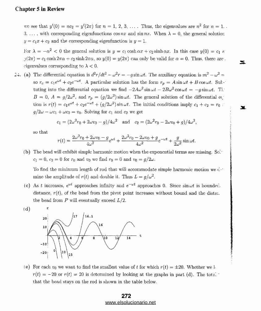
Chapter 5 in Review
wc see that ;i/(0) — nc-i = 2//(2tt) for n = 1, 2, 3. ... . Tims, the eigenvalues are n2 for n = 1. -
3. ... , with corresponding eigenfunctions cos nx and sinn;/;. When A — 0, the general solution
i) = cyx + C'2 and the corresponding eigenfunction is y = 1.
For A = —a2 < 0 the general solution is y = cj cosh ax + C2 sinh ax. In this case y(0) ~ ci a
7(2tt) = c\ cosh2-7ra -t- C2sinli27ra\ so y(0) - y(27r) can only be valid for a: = 0. Thus, there are .
eigenvalues corresponding to A < 0.
(a) The differential equation is d?r/dt2 - J 2r = —g siii^'i. The auxiliary equation is m2 — J 2 =
so rc -- c\ewt + A particular solution has the form rp = A sin -jjt + B cos u)t. Sub-'
tuting into the differential equation we find —2Aco2 sin cut — 2Bco2 cos cot = —gsiucot. TL'
Z? = 0, A — g/2'J2< and rp = (g/2ui2) smcot. The general solution of the differential ec
lion is r(t) = + C‘)€~xt + (g/2oj2) sm^t. The initial conditions imply ci + c-2 = ro
g/2u> — cuci +ujc2 = t’o ■ Solving for c,\ and C2 we get
ci = (2cj‘2rQ + 2-jjvq — g)/4co2 and c-2 = (2J2ro — 2lovq + g)/4u>2,
so that2uj2r0 + 2covq - g M 2u2r0 - 2wvq + g
C t" +9
sin cot.4!j02 ' 4i02 ' 2co2
(b) The bead will exhibit simple harmonic motion when the exponential terms are missing. So/
Ci = 0, c? = 0 for r\) and t’o wc find ro = 0 and vq = g/2d .
To find the minimum length of rod that will accommodate simple harmonic motion we t:-‘
mine the amplitude of r(t) and double it. Thus L = g/oJ2.
(c) As t increases. ew/ approaches infinity and e ~ ,jSt approaches 0. Sincc sin cot is bounded,
distance. r(t), of the bead from the pivot point increases without bound and the distai-
the bead from P will eventually exceed L/2.
(d)
fe) For each vq we want to find the smallest value of t for which r(t) = ±20. Whether we L.
r(t) — —20 or r(t) = 20 is determined by looking at the graphs in part (d). The tota.
that the bead stays on the rod is shown in the table below.
272www.elsolucionario.net

Chapter 5 in Review
Vo 0 10 15 16 .1 17
r -20 -20 -*20 20 20
t 1.55007 2.35494 3.43088 6.11627 4.22339
When t'o = 10 the bead never leaves the rod.
Valike the derivation given in (1) of Section 5.1 in the text, the weight, mg of the mass m does not-
appear in the net force since the spring is not stretched by the weight of the mass when it is in the
T-quilibrhun position (i.e. there is no mg — ks term in the net force). The only force acting on the
::iass when it is in motion is the restoring force of the spring. By Newton's second law,
(fx k■m —it = —kx or —T -I-- x = 0.
dt dt1 m
The force of kinetic friction opposing the motion of the mass in /.iN, where /i is the coefficient of
sliding friction and N is the normal component of the weight. Since friction is a force opposite to
:he direction of motion and since N is pointed directly downward (it. is simply the weight of the
mass). Newton’s second law gives, for motion to the right (V > 0) ,
2 , „
:-nd for motion to the left (V < 0).
d*xm —tit = —kx — imiq.
dt*
d?x
.traditionally, these two equations are written as one expression
d2x r / Am + ^ sgn(x ) + kx =
where //,. = ftmg and
, j 1. x/ > 0
Sgn(" ) = i- 1 , z' < 0.
273www.elsolucionario.net

6 Series Solutions of Linear EquationsSolutions About Ordinary Points
1. lim2u+lx"-l /(n + 1)
2nxn/nlim
2 n-|z| = 2\x\
n->oc n -\-
The series is absolutely convergent for 2|x| < 1 or |:cj < The radius of convergence is R
At x — — the series l)n/n converges by the alternating series test. At x = 3, the h
Y.^=i 1/n is the harmonic series which diverges. Thus, the given series converges 011 [—5,5).
100n+1(x + 7)n~l/(n + 1)!lim
100” (x + 7)n/u\ n -I-11
The radius of convergence is R = 0 0 . The series is absolutely convergent 011 (—00,00).
3. Bv the ratio test.
limk—>DC
(x - 5)fc+1/10fc+i 1 .= hm — \x
(x - 5)k/10k k—>3C 105| = ~ 5|.
The series is absolutely convergent for — 5| < 1. j;?: — 5| < 10. or on (—5,15). The rad:
convergence is R. = 10. At x = —5, the series (—l) fc(—10)&/10& = 1 diverges by tli-.-
term test. At x = 15, the series HfcLi(—l)A10fc/10fc = £feLi(—l) fc diverges by the nth term
Thus, the series converges on (—5.15).
00. x 7 14. lim.. I (k + l)!(x — l ) k+llim ---tt;----tt--.v—rsc-j k\(x — l)k
The radius of convergence is R = 0 and the series converges only for x = 1.
= lim (k + l)|.r - li =k—>00 I (}. x = 1
:r3 xQ x‘5. sm*cosa:= . r - - +12Q ^
;r4 ■v.61 - - - - -- -|-
2 24 720
x.2 X4~X COS X — 1 — X -S- ^ ----- ~ + T T —
I 2 6 24
x2 a:4 \ x'* x4
Y + 24- '" j = 1 - x + T ~ T
2x’Jj 2 x 4.r
= X 3~~ + ”l5"~~ 31T
+ . . .
1 1 5.r4 61a:6
COS X 2 4 6 1 x , ar x" ,1 - T + I T _ 6 T +
■ 1" Y + '4T + 6!
Since c o s ( tt/ 2 ) = cos(—tt/ 2 ) = 0, the series converges on (—tt/2, tt/2).
274
www.elsolucionario.net
Exercises 6.1 Solutions About Ordinary Points
. 1 — x 1 3 3 2 3>, ---------- — -----------T -I------ r — -----2 + x 2 4‘ 8 16''
Sinco the function is undefined at x = — 2, the series converges on (—2.2).
/. Let k — n — 2 so that n = k — 2 and
nc„x"+2 = '52(k- 2)ck_-2:rk.«=1 A—3
. I . Let k = n — 3 so that n = + 3 and
£ (2n - l)c„.x«-3 = £ (2k + 5)ck^ v k.n=3 fe=0
^ 2nc„xu 1 + ]T 6c„xTt+1 = 2 • 1 • c ^ 0 + 2ncnxn ~1 + j r 6cn;crt+1■i=l n-=0 n=2 «-=0
A.-— n— 1 k=n+\
OC oc= 2ci + £ 2(A< + l)cA-+iarfe + ^ 6cfc_irc/>'ft=i A— l
— 2ci + [2 (k + l)c/|._i + Gcfr-i]^ fc=i
£ ra(ra - l)cnxn + 2-J2 n(n - l)c„xn-2 + 3 ]T nc-Tl.?;n■;=2 n=2 «=1
OC- oo ocncnxn
r i= 2 r/,=4 n=2= 2-2-lc.2.r° + 2 • 3 - 2c3;ia + 3 • 1 • Clx' + £ n(n - l)c„xn +2 ]T n(n - l)c„,xn-2 +3 £
fc ~-n. fe=n—2 At—??-
oc oc oc= 4c2 + (3ci + 12cs):r + ^ fc(fc - l)cA.:r/,: + 2 + 2)(k + l)cfc+2xfc + 3 fccfc.xfc
k=2 k=2 h=2oc
k— 4c*2 -+- (3ci + "1 2c;3)x + [(fc(fc — 1) + ik)C}- + 2(A- -r 2)(fc + l)Cju_2]hi=2
= 4c2 + (3ci + 12^3)x + [A?(A; + 2)q. 4- 2(fc + 1)(A; + 2)cJiu_|_2j ^k=2
oc
£ (- l)n+1:rn“\ / = 2 (-1)?<+1 (« - l)a?Kri~ 1 n=2
275www.elsolucionario.net
Exercises 6.1 Solutions About Ordinary Points
(* + 1 ) / + y’ = (x + 1) £ ) (- l)"+1(n - 1)*"“2 + E (-1)”+V *“ ‘n=2 n=1
OC oc oc
= E t - 1)" " 1 - - + E ( - 1)"+1(n- - l )x1l~2 + £ ( - i ) n+,®n_1n=2 ■n=2 n = 1
oc DC OC= —;c° + ,t° + (- l)n+1(n - l)xn_1 + £ (—l)n+1(n - I)®”" 2 + £ (- l)n+1.
U = 2 7 7 . - 3 ? ? , = 2
fc=n—1 k=n— 2
oc DC
h=n—1
- £ ( - l ) * +2fcc* + E ( - l ) fe+3(fc + l)a’fr + 53 (- l)*+2a?A
oc
k=1 A-=l
= £ [(-l)&+2fc - (-1 )k+2k - (- l )k+2 + (- l)A'+2j xk =k=1
1 , / _ y -' (—1)”'2ti 2??.—l // _ y - (—l ) ” 2n (2n — 1) o»-2
_ i= i 22,1()i!)2 * * - ........... .
xy" + y' + xy = £(__l )K2n (2n 1) v 2 n - i j_ v ' ( l ) ft2n ^ 2n -i y - ( l ) n ^Sn+i
xy . 2«-l , y-
22”(n!)2 +ir o 22nN )2
k .= n k=n A:=n—'l
= Efc=l
oc
= Efc=l
(—l) fc2fc(2fc - 1) (—l) fc2A’ (- 1)fc—l
22A(A*!)2
(—1)*‘(2A;)2
22*(fc!)2 1 22*-2[(Jfe - l)!]2
(- 1)*
;r, 2 f c -
= £ ( - Dfc=1
22*(fc!)2 22fc-2[(fc-i)!]5
(2A;)2 - 22A;2
^ - 1
o2A.-a.n2 .r2fc“ ' = 0
15. The singular points of (x2 — 2b)y" + 2xy' + y = 0 are —5 and 5. The distance from 0 to e::..
these points is 5. The distance from 1 to the closest of these points is 4.
16. The singular points of (x2 — 2x + 10)yw + xy' — Ay = 0 are 1 4- Zi and 1 — 3i. The distance
to either of these points is \/IO. The distance from 1 to cither of these points is 3.
IT. Substituting y = Y^Lq cnXn into the differential equation we have
y" ~ xy - £ n(n - l)cna;,t 2 - £ cnx'l+l = £ [k + 2)(A: + l)ck+2xk - £ ck- \ x :71=2 n=0 A’=0 k=l
k = n —2
oo
k=n+1
= 202 + E [(* + 2)(A. + l)c*+2 - Ck-i]xk = 0. fe=i
276www.elsolucionario.net
Thus
O2 = 0
( k + 2 )( fc + l)C fc j-2 — (:k—1 = 0
Exercises 6.1 Solutions About Ordinary Points
and
Choosing cq = 1 and ci = 0 we find
C3 = 6
C4. = = 0
06 = ISo
and so on. For co = 0 and ci = 1 we obtain
C3 = 0
1
C i ~ 12
Cs = Cq = 0
°7= 504
and so on. Thus, two solutions are
W = 1 + r 3 + IiOlli + '" “ d W = 1' + ^ + 554i7 + " "Substituting y = (‘nxn into the differential equation we have
OO OO oc OO
y" + x2y = n(n - l)cnxn~2 + c , , ^ 2 = J ] (A- + 2)(* + 1)^+2-/ + c*-2**n=2 n= 0 fc=0 A-=2
A:=n— 2 fc=n+2
oc
= 2c-2 + 6C3X + ^ [(k + 2)(k + l)cft+2 + c/j_ 2]xfc = 0. k=2
Thus
C2 = C3 = 0
(A: + 2)(& + l)c:fc+2 + ck~ 2 = 0
and
C 2 = _ (A; + 2)(A: + l ) Cfc~ 2! ^ = 2 ’3 ’4 ’- ■ • •
277www.elsolucionario.net
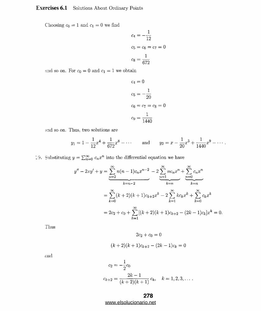
Exercises 6.1 Solutions About- Ordinary Points
C'lioosing c:q — 1 and c\ = 0 we find
C ,= _ l2
C5 = Cq = C 7 = 0
C8 = 672
and so oil. For co = 0 and c.\ = \ we obtain
c.\ — 0
1
C5 = “ 20
CQ = C7 = eg = 0
1
1440
and so on. Thus, two solutions are
* = a , ld 3/2= * - s * 5 + l a o *9 - ■ ■ ■
9. Substituting y = Y,n=l) cn%n into the: differential equation we have
y" - 2xy' + y = J 2 n(n - l)c„xn_2 - 2 £ ncnxn + £ ctkxnn= 2 i i — 1 0
... J v “ ^k = n —2 h = n k—n
OC oo oc= + 2)( ': + l)ck+2xk ~ 2 k.CkXk + ^ C iT
A.=0 A:=l fe=0
= 2c.‘2 + l ) efc-i-2 — (2A- — l)cfc]:r* = 0.A-=l
Thus
111(1
2c2 + Co = 0
(* + 2)(fc + l)cA:+2 - (2A;-l)c* = 0
1C2
2k — 1
C,0+2 = (fc + 2)(fc + l) Ck> k = 1? 2’3>''
278www.elsolucionario.net
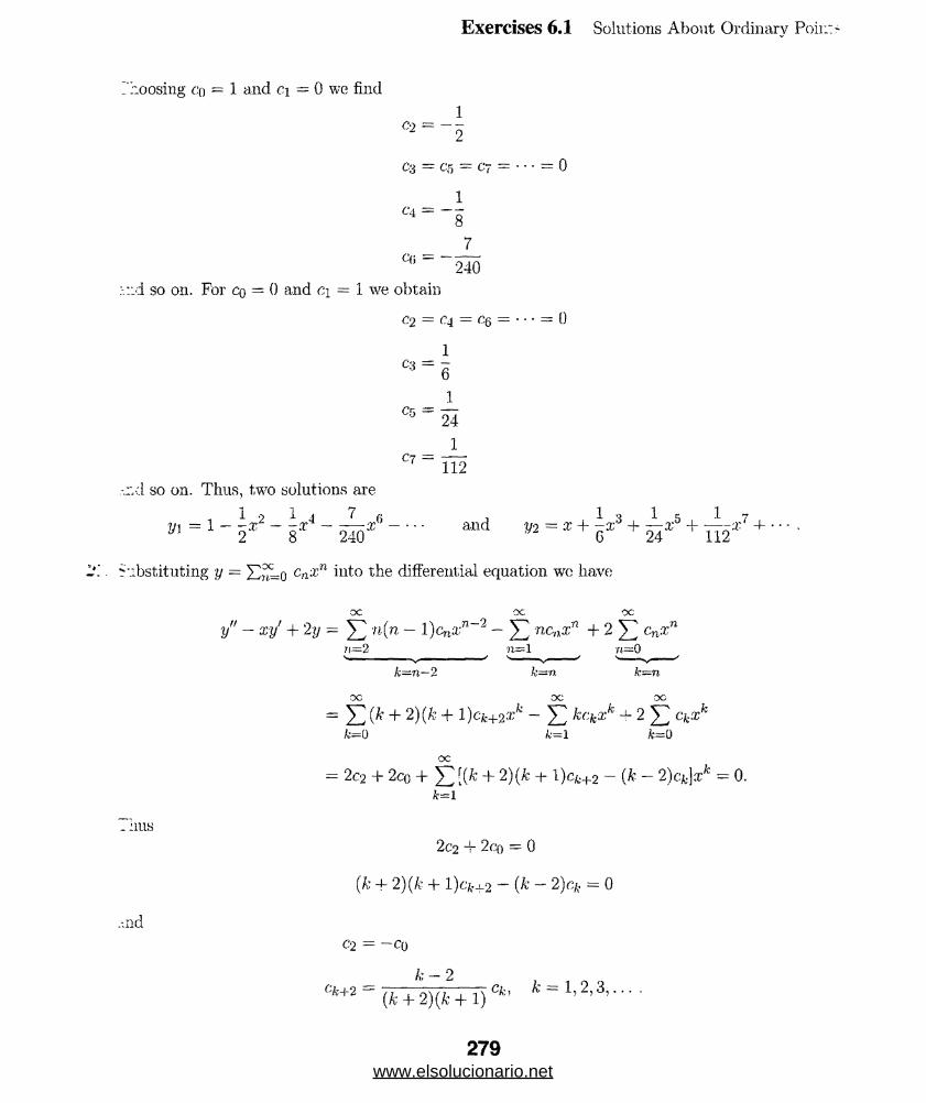
Exercises 6.1 Solutions About Ordinary Poii:>
~";:oosing co = 1 and ci = 0 we find
c'4 = "8
1
7co =
240
:-::d so on. For cq = 0 and c\ = 1 we obtain
C2 = c 4 = ce = • • ■ = 0
1
1
I
1
C 7 = m
C3 6
C5 24
-;vd so on. Thus, two solutions are
w = 1 _ - X - - g* - — x - • • • and y2 = X + -X + -X- + — *•
. Substituting y -; I^Lo cnZn iuto the differential equation wc have
u" - xy' + 2y - Y , n(n - l)cnXn~2 - ncnxn + 2 cnxnn=2 n=l n—0^ >• V >•
. :ius
.-.nd
k —n —2 k = n fc=n
(A* + 2) (A- + l)cjfc+2s* - J2 kck'xk + 2 S c‘fe;rfcA;=0 A;=l Jfe=0
OC
2c2 + 2cq + 5Z [( 2) (A; ■*" ^)cA;+2 — (A’ — 2)c ]:cfc = 0. fc=l
2c2 + 2co = 0
(A- + 2) (A- + l)c>+2 ~ (A' — 2 )(■:/,, = 0
C2 = -C o
Ck+2 = {k + 2)(k + l) Cfc’ k = 2; 3? • • • •
279www.elsolucionario.net
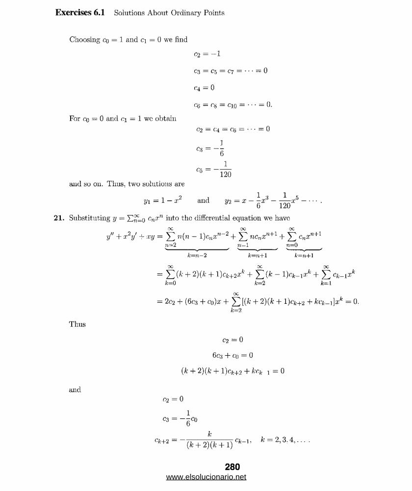
Exercises 6.1 Solutions About Ordinary Points
Choosing cq = 1 and c\ = 0 we find
For cq = 0 and c\ — 1 wc obtain
C'2 = --1
C3 = C'5 = C7 = • • • = 0
('4 — 0
<"'6 ” 8 = CJ.0 = ’ ' ’ = 0.
C‘2 ~ C4 = Cq = • ■ • = 0
cr, = 120and so on. Thus, two solutions are
2 1 * 1 - yi = l - x and y2 = x - ~x' - — ar°--- .
21. Substituting y — cnxn into the differential equation we have
y" + x2y’ -f- xy = ]T n (n ~ nCnXn+1 + £ c„,rri+1n—2 n — 1 n =0
Thus
k —/ —2 A.’—71 ~I— 1 k‘—f 1
= + 2)(k + l )ck+2Zk + Y .(k ~ 1)(‘k-rxk + J2 Cfe_i:xk k=0 k=2 A;—1
— 2c-2 + (6c‘3 + c‘o)it’ + ^ 2 [(A’ + 2)(k + 1)(-a-+2 + A:c _i]a,fc = 0 .k=2
C-2 — 0
6c;j + C() = 0
(k + 2)(k + l)c/~+2 + k-c'k l = 0
and
C-2 = 0
C3 = ~ rc06
280www.elsolucionario.net

1
C* = -6
C.'l - C5 = 0 1
- -7Z4o
and so on. For co = 0 and ci = 1 we obtain
c3 = 0
1
C1 = " 6
Exercises 6.1 Solutions About Ordinary Points
Choosing co = 1 and c\ = 0 wc find
cr, = cq = 0
CJ 252
•aid so on. Thus, two solutions are
i ^ H , 1 6 i ^ 4 • ^ 7
+ 45* - - and w = ^ 252*
Substituting y = c"x" ^lto differential equation we have
OC OO OC
y" -I- 2:ry' + 2y = £ n (n — l)cnxn~2 + 2 £ ncnxn + 2 £ °nXnn=2 n=l n=0
A:=n—2 k=n k—?7.
"Xi oc oc
= £ 'r 2)(A’ + l)cfc+2^ + 2 £ kc.kXk + 2 £ CfcE*A;=0 fc=l fc=0
= 2c2 + 2co -r £ C( 2)(A: + l)c^_2 + 2(A- + l)cfc]:u = 0. fc=l
Thus2c2 + 2co = 0
(.k + 2 )(k + l)cfc+2 + 2(k + l)c* = 0
C-2 = —Oo
c/,--r2 — 9 Cfc, A: = 1.2,3,... .
281
:id
www.elsolucionario.net

Exercises 6.1 Solutions About Ordinary Points
Choosing co = 1 and c\ = 0 we find
02 = -1
— Cf, = C-7 — • • • = 0
1
C1 = 21
6
and so on. For Cq = 0 and c\ = 1 we obtain
c2 = c4 = ce = • ■ ■ = 0
C3 = - 3
c'5 15
C7
24-
4
8
105
and so on. Thus, two solutions arc
1 4 1 6 i 2 o 4 x 8 <ryi = 1 - ar + -x4 - -x6 + •• • and y2 = x - -xA + — xa - — x‘ + - • • .
2 6 3 15 105
23. Substituting y = Z)nLo cnxn into the differential equation we have
OC OC OG
(x - 1 )y" + y' = Y I n (n - l)<vrr'_1 - £ n{n - 1 )cnxn~2 + ^ nc-nX71-1n—2 n—2 7i=l
r?, — 1 k = n —2 A:= 77- — 1
= 5 3 (fe + l)Acjfe+ia:* - j^ (k + 2)(k + + X ) ( fc +
Thus
and
— —2c‘2 + ci + 52 [{k + 1) A- 1 — (k + 2)(fo + l)c*;+2 + {k + 1)c/h-i fc=i
—2c-2 + ci = 0
(k + l)2Cfc+i — (k + 2) (A: + l)qu+2 = 0
1C2 = -Cl
k + 1 , 1 0 0 °k = /■> _(_ 9 c*^l> k ~ lj 3... . •
282www.elsolucionario.net
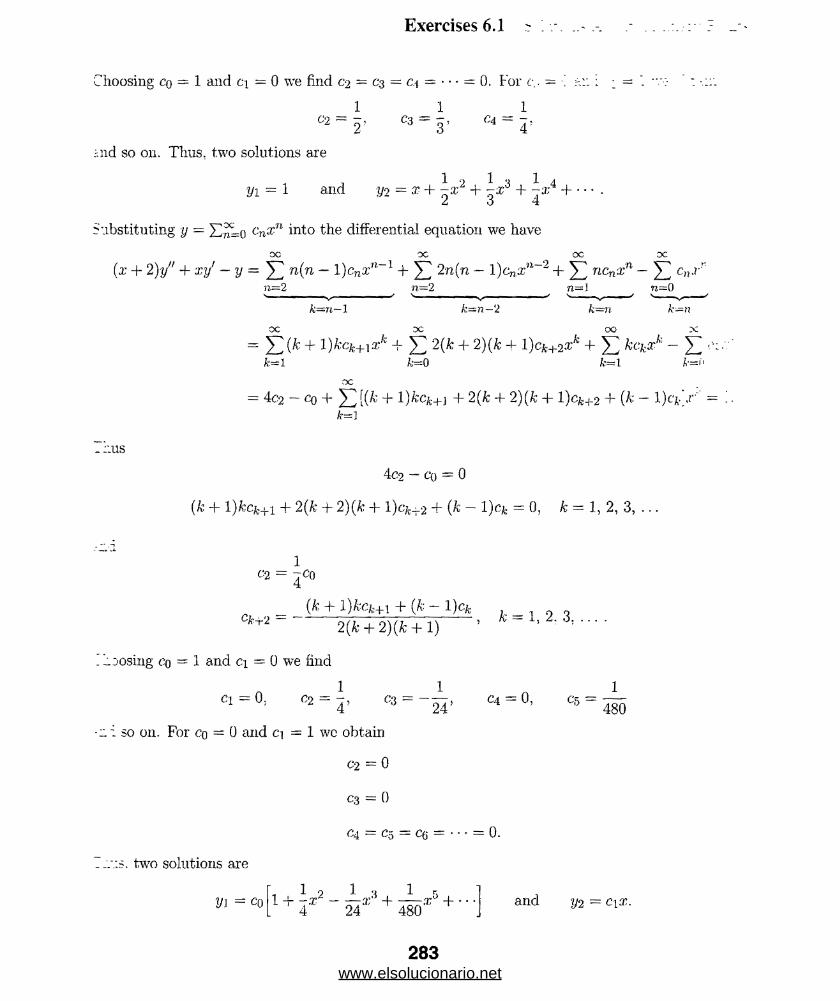
Exercises 6.1
Choosing co = 1 and a = 0 we find C2 = C3 = c.\ — • • • = 0. For c,. = •! : : =
1 1> =
-nd so on. Thus, two solutions are
C2 = C3 = C4 =2 3 4'
yi = 1 and yo = x + -x2 + + ^a;4 H-- .2 o 4
Substituting y = X ^ o cn^n into the differential equation we have
DC OC OC- OC
(x + 2)t// + xy' - y = J 2 n(n - l)cnxn_1 + ]T 2n(n - l)c„2;n_2 -f 53 ncn®n - X] c"r "n= 2 •n= 2 n=.l n=0>------ v------ ' '------- -------' v-------/ v-- v-- /
k = n — 1 k = n —2 k = n k —n
O C O C OO X
“ 5 3 + l)Acfc+ia:fc + 53 2(A; + 2)(A: + l)c*;+2®fc + 53 — XI 'fc=i fc=0 fc=l A-=m
= 4^2 — co + 53 + l)A"Cfc+j + 2{k 4- 2){k + l)cfc+2 + (k — 1 ) c.‘a- .t" ;
k-i
. :;us
4c2 — co = 0
(k -f l)fccfe+i + 2(k + 2)(k + l)cfe-i-2 + (A — l)cfc =0 , k = 1, 2, 3, ...
102 = 4C0
(ft + l)fec&+1 + (fc - l)cfc 0
°*+ 2 ---- 2(* + 2)(* + l)--- ' -.........
nosing co = 1 and ci = 0 we find
c i= 0, C2 = -, C3 = — 24-’ C4 = 0’ C5 = 480
. i so on. For co = 0 and c\ = 1 wc obtain
C2 = 0
cs = 0
C4 = C5 = cG = • • • = 0.
:.7.s. two solutions are
1 « 1 1 . iand 1/2 = c\x.V\ = co
1 1 9 I 'i 1 r>1 + 4r - 5 ^ + m x +
283www.elsolucionario.net

Exercises 6.1 Solutions About. Ordinary Points
25. Substituting y = cn' n into the differential equation we have
OC OC1 o c o cy" - (x + 1 )y' - y = ]T n(n - 1 )cnxa~2 - ]T ncnxn - ncnxn_1 - £ CnXn
71=2- n=l n= 1 /?•—0 V ^ V s ------ ' >--- -'
Thus
and
k = n —2 k —n k ~ r i— 1 k = n
Y , ik + 2) (k + l)ck+2xk ~ J2 ***** ~ J 2 (k + 1 )cfc+i xk - E ckx>'k - 0 A—l k= 0 k=D
2C2 — c i — co + £ [(A; 4- 2 ) ( k + l)c / ._ 2 — ( k + l ) c ^ + i — (A: +k=l
2C2 — Cl — Co = 0
(A’ + 2)(A: -j- l)c*+2 — (k + l)(c*;+i + c&) = 0
Cl f coC-2 = 2
_ C&+1 ”1” j 1 O o“ +2 - k + 2 ■- k = L2 ’ i .......
Choosing cq = 1 and ci = 0 we find
1 1 1
°2 ~~ 2’ - q-.01 = 6
1 we obtain
1 l 1
C’2 ” 2'C3 = 2 ,
°4 ~ 4
and so on. Thus, two solutions arc
1 9 1 -j 1 a 1 2 1 , 1 4y1 = l + -x‘J 4- -ar + -af H---- and y2 = x + -x2 + -x* -x4 +
26. Substituting y = 2 ?Lo cnx11 into the differential equation we have
•oo -oc oc-(V2 + l) y" - 6y = J2 n(n - l)cnxn + £ n(n - l)cnxn~'2 - 6 £ cuxn71=2 71=2 71=0
k=n k=n—2 k=n
= Y . H k - t)ck.xk + £ (* + 2)(k + - 6 5Z ckxh k=2 k~ 0 k= 0
oc
= 2c2 - 6c*o + ( 6c*3 - 6c i)rc + £ [(V2 - k - 6) ck + ( k + 2 ) ( k + l j c ^ l .*k.= 2
www.elsolucionario.net
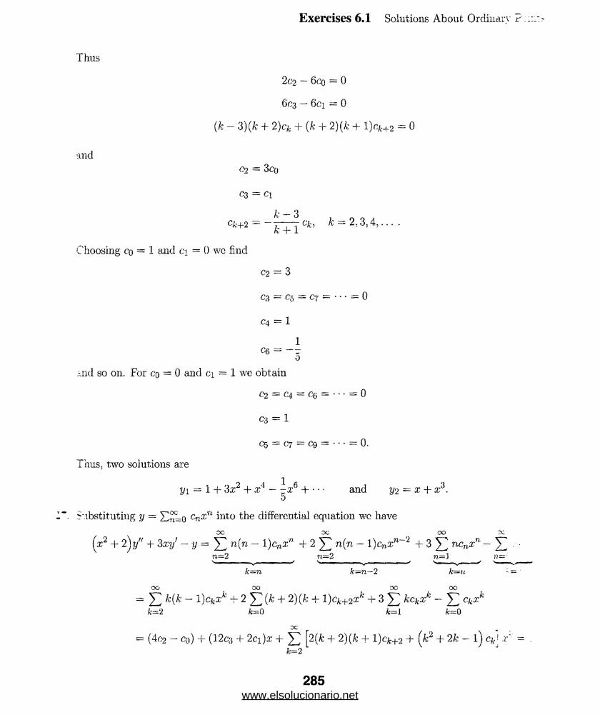
Exercises 6.1 Solutions About Ordinary r
Thus
2 c 2 . — 6 c o = 0
6c3 — 6ci = 0
(k — 3)(k + 2)c& + (k + 2) (ft 4- l)c -+2 = 0
and
02 = 3co
C3 = Cl
ck+2 = - ■Try fc = 2 .3,4,... .Choosing co = 1 and ci = 0 we find
C2 = 3
C3 = Co = C7 = • • ■ = 0
C4 = 1
1C6 — T
o
And so on. For cq — 0 and c\ = 1 we obtain
C2 = C-4 = C6 = • • • = 0
C3 = 1
C5 = 67 = 09 = • • ■ = 0.
Thus, two solutions are
1Vi — 1 + 3x2 + rc4 — -x6 H-- and y2 = x + x*.
5
I". Substituting y = X^Lo cn.rn into the differential equation we have
(x2 + 2)y" + Sxyf — y = 52 n(n — 1 )cnxn + 2 52 n (n ~ l)cnXn~2 + 3 52 ncn^n — 52n=2 n=2 n-=] n=:‘
/c=??, k = n —2 At=/a
00 00 OC- 00
= 52 - i)cfc£c* + 2 53 (& + 2)(* + + 3 13 kckzh - 53 ckxkk=2 &=0 fc=l A;=0
OC
fc=2— (4c2 — cq) + (12c*j 4- 2ci)x 4- + 2)(& + l)c/-_j_2 — 1 * x ' —‘ 2
285www.elsolucionario.net
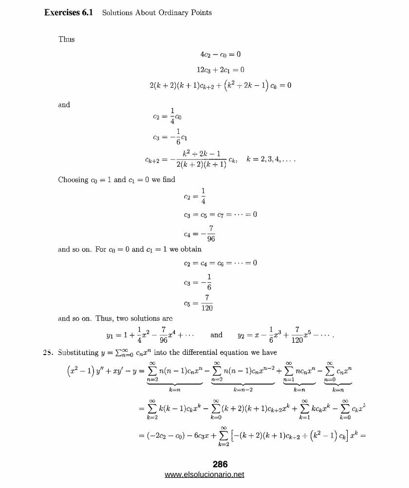
Exercises 6.1 Solutions About Ordinary Points
Thus
4c2 — co = 0
12c3 + 2c\ = 0
2{k + 2)(k + l)ck+2 + (jfe2 -i- 2k - l) ck = 0
and1
0 2 = j C Q
1Cs = -~c 1
6
i„2 0 7._ 1
Cfc+2 = ~2(fc + 2)(fc + 1) fc = 2-M .......
Choosing co = 1 and ci = 0 we find
1
fl2 = I
C3 = C5 = C7 = • • • = 0
_ _ 7 _
04 ~ _ 96
and so on. For co = 0 and c\ = 1 we obtain
C2 — C4 = C(j = • • • = 0
103 = - g
°5 = 120
and so on. Thus, two solutions arc
, 1 9 7 4 , 1 , 7 5
»' = 1 + i x' ~ w x + ' " and V2 = x ~ r ' + m x' -■■■■
2S. Substituting y = cn%n into the differential equation we have
oc oc 00 oc(ar2 - l) y" + xy' - y = 53 n(n - 1 )cnxn - 53 n(n - l)cnxn~2 + £ ncnxn - £ cnxn
77-=2 n= 2 n = \ n = 0
k—n k —n —2 k —n k—n
oo oc oo oo
= 5 3 _ - 5 3 (fc + 2) (a + 1)ck+2xk + 5 3 kckxk - 5 3 Cfca-*'fc=2 k=0 &=1 fc=0
k= ( - 2C2 - co) - 6c3x + 53 [“ (* + 2)(k + l )ck+2 + (k2 - l) ck
2
286
2; =
www.elsolucionario.net

Exercises 6.1 Solutions About Ordinary Points
Thus
and
—2c2 — Co = 0
—6C3 - 0
— (k -+- 2)(k + l)Cfe+2 + (k — l)(k + = 0
C2 = — 2C()
C3 = 0
k ~ 1 ,C*+2 = ^ 9 Ck'‘ k = 2’ 3? 4;
Choosing co = 1 and ci = 0 we find
1C2 - —2
C3 = (‘5 ~ c7 — ‘ ‘ • = 0
1
Q = “ 8
and so on. For cq — 0 and ci = 1 we obtain
c-2 = c,i = ce = • ■ • — 0
C3 = C5 = C7 = • • • = 0.
Thus, two solutions are
1 12/1 = 1 — -x2 - -x4--- and jfe = s.
Substituting y = Y.^=q cr,xn into tlie differential equation we have
•oc oc oc oc
(x - 1 )y" -xy' + y = Y n (n ~ 1 )cn®"_1 - Y n(n ~ )(-'nXn~2 - Y ncnxn + Y cnx,n
__n=2 n=2 n=1 n—0
fc=7i—1 k-n—2 k~7i k~nOC OO OO o o
= Y _ 53 + 2)(^ + 1)ck+2Xk - Y kck%k + Y ckxkk—i k=0 k= 1 k~0
o c— —2c2 + co + Y (k + 2)(k + 1)^+2 + (k + l)kck+i — (k — 1 )ch\xk = 0.
fc=l
Thus
—2c2 + co = 0
287www.elsolucionario.net
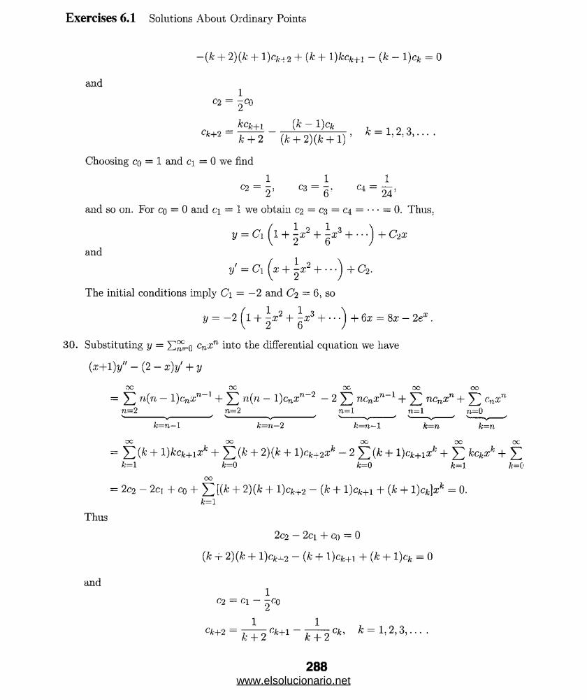
—(k + 2)(k + l)cfc-i.2 -f- {k + l)/ccfe+i — (k — l)cfc = 0
Exercises 6.1 Solutions About Ordinary Points
and
C 2 = 2Co
_ kck+1 _ (k - l)ck
k+2 k + 2 (jfc + 2)(fc + l) ’
Choosing cq — 1 and C] = 0 we find
1 1C2 = j , C3 = z , C4 =
and so on. For cq = 0 and ci = 1 we obtain c2 = C3 = C4 = • • • = 0. Thus;
y = Ci ^1 + ] x2 + jU '3 H-- j + C2x
and
1/ = Ci 'x + -x2 + • • + C2.
The initial conditions imply C-\ — —2 and C2 — 6, so
y = — 2 ^ x2 + ^.r3 + • • + 6x = 8x — 2ex .
30. Substituting y = cnxn into the differential equation we have
(x+l)yH - (2 - x)y' + y
O C O C O C OO OO
- Y n (n - l)cn^n-1 + Y n(n - l)cnxn~2 - 2 Y ncnxn~l + Y ncnxn + Yn=2 n=2 n= 1 n= 1 ri=0s------ v------ ' '------ V------ ' v--- -
k=n~l k—n—2 k=n—1 k—n k=n
O C OC OO o c oc
= Y + l)h ck+ixk + Y i f t + — 2 £ (fc -f l)cjk+ixfc + Y kckXk + Yk= 1 fc=0 A;=0 fc=l k= 0
oc-
= 2c2 — 2cj + co + £ [(A; + 2)(A: + l)cfc_j-2 — (^ + l)c^+i + (k + 1 )c^xk = 0. fc=i
Thus
2c2 — 2ci + Co = 0
(k -j- 2) (A; + l)cfcj-2 — (k + 1 )cfc_|_i + (A; + l)c£ = 0
and1
C-2 = Cl ~ jCq
c*+2 = ^ T 2 ':*+1“ fcT2c'!• * = 1 -2' 3.......
288www.elsolucionario.net
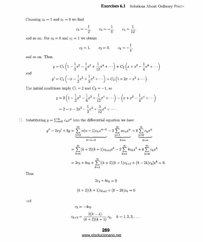
Exercises 6.1 Solutions About Ordinary Poir.t-
Choosing co = 1 and c\ — 0 wc find
02 = - 2 ’ C3 = " 6 : C'1 = 12'
and so on. For cq = 0 and c\ — 1 we obtain
oi = 1, C3 = 0. C4 = —4
and so on. Thus,
y = C\ (1 - ~.x2 - + ~.'c4 H-- j + C-2 (a + x2 - ^x4 + ■
and
l/ = C i(- z- | .T 2 + ^c3 + ---) i-C2 (l + 2x-x3 + •••).
The initial conditions imply C\ =2 and C2 = — 1, so
y = 2 {l ~\x2-\x* Jr ^ ;r4 + ‘ " ) ~ (x + x 2 -\x4+---
= 2 - x - 2 x 2 - + ^-a:4 H-- .O 1Z
Substituting y = X ^ o cnXn into the differential equation we have
00 00 oc
y " - 2x y ' + 8y = 5 3 n (n ~ l ) cn.£n_2 - 2 5 3 n c ux n + 8 5 3 c /i .'Cnj?.=2 /t—1 n=0
Thus
And
k —n —2 A’—rt fc=rc
53 (fc + 2) (fc + l)cjfc+2.x& - 2 53 *Cfcit:fc + 8 53 Cfc®*fc=0 Ar—1 /c=0
OC2c2 + 8co + 51 [(k + 2)(* + l)ck+ 2 + (8 - 2k)ck]xk = 0.
fc=i
2C2 "I- 8co — 0
(fc + 2)(fc + l)Cjfc+2 + (8-2fc)C* = 0
C-2 = —4Co
2(fe - 4) t = 1 9 o'*+2 (A: + 2)(k + 1) 'fc: 1>2>3--
289www.elsolucionario.net

Exercises 6.1 Solutions About Ordinary Points
Choosing cq = 1 and c\ = 0 we find
C2 = “ 4
c3 = C5 = C7 = • • • = 0
43
C6 = C8 = CiQ = • • • = 0.
C4 = —3
For cq = 0 and c\ = 1 we obtainC2 = C4 = c6 = • • • = 0
C3 = -1
1
05 ~ 10and so on. Thus.
andy — Ci ^1 - 4 x 2 + ^ x 4 j + C-2 ( x - x 3 + ^ x 5 H-------^
y' = Ci 8x + y x 3) + C2 ( l - 3x2 + ^x4 + ■••).
The initial conditions imply C\ = 3 and C2 = 0 , soy = 3 ( l - 4x2 + f*<) = 3 - 12x2 + Ax4.
32. Substituting y = CnXn into the differential equation we haveOC OC OC'
(x2 + 1 )y" + 2xy' = 52 n(n ~ l)cn^n + 52 n(n ~ l)cV ' n_2 + 52 2ncnx7n=2 n=2 n= 1 .. ■■■ —..... N ------ ' s--- ----
Thus
k—n k=n—'2 k—nOC 'OC o c
= 52 k(k - 1 )ckxk + 5 2 (A: + 2)(k + 1 )c ^ 2xfe + 52 2kckxkk= 2 fc=0 A;=l
00= 2c2 + (6C3 + 2ci)x + 5 2 + 1)CA: -r ( + 2)(fc + l)cfc+2]x = 0 .
fc=2
2c2 = 0
603 2c.t = 0
k(k + 1 )ck + {k, + 2)(k + l)ck+2 = 0
290www.elsolucionario.net
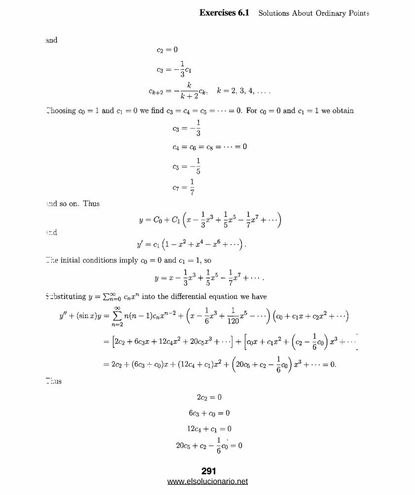
Exercises 6.1 Solutions About Ordinary Points;
and
c2 = 0
C3 = - 3C1
Ck+2 —k
Ic + 2ck: k = 2, 3, 4, ... .
□loosing Co = 1 and ci = 0 we find C3 = C4 = eg = • • • = 0. For co = 0 and c\ — 1 we obtain
103 - -3
C4 = cq = eg = • • • = 0
1C5 =
5
C71
-.rid so on. Thus
y = Co + C\ (ar - | x 3 + gar5 - ± x 7 +
y' = ci ( l — x2 + ar4 — x6 H-- ) .
The initial conditions imply Co = 0 and ci = 1, so
1 o 1 er 1 7y = * - r + s 1 ' ■ r + ' " -
Substituting y — Y,^=q cnxn into the differential equation we have
QO / I ”1y" + (sin x)y = £ n(n - l)c„.xn_2 + (re - -x3 + — a;5 - • co + C \X + C2X '
+ cox + Ciar + ( c2 - -cq ) X' -t-= 2c2 + 6C3X + 12c4X 2 + 2OC5X3 H-------
= 2c2 + (6c3 -f- Cq)x + (12C4 + Ci)x2 + ( 2OC5 + C2 - ^Co^ x3 H---= 0.
_ r.us
2c2 — 0
603 + co = 0
12c4 + ci = 0
20c5 + C2 - ^ c o = 06
291www.elsolucionario.net

Exercises 6.1 Solutions About Ordinary Points
and C2 = 0
1C3 - -gC0
1C4
= “ I2 C1
1 1C5
= “ 20C2 + 120C°‘
Choosing cq = 1 and c\ = 0 we find
1C‘2 — 0. C*3 = — —. C'4 = 0. C-} =
6 120and so on. For cq = 0 and ci = 1 we obtain
C2 =0, e3 = 0, c4 = - — , c5 = 0
and so on. Thus, two solutions are
1 o 5V\ = 1-- z -I--- x° +y 6 120
1 4and y2 = x- — x* +
34. Substituting y — 2i£Lo °n^n into the differential equation we have
OC
» n -2y" + exy! - y = £ n(n - l)cnxrn = 2
i i
n=0+ ^1 4- x + —x2 + —a;0 + • • • j ^ci + 2e2&‘ 4- 3c3£2 + 4c*4X + • • •'j —
]2” ' 6
2c2 + 6c3.r + 12c4.-r2 + 20cr);r'{ + •
+1
C\ + (2c2 + Ci)x -f ( 3C3 + 2c2 + ~ci) x2 H-- - [cq -f Cl X + (>2X2 +
= ( 2c2 + c i — cq) + (6c3 + 2c2)x + ^ 12c4 + 3c3 + C2 + = 0.
Thus
2c2 + Cl — Cq = 0
6c3 + 2c2 = 0
12C4 + 3C3 + C2 + ~C\ = 0
292www.elsolucionario.net
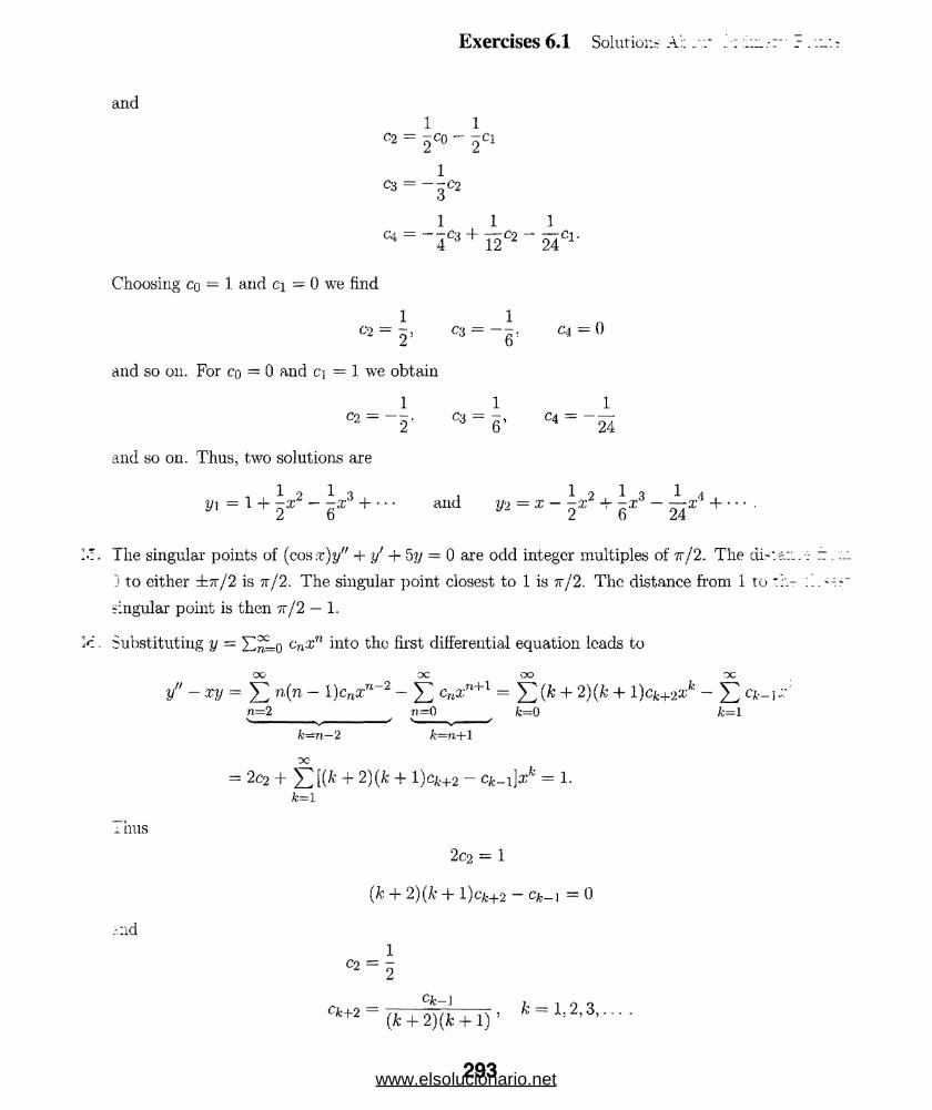
Exercises 6.1 Solutions A::
and
C 2 =
2C0" 2Cl
1C 3 =
“ 3C2
1 1 1C 4 = - 5 C 3 +
12C2“*24C1
Choosing cq = 1 and c\ = 0 we find
1 1 n2 6
and so on. For co = 0 and cj = 1 we obtain
1 1 1 C2 = - 2 ' C3 = 6 ’ C“ ” _ 24
and so on. Thus, two solutions are1 9 1 3 I 0 I 3 I 4
yi = 1 + 2® -g® +*•• and m = x ~2 ^ 2A
The singular points of (cos x)y" + 1/ + 5y = 0 are odd integer multiples of tt/2. The di> J to either ±7t/2 is tt/2. The singular point closest to 1 is tt/2. The distance from 1 to
singular point is then tt/2 — 1 .Substituting y = On%n hito the first differential equation leads to
OC- OC OO o cy" - xy = Y n ( n - 1 )cnxn~'2 - ] T cn * n + l = Y ( k + 2 ) ( k + l ) ck+'2Z k ~ Y
n—2______ ^ ^ n-0 k=0 k=l
k—n—2 /c=n+l
oc-= 2c2 + Y P + 2)(fc + l ) c k+2 - ck-i]xfc = 1.
k=1
j. mis
r.lid
2C2 = 1
(A: + 2)(ft + l)cjfc+2-cA-_] =0
1
C 2= 2
Cfc+2= (* + 2)(fc + l ) ’ fc = 1*2.3----
293www.elsolucionario.net
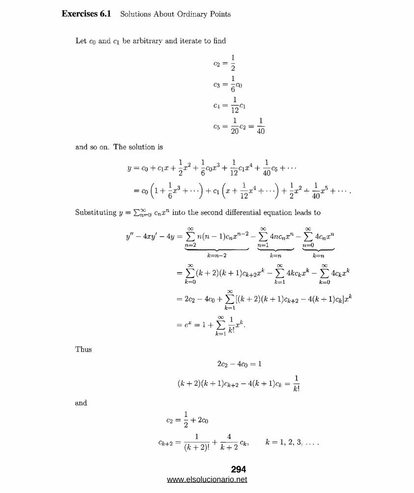
Exercises 6.1 Solutions About Ordinary Points
Let cq and ci be arbitrary and iterate to find
C2 2C3 = tQ)6
C<= 12Cl
C'5 20C2 40
and so on. The solution is1 2 1 3 1 4 1
y = c0 + c\x + -x + qCqx + ~ cix + — c5 + • • •
= C0( l + l I 3 + . . . ) + c l( I + ^ , c-1 + . . . ) + l a:2 + ^ 5 +
Substituting y = cn'xn into the second differential equation leads toOO OC o c
y" - 4xy' - 4;y = 53 »(« - l)cnxn-2 - 53 4ncnxn - 53 4cnxnn = 2 n = l n = 0s------ ------ " "--- --- ' >-- -'
k—n—2 k = n k—n
OC o c
= 5 3 0 + 2)(k + 1)ofc+2 fc - 5 1 4kckxk - 53 Ackxk fc=0 fe=l k = 0
= 2c2 - 4c0 + f ) [(k + 2) (k + l)ck+2 - 4 (k + l)c*]z*k = \
o o 1
= t
Thus
and
2c2 - 4co = 1
(k + 2) (ft — l)cj;.|_2 4{k + l)c& = —
2 — 2 + 2co
c‘ +2 = (jfcT2)T + kT 2 Ck' ,£= 1 ' 2^
294www.elsolucionario.net
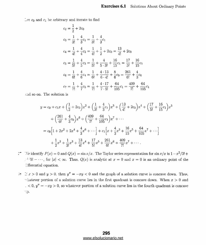
Exercises 6.1 Solutions About Ordinary Points
let co and ci bo arbitrary and iterate to find
1C2 = ^ + 2 c0
1 4 1 4
C3“ 3! + 3C l“ 3! + 3Cl
1 4 1 1 , 13
C4 = 4! + 4C2 “ 4! + 2 + 0 “ ¥ + 0
1 4 1 4 16 17 16C5 — 77 + -C3 — fT + z— 7 + ttC i — T7 + — Ci
5! o -5! 0 • 3! lo o! 15
1 4 1 4-13 8 261 4
C6 “ 6! + 6Cl _ 6! + 6^4! + 6°° “ ~Sf + 3 ^
1 4 1 4-17 64 409 64
C7 - 7! + 7C'5 - 7! + 5^5! + Ws"1 “ I T + MS*
-:id so on. The solution is
V = co + C1X + ( i + 2 m y + ( | + ic ,) * 3 + ( | + + ( i[ +
/261 4 \ 6 / 409 64 . ,
+ ( lT n i T + IM *1'* +
= CO 1 + 2x2 + 2x4 + +O
+ C164
X + — T3 + — ~7l " 15 105
x +
1 9 1 3 13 4 17 5 261 6 409 7 + 2'T' + 3Tt + 4!* + 5T + lT 'r + 1T :C +
*Ve identify P(x) = 0 and Q(.r) == siiix/x. The Taylor series representation for sin.r/$ is 1 — rr2/3! +
. ’ ''5! — • • •. for |x| < oo. Thus, Q(x) is analytic at x = 0 and x = 0 is an ordinary point of the
i.ffercntial equation.
1: x > 0 and y > 0. then y" = —xy < 0 and the graph of a solution curve is concave down. Thus,
■viiatever portion of a solution curve lies in the first quadrant is concave down. When x > 0 and
. < 0 , y" = —xy > 0, so whatever portion of a solution curve lies in the fourth quadrant is concavc
"-D.
295www.elsolucionario.net

Exercises 6.1 Solutions About Ordinary Points
39. (a) Substituting y = Y^^=q nXn into the differential equation we have
OO CK) OC'
y" + xy + y = 53 n(n ~ l)cnxn~2 + 53 ncnxn + 53 CnXnn = 2 n = l n =l} ^
k—n—2 k—n k=n
oc oc oc
= J2(k + 2)(k + l)ck+2xk + 53 kckxk + J2 ckxk k= 0 A:=l fc—0
OC= (2c2 + co) + 5 3 I(^ + 2)(fc + 1)c/-4-2 + (k + l)cfc]xfe = 0.
k= 1
Thus
and
2c2 + co = 0
(k + 2)(k + l)Q;+2 + (k 1 )c£ = 0
C2 = ~ 00
Cfc+2 = k = 1-2,3,... .
Choosing cq = 1 and c\ — 0 we find
C2 = "2
C3 = C5 = Cq = • • • = 0
l ( 104 4V 2) 22 • 2
___ L _°6 6 2-2 • 2' 23 - 3!
and so on. For cq = 0 and c\ = 1 we obtain
c2 = c4 = c6 = ■ • • = 0
Cs~ ~ 3 ~ ~3!
I f I n 1 4 - 2
05 “ “ 5^ 3' _ 5 • 3 ~ ~5T
1 / 4 - 2 n 6 - 4 - 2
°7 ~~7^~5i~^ ~ 7!
296www.elsolucionario.net
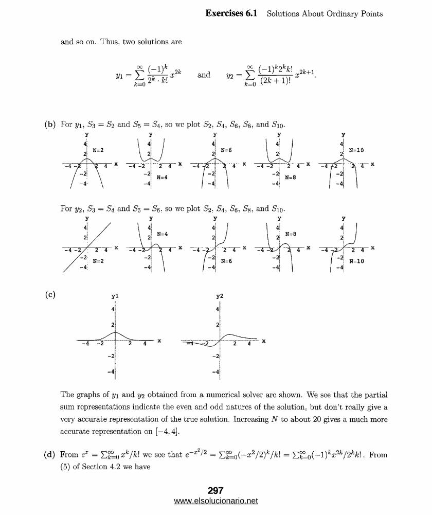
Exercises 6.1 Solutions About Ordinary Points
and so on. Thus, two solutions are
k=Q ■2k ■ kland
oc ,9Jk+1
(•>) For y\, S3 = S2 and S5 ~ S4 , so wc plot 5V S4, Sq, S&, and Siq.
The graphs of y\ and y2 obtained from a numerical solver arc shown. We see that the partial
sum representations indicate the even and odd natures of the solution, but don’t really give a
very accurate representation of the true solution. Increasing N to about 20 gives a much more
accurate representation on [—4.4].
(d) From ex — Y,bLtiXk/kl we see that e~x2/!2 ■ £j£L0(—:r2/2)fc/&! = Y3?=o(—])k3?‘k/2kk\ . From
(5) of Section 4.2 we have
297www.elsolucionario.net
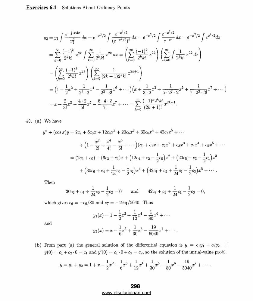
Exercises 6.1 Solutions About Ordinary Points
»- h / t * " ^ ^ f ^ =
_ y (- 1)* 2 k [ y~ _ J _ 2 t d = ( y (~1)t ( y [ — x2!-dx
~ h **« J k ^ Is 2 *« ) \ t J ,
X,2fc+li £ w ^ t ? 0 (2 ,+i»«= (1 - 5-t2 + W~2xl - P ^ 1’6 + • • ') (X + 3V + 5 ^ 2 x5 + 7 ^ 3 ! 17 + '
2 3 4-2 5 6-4-2 7 ~ (-= x - ^ + — x' - — =i~x +-" = T .T ‘ X2k+l
3!" -5! *' 7! " £To (2/c +1)!
0. (a) We have
y" + (cos x)y = 2c2 + 603,7: + 12c±x2 + 20csrr3 + 30ce^4 -t- 42c7£5 -1--
9 4
+ (1 - + j- - ^ H---) (co + CiX + C2X2 + C3Z3 + G[X4 + Cr>X5 +
= (2c2 + co) + (6C3 + ci)a? + (1204 + C2 - ^co)*2 + (20c5 + c3 - ^ci):r3
1 1 1 1 + (30ce + C4 + — cq — -C2)^4 + (42c7 + C5 + — cj — H-- •
Then
30cg + Cl + ^co - -C2 = 0 and 42c7 + eg + ^ c i - ^c3 = 0,
which gives cq = —co/80 and c7 = — 19ci/5040. Thus
i«W = i - ^ 2 + ^ 4 - ^ e + ---
and, , 1 3 1 , 19 7
■mix) = x — -x + — x — ■ -x + • • • . y w 6 30 5040
(b) From part (a) the general solution of the differential equation is y = c\y\ + 0 2 1)2 -
y(0) = ci + C2 • 0 = Ci and y’(0) = ci • 0 + C2 = C2, so the solution of the initial-value prob
www.elsolucionario.net
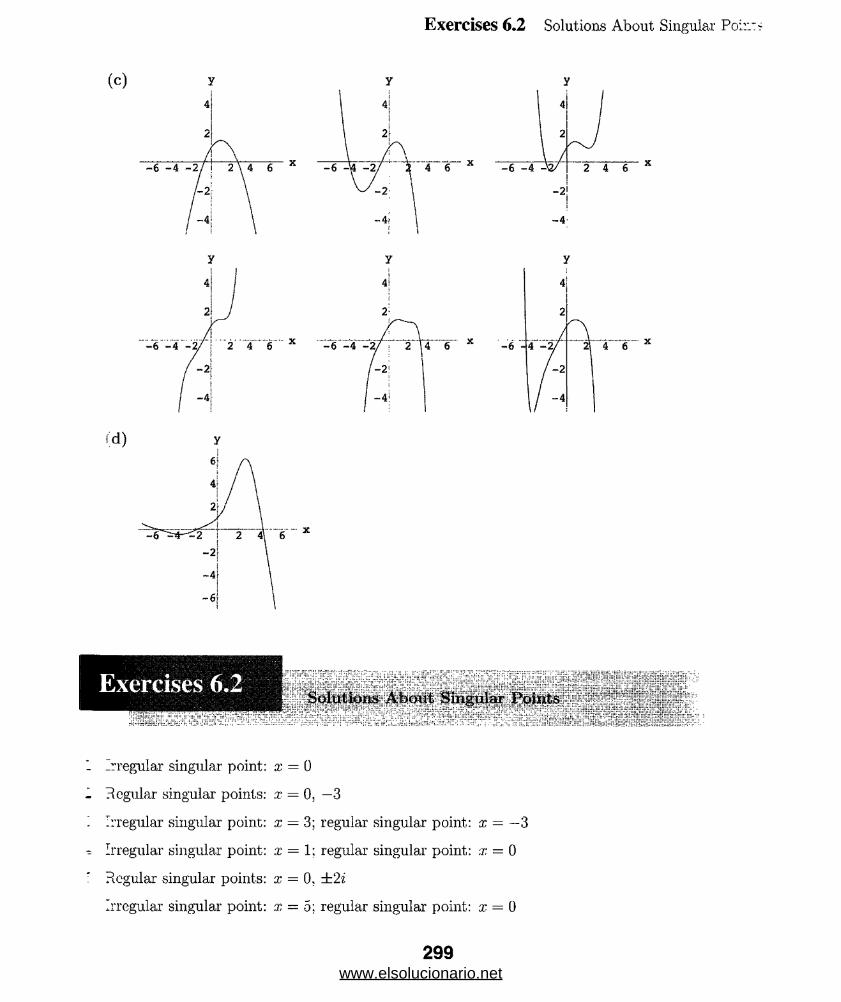
Exercises 6.2 Solutions About Singular Po::::?
fd) y
Irregular singular point: x = 0Regular singular points: x = 0 , —3Irregular singular point: x = 3; regular singular point: x = — 3Irregular singular point: x = 1: regular singular point: x = 0Regular singular points: x = 0, ± 2zIrregular singular point: x = 5 ; regular singular point: x = 0
299www.elsolucionario.net
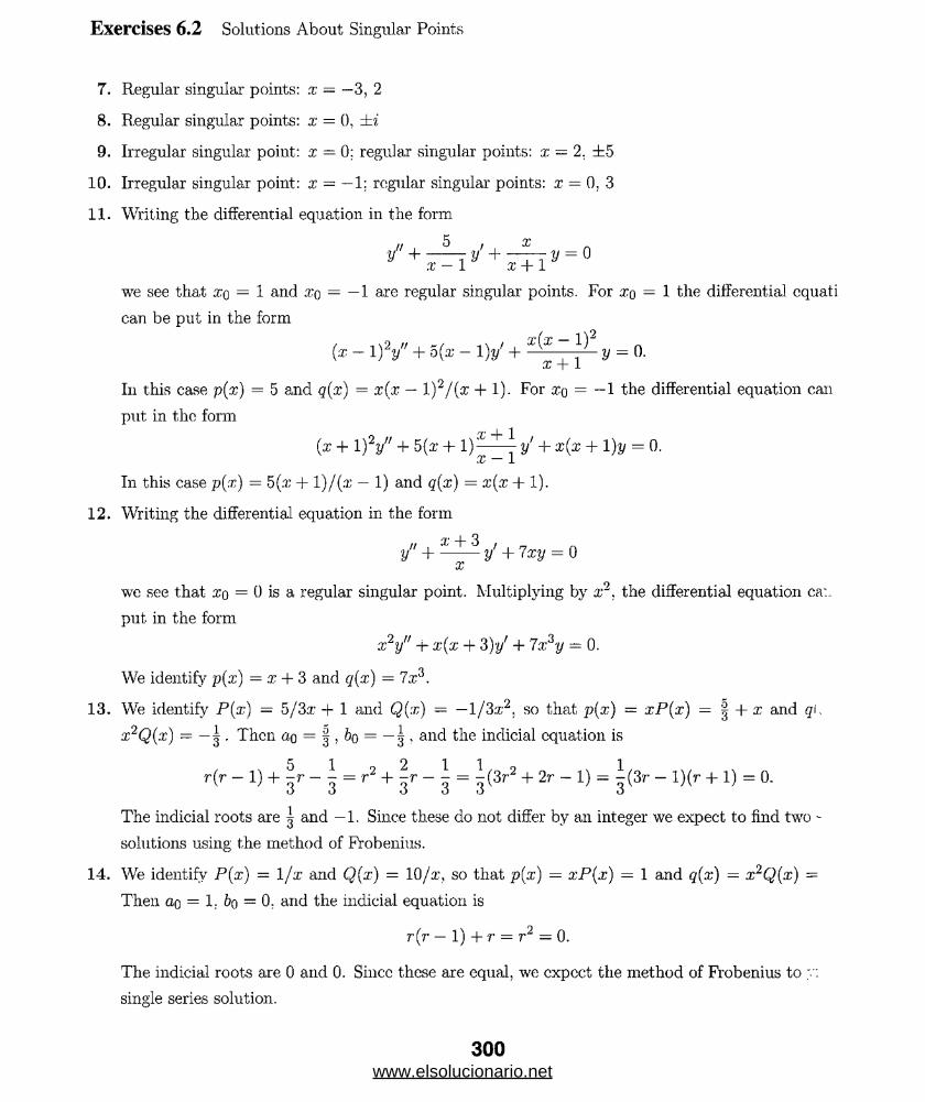
Exercises 6.2 Solutions About Singular Points
7. Regular singular points: x = —3, 2
8. Regular singular points: x = 0, ±%
9. Irregular singular point: x — 0; regular singular points: x — 2. ±5
10. Irregular singular point: x — —1; regular singular points: x = 0, 3
11. Writing the differential equation in the form
// 5 , x
* + 'J + 7 T I 'J = 0
we see that xq = 1 and xq = — 1 are regular singular points. For xo = 1 the differential cquati
can be put in the form
(x - 1)V + 5(* - IV + s(* - ' )2 y = 0.X + 1
In this case p(x) = 5 and q(x) = x(x — I )2/(x + 1). For xq = —1 the differential equation can
put in the form
(x + 1 )2y" + 5(x + 1)X + ] y' + x(x + 1 )y = 0.x — 1
In this case p(x) — 5(x + l)/(x — 1) and q(x) = x(x + 1).
12. Writing the differential equation in the form
y" + y' + 7 xy = 0x
we see that xo = 0 is a regular singular point. Multiplying by x2. the differential equation ca:.
put in the form
x2y" + x(x + 3 )y' + 7x3y — 0.
We identify p(x) = x + 3 and q[x) = 7x3.
13. We identify P(x) ~ -5/3x + 1 and Q(x) = —l/3x2, so that p(x) = xP(x) = | + x and q\.
x2Q(x) = — g • Then ao = | , bo = — | , and the indicial equation is
r(r _ 1) + _ I = r 2 + _ I = i ( 3r2 + 2r - 1) = ^(3r - l)(r + 1) = 0 .The indicial roots are j and —1. Since these do not differ by an integer we expect to find two -
solutions using the method of Frobenius.
14. We identify P(x) = 1/x and Q(x) = 10/x, so that p(x) = xP(x) = 1 and <?(x) = x2Q(x) =
Then ao = 1- bo = 0. and the indicial equation is
r(r — 1) + r = r2 = 0 .The indicial roots are 0 and 0. Since these are equal, we cxpect the method of Frobenius to y:
single series solution.
300www.elsolucionario.net
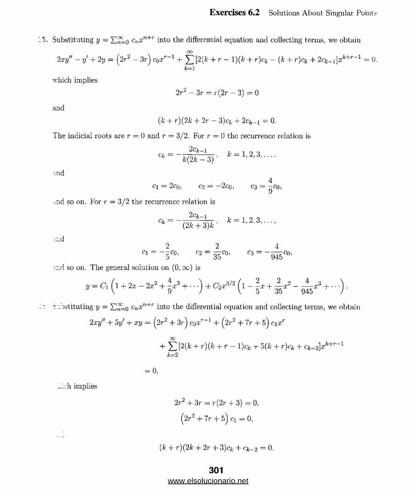
Exercises 6.2 Solutions About Singular Point?
Substituting y — cnxn+r into the differential equation and collecting terms, we obtain
OO
2xy" - y' + 2y = (2r2 - 3r) c0:r'r_1 + 53l2(*' + r ~ l )(k + r)ck - (k + r)ck + 2cfc_1]xfc+r_i = 0.fc=i
which implies
2r2 - 3r = r(2r - 3) = 0
and
(k + r) (2 k + 2r — 3 )ck + 2c£—i = 0.
The indicial roots are r = 0 and r = 3/2. For r = 0 the recurrence relation is
_ 2Cfc_i
C,!_ k(2k~3)'-
-.nd4
Cl = 2C(). C2 = —2co, C3 = -Co,
.-.nd so on. For r = 3/2 the recurrence relation is
:-.::d
Ci = - i 00’ C2 = 1 " ° ’ c» = “ d s ’’'0’
-„:.d so on. The general solution on (0, oo) is
4Vr.ibstituting y — en.xn+r into the differential equation and collecting terms, we obtain
2xy" + 5y' -r xy = (2r2 + 3r) cq.t7'-1 + (2r2 + 7r + -5j ci:rr
OC
+ 53[2(fc + r){k + r - 1 )ck -r 5(k + r)ck + ck-2]xk+r 1 k=2
—i ch implies
2r2 + 3r = r(2r + 3) = 0,
(2r2 + 7r + 5) a = 0,
(k + r)(2k + 2 r + 3 )ck + cfc_2 = 0.
301www.elsolucionario.net
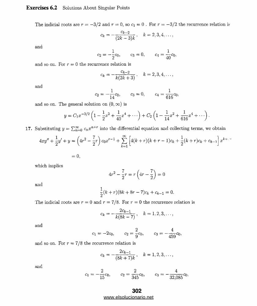
Exercises 6.2 Solutions About Singular Points
The indicial roots axe r — — 3/2 and r = 0, so c\= 0 . For r = —3/2 the recurrence relation i
Ck-2
(2k - 3)k k = 2.3A.and
1 n 1 C 2 = - p C Q , C * 3 = 0 , C l = — C o ;
and so oil. For r = 0 the recurrence relation is
Cfc-2
k(2k + 3). k = 2 ,3 ,4 ,...,
and
C2 = “ 77c0: C3 = 0. C4 = 7^7 Co;14 616
and so on. The general solution on (0, oo) is
v = Cyx-V* ( l - i * 2 + + . . . ) + C2 ( l - + J j x * + . . . ) .
17. Substituting y = cn..xn4"'r into the differential equation and collecting terms, we obtain
oci / 7 \ . 00 r i4 ^ / + + V = ( 4r2 - - r ) c0xr~1 + ]T 4(fc + r)(k + r - 1 )ck + -(k + r)ck + c*_i
fc=ia;
= 0,
which implies
and
4r* _ r — r { 4r _ ] — o
-(k + r)(Sk + 8r - 7)ck + ck-i = 0.
The indicial roots are r = 0 and r = 7/8. For r = 0 the recurrence relation is
2cfc-iCfc =
fc(8fc - 7)k = 1.2 ,3 , . . . ,
and
ci = -2co,
and so on. For r = 7/8 the recurrence relation is
Co,
www.elsolucionario.net
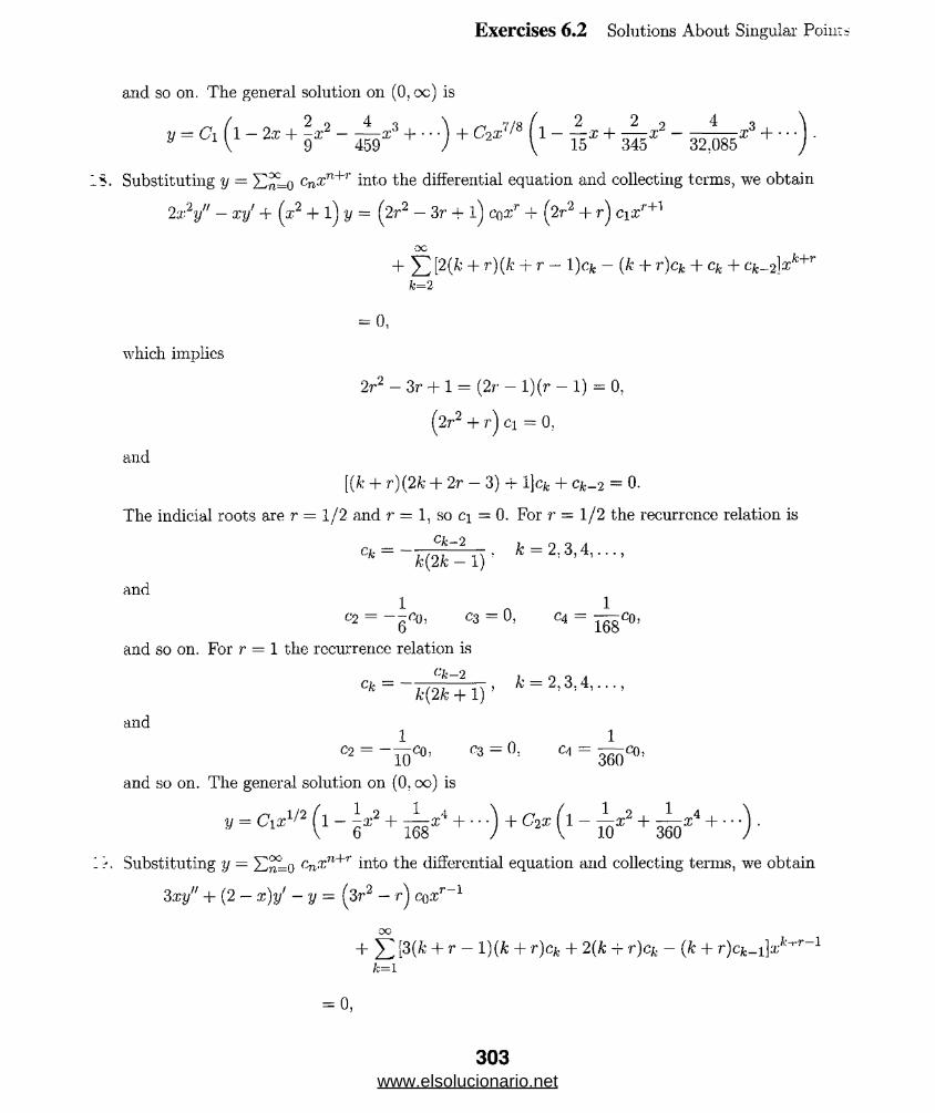
Exercises 6.2 Solutions About Singular Point;
and so on. The general solution on (0, oc) is
9 = C1 ( l- 2 ^ + ^ 2- ^ + . . ) + C 2 8 ( l - | ;C + s| x 2- i ^ x 3 +
IS. Substituting y = 2Zj£=o Cn%n+r into the differential equation and collecting terms, we obtain 2x2y" — xy' + (z2 + l) y = (2r2 — 3r + l) cqxt 4- (2r1 + r) c\xr+1
+ Y [2 (fc + r)(k + r - l)cfc - (fc + r)ck + ck + ck- 2}% k=2
fc+r
= o,
which implies2 r2 — 3r + 1 = (2 r — l)(i— 1) = 0,
(2r2 + r) ci = 0,
and[(k + r)(2k + 2r - 3) + 1 }ck + ck-2 = 0.
The indicial roots are r = 1/2 and r = 1, so ci = 0. For r = 1/2 the recurrence relation is* = y *= 2 .3 .^ .- - .
and1 n 1
c2 = —pQ), C3 = 0, C4 — -r zCO,6 168
and so on. For r = 1 the recurrence relation is
andC2 = -^C0, CS = 0, ^ = 3 0,
and so on. The general solution on (0,00) isy = ClX' » ( l - ix-2 + 4 ' 4 + " ') + ( J - ^ + 3 4 + " ' ) '
1 Substituting y = cnxn+T into the differential equation and collecting terms, we obtain3xy" + (2 - x)t/ - y = (3r2 - r) c\yxr~1
+ Y (3(fe + r - l) ( k + r)ck + 2(k + r)ck - (k + r)cfc_ i]x"1 ’ fc=i
fr-rJ-1
= 0,
303www.elsolucionario.net

Exercises 6.2 Solutions About Singular Points
which implies
and
3 r'2 — r = r(3r — 1) = 0
(k + r)(3k + 3r - 1 )ck - (k + r)ck_i = 0.
The indicial roots arc r = 0 and r = 1/3. For r = 0 the recurrence relation is
CkQfc-i
3k — 1k = 1 ,2 ,3 ,...,
and
ci = -cq. C2 = - c o ,
and so on. For r = 1/3 the recurrence relation is
and
ci = ^ cq, C3 162co,1 1 13C0, C, = - C Q ,
and so on. The general solution on (0. oc) is
» = c1(i + 5 * + + + -) + c l/3(i + i:c + Bl 2 + ikI, + -)-20. Substituting y = cnxn+r into the differential equation and collecting terms, we obtain
x2y" - (x - - )y = [ r
= 0,
which implies
and
2 \ 00 r 22 - r + - ) c.q x t + J2 (k + r)(k + r - 1 )c& + ^ ck - c*_i
r2 _ r + i = ( , . _ | ) ( r _ i ) = 0
X,/c-hr
(k + r)(k + r — 1) + - Ck ~ Ck-1 = 0.
The indicial roots are r = 2/3 and r = 1/3. For r — 2/3 the recurrence relation is
3cfc_ i
and
Ck. =
Cl = |Cq ,
3 k2 + k, k = 1 ,2 ,3 ,...,
9
C2 = 56°"’ C3 560Q)’
and so on. For r = 1/3 the recurrence relation is
3cfc_iCk =
3 k2 — k, k — 1 ,2 ,3 ,...,
304www.elsolucionario.net
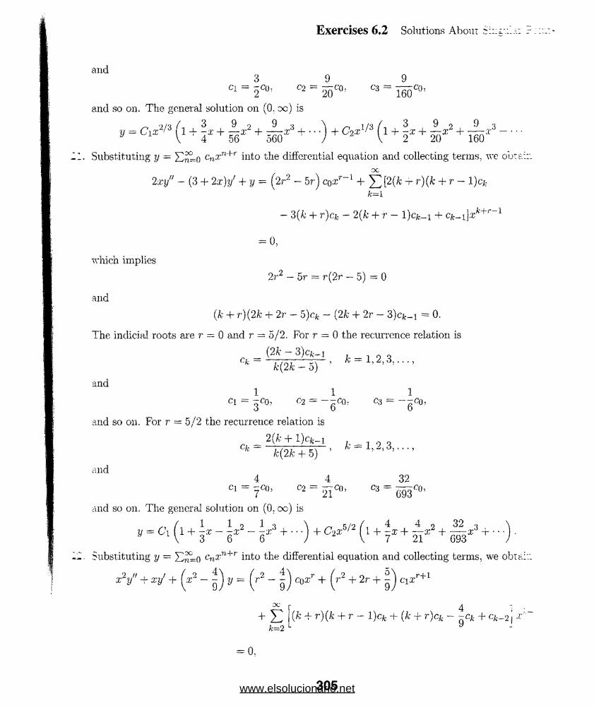
Exercises 6.2 Solutions About
and
C1 = 2°“’ C2 = 20CO' C3 = 160°°’
and so on. The general solution on (0. oc) is
, = C ^ '3 (l + \t + | * 2 + ^ + . . . )+ C2*>/3 (l + §x + | * 2 + JL* - ■Substituting y = cnxn+r into the differential equation and collecting terms, we ob
•OC
2xy" - (3 + 2x)y' + y = (2r2 - 5rj c0xr~l -f 5^[2(ft -h r)(k + r - l)ckk=i
- 3(ft + r)ck - 2(ft + r - l)cfc_ i + cfc_ 1]:rA'+r_1
= 0,which implies
and
2r2 - 5r = r(2r - 5) = 0
(ft + r)(2ft + 2r - 5)c* - (2ft + 2r - 3)c*_i = 0.
The indicial roots are r = 0 and r = 5/2. For r = 0 the recurrence relation is
r _ (2 ft 3)cfc_i 12 3ft(2ft — 5) !
and
ci ■ -co, C-2 = -rQ): C3 == --co,3 6 6
and so on. For r = i5/2 the recurrence relation is
2(ft + l)c*;_cjb =
and
. _ 2(ft + i;cfc_i , _ 7 9 „
* k(2k + 5) ’
Cl = C2 = - c , C3 = — op,39
! = 7 ^ c0> c3 =
and so on. The general solution on (0. oo) is
\ „ q/9 4 4 o 32: Xy = C\ ( l + \x - \x2 - -i-- ) + C‘2 Xbf2 f 1 + ^x + ^-x2 + ^ ~’5 '
3" 6 6 ) - \ 7 21" 693
Substituting y = c„.a-rH‘r into the differential equation and collecting terms, we ob
x2y" + xy' + (x2 ~ ^ j y = (V2 - ^ j coxr + (r2 + 2r + 0 cia.,r+1
+ J2 ik + T)(k + r ~ + (k + r)ck ~ Qck + Ck-2 | k~2 L y
= 0 .
305www.elsolucionario.net

Exercises 6.2 Solutions About Singular Points
which implies
r2 - 5 =(r+D(r-!)=o’r2 + 2r + - ) Cl = 0,
and
(k + r)2 -9J
Ck + Ck-2 = 0.
The indicial roots arc r = —2/3 and r = 2/3, so c\ = 0. For r = —2/3 the recurrence relation >
9c/c-2
; 4)
and3 ^ 9
C2 = — C3 - 0; C4 = yTjgCOj
and so on. For r = 2/3 the recurrence relation is
9Cfc-2
" 3k(3k + 4)Ck /c = 2.3,4.......
and
6'2 = “ Sj"0’ C3 = ° ’ C4 = d i o " 0’and so on. The general solution on (0, oc) is
* - ( ' ~ r 2+ i s * ‘ + - ) + c - 2/31 1 - 1 * 2+ m **+ ■ •) ■•
23. Substituting y = I^Lo cn^rt+r into the differential equation and collecting terms, we obtain
9x2y" + 9x2y' + 2y — (9r2 — 9r + 2) coxr
+ £ + r)(^ + r ~ l) cfc + 2ck + 9(fc + r — l)ct_i]xfc+r fc=i
= 0,
which implies
and
9r2 — 9r + 2 = (3r — l)(3r — 2) = 0
[9(k + r)(k — r - 1) + 2]ck + 9(k + r - l)cfc_i = 0.
The indicial roots are r = 1/3 and r = 2/3. For r = 1/3 the recurrence relation is
(3A - 2)e*_1ck —
k(3k - 1), k — 1,2,3,
306www.elsolucionario.net
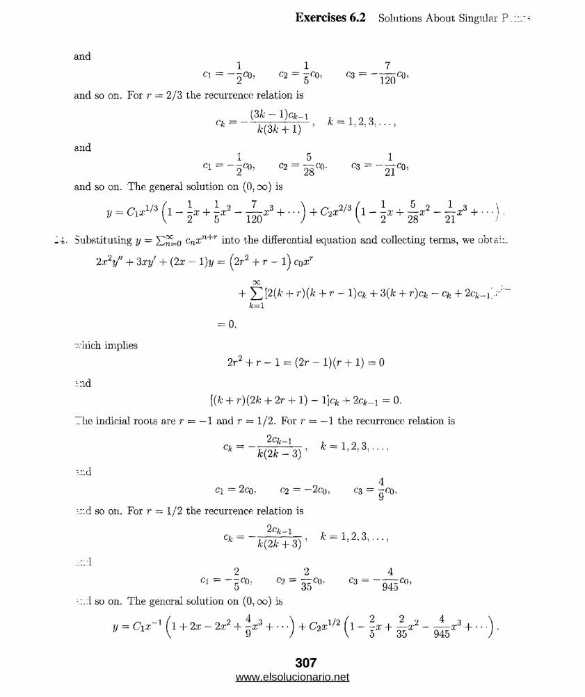
Exercises 6.2 Solutions About Singular P.i:.:-
Cl = “I <So’ C2 = r ° ’ C3 = ' I S " 0'
and so on. For r = 2/3 the recurrence relation is
(3fc - l)cfc_i
t(3fc + l) ’
and
and
ci - — ttCo, c2 = — co- c3 = - — co,2 - 28 ° 21
and so on. The general solution on (0, oo) is
= c,***fl - l-t + - tL*3 + ...UC*&*(l-i* + - i*3 +?y V 2~ ' 5" 120" ' J ' V 2" ' 28” 21
-4 . Substituting y = cnxn+r into the differential equation and collecting terms, we obtai:.
2:r2y" -f 3;r*/ + (2x — 1 )y = ^2r2 + r — l) co.xr
OC
+ 5 3 l2(fc + r ) ( k + r _ + 3(fc + r )c^ - Cfc + 2cjt_i;.r'- fc=l
= 0,■vhich implies
2r2 + r - 1 = (2r - l)(r + 1) = 0.^d
[(& + v){2k + 2r + l) — ljCfc -j- 2cfc__i = 0.
The indicial roots are r = — 1 and r = 1/2. For r = — 1 the recurrence relation is
C* = ~ k(2k — 3) 5 * = 1’2>3’ ---
\r_d4
ci - 2co; C2 = — 2co, C3 = —r?o,
d so on. For r = 1/2 the recurrence relation is
Cfc = ~k(2k + 3) : fe=1>2’3*--*’
2 2 4Cl = “ CO; C2 = — Co- C3 = - — Co,
5 3o 94o
::.i so on. The general solution on (0, oo) is
y = Ci;r_1 f 1 + 2x - 2a;2 + ^a:3 H-- ) + C2a;1/2 f l - ~ +\ 9 / V 0 35 94-5
307www.elsolucionario.net

25. Substituting y = cn%n+r into the differential equation and collecting terms, we obtain
xy" + 2y' — xy = (r2 + r) coX'r_1 + (r2 -1- 3r + c\xr
Exercises 6.2 Solutions About Singular Points
+ Y P + rKk + r “ iJcjfe + 2(k + r)°k - Ck-2]x k—2
k-rr—1
= o,
which implies
r2 + r = r(r +1) = 0.
(r2 + 3r + 2) c\ — 0,
and
(fc + r)(k + r + 1 )ck - cfc_2 = 0.
The indicial roots are r\ = 0 and r2 = —1, so c\ — 0. For r\ — 0 the recurrence relation is
and
k = 2 ’ ^
°2 = 2[Co
C3 = Co — C7 = • • • = 0
1C4 — —.CQ
o!
C2n ~ (2n + l) !Co'
For r‘2 = — 1 the recurrence relation is
www.elsolucionario.net

The general solution 011 (0.00) is
1
x
1
oc 1
,t=6(2n + i)! + C2 Z1 .,2/;
r^(2™)f
= — [Ci sinh x + C2 cosh a:].x
. Substituting y = Y1 =q cnxn+r into the differential equation and collecting terms, we obte.::
2„// _i_ _i_ ( ,, _ f r2 _ C();rr _j_ fr2 + 2r + 7^ ci2'r+1x*y" + xy' + ( x- - - ) y
which implies
and
X r 1+ Y , (k + r)(ft + r - 1 )ck + (ft + r)ck - -ck + ck._2 .r
fc=2 L= 0,
r2 “ s = (r“§)(r+i ,=0’r2 + 2r-h 0 ci = 0,
(ft + r f - Ck + ck-2 — 0.
The indicial roots are r\ = 1/2 and r2 = —1/2, so ci — 0. For ri = 1/2 the recurrence relat
Cfc-2
and
C4 = ^ 0
(_l)n c2n = ,n__ , -mQ)-
(2n + 1)!
For T'2 = —1/2 the recurrence relation is
ck — ~TTT~~7\ ’ ft = 2,3,4,.ft(fc - 1)
309
www.elsolucionario.net

Exercises 6.2 Solutions About Singular Points
and
C2 = -yCQ
C3 = Cg = Cf = • ■ • = 0
C4 =
—(-1)"(2n)!
C o -
The general solution on (0, oc) is
V = £(- 1)"
(2« +1)!
oc /_i\ n
= CiT-1/2 V __1 k c n + iy.
X2n + C 2Z-l/ 2 £(- d >
n=0 (2^ )!
*2”+i + C2*-1/2£( - ! ) * >
(2w)!
= x~1/2 [Ci sin x + C2 cos :r].
27. Substituting y = cn^n+r into the differential equation and collecting terms, we obtain
OC
x y " - x y ' + y = ( r 2 - r) Co;cr_1 + £ ] [(k + r + 1 )(fc + r ) c *:+1 - (fc + r ) c k + c k] x k + r = 0
which implies
k=0
r 2 — r = r ( r — 1 ) = 0
and
(k + r + l)(k -j- r)cfc-|-i — (k + r — l)c& = 0.
The indicial roots are r\ = 1 and t 2 = 0. For ri = 1 the recurrence relation is
kck
Ck+1 (k + 2){k + l )
and one solution is y \ = cq x . A second solution is
- J - l d x
, * = 0 ,1 ,2 ,...,
y2 = xJ 2 --dx = XJ 2 dx = xj 2 + x + \x* + ’ ’) dxr ( 1 1 1 1 1 9
= X j ( — H---------h - + 7Tix + — X" -f------- ) d x = Xx 2 x 2 3! 4!
x ia x - i + l xi + ± x* + ± x*
1 9 1 3 + In x — —x + — x" + — x +1
2* 12 72
The general solution on (0, oc) is
y = Cix + C2y2 {x).
310www.elsolucionario.net

Substituting y = X T=o cn^,n+r into the differential equation and collecting terms, we obtain
y" -f —y' — 2y = (V2 + 2r) cor/;7 _2 + (r2 + 4r + 3) C]_xr~1
OC-
+ S P + r)(fc + 7’ - + 3(fc + r)cfc - 2cfe—2]5c*'*"r“2k=2
Exercises 6.2 Solutions A .'. :.- S :
= 0,
“'liich implies
r2 + 2r = r(r + 2) = 0
(r2 + 4r + 3) cj = 0
(k + r)(A' -+■ t + 2)ck — 2c^_2 = 0.
riie indicial roots are ri = 0 and r?. = —2, so ci ~ 0. For ri = 0 the recurrence relation is
2Cfe-2c-k =
k ( k -|- 2), A: = 2,3,4.
C2 = -gCo
C3 = C5 = C7 = • • • = 0
C4 = 48 C°
<‘61.152
Cq-
"_1t result is
ircond solution is
/■ e~ f (3 / x )d x dx
f I f -i 1 9 ^ 4 6 \= " J *T(T+Jx~+ A 4 ‘ / 3 (* " r + 48" + 57<f +-J■)
I / 1 1 7 19 3 i ,= y i l { J j - T X + T&X -576X +■"]<** = !«
1 M n r + V 19 ,r ^~~ 2a^ _ 2 96 _ 2^04i T
= “ 2^11 w + y1 7 2 19 4-a + - rrz^x +
2a:2 96' 2.304
311www.elsolucionario.net

y = Ciy](x) + Ckwix).
29. Substituting y = cnxn+r into the differential equation and collecting terms, we obtain
Exercises 6.2 Solutions About Singular Points
The general solution on (0. oo) is
xy11 + (1 - x)y - y = r2c0xr 1 + [(A: + r)(k + r - 1 )ck + (k + r)ck - (k + r)c*_i]x';,—i
which implies r2 — 0 and
(k + r)2cfr - {k + r)ck-i = 0.
The indicial roots are n = = 0 and the recurrence relation is
<* = -y 1 , fc = 1,2,3.......k
fc+r—1
One solution is
Vi = cq (1 + x + -x + H-- ) — (%ex.
A second solution is
- f ( l / x - l ) d x f e T . / x . 1 ^
S/2 = V i J --- ----- dx = e J -jSrdx = e J xe dx
da;
- e* I In x — re + - g T g j Z 3 + • • • = e* In x - ex £00 f _]_)«+1
n • n!. *“■n = l
The general solution on (0, oo) is
4- d o t * ( In r - V {n • tt!
l_1 VH-1 >
ln ;r- E 3;nn= l
30. Substituting y — cnxn+r into the differential equation and collecting terms, we obtain
OC
xy" + y' + y = ■r2coxr~1 + [(& + r)(k + r - l) cfc + (* + r)ck + cfc-i]xfc+r_:l = 0*=i
which implies r2 = 0 and
(k + r )2cj~ + Ck-i = 0.
The indicial roots are ri = = 0 and the recurrence relation is
* = 1,2,3,
One solution is
www.elsolucionario.net

Exercises 6.2
■ /(l/.E)<£rdx = vt I —
dx
A sccond solution is
/• e' J ' f a.ry-2 = y\ / --------2— dx = vi / —------------ ;----------:---------------5
' x f 1 — ;r + i r 2 —
^ x ( l — 2x + if.r2 — |;r3 + ^ . r ’1 — • • •)
f 1 /, n 5 o 23 .. 677 4 \ ,= y iJ - ( l + 2x + -x + T *-+ 288* + " 7 dT
y/1 5 23 <) 677 3 \ ,
= n j { * + 2 + 2x + -93r + ™ * + '- ')d*
= yi5 9 23 3 677 4
lna: + 2x + -ar + — x’ + j j ^ x + ■
* ^ 2 , 23 3 , 6 7 7 4= yi In x + yi ^2a; + -x + — x* + 3^52 + ‘ " ) ‘
The general solution 011 (0. oc) is
V = Ciyi{x) + C2?/2(*)-
Substituting y = SjSzO c«rr”’+r i110 the differential equation and collecting terms, we obtaii.
OOxy" + (x - 6)y' - 3y = (r1 - 7r)co.xr_1 + ^ [(A- + r)(A~ -f- r - l)cA; -f- (k + r - 1 )q._:
fe=i
- 6(fc + r)cfc - 3c&_ 1]x-fc+r"~1 = 0,
which implies
r2 - 7 r = r(r - 7) = 0
and
(fc + r)(Ai + r - 7)c* + (A- + r - 4)c*_i = 0.
The indicial roots are ri = 7 and ro — 0. For ri = 7 the recurrence relation is
(A* -j- ()kc,k -r (fc + 3)c£_i = 0, /c — 1,2 ,3 ,... ,or
Ck = ~ W V T )ct~1' k = 1’2’3’ - --
313www.elsolucionario.net
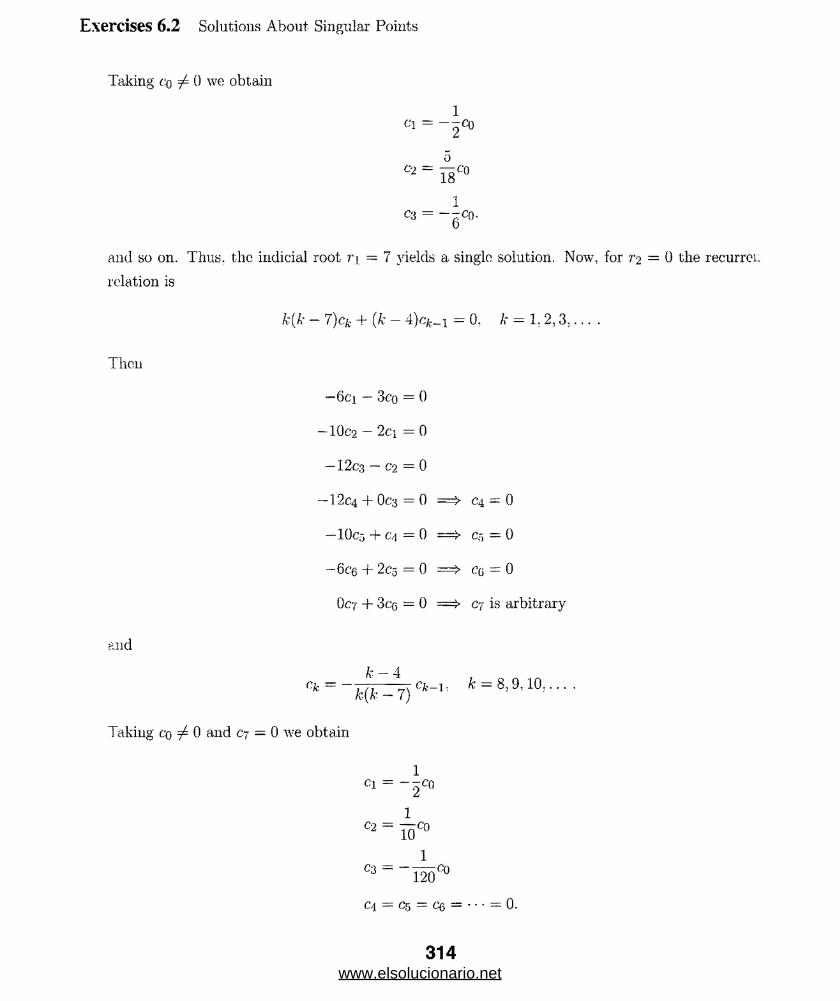
Exercises 6.2 Solutions About Singular Points
Taking cq 7 0 we obtain
ci = --co
C‘) = — Cn 18 U
C3 = — 77CO.6
and so on. Thus, the indicial root r\ = 7 yields a single solution. Now, for = 0 the recurrci:
relation is
- 7)ck + (k - 4)cfc_x =0 , k = 1 ,2 ,3 ,....
Then
and
—6ci — 3co = 0
-10C2 - 2a = 0
— 12C3 — C‘2 = 0
-12C4 + 0C3 = 0 = * C4 = 0— IOC5 "I” C.'l : 0 Cg = 0
—6cg + 2co - 0 Co = 0
Oct + 3q> = 0 ==>■ C7 is arbitrary
c t = ~ k ( r = j ) c t - ' ’ * - 8 - 9 - 1 0 -
Taking cq 7 0 and 07 = 0 we obtain
1
1<
1
2(
c-4 = c5 = ce = ■ ■ ■ = 0.314
Cl = - - c o
<S = i5<*
www.elsolucionario.net

Exercises 6.2 Solutions About Singular P. in
ci = 02 = Oi = C4 = C5 = Cq = 0
C8 = ~\c,
Taking co = 0 and c? 7 0 we obtain
C 9= 36°7
do = - 3JO7,
and so on. In this case wc obtain the two solutions
Vl — 1 — + ~ x 2 — — x3 and y2 = x' — ^or8 + ~ x 9 — -^zX10 -- .y 2 10 120 ,y 2 36 36
12. Substituting y = cn 'n+r into the differential equation and collecting terms, we obta:
x(x - l)y" + 3?/ - 2y
OC
— ^4r _ coXr~ L + £ [(ft + r - l)(k + r — 12)cjt_i - (ft + r)(k. + r —fc=1
+ 3(k + r)cf. ■ 2c^_i]a:A' ' r 1
= 0,
viiich implies
and
4 r — r1 = r( 4 — r) = 0
—(Ar + r)(ft + t — 4)ck + [(A; + r — l)(ft + r — 2) — 2]c£_ 1 — 0.
The indicial roots are r\— A and r2 = 0. For ri = 4 the recurrence relation is
— (ft + 4) Are*; + [(ft -i- 3)(ft + 2 ) — 2 ]c ^ _ i = 0
or
Taking co 7 0 we obtain
Ofc = — 7— C jfc-i, ft = 1 ,2 .3 ,... .
ci 2co
c2 ~ 3c0
C3 = 4c0;
315www.elsolucionario.net
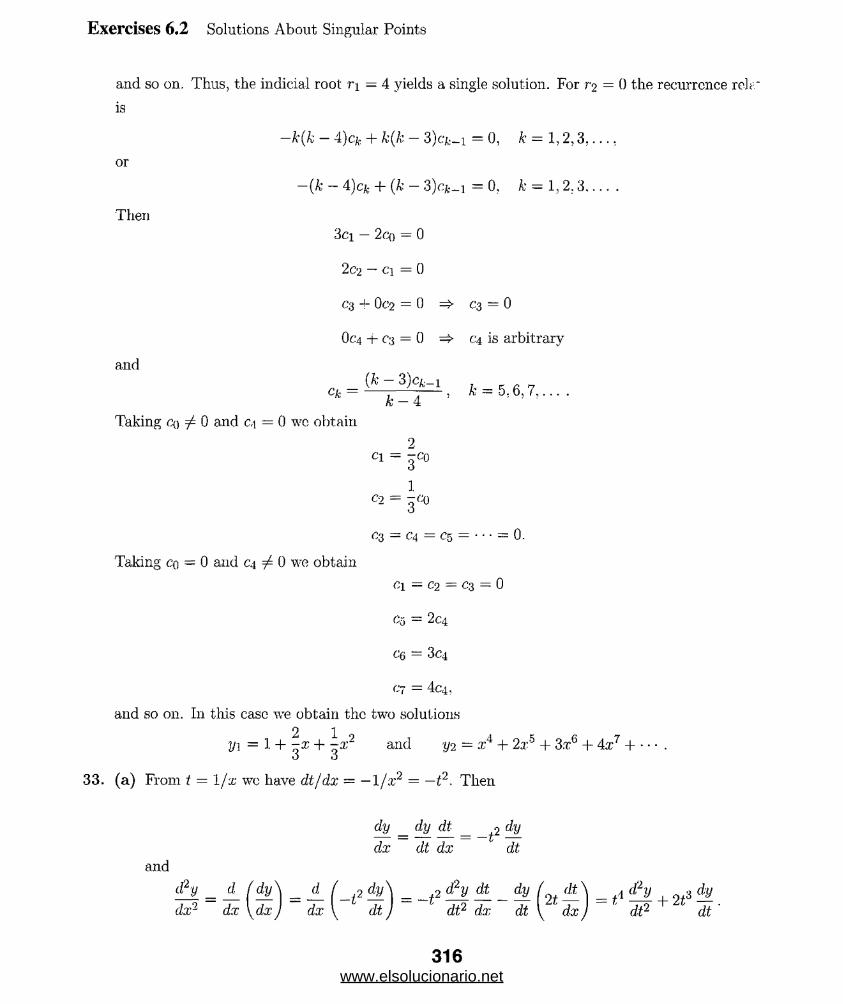
Exercises 6.2 Solutions About Singular Points
and so on. Thus, the indicial root ri = 4 yields a single solution. For r? = 0 the recurrence relt
is
—k(k — 4)c/p + k(k, — 3)ck_i = 0, k — 1 ,2 ,3 ,...,
—(k — 4)cft (k — = 0, k = 1 ,2 .3 .... .
or
Then
and
3 c i — 2 c q = 0
2c2 - c i = 0
C3 H- 0c‘2 = 0 =£• C3 = 0
Oc‘4 + C3 = 0 =i> c-4 is arbitrary
ct = (* 7 % -‘ , * - 5 ,6 ,7 ,. .. .k-A
Taking co 7 0 and c.\ = 0 we obtain
2ci = -co
1C2 = 3C0
c/i = ('4 = C5 = • • • = 0.
Taking cq = 0 and C4 / 0 we obtain
Cl = C2 = C3 - 0
Co = 2 c4
Cq = 3C4
c- = 4c4,
and so on. In this case we obtain the two solutions
2 1yi = 1 + -x + -x2 and y% = x4 + 2xa + 3rc6 + Ax7 +
33. (a) From t = 1/x we have dt/dx = — 1/x2 = —t2. Then
and
dy _ dy dt ^ dy
dx dt dx dt
ify _d_ ( dy\ _d_ / 2 dy\ = 2 Sy dt _ dy f dt\ _\&y_ 9 3 dJ l
dx1 dx I dx) dx I d t) dt2 dx dt \ dx) dt2 dt
316www.elsolucionario.net
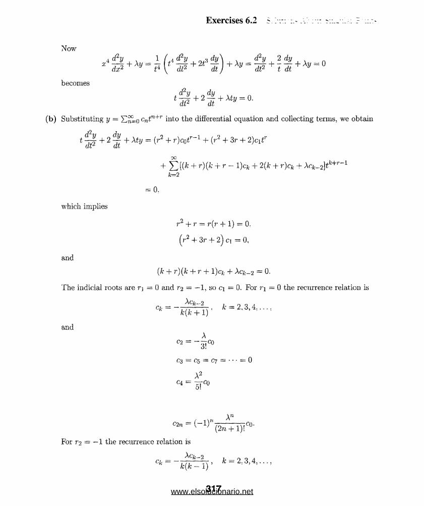
Now
Exercises 6.2
4 d2y . \ 1 (ri d<2y 10+3 dv\ , * _ d2y , 2dy , \ _ n1 d7‘ +Xy~ ¥ * d f i+2t d i ) +Xy~ W + ~tdi.+Xy~ 0
becomes
(b) Substituting y = SjJLo cntn+r into the differential equation and collecting terms, we obtain
t + 2 -rjj; + Aty = (r2 + ?’)c(jtr 1 + (•/•“ + 3r 4- 2)ci£r
+ 1( + ' )(A- -i- r — l)c-fc + 2(k + r)cfc + Aq._2]*'’’H k=2
k~\-v—1
= 0.
which implies
r2 + r = r(r -f 1) = 0.
(r2 + 3r + 2) d = 0,
and
(k + r)(fc -+- r + 1) Cfc + Ac^_2 — 0.
The indicial roots are rj = 0 and r2 = — 1, so c\ = 0. For r\ - 0 the recurrence relation is
°k = ~k{k+\) ‘ fc = 2’3*4*---
andA
c2 = - ^c °
3 = C5 = c7 = ' • • = 0
A2C4 = ttCq
0!
\n
C2n= (- 1 )” ( 5 m ) ! <:o'
For r2 = — 1 the recurrence relation is
317www.elsolucionario.net

Exercises 6.2 Solutions About Singular Points
(
34. (.
andA
02 = -jjCD
03 = C5 = C7 = • • • = 0
A2C4 =
The general solution on (0, oo) is
v ( t ) = C 1 5 (£^('/It)2”+C2rl S w (Vl‘)!'
= -[Ci sinVXt + C2 C0sVAt].
z) Using t — 1/a;, the solution of the original equation is
y(x) = CiX sin + Cox cosx x
ji) Prom the boundary conditions y(a) = 0, y(b) = 0 we find
„ . V a „ VaCi sin--- h Co. cos — = 0
a a
„ . V\ vx .Ci sm —— I- C2 cos = 0.
b b
Since this is a homogeneous system of linear equations, it will have nontrivial solutions for
and C2 if
. V a V asm — cos —
a a
V a Vasm cos ——
0 b
. Va Va Va . Vasin--cos —---cos---sm ——
a b a b
. ( Va VA\ . ( r-b-a= 0.
318www.elsolucionario.net

Exercises 6.2 Solutions About Singular Points
This will be the case if
or
or. if
An —
/— mccib rnrab ,v A = ;---= ——- . n = 1, 2,
b — a L
•n27r2a262 Pnb4
L2 E l '
The critical loads arc then Pn = n2w2{a/b)2EIo jT?. Using C2 — — C\ sin(\/A/a)/cos(\/A/«)
we have. v f t s i n ( \ / A / a ) a/ A '
y = Cia; sm - cosyr—‘ VV-ZO£ cos (v A/a) ^
= C3/
= C3X sin a/A ( — — ,
Va Va Vx . >/asm — cos----cos — sm---
x a x a
x a
and
yn(x) = Csx sinnnab / I 1 \ . rnrab (a \ . mrab /\ a= C 3 X S ill — — ( -------1 J = C 4 X sm — ;— I 1
L \x a La \x
b) When n = 1, b = 11, and a = 1, we have, for
C4 = 1,
yi(x) = resin I.Itt (\ — —\ x
T.. express the differential equation in standard form:
y’" + P(x)y" + Q(x)y‘ + R(x)y = 0.
r.;pposc xq is a singular point of the differential equation. Then we say that :ro is a regular singular
■ ylnt if ( x — x q ) P ( x ), (x — xq) 2Q ( x ), and (x — .ro)'!i? ( .r ) are analytic at x = x q .>. v.:bstituting y — Y^=o cn^n^ r into the first differential equation and collecting terms, we obtain
x^y" + y = c\)XT + 53 [CA: + {k + r ~ !)(& + r ~ 2)ck. 1]xk+i = 0. fe=i
1: follows that co = 0 and
Ck = -(* + r - l)(k + r - 2)cfc_i.
T’.-.o only solution we obtain is y(x) = 0.
restituting y — H ^ - q cnxn+r into the second differential equation and collecting terms, we obtain
x2y" + (3x - l);i/ +y = -rco + 53[(* + r + l f ck ~(k + r +k—0
xk+r = 0 .
319www.elsolucionario.net

Exercises 6.2 Solutions About Singular Points
which implies
—rco = 0
(k + r + 1 )2ck — (k + r + l)cfc+1 = 0.
If co = 0. then the solution of the differential equation is y = 0. Thus, we take r = 0. from wh:
wo obtain
cfc+i = (k + A- = 0. 1. 2. ... .
Letting cq = 1 we get ci = 2. c2 = 3!. C3 = 4!, and so 011. The solution of the differential equat:
is then y = X)^=o(' + l)!xn, which converges only at x = 0.
37. We write the differential equation in the form x2 y" + (b/a)xy' + (c/a)y = 0 and identify ao = :
and bo — c/a as in (12) in the text- Then the indicial equation is
b cr(r — 1) + - r + - = 0 or ar2 + (b — a)r + c = 0,
a a
which is also the auxiliary equation of ax2)/' + bxy! -i- cy = 0.
Spieeiai'Bkmctioin^, V -• '{i
1. Since v2 = 1/9 the general solution is y = ciJi/n(x) + c^J^ j^x ).
2. Since v~ = 1 the general solution is y = c\J\ (:/:) + c2 Yi (x).
3. Since v2 = 25/4 the general solution is y = ci J5/2(.7;) + c2J_ 5/2(2)-
4. Since u2 = 1/1C the general solution is y — c iJ 1 /4 (x) + c2J_ 1/4 (a;).
5. Since v2 = 0 the general solution is y = ciJq(x) + c2Yo (■*’)•
6. Since v2 = 4 the general solution is y = c iJ2(ir) + C2 Y2 (x).
7. We identify a = 3 and u = 2. Then the general solution is y = c\ J2(3a;) + ^>^(3^:).
8. Wc identify a = 6 and u = ^ . Then the general solution is y = ciJ-\/2 (6 x) + C2«/_i/2(6.x).
9. We identify « = 5 and v = | . Then the general solution is y = ^1J 2 /3 (5.x) -f c2 J_2/3(5.x).
10. We identify a = \/2 and v = 8. Then the general solution is y = c\J&(>/2x) + C2 Ys(\/2 x).
11. If y = x~^t2 v(x) then
y1 — x~ll 2v'{x) — -x~']/2 v(x),
y" = x~lt2 v"(x) — x_3/jV(a:) + ^:r_i>/\’(:r),
320www.elsolucionario.net
Exercises 6.3 Special Functions
x2y" 4- 2xy' 4- a2x2y = x ^ 2v"(x) 4- xl^2x/(x) 4- (a 2.?;3/2 — v(x) — 0.
Multiplying by x1/2 wc obtain
x2v"(x) + xv'(x) 4- (« 2;r2 — ^ v(x) = 0,
whose solution is v = c\Ji/2 {olx) + c2J_ i/2(a.T). Then y = cixrll2Ji/-2{ax) 4- C2 “1//2 J _ j/2(cxx).
If y = y/xv(x) then
and
= x°l2v"{x) + x ^ 2v'(x) + (a2x°'/2 — i/2x1//2)i;(a:) = 0.
Multiplying by x~li2 we obtain
x2v"(x) + xv'(x) + (a2x2 — v2)v(x) = 0 ,
whose solution is v(x) = C]_Ju{ax) 4- C2 Yv(o:x). Then y = c\ t/x Jv{ax) + C2 y/xYv(ax).
Write the differential equation in the form y" + (2/x)yf 4- (4/x)y = 0. This is the form of (18) in
the text with a = — | . c = i j , 6 = 4, and p = 1, so, by (19) in the text, the general solution is
y = x“1/2[ci J\ (4xx 2) 4- C2Yi(4:rli/2)\
Write the differential equation in the form y" + (3Jx)y' 4- y = 0. This is the form of (18) in the text
with a = — 1, c = 1. b = 1, and p — 1. so. by (19) in the text, the general solution is
V = x- 'lcM x ) + c2Fi(x)].
Write the differential equation in the form y" — (1 /x)y' 4- y = 0. This is the form of (18) in the text
with a = 1, e = 1, h = 1, and p = 1, so, by (19) in the text., the general solution is
y = x\c\ Ji{x) + 02* 1(0;)].
Write the differential equation in the form y" — (5 fx)y' + y — 0. This is the form of (18) in the text
with a = 3, c = 1, b = 1, and p = 2, so, by (19) in the text, the general solution is
y = X3[ciJ3(x) + C2Ys(x)].
321www.elsolucionario.net

Exercises 6.3 Special Functions
17. Write the differential equation in the form y" + (1 — 2/x2)y = 0. This is the form of (18) i:.
text. with a = 5 . c = l ,6 = l. and p = | . so, by (19) in the text, the general solution is
y = X ^ 2 [ c i J s / 2( x ) + C2Y V 2{ x ) ) = x h '2 { c i j 3/ 2( x ) + C 2 J _ 3 /2 ( x ) ] .
18. Write the differential equation in the form y" + (4 + l/4;r2)y = 0. This is the form of (18) i:.
text with a — | . c = 1, b = 2, and p = 0. so. by (19) in the text, the general solution is
y = a;i/2[ci M2x) + C2*o(2a;)].
19. Write the differential equation in the form yn + (3jx)y' + x2y = 0. This is the form of (18) i:.
text with a = —1, c = 2, b = 5 , and p = \ . so, by (19) in the text, the general solution is
or
V = x
y = x 1
..-1Cl-h/2 [ 2 ^ ) + C2yi/2 ( j ;;
1 *5-ar
C l 'h l2 { ^ )+ C 2 J - Xl2{^X
20. Write the differential equation in the form y" + (l/x)y' + (|x4 — 4/x2)y = 0. This is the for:.
(18) in the text with a = 0,c = 3. & = § . and p = | , so, by (19) in the text, the general solut:..
s/ = c iJ2/3 (5 i:i)+ c2 r2/3( i i 3)
or
21. Using the fact that i2 = —1. along with the definition of Jv(x) in (7) in the text, we have
I„{x) = i vJv{ix) = i v Ei- iy IX
= E(-1 r
^ n ! r ( l + u + n)
OO
rj, n!F(l + u + n) V 2 /
/ ,vv \ 2 n+v•2n+p—v j x \
V
(-1 f ,,2y, ^ ^ 2n+I/^ n ! F ( l + v + n y ’ \2.
OC
= £(-D 2 n
^ n!F(l -I- u -t- n) V 2 J
n=0 » !r ( l + + n) { 2J
which is a real function.
322www.elsolucionario.net

Exercists 6.5
1
a = 2l- 2 a = 0 =
2C-2 = 2 c = 2
, 2 2 -j 2 2 ibe = —p c = — 1 =
2 2 . (a) The differential equation has the form of (18) in the text
8=\ and b =2 2
a2 — p2c2 = 0
Then, by (19) in the text.
V — x1/2
C ]
In terms of real functions the general solution can be written
y = a;1/* CVV4 Q * 2) + C ^ 1/4 Q * 1
( b ) Write the differential equation in the form y" + (1 fx)y' — 7 x2y = 0 . This is the form o:
the text with
1 — 2a = 1 a = 0
2c - 2 = 2 c = 2
b2c2 -- —Q2c2 - —7 3 = ^V7 and b = i\/7v
a2 — p2e* = 0 p = 0.
Then, by (19) in the text,
y = ci Jo Q-\/7 irr2 + c2lo ( \'ft •In terms of real functions the general solution can be written
= C il0 + C2K q •
-3. The differential equation has the form of (18) in the text with
1 - 2a, = 0
2c -2 = 0
b2c2 = 1
a2 — p2c2 = 0
1a - -
c = 1
6= 1
1
P = 2-
323www.elsolucionario.net

Exercises 6.3 Special Functions
Then, by (19) in the text,
y = z 1/2[ci J1/2(.t) + c2 J_ i/2(:c)] = ^1 2 . j 2
ci\l — sm;r + C‘2 \i — cosxV 7XX V KX— Ci sin x + C‘2 cos x.
24, Write the differential equation in the form y" + (4/x)y' + (1 + 2fx2)y = 0. This is the form of
in the text with3
1 - 2a = 4
2c - 2 = 0
b2 c2 = 1
a2 - p2c2 = 2
Then, by (19), (23), and (24) in the text,
V = X_3/2[ci./i/2(;c) + C2./_ 1/2 (•*•')] =
^ 1 . _ 1= Oi 7y sin x + C2 — 5 cos x.
a = —
c = 1
b = 1
1P = 2
x -3/2 (~2~ . [ Tci i / — sm x + C2 \j — cos x
V TTX V
X 1 X*
25. Write the differential equation in the form y" -+- (2/x)y' + (j$x2 — 3/4x2)y — 0. This is the fo::
.18) in the text with
1-2 a = 2 a =1
~ 2
2c-2 = 2 c = 2
b2 c2 =1
: 16b =
1
8
p2 c2 = 1 1 CO
p =1
2 '
Then, by (1.9) in the text,
y - x 1/2 ^ i/ 2 ( ^ 2) + c2J_1/2Q * 2
= x- 1/2 Cl<16
V nx* 8
r wsin I —x -r c2\/ — k cos
TTX* I*2)= C\x 3//2 sin + C2.x 3/2 cos ^ ,x 2
26. Write the differential equation in the form y" — (1 jx)y'-f (4 + 3/4.x2 )y = 0. This is the form c:
324www.elsolucionario.net
Exercises 6.3
1 -2a = -1
2c - 2 = 0
b2c? - 4
a2 — p2c? = -4
Then, by (19) in the text,
y = :r[clt/1/2(2.r) + c2 J _ 1/2( 2x)j = a;
= Ci x1/2 sin 2x + Chx1' 2 cos 2.x.
in the text, with
c = 1
b = 2
1
P = 2-
a = l
2 / 2ci \ / — sin 2x -r c2 \ / —— cos 2x
V 7r2x
27. (a) The recurrence relation follows from
(- l)V f x \2n+l/OC
- uJv(x) + xj^-^x) = - 53 -^) n.!r(l + // + n) \2v (-iyv _
i o + v + n)
( - i f
£ 0 n !r(I/ + n) © 2w+i/-l
■oo
rS )n !r(1 + i/ + n)
■oc= „ (- l)'‘(2n + W = ,
n!I’(I + v + n) \2/ " A ' >'
(b) The formula in part (a) is a linear first-order differential equation in Jv(x). An integrating
factor for this equation is x’\ so
^ { x v Jv{x)\ = z"J„-i(x).
-S. Subtracting the formula in part (a) of Problem 27 from the formula in Example 5 we obtain
0 = 2u jv(x) - xJv+i{x) - xJy—i(x) or 2vJv{x) = xJv (x ) + xJv-i(x).
29. Letting u — 1 in (21) in the text we have
xJ0(x) = -^[xJi(x)] so ^ rJ0(r) dr = r Ji(r) xJ\(x).
jQ. From (20) wc obtain Jq(x) = — Ji(x), and from (21) wo obtain Jq(x) = J_i(x). Thus J()(x) —
J_i(x) = -Ji(x).
: 1. Since F(^) = y/ir and
325www.elsolucionario.net

Exercises 6.3 Special Functions
we obtain
OC
= £(- i)n 'x\ 2'n—1/2 1
n = ,) « !r ( l- ± + re) V2,
fW oc
r(|) V2; ?i!(2n — l)!22n-1/2v/7r
= ± J1 + Y (-1)"21/2»~1/'2 .2. = l± ^ ,/A y- i z l ) ! T2„ = (/jL V ^ 2n.(2n - l)!v/?r ' V 7r:r; V tt.c “ (2n)! ' V
cosx.
32. (a) By Problem 28. with i/ = 1/2. we obtain J i/20t) — xj-^^ix) + x J_ ij2(x) so that
2 /sinx
7TX V Xcos x ;
with v — -1/2 we obtain - J_ 1/2 (.t) = .r J i/2(x) + x,/_3/2(x) so that
T / s I 2 /cosx . \
■7-3/2(I) = ~V«i~r+smi);and with 1/ = 3/2 we obtain 3./3/2(x) = + x Ji/2(x) so that
2 /3 sinx 3cosx £) = a / — — n---------- sm x
7TX V X2 X
(b)1
0.5
-0.5
-1
if0.5
-0*5;
\ 1/ = - 1/2
v = —3/2 v = 5/2
33. Letting
we have
2 / k.<9 = —
Of V m
dx
dt
dx ds dx
ds dt dt
2 /_fc
or V to
326www.elsolucionario.net
Exercises 6.3 Sorijlr.:
and
d?x d ( dx\ _d x (a j~k -at/2 | d ( dx''
dt2 dt y dt J d.s y 2 \l m 6 J ^ dt \ ds j
= H i r~<*t A + ( - j l f-cd/2\ds y 2 V m J ds2 dt y y m ' J
t^ - a t / 2
rn ''
ds [ 2 V— e -at
TO ds2 \ to
Thend2x . _n1 , .
to -T7T + ke x : ke-fW i -at d x ma / k dc
, a t „ _ ke Ql — + -- \ — e at/* — + ke atx = 0.ds- 2 V to
Multiplying by 22 ja 2ni we have
ds
A e~at ^ x + r-at/2d% _j_ p-at^ : a 2 to ds2 a V
f — e + —k — e -"'x = 0i' ?n as q to
or, since s = (2/a)yJk/me at/2.
9 d r dr 9 s — j + s — + s-x = 0.
ckr as
:4. Differentiating y = x]’/2w (|cu.’3,/2) with respect to |a.x3/2 we obtain
y' = xl^w' ^oke3/2 ere1/2 + ^x~l!2w {^ax2’/2
and
y" = axw" ( ^ax^-2 ax1 2 + aw1 ^ a i ,i/2
+ ^ocw' ^ a x 3/2 — ^x 3/2u- ^q i.t3j/2
Then, after combining terms and simplifying, we have
t/; + a2xy = a ax ^2w,/ + \w' + (ax'^2----:2 V Aa:,4tt:c3/2 7
-1 w = 0.
Letting t = la.-;;3/2 or ax3/2 = this differential equation becomes
i2«/'(f) + + ( t2 - - ) w(t) = 0, t > 0.
(a) By Problem 34. a solution of Airy’s equation is y = x^/2w(^axA/2), where
W(t) = Ci J }/Z(t) + C2J_ i/3(t)
is a solution of Bessel’s equation of order | . Thus, the general solution of Airy’s equation
x > 0 is
y = x1/2w |«-V2) = C,X^ J V3 (JaxV 2) + c2x1/2J_V3 (jccr3'2) .
327www.elsolucionario.net
Exercises 6.3 Special Functions
(b) Airy’s equation, y" + a'-xy — 0, has the form of (18) in the text: with
1 — 2a = 0 ==$■ a = ^2
2c — 2 = 1 = > c = ^2
b2c2 = a2 =$■ b =o
2 2 2 ,\ 1 a — p c = 0 p = - .O
Then, by (19) in the text,
y = xl/2 c iJ1/3 + oiJ-i.fi (J< n
36. The general solution of the differential equation is
y{x) ~ c1Jo(ax) + c2Vb(«x).
In order to satisfy the conditions that lining- y(x) and liinI._!.Q+ y'(x) arc finite wc arc forced
define C2 = 0. Thus, y(x) = ci Jo(ax). The second boundary condition, y(2) = 0, implies ci = (
Jo (2ft) — 0. In order to have a nontrivial solution we require that Jo(2a) = 0. From Table 6.1. '
first three positive zeros of Jo are found to be
2oi = 2.4048, 2ol2 = 5.5201, 2a3 = 8.6537
and so a.\ = 1.2024, = 2.7601, ct3 = 4.3269. The eigenfunctions corresponding to the eigenva.'.
Ai = ci'2, A2 — a|> ^3 — <*1 are Jo (1-2024#), Jo(2.7601a;), and Jo(4.3269rr).
37. (a) The differential equation y" + (A/x)y = 0 has the form of (18) in the text with
1 - 2a = 01
a = 2
2 c- 2 = -11
C~ 2
62c2 = A II to Si
a2 - /A;2 = 0 p = 1.
Then, by (19) in the text,
y = x1'/2[c iJ i(2 v ^ ) + C2 Yi(2 y/\x)].
(b) We first note that y = Jj (t) is a solution of Bessel’s equation, f?y" + ty1 + (j2 — 1 )y = 0.
v = 1. That is,
t2J'/(t) + tJ[{t) + (t2 - 1) Ji(t) = 0,
328www.elsolucionario.net
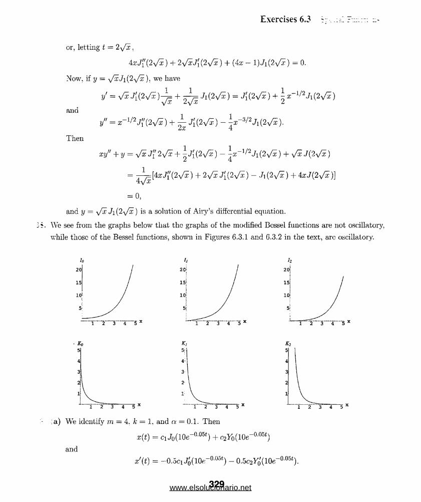
Exercises 6.3
or, letting t — 2-y/x.
4xJ'l(2y/x) + 2yfxJ[(2y/x ) + (4x - l)J i(2 V i) = 0.
Now, if y = y/xJi(2y/x), we have
and
Then
yr = 2v ^ )4 = + ttt j i(2vS ) = J i(2VS) + 5 i _ 1/aJ i(2vS )2\/x z
/ = x-I/2y;'(2V i) + ^ /;(2vS ) - ix - :,''2j1(2V5).
xy/f + y = V 5 J"2 V1 + 77 1(2\/r ] - i J;-|''2J 1(2v'x) + \/xJ(2y/x)2 4
= ^ [ 4 » J f ( 2 v ^ ) + 2v ^ J [(2Vx) - Ji(2Vx) +4xJ(2V®)]= 0,
and ?/ = J i (2\/x ) is a solution of Airy’s differential equation.
We see from the graphs below that the graphs of the modified Bessel functions are not oscillatory,
while those of the Bessel functions, shown in Figures 6.3.1 and 6.3.2 in the text, arc oscillatory.
h
Ko
;a) We identify rn — 4. k = 1, and nr. = 0.1. Then
x(t) = Ci Jo(10e_O'°D*) + C2io (10e_0'05t
and
*25
4
3
21
1 2 3 4 5
)
x'(t) = — O.ociJo(10e 00ot) — 0.5c2Vo(10e °-05*).
329www.elsolucionario.net

Exercises 6.3 Special Functions
Now ;x(0) — 1 and x'(0) = —1/2 imply
C1JO(10)+ C 2 )(l0) = l
c1^(10) + c2 o/(10) = l-
Using Cramer's rule we obtain
y0'( io )- r 0(io)
and
ci =
C-2 -
j 0(io)F0'(io) - ^ (io )y 0(io)
Jo(10) - Jo(10)Jo ( i0 )^ ( i0 )- ^ (i0 )y o( i0 ) ‘
Using Yq — —Yi and Jq - —J\ and Table 6.2 -we find c\ = —4.7860 and c2 = —3.1803. Tlr
x(t) = —4.7860,/q(10e_0105<) - 3.1803Fo(10e“005*).
40. (a) Identifying a = | , the general solution of x" + == 0 is
'1 /'l S/2x(t) = cix1/2.J1/3 ( j * 3/2J + C2X 1/2J _ 1/3
Solving the system x(0.1) - 1, x'(O.l) - — \ we find c\ — —0.809264 and c2 = 0.782397.
(b) *A
41. (a) Letting t = L — x, the boundary-value problem becomes
0'(O) = 0, 0(L) = 0,
where a2 = 5g/EI. This is Airy’s differential equation, so by Problem 35 its solution is
2 •} /o\ 1 /o _ / 2
d2d o „-pr + a tO = 0. at1
y -- Clt1/2J IJ3 Q o *372) + C2t1/2J- l/3 ( 3a i3 /2 ) = + 02^2W-
330www.elsolucionario.net
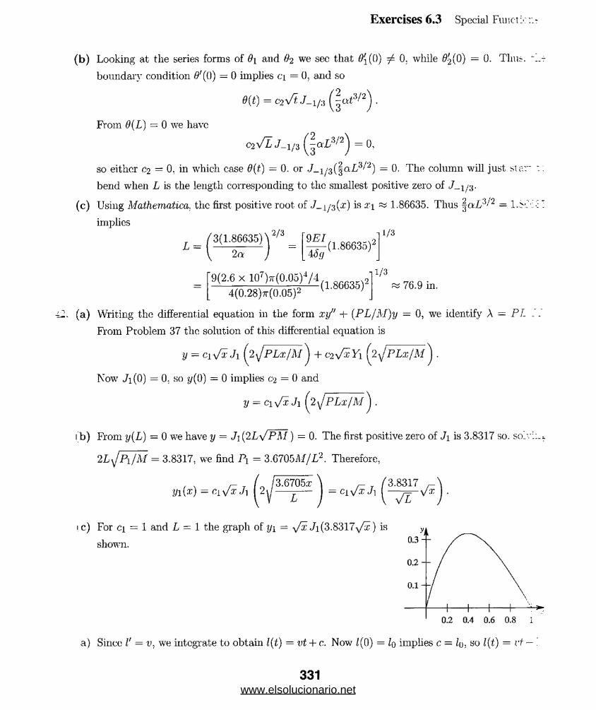
( b ) Looking at the series forms of 9\ and #2 we sec that #i(0) ^ 0. while 6 -2(0 ) — 0. Thus,
boundary condition #'(0) = 0 implies a = 0, and so
'2 ,3/2
Exercises 6.3 Special Functi':
6(t) = c2Vf. ./-1/3
From 6{L) = 0 we have
c2v/E,7_1/3 ( j a £ 3/2) = 0,
so either C2 = 0. in which case 0(t) = 0. or J ^ ^ ^ a L ^ 1'2) = 0. The column will just star
bend when L is the length corresponding to the smallest positive zero of J_ i/3-
(c) Using Mathematical the first positive root of J_ 1/3(0:) is x\ as 1.86635. Thus §a2/*/2 = l.SC
imphes
9EIL _ ^3(1.86635) y2/3
2a 4 fig(1.86635)2
1/3
9(2.6 x 10⁷)tt(0.05)4/4 r\2(1.86635)
1/376.9 in.
4(0.28)tt(0.05)2
(a) Writing the differential equation in the form xy" + (PL/M)y — 0, we identify A = PL
From Problem 37 the solution of this differential equation is
y = Ciy/x J\ ( 2 ^/PLx/M j + c^y/xYi ( l^P L x /M .
Now Ji(0) = 0. so y(0) = 0 implies 0 1 = 0 and
y = ci v/S Ji (2sJPLxjM ) .
ib) From y(L) — 0 we have y = J\ (2L y P M ) = 0. The first positive zero of J± is 3.8317 so. sol-
2Ly/Pi/M = 3.8317, we find Pi = 3.6705M/L2. Therefore.,
^ T . /3.6705# \ T /3.8317yi[x) = ci V# J a | 2y — - — 1 = c^ x J\ \ -—j= -\ /x j .
shown.
a) Since J/ = v, we integrate to obtain l(t) = vt + c. Now 1(0) = Iq implies c — so l(t) = vt
331www.elsolucionario.net
Exercises 6.3 Special Functions
Using sin $ & 9 in i d‘29/dt2 + 21' dOj dt + g sin 0 = 0 gives
, d20 n d.9 „ „(k + tJ0 ~ 2 ~dt~
(b) Dividing by v. the differential equation in part (a) becomes
^ ^ + 2 ^ + ^ = 0.v dt2 dt v
Letting x = (/q + vt)/v = t + Iq/v wc have dx/dt = 1, so
d # _ d B d x _ d £
dt dx dt dx
and(fO _ d{de/dt) _ d,(d9/dx) dx _ d2$
dx dt dx2 'dt2 dt Thus, the differential equation becomes
d2e n dB g „ nx-r^ - 2 - - + -e = 0
dx dx v
d2o 2 d9 g „ nor ~j~o --- 1— -- —dx* x dx vx
(c) The differential equation in part (b) has the form of (18) in the text with
1 — 2a = 2 =1
a = ~2
2 c- 2 = -1
b2c2 = 9-
a2 — p2c2 = 0
C 2
i=2vlp = 1.
Then, by (19) in the text
0(x) = x-W
or
m =V
\/ h) + vt
(d) Tb simplify calculations, let
qJi(2 v/!xI/2)+C2y,(2 v' 1/2)]+ I1*) j + rai'i i^\Jg(k+vt)
= 9 .! l ,1/2U= ~\/s(k) + Vt) =2yJ'-XX .
and at t = 0 let '«o ■ 2y/glo/v. The general solution for 9{t) can then be written
9 = C\u~1J\(u) + C2u-'Yl(u).
Before applying the initial conditions, note that
d9 __ dB du
dt du dt
332www.elsolucionario.net
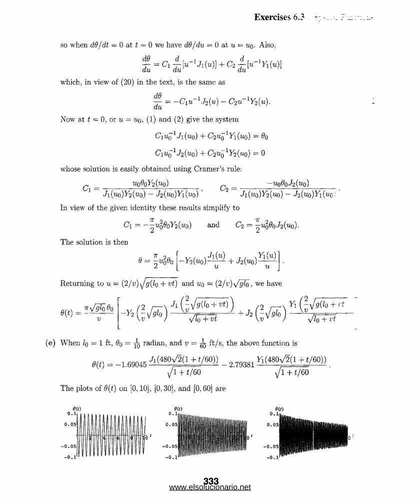
Exercises 6.3
£ = c I l i„-V l(«)] + c 2| ;i«- y lW i
which, in view of (20) in the text, is the same as
(10^ = -C'iW-1./2(«) - C2U~lY2{u).
Now at t = 0, or u = Mo, (1) and (2) give the system
Ci'Uq1 J i (uq) + C2'Uq1Yi (uo) = &o
Cyu.Q1 J2(«o) + C2Uq 1y2(uo) = 0
whose solution is easily obtained using Cramer’s rule:
uq9qY2(uq) n —uqi9o J2(yo)
so when dd/dt — 0 at t = 0 we have dd/du — 0 at u = uq. Also.
Ci = C2 —J i {tM))Y2(uo) - J2{uo)Y\(uo) " Jl(t<o)>2(wo) -
In view of the given identity these results simplify to
Ci = --UqBqY2 (uq) and C? = -'Uq(9qJ2('Uo).
The solution is then
, r , , Ji(tt) ,Yi(u) ->2(^0)-----^2(^0)u u
Returning to u = (2jv)^Jg(lo + vt) and uq = (2/v)y/gl(), we have
'2
,v
V
Ji (-^/gik + vt)
-*2 1; ) — j t = m — + v * J - V h + vt.
(e) When Iq = 1 ft., #0 = tTj radian, and v - tAj ft/s, the above function is
m = —1.69045 _ 2.79381 r i(«0 V 5 (l + */“ ))sJT+tJm
The plots of 0{t) 011 [0,10], [0,30], and [0,60] are
\J 1 4- i/0 0
m0.1
0 . 05!
-0 .05-0.1
333www.elsolucionario.net

Exercises 6.3 Spccial Functions
(f) The graphs indicate that d(t) decreases as I increases.
The graph of 6(t) 011 [0.300] is shown.
44. (a) From (26) in the text, wc have
Pq(x) = co
where
6-7 2 4 • 6 • 7 • 9 , 2 • 4 • 6 • 7 ■ 9 • 11 6 1-- tt- x H---- r.---$ = ------^----- x
2! ~ ' 4!
co = (-1)
6 !
3 l-3-5
2-4-6
0
16
Thus,
P6(x) = ( l - 21#2 + 6-3#4 - ^ - t^(231#6 - 315a:4 + 10-5#2 - 5). 16 V 5 / 1 6
Also, from (26) in the text we have
where
V(x) = ci ( x - -gp x +
ci = (-1)
6-9 3 4-6-9-11 5 2-4-6-9-11-13
5!
3 1 • 3 • 5 • 7
2-4-6
x —7!
x‘
35
16
Thus
P7(x) = (x - 9#3 + ^ X = -^(429#' — 693#° + 315#3 — 35#). 35 / 16
(b) Pq{x) satisfies ( l — ;?:2) y" — 2xy1 + 4‘2-y = 0 and P7{x) satisfies ( l — y" — 2xy' -4- 56y
45. The recurrence relation can be written
k
k = 1: P2 (X)
k = 2: P M
A-= 3: p40)
/,’ = 4:
9k 4- 1f t f . w - y n - x f t w - i + 1
2 5 o 3
Pfc_ i(z ); k = 2, 3. 4, ... .
_ 3 2 ^“ 2Ur' 2
_ 5r ( -X2
1
“ 3"r' \2 _ 2
_ 7 3
“ 43C K2X 2
_ 9 , f 35T-1 :“ 5'1l [ j X
/ o -j
3'X' = 2X 2‘
38) 5 v2"
3 \ 63 r 35 , 15
2X) = - T * + Y x
334www.elsolucionario.net

Exercises 6.3 Special Functions
* - * < * > = f **+f *h (f ** - f +1 ) - 231. 6 315 4x — — x + —r-.r“ — •
k = Q: Pi(x) = — X I ------— X~ ~r ~ rz rX6 /6313;c /231x6 _ 315^4 + 105^ _ _5_V r ( ^
7 V 16 16 16 16/ 7 V 8 ' 4 8
16 16
35 3 15
105 ,
16
429 7 693 * 315 ./ 35
= le "* “ I T ' + 16 ^ " 16*
46. If x = cos 6 then
dy . Qdy
d2y . 2 ad2y dy_ = sm » c J
and
sin + cos (9^ + n(n -f l)(sin#)y = sin# ( l - cos'2 9 ) ~ ^ - 2 cos 0^ + n(n + 1 )y = 0.
That is.
(1 ~ x2' ) U ' 2xt + n{n+1)v=0-
4". The only solutions bounded on [—1.1] are y = cPn(x), c a constant and n = 0, 1, 2 ,___ By
of the properties of the Legendre polynomials, ?/(0) = 0 or Pn(0) = 0 implies n must be odd. Thus
the first three positive eigenvalues correspond to n : 1, 3, and 5 or Ai = 1 • 2, A2 = 3 • 4 = 12, and
A3 = 5 • 6 = 30. We can take the eigenfunctions to be y\ = P\(x), y*z ~ Pz{x), and y% = P${x).
Using a CAS we find
1 d
2 dx
1 d2- t x~ — 1 r =
Pi(z
P2(x
P3(x
P a {x
Pk{x
P(i(x
(x2 - l ) 1 - X
222! dx2
1 d3
(.t2 - l)2 = i(3x2 - 1)
1
- 233! -fa* ^ “ 1)3 = 2 (5i:‘ ~ 3:C)
= ^ 2 ^ - V i = \ ^ - ' 30x'l + V
1 rP 1
= S i ? (X2 ~ 1)5 = 8 (6 3 l ‘ ~ 70x3 + I 5 l )
= 2 ^f (l2 - ^ = i b 31*6 - 31 fe l+ 10512 - 5>
1 cl~ < ~ 1 Pi{x) - ^ 7 (®2 ~ 1)' = ^(429x-' - 693x° + 315x>3 - 35x)
335
www.elsolucionario.net
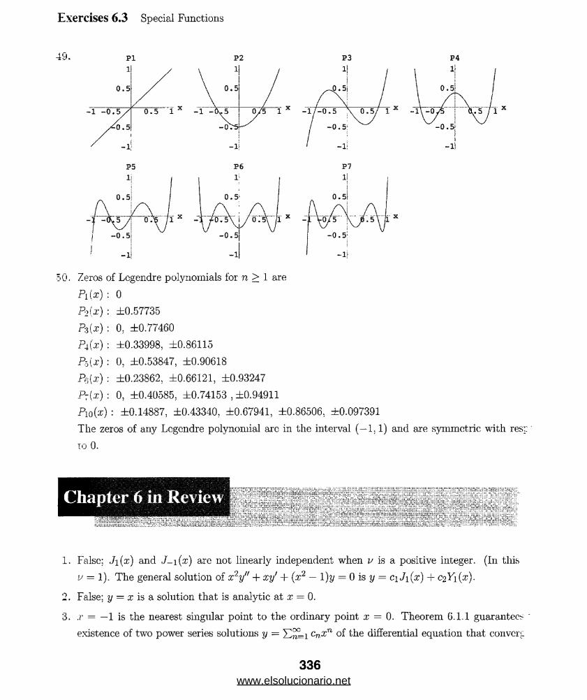
Exercises 6.3 Special Functions
49. p i P2 P3
P5 P6 P7
50. Zeros of Logendre polynomials for n > 1 are
P-2
h i
x)
x)
x)
0
±0.57735
0. ±0.77460
P4(x) : ±0.33998, ±0.86115
P${x) : 0, ±0.53847. ±0.90618
: ±0.23862, ±0.66121, ±0.93247
P-[x) : 0, ±0.40585; ±0.74153 , ±0.94911
P1Q(x) : ±0.14887, ±0.43340, ±0.67941, ±0.86506, ±0.097391
The zeros of any Legendre polynomial arc in the interval (—1.1) and are synunctric with res::
TO 0.
Chapter 6 in Review ; . ; ; ; ^ lv* * • 7;'f; ;; " 7 »' -c4 " ' - .....
" 7 / - - s . '5 \ V . ' . ' ......................' “ r •' - « ~ 5 < “ « - - - { - « ...................................,.......J ' ; r “ « s j.r.p ; ; ..c ;c --.'-W li' T ,w ,
1. False; J\(x) and J-i(:r) are not linearly independent when u is a positive integer. (In this
v = 1). The general solution of x2y" + xy' + (x2 — 1 )y = 0 is y = c\J\(x) + 0 }X\ (re).
2. False; y = x is a solution that is analytic at x = 0.
3. .r = — 1 is the nearest singular point to the ordinary point x = 0. Theorem 6.1.1 guarantees
existence of two power series solutions y — cnxn of the differential equation that convert
336www.elsolucionario.net
Chapter 6 in Review
least for — 1 < x < 1. Since —\ < x < \ is properly contained in —1 < x < 1, both power series
must converge for all points contained in — < x < | .
4. The easiest way to solve the system
2c2 + 2oi + Cq = 0
6cn + 4 C‘2 + ci = 0
12C4 + 6O3 - -Cl + C2 = 0o
20cs + 8C4 — -02 -T 03 = 0o
is to choose, in turn, cq 7 0, ci = 0 and cq = 0. ci ^ 0. Assuming that cq 7 0. c\ = 0, we have
C2 = - gOO
03
1
2*
23(
1
1
3*
1
= - 2 * 12°2 = “ 8C0
2 1 or, = - 7 C4 + 7J7-S2
o 30 20C3 = 60C01
whereas the assumption that cq = 0 . ci ^ 0 implies
o2 = -ci
2 1 1
3C2 6Cl -: 2Ci
1 1 1 5
2C3+
3GC1‘~ 12C2 ~ 36 C
2 1 1 1
5 ° 4+
30°2 '- 2q03 -
360ci.
five terms of two power series solutions are then
andyy(x) - cq
y2(x) = ci
1 -
1 3
" 3
1
~ 8X
A 1 1H-- x'
60
- ±r3 -0
36 ?2 360
The interval of convergence is centered a.t 4. Since the series converges at —2. it converges at least
mi the interval [—2.10). Since it diverges at 13, it converges at most on the interval [—5,13). Thus,
-t —7 it docs not converge, at 0 and 7 it does converge, and at 10 and 11 it might converge.
337www.elsolucionario.net

Chapter 6 in Review
6. We have
a:3 x 5
/ ( * • ) = — = X 6 , + 124°---------- - = X + Y + ^ +cosx „ x x* 3 151 — —“• -]-■ ■— — • ■ ■
2 24
7. The differential equation (x3 — x2)y" + y' + y = 0 has a regular singular point at x = 1 and ;
irregular singular point at x = 0.
8. The differential equation (x — l)(x + 3}y" + y = 0 has regular singular points at x — 1 and x = -
9. Substituting y = cnx"'+r i^to the differential equation wc obtain
OC
2xy" + yr + y = (2r2 - r) coxr_1 + Y \ 2(k + r)(k + r - 1 )ck + {k -f r)ck + c/c_i]xft+r_1 = 0k= 1
which implies
2r2 - r = r(2r - 1) = 0
and
(k + r)(2k + 2r - 1 )ck + ck_]_ = 0.
The indicial roots are r = 0 and r = 1/2. For r = 0 the recurrence relation is
c‘ = - fc (S ^T )■ * = 1' 2' 3.......
so
1 1 C l = - C O , C 2 = - C O , C 3 = - g p C 0 .
For r = 1/2 the recurrence relation is
v k = w .......
SO
Cl = - 500, c2 = ic „ , c3 = - ic o .
Two linearly independent solutions are
and
V2= i .V2 f 1 _ 1 + 1 2 _ 1 3 + . . . V
V 3 30 630 )
338www.elsolucionario.net

Chapter 6 in Review
.0. Substituting y = cnxn into the differential equation we
OO OO X,n~ 'nr„. Tn — V r-../ -xyf -y=Yl n (n ~ x)°n^ ~ YI nc xtl
n=2 n=lk=n- 2
oc oc
= Y ( k + 2)(A- + l)Ck^-2'J'k - Y kckXk - S ckXk k=0 fc=l fc=0
oc
= 2c2 - Co + ]£[(& + 2)(fc + l)cjfe+2 - (k + l)cfc]«fr = 0. k=i
2 C<2 — Co = 0
(k + 2)(k + l)cfz+2 ~ (k + l)cjb = 0
C2 = ^
1Cfc+2 = ^ X 9 Cfci Ar = 1,2,3,... .
Thus
and
Choosing cq = 1 and C] = 0 we find
1
C2 = 2
C3 = C5 = cr = ■ ■ ■ = 0
1
*‘ = 8
a s = iand so on. For co = 0 and c\ = 1 we obtain
C2 = C4 = c% = ■ ■ ■ = 0
1
j
1
5
°7 = 105
C 5 = 15
and so on. Thus, two solutions are
1 9 1 4 1 g
w = 1 + 2r ' + r + 4?c + - -and
339www.elsolucionario.net

Chapter 6 in Review
1 3 1 5 1 7* - * + ? + « * + M5* + " "
11. Substituting y = c‘nXn into the differential equation we obtainoc
(x — 1 )y" + 3y — (—2c2 + 3co) + 53 [( + — (k + 2)(k + l)c^+2 + ^ck[x. — 0fe=i
which implies c2 = 3co/2 and
(k + !)kck+i + 3 Ck
C*+2 = (* + 2){fe + 1) ' k = 1' 2’3-'--
Choosing cq = 1 and cj. = 0 we find
3 1 5
2'
and so on. For cq = 0 and c\ = 1 w e obtain
C2 = 2' °S = 2' C4
C2 — 0, C‘3 = C'4 — ~1
2* 4and so on. Thus, two solutions are
» “ i+ 2* + r + ? + ' "and
i 3 i 4 i 1/2 = X + - X + j X H--- .
12. Substituting y = Y,^Lq cnxn into the differential equation wo obtainOC
y" — x?y' + xy = 2(>2 + (603 + co)x 53 [( + 3)(fc + 2)c^+3 — (/c — l)cfcj3:,‘’+i = 0k=1
which implies c-i = 0, C3 = — c q / 6 , and
k — 1
° ^ 3 = (fc + 3)(fc + 2)C*' 2> 3> • * • •
Choosing co = 1 and ci = 0 we find
1
C3 _ 6
(■4 = C7 = 6*10 = • • • = 0
CJ5 = c 8 = = • • • = ()
c6 = _ 90and so on. For co = 0 and c\ = 1 wc obtain
C3 = Cg = CA) = ■ ■ • = 0
C4 = C7 = C1 0 = ■ • * = 0
05 = Q3 = Cl 1 = • • • = 0
340www.elsolucionario.net
Chapter 6 in Review
yi = 1 - \xz - -J-x6 --- and y2 = x.6 90
3. Substituting y = CnXn+r into the differential equation, we obtain
OCxy" - (x + 2)y' + 2y = (r 2 - 3r)eoxr _ 1 + Y [(fc + r)(fc + r ~ %)ck
k—l
— (k + r — 3)cA,_i]xfc'Hr_1 = 0:
which implies
r2 - 3r = r(r - 3) = 0
and
(k + r)(k + r - 3)cfc — (fc + r — 3)c^_i = 0.
The indicial roots arc n = 3 and r-i = 0. For r2 = 0 the recurrence relation is
k(k - 3)ck - (k - 3)cfc_1 =0 , k = 1, 2, 3, ... .
Thenci - c0 = 0
2c2 - ci = 0
0c;j — 0c2 = 0 =^- c‘3 is arbitrary
and
Cfc = -Cfc_i, fc = 4, 5, 6 , . . . .
Taking co 7 0 and C3 = 0 we obtain
ci = Cq
and so on. Thus: two solutions are
1
2‘
c3 = C.4 = C5 = • • • = 0 .
Taking cq = 0 and C3 ^ 0 we obtain
www.elsolucionario.net
Chapter 6 in Review
and so on. In this case wc obtain the two solutions
1 9yi = 1 + x + -xr
and
2/2 = X 6 + ^ x ° + ^-X -6 H-------= 6ex - 6 ^ 1 + z + .4! 5! 6! V 2 /
14. Substituting y = cn^n into the differential equation we have
(cos x)y" + y - ^1 - ^x2 + ~ x j - H-- j (2c2 + 6C3X + 12c4::r2 + 20c$x3 + 30c6;r4 +
+ £ c„z"n=0
= 2r>2 + 603;!' + (12C4 - C2)x2 + (20c5 - 3c3)x3 + ^30q; - 6c,t + a;4 H--
+ [co + cja: + C2.T2 + 03a;3 + C4.T4 H-- j
= (co + 2c2) + (ci -r 60-3)0: + 12c4;r2 4- (20c,5 - 2cs)x'i + ^30c(j - 5c4 + ^ c 2 j x4 H--
= 0.
Thus
and
co + 2C2 = 0
ci + 6c;? = 0
12c4 = 0
2 0 c5 - 2 c3 = 0
30c6 - 5c/| + - C2 = 0
C 2 = ~ 2 C 0
C 3 = - 7 C 16
C4 = 0
C o - 10C 3
ce 604 36002 ‘
Choosing cq = 1 and cj = 0 we find
c2 = — x , C3 = 0, C4 = 0, C5 = 0. cq —2 ' ’ ” 7 " ' u 720
342www.elsolucionario.net
Chapter <? in Review
and so 011. For cq = 0 and c\ — 1 we find
C2 0, C3 , ( * 4 0* •
0 ’jL
and so on. Thus, two solutions are
Lo.
Thus
and
1 1 2 1 6 , 1 3 1 -Vi = 1 — - I + ——:i H-- and y2 = x — -x — —x" — • • ■.2 720 6 60
y" + xy' + 2y = 53 n(n “ l)e»£n-2 + 53 ncn^n + 2 53 cH-r"w=2 __________ n = l n=U ^
k ~ n - 2 k = n k = n
oc oo oc
= 5 3 (fe + 2)(fc + i)Q :+2'i'fc + 53 + 2 5 3 fc=0 &.=1 fc=0
0 0
= 2c2 + 2cq + 53 [( + 2)(A: + l)cfc+2 + (& + 2)cj;ja/ = 0. k=1
2c2 + 2eo = 0
(fc + 2)(A: + l)cfc4-2 + (k -j- 2)c^ = 0
C2 “ —Co
Cfc+2 - Ck- k = 1,2,3,... .
Choosing co = 1 and C\ = 0 wc find
c-2 = -1
c3 = c5 = c7 = • ■ • = 0
Ci = 3
1
C6 = ” 15and so on. For cq = 0 and ci = 1 we obtain
C2 = C4 = eg = • • • = 0
C3 = -2
1
1
Cs 8C? 48
343www.elsolucionario.net
Chapter 6 in Review
and so on. Thus, the general solution is
1 , 1 « . \ „ f 1 , 1 , 1„ = f t ( l - *» + j** - + ■••)+ C, ( , - j * 3 + ^ + .. .)
y' = a , (-2,, + |tf> - I * 5 + . . . ) + C ,( l- § * * + |*4- 5 * * + - ) .
Setting y(0) = 3 and y'(0) = —2 we find co = 3 and ci = —2. Therefore, the solution
initial-value problem is
y = 3 - 2s - 3x2 + x3 + x4 - - \x* -t- ± -x7 + ■■■.4 o 24
16. Substituting y = cn£n into the differential equation we have
OCn
(x + 2)y" + 3j/ = 53 n(n - 1 )cnxU 1 + 2 £ n (n — ty'nX" 2 + 3 53 cn®’7 1 = 2 7 1 = 2 T i= 0
Thus
and
k—n —l k—n —2 k = n
OG OC OC53 (k + l)^ cfc+ia-/" + 2 53(fc + 2) (A’ + l.)cfc+2;t'fc + 3 53
— 4c.‘2 + 3co + 53 [(k + l)fecfc4-i + 2(fc + 2)(A: + 1 )c&+2 + 3c*;]:cfc — 0. fc=l
4c2 + 3co = 0
(fc + l)fccfej_i + 2(A; + 2)(fc + l)c/--j_2 + 3c/,; : 0
3C2 : --C0
Ch+2 = ~ 2(A + 2) Cfc+1 “ 2(A: + 2) (A + 1) Ck> * = 1'2’3’Choosing Co = 1 and ci = 0 we find
3
www.elsolucionario.net
Chapter 6 in Review
and so on. For Co = 0 and c\ = 1 we obtain
C2 = 0
1
1
Lf
c5 = 0
Ci = 7F 16
and so on. Thus, the general solution is
1 , 1 , 9y = C0 { l-- ,x ‘ + ^ + ~ x ' - ^ + ---)+Cl ( x - - x ^ - x i +
and
y/ = C o (- ^ + 5 x 2 + i :c9 - ^ ‘' + .. . )+ C I ( l - ^ + i a:3 + . . . ) .
Setting y(0) = 0 and ?/(0) = 1 we find cq = 0 and a = 1. Therefore, the solution of the initial-value
problem is1 ‘3 1 4
y = x ~ i x i$x -■■■■
The singular point of (1 — 2 sin x)y" + xy = 0 closest to x — 0 is tt/6. Hence a lower bound is 7r/6.
'.S. While we can find two solutions of the form
Vi = co[l + ■ • • ] and i/2 — c\[x H-- ],
the initial conditions at x — 1 give solutions for co and c\ in terms of infinite series. Letting t = x — 1
the initial-value problem becomes
lit? + ^ + ^ eft + V = ° : = _6, y/^ = 3'
Substituting y = °ntn into the differential equation, we have
j 2 ?/ j } o c o o o c o cj + (£+1) — + ?/ = 53 n (n ~ l)cntn 2 + 53 ncntU + 53 ncnta 1 + 53
n—2 n= 1 n=l ;?~0
k = n —2 k—n k—n- -1 k = n
oc oc oc- oc-
= 53 (^ + 2)(fc+ i)ck+2 tk + 53 kcktk + 53 + ^)ck+itk + 53 k= 0 fc= 1 k=0 fc= 0
oc-= 2 c2 + Ci + co -+- 5 3 [(^ + 2 )(fc + l ) c ^+2 + ( k + l ) c ^ + i + ( k + l)c jt ] t^ = 0 .
k= 1
Thus 2c2 + ci + co = 0
(k + 2)(k + l)c^+2 + {k + l)cfc+i + (& 4- l)c& = 0
345www.elsolucionario.net

Chapter 6 in Review
and c 2 = --ci + CQ
2
Ck-2 -- - C~tLV - , k = 1,2,3.......k + 2Choosing cq = 1 and c\ = 0 we find
c2 — ~ x • C‘i = ~ . C4 = — 2 6 12
and so on. For co = 0 and cj = 1 we find
C2 = , ca = -
and so on. Thus, the general solution is
V = c01 1 , 1
6 ’
ci
C4 = 7 ,
1 1 1
6 62’ ' 6' ' 12
The initial conditions then imply co = —6 and ci = 3. Thus the solution of the initial-value prc'
is
y = -6 1 - - l)2 + - l)3 + ^(.x - l)4 +
+ 3
19. Writing the differential equation in the form
and noting that
„ / l — c o s . t \ .
y + ( — -— h/ + xy 0,
1 — COS X X Xs X 5
x = 2 ~ 24 + 720
is analytic at x = 0, we conclude that x = 0 is an ordinary point, of the differential equation.
20. Writing the differential equation in the form
xv" +
ex - 1 - xy = 0
and noting that
a-2x 2 2 x
ex — 1 — x ~ x ~ 3 + 18 + 270
we see that x = 0 is a singular point of the differential equation. Since
•2 f xx.x3 x42x2 _
— O <7> 1 Ie* - 1 - x j ~ ~ ~Y 18 "r 270
we conclude that x = 0 is a regular singular point.
346www.elsolucionario.net

Chapter 6 in Review
1. Substituting y = °nxn into the differential equation we
OO OC OCy" + x2y' + 2xy = £ n(n - l)c„a;n_2 + 53 + 2 53 cn-
?7~2 n= 1 n=0
k—n—2 k=n+l k=n+1
OC o o o c
= + 2)(k + !)cfc+2 ^ + £ (k - l)cfc_jx* + 2 5 3 c*-i-rA’ fc—0 Ar=2 fc=l
OC= 2c-2 + (6C3 + 2co):e + 53 i(k + 2)(fc -t- l)Cfc_-2 + (k + l)c/j_i]:i. = 5 — 2.:' —
k = 2
Thus, equating coefficients of like powers of x gives
2C2 = 5
6C3 + 2co = — 2
12c’4 + 3ci = 0
20cs + 4c2 = 10
(A' + 2)(k + l)c%+2 + (k + l)cfc_i = 0, k — 4 .5 ,6 ,...,
and
C2 = 2
63 = ~3C0 " 3
. _ 1 1 . _ 1 1 f 5\ _nC° 2 5°2 2 5 V2 j
1
" ~k
Using the recurrence relation, we find
Cft+2 k + 2 Ck~1'
www.elsolucionario.net

Chapter 6 in Review
CJ.2 = -T7Tc9 = CQ +12 34 • 4! 34 • 4!
1 1C13 = ~ T ^C0
13 v 4 • 7 • 10 • 13Cl
and so on. Thus
V = co1 3 1 g I n 1 19
1 ~ 7;% + T o — r ; « — t , — TTiC + — -------77 X —
+ C1
3’' 32 -2f' 33 • 3!' 34 • 4!"
1-x10
11 4 1 7
x ~ l x + 4^7X ~ 4 • 7 • 10" ‘ 4 -7-10 -13x 13 -
+ 5 2 1 3 1 6— 7 — —7 ----J — -2 3 32 • 2! 33 • 3! 34 -4!
*9 + *12-
, . _ 1 du ,22. (a) From y ------— we obtain
u dx
dy 1 d?u 1 / dll'
dx u dx2 u2 \ dx ,
Then dy/d.x = .t2 + y2 becomes
1 d2u 1 ( dux 22
1 — 2 I { du \
u dx2 w2 i cfo j X u2 1 dx J
d2u 2 so + x u = 0.
(b) The differential equation u" + x2u = 0 has the form of (18) in Section 6.3 in the text wit:
1 - 2a = 0 a =
2c —2 = 2 c = 2
1b2c2 = 1 b =
P = Aa 2 — p 2c2 = 0 =
Then, by (19) of Section 6.3 in the text,
J/2 C 1 J 1/4 Q z 2 ) + C 2J _ i /4 Q x 2 ) .U = X
348www.elsolucionario.net
Chapter 6 in Review
(c) We have
1 du du dx xl/'2w(t) dx
x1/2w(t)
1
xWw
1
xll'\v
1
2xw
" dt <lr, 2"
3/2 a wdw+
dt 2.x1/2
o eiti!2ar— + w
dt 2xiu
, , dwAt —— |- w
dt
Now
At — + -ir — — (ci J-i/4(t) + c2J_ i/4(i)] + c\Ji/4{t) +dt
= U1
so
C1 ^-3/4 (*) _ 4t'^1/4^ ) 0 1 ( “ 4 - V 4^) — 3/M
+ C lJ l/S ) + °2J-l/^{t)
= 4cit J_3/4(«) - 4c2f J3/4(£)
= 2cin’2 J_3/4 Q;j;2) - 2c2x2Jy 4 Q.x2) ,
2cix2 J_3/4(^r2) ~ 2c2:r2J3/4(lx 2)y =
2x[ci J 1/4(ix 2) + c2J_ 1/4( i« 2)]
—ci J-3/4( ^ 2) + c2J3/4(^ e2)
Cl J i/4( ^ 2) + c2 J _ i/4(|j;2)
Letting c = c,\fc2 we have
_Jm ( ^ ) - c J _ m (±x2)
cJx/A{\x2) + J_1/4(^C2)
a) Equations (10) and (24) of Section 6.3 in the text- imply
cos f J 1/2{x) - J _ 1/2{x) i 21 /2 (*x‘) = - y — COSX
349www.elsolucionario.net
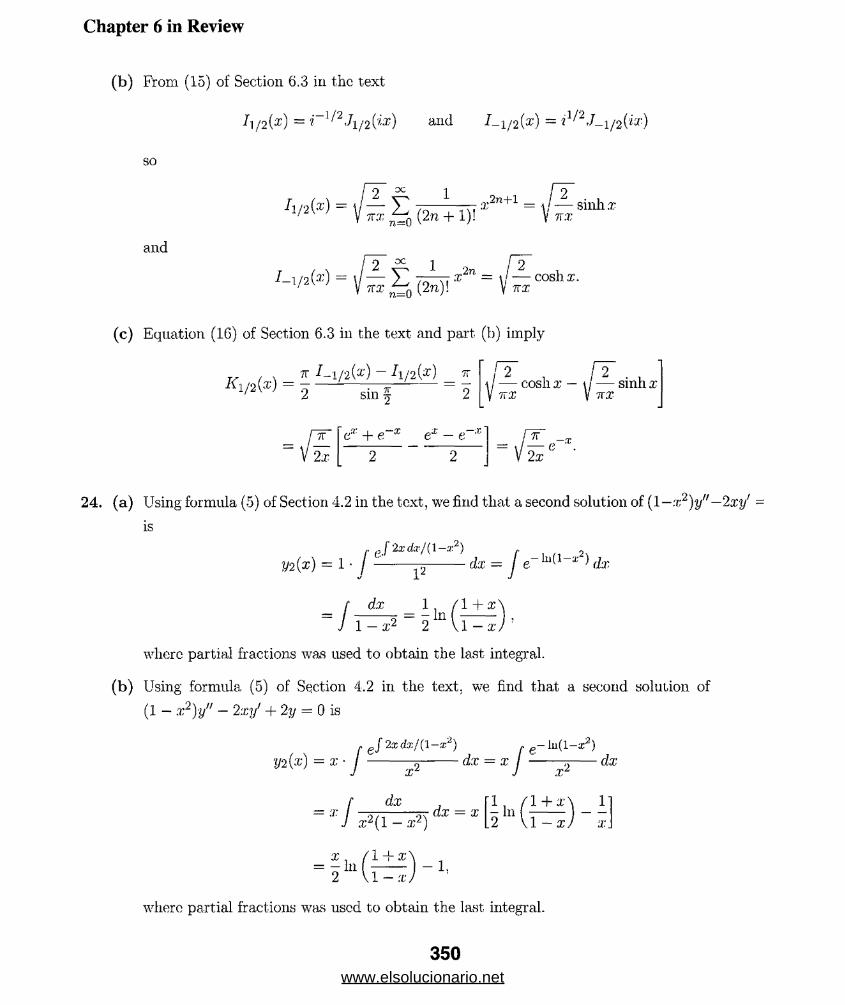
Chapter 6 in Review
( b ) From (15) of Section 6.3 in the text
I , /2(x) = r ' / 2J1/2(ix) and I . i n (x) = !1/2./_1/2(!x)
SO
and
11 /-){x) — W— 53 7 ——777 2,1+1 = — sinli.rV z- (2n + 1)! V nx
/_! /2(-J’) = \/— 53 7o\i :c2” — \ l~coshx. V7ra’ ^ 0 (2n)! V ^
(c) Equation (16) of Section 6.3 in the text and part (b) imply
~ , N tt /-1/2W - A/2(*) A i/2(® )= 2 — — ----sin
1 / — cosh x — \j — sinh xV nx V 71
ea: + e“x e* - e"*
2
24. (a) Using formula (5) of Section 4.2 in the text, we find that a second solution of (1—x2)y'
is
er ( J ' ^ d x / n - x 2)3/2(x) = 1 • j ---- p ---- dx - j e~h - 'x > rfa:
f dx
J 1 — x2
dx 1, f l+ x In
2 VI - x ) ‘
where partial fractions was used to obtain the last integral.
(b) Using formula (5) of Section 4.2 in the text, we find that a second solution o
(1 — x2)y" — 2xy' + 2y = 0 is
. ef 2x d x / ( l- x 2) . e- ln ( l—in2)mix) = x - j ----^ ----dx = x J ---^ -- dx
= x f dx = x \lh i( l ± £ ) . lJ x2(l — x2) L2 \l~xJ x
= £ ln f I ± £ W2 VI - x
where partial fractions was used to obtain the last integral.
-2 xy1 =
350www.elsolucionario.net

Chapter 6 in Review
25. (a) By the binomial theorem we have
,—1/21+ (t2 — 2xt^ 1 = 1 — ^ (t2 — 2xtj +
( 1/2) ( 3/2)
2!(t2 — 2 xty
+ ( -1/ 2K-3/2X-5/2) (t2 _ ^ 3 +ui
= 1 - - 2a’*) + f (*2 - 2-^)2 - 77^2 - 2a;i)3 +16'
1 1= 1 + xt + ^(3a^ — l)t2 + ^(5«t3 — 3:r)i3 H--
= Z Pn(^)in■n = 0
(b) Letting x = 1 in (1 — 2xt + t2)_1//2, we have
(1-21 +12)~1/2 = (1 - 1r 1 = —^ = 1 + < -f i2 + i3 + ... (|*| < 1)X “ t/
oc-= £ «"•n=0
From part (a) we have
Pn(l)tn = (1 -2 t + t2Y 1/2 = £ tn.n =0 n = 0
Equating the coefficients of corresponding terms in the two series, we see that -PM(1)
Similarly, letting x = — 1 we have
(1 + 2< + 12)~1!2 = (1 + 1)"1 = 7——7 = 1 — t+ t2 — 3t3 + . . . (|t|<l)1 —r~ t
•DC OC
n=0 7i=0
so that Pn(—1) = (—1)".
351www.elsolucionario.net

7 The Laplace Transform
1. y {/(()} = faDC 1
(-stdt = -e s
2
1 1— - e -s t
o s 1
= -e"" - - - (o - -e"*) = -e“* - - . s > 06‘ S \ S J S S '
2. i ? { /'(£)} = [ te~*ldb = --&-* = — (e-2 * - 1), s > 0Jo 6- o s
3. l£{f{t)} = j^te~ stdt +
1 _ e 1
30 e d t = (--te-* - \e~st s
1
1 1 DC- V *
o s
= [-~e~s - ^e~ s ) - f 0 - 4 ) - -(0 - e~8) = ~(1 - e~% s > 0s2 j s
4. X{f(t)} = £ (2 t + l)e-stdt — te s
— s t st 1 -st
2 _ s 2 _a 1 — e -- 7 > e -- e •Q C - O
2
5 6‘
2 1\ 1
2 = -(1 - 3e lS) + (1 - e 5), 6* > 0
5. = I (shlt)e s t ' d t = 8i*in t~ ' ^ P i t-e st cos t
= (0 + ^ - e - ^ - A ) 1■s2 + 1
cub i i e '/2'
1
6'2 + U ,S‘2 + 1(e_7rs + 1), s > 0
6. J£{f(t)}= I / (cost)e std t— ( — 2S e ,stcos/; +Jir/2 \ 5 + 1 ! 2 t 1
e st sm tt t / 2
= 0 - 0 4•S + 1 *2 + r
tts/2 s > 0
7. /(t) =0, 0 < t < 1
t t > 1
—.sf 00 1 1 = — € ~\~ “rr 6 S > 0
1 S S Z
8- fit) =0 < t < l
2t-2. t > 1
352
www.elsolucionario.net
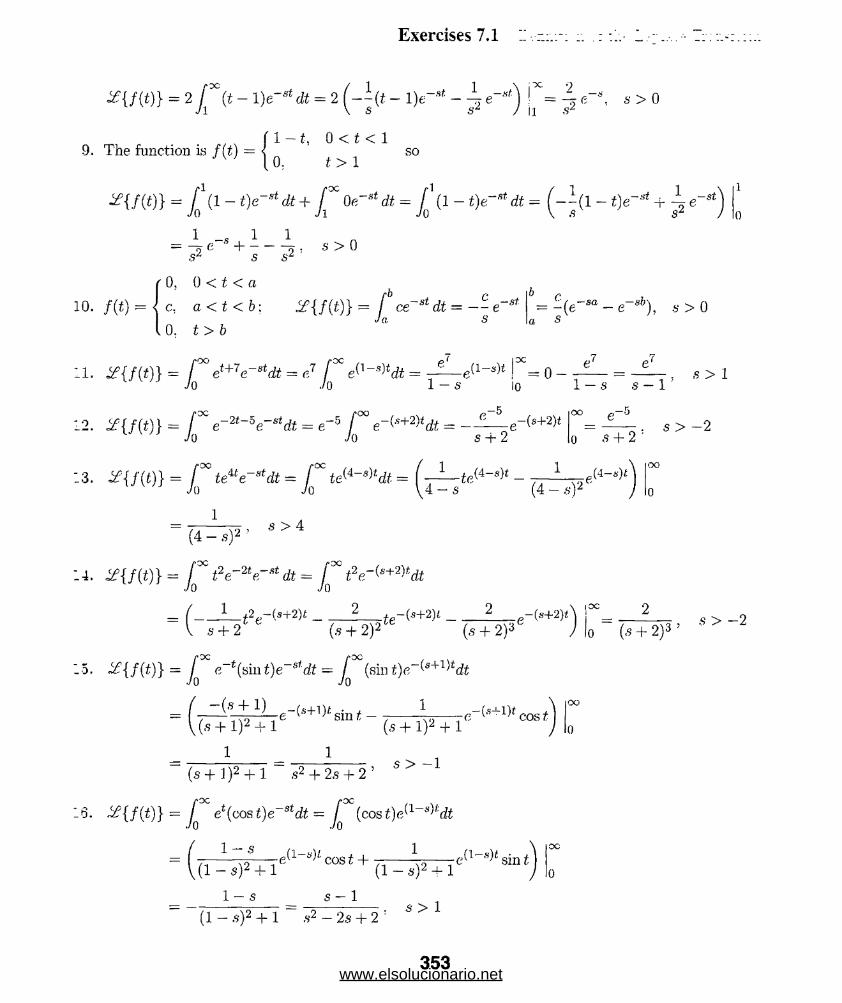
Exercises 7.1
^{/W} = 2 {X(t-l)e-«dt = 2 f = 1J 1 \ S Sz J I I A
, , r i - t, o < t < i9. The function is f (t) = < so
Jy ; 10. t > 1
= f (1 — t)e dt+ I Oe st dt = I (1 — t)e 8t dt = ( —-(1 — t)e st + 4J 0 J 1 J 0 \ <9 S*
io. m =
= \c-* + - - \ . s > 0s s sz
0, 0 < t < a
c, a < t < b ; {/(£)} = [ ceJa
, 0. t > b
—st dt = — - e s
= ~(e~sa - e-**), aa 5
/•OC /’OO12.2 { f ( t ) } = J e-2t~5e-*tdt = e-5 j e~^+2 dt =
1GII11-----------------------------------------1e7
10 1 — s s
.,—5. r-(«+2)t
o° g -5
s + 2 0 3 + 2
■fet4-)* , 1(4 — *O2 J
s ?
, s > 4(4 — s)2
14. # { / ( * ) } = r t2e-2te~8td t= r f e r ^ ^ ' d tv o 0
= f---£2e~(s+2)tV s + *2 2 te_ (s+2)i _____-___^-(«+2)A 1°°— 2
-0.
(,9 + 2)2^ (s + 2)3
#{/(*)} = f 00 e~t(smt)e~stdt — f°° (s in ^e ^+ ^d t•j 0 */ 0
o (.9 + 2)3 ’
= ( ' ^ s + iL e-(«+iKs in (_\(s + l)2 + l
1 1
(s + l)2 + 1
, s > — 1
e 0s • l)* cos f
(s + 1)2 + 1 s2 + 2,s + 2
16. ^ { /( i)} = I* et (cos t)e~st dt = f (cos i j e ^ ^ ’dt
1 — s
(1 — s)2 + 1
1 — S
s(l r-nscosi +
S — 1
( l- s )2 + le ( 1 »)t g j n i
oc
(1 - A-)2 + 1 A-2 -25 + 2. s > 1
> 0
s > 1
- - 2
s >
353www.elsolucionario.net
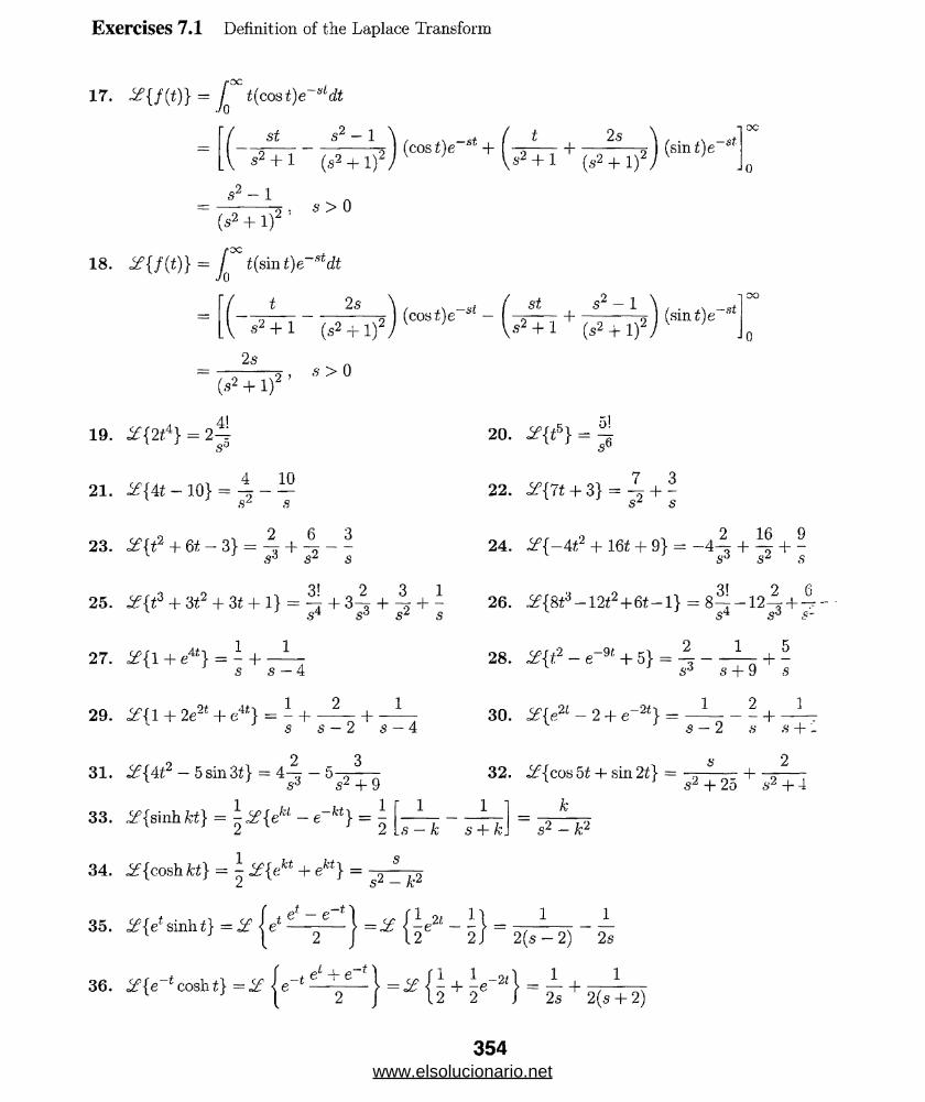
Exercises 7.1 Definition of the Laplace Transform
17. if{ /(t)} = j t(cost)e s'
st
~sldt
s2- 1
+ 1 (s2 + 1)"(cost)e- + ( ^ 4- (sint)e-sf
OC
s2- ls > 0
2 s
s2 + 1 (s2 + 1)2 . (cost)e - ( 3 ^ 7 + 717— ^ 2) (sini)e
y + i (s-2+ ir ,
OO
2s
(*2 + 1) ’
.4!
.9 > 0
19. if{2t4} = 2 j
4 1021. i f {4t - 10} = ^ - —
23. i f {t2 + 6 i-3} = -^ + - ^- -5 s
3 13[ 2_ _
s4 s3 s2 + s
27. if { l + eAt} = - +1
29. if{ l + 2e2i + e4t} = - + ——7: +
s s — 4
1 2
31. if{4£2 — 5 sin 31\ = 4^- — 5-=— - 1 J s3 s2 + 9
33. if{sinhfci} = ^ if{ e fct — e~kt} = ^Zt £
20. ^ = $
22. ¥{7t + 3} = + -
24. if{ —4tf2 + im + 9} = -, 2 It
_4? + ?
26. i f {8t3 —12£2+6f—1} = OO
*11
£2
1 to 1
28. if{ i2 - e"* + 5} = |1
5 + 9 "*
30. X{e21 2 + e~2t} =s
1 2
-2
32. i'-Jcos 51 + sin 2t} =8
+ 25 ' A’
s — k s + k. s2 — k‘2
34. i f {cosh kt} = 1 2{eu + eH} =s2 - k2
35. if{e‘ sinhi} = y |e* - i } = - ±
36. ^ - ‘ oosh t) = 2 |e-‘ = X {5 + je " 2'} = ^ + ~
1 9r H—
,s
2 6
J* 5'
5
s
1
A1 + -
2
^+4
354www.elsolucionario.net

Exercises ".1 I - : . . . .
7. {sin 21 cos 2t} = j sin 4i j = g2~ Tfg
5. ^f{cos2t } = if |^ + ^cos2i| = ^ + ^ 6s2 + 4
9. From the addition formula for the sine function, sin(4i + 5) = (sin 4i)(cos o i — cu? 4~
^{sin(4t + 5)} = (cos 5) i f {sin At) + (sin 5) i f {cos 4/}
4 s= (cos5) V , ~-,r + (s in5 ) 9 7 Tr + 16 sl + 16
4 cos 5 -f (sin 5) s
= s2 +16 ‘
0. From the addition formula for the cosine function,
( tt\ tt . . 7T \/3 1 .cos £ — - J = cos t cos - + sin t sm — = cos t -i- - sin t
\ 6 / 6 6 2 2
so
!£ | cos (t - ^ | = — % {cos t} + ^ {sin t}
_ y/Z s 1 1 _ 1 ^ S + 1
“ T s2 + l + 2 s2 + l ~ 2 ~ ! ? ^ T '
1. (a) Using integration by parts for a > 0.
T(a + 1) = j tae~t dt = —tae~i j + a j dt = ar(ai).
(b) Let u = st so that du = s dt. Then
***“> = r e~"ed t ~ r e_“ i *■= ? ^ r (a + j) ’ a > ~L
, w
(b) X{tm } = ^ ^
(c) ^ ^
i. Let F(t) = tl-! i . Then F(t) is of exponential order, but f(t) = F'(t) = gi_2/3 is unborn
t = 0 and hence is not o.f exponential order. Let
f(t) = 2tet cost/ = ~ sinef2.JK dt
355www.elsolucionario.net
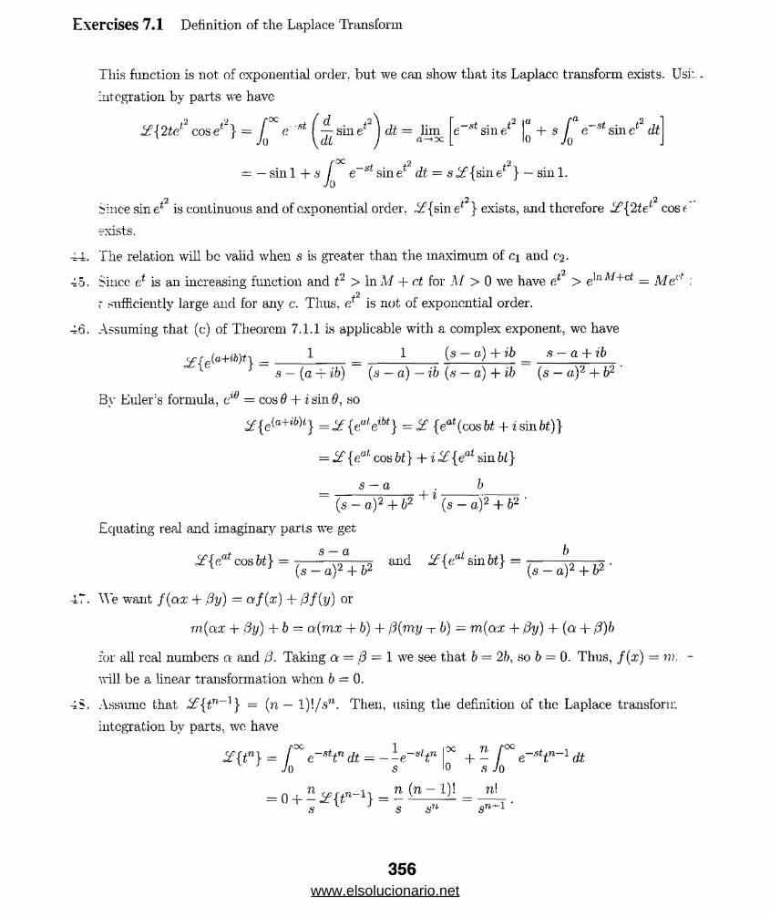
Exercises 7.1 Definition of the Laplace Transform
This function is not of exponential order, but we can show that its Laplace transform exists. Usi:..
integration by parts we have
i£{2t,el2 cose4"} = [ e st ( -7 - sine* ) dt = lim e~'stsine£ + s ( e~stsinef dt1 1 Jo \dt J [ 0 Jo
= — sin 1 + s j e~st sin e* dt — s^£ {sin e* } — sin 1.
Since sine* is continuous and of exponential order. {sine* } exists, and therefore !£■{2tel cose
exists.
44. The relation will be valid when s is greater than the maximum of c\ and o>.
45. Since et is an increasing function and t2 > In M + at for M > 0 we have ef > eln M+ct = Mect :2
r sufficiently large and for any c. Thus, e* is not of exponential order.
46. Assuming that (c) of Theorem 7.1.1 is applicable with a complex exponent, we have
v/>+«>)n = 1 = 1 (* ~ °) + ib =s — (a 4- ib) (s — a) — ib (s — a) 4- ib (s — a)2 + b2
By Euler’s formula, c1'0 = cos 0 + i sin Q, so
y { c(a-N6)i} = ^ { e«V w} = «Sf {eat(cos bt + ism bt)}
= {eai cos bt} + iX {eat sin bl}
s — a . b+ i
(s — a,)2 + b2 (s — a)2 + b2 '
Equating real and imaginary parts we get
¥{eat cos bt} = -— - v>a—-k and &{ealsmbt} = ^ — p? .(s — a)2 + bz (.9 — a)z + \r
47. We want f(ax + dy) — atf(x) 4- ,8f(y) or
m(ax 4- By) 4- b — a(rnx 4- b) 4- ff(my -- b) — m(ax + j3y) + (a + d)b
for all real numbers a and 0. Taking a = l3 — 1 we see that b = 2b, so b = 0. Thus, f(x) = m..
will be a linear transformation when 6 = 0.
45. Assume that ^£{in~]} — (n — l)\/sn. Then, using the definition of the Laplace transform
integration by parts, wc have
&{tn} =
= 0 + - <f un's
-L oc n /,cc-e t _ + - /s
0
n ( n — 1)! n!
s sn sn~i •
356www.elsolucionario.net

Exercises 7.2 Inverse Transforms and 1;
,s3J 2 Is 3/ 2
o ^f-i/J_\ — — I^3« « C s 6 ' 1 1 1 “ - A i / — _ 1/U4 J 6 I *4 I 6
« . „ - . { ! ^ 2 } . | } . . * . * » ■
S. + ---- }= if~ 1 (4-i + I . ^ - - i - l = 4 + ^ 4-e-8tIs s° s + 8 J [ s 4 5° .9 + 8 J 4
9 - ^ {sriK M rT iT iH ^ 410- ^ ‘ { ^ - ^ “ { s - r i T s } - ^
n - ■sf" 1{ ? T « } = i f “ , { ? - ? T 4 9 } = ? sin7t
12. -| = 10cos4<I s2 + 16 J
:3- ^ " 1{ 4? ? l } = ^ 1 { ? T w } =cos5t
:4- ^ ' ' { 5 5 T l } = ^ " 1 { 5 '? T 1 7 l} = 5 si4 *
ives
357www.elsolucionario.net
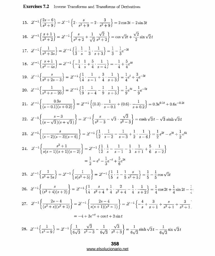
Exercises 7.2 Inverse Transforms and Transforms of Derivatives
15. if '
16. se
t t . i f
IS. if '
19. i f
20. if '
21. if '
2 2 . i f '
23. if "
24. i f
25. Jf-
26. i f '
27. ^
28. i f
l {% — >FT I = i f _ 1 12 • “ 2 • “9 ^ 1 = 2cos31 - 2sin31ls 2 + 9J I s2 + 9 s2 + 9j
= y “ ‘ { ? T 2 + 7=2 - ^ h } = “ s ^ + f sinv^
-1 f 1 i = y - i r i . i _ i . J _ \ = I _ 1 -aI s2 + 3<s J 13 s 3 s + 3 / 3 3
* { ?
1 1 5 1 1 1 5 4#7 + 7 e 4 4
_ 1 ^ 3 _3t
+ 2s — 3J ~ U s- 1 ' 4 S + 3J ” 4e 1 46
-5t- 1 ( 1 1 = i f -1 / i . — ___ 1 ___ -_\I s 2 + s — 2 0 / 1 9 5 - 4 9 5 + 0 J
1 \_-4
3 1
4
CO-1-
1 1
9 ’ S + 5
1
s -0.1
-e - -e 9 9
- if «- 3 1 ( a * V3= ?£ 1 < - 5- — - — Vs * -o — - > = co sh \/3 i — Vs s in h Vz t[s - y/3)(s + V3) J U 2-3 - s2 — 3
-1 / ____________£____________\ = < f - l / 1 . ___^_________ L _ _|_ I . 1 _ I e2f _ ‘St _1_ 1 6/.S-6)J 12 s - 2 s - 3 2 ,8-6/ 2 ' ' ' 2 '(s-2)(s-3)(s
s2 + l ) ,„_r ( 1 1 1 1 1 5 1
.s(.s — l)(s + l)(s — 2)= i f -
.1 f 1 1 1 1 1 5 1 "j
12 .8 s- 1 3 ‘ 8 + 1 + 6 ’ 5 - 2 /
2 3 6
f 1 •'i r 1-1
-1
-XI = * - - 7 t M = * - 7 008>/5tI.s + 5s J [s(s2 + 0) j 15 s 5 s2 + 0 ) 0 5
f S \ co-l f l s 1 2 1 1 1 1 ^ 1 . ^
t(?T 4 )(S + 2)| = ^ \4'?T4 + 4 ' ? T 4 _ 4-7f2/ = 4 0082<+45m2i_
f 2a-4 1 _ v-i [ 2« - 4 ) t f _ ! f 4 3 s 3
1(s2 + 6-)(6-2 + 1)/ ' \s(s+l)(s2- l . ) j I S + S ^ l + S2 -r l + ? - T
— — 4 H- 36 H- cos £ + 3 s in t
11 1 n I = ^ 117~r ' ---7= ‘ 2 ^ q 1 = ~ 7= sin^ V3 f ---sin Vs tU l -9J [6y/3 ,s2- 3 6-\/3 s2+3j 6^3 6\/3
358www.elsolucionario.net
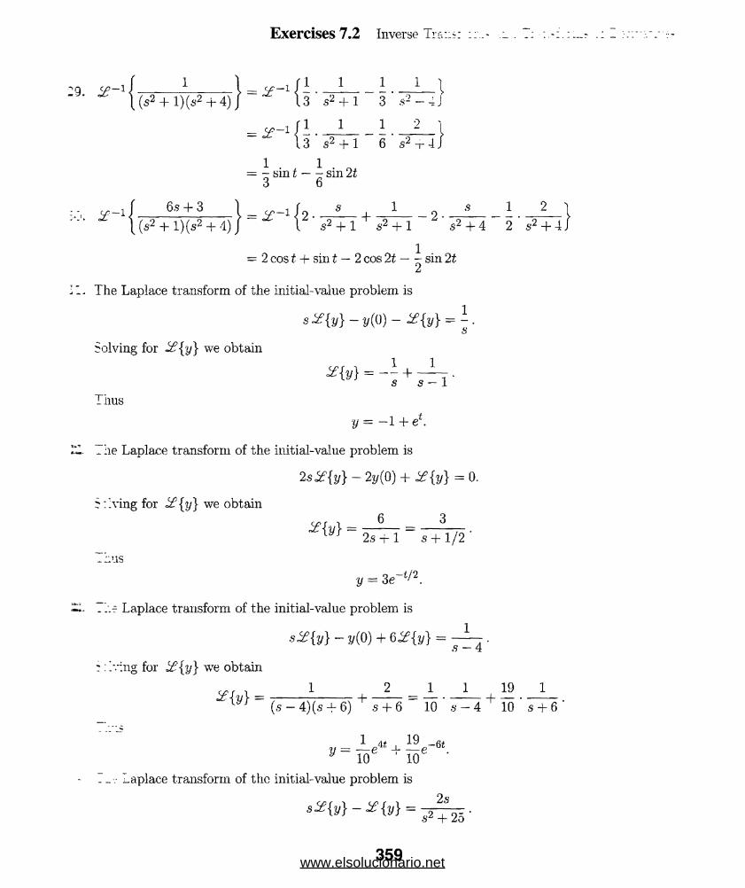
Exercises 7.2 Inverse Tra::?:
y - i / ______ 1______ \ = * - i ( I . _ J _____I . _ i _ l[ (s2 + l)(s2 + 4) J 13 s2 + l 3 »2- 4 j
= ___ -____ - • -7- ___i13 s2 + 1 6 s2 -r 4 J
1 • 1 . «= - sm t- - sin
3 6
ff-i I 6.9 + 3 \ _ ^>-112 ____£___ |___ ____ 9
| (s2 + l)(s2 + 4) J I s2 + l s2 + l "
.9 1 2
s2 + 4 2 s2 + 4.
= 2 cos i + sin t — 2 cos 2i — ^ sin 2iZj
The Laplace transform of the initial-value problem is
Solving for i?{y} we obtain
.9 5 — 1
Thus
! / = - l + e‘ .
The Laplace transform of the initial-value problem is
2s i f {y} - 2y(0) + i?{y} = 0.
5:’;ving for if{y} we obtain
v r , 1 6 _ 3
~ 25 + 1 ~ 5 + 1 / 2 ‘
7::us
y = 3 e-t'/2.
T..- Laplace transform of the initial-value problem is
- !/(0) + = 1.9 — 4
' :lv:ng for Z£{y} we obtain
oj f 1 1 2 1 1 19 1T u r. ^ + m = 77; ■ 7 + ^(.9 —4)(s + 6) 5 + 6 10 5 — 4 10 s + 6 -
v = — e4t -1- — e~6i y 10 ' 10 '
Laplace transform of the initial-value problem is
^ « - * W = ? T 25-
359www.elsolucionario.net

Exercises 7.2 Inverse Transforms and Transforms of Derivatives
? living for Z£\y\ we obtain
vr _ 2s 1 1 1 s 5 5lM i ~ /„ , oc> — 10 ' „ i 19 „2 I o c '* ' io(s - l)(s2 + 25) 13 s - 1 13 s2 + 25 13 s2 + 25 '
TI'/.is1 1 0
i, = i3 '’‘ “ T3COs5t + S 5inM-
Ti.f Laplace transform of the initial-value problem is
s2 {y} - n/(0) - 1/(0 ) + 5[<Jf{»} - y(o)] + 4if{»} = o.ving for l£{y} we obtain
s + 5 4 1 1 1
s2 + 5s + 4 3 s + 1 3 s + 4
Tims^ —t 1 —At
y = ? ~ r •
36. The Laplace transform of the initial-value problem is
s2 2{y} - sy(0) - </(0) - 4 !.S Z{y} - 3,(0)] = 6 35- 3 5+1
5 T.ving for 1£ {y} we obtain
< rr l 6 3 5 - 5^{y} ~~ 77.— 5T772--7^ ~ 77TTu72 +(s — 3)(s2 — 4s) (s + l)(s2 —4s) S2 — 4,s
5 1 2 3 1 11 1+ ~r~r
2 5 5-3 5 5 + 1 10 5 - 4
Tims® -> Sf 3 11
V = 2 ~ 2c ~ r + K e ■
\ The Laplace transform of the initial-value problem is
2s2X{y} - sy(0) + % {?/} = -n
s2 + 2 ‘
jiving for i f {y} we obtain
2 105 10s 2 2
(s2 + l)(s2 + 2) 52 + l S2 + l s2 + l s2 + 2 ’
Thus
y = 10 cos t + 2 sin t — a/2 sin \[21.
35. The Laplace transform of the initial-value problem is
=,2 y /„ i _i_ 0 y/,A _ ls ^ { y } + 9^{y} = —
360www.elsolucionario.net
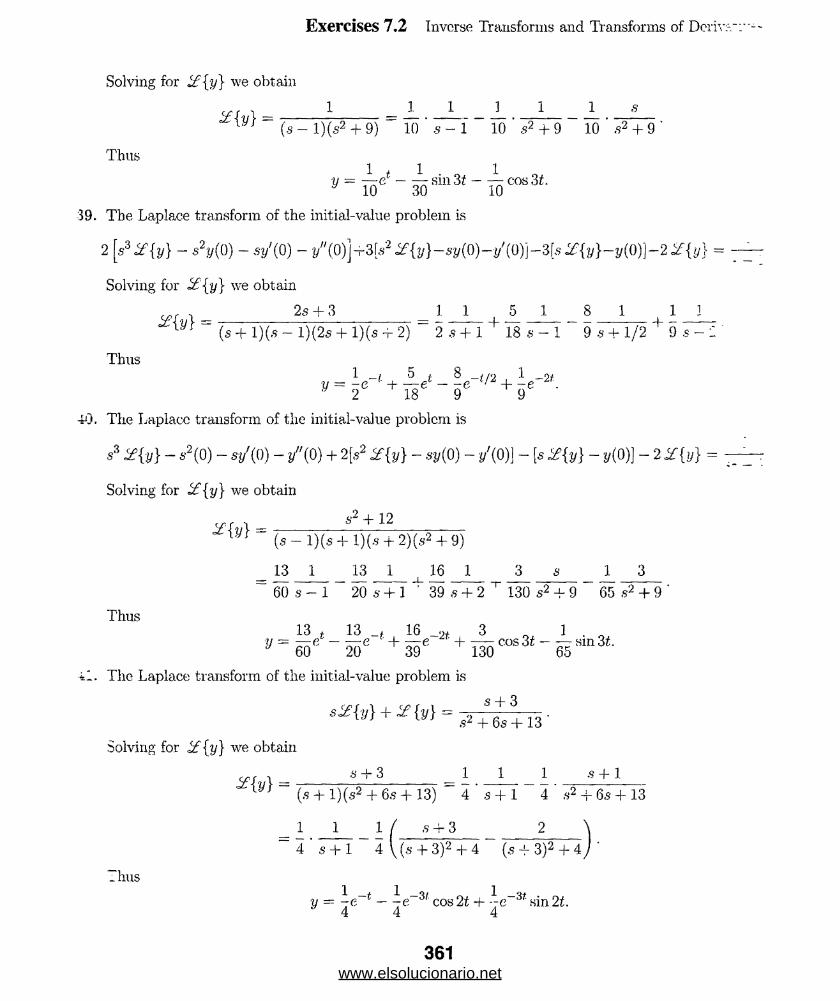
Exercises 7.2 Inverse Transforms and Transforms of Dcr
1 1 1
Solving for if{y} we obtain
0 - l ) ( s 2 + 9) 10 s - l 10 52 + 9 10 52 + 9
Thus
39. The Laplace transform of the initial-value problem is
2 [s^{y } - s2y(0) - V (0 ) - /(0)]^3[52^{y}-5|/(0)-y,(0)j-3[5^{y}-y(0)j-2y{|/-}
Solving for i f {y} we obtain
, 2s+ 3 1 1 5 1 8 1 1 I- f~. 7 i\ /Z iV/oT T T\Fr - o TTT + To 7 T ~ n T i~7n +(s + 1)(*9 — l)(2s l)(s t 2) 2 .? +1 18 s — 1 9-9 4" 1/2 9 s — _
Thus1 _/ 5 * 8 —i/‘> 1 —9
V~ 2 e + l8 e' - 9 e " + 9e "•
■4*3. The Laplacc transform of the initial-value problem is
,93 i?{y} - s2(0) - sy'(0) - y"(0) + 2[s2 if{y} - 6>y(0) - y'(0)] - [s i?{y} - 2/(0)] - 2 if{y} =
Solving for i f {y} we obtain
52 + 12
(s - l)(s + 1)(,9 + 2)(s2 + 9)
13 1 13 1 16 1 3 s 1 3
60 s - l 20 s + 1 ‘ 39 .9 + 2 130 52 + 9 65 52 + 9 '
Thus13 f 13 _t 16 _2f 3 0 1 . ,
V = 60e - 20e + 39 + 130 C°S 65Hln
=1. The Laplace transform of the initial-value problem is
s -J- 3s2{y} + ¥{y} =
32 + 6s +13
Solving for .if {y} we obtain
5+3 1 1 1 5+1*{v} = (5 + 1)(52 + 65 + 13) 4 s + 1 4 52 + 65 + 13
1 1 1 / 5 + 3 2 \
4 5 + 1 4 \ (5 + 3)2 + 4 (5 + 3)2 + 4/
Thus1 _f 1 _oy 1 _94
y = -e — -e cos 2 t + --e sin2f.4 4 4
361www.elsolucionario.net

Exercises 7.2 Inverse Transforms and Transforms of Derivatives
i2. The Laplace transform of the initial-value problem is
- s ■ 1 - 3 - 2[.s %{y} - 1] + 5 %{y} = (a2 - 2s + 5) %{y} - 3 - 1 = 0 .
Solving for 0£{y} we obtain
s +1 a - 1 + 2 s- 1 2
s* — 2 s + o (s — l)2 + 22 (s — l)2 + 22 (s — l)2 + 22«2
Thus
y = ef cos 2f + e* sin 21.
43. (a) Differentiating /(f) = teat wc get /'(f) - ate0* + eat so ££{a,teat + eat} ■ ■ s^£{teat}1 where
have used /(()) = 0. Writing the equation as
a¥{teat} + X {ent} = sl£{teai}
and solving for ££{teat} wc get
2{teat} = — X{eat} = 1s — a 1 J (s — a)2
(b) Starting with /(f) = t sin ki we have
f i t ) — kt cos kt + sin kt
f i t ) = — k2t sin kt 4- 2k cos kt.
Then
^ { —k2t sin t + 2k cos kt} = s21£ {f sin kt}
where we have used /(()) = 0 and /'(0) = 0. Writing the above equation as
—k2l£{t sin kt} + 2k 0£ {cos kt} = s2 Z£{t sin kt,}
and solving for ^f {t sin kt} gives
2k (rc . , 2k s 2ks^{tsmkt} = ~2 —^ ^ ( COskt} - ^2 ^ 2 - (.,2 + *2)2 *
44. Let /i(f) = 1 and /2(f) = j ^ J, f ^ 1 Thcn ^ { f^ t )} = % {/2(f)} = 1/s, but /i(f) ^
45. For y" — Ay' = 6e3t — 3e~( the transfer function is W(s) = l/(s2 — 4s). The zero-input respon-
"<*> - ^ “ {i- ;■- i ' 7 ^ } - i - ~ /1’
362www.elsolucionario.net

Exercises 7.3 Operational Properties
and the zero-state response is
6 3yi{t) =5£ 1-
[ (s — 3)(-s2 — 4s) (s + l)(s2 — 4s) j
= i f -1 <f — __-______ 2 i 5 1 3 1 ]120 s — 4 s — 3 4 s 5 s + 1J
27 a* n ~ 5 3 _t
“ 20e “ 2e + I “ 5C '
From Theorem 7.2.2, if / and f arc contiimous and of exponential order. = sF(s) — /
From Theorem 7.1.3. = 0 so
lim [sF(s) - /(0)] = 0 and lim F(s) = /(0).o *\JG & *
For /(t) = cos Ai,
lim sF(s) = lim s 9 * 9 = 1 = /(0).S->O C V ’ 8 —>OC A>2 £ 2 J \ /
<>pwati<?na| Frop«rties I "irf:;'• j' -V \ s' L s' - : - ~... '' 2 ~ “ •'* 5 '•...\ *“v” » *“ “j
s. i:v ;•£;
- (s _ 10)2
* { *■ * } - j r t w
= ( J W
{ t(ef + e!t) | = if{ le 2< + 'lteM + te4'} = ^ _ ,-,,2 , (s _ 3 ) 2 1 (s _ 4 ) 2
jf {e2«(f - 1)2} = i f {tV> - 2(e2‘ + e21} = ^ - 4 ^ - + 1
2 1+
(s - 2)3 (s - 2)2 s - 2
= (s _1)2 + 9
jf{e-2f cos4f) = -—*■ J (s + 2)2 + 16
363www.elsolucionario.net

Exercises 7.3 Operational Properties I
9. J. {(1 — et + 3e ) cos 5#} = i f {cos bt — ef cos 51 + 3e 4< cos 51}
_ $ 5 — 1 3 (5 4- 4 )
,s'2+ 25 (s — l)2 + 25 (s + 4)2 + 25
9 4+
3 (s - 3)2 (s - 3)‘2 + 1 /•;10. if je 3f 9 — At + 10s i n ^ | = i f |9e^ — A te + lOe^sin^|= -
11 -/_1( - \ = i f —1 / — - 1 = - f 2p~2/~ I ( « + 2)3 / * \ 2 (5 + 2)3 / 2
“ l ( ^ - l ) 4 J 6 ^ l ( 5 - l ) 4 / 6 t e
13- - 1 + 10} = { (« - 3)2 + 12 } = ^ Sin*
14' * ‘ { S2 + 2s + o } = ,y ^ 2 (s-H I)2 -H 22} = 2e >Sm2t
- i f S \ _ V - l j 5 + 2 1 1 ___ —2t ____ r >- 2t.15. i f M —r-- ----- f = i f < -----r~— — 2----—~— -k > = e “ cost — 2e sintls 2 + 4s + 5j \(5 + 2)2 + l 2 (s + 2)2 + l2 J
16, —-V~ J— } = i f - 1 / 2-— r2 — ~ — 3 } = 2e_,%cos51 — ^e_3tsinof 152 + 65 + 34 j \ (s + 3)2 + 52 5 (s + 3)2 + 52 J 5
( W ) =' i A * 5 ^ 1 ■,0 r - i f 25-1 1 t, , [5 1 5 4 3 2 ) -f -t19. i f < -K-,— — so > = £ \----o --- —r — 7---tt? — - 7-----To r = 5—t—5e —Ate —
5 (5 +1) J \s 5 5 + 1 (5 + 1)2 2 (5 + l )3 J
o0 y - J (6~ + 1I 2l = ^ - 1/ _____________ -___+ 1 ___ -__ \ = f ( - x _ t 2e-2t + -t3(-'2tJ- x l ( 5 + 2)4/ x \(5 + 2)2 (5 + 2)3 + 6 (5 + 2)4j tC te 6
21. The Laplace transform of the differential equation is
15if{y} - y(0) + 4if{y}
5 + 4
Solving for if{y} we obtain
1 2V\ = 7 . +
(5 + 4)2 s + 4 ’
Thus
y = te~if’ + 2e~4t.
364
IO I C
O
www.elsolucionario.net

Exercises 7.3 Operational Properties I
22. The Laplace transform of the differential equation is
s (s — l)2 '
Solving for i f {y} we obtain
v r i 1 . 1 1 1 1° £ { y } — ~ ( -------------- T T 1 " 7 -------------- T y T — ----------------!--------------------7 +
s(s — 1) (s — l)3 s s — 1 (s — l)3 ’
Thus
y = - l +e‘ + itV .
23. The Laplacc transform of the differential equation is
s2if{y} - <*(()) - y'(0) + 2[sX{y} - j,(0)) + ^{j/} = 0.
Solving for ?£{y} we obtain
<c r 1 s + 3 1 2£ iv} = TTV^v} = TTT +(s + l)2 s 4- 1 (s + l)2 ‘
Thus
y = e-* + 2te~l.
:4. The Laplace transform of the differential equation is
S2 X { y ] - Sy(0) - y'{0) - 4 (S X { y ) - y(0)] + iZ {y ) = 6(s-2) 4 *
Solving for 2 {?;} we obtain ¥{y} = ^ 6 . Thus, y = ^ t 5e2t.
25. The Laplace transform of the differential equation is
s2 X{y} - 51/(0) - j/(0) - 6 [ ^ { y } - s,(0)] + 92{y} = i .Solving for i?{y} we obtain
. 1 + s 2 2 1 1 1 2 1 10 1s2{s - 3)2 27 s 9 s2 27 s - 3 9 (s - 3)2 '
Thus 2 1 2 v 10 «V = — 4- - t--- e6t H---te .* 27 9 27 9
2o. The Laplace transform of the differential equation is
s2 %{y} - sy(Q) - ?/(0) -4[s¥{y} - 2/(0)] + 4¥{y} = .s
Solving for if{y} we obtain
,rr . .s5 — 4.s4 4- 6 3 1 9 1 3 2 1 3! 1 1 13 1 y} = — 7ZT - 7 7 + o72 + 7 3 + 774 + 7l(s - 2)2 4 s 8 s2 4 s3 4 s4 4 s — 2 8 (s - 2)2 ‘
www.elsolucionario.net
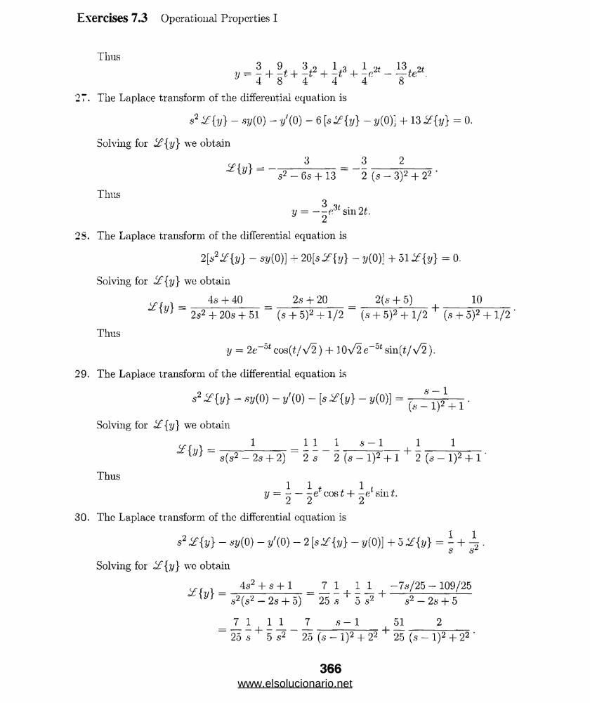
Exercises 7.3 Operational Properties I
Thus3 9 3 9 1 o 1 <>/ 13 ->t
+ + ? - ¥ te
27. The Laplace transform of the differential equation is
s2 <£{y} - sy(0) - y'(0) - 6 \s%{y} - y(0)] + 13 2{y} = 0.
Solving for ££{y} we obtain
Vt —,s2 - C)5 + 13 2 (5 - 3)2 + 22 '
Thus3 v
y = — (r sin 21.J 2
2S. The Laplace transform of the differential equation is
2|V2if{y} - 5y(0)] + 20[s%{y} - y(0)j + 51 if{y} = 0.
Solving for i f {y} we obtain
(„f 1 4s + 40 25 + 20 2 (5 + 5 ) 10i on,, i ci („ i C\2 i i/o i rt\2 i 1 /o2s2 + 20s + 51 (s+ 5)2 + 1/2 (5 + 5)2 + l/2 (5 + o)2 + 1/2 '
Thus
y = 2e~ot cos(t/\/2) + 10 V 2 e~ot sin(t/y/2-).
29. The Laplace transform of the differential equation is
- s»(°)-J/'(0) - -»(0)] = 4 1(«-1)2 + r
Solving for if{y} we obtain
f. r , 1 1 1 1 5 -1 1 12 o» 1 o \ o o ( „ i \ 2 1 1 <15(s2 - 2s + 2) 25 2 (5 - I)2 + 1 2 (5 - l)2 + 1 ‘
Thus1 1 * 1 1 ■y = - — -e cos t + -e sm t. z z z
30. The Laplace transform of the differential equation is
s2 %{y} - 5y(0) - y'(0) - 2 [s£{y} - 2/(0)] + 5 %{y} = 7 + - •s &
Solving for if{y ) we obtain
^ r 4a’2 + 5 + 1 _ 7_ 1 ^ 1 1_ , -75/25 - 109/25
^ 52(s2 — 2s + 0) 25 5 ' 5 s2 T 52 — 25 + 5
7 1 1 1 7 5-1 51 2<-»- I- _ 7 TTo ! 4"25 5 5 52 25 (5 - I)2 + 22 25 (5 - I)2 + 22 '
366www.elsolucionario.net
Exercises ".5
Thus
31. Taking the
7 i 7 . -
V = 25 + 5t '2 S ' ' “ '- '~ ^ :
obtain
Tercnuai eq:iaT:>_>:; a::;:
Z{y"}+ ¥{2y '}+ Z{y} = 0
sz!£{y} - sy(0) - y'{0) - 2s if{y} - 2y(0) + if{y} = 0
,92if{y} — cs — 2 + 2s if{y} — 2c + i f {y} = 0
(s2 + 2,9 + 1 j i f {y} = cs + 2e + 2
t^r i cs 2c — 2~£{y} = 7 ~ . +(.9+1)2 ( ^1-2
_ ^ s _ + l - l . 2c * 2
(s + l)2 ■ (s - 1 -
c c + 2
s + .1 (s + 1)
Therefore.
y{t) = c% 1{j^T [} + (c + 2) ^ ^ ( I+ l ) 2} = CC t + (c + 2)te
To find c we let y(l) = 2. Tlion 2 = cfi-1 + (c + 2)e_1 = 2(c + l)e_1 and c = e — 1. Thu.'
y(t) = (e - l)e-' + (e + l)te_ i.
:2. Taking the Laplacc transform of both sides of the differential equation and letting c =
obtain
^ { / } +^{8y'} + i f {20 y} = 0
s2Z{y} - y'{0) + 8.9 2{y} + 20if{y} = 0
s2if{y } — c + 8.9 i f {;{/} + 20if{y} = 0
(<92 -I- 8.9 + 20) i f {y} = c
2(v\ = s2 + 8s + 20 (* + 4)2+4
Therefore.
1 { Is + ' i f +'4 } = I C" 41 ™ 2t ~ C,e 4,Sill2('
367www.elsolucionario.net

Exercises 7.3 Operational Properties I
To find c we let y'(ir) — 0. Then 0 = y'(^) = ee'"47r and c = 0. Tims, y(t) = 0. (Since
differential equation is homogeneous and both boundary conditions arc 0. wc can see immedia"
that y(t) = 0 is a solution. Wc have shown that it is the only solution.)
33. Recall from Section 5.1 that mx" = —kx — fix'. Now m = W/g — 4/32 = | slug, and 4 = 2-
that k = 2 lb/ft. Thus, the differential equation is x" + 7x! + 16x = 0. The initial conditions
,r(0) = — 3/2 and 3/(0) = 0. The Laplace transform of the differential equation is
+ -s + 7 s«C{x} + ^ + 16if{:r} = 0.
Solving for we obtain
-3s/2 — 21/2 3 .s + 7/2 7/L5 \/l5/2
s2 + 7s + 16 2 (,<? + 7/2)2 + (\/l5/2)2 10 (5 + 7/2)2 + (vT5/2)2 ‘
Thus
3 _7(/2 7\/l5 _7f/2 . x = — -e 1 cos—— t ----- e ' sin—— i.
jl.- Z JL U Zi
34. Tlic differential equation is
S + 2077 + 20°1 = 150' «(°) = f/(° ) = °- at* at
The Laplace transform of this equation is
I ROs2£{q} + 20sX{q} + 200^{q} = .
Solving for i f {<7} we obtain
150 3 1 3 s +10 3 10%{q} =
s{s2 + 20s + 200) 4 s 4 (s + 10)2 + 102 4 (s + 10)2 - 1()2 ’
Thus
q(t) = 7 — \e~U)t cos 10i — 7e_ 10*sinl0f w 4 4 4
and
i(t) = </(/•) = 15e_10/sin lOf.
35. The differential eciuation is
| f + 2A § + c ^ = § , ?(0 )= , '(0 )= 0 .
The Laplace transform of this equation is
s2X{q} + 2As¥{q} + u>22{q} = -L/ 8
orEq 1
(s'2 + 2 As + w2) i f {<?} = - .
368www.elsolucionario.net

Exercises 7.3 Operational Properties I
_ E0 (1 /u2 [1/lv2)s + 2X/lv2\ = Eq f l s + 2A \
W L \ a s2 + 2As 4- (v2 ) Lu2 \x s2 + 2Xs + (v2) '
For A > u> we write s'2 + 2A-s + J 2 = (s + A)2 — (A2 — u;2), so (recalling that io2 — 1/LC:
opr p* s-i( 1 s + A A \X\_q) = E0C y- - (s + A)2 _ ( A2 _ u;2) - (s + A)2 -(A2 -c.’2) J '
Solving for and using partial fractions we obtain
Thus for A > u
<?(*) = 1 — e I cosh \/A2 — oj2 t —A
: sinh \/ A2 — ll?2 t
For A < w we write s2 + 2As + iv2 = (5 + A)2 + (a;2 — A2) , so
%{q} = £*)C^- - (s + A)2 + ^ .2 _ A2) - (S + A)2 + (W2 _ A2) ) •
Thus for A < tv.
q(t) - E0C 1 _ e At / cos J w2 _ A2 f ---^ sin v/u/2 — A2\ v w2 — A2 J _
For A = cv, s2 + 2A + J 2 = (s + A)2 and
AEp 1 £ p / l / A 2 1/A2 1/A N J5b / l 1_____________
L s(.s + A)2 L y s s + A (s + A)2/ LA2 s + A (s + A -
Thus for A = ui,
lo. The differential equation is
The Laplace transform of this equation is
q(t) = EqC(i — e ^ — At e .
Rs2{q} + ^ 2 { q } = E o j ^
Solving for i£ {5} we obtain
=£ 0<? Eq/R
{s + k)(RCs + l) {s + k){s + l/R C ) '
When 1 /R,C / k we have by partial fractions
r„ f ■ E0 ( l / ( l /R C - k ) 1/(1 /RC-k)\ E0 1 ( 1
i?, V s + fc
Thus
«(*) =
s + 1 jR C J R 1 IR C -k\ s + k s + I IRC I '
369www.elsolucionario.net

Exercises 7.3 Operational Properties I
When l/R C = k we have
Thus
<sr i _ ^ 1(? ! H (s + fc)2 '
9W = f f c - “ = f t e - ‘/BC
38 . if{e2“* (f - 2)} = i f {e-(t_2> *1/ (* - 2)} = -+ 1
39. if{t9i(t-2)} = ^ { ( i - 2 ) ;W ^ - 2 )+ 2 ^ ( i- 2 ) } = ^<5 ^
Alternatively, (16) of this section in the text could be used:
/ 1 2'i f{t V (t - 2)} = e~2s ¥ {t + 2} - e_2s + -) •
Q — <S 1
40. if{(3t + 1)% (i — 1)} = 3if{(£ — I ) 3?/ ( t— 1)} + 4 i f { ^ (t — 1)} = '-— + ~6 tS
Alternatively, (16) of this section in the text could be used:
if{(3 i + 1) °U- (t - 1)} = e-*Z{3t + 4} = e~* ( ^ ^ ^ ) •
S€~vs41. i f {cos 2 t LU(t — tt )} = if{cos2(i — x)''U(t — 7r)} = 2 t
Alternatively, (16) of this section in the text could be used:
if{cos2t £W (t - 7r)} = e-7™ i f {cos 2(t + tt)} = e~xs if{cos2t} = e~
42. v u - z w - - ~ " ' 227 J ~ y 27 " V 27J s2 + l Alternatively, (16) of this section in the text could be used:
if-fsint (t — ^ } = e~vst2 i f (sin (t + ^ 1 = e~™/2 ^{cosi} = e
e~*a45. i? 1 < ~2 > = sin(i — 7r) ~V, (t — tt) = — sint °U (t — tt)
■fi
s2 + 4 ’
-tt.s/2 *,S2 + 1
370
www.elsolucionario.net
Exercises 7.3 Operational Properties I
C / ? - l . se -Trs/2
4 8 . i f
4 9 . ( c)
,s’ 2 + 4 j
iSiil' p - 2s
= i f
= if- x
•(-a
= ~m (*- 2) “ (t - 2)^ (* - 2) + et_2fiM (t - 2)
j =<U(t- 1) - e " ^ 92 (* - 1)
2*s 2 s p—2<s
50. (e) 51. (f) 52. (b) 53. (a) 54. (d)
oo.
56 .
35.
59.
i f {2 - 4 s?/ (* - 3)} = - - -e~3ss s
if { l —°1l (t - 4) +S1Z (£ - 5)} = - - — + —s s s
%{t2cU (t- l)} = if{ [ ( i- l)2 + 2t- l] °U (t- 1)} = i f j [(£ - l)2 + 2(t — 1) + l] M (t- 1)}
/ 2 2 1\
- ( ? + P + l ) e
Alternatively, by (16) of this section in the text,
2 { t2 %\t - 1)} = e-s i f { f 2 + 2t + 1} = eT* ( 4 + 4 + - ) •\ S S S /
se-37rs/2i f | sin t ~U ~ ) } - 4 cos t
s2 + 1
%{t-t<U{t-2)} = 2 { t - ( t - 2) W (t - 2) - 2oil (t - 2)} = \ ^qA qZ
oO. i f {sin i — sinf °U. (t — 27r)} = i f {sinf — sin(f — 2tt) cU (t — 27t)} =
sA s*
1
s
—2 tts
s2 + 1 S2 + 1
51. if{ /(f)} = i f {9/ (t — a) — % (t — b)} =e-as e-b*
1 e~52. + + — + — + ^ + . — ,
6‘ s s s 1 — e~s
53. The Laplace transform of the differential equation is
s i f {y} - y(0) + if{y}
Solving for i f {y} we obtain
.s s + 1
371www.elsolucionario.net
Exercises 7.3 Operational Properties I
Tims
y = 5 ’V(t — 1) — 5e-^-1) 'tt (t — 1).
64. The Laplacc transform of the differential equation is
So'-ving for ^{y} we obtain
x{v} =2e~H
■s(s + 1) .9(5 + 1) ,9 .9 + 1— 2e"
s s + 1.
Thus
y = l- e ~ i - 2 [1 - - 1).
65. The Laplace transform of the differential equation is
S y{8,} - 1,(0) + 2 Z{y} = I - e - £ ± i
Solving for
•*{»} =
Tims
we obtain
1 $ + 1
,92 (,9 + 2) ,92 (.9 + 2)
11 1 1 1 1_ _ _ I _'4 ,9 T 2 ,92 ■ 4 .9 + 2
11 1 _1
4 s + 2 ss
1 1 1
» — i + 5t + i « _ a - L4 2
66. The Laplace transform of the differential equation is
S 2{y }-3y (P )- ,/(p )+ 4 2 { y} =1 e
Solving for ¥{y} we obtain
1 — s
s(s2 + 4)
I l l s 1 2
s(.92 + 4) 4 .9 4 .92 + 4 2 s2 + 4
1 1
4 s
Thus1 1 „ 1 • „y = - — - cos 21 — - sm 2t — 4 4 2
^ - i c o s 2 ( « - l ) ^ ( i- 1 ) .
6 7. The Laplace transform of the differential equation is
s2 if{y} - *2,(0) - t/(0) + 4 ^{i,} = .s* + 1
Solving for if{ y} we obtain
Thus
VY = 8 + e_27r,s
y — cos 2t +
.s2 + 4
'1
1 1 1 2
.3 s’2 + 1 6 s2 + 4.
sin(t — 2tt) — - sin2(£ — 2-tt) o u
— 27r).
1 1 1
4 s + 2.
1 s ~
4 s2 + 4.
372www.elsolucionario.net

Exercises 7.3 Operational Properties
The Laplace transform of the differential equation is
s2 { j,} - «y(0) - w'to) - 5 [« i f {»} - »(())] + 6 X{y\ = e— .
Solving for ¥{y} we obtain
vy — e
= e
—s +1
s(s — 2)(s — 3) (s — 2)(.s — 3)
1 1 1 1 1 1 1 1+
Thus
V L6 2
6 s 2 s - 2 1 3 s - 3 j s - 2 s - 3
U{t - 1) - e2t t- e3*.3
IS
S2^ f o } - S<,(0)-y'(0)+ .S%} =g—K8 e-271"*
Solving for i f {t/} we obtain
i% } = e"™n
s s2 + 1— e—2tt$
s s'2 + 1+
s2 + l
Thus
y = [ 1 — co s(t — 7r)]°M(i — tt) — [1 — cos(it — 2ir)]^(i — 2;r) + sin t.
is
1 e~2s e~*3 e~i>ss2 %{y} - 3J/(0) - l/(0) + 4[s if{t/} - y(Q)] - 3 &{y] =s s
+
Solving for if{y} wc obtain
!£{v\ = - - - - _-___ l - _-__XJt 3 s 2s + l ' 6s + 3
,—4.9
-2s1 1 1 1 1 1
+3 8 2 8 - 1 6 s -f 3
1 1 1 1 1 1 +
3 s 2 s -j- 1 6 s + 3+ e.—G.s- 1 1 1 1 1 1
L ilUS
1 1 -t 1 -3ty = - - -e f + -e M J 3 2 6
1 _ i e-a-2) . I^-3(£-2)3 2 6
I _ i p- ( < - 4) , I p - 3( / - 4)' 3 2 ' 6 '
3 s 2 s + 1 6 s + 3J
ni(t- 2)
1 ....... n«(t-6)._ _ i _ p-3(i-0)3 2 6
7 -call from Section 5.1 that nix” = —kx + f(t). Now m = W/g = 32/32 - 1 slug, and 32 =
r: that k = 16 lb/ft. Thus, the differential equation is x" + 16a1 = f(t). The initial conditions
j) = 0, a/(0) = 0. Also, since
m =201, 0 < t < 5
0, t > 5
373www.elsolucionario.net
Exercises 7.3 Operational Properties I
and 201 = 20(f — 5) + 100 we can write
/(f) = 201 - 20f ;l/(i - 5) = 201 - 20(f - 5)9/(f - 5) - 100 sU{t - 5).
The Lapla,ce transform of the differential equation is
9 <7"r 1 -in <7~f 1 2 0 2 0 1 0 0+ 16<£{;?:} = -s--- s - e ----e 0i.
s $*•
Solving for l£ {;r} we obtain
20 20.S2 (S‘2 + 16) S2 (.S2 + 16)
5 1 5
e-°* -100
s(s2 + 16)
_ e-5^ _ ^ I _ ^ S ■1 s2 16 s~ +16/ 6 \4 s 4 6'2 + 16
Thusf1 ‘S 1 rOtt s: n^ (f - 5) - ^ sin 4(f - 5), (f - 5) - ^ cos 4(f - 5) ^ (f - 5
= ~t — sin4f — ^H/ (f — 5) + sin 4(f — 5) JU(t — 5) + ^ cos4(t — 5) ,Jtl(t — 5).4 16 4 16 4
72. Recall from Section 5.1 that nix" = —kx + /(f). Now rn = W/g - 32/32 = 1 slug, and 32 = .
so that k = 16 lb/ft. Thus, the differential equation is x" + 16:r — /(f). The initial conditions
,r(0) = 0, ^(O) = 0. Also, sincef sinf, 0 < t < 27r
^ ~ { 0r t > 2tt
and sin f = sin(f — 2tt) we can write
/(f) = sinf — sin(f — 27ryu(t — 2tt).
The Laplace transform of the differential equation is
s2 } + 16 {:r} = -1
Solving for if{x} we obtain
2 W =
s2 + 1 s2 + 1
1
(s’2 + 16) (s2 + 1) (s2 + 16) (s2 + 1)
-1/15 1/15
S2 4- 16 s2 + 1
-1/15 1/15
s2 + 16 s2 + 1
,—2irs
- 2 tts
Thus
x(t) = sin4f + ~ sinf + -^-sin4(f - 2tt)^ (£ — 2tt) — sin(f — 27r)^(f - 2?r)DU 10 DU 10
— sin4f + y= sinf. 0 < £ < 2tt
0, f > 2tr.
374www.elsolucionario.net

Exercises 7.3 Operational Propel'':
The Laplace transform of this equation is
'3. The differential equation is
2.5 ~ + 12.5# = 5 (£ — 3).LtC
8 {q} + 5 {q} = -e~3a.s
Solving for ¥{q} we obtain
x {^} = _ L e-3» = ( ' ? . ! _ ? . -J— '] e_a's.s(s + 5) \5 s 5 s + 5/
Thus
q(t) = \ 'JU(t — 3) — JU(t — 3).O 0
'4. The differential equation is
10 ^ + 10q = 30el - 30enli(i - 1.5). dt
The Laplace transform of this equation is
3 3e‘-a , 5,s2{q ) - ® + y {?} = — - J— e
Solving for ¥{q} we obtain
_ / 3\ 1 3 1 v, L5 / 2/5 2/5 \
- ( « - 2 j ■ IT T + 2 ' 7 ^ 1 - 3c + e ■
Thus
?(<) = (so - 5) + 2e‘ + j* 1-3 (<rC-’-5> - ei-5{i-i.s)) CU ( ( _ L 5 ) .
"5. (a) The differential equation is
~ + lOi = sin t + cos (t - , '<(0) = 0.
The Laplace transform of this equation is
I „ „ - 3 tt.s / 2
4y {i} + io * W = ? T T + ^ T r .
Solving for i?{/} wc obtain
= ----- •------ -I------------ 3«.s/2W (s2 + 1 )(s + 10) (s2 +1 )(s + 10)
1 / 1 s 10 \ 1 / -10 10s10 \ 1 / -10 , 10s 1 \ ;
101 Vs + 10 s2 + 1 + s2 + 1J + 101 \s + 10 1 s2 + 1 + s2 + l j ^
375www.elsolucionario.net
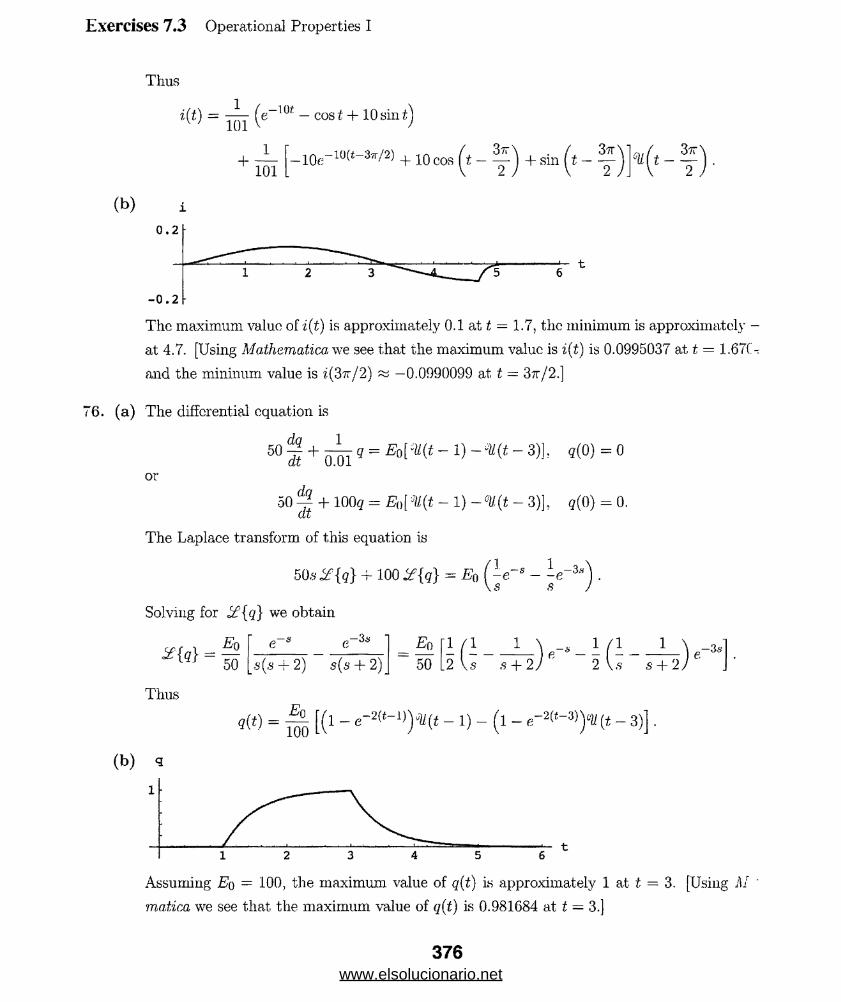
Exercises 7.3 Operational Properties I
Thus
i(t) = -!- (e 10f — cost + lOsin*)
+ m
- 0 . 2
The maximum value of i(t) is approximately 0.1 at t = 1.7, the minimum is approximately -
at 4.7. [Using Mathematica we see that the maximum value is i(t) is 0.0995037 at t = 1.67C
and the mininum value is i(37r/2) ~ —0.0990099 at t = 37t/2.]
76. (a) The differential equation is
50Tt + oTil9 = Ea[* {t ~ !) ~M{t ~ 3))' 9(c) = 0
50 + 100q = £„( :ll(t - ! ) - « ( ( - 3)], 5(0) = 0.
or
The Laplace transform of this equation is
50s i f {9} + 100 %{q\ = Eq (- e~s - V 3*Vs s
Solving for if{#} we obtain
-3s
Thus
s(s + 2) s(s + 2)
q{t:> = W0 K 1 _ - 1) - ( l - f (t - 3)] •
Eo
50
1 / l 1 / I
2 Vs s + 2-3 s
( b ) q
Assuming E q — 100, the maximum value of q(t) is approximately 1 at t = 3. [Using AI
matica we see that the maximum value of q(t) is 0.981684 at t = 3.]
376www.elsolucionario.net

Exercises 7.3 Operational Properties I
Tlie differential equation is
Taking the Laplace transform of both sides and using y(0) = y'(0) = 0 we obtain
s4X{y} - sy"(0) - / '(0 ) = H i ( i - .
Letting y/r(0) = ci and y"'(0) = C2 we have
Ci C2 , wo 1
so that
, . 1 9 1 o 1 M)oy(x) = -cix 4- -c2rr‘ + — —
2"‘~ ' 6
To find ci and c*2 we compute
24 E l ‘H )//, N 1 wo
.(/ (x) = c 1 + c2a: + - — a:2 — (a: — - ) %( a; — —
andtwo
a:
Then y"(L) = y"'{L) = 0 yields the system
1Cl + <**+ 5 1 7 i 2 - ( i
3 wqL2
= Ci+C2i"-8“g r = 0
wo /L\ 1 wo-t n
°2 E I\ 2) 02 2 E l
Solving for c.\ and we obtain c\ = I wqL2 j E l and C2 = —\w$ L /E I. Thus
y(x) =wo
E l1 T2',-2 16LX
_ he differential equation is
E I& * = -°U(X ~ 2Xr/3)].
Taking the Laplace transform of both sides and using y(0) = y'(0) = 0 we obtain
- i/ (0 ) - / '(0 ) = H I (e-i»/3 _ e-21*/3) .
Lotting yw(0) = ci and y’"{0) = C2 wc have
^ = ? + ? + I ? ( e' i , / 3 - e-2W3)
377www.elsolucionario.net
Exercises 7.3 Operational Properties I
so that
1y(x) - ^c\x2 + ^C2X6 + -
1 ,3 1 tiu
2“L~" ' ‘ 24 E I
To find ci and c2 we compute
t t / \ i i ^ y (x) = ci + C2 X + - —
andu?0/// / \ , u
y (s) = c2 + — LW L* - 3 W l
2L\ / 2L
Then y"(L) = ym(L) = 0 yields the system
r , 1 Cl + C2i + - — = ci + co.L + I = 0
Cowq \2L L
e I 3J
6 E I
1 WqL
3 E I= 0 .
Solving for ci and c2 we obtain ci = \ w§L2 j E I and c2 = —\wqL /E I. Thus
E I \12
79. The differential equation is
24
dAy _ 2w{)Oil --7 — -“—
dx4 L
Taking the Laplace transform of both sides and using y(0) = r/(0) = 0 we obtain
2wqsi Z{>j}-sy"( 0 )- / ' ( 0 ) =
Letting y"(0) = ci and y"'(0) = c2 we have
Cfir x ci c2 2 w q
+ 7 + 571
EIL£ _ ! . + !_ P-W2 .2 s s2 s2
J L _ JL 1 ,2s5 s& s(i t
-L s f 2
so that
/ \ 1 9 1 2 «'o!,(*) = - „ r + -<**• + —
‘K * - ?
To find ci and c2 we compute
y"(:r) = a + c2x +W q
60 E IL30Lx2 - 20:r3 + 20 (x - * 3U (.x -
378www.elsolucionario.net

Exercises 7.3 Operational Prope:
and
y"'{x) = C2 +too
W EIL
Then y"{L) = ym(L) = 0 yields the system
wo
&)Lx - 60x2 + 60 (z - ~ j ~V. (.t
Cl + C'2 L +60 E IL
30L3 - 20L3 + ^L3
w0
C2+6 o ik [ 60L - 60L + 1 5 L ] = ^ + 4 i i = 0 -
Solving for ci and C2 we obtain ci = wqL?/24EI and c2 = —wqL/AEI. Thus
„w = +48.E7 24EV 60EIL
Wq 5L
r
The differential equation is
Taking the Laplacc transform of both sides and using y(0) = ?/(0) = 0 we obtain
wp 1
E l s
Letting y"(0) = ci and y''\0) = 02 wc have
so that
2~‘“ ' 6
To find C] and C2 we compute
/ \ 2 , 1 3 - 1 u;0</(*) = -Cl* +-c2:r + - —
u , , 1 IL'oJ/ (s) = Ci + C2X + - —
..2
Then y(L) = y"(L) = 0 yields the system
1 r2 1 ,.•< 1 WQ
2C + 6C + 24l7r 4
L , - ' 2= I Ci L2+ 1 C2£3+ 5®° .4
2 12SEIL = 0
, r , 1 U!°Cl+C2i+2 l7 i 2 -
213wo
— t‘i + C2L + L — 0. 8 E l
Solving for c\ and 0 2 we obtain c\ = wqL1 /E l and c‘i = wqL/El. Thus
www.elsolucionario.net
Exercises 7.3 Operational Properties I
SI. (a) The temperature T of the cake inside the oven is modeled by
dTC— = k(T - Tm)
where Trn is the ambient temperature of the oven. For 0 < t < 4, we have
Tm = 70+ 3- 0— t = 70 + 57.51
Hence for t > 0.( 70 + 57.5*. 0 < t. < 4
m ~ \ 300, t > 4.
In terms of the unit step function,
Tm = (70 + 57.5£)[1 - SU (t - 4)] + 300^ (f - 4) = 70 + 57.51 + (230 - 57.5<) ^ (t - 4).
The initial-value problem is thenj r p
— = fc[r - 70 - 57.5t - (230 - 57.5<) V (t - 4)1. T(0) = 70. dt
(b) Let t(s) = i f (T(t)}. Transforming the equation, using 230 —57.5f = — 57.5(f — 4) and
Theorem 7.3.2, gives
,/ N , (*' s 70 57-5 57-5 -4Ast(s) - ({) = k \ t{s)------ 2“ + ~g2~ e J
or70 _ 70/;; _ 57.5k ^ 57.5k _4s
s — k s(s — k) s2(s — k) ' s2(s — k )6
After using partial functions; the inverse transform is then
T(t) = 70 + 57.5 + i - ^ ekt) - 57.5 + 1 - 4 - i efe(i_4)) % (t - 4).
Of course, the obvious question is: What is A;? If the cake is supposed to bake for, sa;
minutes, then T(20) = 300. That is,
300 = 70 + 57.5 Q + 20 - ^ e20 - 57.5 ( i + 16 - i e16k j .
But this equation has no physically meaningful solution. This should be no surprise sine-
model predicts the asymptotic behavior T(t) —► 300 as t increases. Using T(20) = 299 ins'
we find, with the help of a CAS, that k « —0.3.
82. Wc use the fact that Theorem 7.3.2 can be written as
if{ /(t -«)-»((- a)} = <T" *{/(()} .
(a) Indcntifying a = 1 we have
i f {(21 + 1 )% t - 1)} = i f {[2(/; - 1) + 3]CM(£ - 1)} = e~s ¥{2t + 3} = e-* ( ^ + ^ ) •
380www.elsolucionario.net

if{(21 + 1) % t - 1)} = e~5 i?{2[t + l) + 1} = e-s &{2t + 3} = e 's ( ^ + ; ) •
(b) Indentifying o = 5 we have
—5(.?—:2{etcU(t - 5)} = i f {ct_5+5;tt(t - 5)} = e5if{e t-5itt(f - 5)} = e5e~5s i?{e‘} = 1 T-.
S j-
Using (16) in the text we have
£{e tJil(t - -5)} = e-r°s£ {e t+5} = e-5*e5 i?{e*} = - -- .& J.
(c) Indentifying a = tt we have
Exercises 7.3 Operational Properties I
Using (16) in the text we have
se 7rsJ£{cost°U(t — tt)} = — if{cos(i — tt) — tt)} = —e 71,5 if{cosi} = — — -•
s “H 1
Using (16) in the text we have
se-™if{cos£ c12/(£ — tt)} = e ^ if'lc o s^ + 7r)} = —e ir*if{cost} = — ---.
A' + 1
(d) Indentifying a = 2 we have
if{(£2 - 3t)°i/(* - 2)} {[(i - 2)2 + At - 4 - 3t] % t - 2)}
= i f {[(t - 2)2 + (t - 2) - 2] °ll(t - 2)}
= e
Using (16) in the text we have
¥{(t2 - St) % t - 2)} = e~2s if{(* + 2)2 - 3(i + 2)}
I a) From Theorem 7.3.1 we have if{£ete} = 1 f(s — ki)1. Then, using Euler’s formula.
t£{teku} = i f {£ cos kt + it sin kt} = i f {t cos kt} + i i f {t sin kt}
1 (s 4- ki)2 s2 — k2 . 2ks- K ' - + 1 •
(s — A;?)2 (.s2 + A:2)2 (s2 + fc2)2 (,s2 + A*2)2
Equating real and imaginary parts we have
s2 — k2 , 2ks
www.elsolucionario.net
Exercises 7.3 Operational Properties I
(b) The Laplace transform of the differential equation is
Solving for Z£{x) we obtain = sj(s2 + u?)2. Thus x = (l/2u>)tsmut.
Exercises 7.4.s r"l:vl“ 'a''■<.... '
>':..Vk.L-; iKv¥ ; ' • ;:S?r"r-tiSifiiSi i w S I S i W i i ii .
2. 2 { tV } = (-1)3|
3. i?{tcos2£} =
4. i?{isinh3i} = —
J25. i?{f2sinht} =
' 1 11
+ 10/ _ (5 + 10)2
~ ( 1 ■\ - 6:« U - l . / (s - l)4
( 6 ^s2 - 4
Vs2 + 4/ (s2 + 4)2
( 3 '\ 6 s
; vs2 — 9.' (s2 — 9)2
r . 1 'i6,s2 + 2
ds2 Vs2 — 1/ (,§2 _ i)3
d? / s \ _ d ( 1 — s2 \ _ 2s (s2 — 3
ds2 Vs2 + l7 d.9 ^(s2 + l)2,/ (,s2 _|_ 1)3
d ( 6 \ 12(s-2)7. ^ { tA m 6 *} = V(8_ 2)2 + 36y - |(s_ 2)2 + 36]2
8. ^{te-3‘ cos3t} = ~ f — * + 3— ) = (s + 3)2 ~ 9,I J ds \(s + 3)2 + 9/ [(5 + 3)2 + 9]
9. The Laplace transform of the differential equation is
sX{y} + X{y} =2s
(s2 + 1)2 -
Solving for i?{y} we obtain
2 s 1 1 1 1 I s
www.elsolucionario.net
Exercises 7.4 Operational Properti
Thus1 - t 1 • 1 1 / • x 1
y[t) = --e — - sin £ + - cos t + - (sm t — t cos t) 4- -t sin tZi Li Zj Ai
1 - / 1 1 1 •= — -e + -cost —-t cost + -tsmt.
z z z z
0. The Laplace transform of the differential equation is
2 (s -1)
( ( s- l )2+ l )2
Solving for i?{y} we obtain
( ( » - 1)2+ 1)2 '
Thus
y = eL sin t — tet cos t.
1. The Laplace transform of the differential equation is
s2£{y} - -sy{0) - y'(0) + 9 ¥{y} =s2 4- 9
Letting y(0) = 2 and z/(0) = 5 and solving for Z£{y} we obtain
f .. . 2s3 -|- 5s2 -(- 19s 4- 45 2s 5 s= ---- („2 ,-^2---- = ~jr~7n + 7iTT~n +(s2 + 9)2 ,s‘2 + 9 s2 + 9 (<s2 4- 9)2
Thus5 1
y = 2 cos 3£ + - sin 31 + -t sin 31.3 6
2. The Laplace transform of the differential equation is
.2 <r,( ■> //" s . T, 1%{v} - 52/(0) - 1/(0) +Z£{y} =
s + 1
Solving for i?{y} we obtain
on r ■> s3 - s2 + s s 1 1= -7:5". .'2 = ^ T T - ^TTT +(s2 4-1)2 s2 + 1 s2 + 1 (s2 + l)2 ’
Thus
y = cos t — sin 14- f - sin t — -t cos t ] = cos t — - sin t — -t cos t.\Z Li J Zi Zi
i. The Laplace transform of the differential equation is
s2i?{y} - sy(0) - z/(0) + 16if{y} = !£ {cos4£ - cos4t°U(t - 7r)}
or bj' (16) of Section 7.3.
(s2 + 16) X{y} = 1 + - C-" if{cos4(t + *)}
www.elsolucionario.net

Exercises 7.4 Operational Properties II
Thus
and
1 s+
s2 + 16 0 2 + 16)2 (s2 + 16)2
1 1 1y = - sin4i + -tsin4t — -(t — tt) sin4(£ — tt)^ (t — 7r).
4 8 8
14. The Laplace transform of the differential equation is
s2g {y }- sy (0 )- y '(0 )+ % { y } = g [ l- eu (t- 0 + sintc?/(f - -0 j
or
Thus
and
15.
(s2 + l)y{s,} = s +s s
~ s — 5
— s +
I e-™/2 + e-ir</2 <£ |sin (t + | ) }
I e-W2 + e- W 2 ^{COS t}
e-**/2 + e-w/2s2 + 1
*{y} =.S 1
+ -es2 + 1 s(s2 + 1) s(s2 + 1)
S i .s / I s
^ + 1 + S s2 +1 \s s2 + 1
1 f 1 8 \r-^/2 S S \ 5 S 2 + 1
+ 5 e~*8/2(s2 + 1)2
- ( - --- -— ^ e_7rS//2 H---\a s2 +1) (s'(s2 + l)2
5—tt-s/2
+ -T T tf/ 2
J/ = 1 - 1 — cos {t —7T
(s2 + l)2 '
" H H K M ’- f h H= 1 — (1 — sin i) — \ ( t — ^ ) cos t cV,(t
384www.elsolucionario.net
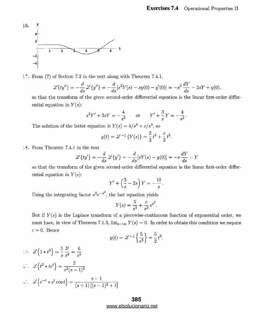
Exercises 7.4 Operational Properties II
!
From (7) of Section 7.2 in the text along with Theorem 7.4.1.
= ~ fs X{y“} = |s2y(s) ~ sy(0) ~ ^ = _ *2 ~ 2sy+!' (0)'
so that the transform of the given sccond-order differential equation is the linear first-order differ
ential equation in Y(s):
s2Y! + 3.sK = - 4 or Y' + - Y = - t .s6 s s°
The solution of the latter equation is Y(s) = 4/s4 + c/s'K so
From Theorem 7.4.1 in the text
{t!/} = “ I x lv '} = ~ l lsY{s) ~ v(0)1 = ~s d~h _ y
so that the transform of the given sccond-order differential equation is the linear first-order differ
ential equation in Y(s):
‘A — 2Using the integrating fa,ctor s e s , the last equation yields
I/-/ x 5 C „2
y (S) - ^3 + ^3 e‘ •
But if Y(s) is the Laplace transform of a piccewise-continuous function of exponential order, we
must have, in view of Theorem 7.1.3, l im ^ ^ Y (,s) = 0. In order to obtain this condition we require
c = 0. Hence
I J C o4 ooS S'*
2\2
<9—1
385www.elsolucionario.net
Exercises 7.4 Operational Properties II
22. ¥\e2t*sm t) = 7--- **- J (s — 2)(s2 + 1)
23. A f* eTd r ) = - ¥ { 6 * } = . 1[Jo J s s(s - 1)24. Z£< [ cos r dr 1 = -i?{cos t} — —— = 9 1[Jo J 6* + 1) 5 + 1
25. * { j V c o e r d r } = \ if {a cco st} = + + 1 = 5(s2++2i + ^
26. i f j f T s m r d r \ = - i?{£sin£} = - ( —j~ T T t ) = 7~o— = T T ~—\2{JO J a 8\ dss2 + l j f l( s2 + 1)“ (s2 + l) 2
27‘ * { £ Te dT} = m * {* } = * ( 7 :T )
28. / sinr cos(t — r) dr| = if{sint}if{cos£} = 2 _|_
29. J f { * j f - n r d r } = (± ^
30. * { * £ „ - * } = - I * { £ r e * * } ( I - ^ 3
32- = j y - d * = ^ -1
3 3 ' 2 ' l { ? ( r r i j } = y _ 1 {iZ£!T ^ i } = i y
34. Using i f -1 i 7— rTj 1 = teai, (8) in the text givesI (s ~ a) J
* ~ l { j ( ^ } = i ‘ Te“T d T = i (ate= —y ( a t e - e + 1).
az
35. (a) The result in (4) in the text is i? " 1{F(s)C?(s)} = / * g, so identify
f W = ( ? f p ) 2 “ d ° ^ = ^ T ¥ -
386www.elsolucionario.net
Exercises 7.4 Operational Properties II
f(t.) = sin kt — kt cos kt and g(t) = 4 cos kt
so
i F (s)G(s)} = f * 9 = * J0 f(r)g (t- r)d t
= 4 (sin kr — kr cos kr) cos k(t — r)dr.
Using a CAS to evaluate the integral we get
Then
c - . r ,8 ^ ;(s2 + A:2)3i f 1 ^ = t sin kt — kt1 cos kt.
(b) Observe from part (a) that
i f {£(sin kt — kt cos kt)} =8 fc3s
(s2 + fc2)3 ’
and from Theorem 7.4.1 that i f {£/(£)} - —F'(s). We saw in (5) in the text that
ifjs in kt — kt cos kt} - 2k3/ (s2 + k2)2,
so, 7 m d 2fc3 8kzs2{t(sm kt - ktcoskt)} = - - .
The Laplace transform of the differential equation is
1~£{y} + y} — f 2 “ i \ +
2s(s2 + 1) (s2 + l)2
Thus
= , . -1 + 2s(s2 + l ) 2 (s2 + l )3
and, using Problem -35 with k = 1,
y = 7r(sint — tcost) -f- -^(tsini — i2cosi).£ "A
The Laplace transform of the given equation is
Solving for if{ /} we obtain if{ /} = -9 7- . Thus, f(t) = sini.
1. The Laplace transform of the given equation is
if{ /} = i f {2 i} — 4 if{s in i} if{ /} .
387www.elsolucionario.net
Exercises 7.4 Operational Properties II
Solving for if{ /} we obtain
.s/f, _ 2s2+ 2 _ 2 1 8 V5J _ ^1! rfl I c\ — c „2 +s2(,s2 + 5) 5 s2 5\/5 52 + 5
Thus2 8
/(£) = -t + 7-7= sin V51.o oVo
39. The Laplace transform of the given equation is
<t{f} = y{te‘} +y{t}i?{/}.Solving for i?{/} we obtain
= 7— T^TTTY = I A + 7 1 1 2(.9 — l)3(<s + 1) 8 s — 1 4 (s — l )2 ' 4 (.9 — l )3
Thus1 + 3 * 1 o t 1 _t
m = + -4tel + - -e-‘
40. The Laplace transform of the given equation is
if{ /} + 2 if{cosi}if{/} = 4if{e"*} + ^{sint}.
Solving for if{ /} we obtain
^ { / } = 4f .+ *+ 5 = J - - + 4- 2(s + l )3 s + 1 (s + l )2 (s + l )3
Thus
f(t) = 4e_* - 7te '1 + 4i2e_<.
41. The Laplace transform of the given equation is
i ? { / } + i f { l } n / } = i f { l } .
Solving for i f {/} we obtain if{ /} = — . Thus, f(t) = e_t.5 + 1
42. The Laplace transform of the given equation is
X { f } = 2{c<xt} + 2{e rt}Z { f} .
Solving for i f {/} we obtain
Thus
j(t) = cost + sini.
1 1
8 7+ 1 '
388www.elsolucionario.net
Exercises 7.4 Operational Properties II
43. The Laplace transform of the given equation is
y{/> = y {1} + y {i} - y {jj J ‘(t - r)3/M * J1 1 8 cr rj.3i <v*c /0 1 1 16- + "2 + o %{f} = - + ~2 + T ’S .9 3 S S S4
Solving for if{ /} we obtain
s2(a + l) 1 1 3 1 1 2 I s„4 i c o „ > o q o ^ /i „2 i /< os4 — 16 8 s + 2 8 s - 2 4 s2 + 4 2 s2 + 4
Thus
f(t) = ^e-2< + ^e2t + i sin2t + ^ cos 21.
44. The Laplace transform of the given equation is
y{(} - 2 y {/> = y {e* - e-‘}y{/> .Solving for i f {/} we obtain
f \ -- - = - —____L ^1U i 2s4 2 s2 12 s4 '
Thus
f(t) = - t- — t*. J w 2 12
45, The Laplace transform of the given equation is
s2{y}-y(0) = i f{ l} - if{s in i} - if{ l} if{y } .
Solving for if{ /} we obtain
y, ( 1 _ s2 - s + 1 _ 1 1 2s
iV) ~ (s2 + l)2 ' “ 2 (s2 + l)2 ‘
Thus
y — sint — ^ tsini.
-6. The Laplace transform of the given equation is
»y(s) - i/(o) + e y w + 9y{i}y{j,} = y{i>.Solving for if{ /} we obtain if{y} = -— • Thus, y = ie~3t.
(s + 3)
389www.elsolucionario.net
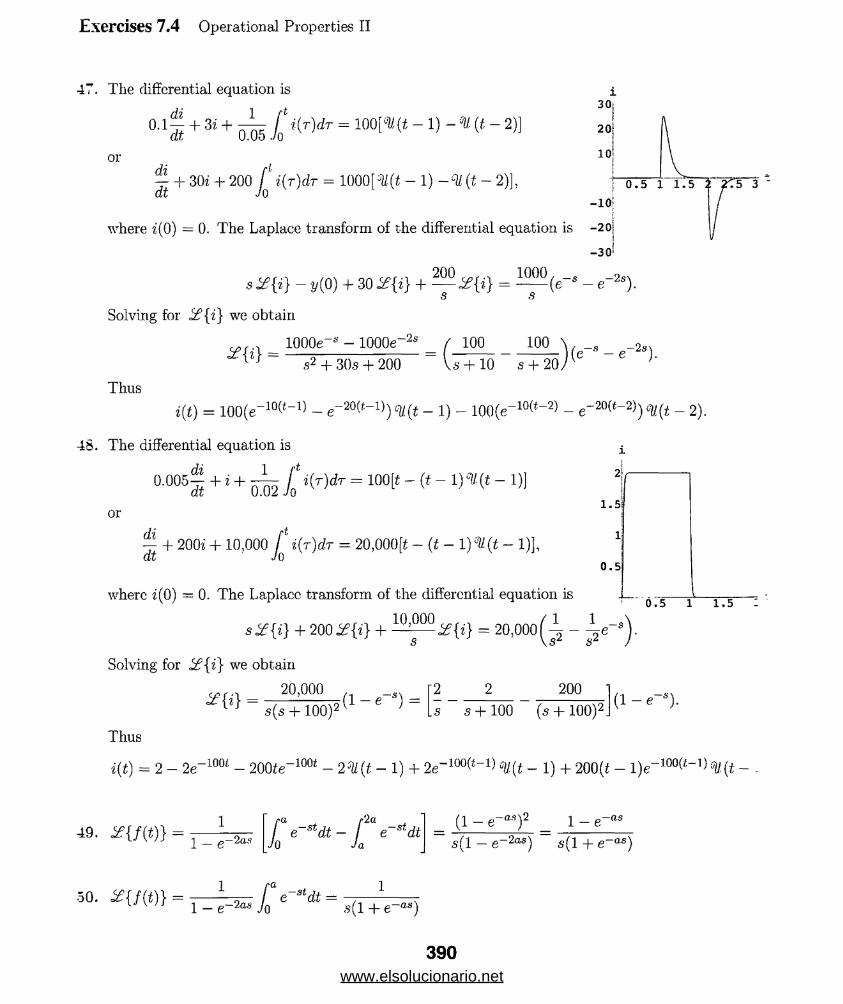
Exercises 7.4 Operational Properties II
47. The differential equation is
di _ 1 f1
or
0.1 + 3i + — jf ' i(r)dr = 100[-K(t - 1) - % (( - 2)]
di— + 30i + 200 / i(r)dr = 1000[^(i - 1) -0/ (t - 2)], dt Jo
20j!
io!
3°|1
; 0 .5 1 1 * 5 ;! 2 7 5 3 -
-10\
where i(0) = 0. The Laplace transform of the differential equation is -20j
-30'
sX{i} - y(0) + 30 2{i} + = ^ ( e ~ s - e~2s).
Solving for ^£{i} we obtain
1000e-s - 1000e~2s*{*} = s2 + 30s + 200
100 100s 10 s -I- 20
(e~s - e~2s).
Thus
i(t) = 100(e_1°^_1) - <r20(t_1)) <m(t - 1) - 100(e_10{*_2) - e~20(t_2)) °V.(t - 2).
48. The differential equation is
,di . 1 /■*0.005^ +i + — J0 ‘(T)dT = 100[t - (t - - 1)]
orrt
— + 200i + 10,000 / %{r)dr = 20,000[* - (t - 1) °U(t - 1)], dt Jo
2
1.5
1
0.5
where z(0) = 0. The Laplacc transform of the differential equation is J— .0 *5 1 1.5
sg{ i} + 200 i?{*} + = 20,0001 1
Solving for Jz?{i} we obtain
200.s s + 100 (s + 100)2J
(1 - c- ).
Thus
■i(t) = 2- 2e~im - 200te~im - 2 sU (t- l)+ 2e-10°(t-1) % t - 1) + 200(i - l)e_100(*~1)5tf(i -
1 - e~2as
/2ci-St u I e-stdt
pa rZ/ e~stdt —
Jo Ja
1 — e—as(1 _ e-^)2
s(l - e_2as) “ s(l + e_as)
50. %{f(t)\ = ---P e~stdt = — — ------- r1 - e~2as Jo .s(l + e~as)
390www.elsolucionario.net
Exercises 7.4 Operational Properties II
Using integration by parts.
* { / « } = T r W o V 1* = J ( s - '
I ' te~"*dt + / ( ' 2 - *)«"’**1 — e—s
,s2(l — e"2s)
. I -st - 7 1 eW2 _|_ e—Jrs/2 2 5TS; ------ / e smtdt — -7y— r • --^ = -s— r coth —
XJ WJ 1 - e-™ 7o s2 + 1 e™/2 - e~ns'2 s2 + 1 2
if {/(£)} = --- s— [ e~stsmtdt = -9 • -— ----u WJ 1 - e '2™ Jo s2 + 1 1 - e ~ * *
The differential equation is L di/dt + Ri = E(t), where i(0) = 0. The Laplace transform
equation is
Ls¥{i}+ RZ{i\ = &{E{t)}.
From Problem 49 we have i f {£(<)} = (1 — e~s)/s( 1 + e~s). Thus
1 - e ~ ' s(Ls + R )X{i} =
-s(l + e"s)
and
1 1 1-c-n = -T
L 5(5 Rf -£')(! 6 s) L s(s "h R/L) 1 + c s
- s G - rrk)(1 - 0(1 - e“+e_2* - ^ +c_4’ - ■ >“ sG - 7Tr/l) ~ 2<r'+2*~2‘ ~ 2c~3“+2e~" - •
therefore.
m = i ( l - e-v/L) - i (1 - e-««-*)/i) %(t - DR y > r+ 1 (1 _ e-*«-2)/i) * (t _ 2) - | ( l - e - « ‘-»)/i) K (i - 3) +
•I o OC= ^ ( l - e~RtfL'\ + 4 V ( - l f ( l - e- ^ t-n)/L) (t - n).
“ n = l
391www.elsolucionario.net

Exercises 7.4 Operational Properties II
The graph of i(t) with L = 1 and R = 1 is shown below.
56. The differential equation is Ldifdt + Ri = E(t), where 'i(O) = 0. The Laplace transform of
equation is
LsZ{i} + R £ { i) = 2{E(t)}.
From Problem -51 we have
1 1 1,.2 $ es — 1
Thus
uid
(.Ls + R )2 { i]1 1 1
s 2 s es _ ]_
L s2{s + R/L) L s(s + R/L ) es - 1
_ W 1 _ 1e — e
Therefore
R\s2 R s R s + R/LJ R\s s + R/L
- -i (l - e-W-‘Z)/L'} % (t _ 2) - ^ ( l - e- ^-3 )/^ % (t _ 3) ---
“ 5 (* ■- 5 ■+ F "R</i) " 5 S (1 - «(*-»>■The graph of i(t) with L = 1 and R = 1 is shown below.
392www.elsolucionario.net
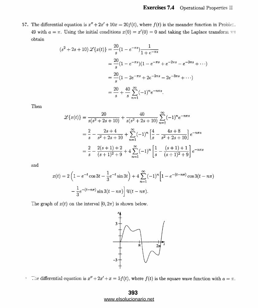
Exercises 7.4 Operational Properties II
57. The differential equation is x" + 2x' + ltte = 20f(t), where f(t) is the meander function in Probl
49 with a — n. Using the initial conditions x(0) = 2/(0) = 0 and taking the Laplace transform
obtainon i
(s2 + 2s + 10) = -^(1 - e— ) _ i - j j
20 .
s
20
s
= — (1 - e-7rs)(l - e~ns + e~27!$ - e-37r's + • • •)
= — (1 - 2e-*B + 2e~2lTS - 2e~Zws + • • •)
20 40 00
T + t E ( - 1 ) Vs s „ in = 1
Then
20+
40 OO
s(s2 + 2s + 10) s(s2 + 2s + 10)
2s+ 4 OC
s s2 + 2s + 10 2 2(s + 1) + 2
n— 1
oc-
4s+ 8
s s2 + 2s + 10.
1 (s + l) + l
s (s + l)2 + 9-rms
and
/ 1 \ 00 rx(t) = 2(1 — e~l cos 31 — sin 3t J + 4 ^ (—l)n 1 — e-(*-rwr) COs 3(t — mr)
' 3 / n=1 L
— sin3(£ — mr) °U,(t — niT).
rhe graph of x(t) on the interval [0,27r) is shown below.
'lie differential equation is x" + 2x' + x = 5f(t), where f(t) is the square wave function with a — ~.
393www.elsolucionario.net
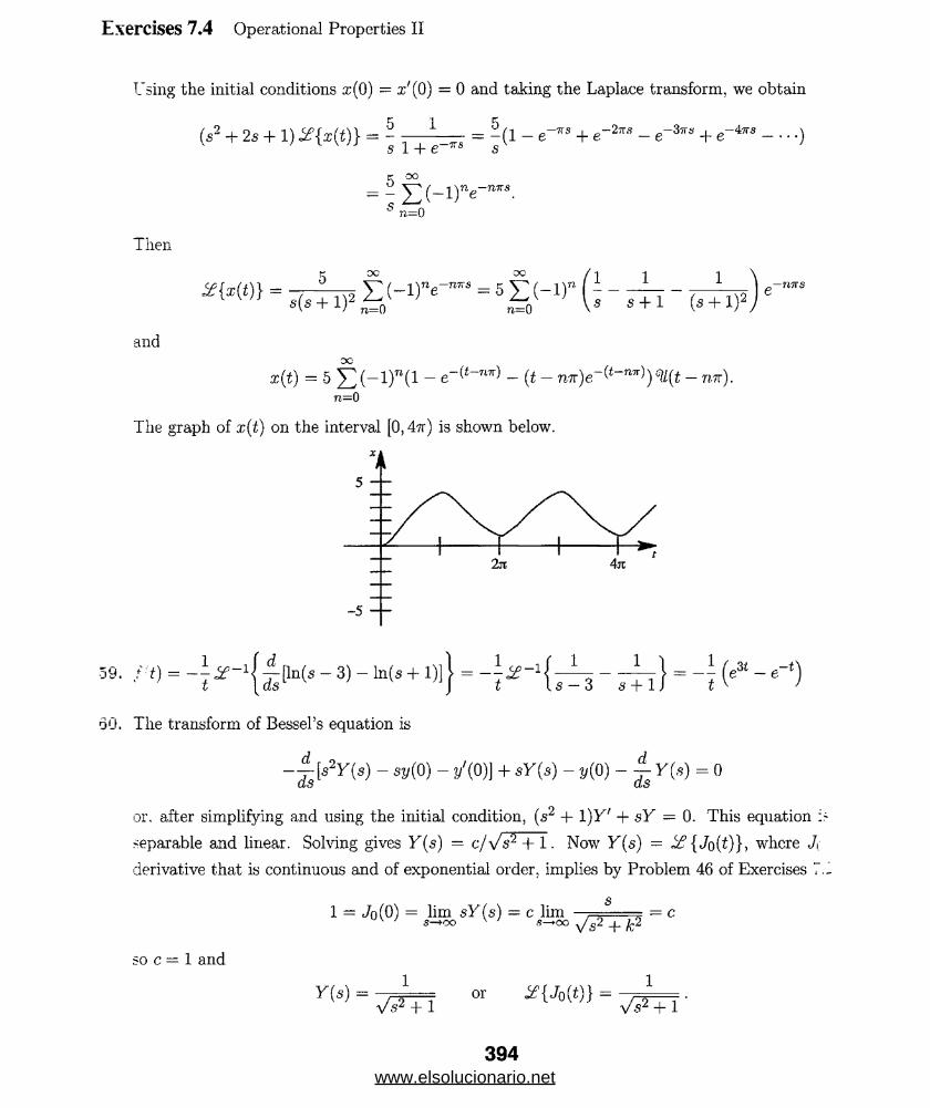
Exercises 7.4 Operational Properties II
Using the initial conditions x(0) — x'(Q) = 0 and taking the Laplace transform, we obtain
(.s2 + 2s +1) y{i(t)} = -s = 5(1 - e-” + e■ITS I —27rs _ 3tt6‘ ~ '7rs
IT -DO- - V ( - l) ne“n™.
S n=0
Then
OC
* ( * » - ^ " 5S (' i r U - JTT - (TTIP.
andC5C
x(t) = 5 £ (- l)n(l - e-^~n^ - { t- n.7r)e-^"n7r)) % t - nn).n=0
The graph of x(t) on the interval [0, An) is shown below.
-riTTS
M- =- H s w - 3) - Ms+1)!} - (e3‘ -*")60. The transform of Bessel’s equation is
- sj/(0) - j/(0)] + sY(s) - j,(0) - 1 Y («) = 0
or. after simplifying and using the initial condition, (s2 + 1)1"' + sY = 0. This equation ir
reparable and linear. Solving gives y(s) — c/x/s1 + 1. Now Y(s) = '<£ { Jo(i)}> where Jr
derivative that is continuous and of exponential order, implies by Problem 46 of Exercises 7.1
1 = Jo(0) = Urn sY(a) = cHm ^ - c
so c = 1 and
Vs2 + 1 Vs2 + 1
394www.elsolucionario.net
Exercises 7.4 Operational Properties II
[s2Y - sy(0) - 1/(0)] + sY - y(0) + ^ [sY - y(0)] + nY
= -4- [»2Y] + sY + — [sY] + nY as as
= - s2( f ) - 2sK+*y + < f ) + y + " y
= ^ (lla) + (1 + n ~ s)y = °-
Separating variables, we find
■51. (a) Using Theorem 7.4.1. the Laplace transform of the differential equation is
dY 1 + n• — s , ( n 1 + n\ , ds = ---------- ds
Y s2 — s ' Vs — 1 s
In Y = nln(s — 1) — (1 + n) In s + c
($ - 1)»Y = c i sl+n
Since the differential equation is homogeneous, any constant multiple of a solution
be a solution, so for convenience we take ci = 1. The following polynomials are sol'.
Laguerre’s differential equation:
n = 0 : Lo(t) = i f -1 j- j = 1
» = l :
- a :
c> 2 o 1 ,= 1 - 4t + 3t? - -13 + — t4.
3 24
(b) Letting fit) = tne t we note that f k\G) = 0 for k = 0, 1, 2, . . . , n — 1 and / ;; =
395www.elsolucionario.net
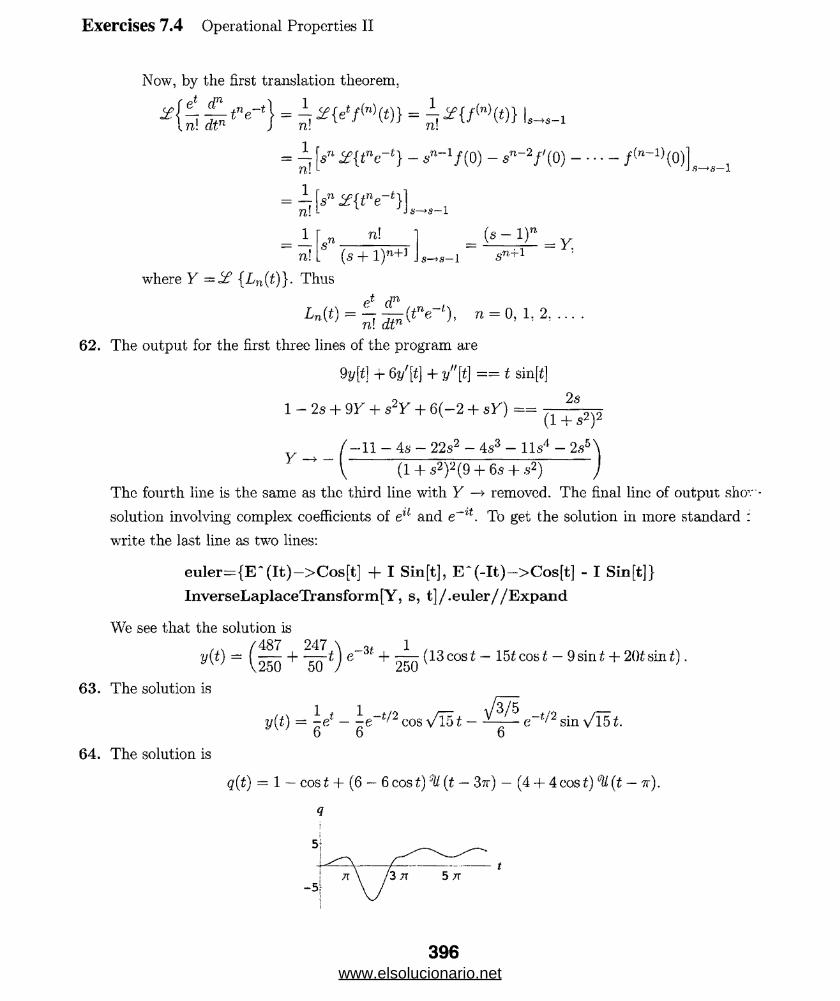
Now, by the first translation theorem.
H ^ tner' } = = l—
- i[ s n y{t"e-*} - »”-'/(0) - s"-2/ '(0 )-----/<’*-1>(0)] i ;; t
^ 1 Ln n! 1 _ (g - *)" ■ yn !L (s + l ) n+J J « - s- i sn+1
where F {Ln(t)}. Thus
= n = 0 ,1 :2 , . . . .
62. The output for the first three lines of the program are
9y[t] + §y'{t] + y"[t] == t sin[£]
1 - 2s + 9Y + s2Y + 6(—2 + sY) - (1 + s2)2
_ / - l l - As - 22s2 - 4s3 - 11s4 - 2s5\
\ (14- s2)2(9 + 6s + s2) JThe fourth line is the same as the third line with Y —> removed. The final line of output shov-
solution involving complex coefficients of eu and e~%t. To get the solution in more standard :
write the last line as two lines:
euler={E', (It)->Cos[t] + I Sin[t], E~(-It)->Cos[t] - I Sin[t]} InverseLaplaceTransform[Y, s, t]/.euler//Expand
We see that the solution is
(487 947 \ 1—— + -^rt) e~3t + — - (13cos£ — 15£cosi - 9sin£ + 20tsin£).2 o 0 5 0 / 25 0
63. The solution is
V(t) = L ‘ - L —‘/2 cos ^ 1 _ V p e-m sin V i51.yw 6 6 6
64. The solution is
q(t) = 1 — cos t + (6 — 6 cos t) ‘JU (t — 37r) — (4 + 4 cos t) (t — tt).
9
Exercises 7.4 Operational Properties II
396www.elsolucionario.net
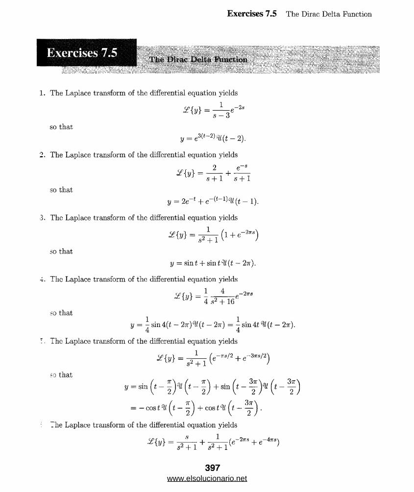
Exercises 7.5 The Dirac Delta Function
Exercises 7.5
1. The Laplace transform of the differential equation yields
i f {y} = —2sS — 3
so thaty = ^ - 2 ) ^ _ 2 )_
2. The Laplace transform of the differential equation yields
, , , , 2 e“s
- i n + i n
so that
y = 2e t + e ^ (t — 1).
3. The Laplace transform of the differential equation yields
^ « = j r n ( 1 + < rW )
so that
y = sini + sin t ,:U(t — 2n).
4. The Laplace transform of the differential equation yields
in = -14 ,s2 + 16
- ‘2ns
so that
y = ^ sin4(t — 2%)°U(t — 2ir) = ^sin4t °U(t — 2-k).
:. The Laplace transform of the differential equation yields
^ “ p s T I («~” /2 + «‘ 3” /2)
so that
v=sin (f “ I)* (‘_ I)+ sin (*- f)* (*_ f)= — cos t % (t — + COS t (t. — ) .
The Laplace transform of the differential equation yields
s 1VY = +
32 + 1 S2 +
397www.elsolucionario.net

Exercises 7.5 The Dirac Delta Function
so that
y = cost + sinif5?/^ — 2 tt) + °U(t — 4?r)].
The Laplace transform of the differential equation yields
=1
so that
s2 + 2.9
1 1
(1 + 0 =ri l i i
y = 2 ~ 2 e~* +
12 s 2 s + 2J
n iit- i) .
(i + O
.2 2
5. The Laplace transform of the differential equation yields
3 1 3 1 1 1%sv\ _ 3 + 1 + -- _-- e~^
m s2(s — 2) s(s — 2)+
n i i n 2s
so that
4 s - 2 4 s 2 s2
°U(t- 2).
2 s — 2 2 s.
L2 2J
9. The Laplace transform of the differential equation yields
1
(s + 2)2 + 1— 2tt s
so that
y ^ e-2 -2vh m tcU(t - 2tt).
10. The Laplace transform of the differential equation yields
2{y} =i
(s + 1)
so that
y = { t- l ) e ~ ^ % { t- l ) .
11. The Laplace transform of the differential equation yields
n y ] = , 4 t ‘. +
e-7TS‘ e-37T5
s2 + 4s + 13 s2 + 4s + 13
3 (s + 2)2 + 32 + (s + 2)2 + 32 ' 3 (s + 2)2 + 32
y = ^e_2t sin31 + e~2t cosSt + ie _2^_7r sin 3(t — tr) JU(t — tt)O o
+ ~e_2(i_37r) ain 3 (t — 3iv)°V*(t — 3tt).o
8 + 2 1+ - (e-™ + e_37r'
so that
s)
398www.elsolucionario.net
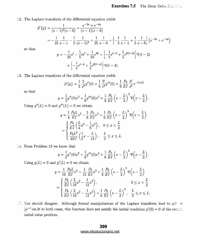
Exercises 7.5 The Dirac Delia r
12. The Laplace transform of the differential equation yields
1+
e~2s + e~4s
(s - 1 )2(s - 6) (s - l)(s - 6)
1 1 1 1^ ~ +
25 s — 1 5 (s — l )2 25 s — 6
1 1 1 1 +
so that
y = e* - -te* + — e6i + y 25 5 25
1
~5e
5 s — 1 5 s — 6.
2)i-2 + I e6(*-2)5
+ --e*-4 + i e6(t" 4). 5 ' '5
°U(t- 4).
13. The Laplace transform of the differential equation yields
so that
V = J iA O )*2 + i»'"(0)x3 + i (x - \) k (x - § ) .
Using y"(L) = 0 and y"'{L) = 0 we obtain
1 * 1 Po 3 . 1 -fb / L\\,( L \
~ l m x + I T A x - V ‘T ’ - j J
Po f L 2 1 3—- —x — -XE l \4 6PoL2 (1 L
-x
0 < x < ~
LL\ L— ), — < x < L. 12/ ' 2 ~ ~I 4E l \2
14. From Problem 13 we know that
V = j / ( o y + i / ' t o ) * 3 + i ^ (s - § ) • » ( * - | ) .
Using y(L) = 0 and ?/(£) = 0 we obtain
16 E l
L o 1— r 3
EJ Vl6‘ 12‘
10 < x < —
2
— ( — x2 - — rr3 ( t.- - ')3 - < x < L. E l V16' 12 / 6 E l V 2) ! 2 “ '
You should disagree. Although formal manipulations of the Laplace transform lead to y[t =
|e_< ain 3t in both cases, this function does not satisfy the initial condition y'(O) = 0 of the sect::::
initial-value problem.
399www.elsolucionario.net
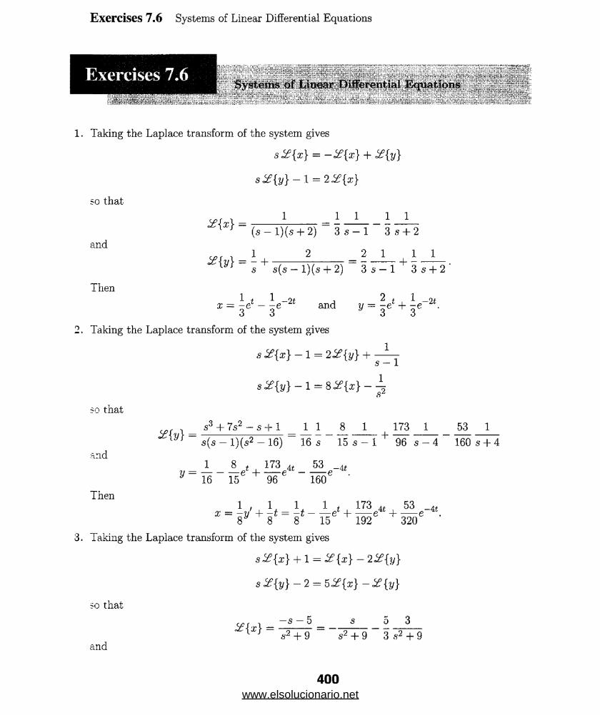
Exercises 7.6 Systems of Linear Differential Equations
Exercises 7.6 *vrr hi >
* ;;''V>'rV r ~ , O :-; ,v *: /;'.;'-";;';r vr- ; rv;r:: rr:r,.;• r : v:Jv“3 rJZxlS. i'l')..'. ; : ~ ?;"';'r ..!'..: 1"**. 'i lIl'X; J17 ?. I V *‘> !*>»«;• ;:r ';L'p:Ii"
1. Taking the Laplace transform of the system gives
s%{x} = -%{x} + 2{y}
sX{y} — 1 = 2X{x}
so that
and
_ 1 _ 1 1 1 1
' X* ~ (s — l)(s + 2) “ 3 s - l ~ 3 7+2
a>f , 1 2 2 1 1 1%{y} = 7 + 1u",-o-v = o — T + o
Then
s 5(5 —l)(s + 2) 3s —1 3s + 2
1 f 1 —Of -, 2 + 1 _Ofa: = -eL — -e and y = -e + -e .
3 3 y 3 3
2. Taking the Laplace transform of the system gives
1s X{x} — 1 = 2 X{y} +
s — 1
s2 {y }- l = SX {x}-\52
so that
f/,f , s3 + 7s2 — s + 1 1 1 8 1 173 1 53 1% { y ) = ,» .2 ^ t - 7; — 7 +
and
Then
s{s - l)(s2 - 16) 16 s 15 s - 1 96 5 - 4 160 s + 4
1 8 f 173 ^ 53 _ 4 fy = -------e ^---- e ----- e .J 16 15 96 160
1 , 1 1 1 t 173 4f 53 _4f
I = 8I , + 8f = 8t - i 5 e' + i « e ' + 320e '•
3. Taking the Laplace transform of the system gives
sX{x} + 1 = X{x} - 2X{y}
s2{y}-2 = 52{x}-X{y}
so that
oj f -> _ s 5 _ s 5 3
W “ ^ T 9 “ “ ? + 9 " 3 ^ + 9and
400www.elsolucionario.net

Exercises 7.6 Systems of Linear Differential Equat
5x = — cos 31—~ sin 3f.
O
Then1 1 7
y = -x — — 2 cos 3t — - sin 31. y 2 2 3
Taking the Laplace transform of the system gives
1(5 + 3) i f {x} + s if {?/} —
s
so that
and
Then
(s - 1) £?{x} + (,s - 1) i? {£,} =
, 56--1 1 1 1 1 4 12{v} = O,/ -- TT2 = - o 7 + o — T + O3s(s - l)2 3 6- 3 s - 1 3 (5 - l)2
1 - 2s 1 1 1 1 1 1
3s(a - l)2 “ 3 s ~ 3 s- 1 “ 3 (s - l)2 ‘
1 1 t t j 1 1 t 4. tx = 3 ~ r ' - 3 t€ and y = ~ 3 + r + 3te -
Taking the Laplace transform of the system gives
1(2s — 2) if{;r;} + sif{y} =
s
so that
ands(s — 2)(s — 3) 2s 2s — 2 s — 3
, 3 s - 1 1 1 5 1 8 1*{»> = = - ; : - s r ^ + ;
Then
s(s — 2)(s — 3) 6s 2 s — 2 3 s - 3'
X = - i + |e2‘ - 2e» and y = - 1- - \e2* + |e3‘ .
Taking the Laplace transform of the system gives
{s + l ) 2 { x } - { * - \ ) 2 { y } = - \s i f {x} + (s + 2) i f {y} = 1
so that
s H- 1/2 s "h 1/2%{v} = s2 + S + 1 (s + 1/2)2 + (v/3/2)2
and
www.elsolucionario.net
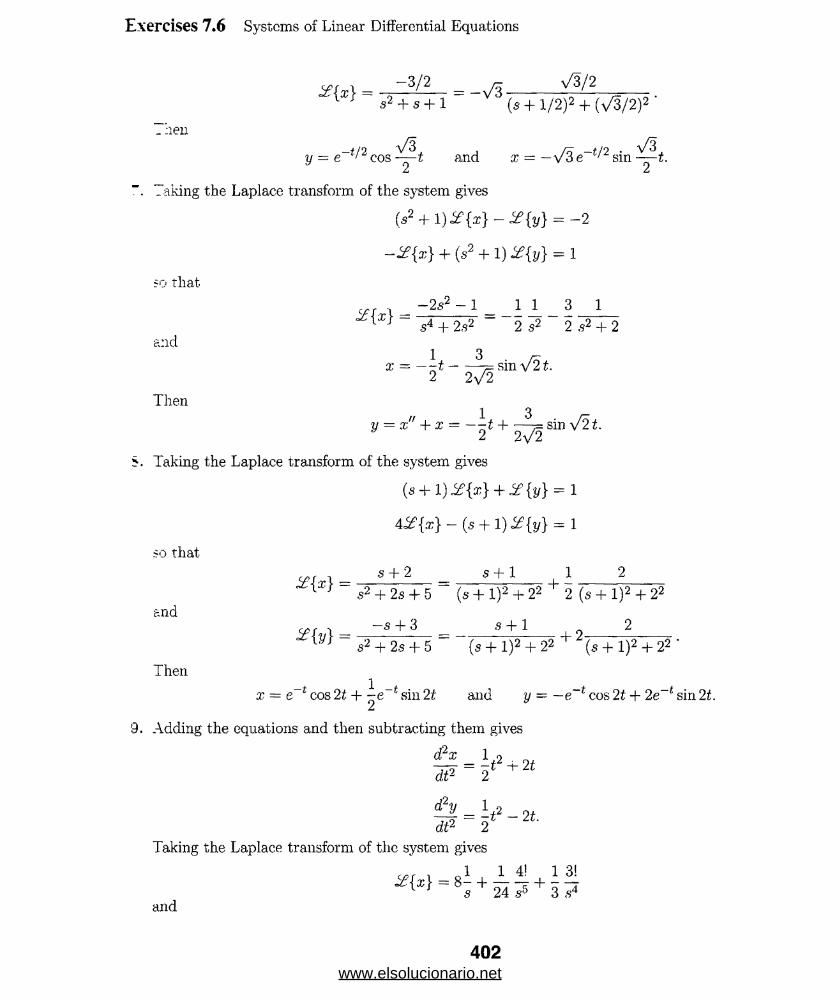
Exercises 7.6 Systems of Linear Differential Equations
2?(x\ : ^ = -y/%_______ \/3/2_______' 1 s2 + s + 1 ‘ (s- + 1/2)2 + (\/3/2)2 '
7:ien
y = e-^ 2 cos and x = —VSe~^2 sin
Taking the Laplace transform of the system gives
(s2 + \)%{x}-!£{y} = -2
+ (s2 + 1) %{y} = X
so that
crr ^ _ -2s2 -1 1 1 3 1
W “ s4 + 2s2 2 s2 2 s2 + 2and
1 3 .
Then// 1 3 . r-
y = x +x = --t + ^-j=smV2t.
?. Taking the Laplace transform of the system gives
(s + l)X{x} + 2{y} = l
4 # { * } - (* + l)2 {y } = l
so that
and
v ? r i _ -s + 2 _ s + 1 1 2
W " s2 + 2s + 5 “ (s + l)2 + 22 2 (s + l)2 + 22
OJ r _ ~s + 3 __ s +1 2‘2 , o„ I e I 1N2 I 02 2-
Then
s2 + 2s + 5 (s + l)2 + 22 (s + l)2 + 22 '
x = e~f cos 21 + ^ e~* sin 2t and y = — e“* cos 2t + 2e-< sin 2i.
9. Adding the equations and then subtracting them gives
d2x 1 o
W = 2t 2‘
^ = i / 2 - 2<dt2 2
Taking the Laplace transform of the system gives
1 1 4 ' 13'
^ > = 8; + 2 4 ? + 3 7 and
402www.elsolucionario.net
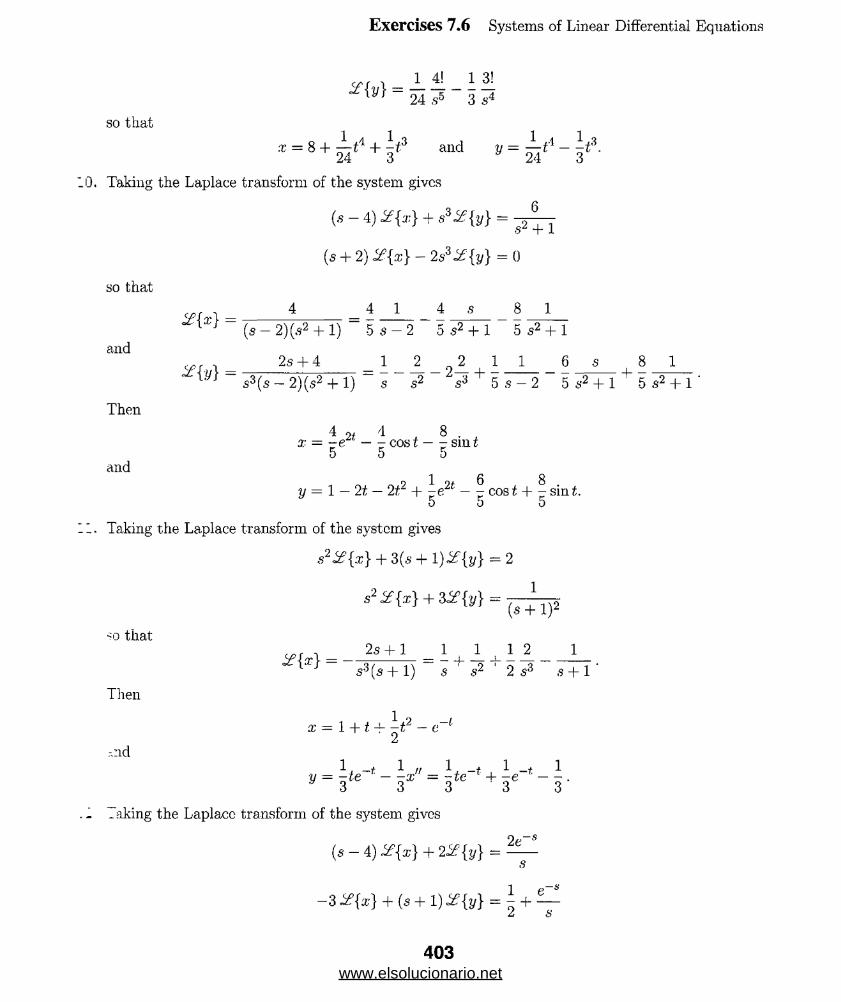
Exercises 7.6 Systems of Linear Differential Equations
1 4f l 31
so thato 1 4 1 1 , 1 4 1 O
I = 8 + 24t ' + 3t ^ V = T4f - f -
10. Taking the Laplace transform of the system gives
(*-4) *{*} + »»:*{!,} = 2^
(s + 2) %{x} - 2s32{y} = 0so that
and
Then
and
so that
Then
:id
*{»} = 4 4 1 4 , 8 1(s-2 )(s2 + l) 5 5 - 2 5 s2 + 1 5 s2 + 1
r 1 2s + 4 1 2 0 2 _ 1 1 6 s* {y} = ^ 7T~on/-9 , ^ = - - - o - 2 z* + cs3(s — 2)(s2 + 1) s s2 s3 5 s —2 5 s2 + 1
4 of A 8 .x — -e — - cos t — - sm t
5 5 5
0 1 w 6 8y = 1 — 2t — 2tr + ye — - cos t + - sin£.
gives
s2i f {.x} + 3(s + {y} = 2
s*2{x} + Z2{y} = 1(s + I f
2s+ 1 1 1 1 2
s3(s + 1) s ' s2 ' 2 s3 s + 1 '
x = 1 + t -f -12 — e 1Zi
1 _f 1 „ 1 _f 1 _f 1
y = 3te ’ ~ r = 3te + 3e - 3
faking the Laplace transform of the system gives
( * - 4 ) * { s } + 2 i f { ! , } = ^
- 3 i? M + (s+ l)if{ !,} = i + ^
403www.elsolucionario.net
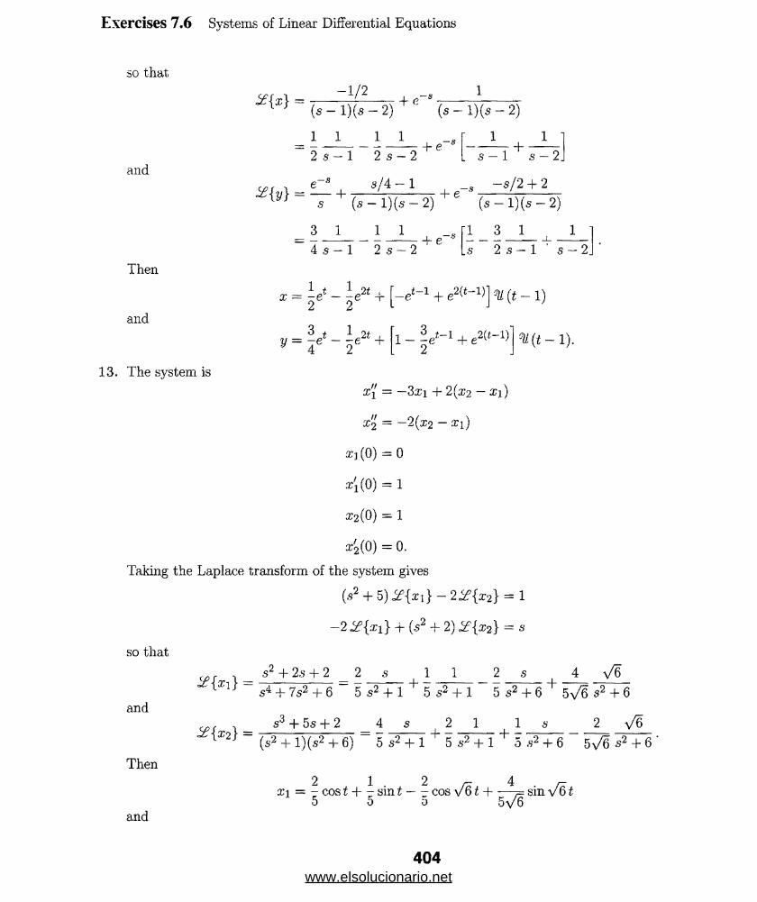
Exercises 7.6 Systems of Linear Differential Equations
so that
1
(s - 1 )(s - 2)
1 1 1 1
(s - l)(s - 2)
and2 s — 1 2 s — 2
<u> r -I e ~ S 5/4 — 1■5%} = — +
+ e~1 1
+
s (s — l)(s — 2)
3 1 1 1
+ e
I s- 1 s - 2
s / 2 + 2
( s- l ) (s-2 )
1 3 1 1
Then
and
s 2 s — 1 ‘ s — 2j '
ar = ie* - + [—e*-1 + e2 1)] ^ (i - 1)
y = je* — ^e2t + [l — ^ (t — 1).4 2 L 2 J
13. The system is
x'l = —3»i + 2 (x2 - xi)
A = -2(x2 - ®i)
zj (0) = 0
•xi (0) = 1
a?2(0) = 1
4 (° ) = 0.
Taking the Laplace transform of the system gives
(s2 + -5) <£{x i}-2X{x2} = 1
—2 + (s2 + 2) if{ » 2} = s
so that
and
Then
and
s2 + 2s + 2 2 s 1 1 2 s 4 v/6} s4 _j_ s2 _|_ g 5 s2 + 1 5 s2 + 1 5 s2 + 6 5\/6 s2 + 6
# { * 2} =2 V6s3 + 5s + 2
(s2 + l)(s2 + 6) 5 s2 + 1 ' 5 s2 + 1 ' 0 s2 4-6 5\/6 s2 + 6
2 1 2 ^ - 4 nxi = - cos i H— sin t -- cos v 61 H--- 7= sin v 61
5 5 5
404www.elsolucionario.net
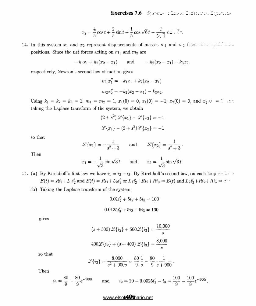
Exercises 7.6 S v;-t:
4 2 1 ,_i —Xo = - cos t + r sin t + - cos y/61---^ •. •;'.
o o 5 5\ o
4. In this system x\ and x2 represent displacements of masses m \ and m* from v.:
positions. Since the net forces acting on mi and m2 are
—kix 1 + k‘2 (x2 — .xi) and — k2 {x2 — ^i) — ksX2 -
respectively, Newton’s second law of motion gives
mix'{ = — k\x\ + k2(x2 ~ %i)
rri2X2 = -k2(x2 — xi) — kzx2.
Using k\ = k>2 = A:a = 1. mi = m2 = 1, 2:1(0) = 0, a’i(0) = — 1, £3(0) = 0. and Xo .O =
taking the Laplace transform of the system, we obtain
(2 + s2) X{xi} - X{x2} = -1
¥ { x } } - ( 2 + s 2) ¥ { x 2} = - 1
so that
“ d = 52^ 3 -
Then
Si = ---p. sin \fz t and x2 = —7= sin VSt.y/3 V3
5. (a) By KirchhofFs first law we have «i = i2 + 1 3 . By Kirchhoff’s second law. on each loop
E(t) = R i] +Lii '2 and E(t) = Rii+L 2 i{] or Lii^+Rh+R-h = E(t) and L2 i -\-Ri2-\-Riz
(b) Taking the Laplace transform of the system
0.01*2 + 5 i2 + 5*3 = 100
0.0125 3 + 5 i2 + 5 i3 = 100
g iv e s
(s + -500) X { i2} + 500i?{i3} =
so that
s
8,000s
8.000 80 1 80 1
400if{i2} + (s + 400) #{*3} =
¥{h} =
Then
s2 + 900s 9 s 9 s + 900
and *, = 2 0 - 0 .0 0 2 5 ^
405www.elsolucionario.net

Exercises 7.6 Systems of Linear Differential Equations
(c) Z;l = i-2 + h = 20 — 20e 9004
16. (a) Taking the Laplace transform of the system
*2 + *3 + 10»2 = 120 - 120 - 2)
—10^2 “1" 5^3 + 0'/-3 — 0
gives
(s + 10) i f {*2} + si?{*3} — —~ ( l — c
-10s^f{*2} + 0(3 + 1) % { ; h } - 0
so that
and
Then
and
120(s +1)
(3s2 + 118 + 10)5
240
48 60 12 + —
3s2 + 11s + 10
3 + 5/3 s + 2 s
240 240
s + 5/3 8 + 2
i2 = 12 + 48e~5t/3 - 60e~2t - [l2 + 48e_5(t_2)/3 - 60e_2(‘_2)] *ll(t - 2)
i3 = 240e~5t/3 - 240e~21 - [240<T5(t~2)/3 - 240e~2(t-2)]cK(t - 2).
(b) h = %2 + «3 = 12 + 288e_5i/3 - 300e“2t - [l2 + 288e_5(*_2)/3 - 300e_2(*~2)l (t - 2)L J
17. Taking the Laplace transform of the system
«2 + 11*2 + 6*3 = 50 sin t
?3 + 6i2 + 6*3 = 50 sin t
50(s + 11) if fe } + 6 i f {23} = 2
S ~ r JL
506 if {i2} + (s + 6 )if{ i3} =
>2 + l
so that
^{*2} =
Then
50s 20 1 375 1 145 s 85 1— — ~ -:—~ + TT7TX -. - _ + TTX — +
(s + 2)(s + 15) 0 2 + 1) 13 8 + 2 1469 8 + 15 113 s2 + 1 113 s2 + 1
and
20 _2, 375 _ l5f 145 85 .
,2 = “ l3 c + T w e " + TT3C0&t+m smt
406www.elsolucionario.net
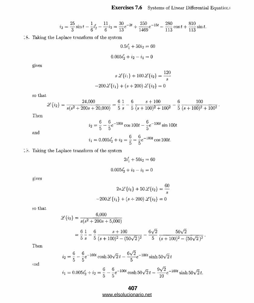
Exercises 7.6 Systems of Linear Differential Equatioi:
25 . 1 . 11. 30 _2t 250 _15f 280 810 .
Taking the Laplace transform of the system
0.5?; + 50?:2 = 60
O.OOS + *2 — *i = 0
gives
sJf{?:1} + ioo^{i2} = —s
-200 { n } + (s + 200) $ {*2} = 0so that
tff 24,000 _ 6 1 6 s + 100 6 100
' ™ “ s(s2 + 200s + 20,000) “ 5 s _ 5 (s + 100)2 + 1002 “ 5 (s + 100)2 + 1002
Then
*2 = 1 - |<rlootcosl00f - ?e-1TOsin lOOt5 5 0
andf' c
i\ = 0.0054 + h = r — -e“ i00< cos lOOt.5 5
Taking the Laplace transform of the system
2 i' + 50*2 = 60
2ives
so that
0.005*2 + *2 -*i = 0
602.s^{ii} + 50i?{z2} = —
- 200# {*1} + (s -!- 200) 2{h} = 0
6,000s(s2 + 200s + 5,000)
6 1 6 s + 100 6\/2 50\/2
Then
.ind
os 5 (s + 100)2 - (50v^ )2 5 (5 + 100)2 - (50\/2 )2
° 6 - I”“ --sh50 5
?‘i = 0.005^ + *2 = r — ^e_100f cosh50\/2i — ^-^e-100* sinh50\/2t. 5 5 10
i ‘2 = -- — -e 10fW cosh 50V21---—-e 100t sinh 50\/2 £5 5 5
www.elsolucionario.net
Exercises 7.6 Systems of Linear Differential Equations
20. (a) Using Kirchhoff’s first law we write ii = %i + 1 3 . Since 1 2 = dq/dt we have i\ — 13 — dq
Using Kirchhoff’s second law and summing the voltage drops across the shorter loop giver
so that
Then
and
E ( t )= iR l + ±q,
h = j r E {t) -JX 1 JrtiL/
dq 1 1
+ #1*3 = E(t)-
Summing the voltage drops across the longer loop gives
E ( t )= n R 1 + L ^ + R 2 h.
Combining this with (1) we obtain
„ r di-3 ^ „ 1 %lR\ + L— + R 2 1 3 = *lR} + ^q
or
l g + J W , - i , = °.
(b) Using L = i?i = R 2 = C = 1, E(t) = 50e~t3il{t - 1) = - 1), ?(°) = *3(0 =
and taking the Laplace transform of the system we obtain
c;np—1(s + 1) * {« } + X {i3} = + -r e ~ ‘
S | -L
(» + 1)^{«3} - ^ { « } = 0,
so that
Jf{g} =(.9+1)2 + 1
and
q(t) = 50e-1e-^~1 si n(t — 1 )°il(t — 1) = 50e“* sin(t — 1 )°U(t — 1).
21. (a) Taking the Laplace transform of the system
40" + $2 + 80i = 0
9" + $ 2 +202 = 0
408www.elsolucionario.net
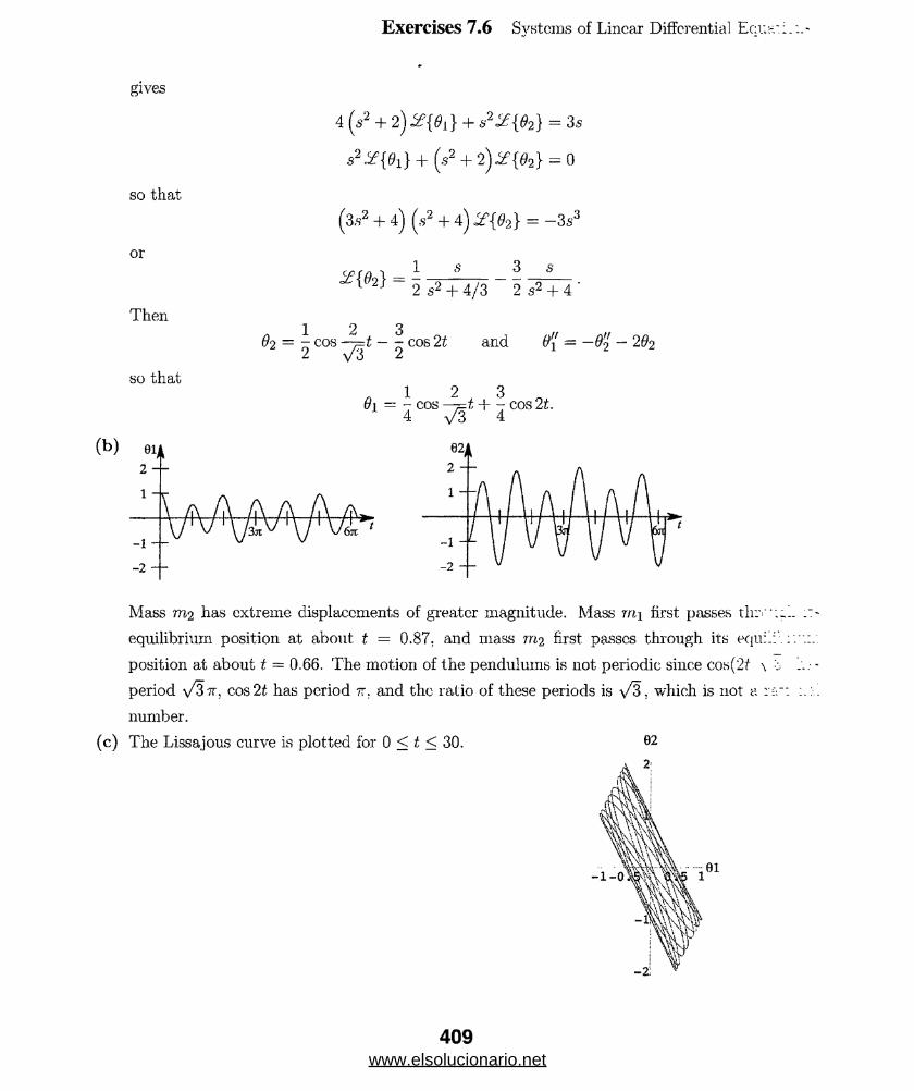
gives
4 (s2 + 2 ) ££{0i} + .52if{02} = 3s
s2X{01}+ (s2 + 2 )# { ^ } = 0
so that
(3s2 + 4 ) (s2 + 4 ) ¥{92} = -3s3
0r
^ } = i ? T 4 7 5 - 5 ? T I '
Then
@■2 = 7: cos ^ cos 21 and 0 '{ = —&'{ - 26*22 y 3 2
so that1 2 3
6\ = - COS — + - cos 21..4 y/ 3 4
Exercises 7.6 Systems of Linear Differential Ecua::.:.-
Mass m2 has extreme displacements of greater magnitude. Mass mi first passes tlr-vul. ;>
equilibrium position at about t = 0.87, and mass m2 first passes through its equ:l:\
position at about t = 0.66. The motion of the pendulums is not periodic since cos(2f \ 0 .. .■ -
period cos 21 has period tt. and the ratio of these periods is \/3, which is not a
number.
(c) The Lissajous curve is plotted for 0 < t < 30.
409www.elsolucionario.net

Exercises 7.6 Systems of Linear Differential Equations
d ) t=='o' ~ t= l /
“ ■ A - " 1
t=2 /
t-5 j
//
t 0i 021 -0 .2111 0.82632 -0*6585 0.6438
3 0 .4830 -1.9145
4 -0.1325 0.1715
5 -0.4111 1.6951
6 0.8327 -0.8662
7 0 .0458 -0.3186
8 -0.9639 0.9452
9 0.3534 -1.2741
10 0.4370 -0.3502
<Tt=9 t=10
!e) Using a CAS to solve 9\(t) = 02(i) we see that = $ 2 (so that the double
pendulum is straight out) when t is about 0.75 seconds.
t=o.
f ) To make a movie of the pendulum it is necessary to locate the mass in the plane as a func
of time. Suppose that the upper arm is attached to the origin and that the equilibrium posi'
lies along the negative y-axis. Then mass mi is at (x, (t),yi(t)) and mass m2 is at (x2(t), yz
where
x\(t) = 1.6sin0i(£) and Vi(t) = — 16cos0i(t)
and
X2 (t) = xi(t) + 16 sin 8 2 (t) and y2(t) = yi(t) — 16 cos 02 (t)-
A reasonable movie can be constructed by letting t range from 0 to 10 in increments c:
seconds.
410www.elsolucionario.net
Chapter 7 in Review
Chapter 7 in Review*'*JS i v /\ :*
- * 'v. ~r„, d'ViTlL::: -................. c.“ '; ; *c /; ; c* Lc; d .A- u ; ‘.....
- i " pv ~if; .T"J: tT~sRTy€zt4
..................... * s‘"s"'.;"'\ S ........... CJ, K!” c: ,w\ '\l„ '
oe«2
3.
4.
i£{/(i)} ~ j te stdt + (2 — t)e stdt =
% {f(t)j = f\ -stdt = - (e~2s - e~As)•/2 6
False; consider f ( t )=
False, since f(t) = (e*)10 = e10i.
True, since lims_>oo F(s) = 1^0 . (See Theorem 7.1.3 in the text.)
False; consider f(t) = 1 and g(t) = 1.
X{e~7t} = 1s + 7
* { * ' " } = ( r h
^{s in2*} = ^ 4
if{e-3‘ sm2i} = (s + 32)2 + 4
i?{£sin2t} = — ds s + 4.
4s
(s2 + 4)2
.2. X{sin2tcU(t — 7r)} = if{sin2(t — Tr)°U-(t — tt)} =
X - 1 = X ~ l 1 ^ 4 1 = I t 5
s2 + 4
6 s6 f 6
i f -1/ __-__— -— 1 = -e*/3‘ 13s — 1J 1 3 s — 1/3 j 3
<£ = -&-(s - 5)3 J 2
= ( -- 1-=— ^ = + -^7= — 1~ r \ = -- U “ v + ^ ( e vI s2 - 5 J \ 2Vo s + VE 2\/5 s - V E j 2^5 2a/5
411www.elsolucionario.net
Chapter 7 in Review
17.
IS.
19.
20.
21 .
22 *
23.
24.
•'I z - J .
26-
27.
25.
29-
10.s + 29} = ^ { (» -5)2 + 22 + I (7 -1)^ + ^ } = c5<c“s2f + F * ™ 2*
^ _1{ ^ e“5S} = (<-5)^(«-5)
I S^ + 7T2 J IS + 7T S2 + 7r2 J
= cos7r(f — l ) Jl/(t — 1) +sin.7r(f — l)'M(t — 1)
Jg-11 1 , , 1 = -L -L ^ -J , nlr/^__r\ = - i-s in ^ ,l L2s2 + n27T2 J L2 7i7T i s2 + (n27r2)/L2 J Lmr" L
exists for s > —5.
X{te“ f(t)} = - ± F (S- 8).
#{ea4/(* - fc) (t - A;)} = e~ks if{fia<t+fc) /(f)} = e~ks(fk £{eaLf(t)} = e-*^-°)F(s - a)
X { / ear/(r) dr| = - if{eaV(t)} = — — , whereas/o $ s
' I { e a‘ j f ( T ) d r ) = x \ [ ‘ { ( t ) , I t \ - F (s ) - F (s a)±s—a S Cl0
/(f) - to)
.'(*) - / ( f ) ^ ( i- f o )
f( f- to )^ ( t- to )
•'!'0 - / ( f )^ ( f - fo) + f(t)°H(t - h)
*Vf) = t - [(i - 1) + 1 ] - 1) + % t - l)- °U (t-4 ) = t - ( t - 1 )°U(t - 1) - %(t - 4)
-f{/(<)}=\- V * -S2 S Z S
-4s
(s - l)2 (s - l)2 s- 1
■' t) — sint°U(t — tt) - sintM{t — 3tt) = -sin(f - 7r)%(t - n) + sin(f - 3Tr)';U(t - 3tt)
4 * m ) - - ( i ^ T T«-’ (s-1) +
■' t) = 2 - 2^(t - 2) + [(f - 2) + 2]-U(f - 2) = 2 + (f - 2)^/(t - 2)
412www.elsolucionario.net

Chapter 7 in Review
* { m = \+ ? e~2'
32. f(t) = t - t°U(t - 1) + (2 - tyu(t - 1) - (2 - ty:U(t - 2 )= t- 2 ( t- 1 )°U(t - 1) + (:t - 2)->( i - 1
* { / « } = ^ - j s - ‘ + ^ _2'
= -- -------- ---p-t*"1) J------- ~-2(s-l)'e'n t ) } ~ (s _ l )2 (,S- l ) 2 e ‘ + (5 - l )2e
33. Taking the Laplace transform of the difibrential equation we obtain
5 1 2 +
(s — l)2 2 (s — I)3
so that
y = + ^ V .Zi
34. Taking the Laplace transform of the differential equation we obtain
1%{y} = (s — I)2 (s2 — 8s + 20)
6 1 1 1 6 s - 4+ tt: ^ — 7--- .xn . +
169 5- 1 13 (s - 1)2 169 (s - 4)2 - 22 338 (s - 4)2 + 22
so that
y = w / + h te‘ - 4 e4‘ 005 2 t+ S ' " sin 2t
I d. Taking the Laplace transform of the given differential equation we obtain
s3 + 6s~ + 1 1 _•>. 2-- ------ -- e -- ;---—r---— e
s2(s + l)(s + -5) 6,2(-9 + 1)(^ r 5) s(s + l)(.s + 5)
_ 6 1 1 J ^ 3 1 13 1~ T * “H ~Z n ~ X
25 s ' 5 s2 2 .9 + 1 50 s + 5
/ 6 1 . 1 1 1 1 1 1 ^ - 2 ,
V 25 s ' 5 ’ .92 + 4 ’ .9 + 1 100 ' s + 5/ 6
2 1 1 1 1 1+ • — r ) e-2*
so that
5 s 2 s + l 10 s + 5
» ‘= ■- I •+ s* ■* k ' - l e_5‘ - - 2) - i (t - 2 m ~ 2)
+ ±e-(t-2)ou(t - 2) - ^ e"5**-2^ - 2).
413www.elsolucionario.net
Chapter 7 in Review
36. Taking the Laplace transform of the differential equation we obtain
vr . s3 + 2 2 + 2s + s2 _s3/ r\ ^si1(s — 5) s (s — 5)
2 1 2 1 1 2 127 1
125 8 25 s2 5 s3 125 s - 5
so that
37 1 12 1 1 2 37 17^ ~o ~ r ~T +
125 s 25 s2 5 s3 125 s - 5.e s
2 2 1 9 127 5ty ~ --------1-- tT H--- e
125 25 5 125 125 25v ' 5V ' 125
ST. Taking the Laplace transform of the integral equation we obtain
c/>r ! 1 1 1 2
i j that
y(t) — 1 + t + -£2.
5*. Taking the Laplace transform of the integral equation we obtain
( ^ { / } )2 = 6 . ^ or X { /} = ±6-±
that f(t) = ±6t.
■5 9. 7r.king the Laplace transform of the system gives
sif-fz} + i f {j/} = —x + 1 si
4 i f {a;} + sif{y} = 2
:hat
vr , s2 — 2s +1 11 1 1 9 1
s(s — 2)(s + 2) 4 s 8 s —2 8 s + 2 '
1 1 of 9 _2/ i / 9 _Of 1 Ofx = -- + -e2t + -e u and y = -x' + 1 = -e 21 - -e2t + 1.
4 o o 4 4
41. T:-I-iing the Laplace transform of the system gives
J X {*} + S { y } = 18-2
2s if{ :r} + s2if{ y } = 18-2
:hat
c/>r i 2 1 1 1 1 1g{*} = 7T. 0 2 = 0 7 - 0 — ^ +8(8 - 2)2 2 s 2 8-2 (a - 2)2
414www.elsolucionario.net
Chapter 7 in Review
—s — 2 3 1 11 3 1+ T
s2(s — 2)2 4 s 2 s2 4 s — 2 (s — 2)2Then
The integral equation is
10* + 2 j ‘ * T ) d T = 2t + 21.
Taking the Laplace transform wc obtain
, 4 2 \ s« = K +
s + 2 9 2 45 9
s3 ' s2J 10s 2 s2(5s + 2) 8 + a* + 5s + 1 s ;
Thus
The differential equation is
i(i) = -9 + 21 + 9e~V5.
i § + 10s + 1009=10- 10‘" (‘ - 5)'
Taking the Laplace transform we obtain
20% {q } =
s(s2 + 20s + 200)( l- e - 5*)
1 1 1 8 + 10 10
10 8 10 (s + 10)2 + 102 10 (s + 10)2 + 102 ( !-
so that
= Yo~Toe m cos 10i I5 R 1W sin m
~ Y6~ cos 10(i - 5) - JLe-'W-s) sin i 0(t _ 5)
Taking the Laplace transform of the given differential equation we obtain
*{y} =
so that
2w0 ( L 4! 1 5 !+ ^ 5 ! e_ ,L/2\+ ci _ 2! +
E IL 148 s5 120 s6 120 s6 2 s3
y -2wo
E IL
where y,f(0) = ci and y"'(0) = C2. Using y"(L) = 0 and y'"{L) = 0 we find
c‘i = wqL2/24EI. C‘i = —wqL/AEI.
Hence
V = T*IVQ
Y2 EIL1 5 L 4 I? 3 I 3 2 1 / L\* ,
- r ' + r ~~2x + t s + 5 r 2 ) ‘® | 1 -
2 9
32 8 + 1/5
— 5).
C2 3!
6 ’ s4
415www.elsolucionario.net
Chapter 7 in Review
44. (a) In this case the boundary conditions are y(0) = y"{0) — 0 and y(7r) = y"{7r) = 0. If we
ci = y'(0) and c2 = y’"{0) then
s4X{y} - s3y(0) - s2y'(0) - sy(0) - y'"(0) + 4£{y} =% {w0/E I}
and
s — I s + 1 \cfiS i ci 25 . c2^{y} = — ■ t t - : + —
2 s4 + 4 4 s4 + 4 8£J \s (s - l)2 + 1 (5 + l)2 + 1 / '
From the table of transforms we get
C\ C‘2 Woy = — (sin x cosh x + cos x sinh x) + — (sin x cosh x — cos x sinh x) + (1 — cos x cosh x
Using y(tt) = 0 and y"(n) = 0 we find
ci4 E I
(1 + cosh 7r) csch TT, c2 =WQ
2 E I(1 + cosli7r) csch 7T.
Hence
V =W q
8EI(1 + cosh tt) csch 7r(sin x cosh x + cos x sinh x)
— -^-(1 + cosh tt ) csch tt (sin x cosh x — cosx sinh®) + 7777(1 — cos x cosh x).oEI AEl
(b) In this case the boundary conditions arc y(0) = y'(0) = 0 and y(?r) = y'(n) = 0. If we
ci = y/;(0) and c2 = y"'(0) then
s4X{y} - s3y(0) - s2y'(0) - sy(0) - y"’{0) + 4£{y] = (£ {S(t - tt/2)}
andc,( 1 Cl 2s c2 4 wo %{y} = TT • ~ ” + -— — t +2 s4 + 4 4 s4 + 4 4 E I s4 + 4
From the table of transforms we get
y = ~ sin x sinh x + — (sin x cosh x — cos x sinh x)2 4
2
+m
4 E Isin [ x — cosh ^ | — cos | x I ) sinh (a:- I ) ] 5# ( z - | )
Using y(ir) = 0 and y'(7r) = 0 we find
ci = C2 =W q COsh j
E I sinli7r
Hence
V - T-=-z — :—— sm x smii x — —— — -—— (sin x cosh x — cos x sinh x) y 2EI sinh7r 4£Isinh7r^ ’
Wq smh £ . Wq cosh % . .V - zrzrz — r-=- sm x smh x — — —: — —^(sn
4E I sinh n
5 ) cosh ( x ~ I ) - 008 (x - 5 ) sinh (* - f ) M x - 1) •wq
4EIsm x
416www.elsolucionario.net
Chapter 7 in Review
45. (a) With 'J1 = g/l and K = k/m the system of differential equations is
+ = -AT(0i-02)
9 i ' + u 2 d 2 = K ( 0 1 - e 2 ) .
Denoting the Laplace transform of 0(t) by 0(s) we have that the Laplace transform of the
system is
(a2 +o;2)0i(s) = -KSi(s) + KG2(s) + s0o
(s2 + u2)92(s) = KQi(s) - A 0 2(s) + # 0-
If we add the two equations, we get
© 1 (s) + 02 (s) = (00 + i>o) 2 f 2Sz + UT
which implies
#i 00 + 02 (0 = (Oo + ip o) cos ut.
This enables us to solve for first, say, B\(t) and then find 02(O from
02(0 = “ 01 (0 + (00 + '00) cosuit.
Now solving
(s2 + ‘J 2 + K)Q\_(s) - A'02(.s) = s0q
- kQi(s) + (s2 + J 1 4- A')02(s) = sijjQ
gives
[(s2 + co2 + K )2 - K 2]©i(,<5) — s{s2 + J 2 + K)Oo + Kstpo.
Factoring the difference of two squares and using partial fractions we get
z _ s(s2 + u2 -+- A)0o + lisipo _ 0o + s 0o — ' o 5
~' /„2 , , I ,.2 ! r,Ts\ — n „2 I , ,2(s2+cj2)(s2+cu2-t2K) 2 s2+ u2 2 s2 + u2 + 2 K ’
so
01 (0 = ~l> cos -f — cos \/uj2 + 2K t.A Zi
Then from 02(O = —0i (i) + (0o + ^’o) coa cot we get
n / ,\ 0o + Vo , 00-^0 / 9 , +02(0 = — ^— cos ----^— cos y w H 2A t.
(b) With the initial conditions 0j(O) = 0o, (0) — 0, 02(O) = 0y, 02(O) = 0 we have
01 (0 = costotf, 02(O = 00 coswt.
Physically this means that both pendulums swing in the same direction as if they were free
since the spring exerts no influence on the motion (0\(t) and 02(i) are free of K).
417www.elsolucionario.net

Chapter 7 in Review
With the initial conditions 0i(O) = 8q. 6*1(0) = 0. 02(0) = ~$0: &'2(0) = 0 we have
6i(t) = $o cos + 2 K t. $2 (t) = —0o cos + 2K t.
Physically this means that both pendulums swing in the opposite directions, stretching
compressing the spring. The amplitude of both displacements is |0o|- Moreover, 0i(t) ~ do r
@2(t) = —0o at precisely the same times. At these times the spring is stretched to its maxim '.
418www.elsolucionario.net

8 Systems of Linear First-Order Differential Equations
fx\ , (4 —7 \2. Let X = I . Then X = X.
\y Vs o j
( x \ / —3 4 —9 \
3. Let X = y . Then X' = 6 - 1 0 X.
WOO1 —
1
f x \ / I - 1 0 ^
4. Let X = y . Then X' = 1 0 2 X
w l - i 0 1,
/.x^ / 1 -1 IN0 ^
!, Let X = y . Then X' - 2 1 -1 x + - tt2 + 0 + 0
U / 1 1 1 1, t2 J V-*J I 2 /
I’ X \ 1 CO 0 ( e f sin 2t N
-I . Let X = y . Then X; = 5 9 0 x + 4e_* cos 21
U J I 0 1 6 / \ -et
>. -j- = 7x -i- 5y — 9z — 8e 2f: ^ = 4x + y + z + 2e5f; — = — 2y + 32 + — 3c 2fat ' dt at
>. = x — y + 2z + e_< — 3t: = 3x — 4y + z + 2e~f + t: ^ = —2,t + 5y + 62 + 2e~* — t at dt dt
’ . ^ = 3x — 7ty + 4sint + (t — 4)e4*; ^ = :r + y + 8 sin£+ (2t + l)e4t
419
www.elsolucionario.net

Exercises 8.1 Preliminary Theory—Linear Systems
11. Since
X ' = - t o 5t and : : ; > - o -51
we see that
X ' = C - r ) X -
12. Since/ 5 cos t — 5 sin t \ ,
X ' = e and\ 2 cos t — 4 sin t J
—2 5\ / 5 cost — 5sini\ ,
' x - 1 r-2 4 \ 2 cos t — 4 sin £ y
we see that
13. Since
D x -
X ' = ( 3_/2W and ( - 1
we see that
M ' i 1 - i4) x '
14. Since
X' = e* + ( te1 and2 ) X = i - 1 0 / V-l
5\ t ( 4 e‘ +
-4
we see that
x ' = (- i15. Since
X ' =
/OX
0
U /
1
and
1\
6 - 1 0
V-l -2 - i ;
x =/0\
0
\o/we see that
1
X ' =
1 \
6 - 1 0
V-l -2 -1/
X.
16. Since
X' =
/ cos t
^ sin t — 5 cos t
— cos t — sin t /
and
1 0 1\
1 1 0
[-2 0 -l)
X =
/ cos t
^ sin t — cos i
V — cos i — sin t J
we see that
X ' =
i o n 1 1 0
V—2 0 - I J
X.
420www.elsolucionario.net

Exercises 8.1 Preliminary Theory—Linear Systems
17. Yes, since W (X i ,X 2) = —2e ^ 0 the set X i , X 2 is linearly independent on —00 < t < oc.
IS. Yes, since IF(X i, X 2) = Se2t 7 0 the set X i, X 2 is linearly independent on — oc < t < oc.
19. No, since I4''(X i, X 2, X 3) = 0 the set X i , X 2, X 3 is linearly dependent on —00 < t < 00.
10. Yes, since VF(Xi,X2,X;3) = —84e~* ^ 0 the set X i, X 2, X 3 is linearly independent or.
—00 < t < 00.
21. Since
we see that
^ = ( 3 2 l Xp +t +
22. Since
we see that
and1 -1
x K i - i h +
13. Since
X i = e* +
we see that
te and'2 1'
3 4et =
^ = ( 3 ef'.
el +-1
teS
14. Since
* ; =
3 cos St \
0
—3 sin ‘it J
we see that
and1 2 3\
-4 2 0
\—6 1 0/
X.D +
/ —1\
4
3 /
sin St =
1 2 3\
-4 2 0
—6 1 0 /
X« +(~1\
4
V 3 /
sin St.
3 cos St \
0
—3 sin St J
■:. Let
X i =
6 \
-1
V-5/
X 2 =
/ —3\
1
1 /
„ -2 t X , =
/ 2 \
1
VI/
‘it. and A =
/ 0 6 0 \ 1 0 1
V1 1 0 y
421www.elsolucionario.net

Exercises 8.1 Preliminary Theory—Linear Systems
Then
xi =
X '2 =
x; =
/-6\
i
5 /
6 \
- 2 1-2 /
/ 6 \
e~l = A X i,
e~2t = A X 2,
3
V 3 /e3t = A X 3,
and Wr(X i ,X 2, X 3) = 20 ^ 0 so that X i, X 2, and X 3 form a fundamental set for X ' = AX
—oc < t < 00.
26. Let
■fit
and
Then
-yftl
iv +r-nt+/i0
A =
4 j
-1 -1'
o r
X i = [ . ^ i e' V2 '
- 2 - A
' -V2 '
, _ 2 + \/2,
v/5t = A X 1;
- \ /2 1 _= a x 2;
1 ) - A X . + ( i j ! l +
and W (X i,X 2) = 2V2 ^ 0 so that X P is a particular solution and X i and X 2 form a fundair.-
set on —oc < t < 00.
422www.elsolucionario.net
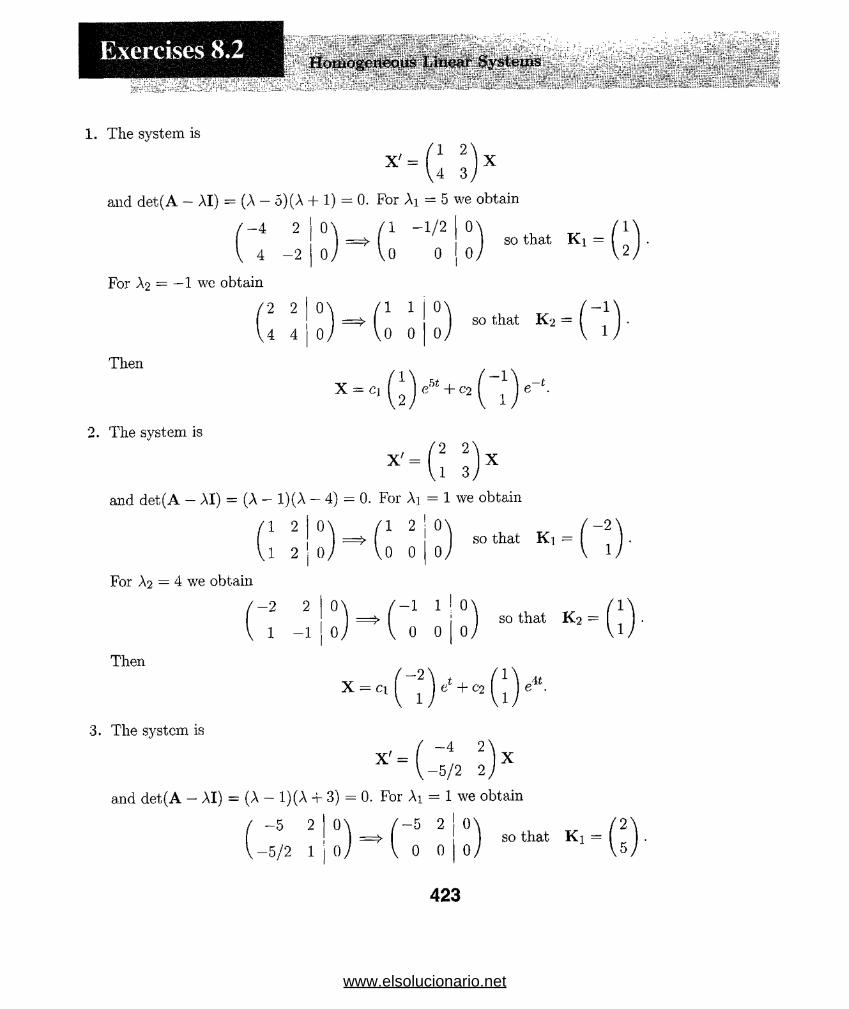
. ' {....... CV ;-" / \ * .•• •• - :••' .....:'w - : «* / . / -Exercises 8.2
1. The system is
x,=C l ) x
and det(A — AI) = (A — 5) (A + 1) = 0. For Ai — 5 we obtain
/ —4 2
V 4 -2
For A2 = — 1 we obtain
/ 2 2
\4 4
Then
2. The system is
O'
0.
0^
0 J
'1 —1/2
,0 0
'1 1
,0 0
so that K i
so that K -2 =
* - ( ! >
and det(A - AI) = (A - 1)(A - 4) = 0. For A] = 1 we obtain
For A2 = 4 we obtain
Then
'1 2
,1 2 j 0,
-2 2
1 -1
'1 2
,0 0 0.so that Ki =
O'
0.
-1 1 ! 0
0 0 0so that K 2 =
1
3. The system is
X = ct | i )<?+c2 r )eit .
X' = ( - " i l ) X
and det(A - AI) = (A - 1)(A + 3) = 0. For Ai = 1 we obtain
-5 2
-5 /2 1 j 0 .
'-5 2
. 0 0 0so that K i
423
www.elsolucionario.net
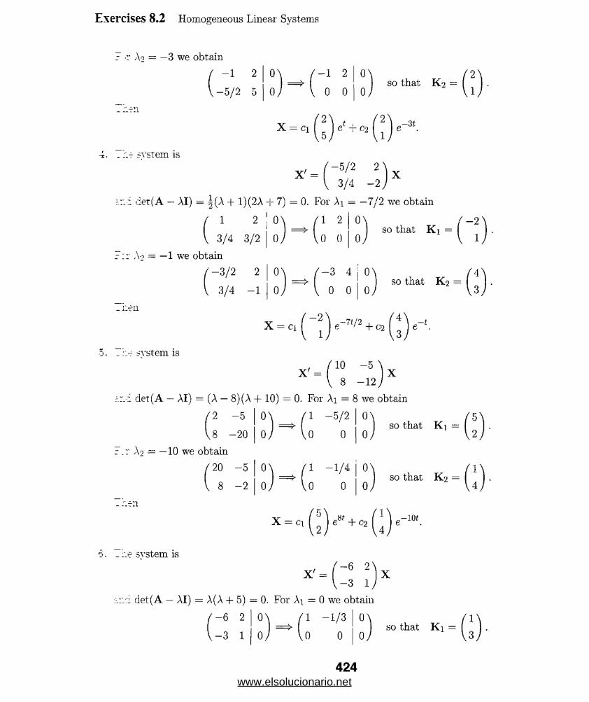
Exercises 8.2 Homogeneous Linear Systems
Ao = —3 we obtain
f " 1 2 V —5/2 5
O'
0.
- 1 2 0 0
so that K 2
system is
X ' = ( 5/2 2 ~) X V 3/4 —2/
iet(A — AI) = ^(A 4- 1)(2A 4- 7) = 0. For Ai = —7/2 we obtain
/ I 2 ! O'
V 3/4 3/2 | 0,
Ao = — 1 we obtain
'1 2
0 0
O'
0,
-3/2 2
3/4 -1
-3 4 0
0 0
so that K i =
so that K 2
rll
system is
+ C2 I I e-t
x ' - ( “ - 12) x
'.:;i det(A — AI) = (A — 8) (A 4-10) = 0. For Ai = 8 we obtain
/ 2 -5
V8 -20
A? = —10 we obtain
20 -5
8 -2
O'
0,
0 ’
0 .
'1 -5/2
-0 0
'1 -1/4
,0 0
0,
O'
0 ,
so that Ki
so that K 2
X = C lQ ) e * + c2 Q ) < r “ ‘.
_ :.e svstem is
X '= ( - 3 l ) X
det(A — AI) = A(A 4- 5) = 0. For Aj — 0 we obtain
-6 2
-3 1
1 -1/3
.0 0so that K i
424www.elsolucionario.net

Exercises 8.2 Homogeneous Linear Systems
For = — 5 we obtain
- 1 2
-3 6
O'
0.
1 - 2
0 0|0 .so that K 2 =
Then
The system is
x = c , ( M + c2 P , e — 5t
/ l 1 -1\
X' = X0 2 0
V0 1 - 1/
and det(A — AI) = (A — 1)(2 — A)(A + 1) = 0. For Ai = 1, A2 = 2. and A3 = —1 we obtain
Ki =
/ 1\ /2\ / 1 \
0 , k 2 = 3 , and K 3 = 0
W U U /
so that
X = ci
/1\
0
\o)
eL + c-2
/ 2\
3
V I/
e2t + C3
/1\
0
V2/
i. The system is2 -7 0\
X' = X5 10 4
Vo 5 2 /
and det(A - AI) = (2 - A) (A - 5)(A - 7) = 0. For At = 2. A2 = 5. and A3 = 7 we obtain
/ 4\ —7\ / —7\
K, = 0 , k 2 =
V-5/
and K 3 —
-o that
X = ci
4\
0
V-5/
5 /
/ —7\
5 /
e2t + C2
—7 \
5
W
"Ae have det(A — AI) = —(A + 1)(A — 3)(A + 2) = 0. For Ai = —1. A2 = 3, and A3 = —2 we obt
/ —1 \ /1 \ / 1\
Ki = k 2 = 4
V3/
and K 3 = -1
3 /
425www.elsolucionario.net

Exercises 8.2 Homogeneous Linear Systems
so that( - 1\
0
1 /
e 1 + C2
/1 \
4
W
e3t + c3
1 \
-1
3 /
2i
10. We have det(A — AI) = —A(A — 1)(A — 2) = 0. For Ai = 0, A2 = 1, and A3 = 2 we obtain
/ 1\ /0\ /1\
K i = 0v-i; k 2 =
so that
X = ci
n
0
v - i /
1
Vo/
/o\
1
U J
, and K 3 = 0
V I/
e1 + C3/1 \
0
w
„2t
We have det(A
~e obtain
AI) = -(A + 1)(A + 1/ 2)(A + 3/2) = 0. For Ai = -1, A2 = - 1/ 2, and A3 = -
K] =
X = ci
( 4 \/-12\
0 IIOl 6
1- 1/ s j
4 N f —12\
0 e_t + c2 6
V-l> V 5J
, and K 3 -
4 \
2
V-i /
e t/2 + c3
4 \
2
v - i /
■-‘■it/ 2
have det(A — AI) = (A — 3) (A + o)(6 — A) = 0. For Ai = 3, A2 = —5, and A3 = 6 we obtr.i
/1\ / 1 \ 2\
K i = 1
Vo/
-1
0 /
, and K 3 2
V11 /
50 that
X = ci
m
1
vo/eM + c2 -1
0 /
+ C3
2 \
- 2V 11 /
Jyt
.3. We have det(A — AI) = (A + 1/2) (A — 1/2) = 0. For Ai = —1/2 and A2 = 1/2 we obtain
K l = ( “ ) and K 2 = Q V
50 that
x=fil ( i ) e' ,/2+C2( i ) et/2-
426www.elsolucionario.net
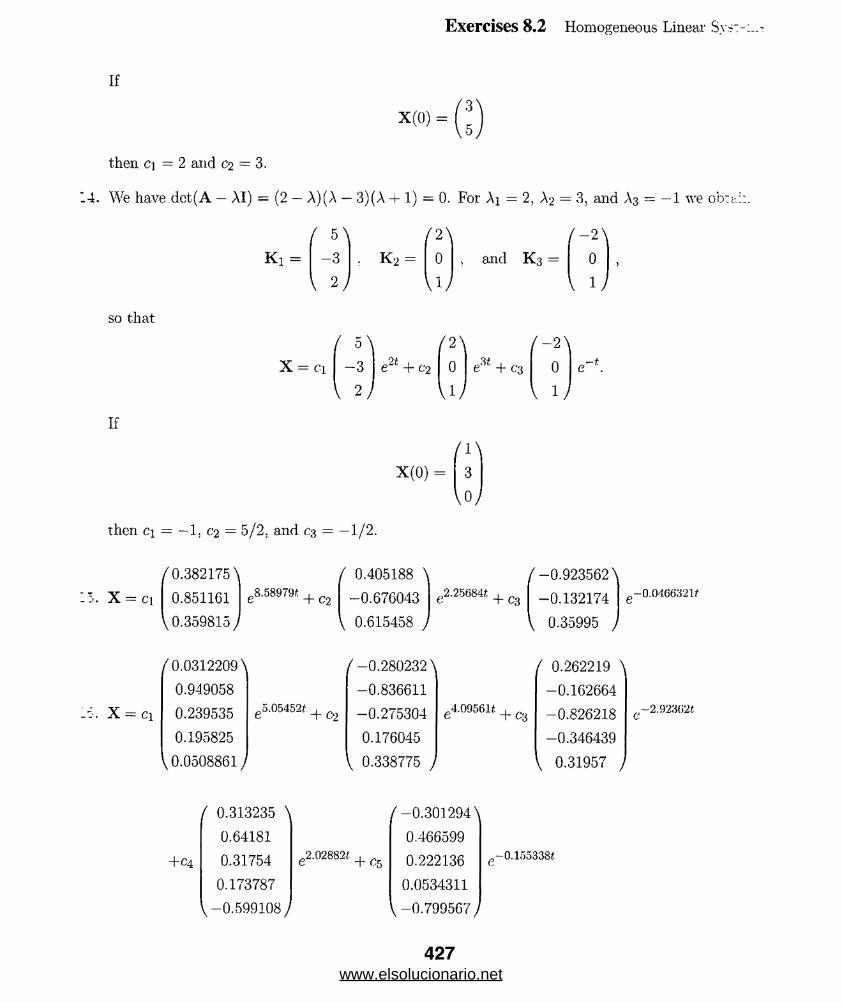
Exercises 8.2 Homogeneous Linear Sy:
If
X(0) ='3'
then ci = 2 and c2 = 3.
'A. We have det(A — AI) = (2 — A) (A — 3) (A 4-1) = 0. For Ai = 2, A2 = 3, and A3 -1 we ob:
5 \ 2\ / —2\
Ki = -3 : K2 = 0 B w CO 11 0
I 2J [ l j W
so that
X = ci
5 \
-3
2 /
e2* + c2
/2\
0
W
eM + cs
/ —2 \ 0
1 /
If
X (0) =
/i\
3
w
then ci = —I, C2 = 5/2, and C3 = —1/2.
X = ci
/ 0.382175 \
0.851161
0.359815/
e8.58979t + C20.405188 \
-0.676043
V 0.615458 /
e2-25684* + C3/-0.923562^
-0.132174
V 0.35995 /
-0.(M66321f
X = Ci
0.0312209 \
0.949058
0.239535
0.195825
V 0.0508861 /
-0.280232 \
-0.836611
-0.275304
0.176045
0.338775 /
.4.095614 , „ e + 6*3
0.262219 \
-0.162664
-0.826218
-0.346439
0.31957 /
-2.923fi2t
+C4
0.313235 \
0.64181
0.31754
0.173787
V-0.599108/
-0.301294 \
0.466599
0.222136
0.0534311
-0.799567 /
e—0.1o5338£
427www.elsolucionario.net

Exercises 8.2 Homogeneous Linear Systems
/ \/ / /f / /
! / // /
(b) Letting ci = 1 and. Ci = 0 we get x = 5e8i, j/ = 2e8*. Eliminating the parameter we ~
y = x > 0. When c\ = —1 and ci — 0 we find y = x < 0. Letting cj = 0 and C2 = '
get x = e-10t, y = 4e-10<. Eliminating the parameter we find y = 4x, x > 0. Letting ci =
and C2 = —1 we find y — Ax, x < 0.
(c) The eigenvectors K i = (5,2) and K 2 = (1,4) are shown in the figure in part (a).
18. In Problem 2, letting c\ — 1 and C2 — 0 we get x = —2et,
y — el. Eliminating the parameter we find y = — x, x < 0.
When ci — —1 and — 0 we find y = —%x, x > 0. Letting
ci — 0 and C2 = 1 we get x = e4*, y = e4t. Eliminating the
parameter we find y = x, x > 0. When ci = 0 and C2 = — 1 we
find y = x, x < 0.
In Problem 4, letting ci = 1 and C2 = 0 we get x — —2e~7t/2,
y = e-7</2. Eliminating the parameter we find y — — x, x < 0.
When ci = — 1 and C2 = 0 we find y = —^x, x > 0. Letting
Cl = 0 and C2 = 1 we get x = 4e~l , y = 3e_*. Eliminating the
parameter we find y = x > 0. When ci = 0 and C2 = — 1 we
find y — ^x. x < 0.
19. We have det(A — AI) = A2 = 0. For Ai = 0 we obtain
A solution of (A — AiI)P = K is
X N
^ ^\
\/ \
428www.elsolucionario.net
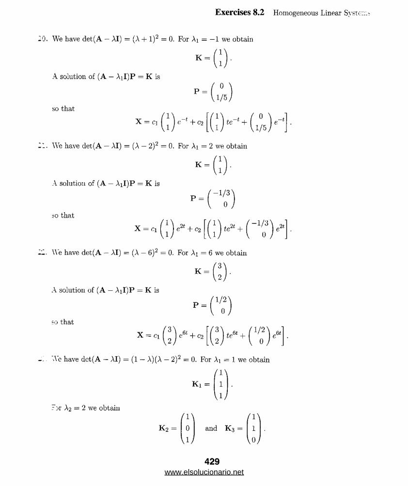
Exercises 8.2 Homogeneous Linear Syst
We have det(A — AI) = (A + 1 )“ = 0. For Ai = — 1 we obtain
A solution of (A — AiI)P = K is
K =
P =
\lj
0 ’
. 1 / 5.so that
X = c, I 1 I <;-'+«1 , 1 / 5 ,
We have det(A — AI) = (A — 2)2 = 0. For Ai = 2 we obtain
1\K =
A solution of (A — AiI)P = K is
P =
,1 / ’
-1/3'
so that
X = c i( i 1 e2* + c21
te2t +-1/3'
We have det(A — AI) = (A — 6)2 = 0. For Ai = 6 we obtain
3\
A solution of (A — AiI)P = K is
K =
P =
so that
x = c i U r +C2
\2J
1/ 2 '
Ac have dct(A — AI) = (1 — A)(A — 2)“ = 0. For Ai = 1 we obtain
/1\
Ki =
':>r A2 = 2 we obtain
\i/
fl\ / 1 \
k 2 = 0 and K 3 = 1
\1) \o)
429www.elsolucionario.net
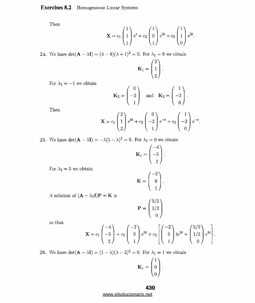
Exercises 8.2 Homogeneous Linear Systems
Then
X = Cl
/1 \
1
V i/
e + C2
/ 1\
0
V i/
e2t + c3
/1\
1
U /
e2i.
24. We have det(A — AI) = (A — 8) (A + l )2 = 0. For Ai = 8 we obtain
K i =
/2\
1
V2 /
For A2 = — 1 we obtain
K 2 =
Then
X = d
/2\
1
w
0\
-2 1 /
e8* + C2
and K 3 =
1\
- 20 /
°\
- 21 /
1\
-2 0 /
25. We have det(A — AI) = — A(5 — A)2 = 0. For Ai = 0 we obtain
Ki =
For A2 = 5 wc obtain
K =
A solution of (A — A2I)P = K is
P =
/ —4\
-5
2 /
/ —2\
0 .
1 /
5/2 \
1/2
0 /
so that/ —4\ / —2\ / —2\ / 5/2\
X = ci -5 + c2 0 e5t + C3 0 teu + 1/2 e5*
I l ) V l j o j
26. We have det(A — AI) = (1 — A)(A — 2)2 = 0. For Ai = 1 we obtain
/1 \
K i = 0
Vo/
430www.elsolucionario.net

Exercises 8.2 Homogeneous Linear Systems
For A2 = 2 we obtain
K =
A solution of (A — AaI)P = K is
P =
0\
-1
1 /
0\
-1
0 /
so thatm
(0\ 0\
X = ci 0 e* C2 -1 e2t + C3 -1 te2t + -1 e2t
U J 1 J I i j I o j
1". We have det(A — AI) = — (A — l)3 = 0. For Ai = 1 we obtain
W
Solutions of (A — AiI)P = K and (A — AiI)Q = P are
/ 0 \ 1/2 \P = 1
Vo /
and Q _ 0
0 /
so that
/0\ /0\ /0\ (0\t2 1 2 C +
/()\ ( W )
X = ci 1 el + C2 1 1 e* + C3 1 1 t(3 -\- 0 e*
U j U J U J U JLi
U J I o j
1* We have det(A — AI) = (A — 4)3 = 0. For Ai = 4 we obtain
/1\
K = 0
V O /ii jlutions of (A — AiI)P = K and (A — AiI)Q = P are
/0\
P - I
Vo/
and Q =
/0\
0
VI/that
m m /OX (1\ j.2 /0\ /0\
X = ci 0 e4t + C2 0 t.eu + 1 e4i + C3 0t Af
2 6 +1 teu + 0 e4t
U J U J U J U JZi
U J U J
431www.elsolucionario.net
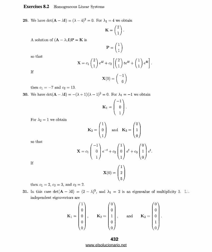
Exercises 8.2 Homogeneous Linear Systems
29. We have det(A — AI) = (A — 4)2 = 0. For Ai = 4 we obtain
'2\
A solution of (A — AiI)P = K is
K =
P =
so that
If
X = ci( ; |e4* + c2
X(0) =
1/
'V-
'2te4t + A t
-1'
then ci = —7 and C2 = 13.
30. We have det(A — AI) = —(A + 1)(A — l)2 — 0. For Ai = —1 we obtain
/-1\
K, = 0
1
For A2 = 1 we obtain
K 2 = and K 3
/ U \
1
VO/
so that
X = C1
/-1 \
0
1 /
+ c2
If
X(0)
/ ! \
0
/i\
2
VW
el + c3
/0\
1
V o /e*.
then ci = 2. c2 = 3, and C3 = 2.
31. In this case det(A ~ AI) = (2 — A)5, and Ai = 2 is an eigenvalue of multiplicity 0. L::.
independent eigenvectors are
Ki =
/ 1 \ 0\ /ON
0 0 0
0 k 2 = 1 , and K 3 = 0
0 0 1
W w
432www.elsolucionario.net

Exercises 8.2 Homogeneous Linear System;
In Problem 20 letting c\ = 1 and c2 — 0 we got x = ef\ y = e*. Eliminating the parameter we fh
y = x, x > 0. When c\ = — 1 and c,2 = 0 we find y = x, x < 0.
In Problem 21 letting ci = 1 and co - 0 we get x = e2t, y = e2t. Eliminating the parameter we fz:
y = x. x > 0. When c\ = — 1 and c2 = 0 we find y = x, x < 0.
// /
y / 1/ / / / / /
/ / / / / / / / //■ / // .c.. r .
/ / / / / / ; / / / / / ■
y / / s // *7 / ■r v
\ \ \
N >s
\
Phase portrait for Problem 20
f t .
... .. ...........--
/ / // / ^V/ i > o / / .
I V */
//
/ /
/ 7 /
. / / /
V // /Phase portrait for Problem 21
Problems 33-46 the form of the answer will vary according to the choice of eigenvector. For exam:.
Problem 33, if K[ is chosen to be ( _ . ] the solution has the form2 - i J
cos t sin tX — Ci I e'u + c2 \e
V 2 cos t + sin t j V 2 sin t — cos t
it
Wc have det(A - AI) = A2 - 8A + 17 = 0. For Ai = 4 + i we obtain
so that
X i = f 2 + * ) e(4+i = ( 2 €OS * ~~ Sln e4t^ i ( co*t + 2 sin f e4t
Then
X = ci
5 cos t J 5sint
2 cos t — sin t \ A4 { cos t + 2 sin teu + C2
5 cos t
We have det(A — AI) = A2 + 1 = 0. For Ai = i we obtain
. V 1)x1=('“1“i)e-'=fsillt"cos‘) +,:
\ 2 I V 2cos( I
r-o that
j L “I- & o,
\ 5 sin teAt.
Ki =
— cos t — sin t '
2 sin t
433www.elsolucionario.net

Exercises 8,2 Homogeneous Linear Systems
Then/sin t — cos t\ ( — cos t — sint '
X = C , l 2 cos? J + H 2 sin t
35. We have det(A — AI) = Az — 8A + 17 = 0. For Ai = 4 + % we obtain
V 2 /
so that
Then
X, = I ' 1 e<4+i>! = ( ‘5in1 ~ m ''‘ ') e11 + i ( - Si" ‘ - 008 ‘ ' \ 2 J \ 2 cost J \ 2 sin t
( sin t — cos t \ ( — sin t — cos t \ MX = c, , I e*° + C2 „ . e4\
\ 2 cos t / \ 2 suit /
e4*.
36. We have det(A — AI) = A2 — 10A 34 = 0. For Ai = 5 + 3i we obtain
( I -3?:' Kt = I
‘ \ 2 .
so that
Then
/1 — 3 i\ { cos 31 -f 3 sin it \ -t / sin 3t — 3 cos it \
\ 2 ) V 2 cos 31 J \ 2 sin 3t /
/ cos 31 + 3 sin 3i \ 5t ^ ( sin it — 3 cos 3f \ 5f
1 \ 2cos3t ) 2 \ 2 sin 3t J
37. We have det(A — AI) = A2 + 9 = 0. For Ai = 3i we obtain
/4 + 3i\
so that
Then
/ 4 + 3i \ / 4 cos it — 3 sin it \ / 4 sin it + 3 cos i t '
\ 5 J \ 5cos3t / ~*~ \ 5sin3f
/ 4 cos 3t — 3 sin 31\ ( 4 sin 3t + 3 cos it \
X _ C 1 V 5 cos 3t / V o sin St ) '
38. We have det(A — AI) = A2 + 2A + 5 — 0. For Ai = — 1 + 2i we obtain
/2 + 2i\H i )434
www.elsolucionario.net
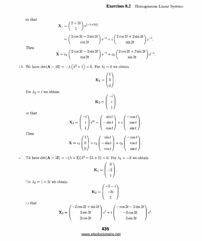
Exercises 8.2 Homogeneous Linear Systems
so that
Xi =2 -I- 2 i 0(-l+2i)t
Then
' 2 cos 2t — 2 sin 2t \ _t
cos 21 \e + l
( 2 cos 2t — 2 sin 21 \ ,X = Ci ) e + c2
V cos 2t J
' 2 cos + 2 sin 2t \
sin 21 J
/ 2 cos 2t + 2 sin 2t \
sin 2t I ("
3 3. Wc have det(A — AI) = —A (A2 + l) =0. For Ai = 0 we obtain
/1\
K i =
For A2 = i we obtain
K 2 =
0
Vo/
f-i\
i
l )
<o that
X 2 =
Then
X = Ci
f-i\
i
1/
/1\
0
Vo/
sin t\
+ i— sin t
V cost J
sin t\ — cos t \
— cos t
cos t
sin t /
+ C2 — sint
cos t J
+ C3 cost
V sin t J
-=-!. We have det(A — AI) = — (A + 3) (A2 — 2A + -5) = 0. For Ai = —3 we obtain
( 0\
Ki =
ror X2 = 1 + 2i we obtain
i-j that
X 2 =
K 2 =
/ — 2 cos 2t + sin2i\
3 sin 21
v 2 cos 21 )
- 2V 1/
(~2-i\
-3*
2 /
e + i
( — cos 2t — 2 sin 2f X
—3 cos 2t
2 sin 2t )
e*.
435www.elsolucionario.net

Exercises 8.2 Homogeneous Linear Systems
Then0\
- 2 1 /
—2 cos 21 + sin2i \
e _3 t + c2 3 sin 21
2 cos 21
— cos 2t — 2 sin 2i \
e + C3
/
—3 cos 2t
2 sin 2t
41. We have det(A - AI) = (1 - A) (A2 - 2A -f- 2) = 0. For Ai = 1 we obtain
/0\
K i =
For A2 = 1 + i we obtain
K 2 =
2
V I/
m
%
w
so that
X 2 =
/1\
i
\i /
Then
X = ci
/0\
2
V1/
e + C2
/ cos t \
— sin t
\ — sin t j
cos t \
— sin t
— sin t /
e + i
el + C3
sin t \
cos t
cos t )
sin t \
cos t
cos t )
42. We have det(A - AI) = -(A - 6)(A2 — 8A + 20) = 0. For Ai = 6 we obtain
/0\
K i =
For A2 = 4 + 2i we obtain
K 2 =
1
Vo j
0
2/
so that
X 2 =
(~i\
0
2 J
,(4+2i)t
Then
X = ci
(0\
1
U /
/ sin 21 y
0
2 cos 21)
sin 2t \
eu + i
ea + c2 0
2 cos 2t J
e4t + c3
— cos 2t N
0
2 sin 21 j
f — cos 21 \
0
2 sin 2t )
At
At
e*.
436www.elsolucionario.net

Exercises 8.2 Homogeneous Linear Syste
Wo have det(A — AI) = (2 — A) (A2 -h 4A -f-13) = 0. For X\ = 2 we obtain
/ 28
K i =
For A2 = —2 -f- 3i wo obtain
-5 I .
\ 25
( 4 -j- 3i
-5
0
so that
X 2 =
Then
/4 + 3A
-5
0 J
( 28 \
4 cos 3t — 3 sin 31 \a(-2+3i)t = -5 cos 31
0
e~2i + i
4 sin 3t + 3 cos 31'
—5 sin3i
0
,-2t
X = ci -5
V 25 /
e2t 4- c2
4 cos 3t — 3 sin 31 \
—5 cos 31
0
e 21 + ca
4 sin 3i + 3 cos 31 \
—5 sin 3t
0
.-21
We have det(A — AI) = — (A + 2) (A2 + 4) = 0. For Ai = —2 wc obtain
( o\
K i = -1
For A2 = 2i we obtain
Ko =
/ —2 —2i\
1 7
so that
X 2 =
Then
/ —2 — 2A
1
1 /
( 0
—2 cos 2i + 2 sin 21 \e2U = cos 21,
cos 2£
—2 cos 2t — 2 sin 2t \
/
sin 21
sin 2t /
X = c-
/ —2 cos 2t + 2 sin 2t \
'1 I 6 4" c2
1
cos 2t
cos 2 /,
+ c3
—2 cos 2t — 2 sin 2t \
sin
sin 2i /
We have det(A — AI) = (1 — A) (A2 + 25) = 0. For Ai = 1 we obtain
/ 25 \
K , = -7
6 /
437
www.elsolucionario.net
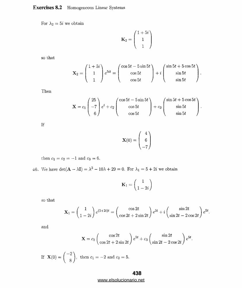
Exercises 8.2 Homogeneous Linear Systems
For A2 - 5i we obtain
so that
Then
If
K 2 =
V 1 )
1 + oi \
1
x, =1 + 5?' \ cos 5i — 5 sin 51 \
cos 51
cos bt J
+ i
25 \
-7
6 /
er + 0 2
cos 5t — 5 sin bt \
cos 51
cos 51 J
- f c3
sin 5t. + 5 cos 51, \
sin 51
sin 51 /
sin ot + 5 cos 51 \
sin 51
sin 51 J
X(0) =
4 \
6
\ -v
then ci = C‘2 = — 1 and C3 = 6.
c6. We have det(A - AI) = A2 - 10A + 29 = 0. For Ai = 5 + 2% we obtain
K i =1 - 2 i
so that
X ! = (54 2-i)* _
1-2*
cos 21
cos 2t + 2 sin 21+ i
sin 21
sin 2t — 2 cos 2t
and
( cos 21 \ ( sin 21X = ci eJ* + c-3 I e
\ cos 2t + 2 sin 21J \ sin 2t — 2 cos 21
51
If X(0) = f j . then ci = —2 and (>2 = 5.
438www.elsolucionario.net
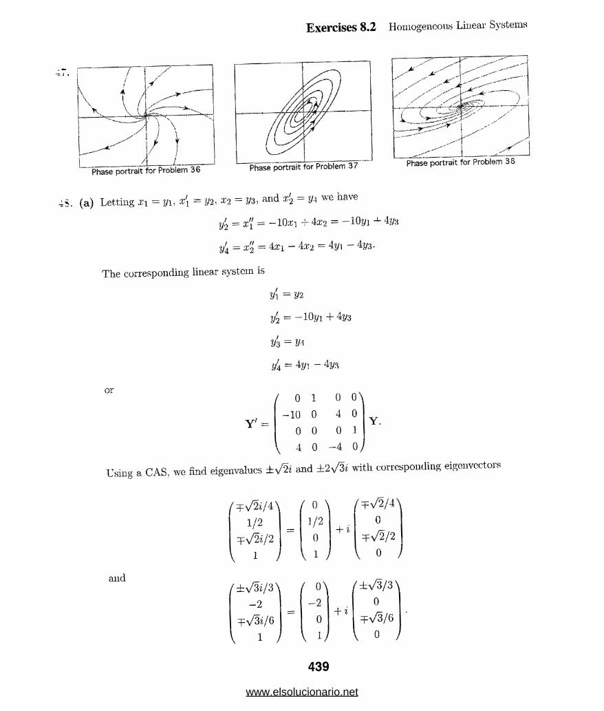
Exercises 8.2 Homogeneous Linear Systems
— f .—
> -
......
......
......
.....
/
x
/
-----------------
y
Np
k._
____
_'1
1 —
j
’...
......
......
.—
) )
A
! ( $
%V
y y , y
s y
- jk'-'""'___-0% SvL__ +— ••
^ SPhase portrait for Problem 38
tS. (a) Letting xi = y\. x[ = 1/2 -, X'l = V z and = va we have
y<2 = x'[ = —lOaSl -r iX‘2 = — lO'jt/i
'</4 = -4 = 4-ci - 4*2 = Ay] _ 4y3‘The corresponding linear system is
2/1 = Vi
y'2 — -10yi + 4 3
?/3 = ?/t
t/4 = 4yi -
or
Y ' =
/ 0 1 0 0\
-10 0 4 0
0 0 0 1
V 4 0 - 4 0 /
Using a CAS. we find eigenvalues ±y/2i and ±2y/2i with corresponding eigenvectors
and
+\f2i(4\ ( 0 ^ /=fV2/4 \
1/2 1/2 0
q=\/2i/2 0+
=fV2/2
1 ) \ 1 > 0 /
f ±\/3i/3 ( °\
( ±\/3/3\
—2 -2 0
+V3i/6 0+ i
+V3/6
1 > J 0 ;
439
www.elsolucionario.net
Exercises 8.2 Homogeneous Linear Systems
Thus
YCO = Cl
■ 0 \ f- V 2/4 \
1/2
0cos y/21 —
0
-V2/2sin V21
I 1 J \ 0 J
+ C2
(~y/2/A\
0
-\/2/2
0 /
cos \/2t +
0 \
1/2
0sin V21
1 )
0\ V3/3\
+ C3-2
0COS 2V 31 —
0
—a/3/6sin 2\/3i
1 I 0
V5/3N( ° )
+ c40
-V3/6cos 2V3£ +
-2
0sin2\/3i
1 0 J l j
The initial conditions yi(0) ■ 0, ^(O) = 1, 2/3(0) = 0, and 2/4(0) = —1 imply c\ = —
C3 = — | . and C4 = 0. Thus,
F> \P\rci(i) = yi(t) = —^ sin \pl1 + -y- sin2\/31
/2 a/3•^2(0 = 3/3 (£) = — — sin \/2t — — sin2\/3t.
O 1U
(b) The second-order system is
or
x'{ = -lOx] + 4. 2
x'2 = 4x\ — Ax?
J ) *Wc assume solutions of the form X = V coscot and X = Vsincji. Since the eigenvalues t:
and —12, = ^j—(—2) = \/2 and cjo = ^ —(—12) = 2\/3. The corresponding eigenv-
www.elsolucionario.net

Exercises 8,2 Homogeneous Linear System
Then, the general solution of the system is
X = ci ( j cos \f2t + C2 j sin \pit + C3 ( ' J cos 2y/3t + 0 4 ( ^ J sin 2\/31.
The initial conditions
X ( 0 ) = Q and X'(0) = ( _ 1)
imply ci = 0, C2 = —y/2/10, C3 = 0. and C4 = -\/3/10. Thus
/2 /3a?i(t) = —— sin \f2t + sin2\/31
10 5
£2(0 = - r- sin V21 - ~ sin 2\/31.5 10
(a) From det(A — AI) = A(A — 2) = 0 we get Ai = 0 and A2 = 2. For Ai = 0 we obtain
P 1 °)VI 1 0 ;
For A2 = 2 we obtain
/ - I 1 | O'
V i -1 | 0,
Then
' I 1
,0 0so that K i =
-1'
-1 1 O'
0 0so that K 2 =
X = C]-1'
1 , e21
The line y = —x is not a trajectory of the system.
Trajectories are x = —c\ + C2 e2t. y = C\ — c^e1 1 or
y = x + 2ci. This is a family of lines perpendicular
to the line y — —x. All of the constant solutions
of the system do, however, lie 011 the line y = —x.
(b) From dot (A — AI) = A2 = 0 we get Ai = 0 and
::)■A solution of (A — AiI)P = K is
P =
K =
"0
so that
X = ci-1
- 02-1’
t +
/ X /■■ . \ // X/
/ / V
i• y
//
/ /*•
/■
/ //
A. / ”
\ /X/
./ \/ \
-1
441www.elsolucionario.net

Exercises 8.2 Homogeneous Linear Systems
All trajectories are parallel to y = —x, but
y = —x is not a trajectory. There are constant
solutions of the system, however, that do lie
on the line y = —x.
50. The system of differential equations is
X \ WX; \ W \ \ x-\ \ xx x _ \ w \ Jhw , \ \ \ x v ,x\ > V \
X X\ \ V1 "' \X \\ \ W \X X X
x 'i = 2X \ + .X‘2
4 = 2x2
£3 = 2.T3
£4 = 2a:4 + 35
4 = 2x5.
We see immediately that X2 — C2 e2f\ X3 = cse2t, and X5 = c$e2t. Then
x ' l = 2 x i + C2&,21
and
so X \ = C2te2t + c i e 21
X4 = 2x4 + c e21
The general solution of the system is
so
C2^e2^ + c\e2t \ 2t
X =
C2.er
c$e2t
c te'2t + c.±e2t
c e2t
X 4 = c $ te 2t + c ^ e 21.
442www.elsolucionario.net

Exercises 8.2 Homogeneous Linear System:
= ci
/1\ (1 ) m
0 0 i
0 _L_e + (‘2 0 te2t + 0 e2f
0 0 0
UJ UJ UJ
+ t'3
( 0\ /0\ m fo\
0 0 0 0
1 v 2t _L_e + c,\ 0 e2* + C5 0 tt* + 0 e2t
0 1 1 0
UJ UJ UJ UJ
= C]Kie.24 C2 K i te2t +
/0\
1
0 e2*
0
UJ
+ CsK-2e2t + C4K^ezt + eg•2t
There arc three solutions of the form X = Ke21. where K is an eigenvector, and two solutions o:
the form X = K te2t + Pe2t. See (12) in the text. From (13) and (14) in the text
/0\
0
K 3ic;2t + 0 e2t
0
UJ
and
This implies
(A - 2I)Ki = 0
(A - 2 I )K 2 = Ki.
o o o f Pl\ / i \
0 0 0 0 0 P2 0
0 0 0 0 0 PS = 0
0 0 0 0 1 Pa 0
ooooo
U s / UJso p2 - 1 and = 0. while p\. p%, and are arbitrary. Choosing p\ = p$ — p4 = 0 we have
443www.elsolucionario.net
o<
Exercises 8.2 Homogeneous Linear Systems
Therefore a solution is
Repeating for K 3 wc find
so another solution is
X =
X =
m
0
p - 0
0
U ;
(l\ / 1 \
0 0
0 «e2,+ 0
0 0
\0/ w
/°\
0
p — 0
0
w
/0\ /°\
0 0
0 te2t + 0
1 0
w v v
..21
,,2i
1. From x = 2 cos 2t — 2 sin 2t, y = — cos 21 wc find x + 2y = —2 sin 21. Then
(x + 2y f = 4 sin2 21 = 4(1 - cos2 21) = 4 - 4 cos2 2t = 4 - Ay2
and
x2 -f 4,ry + Ay1 = A — Ay2 or x2 + Axy + 8y2 = A.
This is a rotated conic section and. from the discriminant b2 — 4ac = 16 — 32 < 0; we see th*'.:
curve is an ellipse.
>2. Suppose the eigenvalues are a ± i@, ,8 > 0. In Problem 36 the eigenvalues are 5 ± 3i, in
Problem 37 they are ±3i, and in Problem 38 they are — 1 ± 2%. From Problem 47 we deduc
the phase portrait will consist of a family of closed curvcs when a = 0 and spirals when a ^
origin will be a repcllor when a > 0, and an attractor when a < 0.
444www.elsolucionario.net
Exercises 8.3 Nonhomogeneous Linear Svste:
N Ohhombgeneoug |4oe& Systems
Solving
dot (A - AI) =2 - A 3
-1 - 2 -AA2 - 1 = (A - 1)(A + 1) = 0
we obtain eigenvalues Ai = — I and A2 = 1. Corresponding eigenvectors are
K , = ( ~ i ) K 2= ( “ lJ ) '
Thus
X c = ci—3'
Substituting
into the system yields
X„ =ai
A
2ai + 3fri = 7
—o,\ — 2bi — —5,
from which we obtain a\ = — 1 and 61 — 3. Then
Solving
det(A - AI) =5 - A 9
-1 11-A= A2 - 16A -r 64 = (A - 8)2 = 0
~.'e obtain the eigenvalue A = 8. A corresponding eigenvector is
3\
Solving (A — 81)P = K we obtain
K =
P =
,1
'2 s
. hus
Xc = Cl ( l ) e8t + C2
'3'leu + r 1 eat
445www.elsolucionario.net
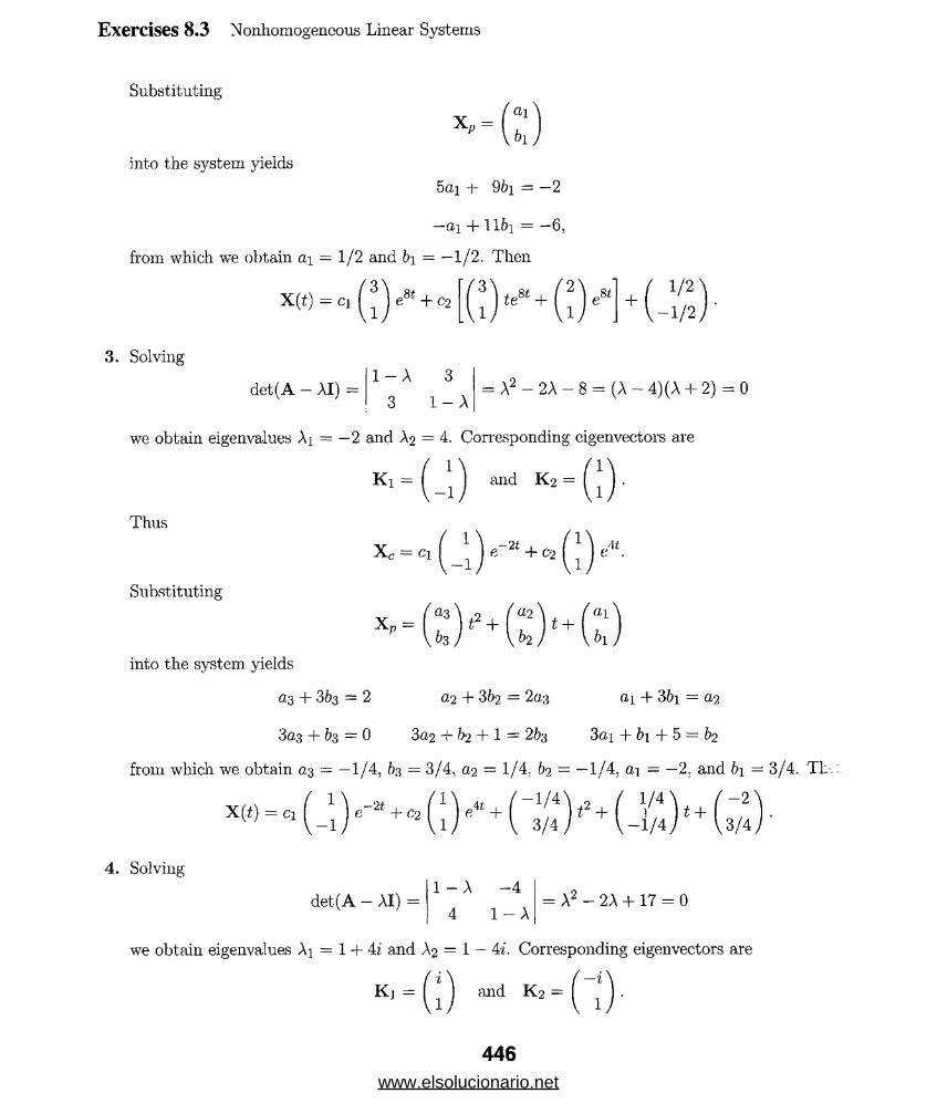
Exercises 8.3 Nonhomogeneous Linear Systems
Substituting
into the system yields
Xp =ai
M
5oi + 9&i = -2
—d\ 4“ 1 lfo = —6,
from which we obtain ai = 1/2 and bi = —1/2. Then
X(t) = c1 l \ e Bt + c2„8iS +
1/ 2 '-1/2,
3. Solving
det(A - AI) =1 - A 3
3 1 - A= A2 - 2A - 8 = (A - 4) (A + 2) = 0
we obtain eigenvalues Ai == —2 and A2 = 4. Corresponding eigenvectors are
* = ( _ ; ) and K , - ( ; ) .
Thus
Substituting
x c = o I ( _ ii ) e- +C2( ; ) e«
:: m z - :into the system yields
a3 4- 363 = 2 a2 4- 362 = 2ag ai 4- 3&i = a2
3a3 + 63 = 0 3(12 4- fa + 1 = 263 3ai 4- &i 4- 5 = &2
from which we obtain G3 = —1/4, = 3/4, a2 = 1/4, 62 = —1/4, fl| — —2. and 61 = 3/4. Tl:
X » = * ( ( 1 ) + ( 3/4 ) *2 + ( —1/4 ) ‘ ■+ ( 3/4 ) '
4. Solving
det(A - AI) =1 - A -4
4 1 - A= A2 - 2A + 17 = 0
we obtain eigenvalues Ai = 1 4- 4£ and A2 = 1 — 4i. Corresponding eigenvectors are
446www.elsolucionario.net
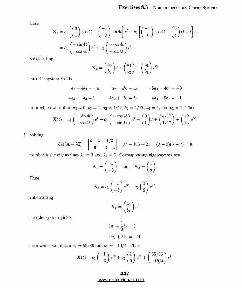
Exercises 8.3 Nonhomogeneous Linear Systems
Thus
Xc = cj ^ I cos At + ( ) sin At 1 \ 0
(‘} + C2
( — sin4t\ , / — cos 4A , = ci 1 e + C2 , e-
V cos At I V — sm At J
Substituting
ki b2 h
into the system yields
a,3 — 463 = —A (22 — 4&2 = —5ai — 46i = —9
4a3 + 63 = 1 4a2 + £>2 — &3 4a 1 — bb\ = — 1
from which we obtain a% = 0, 63 = 1, a-2 = 4/17, 62 = 1/17, a\ — 1, and 61 = 1. Then
X(i) = ci- sin At
cos Atez + o>
Solving
det(A — AI)4 A 1/3
9 6 - A= A2 - 10A + 21 = (A - 3)(A - 7) = 0
we obtain the eigenvalues Ai = 3 and A2 = 7. Corresponding eigenvectors are
» , . ( • ) - k , = ( M .
Thus
substituting
* = u rinto the system yields
3ai + -61 — 3
9 -I- 56i —10
:rom which we obtain a\ = 55/36 and b\ = —19/4. Then
e .
447www.elsolucionario.net
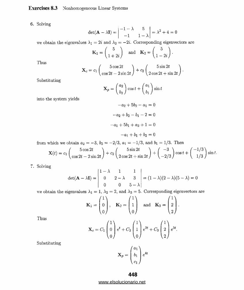
Exercises 8.3 Nonhomogeneous Linear Systems
6. Solving
det(A — AI) =-1 - A 5
= A2 + 4 = 0-1 1 - A
we obtain the eigenvalues Ai = 2i and A2 = —2i. Corresponding eigenvectors tire
' 5 \ . { 5 '
Thus
Substituting
K i = I I and K 2 = ,VI+ 2*7 V 1 — 2*/ 5 cos 21 \ / 5 sin 21
c Cl I cos 2t — 2 sin 2t J 2 I 2 cos 21 + sin 21
X , - ( £ ) « . * + r M - n t
into the system yields
—a2 + 5bo — 0,1 = 0
—02 + h - h - 2 = 0
—<zi + 5bi (12 1 = 0
-at + b\ + 62 = 0
from which we obtain a,2 = —3, 62 = —2/3, a\ = —1/3, and b\ = 1/3. Then
/ 5 cos 21 \ / -5 sin 2t
Cl I cos 2t — 2 sin 2t ) °2 \ 2 cos 2t + sin 2t
-3 \ / —1/3'cos t + I ,
-2/3J \ 1/3,
Solving
det(A - AI) = = (1 - A)(2 - A)(5 - A) = 0
1 - A 1 1
0 2 - A 3
0 0 5 - A
we obtain the eigenvalues Ai — 1, A-2 = 2, and A3 = 5. Corresponding eigenvectors are
/ 1\ /1\ /1\
K i = 0
V O Jk 2 =
Thus
X c = Ci
/1 \
0
W
e' + C*
Substituting
(a\\
bi
Vci /
At
sin t.
448www.elsolucionario.net

Exercises 8.3 Nonhomogeneous Linear
—3&i + bi + C\ = —1
—2b\ 3 C\ = 1
d = -2
from which we obtain ci = —2. b\ = —7/2, and ai = —3/2. Then
into the system yields
X(i) = Ci
/1\
0
/1 \
+ C*2
/ 1\
e2t + C3 e5t +
( —3/2\
-7/2 At,
S. Solving
Vo/ W W -2 /
-A 0 5
det(A - AI) = 0 5 - A 0 = —(A — 5)2(A + 5) = 0
5 0 -A
wc obtain the eigenvalues Ai = 5, A2 = 5, and A3 = —5. Corresponding eigenvectors are
/1\ / 1\ / 1\
Ki - 0
VO/, K 2 = 1
V i/
and K :} = 0
V —1 /
Thus
X c = Ci
/1\
0
V I/
e5t + C2
/1 \
1
V i/
e5* + Qi
1 \
0
V - i /
—5t
Substituting
X p =
f a A
h
V-i)
into the system yields
5ci = -5
5 h = 10
5ai = -40
: jm which we obtain c\ — —1. b\ = 2, and a\ — —8. Then
/1 \ /1\ ( 1\
X(t) = Cx 0
V I /
e5t + C2 1
VI/
+ Ca 0
V - i /
e-5i +
/ - 8\
21-1/
449www.elsolucionario.net
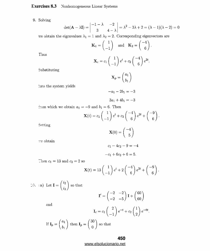
Exercises 8.3 Nonhomogeneous Linear Systems
9. Solving
det(A - AI) =-1 - A -2
3 4 - A= A2 - 3A + 2 = (A - 1 )(A - 2) = 0
we obtain the eigenvalues Ai = 1 and A2 = 2. Corresponding eigenvectors are
- k , = ( - * ) .
Thus
Substituting
X p =a 1
61.
into the system yields
—ai — 2b\ = —3
3ai + 4&i = —3
from which wc obtain a y = —9 and i>i = 6. Then
X(t) = ci-1
jetting
'■.'e obtain
x«» = ( 5jci — 4c2 — 9 = —4
—ci + 6C2 + 6 = 5.
"hen ci — 13 and Co — 2 s o
e2* +-9'
10. ;a) Let I =
and
*2
M .so that
X :Ie = c1 ( _ 2i )e - ‘ + c J 12 \e-6t
If Ipai
6 1 .then Ip =
'30'so that
450www.elsolucionario.net

Exercises 8.3 Nonhomogeneous Linear SysU:::>
i = C lf _ 2i ) „ - , + O2( ^ c-<«+ V 0
'O'For 1(0) = ( j we find c\ = —12 and c-2 — -
(b) «i(t) = i2(t) + k(t) = - U e ^ - lSe~GL + 30.
.1. From
- 6.
we obtain
Then
so that
and
x ' = ( 3 3 ) x+.2 -2 / V-l
$1 3e
, 1 2e* ,
u = / * - * * =
and $ 1 =e f — e~
-11
5e“*dt =
- l i t '
—Qe~f'
x P = * u = ( : ; ; ) t + ( : ; ^
12. From
we obtain
Then
so that
and
From
Xc = c;iGy + c2G)e-‘.$ =
“ d * _ i = ( " 5 * .
■2te~t \ _ (Zte-' + frr*'
2te} J Ct ~ [ 2tel - 2ef
, - . . 0X- = $ U = )t +
p [ 8 V-4
* - ( i : > ( >451
www.elsolucionario.net
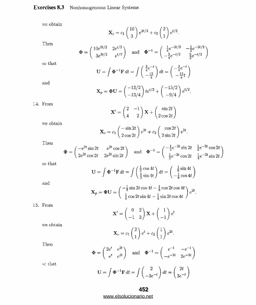
Exercises 8.3 Nonhomogeneous Linear Systems
wc obtain
Then
so that
10\ „/o ( 2'>.c = ci I . „
1 3 / VIX c = ci [ 7 )e3</2 + c2 ' e*/2.
/ 10e3t/2 2e^\ , ( \ e ^ 2 - h ^ 2'
* - [ 3 ^ /2 eif t ) “ d * " “ (- §«- /» ,
U = / * - 1P * = / ( _ J u
3„—i \
t
and
14. From
x ;
we obtain/ — sin 2£ \ 0+ / cos 2t \ 0,
X c = ci ( e^ + ca I e .V 2 cos 2*7 \ 2 sin 2t )
Then
so that
and
15. From
we obtain
Then
sc that
/ —e2tsin2t e2*cos21\ , f ~ke 2tsm21 \e 2
U e 2‘ cos2« 2e2‘ Sin 2 ( j “ (, I c-2*cos2t \e~2
U = / * - > F * = / ( * “ * ) , * _ ( f Sin4tN)./ J \ sin it J \ — | cos 4f /2 1
/ — A sin 2t cos i t — | cos 2t cos At \X„ = * U = 8 8 )e* .
\ | cos 21 sin 4i — | sin 2£ cos /
t
e */ 2e « \ _1 / e& — * O-f an(i # = I O, r>j
\ e* e2t I \ —e u 2e 21
1 cos 2t
1 sin 2i
452www.elsolucionario.net

Exercises 8.3 Nonhomogeneous Linear Syst
and
16. From
we obtain
Then
so that
and
I". From
we obtain
Then
so that
and
H'om
~e obtain
X p = $ U = [ _ ] tef +'3'
2 V 3et.
X ' = ( -1 3) X + ( e -
f 2ef e2t\ , ( e t -e
* - e< «“ J ^ = -e-2‘ 2.-*
f . t ( 2e~t -e-‘u \ ( - 2e-t + \e-4t'
/ 3t - 3
* - ( !
Xc = Cl ( i ) e3t + C2 ( l ) e 3‘-
_ 2e-3n , lc-3« J e -
I «* e-3‘ \ - le * !« » .
/■ , /■ / 6£e 3£ \ / —2te 'il — 4e
= ete* ) * - ( 2 ^ - P .
Xp = * U = ( “ 12W ^ _4/3Ni0 J V—4/3,
x ...,453
www.elsolucionario.net

Exercises 8.3 Nonhomogeneons Linear Systems
Then
so that
and
$ = ' 4e;tt -2 e3* and $ 1 =
U = / 3>_1F dt —
1 r-Zl I e>-'it -6 3
_Lo3t 2 3*6 3
Je”4f + 3fe"2*'- 5 * “ +
eft ~- . ± e-i t - U e- * - 1 p -2*
24 6 12*'_ i p2t , 1^4* _ _Lp4t
12 + <rf' 24e'
Xp = $ u = —ie* — W- I . - - V
19. From
wc obtain
Then
so that
and
X' =-2 - l ) X + ( l ) e' '
X c — ci- 1
et
ei — c2
er te —e} be* — tef and $ 1 =
e_t - 2te“* -2te, - t ■
2e 2e~t
U Fdt = ' 2e'2t - 6te-2f \ ^ ^ e"2* + 3te~2t—'21
XP = « U =
20. From
we obtain
Then
so that
and
* - ( - 2 _ 2Xi \ * / o
te +X c = c-i | | e1, + C2- 1
$ =
U
e te}—e} ~ ,
= J ®~1F d t = I
and $ 1 -
1/2/
e~f - 2ie“* -2te~*'
2e“* 2c-f .
3e_i + 4£e-t \2e-i dt =
-2e-
X„ = $ U = - 5
454www.elsolucionario.net
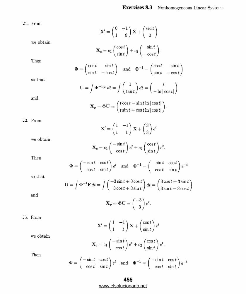
Exercises 8.3 Nonhomogeneous Linear System-
21. From
we obtain
Then
so that
and
22 . From
we obtain
Then
so that
and
-i. From
we obtain
Then
/ cos t\ ( sin t ' X c = Ci + C‘2 IV sm t I \ — cos t
/cos t s in £ \ f cost sint= I and $ — IV sin t — cos t j V sin t — cos t
U = f $ - 1F d t = [ ( 1 fJ J \tan t) \ — In | cos t|
/ tcost — sintIn | cosi| \— i U —— I 1\ t sin t + cos t In | cos t \ J
/ — sin A t ( cos A t X c = ci e + c 2 e .V cos t ) V sm t }/ - s i n t cos A , , , / - s i n t. cos A <& — j e and <& 1 = I eV cost sint J \ cost sint )
f i / 7 —3 sin i- i-3 cos AU = / $ ~ 1F d t = i =J J \ 3 cos t + 3 sin t J
3 cos t + 3 sin t ' 3 sin t — 3 cos t
i w s y/ — sin A t / cost \ t Xc = Ci I + K + c2 . e*. \ cos t j \ sm t j
/ - s i n t cost \ , , , / - s i n t cosA t <p = e and 3> = eV cos t sin t j \ cos t sin t
455www.elsolucionario.net
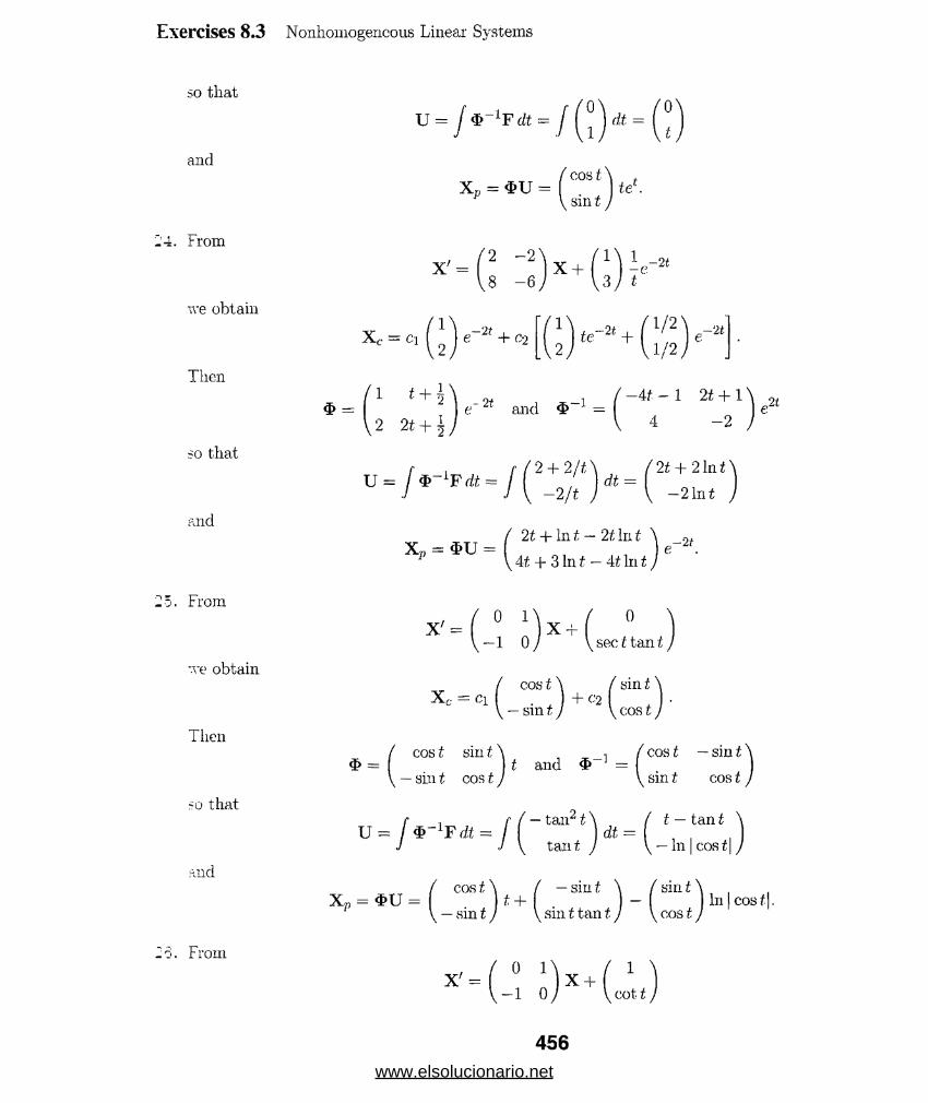
Exercises 8.3 Nonhomogeneous Linear Systems
so that
and
24. From
w e obtain
Then
so that
and
25. From
A_e obtain
Then
so that
and
26. From
x ' - f i : « ) x + G ) r “
Xc = Cl ( 2 } e~2t + c-2 t e ~^ + 1 ) e_ 2) V1/ 2 /-21 21
$ = ■ 2t and $ 1 = -it - 1 2t + 1 '
/ 2t + In t — 21 In t \ 9#. X p = $ U = I e .1 \ At + 3 In f — 4t In t )
X f = ( 0 M x + f 0 'V —1 0 / \ sect tan i
'21
2t + 21n A—21n£ J
X c = C! COS t \— sin 11 + 02
sin Acos t ■
( cos t sin t \ _i3> = ) t and\ — sin t cos t J
U = / * _1F dt = / lefttan tcos t \ f — sin t
\ sin t tan t
' cos t — sin t \ (sin t cos t J/ t — tan t \\ — In | cost| /
7 ) t +sm t )sin t \ cost / In | cost|.
x ' = ( - ° i l ) x + L u
456www.elsolucionario.net

Exercises 8.3 Nonhomogeneous Linear Syst
we obtain
Then
so that
and
From
we obtain
Then
so that
.■ind
( cos t \ /sin t' X c = c\ I . , + c2 (V — sm t J \ cos t.i cos t «in t \ i / cos t — sin t$ = and =V — sin t cos t V sin t cos t
U = / = [ ( ° \ d t = ( °J J \ csc t J \ In | csc t — cot 11
/ sin t In | csc t — cot t\ \X p = $ U = ( .V cos 1111 | CSC t — cot 11 J
X ' = ( 1 2 W\ —1/2 1 / \sec t J( 2 sin t \ i ( 2 cos t \ ,X , = c , ( e‘ + c2 e*.\ cos t ) \ — sm t )
( 2 sint 2 cost \ t , /^ s in t c o s i\$ = ) e* and = ( ' e_tV cosi - s i n t ) V^cosi - s i n t j
U = f ^ - 1F d t = f ( 2 2<J \ i cot i — tan i / j In | sin £ j + In | cos £| /, 3 sin t \ . ( cos t \ t , / 2 cos t \ f , , .
X" = * U = l l c 0si j te + ( - l - t j e la |sin(| + \ - sin t J C ln|C0S(|':rom . / I —2 \ /tan A
* “ ( i - J x + ( i )_'e obtain / cos t — sin t \ ( cos t + sin t '
www.elsolucionario.net
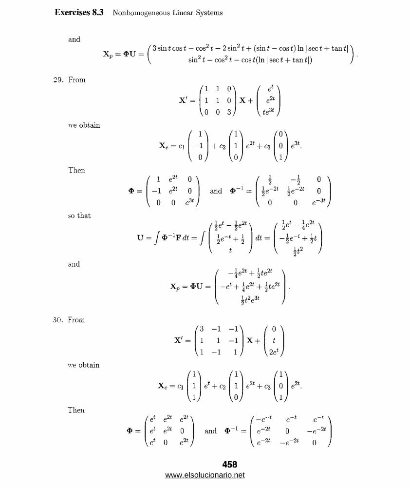
Exercises 8.3 Nonhomogeneous Linear Systems
and/ 3 sin t cos t — cos21 — 2 sin21 + (sin t — cos t ) In | sec t + tan 11 \ sin21 — cos21 — cos i(ln | sect + tant\)
29. From
we obtain
Then
so that
and
X' =1 1 o\ 1 1 0
\0 0 3 /
f ef \X + _2t
tes t )
Xc = ci1 \
-1
0 /+ C2
1 \1
Vo /e2t + eg
/ 0 \0
VM
$ =
1
— 1 eV o o
2t
21 0 \ 0
e3*/
U = j $ ~ 1'Fdt = J\
l e - t + 1 2 + 2
i /
„3t
-e 2t |e 2t2 0
dt —
0 \0
-at0 e-'w/
Je* - |e 2t \— 5e_' + 5*
¥ 2 ■
Xp = $ U-J e 2* + ite2t: \
-e* + ±e2i + ±te2f ±t2eM
30. Jrrom
we obtain
Then
X' =3 - 1 - 1 \ 1 1 - 1
U - i i /x +
° \ t
W )
/ 1 \x c — c\
( 1 \e + C2
/ 1 \e2t + c3
„2tV i / V o/ V l/
( e4 e2* e2,: N /-e" * e~f e“* \$ = ft2i
0 and = ( -2t.0 - e ~ 2t
U* o e2t) \ e~2t - e - 2t o y
458www.elsolucionario.net

Exercises 8.3 Nonhomogeneous Linear Syste::.-
so that
andU = j$~lFdt = j - t—2e -te~2i dt = -te~l -
2e\ie
Xp = $ U = / —i / 2 \ - l
\ —1/ 2 /t +
—3/4 \ -1
V -3 /4 y+
/ 2 \ 2
\ o /e* +
we obtainand
X' = ( - l _3)X+(S)e2T
e4t e2/. = J e -
i c “» ie-
X = $ $
'21(0)X(0) + $ J* QFds = & ■te2< + ( X>\ e2t + 2 £e,4t
+ $
.At.
trom~e obtainMid
X 'J1 -Mx+flA' u - i ; y i/* ,
x =
Lot I = so thatI '= -11 3'
3 - 3/100 sin t \ I+( 0 )
1 'Ic — Cl ( g J 6 2t + C2 - 121
e~l + 21\
2 \2 te*.\2/
e_2t + 2t - 1 \ e2* + 2t. — 1 /
459www.elsolucionario.net
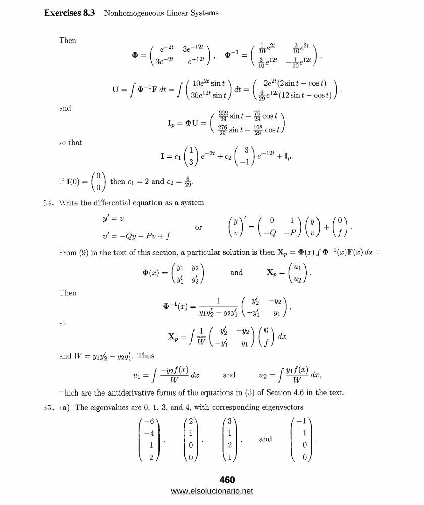
Exercises 8.3 Nonhomogeneous Linear Systems
Then$ -
3e- 21 _ e- 121 = _Lp2l 10 eS_A21 10t
_3_ ‘2f • 10 €
106 ‘
U = / * - * * = / ( 10e2t sint \ / 2e2t(2sint - cost) \ 30e12* sint / * \ Jjg12iC(12siiif - cost) j ’
ind
?o that1
^ sin t — cos t ' — sin t — cos t ,29 29
I = M 3 K * + c2 — 1 e + 1 p .
O'If 1(0) — ( n ) then ci = 2 and e2 =S4. Write the differential equation as a system
y’ = v orv' - -Q y - Pv + f
rrom (9) in the text of this section, a particular solution is then X?, = <1>(.t) / $ _1(a;)F(.x) dx' u i \
0 1 ' - Q - p .
_ hen# ( * ) = r ; *
V 2/1 Vz.
*~\x) =and
yiy2 - V2y[
X p =
y2 -y-2
U2.
X, = [ — ( * J w V-yi
V ~ y \ y\
y2\ / o 'yi y i f . dx
ciid W ~ yit/2 - y2X/i- Thus•ui - I
~V2f(x)w ~~ 2 J wdx and dx,
“iiicli are the antiderivative forms of the equations in (5) of Section 4.6 in the text. 3 5 . i a) The eigenvalues are 0; 1. 3, and 4, with corresponding eigenvectors
/ —6 \ / 2 \ / 3 \ / —1 \- 4 1 1 1, and
1 0 2 0
2 J VV u J 0 /
460www.elsolucionario.net
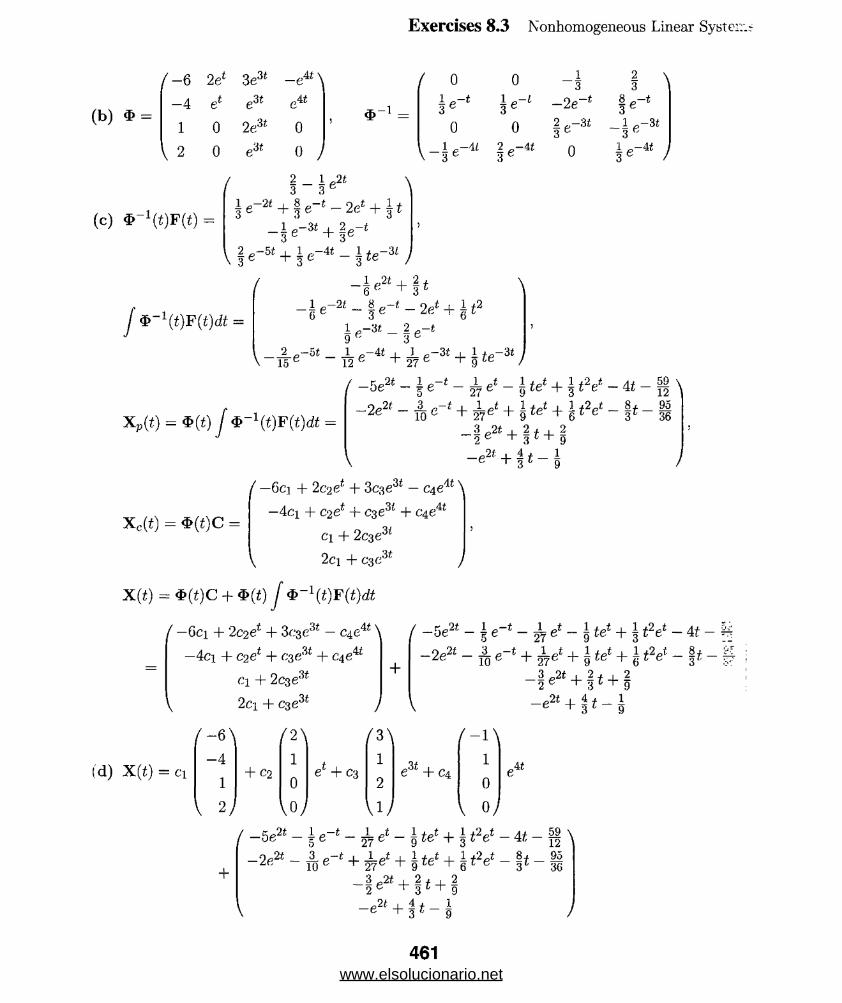
Exercises 8.3 Nonhomogeneous Linear Systcr:'.-
- 6 2e* 3e3* —e4*\ ( 0 0 13
* 'l-4 e* e3* e4* A-1 —i e-t 3 c
l e~L3 - 2e_t 8 ^-*
3 e
1 0 2e3* 0 ; ^ — 0 0 2 —3t3 e
_ I P-3t 3
2 0 e3t o ) \ - - L P-41 3 e' 2 _-4*
3 e 0 | e - 4* /
(c) 4>-‘ («)F(<) =
2 JL3 3 e
| e-2* + | e- * — 2ef’ + j t 3 e : + h~*
V | e 5t + ^ei .-4* _ l te-3i
j $ _ 1(t)F(t)dt_ i Pa , _
6 + 31 p-2 t 6 e | e“* - 2e* ±f26 L
\ _____________________________ L p -
V 15 e 12 e
1 *-3t9 6
-4t
2 e-t 3 e
+ 27 e
X„(*) = *(<) f* -\ t)F (fid l =
/ —6ci + 26*26* + Scjje3* — C4e4t \
—5e2* — | e * - ^ e* - ± te* + ± t2e* — 4t — f | \_ 2e2t - A «-* + JLft + / V _ 8/ _ M
•6e 1 0 ° ^ 27 t 9 te + 6 “ 3 36_ 3 e2* , 2 , , 2 2 c t j i t 9
_ e2t i | + _ 1 e t o o Q
X c(t) = &(t)C = -Aci + c2e* + C3e3i + c eAtci + 2C3C3<2ci + j
X{t) = #(t) C + $(t) j <&_1(t)F(t)dt
id) X(t) = ci
—6ci + 2c2e* + 3c3e3t — c±e4t \ —4ci + c2e* + ese3* -f- C4e4*
ci + 2c3e3*2ci + C3e3t )
/ —6 \ / 2 \1
+
—5e2t — e * — ^ e* — g te* + g t2e* — 4t - - 2e2* - & e“* + ^e* + ± te* + ± f2e* - ft
_ 3 e2 t + 2 < + 2
—e2* + 11 — A
-4
1
2 /
+
+ C20
voye + C3
/ 3 \1
2
v iye3* + C4
/ - 1 \ 1
0
o y
„4t
_ 9 p 2f - i p - ^ x J-p* + I f(!i + I +2 t _ 8 f _ 9 oAt, ^ c T 27l T 9 1/1 T 6 ^4* ■3*
59 \ 12
36- 2 e2i + 2 f + 2 2 e ^ 3 6 ' 9_+ 4 * 1e -f 3 c g
461www.elsolucionario.net
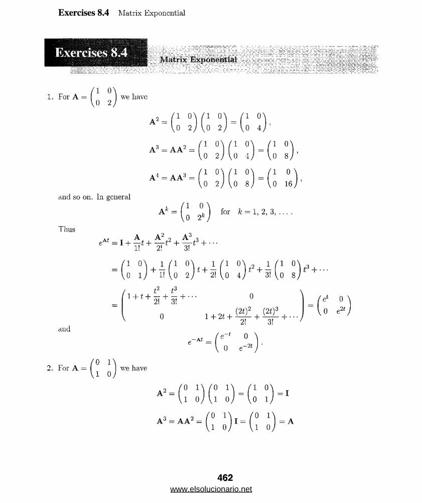
Exercises 8.4 Matrix Exponential
Matrix Exponential
/ I 0 \1 . For A = we naveVO 2
A 2 = 1 0 \ f l 0
,0 2 M o 2
A3 = AA2 =
1 O' 0 4.
1 0 W 1 0
0 2 J I 0 1
A i = AA3 =1 0 \ / I 0
0 2 J lo 8
1 0 \ 0 8 j1 0 ' 0 16
and so on. In generalA* = '1 0
0 2kfor k = 1, 2, 3, . . . .
ThusA+ _ A A2 2 A3 ■, eA i = i + _ t + _ t 2 + _ t3 +
1 O'o i ) + M o 2 ) * + i u I r + ^>u s j *
/ 1
1 + t + 2! + 3! +
and
0
, 0 (2 t f (2 t)3 1 + 2t +
e - Ai =2!
-f 0
\
. . . j
„-21
2. .tor A 0 1 ’1 0
we have
A = 'o in /o in _ / i o'i o J u o J “ v o 1
= i
a 3 = a a 2 = ( ! J ) i = ( i o) = a
462www.elsolucionario.net

Exercises 8.4 Matrix Exponcr.-
A4 = (A2)2 = I A 5 = AA4 = AI = A,
and so on. In general,A K =
Thus
k _ j A, k = 1, 3, 5, . . . I. k = 2, 4 6 ........
and
Af T A A 2 2 A 3 o e*‘ = i + _ t + — ^ + —
= I + A« + i f t 2 + i A r ’ + .- .
= I ( 1 + 5!i2 + i ! i4 + - ) + A (*+ l <3+5if5 +
/ cosli t sinh t \= I cosh t + A sinh t = \ sinh t cosh t J
1. ror
- A t ( C0SM—0 sinh(—t) \ sinh(—t) cosh (—i)
A =1 1 1 \ 1 1 1
V -2 - 2 —2 /
cosh t — sinh t ' — sinh t cosh t
1 I 1 \ / 1 1 i \ / 0 0 ONa 2 = 1 1 1 1 1 i = 0 0 0
-2 - 2 - V V- 2 - 2 - 2 J u 0 0).us, A3 = A4 = A 5 = • • • 0 and
/ I 0 0 \ ( t A t + 1 t t \eAt = I + At = 0 1 0 + t t t = t t + 1
u 0 l j \ - 2 t - 2 1 ~2t { - 2 t - 2 1 -21 -j-1 J
A =/O 0 0 \
3 0 0U 1 o )
463www.elsolucionario.net

Exercises 8.4 Matrix Exponential
.ve have
(0 0 0 ^ (0 0 0 \ (0 0 ONA 2 = 3 0 0 3 0 0 = 0 0 0
u 1 0 ) U 1 o j u 0 0 )(0 0 0 \ (0 0 ON (0 0 ON
A 3 = AA 2 = 3 0 0 0 0 0 = 0 0 0
u 1 o j u 0 o j u 0 0 /Thus, A 4 = A 5 = A 6 = • • • = 0 and
sAt = I + At + - A2f2
1 0 0 \ = 0 1 0
\0 0 1 /5. Using the result of Problem 1,
X =
6 . Using the result of Problem 2 ,
/ 0 0 0 \ 3f 0 0
t 0 /
0 0 ON f 1 0 ON0 0 0 — st 1 0
l 'it2 \ 2 1 0 0 ) \ ' t" + 51 t 1 /
er ( 0 e
cic2
= Cl + C-2
/ cosh t sinh t \ f ci \ ( cosh t \ / sinh t \ \ sinht cosh t J \C2 J \ sinht J \cosh t J
7. Using the result of Problem 3./ t + l t t \ / c A
X = t t -1- 1
- 2t - 2 tt
-2t 1 JC-2
VC3 /= Cl
( t + w t
- 2 1 j+ C-2
t \ t + l - 21 J
+ C3
t \ t
V —21 + 1 /S. Using the result of Problem 4.
1
X = 3f0 0 \ 1 0
' t2 + 5t t IJ
fc,\c2 C3 /
Cl
1
31\%t2 + 5 t /
+ C2
/ 0 \1
\ t /+ c3
/ 0 \0
V i/9. To solve
x ' ^ 1 QN) x +Vo 2 / v - l
464www.elsolucionario.net
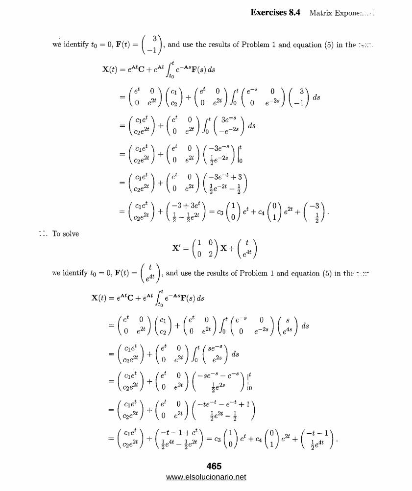
Exercises 8.4 Matrix Expone'
we identify to = 0, F (t) = ( J, and use the results of Problem 1 and equation (5) in the t
X(t) = eAtC + eM f e-AsF(s) dsJtf)
0
~ -2 s- 1
ds
, To solve
C]_eot21coe
C\ec21c-2e
c\eLC2e21
el 0 \ 0 e2t)
0 \0 e2t)—3 -i- 3e*1 _ l p2t2 2 -
m :I p —2s 2
—3e_t + 3'Ip -2*_ 1 2 2 /
c3 | 0 I e +C4
X ' = ( o l ) X +
„2i
we identify to = 0, F(i) = f 4i I. and use the results of Problem 1 and equation (5) in the
X(t) = eAtC + eAt t e_AsF(s) ds•ftn
www.elsolucionario.net

Exercises 8.4 Matrix Exponential
11 . To solve
x ' = ( " i ) x + ( i
we identify to = 0, F(t) = ^ . and use the results of Problem 2 and equation (5) in the tex:
X(t) = eAtC + eAt /* e_AsF(s) ds Jtof cosh t sinh t \ / ci \ / cosh £ sinh t \ rt / cosh s — sinh s \ / 1 \ ^\ sinh t cosh t j \ c-2 ) \ sinh t cosht / -A) \ — sinh s cosh s j \ 1 /
nh t \ rt
3sh t ) Jo
inh t \ / cosh t sinh t \ / sinh s — cosh s Dsh t J \ sinh t cosh t J \ — cosh s + sinh s
' ci cosh t + C2 sinh A / cosh t sinh £ \ rt / cosh s — sinh s \ ci sinh t + C‘2 cosh t J \ sinh t cosh t J Jo \ — sinh s + cosh s )ci cosh t + c-2 sinh £ ci sinh £ + C2 cosh;
/ Ci cosh t + C2 sinli i \ / cosh t sinli t \ / sinh t — cosh t + 1
\ ci sinh t + C2 cosh t J \ sinh t cosh t J \ — cosh £ + sinh H I/ Ci cosht + C2 sinht \ ( sinh21 — cosh2 t + cosht + sinht \\ cj sinh t + c-2 cosh t j \ sinh21 — cosh21 + sinh t + cosh t J
/ cosh t \ / sinh t \ / cosh t \ / sinh t \ / 1 \1 \ sinh t J~*~2 \ cosli t j \ sinh t J \ cosh t,) \1/
/ cosh t \ ( sinh t \ / 1 \= CSV sm h (J+C4 lc o s h ( J ’ l>l j '
1 2 . To solvex '= (° 1N) x + f coshtN)
\1 0 / V srnhi/
we identify to = 0 , F(i) = ( S }, and use the results of Problem 2 and equation (5) inV sinh t JX(f) = eAtC + eA t l ' e~AsF(s) ds
J t.Q
( cosh t sinh t \ f Ci \ ( cosh t sinh t \ rt / cosh s — sinh s \ / cosh\sin ht cosht ) \C2 J \sin ht cosht / Jo \ — sinh,s cosli.s / \ sinli.*
466www.elsolucionario.net
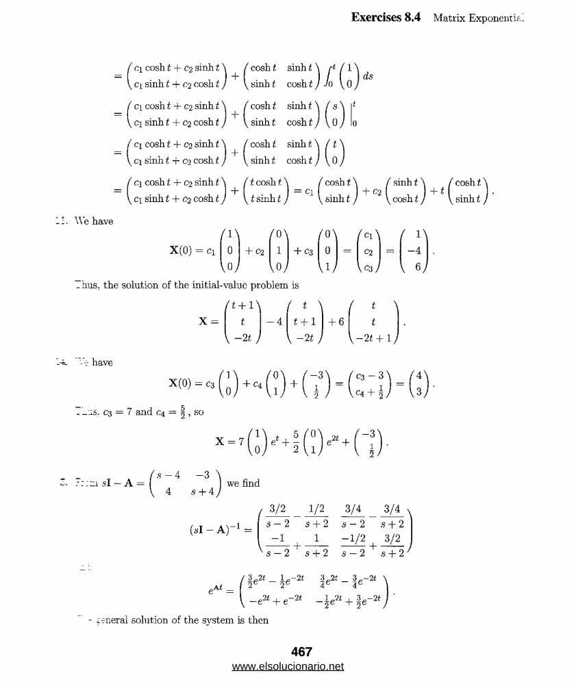
Exercises 8.4 Matrix Exponential
c\ cosh t + c-2 sinh t \ / cosh t sinh t \ /■* / 1 \ Ci sinh t + c.2 cosh t / \ sinh t cosh t ) Jo \ 0 /
/ ci cosht + C2 sinht \ ( cosht sinht \ / s \ *\ ci sinh t + C2 cosh t J \ sinh t cosh t J \ 0/ ci cosh t + C2 sinh t \ / cosh t sinh t \ f t\ ci sinh t, + C2 cosh t J \ sinh I cosh t J \ 0/ ci cosh t \ ci sinh t + C2
+ C2 sinht \ ( t cosht \ ( cosht \ f sinht \ f cc + C2 cosh t ) \ t sinh t J 1 I sinh t j 2 \ cosh t ) I si
cosh t ' sinhf
We have
X(0) = ci
/ 1 \0
Vo/+ C2
/ o \1
V O /
/ 0 \+ C-3 0
V I/_ hus, the solution of the initial-value problem is
f t + l \ ( t \X = t
V - 21 )t + 1
V - 2 t j+ 6
(<*\c2.
\<%)
t
1 \ - 4
6 /
"-4. haveX (0) = c3 f ^ + c 4 f ^ + f
"-US. C3 = 7 and C4 = | , so0
X = 7
1
C3 — 3 , c4 + 5 .
ic: e2t + -3 '• 3 -
"4'
-:: ui 51 — A =' s - 4
s + 4 we find3/2 1/2 3/4 3/4
s — 2 -I- 2 s — 2 s -j- 2
eAt =_ 1 - 2i
2 2
—e2< + e_2t3*2t _ 3,-2* 4e 4
, 3 .-2 i 2 ^ 2
- iriieral solution of the system is then
467www.elsolucionario.net
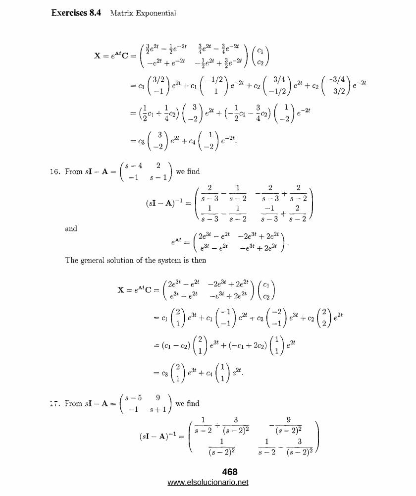
Exercises 8.4 Matrix Exponential
X = eAtC =lp 2 t _ 1 . - 21 3 '2 t _ 3 - 2 1 2 2 4 4
—e2t + e- 2t _ l e2* + 3e-2* / Vc2.
d 1
^ 2 “ ' 4 (= (~ c1 + 7^2 3 ) e21 + ( 1 _ S ) / 1
( s - A 2 \16. From «sl — A = we findV - 1 5 - 1 7
/(si - A )-1 =
andeAt =
s — 3 s — 2 s — 3 s — 21 1 ~ l 2Vs- — 3 s — 2 s — 3 ’ s — 2 y
' 2 e 3/' — e 2* — 2 e 3f + 2 e 2i \
V e3/ - e2* —e3f + 2e2t J The general solution of the system is then
X = eAiC = '2ei t - e ? t - 2e3* + 2e2fe3/ - e2* — e3t + 2e3f , r>*2t c2 .
e2‘
= (Cl - C2) I I e M + ( - C l + 2 c2)~2t
17. From s i — A = s — 5 9 ' - 1 ,s + 1
wc find
/ 3
(.si-A )-1 = s - 2 (s — 2)2
1
V (J--"2?
468
(* - 2)2
1 3
s-2 ~ (8 - 2)2 1
www.elsolucionario.net
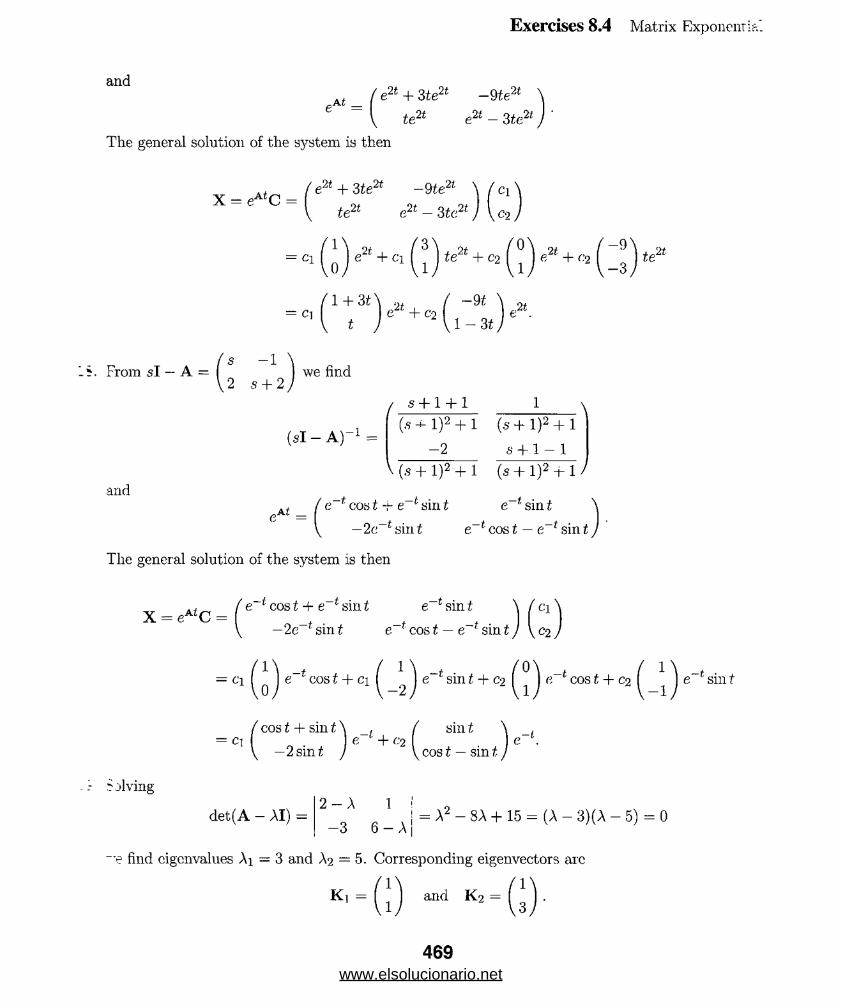
Exercises 8.4 Matrix Exponential
andeA* =
' e2t + 3 te2t - 9 te2t2t e2t - 3te2*te
The general solution of the system is then
X = eAtC = e2t + 3 te21 -9 te2t Clte21 021— 3te2t J I co
ci [ * 1 e2t + ci te2* + c2 f e2t + c2 te'it
( s - 1 \From s i — A = we findV 2 s + 2 /
( s i - A ) -1 =/ s + 1 + 1 1
{s + l )2 + 1 (s + 1)2 + 1- 2 s + 1 - 1
andeA* =
V(s + 1)2 + 1 (s + l )2 + 1 / ' e~f cos t + e~L sin t e~f’ sin t
e t cos t — e r sin tThe general solution of the system is then
X = eA*C = ’ e * cos t + e * sin t e f sint-2e * sin t e * cos t — e * sin t :
= ci e * cos t + c\ e t sin t + co a 1 cos t + c-2 e *sinf
( cos t + sin t \ci sin t -t• I c " + c2 I \e \\ — 2 sint / \co st — sint
det(A — AI) — 2 - A 1
- 3 6 - A = A2 - 8A + 15 = (A - 3)(A - 5) = 0find eigenvalues Ai = 3 and A2 = 5. Corresponding eigenvectors arc
K , = n md K2 = n .
469www.elsolucionario.net
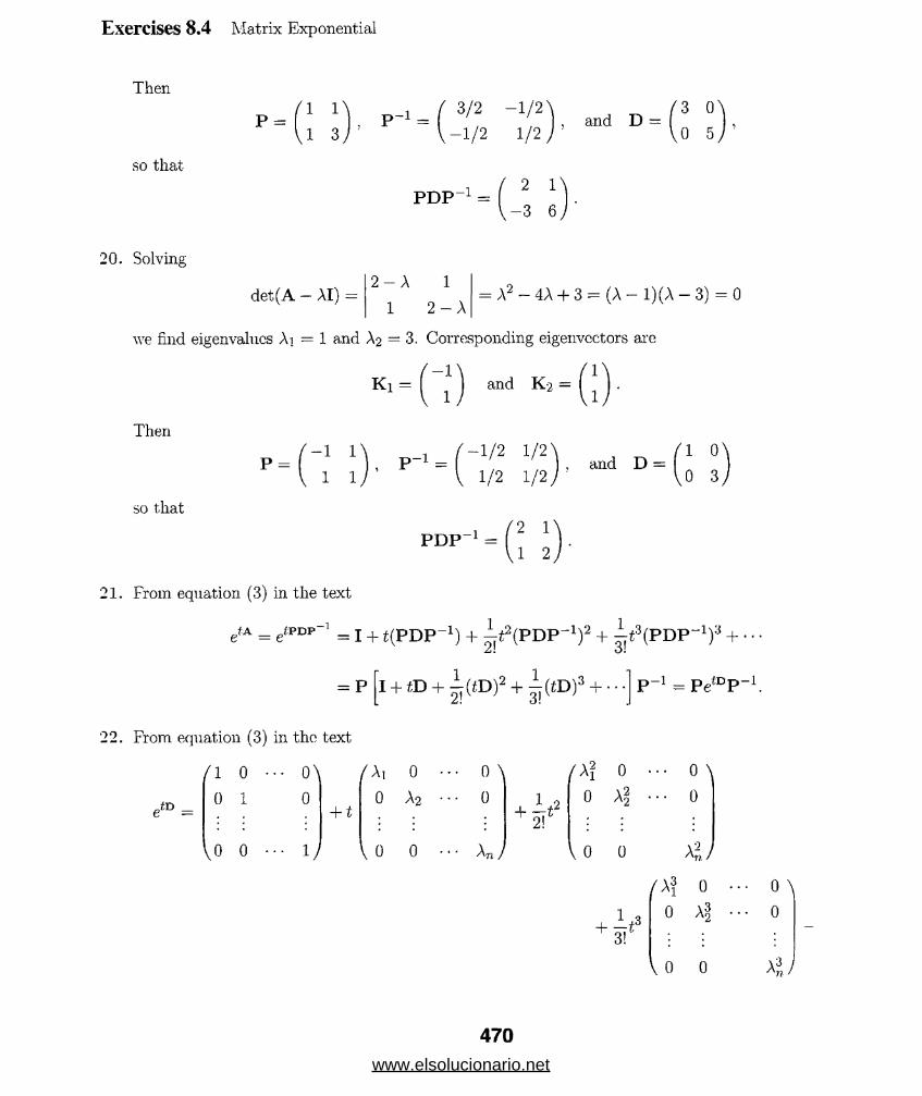
Exercises 8.4 Matrix Exponential
Then
so thatP = 'i r
1 33/2 -1 /2 \ / 3 O'and D ^- 1/2 1/2 0 5
2 1 ' -3 6
2 0 . Solving2 - A 1
1 2 - Awe find eigenvalues Ai = 1 and A2 ‘ 3. Corresponding eigenvectors are
det(A - AI) = = A2 — 4A + 3 = (A - 1)(A — 3) = 0
K i = ( 1 ) and K 2 = ( 1
Then
so that
-1 1
1 1
—1/2 1/ 2 ' . 1/2 1/ 2 ,P = I 1 , P -1 = I ] , and D = 1 O'
0 3
P D P -1 = '2 1 ' 1 2
2 1 . From equation (3) in the texte tA = g fP D P 1 = ! + t ( P D P - i ) + I ^ P D P - 1 ) 2 + ^ ( P D P * * 1) 3 +
Zl o!
= p I + iD + i ( t D )2 + i ( « D )3 +3! p -1 = PetuPiD r»— 1
2 2 . From equation (3) in the text( 1 0
0 1
yo 0
0 \0
1 J+ t
(M 0
0 A2
Vo 0
0 \ 0
An )
/A? 01 0
+ s ‘-
0 • 0 \Af • . . 0
0 A2JA3 0 • • • 0 \
- 13 3!0 A3 . . . 0
1 0 0 A l )
470www.elsolucionario.net
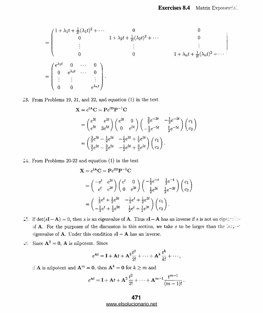
Exercises 8.4 Matrix Exponent:?.!
1 + Ai* + 2t(Ai£)2 + • • • 0
0 1 + A2t + ^(Aat)2 +0
0
( e\ it 0
0 0
0 0 \ 0
gAnt JVo o
23. From Problems 19, 21, and 22, and equation (1) in the textX = etAC = Pe*DP -1C
„te
3 JH 2
3 ~3t
e5> \ .f e3t 0
3eu J I 0 eS:U5 i 1„3t~ 2 ~2e -'iJ>l 1-31~ 2 ~2e -
-4, From Problems 20-22 and equation (1) in the textX = etAC = PefDP _1C
—e t e3/-\ / e*e f c'V \ 0
I et 2 C + 1P912 —
_ 1 J2 + 1 p9t2
IT. If det(sl — A) = 0, then s is an eigenvalue of A. Thus s i — A has an inverse if 5 is not an cige:_
of A. For the purposes of the discussion in this section, we take s to be larger than the Ij eigenvalue of A. Under this condition s i — A has an inverse.Since A3 = 0 , A is nilpotent. Since
eAt = I + A t + A 2l~ H------ j- A k + • • •,2! k\
:f A is nilpotent and A m = 0 , then A k = 0 for k > m andt2= I + At + A2 — + . . . + A'771— 1_f_____
(m - 1)!
471www.elsolucionario.net

Exercises 8.4 Matrix Exponential
In this problem = 0. soof*eAt = I + At + A2 — =
1 0 o\ ( - 1 1 i \ / - I 0 1\0 1 0 + - 1 0 1 £ + 0 0 0
\o 0 i j v - i 1 V l - l 0 1 /(1 — t - t 1/2 t t + t 2/ 2 \
2
- t 1 t - t - t 2/ 2 t 1 + t + t'2/ 2 )
and the solution of X! = AX is
X(t) = eAtC = e- A tf c i \
C*2c i ( l - t - t 2/2) + C2t + Oi(t + t2/2) \
-Cit + C2 + C3\C3 / \ c i ( —£ — £2/ 2) + a t + 3(1 + 1 + tl j 2) /
27. (a) The following commands can be used in Mathematical A = {{4 , 2 },{3 , 3 }} : c = {c l , c2}; m=MatrixExp[A t]; sol=Expand[m.c]Collect [sol, {c l , c2}]//M atrixForm
The output gives
K() = c, ( _ 3 e. + 3e6t) + , 2 ( 3 el + | e6t) .The eigenvalues are 1 and 6 with corresponding eigenvectors
(1) w,d (O'so the solution of the system is
fitor
x(t) = —2b\e} + b‘2eQt
y(t) = 3 i ef + b‘2^yt.If we replace 61 with — ic i + I a and b2 with |c i + Ic2, we obtain the solution found u-x '.) o o o *matrix exponential.
472www.elsolucionario.net

IJ(b) x(t) = c\e~2tcost — (ci + C2)e~2tsint
y(t) = C2e~2t cos t + (2ci + c-2)e~2t sintS. x(t) = ci(3e_2t — 2e- t ) + cs(—Qe~2t + 6e_t)
y(t) = C2(4e-2f — 3e_i) + C4(Ae~2t — 4e- t )2 (i) = ci(e_2t — e- *) + C‘i(—2e~’2t + 3e_t) w(i) = C2(—3e-2t + 3e- *) + Ci(—3e~2t + 4e_t)
Chapter 8 in Review
Chapter 8 in Review ':y Tt; i !).........S“ , ^ jr y -r ...................
.7' : ~ Sr .-v ^ ...,...... -.r: vzuz: .\:^: :• v<r;~h ’fi-lv'::;:.:X:: L- r ........ r.A rXiZZS'i d-
1 . If X = k I J, then X' = 0 and
k: ) ■ €
'8 ' O'
We see that k = | .2 . Solving for c\ and c? we find c\ = — § and C2 = | •i. since 4 6 6 \ 3 \
1
/ 12 \ 4
V - 4 /- 4
3 \ 1
V - i /V - l ~4 - 3 / \ - \ }we see that A = 4 is an eigenvalue with eigenvector K3. The corresponding solution is X 3 — K; f’’
-L The other eigenvalue is A2 = 1 — 2i with corresponding eigenvector K 2 = The g-ns:.-.!solution is __ , v ( cos21\ t /s ill 21 \ f
— sin 211We have det(A — AI) = (A — l )2 = 0 and K = I ]. A solution to (A — AI)P = K is P =
thatX = ci 1 el + C-2 — 1' V + f 0 '
"•e have det(A — AI) — (A + 6)(A + 2 ) = 0 so that1 1
X = Ci I 1 I e~6t + C2 I 1 le-21
473www.elsolucionario.net
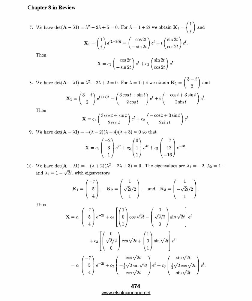
Chapter 8 in Review
7. We have det(A - AI) = A2 - 2A + 5 = 0. For A = 1 + 2i we obtain Ki = and
X, = ,(l+2£)f _ / co»2t\e, + ,\ — sin 21J \ cos 2t )
Then / cos 21 \ f ( sin 21\ f X = ci . n ef +C2 n I e . V — sin 21 j V cos 21 J
S. We have det(A — AI) = A2 — 2A + 2 = 0. For A = 1 + i we obtain Ki = ( j and
Xl = ( 3 ; ! , e (U i)t _ /^cosf-i-sint^ e + 1 cos t + 3 sin t \ 2 sin t )
Then\ 2 cos t
( 3 cost ~ sint \ t ( — cost + 3 sint \ . = Cl( 2 cosf ) ' - + <*{ 2 sm« ) e '
e*.
9. We have det(A — AI) = —(A — 2)(A — 4)(A + 3) = 0 so that/ —2 \ / 0 \ / 7 \
X = ci 3i y
e2i + C2 1VI /
e4t + C3 12 V- 1 6 /
-3 t
.0 . Wc have det(A — AI) = —(A + 2)(A2 — 2A + 3) = 0. The eigenvalues are Ai = —2 , A2 = 1 and A2 = 1 — y/2i, with eigenvectors
/ —7 \ ( 1 ^ / 1 \K i = 5 , k 2 = V2i/2 , and K3 = -y /2 i / 2
v 4 J 1 J V 1 /i hus
/ —7 \ /1\( ° ^X = ci 5 e~2t + c2 0 cos a/2t — y/2/2 sin V21v 4 ) UJ \ 0 )
d
+ C3
/ —7\
54 /
/ ° \ V2/2
LV 0 /cos V21 +
( 1 \0
wsin \ [ 2 t
e 2t + c2
cos \f2t \ -|\/2 sin \ / 2 t
cos y/21 )e -I- C3
/ sin V2t \ 5 \/2 cos y/2 t
\ sin \ / 2i /c*.
474www.elsolucionario.net

Chapter 8 in Review
We have
Thenx c = CI( ; V + c 2( * y ‘.
$ = ' e2t Aeu n tA t
-21 -4e—2t'-41 f ’
andU = j $ _1F dt = J ' 2e~2i - 64£e_2t \ _ / 15e~2t + 32te -‘it, '
16£e' -44 ,-4t 4ie-4tso that
11 + 16£' - 1-4 £
We have
Then
and
so that
/ 2 cos t \ . ( 2 sin t \ ,X c = o, . , e‘ + c2 M .V — sin £ j V cos £ )
2 cos £ 2 sin £' — sin £ cos £ e‘, = | cos £ — sin £ \ _
.5 sin £ cos £ /
/■ -i /• / cos £ — see £ \ / sin £ — In j sec £ + tan £|u = y ™ = / ( sin( ) * = ( cost
—2 cos £ In | sec£ -f- tan£| \ f -1 + sin£ln | sec£ + tan£| /
We have
Then
and
( cos £ + sin t \ ( sin £ — cos i 'X(: = Cll 0 v + C'2 \ o • +\ 2 cos £ / \ 2 sin £
$ cos £ + sin £ sin £ — cos £' 2 cos £ 2 sin £ S - 1 =
sin t cos £ — sin £' — cos £ \ cos £ + | sin £,
[ 1 1 t , / / s s in £ — i cos £ + i csc £ \U = / * " 1F i t= i \ 2. 2. *J \ — 5 sm t — A cos £ + A csc £ /cos £ — | sin £ + 5 In | csc £ — cot £|'
cos £ — | sin £ + | In | csc £ — cot £ j .
475www.elsolucionario.net

Chapter 8 in Review
?o thatX« = $ U = sin t
1 In I csc t — cottl. sin t + cos f /14. We have
ThenX c = c, j )e2t + c2
- 1te2t +
$ =e2t te2t + e2t\ _x / - t e 2t - t e 2t - e 2t
_ e2* _ te2t j * * = 1 g- 2f e- 2t
-aidU - i
f - l \ , / i t 2 — t dt = ‘ - tso that
15. (a) Letting1
K =( h \
h\ h )
we note that (A — 21)K = 0 implies that 3fci + 3k2 + 3% = 0, so k-\ = —(k'2 + k ). Ch k‘2. = 0 . A'3 — 1 and then k2 — 1 , fc.3 = 0 we get
/ —1 \ / - 1 \Ki = 0
1 /and K2 =
respectively. Thus,
X i =/ - 1 \
0
1 /e2t and Xo
1
0 )
/ - 1 \1
0 /,.2t
are two solutions.(b) From det(A — AI) = A2(3 — A) = 0 wc see that Ai = 3, and 0 is an eigenvalue of mu/
/ * i \two. Letting
K = k2\ h l
476www.elsolucionario.net
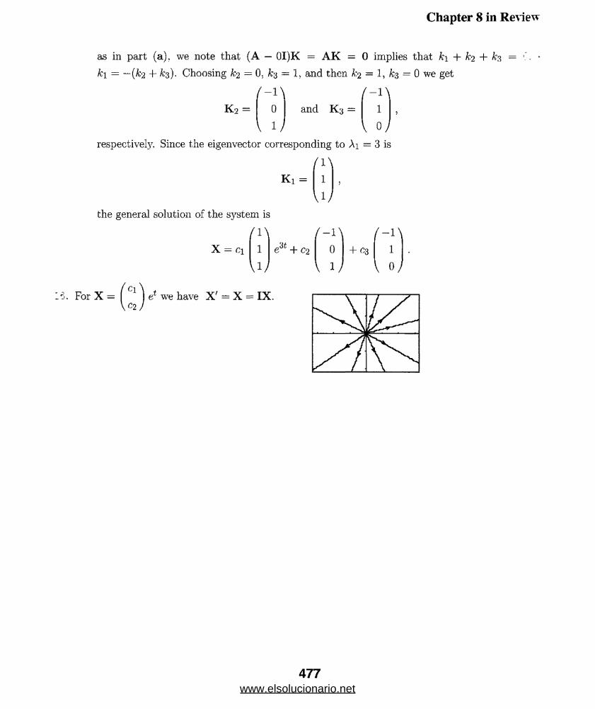
Chapter 8 in Review
as in part (a), we note that (A — 0I)K = AK = 0 implies that k\ + k2. + ks — ki = —(k'2 + ks). Choosing k-2 = 0, k;$ — 1, and then k2 = 1, kz — 0 we get
/ - 1 \ / —1 \K , -- 0
1 /and K3 1
0 /respectively. Since the eigenvector corresponding to Ai = 3 is
n \Ki =
the general solution of the system is/ 1 \
X = ci 1
V I )
est + C2
1
V I/
i - l \ 0
1 /+ .3
/ —1 \ 1
V o y
Cl16. For X = I ^ J ef we have X' = X = IX.
477www.elsolucionario.net

9 Numerical Solutions of Ordinary Differential Equations
Euler Methods and Error Analysis
3.
sr 1! p i—1
Xn1.00 5 .0000
1 .10 3 .9900
1.20 3 .2546
1.30 2 .7236
1.40 2 .3451
; 1.50 2 .0801
fc=0.1
Xn y n0.00 0.00000.10 0 .1005
0.20 0 .2030
0 .30 0 .3098
0 .40 0 .4234
0 .50 0 .5470
h =0.05
yn1.00 5 .0000
1 .05 4 .4475
1. 10 3 .9763
1 .15 3 .5751
1.20 3 .2342
1 .25 2 .9452
1 .30 2 .7009
1 .35 2 .4952
1 .40 2 .3226
1 .45 2 .1786
1 .50 2 .0592
ft—0.05
Xn0.00 0.00000 .05 0 .0501
0.10 0.1004
0 .15 0.1512
0.20 0 .2028
0 .25 0 .2554
0 .30 0 .3095
0 .35 0 .3652
0 .40 0 .4230
0 .45 0 .4832
0 .50 0 .5465
/?.—0.1 h =0.05
Xn yn Xn yn0.00 2.0000 0.00 2.00000.10 1 .6600 0 .05 1.8150
0.20 1 .4172 0.10 1.6571
0 .30 1 .2541 0 .15 1.5237
0 .40 1 .1564 0.20 1.4124
0 .50 1 . 1 12 2 0 .25 1.3212
0 .30 1.2482
0 .35 1 .1916
0 .40 1 .1499
0 .45 1.1217
0 .50 1.1056
h - 0.1 h 0.05
yn Xn yn0.00 1.0000 0.00 1.00000.10 1 . 1 1 1 0 0 .05 1.0526
0.20 1.2515 0.10 1.1113
0 .30 1.4361 0 .15 1.1775
0 .40 1 .6880 0.20 1.2526
0 .50 2 .0488 0 .25 1.3388
0 .30 1.4387
0 .35 1.5556
0 .40 1.6939
0 .45 1.8598
0 .50 2.0619
478
www.elsolucionario.net
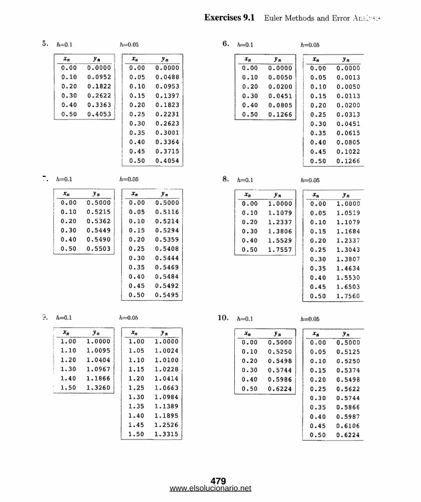
Exercises 9.1 Euler Methods and Error Ati£.L"=;
o. h=o.l fv= 0.05 6 . h= 0.1 ft=0.05
Xn0 .00
0 . 1 00.200.30
0.40
0.50
A=0.1
ft=0.1
yn0 .0000
0.0952
0.1822
0.2622
0.3363
0.4053
y»0.00 0.5000
0.10 0.5215
0.20 0.5362
0.30 0.5449
0.40 0.5490
0.50 0.5503
y«1.00 1.0000
1.10 1.0095
1.20 1.0404
1.30 1.0967
1.40 1.1866
1.50 1.3260
yn0.00 0.00000.05 0.0488
0.10 0.0953
0.15 0.1397
0.20 0.1823
0.25 0.2231
0.30 0.2623
0.35 0.3001
0.40 0.3364
0.45 0.3715
0.50 0.4054
/i=0.05
Xn yn0.00 0.5000
0.05 0.5116
0.10 0.5214
0.15 0.5294
0.20 0.5359
0.25 0.5408
0.30 0.5444
0.35 0.5469
0.40 0.5484
0.45 0.5492
0.50 0.5495
fc=0.05
Xn y n1.00 1.00001.05 1.0024
1.10 1.0100
1.15 1.0228
1.20 1.0414
1.25 1.0663
1.30 1.0984
1.35 1.1389
1.40 1.1895
1.45 1.2526
1.50 1.3315
10.
Xn yn
0.00 0.0000
0.10 0.0050
0.20 0.0200
0.30 0.0451
0.40 0.0805
0.50 0.1266
h=0.1
Xa yn
0.00 1.0000
0.10 1.1079
0.20 1.2337
0.30 1.3806
0.40 1.5529
0.50 1.7557
fc=0.1
Xtt yn
0.00 0.5000
0.10 0.5250
0.20 0.5498
0.30 0.5744
0 .40 0.5986
0.50 0.6224
xn y n
oo9O
0 . 0000
0.05 0.0013
0.10 0.0050
0.15 0.0113
0.20 0.0200
0.25 0.0313
0.30 0.0451
0.35 0.0615
0.40 0.0805
0.45 0.1022
0.50 0.1266
/t—0.05
Xn y n0 .00 1.0000
0.05 1.0519
0.10 1.1079
0.15 1.1684
0.20 1.2337
0.25 1.3043
0.30 1.3807
0.35 1.4634
0.40 1.5530
0.45 1.6503
0.50 1.7560
/i=0.05
Xn y n0 .00 0.5000
0.05 0.5125
0.10 0.5250
0 .15 0.5374
0.20 0.5498
0.25 0.5622
0.30 0.5744
0.35 0.5866
0.40 0.5987
0.45 0.6106
0.50 0.6224
479www.elsolucionario.net

Exercises 9.1 Euler Methods and Error Analysis
11. To obtain the analytic solution use the substitution u = x + y — 1. The resulting differential equat: in u(x) will be separable.
fi.=0.05h=0.1
Xn y tt ActualValue0 .0 0
0.100.20
0 .30
0 .40
0 .50
2.00002 .1 2 2 02.3049
2.5858
3.0378
3.8254
2.0000
2 .1230
2 .3085
2 .5958
3 .0650
3 .9082
Xn ynActualValue
0.00 2.0000 2.00000 .05 2.0553 2 .1230
0.10 2.1228 2 .3085
0 .15 2 .2056 2 .5958
0-20 2 .3075 3 .0650
0 .25 2 .4342 3 .9082
0 .30 2 .5931 2 .5958
0 .35 2 .7953 2 .7997
0 .40 3 .0574 3 .0650
0 .45 3 .4057 3 .4189
0 .50 3 .8840 3 .9082
12. (a) y (b)2015
105
1.1 1.2 1.3 1.4
Xn Euler Im p. Euler
1.00 1.0000 1.00001.10 1.2000 1.2469
1.20 1.4938 1.6430
1.30 1.9711 2.4042
1.40 2.9060 4.5085
13. (a) Using Euler’s method we obtain ;t/(0.1) m y\ = 1.2.(b) Using y" — 4e2x we see that the local truncation error is
y“(c) % = (° ' 1)2 = 0 .02e2c.2 " 2
Since e2x is an increasing function, e2c < e2 01) = e0-2 for 0 < c < 0.1. Thus an upper for the local truncation error is 0.02e0,2 = 0.0244.
(c) Since ?/(0.1) — e02 = 1.2214, the actual error is y(0 .1) — y\ = 0.0214, which is less than 1
(d) Using Euler’s method with h — 0.0-5 we obtain 2/(0 .1) ~ y-2 — 1.21.(e) The error in (d) is 1.2214 — 1.21 = 0.0114. With global truncation error 0(h ), when T:;
size is halved we expect the error for h = 0.05 to be one-half the error when h = 0.1. Con/0.0114 with 0.0214 we see that this is the case.
14. (a) Using the improved Euler’s method we obtain y(0 .1) « y\ = 1.22 .(b) Using y"' = 8e2a: we see that the local truncation error is
y"'(c) y = 8e2f: = 0.001333e2c.
480www.elsolucionario.net
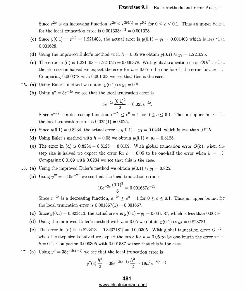
Since e2;r is an increasing function, e2c < e2(G1) = e0,2 for 0 < c < 0.1. Thus an upper bn for the local truncation error is 0.001333f;(l'2 = 0.001628.
(c) Since y(0.1) = e0,2 = 1.221403, the actual error is y(0 .1) — y\ = 0.001403 which is less0.001628.
(d) Using the improved Euler's method with h = 0.05 we obtain ?/(0.1) ~ y-2 = 1.221025.(e) The error in (d) is 1.221403 — 1.221025 = 0.000378. With global truncation error 0(h~ . v
the step size is halved we expect the error for h = 0.05 to be one-fourth the error for h = Comparing 0.000378 with 0.001403 we see that this is the case.
(a) Using Euler’s method we obtain |/(0.1) ~ y\ = 0.8.(b) Using y" = 5e-2x we see that the local truncation error is
5e-2 c = o.025e_2c.Since e~2x is a decreasing function, e~2r < e° — 1 for 0 < c < 0.1. Thus an upper bounc the local truncation error is 0.025(1) = 0.025.
(c) Since y(0.1) = 0.8234, the actual error is y(0.1) — y\ = 0.0234, which is less than 0.025.(d) Using Euler’s method with h = 0.05 wc obtain y(0.1) rs yi = 0.8125.(e) The error in (d) is 0.8234 — 0.8125 = 0.0109. With global truncation error 0(h ), whe::
step size is halved we expect the error for h — 0.05 to be one-half the error when h = Comparing 0.0109 with 0.0234 wc see that this is the case.
(a) Using the improved Euler's method we obtain y(0 .1) ~ y\ — 0.825.(b) Using y'" = — 10e-2z we see that the local truncation error is
l 0e- 2c (0^ = o.001667e_2c.6
Since e""2x is a decreasing function, e-2c < e° = 1 for 0 < c < 0.1. Thus an upper bouiK the local truncation error is 0.001667(1) = 0.001667.
(c) Since y(0.1) = 0.823413, the actual error is y(0.1) —y i = 0.001587, which is less than 0.001(d) Using the improved Euler’s method with h, — 0.05 we obtain y(0.1) ~ y-2 = 0.823781.(e) The error in (d) is |0.823413 — 0.82371811 = 0.000305. With global truncation error O
when the step size is halved we expect, the error for h = 0.05 to be one-fourth the error v h = 0.1. Comparing 0.000305 with 0.001587 we see that this is the case.
(a) Using y" = wc sec that the local truncation error is/ ( , . ) ^ = S f e - 3'0- 1 ) % = 19
Exercises 9.1 Euler Methods and Error Anal;.
481www.elsolucionario.net
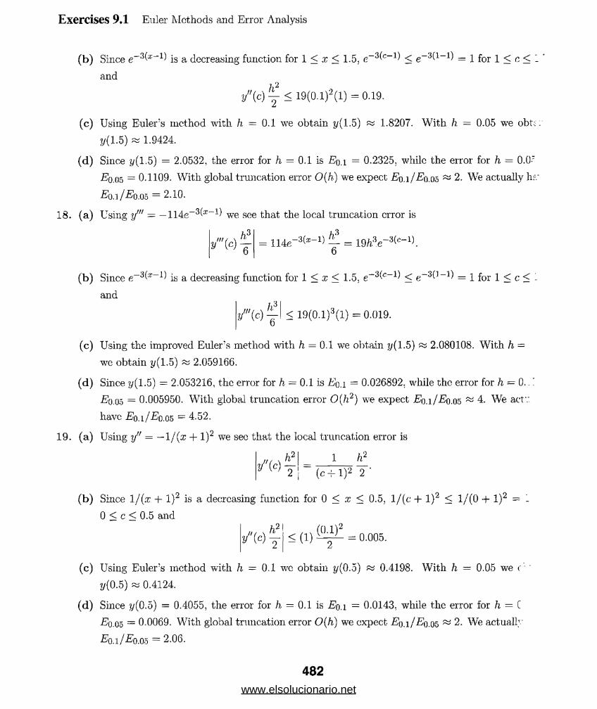
Exercises 9.1 Euler Methods and Error Analysis
(b) Since e ^ is a decreasing function for 1 < x < 1.5, e 3<-c ^ < e ^ = 1 for 1 < c < 1
and/ ( c ) y < 1 9 ( 0 . 1 ) 2( l ) = 0.19.
(c) Using Euler’s method with h = 0.1 we obtain y(1.5) « 1.8207. With h = 0.05 we obt;: 2/(1.5) « 1.9424.
(d) Since y(1.5) = 2.0532, the error for h = 0.1 is Eq\ = 0.2325, while the error for h = 0 .0” Eo.(m — 0.1109. With global truncation error 0(h) we expect EJq.i/E q.Oo ~ 2 . We actually h?/Eqa/E q.qo = 2 .10.
18. (a) Using ym — —114e_3^ -1 we see that the local truncation error ish3 = u r ' i - - 1) - =
6
(b) Since e ^ is a decreasing function for 1 < x < 1.5. e 3'c ^ < e ^ = 1 for 1 < c < and
y'"(c) y < 19(0.1)3(1) = 0.019.(c) Using the improved Euler’s method with h = 0.1 we obtain y( 1.5) ~ 2.080108. With h =
we obtain y(1.5) ~ 2.059166.(d) Since f/(1.5) - 2.053216, the error for h = 0.1 is £?o.i = 0.026892. while the error for h = 0..'
■o.05 = 0.005950. With global truncation error 0(h2) we expect jBo.i/^o.os ~ 4. We actv. have Eq.i/Eq.os = 4.52.
19. (a) Using y" = — l j{x + l )2 we see that the local truncation error is"< \ h2\ y (c)-d =
i h2
2 I (c -r I)'2 2
(b) Since l / (x + l )2 is a decreasing function for 0 < x < 0.5, l/(c + l )2 < 1 /(0 + 1)2 _0 < c < 0.5 and
h2\y"(c) ^ < (1) = 0.005.
(c) Using Euler’s method with h — 0.1 we obtain y(0.o) ~ 0.4198. With h = 0.05 we c y{0.5) w 0.4124.
(d) Since y(0.5) = 0.4055, the error for h = 0.1 is Eo.i — 0.0143, while the error for h — C Eo.oo = 0.0069. With global truncation error 0(h) we expect ^o.i/^o.os ~ 2. We actually Eq.i /EQ'Qo = 2.06.
482
www.elsolucionario.net
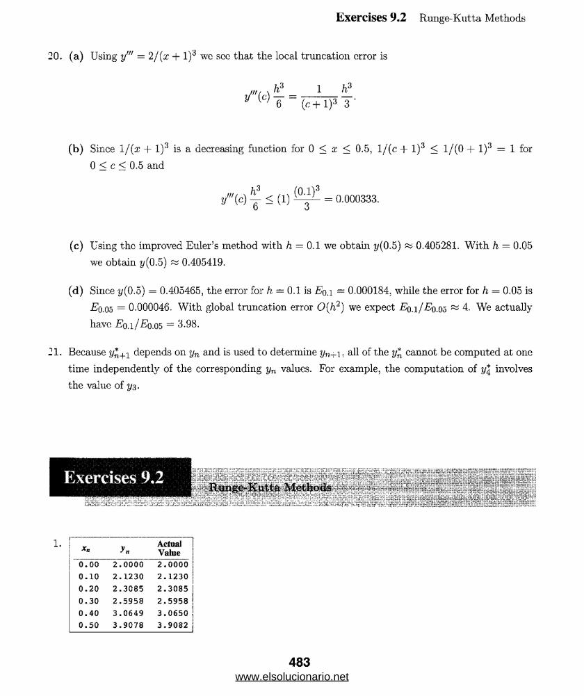
Exercises 9.2 Runge-Kutta Methods
h3 i yfi fit / \ 11 L n
y “ ( c + 1)3 T ‘
20. (a) Using y'" = 2/(x + 1) we see that the local truncation error is
(b) Since l / (x + l )3 is a decreasing function for 0 < x < 0.5, l / ( c + 1) 3 < 1 /(0 + l )3 = 1 for0 < c < 0.5 and
/' ( c ) ^ < (1) = 0.000333.0 o
(c) Using the improved Euler’s method with h = 0.1 we obtain t/(0.5) « 0.405281. With h = 0.05 we obtain 2/(0 .5) « 0.405419.
(d) Since y(0.5) = 0.405465. the error for h — 0.1 is E$,\ — 0.000184. while the error for h = 0.05 is ■Eb.05 = 0.000046. With global truncation error 0(h2) we expect Eq^/Eq.os ~ 4. We actually have Eq,i/Eq.q5 = 3.98.
21. Because j/*+1 depends on yn and is used to determine yn+1. all of the y* cannot be computed at one time independently of the corresponding yn values. For example, the computation of t/| involves the value of y%.
1. yn ActualValue
0*00 2.0000 2.0000
0.10 2.1230 2.1230
0.20 2.3085 2.3085
0.30 2.5958 2.5958
0.40 3.0649 3.0650
0.50 3.9078 3.9082
483www.elsolucionario.net
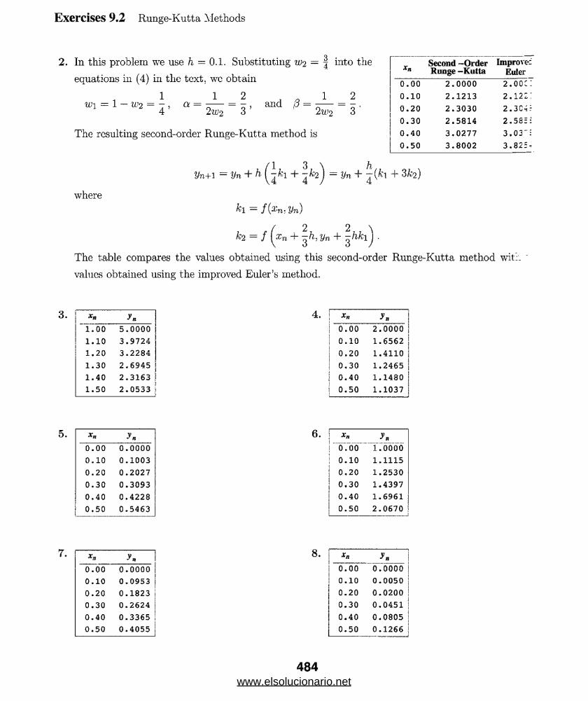
Exercises 9.2 Runge-Kutta Methods
2 . In this problem we use h = 0.1. Substituting W2 — | into theequations in (4) in the text, wc obtain
2
3 5
, 1 1wi = 1 - W2 = - , a = - — 4 2u'2 and .3 = 2w223
The resulting second-order Runge-Kutta method is
Xn Second -Order Runge -Kutta
Improve:
Euler
0.00 2.0000 2 . 00c :
0.10 2.1213 2 . 122:
0 .20 2.3030 2.3043
0.30 2.5814 2.583:
0.40 3.0277 3.03~:
0.50 3.8002 3.825.
Un+1 — Un + h + ^ ’2) — I-1” 4 ^ 1 ' '2)where
k l — f {'Xn . Vn)
X r ,
2 2 y-n + ^hkih = fThe table compares the values obtained using this second-order Runge-Kutta method wit:, values obtained using the improved Euler’s method.
*n !
0 0 5.0000 |
1.10 3.9724 |
1.20 3.2284
1.30 2.6945 |
1.40 2.3163 [
1.50 2.0533 j
Xny■
0.00 2.0000 10 0 1.6562 |
0.20 1.4110 j
0.30 1.2465 j00
1.1480 [
0.50 1.1037 |
5. x„ J*
OOO
0.0000
0.10 0.1003
0.20 0.2027
0.30 0.3093
0.40 0.4228
0.50 0.5463
XnO o r."oooo
0 ♦ h-* 0 1.1115
0.20 1.2530
0.30 1.4397
0.40 1.6961
0.50 2.0670
7. Xn
0.00 0.0000
0.10 0.0953
0.20 0.1823
0.30 0.2624
0.40 0.3365
0.50 0.4055
yn| 0.00 0.0000
1 0.10 0.0050
1 0.20 0.0200
j 0.30 0.0451
| 0.40 0.0805
| 0.50 0.1266
484www.elsolucionario.net
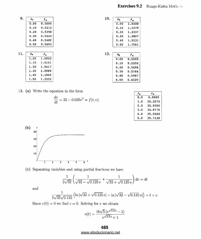
Exercises 9.2 Rimgc-Kutta Methc
Xn yn0 . 0 0 0 . 5 0 0 00 , 1 0 0 . 5 2 1 3
o ro o 0 . 5 3 5 80 . 3 0 0 . 5 4 4 3oo 0 . 5 4 8 20 . 5 0 0 . 5 4 9 3
10.
Xn
1 . 0 0 1 . 0 0 0 01 . 1 0 1 . 0 1 0 11 . 2 0 1 . 0 4 1 71 . 3 0 1 . 0 9 8 91 . 4 0 1 . 1 9 0 51 . 5 0 1 . 3 3 3 3
12.
xn
o o o 1 . 0 0 0 00 . 1 0 1 . 1 0 7 90 . 2 0 1 . 2 3 3 70 . 3 0 1 . 3 8 0 70 . 4 0 1 . 5 5 3 10 . 5 0 1 . 7 5 6 1
Xn ooo 0 . 5 0 0 00 . 1 0 0 . 5 2 5 00 . 2 0 0 . 5 4 9 80 . 3 0 0 . 5 7 4 40 . 4 0 0 . 5 9 8 70 . 5 0 0 . 6 2 2 5
(a) Write the equation in the form dv- = 3 2 - 0.025v* = f(t,v).CL L
(b)
and
*n Vno»o 0 . 0 0 0 01 . 0 2 5 . 2 5 7 02 . 0 3 2 . 9 3 9 03 . 0 3 4 . 9 7 7 04 . 0 3 5 . 5 5 0 05 . 0 3 5 . 7 1 3 0
(c) Separating variables and using partial fractions we have
2^32 ( \ / 3 2 - + V32 + \ / 0 2 f v ) dV ~ <U
2 ^ ^ /0 1 2 5 ^ ,V/^ + v/^ t '1 _ ln 1 - V 0l25v |) = t + Since v(0) = 0 wc find c = 0. Solving for v we obtain
v(t) = 16 v/5 (■ 1)e\/&2t + i
www.elsolucionario.net

Exercises 9.2 Runge-Kutta Methods
and u(5) ~ 35.7678. Alternatively, tho solution can be expressed as
(a) rj t (days) | 1 2 3 4 5
j A (observed) j 2.78 13.53 36.30 47.50 49.40
j A (iapproximated ) | 1.93 12.50 36.46 47.23 \D O O
lb) From the graph wc estimate A(l) « 1 .68 , A(2) ~ 13.2, A(3) ^ 36.8, A(A) « 46.9, and A(5) ss 48.9.
c) Let a = 2.128 and 6 — 0.0432. Separating variables we obtaindA
A{a - pA)P
= dt
- ( - + a a — pA1
dA ~ dt
a [In A — 1ii(q' — &A)\ = t + c
In a - p AA
— a(t + c)_ e<x(t+c)
ThusA(t) =
a - PAA = aea{l+c) - pAea(t+c)
' l+ P e a^ } A = a ^ {t+c\
<yea(t+c') a a1 + /?ea(*+c) P -I- p + e ~ a c c ~ a t '
From A(0) = 0.24 we obtain0.24 = a
p + e~ac
486www.elsolucionario.net
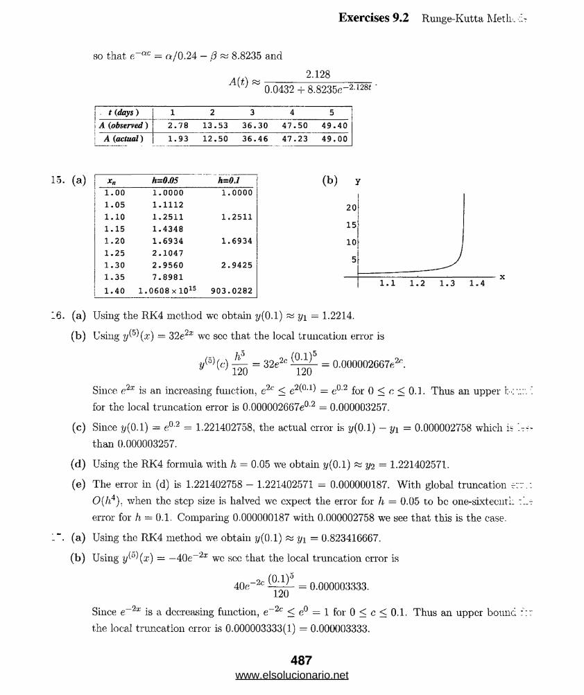
Exercises 9.2 Runge-Kutta. Meth.
A{t)so that e ac = a /0.24 — /? ^ 8.8235 and
2.1280.0432 + 8.8235c-2-128*
] t {days ) 1 2 3 4 5| A (observed) 2 . 7 8 1 3 . 5 3 3 6 . 3 0 4 7 . 5 0 4 9 . 4 0| A (actual) 1 . 9 3 1 2 . 5 0 3 6 . 4 6 4 7 . 2 3 4 9 . 0 0
(a) h~0.05 h=0.1
1.00
1 . 0 5 1 . 1 0 1 . 1 5 1.20 1 . 2 5 1 . 3 0 1 . 3 5 1 . 4 0
1.0000
1 . 1 1 1 2 1 . 2 5 1 1 1 . 4 3 4 8 1 . 6 9 3 4 2 . 1 0 4 7 2 . 9 5 6 0 7 . 8 9 8 1
1 . 0 6 0 8 x 10¹⁵
1.0000
1 . 2 5 1 1
1 . 6 9 3 4
2 . 9 4 2 5
9 0 3 . 0 2 8 2
(b) y
(a) Using the RI<4 method wc obtain 2/(0 .1) ~ yi = 1.2214.(b) Using t/ 5) (.r) — 32e2x wc see that the local truncation error is
„<5>w y W 120 ~ J 120 = 0.000002667^.
Since e2x is an increasing function, e2c < e2(0-1) — e0,2 for 0 < c < 0.1. Thus an upper b>:' for the local truncation error is 0.000002667e°‘2 = 0.000003257.
(c) Since f/(0.1) = e0,2 = 1.221402758, the actual error is 2/(0 .1) — y\ = 0.000002758 which is than 0.000003257.
(d) Using the RK4 formula with h = 0.05 we obtain 2/(0.1) ~ ;</2 = 1.221402571.(e) The error in (d) is 1.221402758 - 1.221402571 = 0.000000187. With global truncation e:
0(h4), when the step size is halved wc expect the error for h = 0.05 to be one-sixteenth error for h = 0.1. Comparing 0.000000187 with 0.000002758 we see that this is the case.
(a) Using the RK4 method we obtain y(0 .1) ~ yi = 0.823416667.(b) Using (a;) — —40e 2x we sec that the local truncation error is
120
Since e 2x is a decreasing function, e 2c < e° = 1 for 0 < c < 0.1. Thus an upper bound the local truncation error is 0.000003333(1) = 0.000003333.
487www.elsolucionario.net
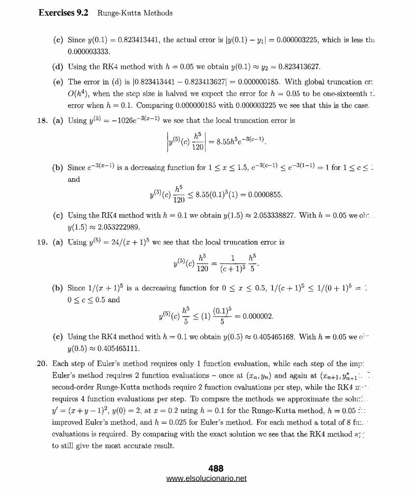
Exercises 9.2 Runge-Kutta Methods
(c) Since y(0 .1) = 0.823413441, the actual error is |y(0.1) — y i \ = 0.000003225, which is less tht.0.000003333.
(d) Using the RK4 method with h ~ 0.05 we obtain y(0 .1) ~ y-2 = 0.823413627.(e) The error in (d) is |0.823413441 — 0.823413627| = 0.000000185. With global truncation cr:
0(/i4), when the step size is halved we expect the error for h = 0.05 to be one-sixteenth i. error when h — 0 .1. Comparing 0.000000185 with 0.000003225 wc see that this is the case.
18. (a) Using y ^ = —1026e~3 ’~1 we see that the local truncation error ish5(c)J K } 120 = 8.55 /?5e ' 3(c_1).
(b) Since e ' x ^ is a decreasing function for 1 < x < 1.5. e 3(-c ^ < e 3^ ^ = 1 for 1 < c < 1
andi / 5\c ) — < 8.55(0.1)5 (1) = 0.0000855.L
(c) Using the RK4 method with h, = 0.1 we obtain y( 1.5) ~ 2.053338827. With h - 0.05 we ol):.. y(1.5) « 2.053222989.
19. (a) Using t/5) = 24/(x + l )5 we see that the local truncation error is(5W \ hb 1 * 5V ^ 120 _ (c + l )5 5 ‘
(b) Since l / (x + l )5 is a decreasing function for 0 < x < 0.5, l/(c + l ) 5 < 1 /(0 + l )5 = 1
0 < c < 0.5 andy(5) (c) ^ < (1) = 0 .000002 .O 0
(c) Using the RK4 method with h — 0.1 wc obtain t/(0.5) ~ 0.405465168. With h = 0.05 we o%‘ y(0.5) « 0.405465111.
20. Each step of Euler’s method requires only 1 function evaluation, while each step of the imp: Euler's method requires 2 function evaluations - once at (xn,yn) and again at (xn+i,j/*+1:. ” second-order Runge-Kutta methods require 2 function evaluations per step, while the RK4 n>'. requires 4 function evaluations per step. To compare the methods we approximate the soluti.. y' — (x + y — l )2, y(0) = 2 . at x — 0.2 using h = 0.1 for the Runge-Kutta method, h = 0.05 ::: improved Euler’s method, and h = 0.025 for Euler’s method. For each method a total of 8 fu:. ' evaluations is required. By comparing with the exact solution wc see that the RK4 method a::; to still give the most accurate result.
488www.elsolucionario.net

Exercises 9.2 Runge-Kutta M
Xn Eulerh=0.O25
Im p. Euler h=0.O5
RK4h-0.1
Actual
0.000 2.0000 2.0000 2.0000 2.0000
0.025 2.0250 2.0263
0,050 2.0526 2.0553 2.0554
0.075 2.0830 2.0875
0.100 2.1165 2.1228 2.1230 2.1230
0.125 2.1535 2.1624
0.150 2.1943 2.2056 2.2061
0.175 2.2395 2.2546 j
0.200 2.2895 2.3075 2.3085 2.3085 j
(a) For y' + y = 10 sin 3x an integrating factor is ex so thatd 5— [exij] = 10e'T sin 3x = > exy = ex sin 3x — 3ex cos 3x + c dx
=r- y — sin 3;e — 3 cos 3x + ce~x. _When x = 0, y = 0. so 0 = — 3 + c and c = 3. The solution is
y = sin 3a: — 3 cos 3x + 3e~x.-5
Using Newton:s method we find that x = 1.5323-5 is the only positive root in [0 , 2].
(b) Using the RK4 method with h = 0.1 we obtain the table of values shown. These values to obtain an interpolating function in Mathematica. The graph of the interpolating fui shown. Using Mathematical root finding capability we see that the only positive root is x = 1.53236.
Xn
0 . 0 0.0000
0 . 1 0 . 1 4 4 00 . 2 0 . 5 4 4 80 . 3 1 . 1 4 0 90 . 4 1 . 8 5 5 90 . 5 2 . 6 0 4 90 . 6 3 . 3 0 1 90 . 7 3 . 8 6 7 500•o 4 . 2 3 5 60 . 9 4 . 3 5 9 31 . 0 4 . 2 1 4 7
Xn 3^1 . 0 4 . 2 1 4 71 . 1 3 . 8 0 3 31 . 2 3 . 1 5 1 31 . 3 2 . 3 0 7 61 . 4 1 . 3 3 9 01 . 5 0 . 3 2 4 31 . 6 - 0 . 6 5 3 01 . 7 - 1 . 5 1 1 700•r*“f - 2 . 1 8 0 91 . 9 - 2 , 6 0 6 12 . 0 - 2 . 7 5 3 9
www.elsolucionario.net
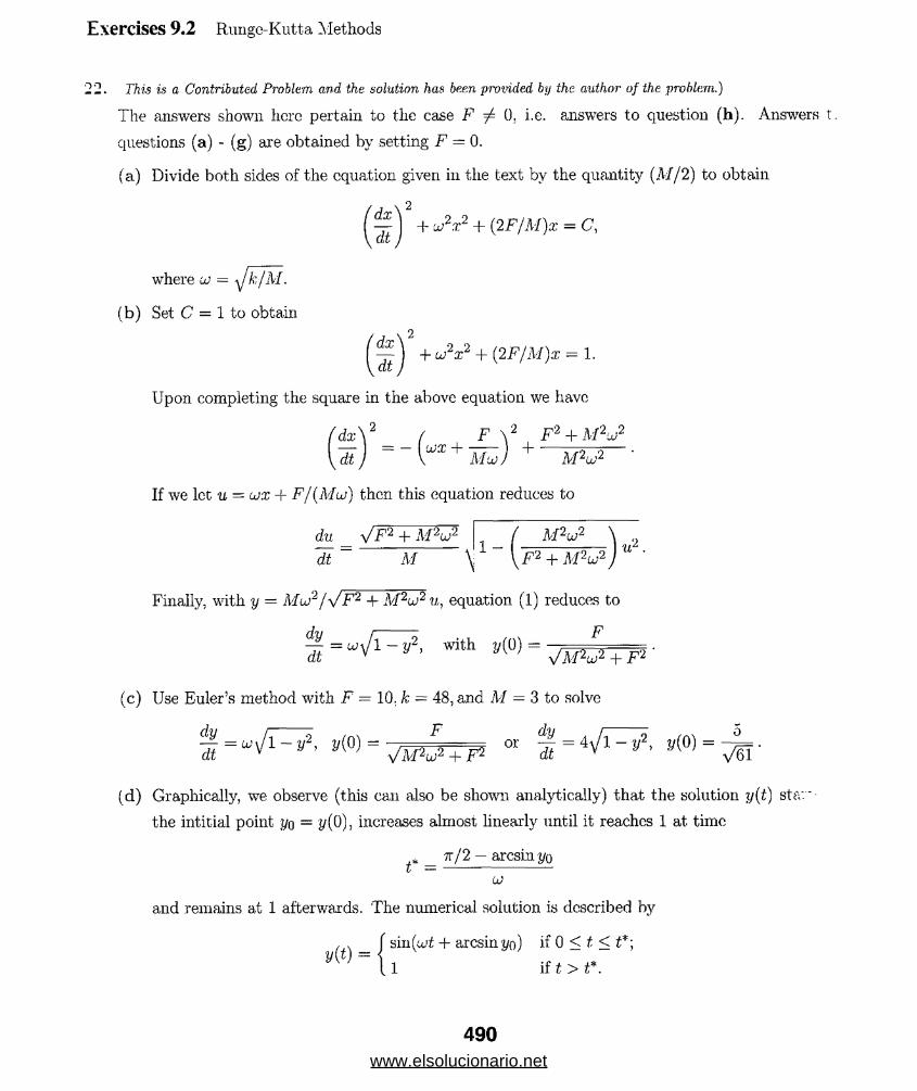
Exercises 9.2 Runge-Kutta Methods
This is a Contributed Problem and the solution has been provided by the author of the problem.)
The answers shown here pertain to the case F (), i.e. answers to question (h). Answers tquestions (a) - (g) are obtained by setting F — 0.(a) Divide both sides of the equation given in the text by the quantity (M /2) to obtain
(d) Graphically, we observe (this can also be shown analytically) that the solution y(t) stav the intitial point yo = increases almost linearly until it reaches 1 at time
* tt / 2 — arcsinyo t — (Jand remains at 1 afterwards. The numerical solution is described hv
where lj = yjk/M.(b) Set C = 1 to obtain
Upon completing the square in the above equation we have
If we let u = ujx Ff (Mu ) then this equation reduces todu V ! i = ~
Finally, with y = MuP/y/F2 + M2u)2u, equation (1) reduces to
(c) Use Euler’s method with F — 10. k = 48, and M = 3 to solve
sin(cot + arcsinyo) if 0 < t < t*;1
490
www.elsolucionario.net
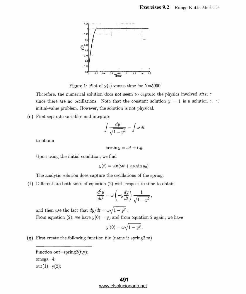
Exercises 9.2 R/unge-Kutta Methc
Figure 1: Plot of y(t) versus time for N=5000Therefore, the numerical solution docs not seem to capture the physics involved after : since there are no oscillations. Note that the constant solution y = 1 is a solution initial-value problem. However, the solution is not physical.
(e) First separate variables and integrateI ■— — = j Lodt J \ / l - y 2 '
to obtainarcsiny = ojt -I- Cq.
Upon using the initial condition, we findy(t) = sin(u;t + arcsin y ).
The analytic solution does capture the oscillations of the spring.(f) Differentiate both sides of equation (2) with respect to time to obtain
d j l dy \ 1
dt2 Vd t) v/i _ y2 !and then use the fact that dy/dt = wy'l — y2 .From equation (2), we have y(Q) = yo and from equation 2 again, we have
y'{0 ) = a;^/l — yg .(g) First create the following function file (name it spring2.m)
function out=spring2 (t ,v);omega=4;out(l)=y(2);
491www.elsolucionario.net

Exercises 9.2 Runge-Kutta Methods
out(2)=-o;2 * 2/(1); out=out?;
then in the Matlab window, type the following commands:
» M = 3; k = 48: a; = Jk/M: F = 10 :» y() = F/yJ(M2£J2 + F2)» 2/1 = w y 1 - 2/0
>> [t, y] = ode45('spring? , [0 ,pz/2], [yo, 2/i] : » plot (t .y(:, 1))
where y\ - dy/dt at t = 0. The resulting plot is shown in figure 2 . The graph is consist:: with the analytical solution y(t) = sin(o>t + arcsinyo) from part (e).
Time
Figure 2 : Plot of y(t) versus time using ODE45
The second-order differential equation has constant coefficients. The analytic solutio:. easily be obtained,
, . VF2 + M 2oj2 ( , , yi , Fx(t) = — — (,»cos^ ) + tr sm(a,t)J " ■
492www.elsolucionario.net

Exercises 9.3 Multistep Methods
Multistep Methodsr V . •; ' " ; ... • •: :: /•
the tables in this section £:ABM‘> stands for' Adams-Bashforth-Moulton.
1 . Writing the differential equation in the form y1 — y = x — 1 we see that an integrating factor ise - J dx _ g0
-ie-'y] = (x - 1)<T*
andy = ec(—xe~x + c) = — x + cex.
From y(0) = 1 we find c = 1, so the solution of the initial-value problem is y = —x + ex. Actual values of the analytic solution above are compared with the approximated values in the table.
Xn Actualoo 1 .00000000 1.00000000 i n i t . cond.0 .2 1.02140000 1.02140276 RK40 . 4 1.09181796 1.09182470 RK40 .6 1.22210646 1.22211880 RK4COo 1 .42552788 1.42554093 ABM
2 . The following program is written in Mathematica. It uses the Adams-Bashforth-Moulton method to approximate the solution of the initial-value problem y' = x + y — 1 , y(0 ) = 1, on the interval [0 , 1].
Clear[f, x, y, h, a, b, yO];f[x_, y_]:= x + y - 1 ; (* define the differential equation *)h = 0 .2 ; (* set the step size *)a = 0 ; y 0 = l ; b = l; (* set the initial condition and the interval *)f[x, y] (* display the DE *)Clear[kl, k2, k3, k4, x, y, u, v] x = u[0 ] — a; y = v[0] = yO; n = 0 ;W hile[x < a + 3h, (* use RK4 to compute the first 3 values after y(0) *)
n = n 4- 1;
493
www.elsolucionario.net

Exercises 9.3 Multistep Methods
(* use Adams-Bashforth-Moulton *)
k l = f[x, y];k2 = f[x + h /2 , y + h k l / 2 ]; k3 = f[x + h / 2 , y + h k2/2]; k4 = f[x + h, y + h k3]: x = x + h;y = y + (h /6 )(k l -f 2k2 + 2k3 + k4); u[n] = x; v[n] = y];
W hile [x < b,p3 = f[u[n - 3], v[n - 3]]; p2 = f[u[n - 2], v[n - 2 ]]; p i = f[u[n - 1], v[n - 1]]; pO = f[u[n], v[n]];pred = y + (h /24)(55p0 - 59pl + 37p2 - 9p3): (* predictor * x = x + h; p4 = f[x, pred];y = y 4 - (h/24)(9p4 + 19p0 - 5p l + p2); (* corrector *n = n + 1 ; u[n] = x; v[n] = y]
(*display the table *)TableForm[Prepend[Table[{u[n], v[n]}, {n, 0, (b-a)/h}], {"x(n)", "y(n)"}
3. The first predictor is y% — 0.73318477.xn J n0 .0 1.00000000 i n i t . cond.0-2 0.73280000 RK40.4 0.64608032 RK40.6 0.65851653 RK40 .8 0.72319464 ABM
4. The first prcdictor is y\ = 1.21092217.Xn yn ! i* ....... 50 .0 2.00000000 ! i n i t . cond. 1i0 .2 1.41120000 j RK40 .4 1.14830848 RK4 |0 .6 1.10390600 ! RK4 |0 .8 1.20486982 j ABM !
494
www.elsolucionario.net
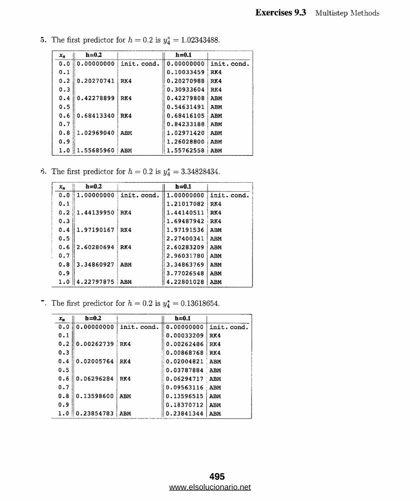
Exercises 9.3 Multistep Methods
5. The first predictor for h = 0.2 is y% = 1.02343488.Xn h=0.2 h=Q.l0 .0 0.00000000 i n i t . cond. 0.00000000 i n i t . cond.0 .1 0.10033459 RK40.2 0.20270741 RK4 0.20270988 RK40 .3 0.30933604 RK40.4 0.42278899 RK4 0.42279808 ABM0 .5 0.54631491 ABM0.6 0.68413340 RK4 0.68416105 ABM0.7 0.84233188 ABM00o 1.02969040 ABM 1.02971420 ABM0 .9 1.26028800 ABM1.0 1.55685960 ABM 1.55762558 ABM
6 . The first predictor for h — 0.2 is y% — 3.34828434.i h=0.2A- .............. h=0.1oo 1.00000000 i n i t . cond. 1.00000000 i n i t . cond.
i o . i !s 1 .21017082 RK40 .2 1.44139950 RK4 1.44140511 RK40 .3 | 1 .69487942 j RK4
j 0 .4 | 1 .97190167 RK4 1.97191536 ABMino I 2 .27400341 ABM0.6 [2.60280694 RK4 2.60283209 ABM
! 0 .7 S! 2 .96031780 ABM00o | 3 . 3 4 8 6 0 9 2 7 ABM 3.34863769 ABM0 .9 ij 3.77026548 ABM1.0 | 4 . 2 2 7 9 7 8 7 5 ABM 4.22801028 ABM
The first predictor for h = 0.2 is y l = 0.13618654.Xn cr 1! O: h=0.1
o.
o 0 .00000000 i n i t . cond . 0.00000000 i n i t . cond.
0 .1 0.00033209 RK40.2 0.00262739 RK4 0.00262486 RK40.3 0.00868768 RK40.4 0.02005764 RK4 0.02004821 ABM
0 .5 0.03787884 !ABM
0.6 0.06296284 RK4 0.06294717 ;ABM
0.7 0.09563116 ABM
COo 0.13598600 ABM 0.13596515 ABM
0.9 0.18370712 ABM
1.0 0.23854783 ABM 0.23841344 ABM
495www.elsolucionario.net
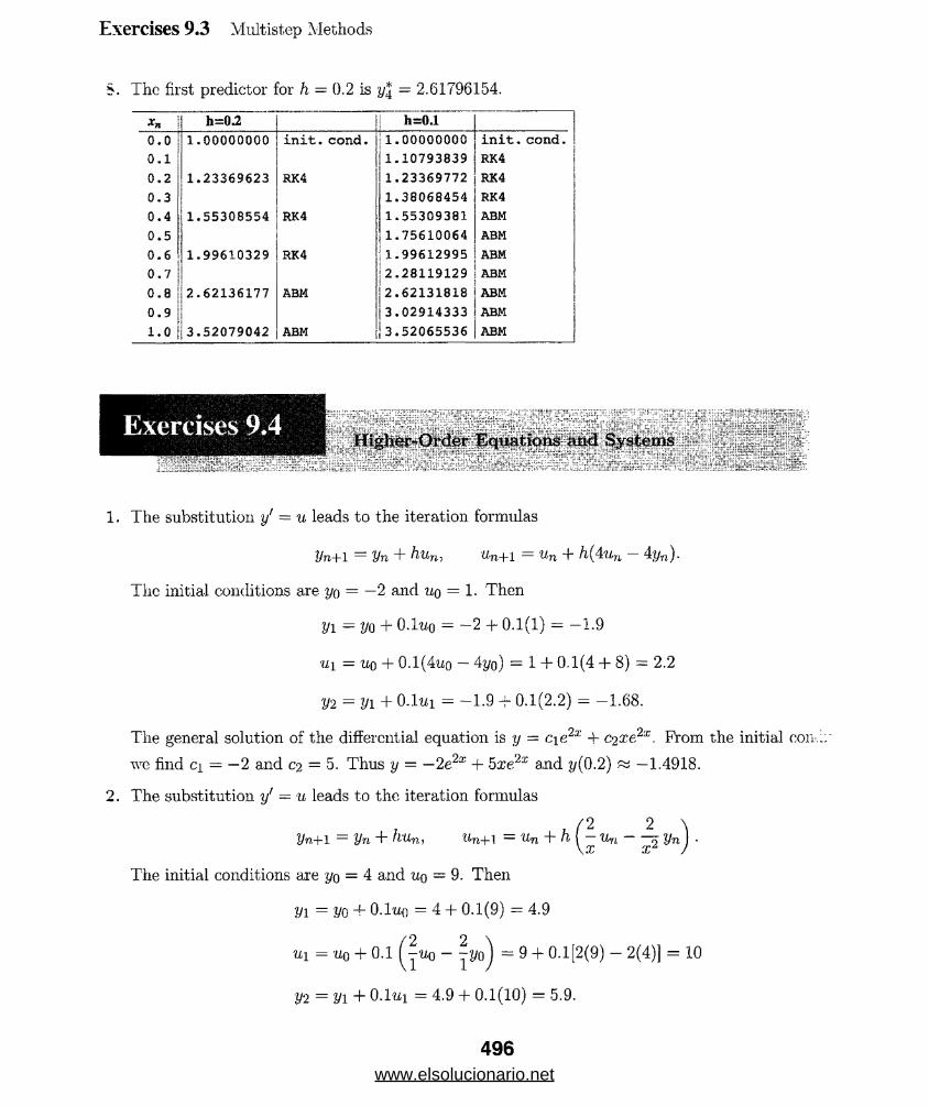
Exercises 9.3 Multistep Methods
S. The first predictor for h — 0.2 is y\ — 2.61796154.Xn h-0.2 h=0.10 .0 1.00000000 i n i t . cond. 1 .00000000 i n i t . cond.0-1 1.10793839 RK40 .2 1*23369623 RK4 1.23369772 RK40.3 1.38068454 RK40-4 1.55308554 RK4 1.55309381 ABM0.5 1.75610064 ABM0.6 1.99610329 RK4 1.99612995 ABM0.7 2 .28119129 ABM0.8 2 .62136177 ABM 2.62131818 ABM0.9 3.02914333 ABM1.0 3 .52079042 ABM 3.52065536 ABM
1 . The substitution y' = u leads to the iteration formulasUn+ 1 = Vn h t t j t, u n + 1 = Un h ( 4 u n 4 y n ).
The initial conditions are yo = —2 and uo = 1. ThenPi - I/O + O.lwo = - 2 + 0.1(1) = -1 .9ui = uq + 0.1(4tto — 4yo) = 1 + 0.1(4 + 8 ) = 2.2
V2 = yi + O.ltti = -1 .9 -f- 0 .1(2 .2) = - 1.68 .The general solution of the differential equation is y = c\e?x + C2xe?x. Prom the initial con.:: we find ci = —2 and C2 = 5. Thus y = —2e2a? + 5xe2x and ?y(0.2) « —1.4918.
2 . The substitution y' — u leads to the iteration formulasVn+ 1 = Vn "t" hum ^n+ 1 = Un + h Un Vn j •
The initial conditions are yo = 4 and uq = 9. ThenS/i = 2/0 + 0.1-uo = 4 + 0.1(9) - 4.9ui = uo + 0.1 Q wo — ^ 0) = 9 + 0.1[2(9) — 2(4)] = 10V‘2 = Vi + O.ltti = 4.9 + 0.1(10) = 5.9.
496www.elsolucionario.net
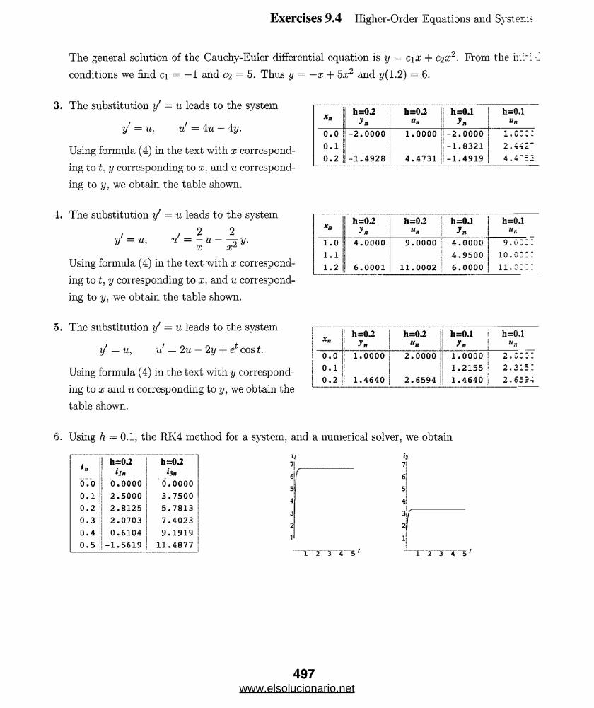
Exercises 9.4 Higher-Order Equations and System-
The general solution of the Cauchy-Eulor differential equation is y = C\x + c^x2. From the ir.i'i conditions we find ci = — 1 and 02 = 5. Thus y — —x + 5x2 and 7/(1.2) — 6 .
3. The substitution y' = u leads to the systemy ~ u. u' = 4u — 4y.
Using formula (4) in the text with x corresponding to t. y corresponding to x. and u corresponding to y, we obtain the table shown.
1Xn
h-0.2 h=0.2Un
h=0.1
y nh=0.1
0O
-2.0000 1.0000 \ -2.0000 i . o c : :
0 .1 -1.8321 2.442*'
0 . 2 - 1 . 4 9 2 8 4*4731 1 - 1 . 4 9 1 9 4 . 4 ~ 3 5
4. The substitution y' = u leads to the system, 2 2
y = u - u — - u — T y. x x.Using formula (4) in the text- with x corresponding to t. y corresponding to x. and u corresponding to y. we obtain the table shown.
Xn h—0«2y n h-02Un j h=0.1yn h=CM1.0 4 .0000 9 .0000 j 4 . 0 0 0 0 9 . 0 : : :1 .1 1 4 .9500 1 0 . oc::1 .2 6.0001 11.0002 | 6 .0000 11. 0c::
5. The substitution 1/ = u leads to the systemy' = u, u' = 2u — 2y -j- ef‘ cos t.
Using formula (4) in the text with y corresponding to x and u corresponding to y. we obtain the table shown.
I xn h=0*2 h—0.2 h=0.1 h=0.1
“a
0 .0 1.0000 2.0000 1.0000 ; 2 . c : :•:
0.1 1-2155 ! 2 .31 3 :0 .2 1.4640 2.6594 1 .4640 : 2 .6554
6 . Using h =0.1, the RK4 method for a system, and a numerical solver, we obtain4 h=0.2 h=0.2tn tin hnd.o 0.0000 0 . 0 0 0 00 . 1 2 .5000 3 .75000 . 2 j 2 .8125 5 .78130 . 3 i 2 .0703 7.40230 . 4 j 0 .6104 9.19190 . 5 ; -1 .5 6 1 9 11.4877
*27!ej5}4f
' 1...2 ... 3...4... 5 1 1 2 3 4 5 J
497www.elsolucionario.net

Exercises 9.4 Higher-Order Equations and Systems
tnh=0-2
Xn
h=0.2 h=0.1 h=0.1
oo 6 . 0 0 0 0 2 . 0 0 0 0 6 . 0 0 0 0 2 . 0 0 0 00 . 1 7 . 0 7 3 1 2 . 6 5 2 40 . 2 8 * 3055 3 . 4 1 9 9 8 . 3 0 5 5 3 *4199
x,y
tnh-0 .2
Xn
h=0 2y n
h~0.1Xn
h=0,ly noo 1*0000 1 . 0 0 0 0 1 . 0 0 0 0 1 . 0 0 0 0
0 . 1 1 . 4 0 0 6 1 . 8 9 6 30 . 2 2 . 0 7 8 5 3 . 3 3 8 2 2 . 0 8 4 5 3 . 3 5 0 2
tnh=0a IXji h = 0 2y» h=0.1 !
Xn |h=0.1
0.0 - 3 . 0 0 0 0 5 . 0 0 0 0 - 3 . 0 0 0 0 | 5 . 0 0 0 00.1 | - 3 . 4 7 9 0 ] 4 . 6 7 0 70.2 - 3 . 9 1 2 3 | 4 . 2 8 5 7 - 3 . 9 1 2 3 | 4 . 2 8 5 7
498www.elsolucionario.net
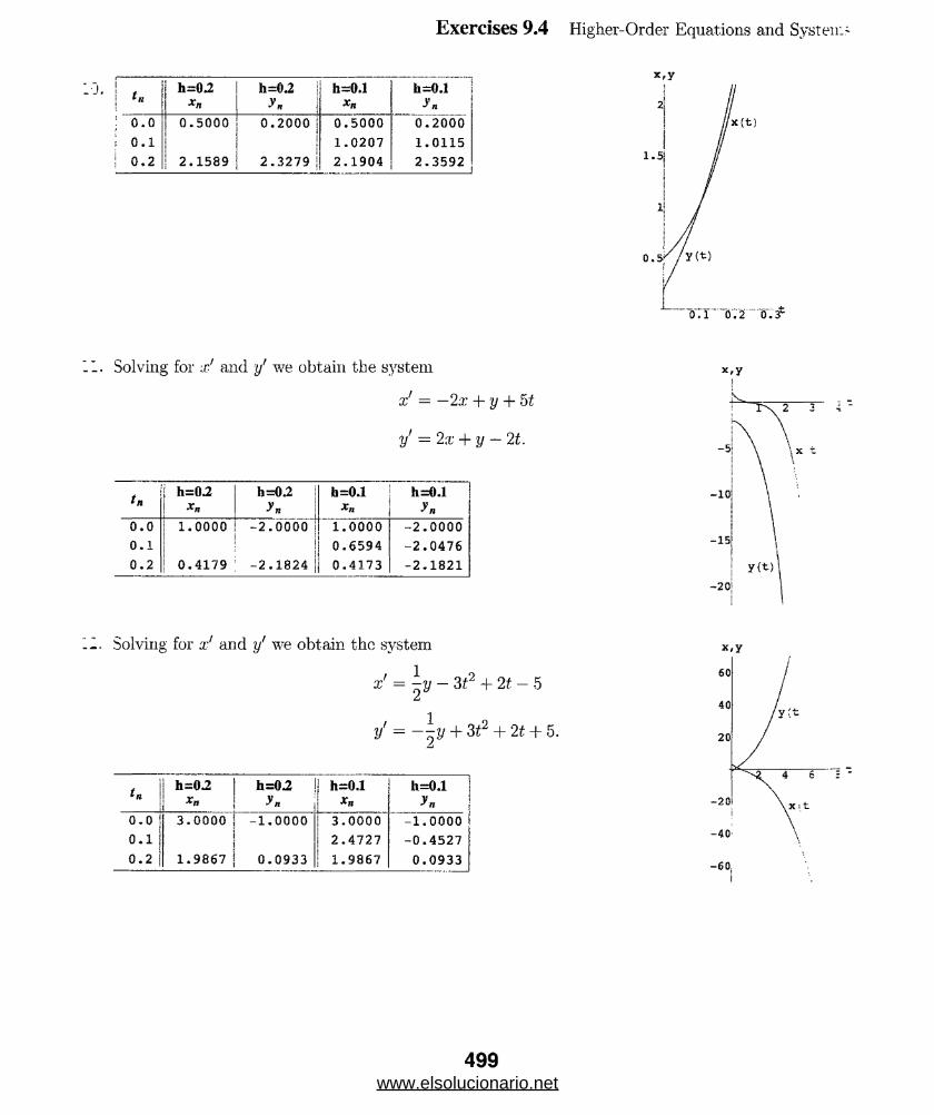
Exercises 9.4 Higher-Order Equations and Systems
j h=0^I xni
h-0.2y n
h“0.1Xn
h=0.1
oo I 0.5000 0.2000 0 .5000 0 .2000i o.i 1 .0207 1.0115! 0*2 2 .1589 2 .3279 2 .1904 2.3592
II. Solving for xf and y' we obtain the systemx' = —2x + y + hty' — 2x + y — 2t.
tnh=0.2
Xn
h=0,2 fa-0.1Xn
h=0.10 .0 1 . 0 0 0 0 - 2 . 0 0 0 0 1 . 0 0 0 0 - 2 . 0 0 0 00 .1 0.6594 - 2 . 0 4 7 60 .2 0.4179 I - 2 . 1 8 2 4 0 .4173 -2 .1 8 2 1
II. Solving for x1 and y' we obtain the system/ 1 9x = - y — 31 + 2t — 5
y = jV H" 3t2 + 2t. + 5.
oToo .i0-2
h - 0 2Xn
h=0 2 \yn h-0.1Xn
h=0.1y»3.0000 -1.0000 3 .0000 -1.0000
2 .4727 -0 .4 5 2 71.9867 0.0933 1.9867 0 .0933
x'y
x,y
-60j
499www.elsolucionario.net
Exercises 9.5 Second-Order Boundary-Value Problems
Second-Order Boundary-Vetlue Problems
1 . We identify P{x) = 0. Q{x) = 9. f(x) = 0. and h — (2 — 0)/4 = 0.5. Then the finite differenc equation is
Vi+i + 0-25yi -r yi-1 - 0 .The solution of the corresponding linear system gives
0 . 0 0 . 5 1 . 0 1 . 5 2 . 04 . 0 0 0 0 - 5 . 6 7 7 4 - 2 . 5 8 0 7 6 . 3 2 2 6 1 . 0 0 0 0
2 . We identify P(x) ~ 0, Q(x) = —1. f(x) = x2. and h = (1 — 0)/4 = 0.25. Then the finite differed, equation is
y-t+i _ 2.0625?/* + tji-i = 0.0625a;?.The solution of the corresponding linear system givesX 0 . 0 0 0 . 2 5 oino 0 . 7 5 1.00
y 0 , 0 0 0 0 - 0 . 0 1 7 2 - 0 . 0 3 1 6 - 0 . 0 3 2 4 0.0000
3. We identify P{x) = 2 , Q(x) = 1, f(x) — 5.x, and h = (1 — 0)/5 = 0 .2 . Then the finite differ-::. equation is
1.2-t/i+i — 1.96 yi + 0.8tji-i = 0.04(5xj).
The solution of the corresponding linear system gives0 . 0 0 . 2 0 . 4 0 . 6 0 . 8 1 . 0
0 . 0 0 0 0 - 0 . 2 2 5 9 - 0 . 3 3 5 6 - 0 . 3 3 0 8 - 0 . 2 1 6 7 0 . 0 0 0 0
4. We identify P(x) = —10. Q(x) = 25, f(x) = 1. and h = (1 — 0)/5 = 0.2. Then the finite diffc: -. equation is
—yi + 2yj_i =0.04.
The solution of the corresponding linear system gives0 . 0 0 . 2 0 . 4 0 . 6 0 . 8 1 . 0
1 . 0 0 0 0 1 . 9 6 0 0 3 . 8 8 0 0 7 . 7 2 0 0 1 5 . 4 0 0 0 0 . 0 0 0 0
5. We identify P(x) = —4, Q(x) = 4, f(x) = (1 + x)e2x, and h = (1 — 0)/6 = 0.1667. Then the r difference equation is
0.6667y,;+i - 1.8889^ + 1.3333y*_i = 0.2778(1 + a*)e2a*.
500www.elsolucionario.net
Exercises 9.5 Second-Order Boundary-Value Problems
The solution of the corresponding linear system givesX 0.0000 0 . 1 6 6 7 0 . 3 3 3 3 0 .5 0 0 0 0 . 6 6 6 7 0 . 8 3 3 3 1-0000
Y 3 . 0 0 0 0 3*3751 3 .6 3 0 6 3 .6 4 4 8 3 . 2 3 5 5 2 . 1 4 1 1 0.0000
Wc identify P(x) = 5. Q(x) — 0, f(x) = 4v/x . and h = (2 — l ) /6 — 0.1667. Then the finite difference equation is
1.4167^+1 - 2Vi + O.o833j/i_i = 0 .2 7 7 8 (4 ^ ).The solution of the corresponding linear system givesX 1 .0 0 0 0 1 .1 6 6 7 1 .3 3 3 3 1 . 5 0 0 0 1 .6 6 6 7 1 .8 3 3 3 2 . 0 0 0 0y 1 , 0 0 0 0 - 0 . 5 9 1 8 - 1 . 1 6 2 6 - 1 . 3 0 7 0 - 1 . 2 7 0 4 - 1 . 1 5 4 1 - 1 . 0 0 0 0
We identify P(x) = 3/x. Q(x) = 3/a:2, f (x ) = 0, and h — (2 — l ) /8 = 0.125. Then the finite difference equation is
„ 0.1875 \ ( n 0.0469\ (, 0.1875 \1 + ~ i r ) m + i + 1 - 2 ~ w ~ ) V i + ( W _ 1 _
The solution of the corresponding linear system givesX 1 . 0 0 0 1 .1 2 5 1 . 2 5 0 1 * 375 1 .5 0 0 1 . 6 2 5 1 . 7 5 0 1 . 8 7 5 2 . 0 0 0Y 5 . 0 0 0 0 3 . 8 8 4 2 2 . 9 6 4 0 2 . 2 0 6 4 1 .5 8 2 6 1 .0 6 8 1 0 . 6 4 3 0 0 . 2 9 1 3 0 . 0 0 0 0
We identify P(x) = —1/x, Q(x) = x 2, f(x) = lnx/x2, and h = (2 — l ) /8 = 0.125. Then the finitedifference equation is
, 0.0625 \ / „ 0.0156 \ / 0.0625\1 ------) Vi+1 + I - 2 + 2— l yi + (1 + — ) yi-1 = 0.0156 In a:,;.i i / y J V X'l /
The solution of the corresponding linear system givesX 1 . 0 0 0 1 . 1 2 5 1 . 2 5 0 1 .3 7 5 1 .5 0 0 1 . 6 2 5 1 .7 5 0 1 . 8 7 5 2 . 0 0 0y 0 . 0 0 0 0 - 0 . 1 9 8 8 - 0 . 4 1 6 8 - 0 . 6 5 1 0 - 0 . 8 9 9 2 - 1 . 1 5 9 4 - 1 . 4 3 0 4 - 1 . 7 1 0 9 - 2 . 0 0 0 0
We identify P(x) = 1 — x, Q(x) = x, f(x) = x, and h = (1 — 0)/10 = 0.1. Then the finite difference equation is
[1 + 0.05(1 - xi)]y^i + [-2 + 0.0l3i]sfi + [1 - 0.05(1 - a*)]w-1 = O.Olar*.The solution of the corresponding linear system gives
0 . 0 0 . 1 0 . 2 0 . 3 0 . 4 0 . 5 0 . 6 ] 0 .0 0 0 0 0 . 2 6 6 0 0 .5 0 9 7 0 .7 3 5 7 0 .9 4 7 1 1 .1 4 6 5 1 . 3 3 5 3 |
i 0 . 7 0 . 8 0 . 9 1 . 0 j 1 .5 1 4 9 1 .6 8 5 5 1 .8 4 7 4 2 . 0 0 0 0
We identify P(x) — x, Q(x) — 1, /(a:) = x. and h = (1 — 0)/10 = 0.1. Then the finite difference equation is
(1 + 0.05a;7;)t/j+i — 1.99?/; + (1 — 0.05;r.,)t/t_i = 0.01x4.
501www.elsolucionario.net
Exercises 9.5 Second-Order Boundary-Value Problems
The solution of the corresponding linear system givesx 0 . 0 0 . 1 0 . 2 0 . 3 0 . 4 0 . 5 0 . 6 j y I 1 .0 0 0 0 0 . 8 9 2 9 0 . 7 7 8 9 0 . 6 6 1 5 0 .5 4 4 0 0 .4 2 9 6 0 . 3 2 1 6 ;
j 0 . 7 0 . 8 0 . 9 1 . 0 I 0 .2 2 2 5 0 .1 3 4 7 0 .0 6 0 1 0 . 0 0 0 0
11 . We identify P(x) = 0. Q(x) = —4, f(x) -- 0. and h = (1 — 0 )/8 = 0.125. Then the finite differe
12 . We identify P(r) = 2jr. Q(r) = 0, f(r) = 0 . and h = (4 — l ) /6 — 0.5. Then the finite differ- equation is
is the same as equation (8 ) in the text. The equations are the same because the derivation based only on the differential equation, not the boundary conditions. If we allow i to : from 0 to n — 1 we obtain n equations in the n + 1 unknowns y-i , yo. yi, . . . , yn- \ . Si1.:: is one of the given boundary conditions, it is not an unknown.
(b) Identifying yo = y{0), y_i = y(0 — h), and y\ = y(0 + h) we have from equation (5) in tlv
equation is1 — 2.0625yi -r }ji-\ — 0 .
The solution of the corresponding linear system givesX 0 . 0 0 0 0 . 1 2 5 0 . 2 5 0 0 . 3 7 5 0 . 5 0 0 0 . 6 2 5 0 . 7 5 0 0 . 8 7 5 1 . 0 0 0 y j 0 . 0 0 0 0 0 .3 4 9 2 0 . 7 2 0 2 1 .1 3 6 3 1 .6 2 3 3 2 . 2 1 1 8 2 . 9 3 8 6 3 . 8 4 9 0 5 . 0 0 0 0
The solution of the corresponding linear system givesr 1 . 0 1 . 5 2 . 0 2 . 5 3 . 0 3 . 5 4 . 0u 5 0 .0 0 0 0 - 7 2 ; 2 2 2 2 8 3 . 3 3 3 3 9 0 . 0 0 0 0 - 9 4 . 4 4 4 4 - 9 7 > 6 1 9 0 1 0 0 .0 0 0 0
13. (a) The difference equation
The difference equation corresponding to i = 0.
www.elsolucionario.net

Chapter 9 in Review
or2yi + (-2 + h2Qo)yo = h2f o + 2h - PQ.
Alternatively, we may simply add the equation y\ — y-i = 2h, to the list of n difference equ; obtaining n + 1 equations in the n - f 1 unknowns y - i . yo,2/1 > • • • > ?M-i-
(c) Using n = 5 we obtain0.0 0 .2 0 .4 0 .6 0 . 8 1 .0
-2 .2755 -2 .0755 -1 .8589 -1 .6126 -1 .3275 -1.0000
Using h = 0.1 and, after shooting a few times, y'(0) = 0.43535 we obtain the following tabi-> the RK4 method.
0 .0 0 . 1 0 .2 0 .3 0 .4 0 .5 0 .6 j1.00000 1.04561 1.09492 1.14714 1.20131 1.25633 1.31096 1
0 .7 0.8 0 .9 1 . 0« 1.36392 1.41388 1.45962 1.50003
Chapter 9 in Review n> s'j|rpc. P'<-~..........., c-
Eulerh=0.1
Eulerh=0.05
m p. Euler h=0.1
Im p. Euler h 30.05
RK4h=0,l
RK4h “ 0.05
1.00 2.0000 2.0000 2.0000 i 2.0000 2.0000 2.0000
1.05 2.0693 2.0735 2,0736
1.10 2.1386 2.1469 2.1549 2.1554 2.1556 2.1556
1.15 2.2328 2.2459 2.2462
1.20 2.3097 2.3272 2.3439 2.3450 2.3454 2.3454
1.25 2.4299 2.4527 2.4532
1.30 2.5136 2.5409 2.5672 2.5689 2.5695 2.5695
1.35 2.6604 2.6937 2.6944
1.40 2.7504 i 2.7883 2.8246 2.8269 2.8278 2.8278
1.45 2.9245 2.9686 2.9696
1.50 3.0201 3.0690 3.1157 3.1187 3.1197 3.1197 !
503www.elsolucionario.net
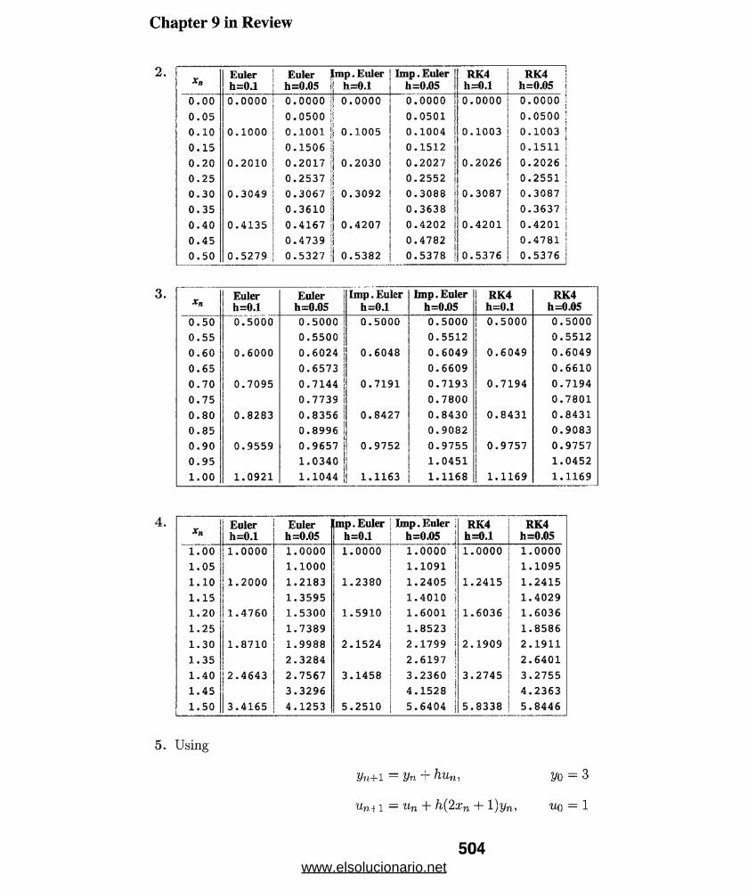
Chapter 9 in Review
Xn Eulerh-0.1
Euler Im p. Eulerh=0.05 l| h~0.1..... h........
Im p . Euler h=O.05
RK4h-0.1 n
&
8*
0 .00 0.0000 0.0000 I 0.0000 0.0000 0.0000 0.0000
0.05 0.0500 II 0.0501 0.0500
0.10 0.1000 0.1001 II 0.1005 0.1004 0.1003 0.1003 j
0 .15 0.1506 | 0.1512 0.1511
0.20 0.2010 0.2017 | 0.2030 0.2027 0.2026 0.2026
0.25 0.2537 | 0.2552 1 0.2551
0.30 0.3049 0.3067 | 0.3092 0.3088 0.3087 0.3087
0.35 0.3610 )l 0.3638 ! 0.3637
0.40 0.4135 0.4167 |j 0.4207 0.4202 0.4201 0.4201
0.45 0.4739 1 0.4782 0.4781
0.50 0.5279 0.5327 | 0.5382 0.5378 0.5376 0.5376
xnEulerh=0.1
Eulerh=0.O5
Im p . Euler
h-0.1
Im p . Euler
h=0.05RK4h=0.1
RK4h=0,05
0.50 0.5000 0.5000 0.5000 0.5000 0.5000 0.5000
0.55 0.5500 0.5512 0.5512
0.60 0.6000 0.6024 0.6048 0.6049 0.6049 0.6049
0.65 0.6573 0.6609 0.6610
0.70 0.7095 0.7144 0.7191 0.7193 0.7194 0.7194
0.75 0.7739 0.7800 0.7801o00o
0.8283 0.8356 0.8427 0.8430 0.8431 0.8431
0.85 0.8996 0.9082 0.9083
o o 0.9559 0.9657 0.9752 0.9755 0.9757 0.9757
0.95 1.0340 1.0451 1.0452
1 . 0 0 1.0921 1,1044 1.1163 1.1168 1.1169 1.1169
Eulerh=0*l
Eulerh~0.05
m p. Euler
h=0.1
Im p. Euler
h=0.05i| RK4! b=0.1st
RK4h=0.05
1.00 1.0000 1.0000 1.0000 1,0000 il 1.0000 1,0000
1.05 1.1000 1.1091 i| 1.1095
1.10 1.2000 1.2183 1.2380 1.2405 |j 1.2415 1.2415
1.15 1.3595 1.4010 1.4029
1.20 1.4760 1.5300 1.5910 1.6001 i| 1.6036 1.6036
1.25 1.7389 1.8523 Ij 1.8586
1.30 1.8710 1.9988 2.1524 2.1799 l| 2.1909<1 2,1911
1.35 2.3284 2.6197u
2.6401
1.40 2.4643 2.7567 3.1458 3.2360 : 3,2745•i 3,2755
1.45 3.3296 4.1528i
4.2363
1.50 3.4165 4.1253 5.2510 5.6404 || 5.8338 5.8446
5. UsingVn+ 1 = 'Un-T-hun, 2/0 = 3Un I 1 — Un + h(2xn 1) Un' UQ = 1
504www.elsolucionario.net
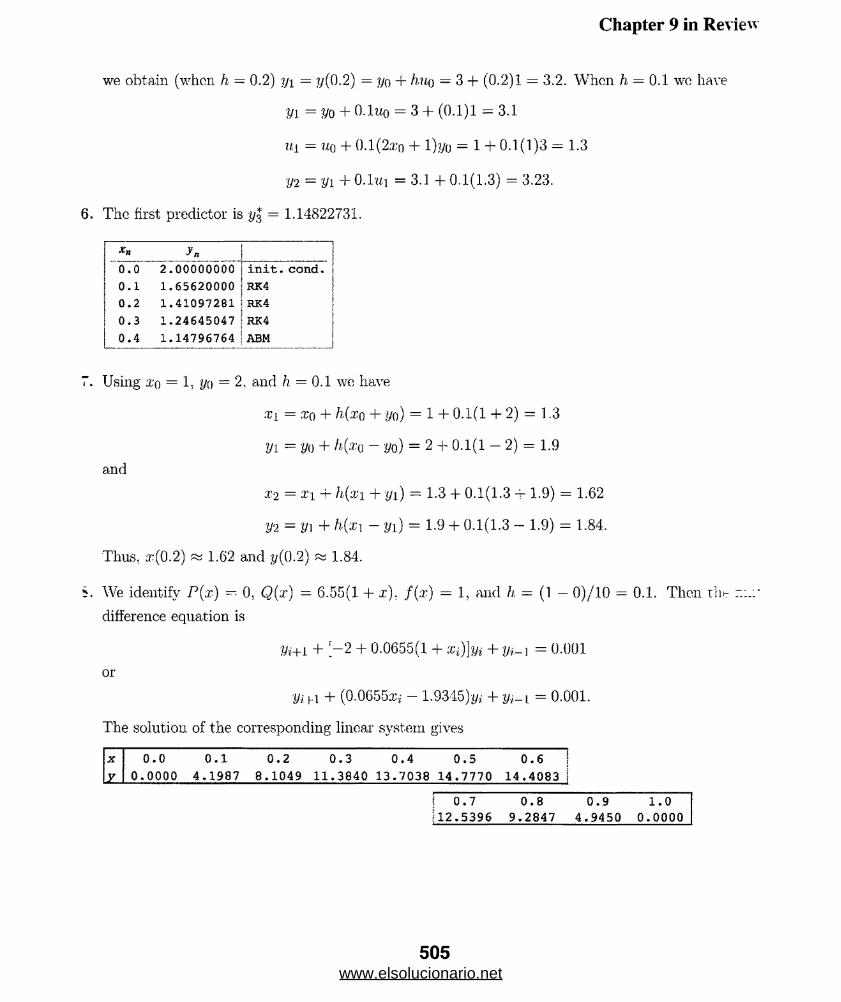
Chapter 9 in Review
we obtain (when h - 0.2) y\ = y(0.2) = yo + hv,Q — 3 + (0.2)1 = 3.2. When h = 0.1 we haveVi = Vo + O.ltio = 3 + (0.1)1 = 3.1ui = u0 + 0.1 (2.1:0 + 1)2/0 = 1 + 0.1(1)3 = 1.3y2 - y i +0.1ui = 3.1 + 0.1(1.3) = 3.23.
6. The first predictor is = 1.14822731.x n yn
\\
0! i
2 . 0 0 0 0 0 0 0 0 i n i t . cond. |0 .1 1.65620000 RK4 |0 .2 1.41097281 RK4 |0 .3 1.24645047 RK4 |0 .4 1.14796764 ABM |
7. Using rro = 1. yo = 2 . and h = 0.1 we have,ti = .to + h(x,Q + yo) = 1 + 0.1(1 + 2) = 1.3 Vi = yo + h{x0 - yo) = 2 + 0.1(1 - 2) = 1.9
andx2 = x1 + h(x! + yi) = 1.3 + 0.1(1.3 + 1.9) = 1.62 V i = y\ + h{x 1 - yi) = 1.9 + 0.1(1.3 - 1.9) = 1.84.
Thus, x(0.2) « 1.62 and ;f/(0 .2) « 1.84.S. We identify P(x) — 0, Q(x) = 6.55(1. + x). f(x) = 1, and h = (1 — 0)/10 = 0.1. Then thfr ~ ■
difference equation isyi+l + [-2 + 0.0655(1 + Xi)]yi + yi- 1 = 0.001
or■yi hi + (0.0655:i',; - 1.9345)y/ + y,- \ = 0.001.
The solution of the corresponding linear system gives x 0T0 oTi 0T2 0T3 0T4 0T5 oTi jy I 0.0000 4.1987 8.1049 11.3840 13.7038 14.7770 14.4083 1
i 0T7 oTs oTi TToj12.5396 9.2847 4.9450 0.0000
505www.elsolucionario.net