solution of coupled acoustic-elastic wave propagation ... · solution of coupled acoustic-elastic...

Solution of Coupled Acoustic-Elastic Wave Propagation Problems with

Anelastic Attenuation Using Automatic

P. J. Matuszyk, L. F. Demkowicz, C. Torres-Verdinby

ICES REPORT 11-03

January 2011

The Institute for Computational Engineering and SciencesThe University of Texas at AustinAustin, Texas 78712

Reference: P. J. Matuszyk, L. F. Demkowicz, C. Torres-Verdin, "Solution of Coupled Acoustic-Elastic Wave Propagation Problems with Anelastic Attenuation Using Automatic hp-Adaptivity", ICES REPORT 11-03, The Institutefor Computational Engineering and Sciences, The University of Texas at Austin, January 2011.

Solution of Coupled Acoustic-Elastic Wave Propagation

Problems with Anelastic Attenuation Using Automatic

hp-Adaptivity

P. J. Matuszyka,b, L. F. Demkowiczc, C. Torres-Verdina

aDepartment of Petroleum And Geosystems Engineering, The University of Texas atAustin, TX 78712, USA

bDepartment of Applied Computer Science and Modeling, Faculty of Metals Engineeringand Industrial Computer Science, AGH – University of Science and Technology, Krakow,

PolandcInstitute for Computational Engineering and Sciences (ICES), The University of Texas

at Austin, TX 78712, USA

Abstract

The paper presents a hp-adaptive Finite Element method for a class of cou-pled acoustics/anelasticity problems with application to modeling of sonictools in the borehole environment. A careful verification of the methodologyand solutions of non-trivial examples involving fast and slow formations withsoft layers are presented.

Keywords: acoustic logging, borehole acoustics, wave propagation, linearelasticity, coupled problems, hp-adaptive finite elements

1. Introduction

Motivation. Accurate numerical simulations of borehole sonic tools enhancethe understanding of sonic logs in complicated scenarios (logging while drilling,multilayer formations, casings, mud invasions etc.) and help to improve thetechnology and design of new generations of sonic tools. The simulations fallinto the class of coupled problems: borehole fluid is modeled with inviscidacoustics, tool and casing with elasticity, and the models for the formationrange from relatively simple isotropic elasticity through anisotropic elasticityand viscoelasticity to various poroelasticity theories.

The presented work is a continuation of [1]. The method of choice isthe hp Finite Element (FE) method with a fully automatic hp-adaptivity

based on the two-grid paradigm described in [2, 3]. Speaking mathemati-cally, the hp method delivers exponential convergence (error vs. number ofdegrees-of-freedom, CPU time or memory use), for both regular and irregu-lar solutions. The problem under study encounters many of such irregulari-ties. At junctions of three or more different materials, stresses are singular,material anisotropies and the use of Perfectly Matched Layer (PML) leadsto internal and boundaries layers. Foremost, however, the solution “lives”mostly along the borehole/formation in presence of strong interface waves. Ifleft unresolved, these irregularities pollute the solution at points of interest(receivers) and result in completely erroneous numerical solutions.

A common misconception is the claim that infinite stresses are non-physical and, therefore, need not be resolved. Although the simplified modelsbased on various elasticity models do result in non-physical infinite stresses(in reality, the material undergoes a plastic deformation), they capture cor-rectly the energy distribution and provide meaningful models away from thesingularities. Leaving the singularities unresolved distorts the energy distri-bution and produces wrong results away from them. Of course, only a com-parison with experiments allows for an ultimate validation of the models andthis is exactly the direction in which we are heading. Assessing the validity ofthe model requires high fidelity discretizations with negligible discretizationerror and this is where the use of hp methods is critical.

The presented contribution focuses on extending the hp technology tomultiphysics coupled problems. A starting point for the new hp code devel-oped in the course of this project, has been a new hp framework [4] designedfor coupled problems (different physics in different subdomains) and sup-porting the hp-adaptivity for elements forming the exact sequence, i.e. H1-,H(curl)-, H(div)- and L2-conforming elements. In this project, only the clas-sical H1-conforming elements are used. Extending the hp adaptive algorithmto coupled problems requires additional modifications of the algorithm whichare discussed in this contribution.

The main goal of this paper is however to demonstrate a maturity ofthe hp-technology in context of non-academic, industrial-strength examples.This includes a careful verification of the code and solution of a number ofnon-trivial examples non-accessible with other methods.

Mathematics of coupled problems. The subjects of acoustics and elasticity areclassical. Discussion on linear problems of elastic structures coupled to fluidsin bounded and unbounded domains can be found e.g. in [5]. The subject of

2

interest relates to the category of problems involving a compact perturbationof a continuous linear operator see, e.g., [6]. In [7] and [8], Demkowicz hasstudied the asymptotic stability of those problems and has shown how itrelates to the convergence of the eigenvalues of the discrete problem to thoseof the continuous problem. A rigorous mathematical analysis for a relatedclass of coupled problems can be found in [9]. The analysis does not includethe PML truncation. Numerical analysis of the coupled acoustics/elasticityproblem with the PML truncation is an open problem.

Simulations of sonic tools. The numerical modeling of the wave propagationproblem in the complex borehole environment has nearly 40-years history.First, the semi-analytical methods were used, where the solution of nonlineardispersion equations and numerical integration in the complex domain wereobtained numerically. Almost all of these models assumed radial symmetry.Such approach was documented in various technical papers but the mostcomprehensive exposition of this topic can be find in [10, 11, 12].

The finite difference time domain technique (FDTD) is currently the mostoften used method for numerical simulation of sonic logging measurements.At the beginning, the simple model of the open borehole surrounded by ho-mogenous or horizontally layered formation was developed [13]. The FDTDapproach was successfully applied to the monopole acoustic logging in bore-holes with washouts and damaged zones [14]. Later on, a 2D-FDTD methodfor simulation axisymmetric problems with multipole acoustic excitation waspresented [15]. In [16] a 2.5-D velocity-stress FDTD algorithm for boreholespenetrating a generally anisotropic formation was presented. A parallel 3Dversion of FDTD method was developed for borehole wave fields in generalanisotropic formations [17]. In [18] a non-splitting PML for 2D axisym-metrical FDTD was used to truncate the computational domain. Recently,FDTD method with PML was applied to analysis of elastic-wave propagationin a deviated fluid-filled borehole in arbitrary anisotropic formation [19].

The examples of application of the FE method to model sonic logging inthe boreholes is much less numerous. In here we can indicate [20], [1] and[21].

The content of the paper is as follows. We begin in Section 2 with theformulation of the problem. Section 3 describes shortly the hp technologyand discusses the necessary modifications and updates for coupled problems.Verification of the technology and the code is discussed in Section 4. Exam-ples of non-trivial simulations are presented in Section 5, and we conclude

3

with some remarks and future work plans in Section 6.

2. A class of coupled acoustic–elastic problems with anelastic at-tenuation

2.1. Acoustic waves in fluid — time and frequency formulation

Propagation of acoustic waves in the fluid filling the borehole as well ascracks into the formation, can be described as a perturbation of pressure andvelocity around a hydrostatic equilibrium state [22], and thus expressed bytwo coupled equations (continuity and linear momentum laws):

∂p

∂t+ c2

fρf∇ · v = 0

ρf∂v

∂t+∇p = 0

(1)

where p(x, t) is the (perturbation of) pressure, v(x, t) denotes the velocityin the fluid, ρf is the fluid density and cf stands for the sound speed inthe fluid. The system of equations must be accompanied with appropriateboundary and, in the case of an unbounded domain, radiation conditions.Upon eliminating the velocity, the scalar wave equation is obtained:

c2f4p+

∂2p

∂t2= 0. (2)

Applying Fourier transform with respect to the time, we obtain the corre-sponding coupled problem in the frequency domain:

iωp+ c2fρf∇ · v = 0

iωρf v +∇p = 0,(3)

where p(x, ω) and v(x, ω) are Fourier transforms of the pressure and fluidvelocity respectively, and ω denotes the angular frequency. Combining theseequations or calculating directly Fourier transform of equation (2), one ob-tains the Helmholtz equation:

4p+ k2f p = 0 kf =

ω

cf. (4)

4

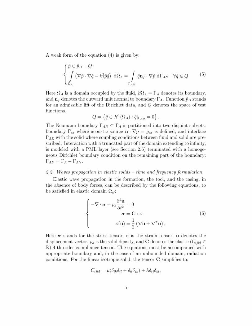
A weak form of the equation (4) is given by:p ∈ pD +Q :∫ΩA

(∇p · ∇q − k2

f pq)

dΩA =

∫ΓAN

qnf · ∇p dΓAN ∀q ∈ Q (5)

Here ΩA is a domain occupied by the fluid, ∂ΩA = ΓA denotes its boundary,and nf denotes the outward unit normal to boundary ΓA. Function pD standsfor an admissible lift of the Dirichlet data, and Q denotes the space of testfunctions,

Q =q ∈ H1(ΩA) : q|ΓAD

= 0.

The Neumann boundary ΓAN ⊂ ΓA is partitioned into two disjoint subsets:boundary Γex where acoustic source n · ∇p = gex is defined, and interfaceΓAE with the solid where coupling conditions between fluid and solid are pre-scribed. Interaction with a truncated part of the domain extending to infinity,is modeled with a PML layer (see Section 2.6) terminated with a homoge-neous Dirichlet boundary condition on the remaining part of the boundary:ΓAD = ΓA − ΓAN .

2.2. Waves propagation in elastic solids – time and frequency formulation

Elastic wave propagation in the formation, the tool, and the casing, inthe absence of body forces, can be described by the following equations, tobe satisfied in elastic domain ΩE:

−∇ · σ + ρs∂2u

∂t2= 0

σ = C : ε

ε(u) =1

2

(∇u +∇Tu

),

(6)

Here σ stands for the stress tensor, ε is the strain tensor, u denotes thedisplacement vector, ρs is the solid density, and C denotes the elastic (Cijkl ∈R) 4-th order compliance tensor. The equations must be accompanied withappropriate boundary and, in the case of an unbounded domain, radiationconditions. For the linear isotropic solid, the tensor C simplifies to:

Cijkl = µ(δikδjl + δilδjk) + λδijδkl,

5

where λ and µ denote (real) Lame coefficients. The Lame coefficients canbe defined through characteristic wave speeds in the solid, namely: P-wavespeed vp, and S-wave speed vs,

µ = ρsv2s λ = ρs(v

2p − 2v2

s). (7)

Applying Fourier transform in time, we obtain the corresponding equa-tions in the frequency domain:

−∇ · σ − ρsω2u = 0

σ = C : ε

ε(u) =1

2

(∇u +∇T u

),

(8)

where σ, ε, and u denote the Fourier transforms of the appropriate quanti-ties.

The equations are equipped with two kinds of boundary conditions: ho-mogeneous displacement (Dirichlet) BC imposed on part of the boundaryΓED ⊂ ΓE, ΓE = ∂ΩE, and (Neumann) tractions BC ns · σ = t prescribedon the remaining part of the boundary ΓEN = ΓE −ΓED. Here ns stands forthe outward unit normal to boundary ΓE.

A weak form of the equation (8) is given by:u ∈ uD + W :∫ΩE

(εw : C : εu − ρsω2u · w

)dΩE =

∫ΓEN

t · w dΓEN ∀w ∈W (9)

where uD is an admissible lift of the Dirichlet data, and W is the space oftest functions defined by:

W =w ∈ H1(ΩE) : w|ΓED

= 0.

The Neumann boundary ΓEN is then divided into two disjoint parts: ΓEAwhere coupling conditions between solid and fluid are prescribed, and theremaining part on which zero traction is prescribed. Similarly to the acous-tic case, the interaction with an unbounded part extending to infinity istruncated with a PML layer (see Section 2.6) terminated with homogeneousDirichlet boundary conditions.

6

2.3. Coupling conditions between fluid and solid

Coupling conditions at the interface between fluid and solid assure thecompatibility of displacements, i.e. the equality of the normal component ofvelocities:

nf · v = nf · (iωu),

and tractions:t = ns · σ = −nsp.

Using equation (32), the first condition can be expressed as:

nf · ∇p = ρfω2nf · u.

Thus, finally, the weak form for the coupled acoustic-elastic problem isgiven by:

(u, p) ∈ (uD, pD) + W ×Q :

bAA(p, q) + bAE(u, q) = lA(q) ∀q ∈ Q,bEA(p, w) + bEE(u, w) = 0 ∀w ∈W,

where:

bAA(p, q) =

∫ΩA

(∇p · ∇q − k2

f pq)

dΩA

bAE(u, q) = −∫

ΓAE

ρfω2qnf · u dΓAE

bEA(p, w) =

∫ΓEA

pns · w dΓEA

bEE(u, w) =

∫ΩE

(εw : C : εu − ρsω2u · w

)dΩE

lA(q) =

∫Γex

qgex dΓex

2.4. Modeling anelastic attenuation

It is observed fact that energy of the elastic waves in the formation ex-hibits some damping due to internal friction, presence of fluids and a non-homogeneous structure of the formation (grains, crystal imperfections, frac-tures, etc) [10]. The attenuation is frequency dependent and has stronger

7

effects for higher frequencies causing a decrease of the wave amplitude andchange of wave velocity. Several methods have been developed to deal withthe attenuation [23]. One of the classical approaches describing this phe-nomenon is based on the theory of viscoelasticity which complements theclassical elastic theory strain with velocity dependent terms. Consequently,the stress does not depend solely on the strain but also takes into accountthe strain history. Another approach used to model the attenuation phe-nomenon is ”an analysis based on the constraints imposed by causality onwave propagation”. We follow the second method and use constant-Q model[24].

We define the complex wavenumbers, complex wave velocities and com-plex compliance tensor to modify the classical elastic equations. Lame coef-ficients are defined by characteristic wave velocities in the solid (equations7). Additional parameters describing attenuation in the model are so calledquality factors Qp and Qs which express the damping rate in one wave cy-cle. In the presented model, one assumes that these factors are frequencyindependent. The method defines the complex phase velocity:

c(ω) = c0

(1 +

1

πQlnω

ω0

)(1 +

i

2Q

), (10)

where c0 is a reference velocity at angular frequency ω0. The authors suggestto use a reference frequency 1Hz [24], that corresponds to angular frequencyω0 = 2π. The equation above is often replaced with a simpler version, ne-glecting the term with factor 1/Q2. The same approach can be used to modelattenuation in a fluid which for the presented problem can represent wateror oil base mud, hydrocarbon or brine present in the formation cracks. Theincrease of seismic velocities with frequency agrees with experiments over therange of frequencies from 100Hz–100kHz [11].

Having given pairs (v0p, Qp) and (v0

s , Qs) and setting ω0 = 2π, one cancalculate complex phase velocities:

vp = v0p

(1 +

1

πQp

ln f

)(1 +

i

2Qp

),

vs = v0s

(1 +

1

πQs

ln f

)(1 +

i

2Qs

),

where v0p and v0

s are low frequency limit reference velocities, and f denotesthe frequency.

8

Thus, accounting for the attenuation in the wave propagation problem,one simply has to replace characteristic wave velocities with the complexvelocities, resulting in the corresponding complex and frequency dependentacoustic wavenumber kf , and solid compliance tensor C.

2.5. Modeling of multipole acoustic sources

Almost all logging tools are based on a combination of monopole, dipoleor quadrupole acoustic sources. A proper numerical model for such sourcesis needed.

A monopole source can be modeled with an acoustic point source whichexhibits spherical symmetry pattern of the radiation. Multipole sources oforder n can be constructed from the collection of 2n monopole point sourcesplaced periodically in the same plane, along a circle of radius r0, alternat-ing in sign [25]. Furthermore, such a model of the multipole source can be

+

Monopole

n = 0

+−

Dipole

n = 1

+

−

+

−

Quadrupole

n = 2

Figure 1: Models for multipole acoustic sources

approximated with a Fourier expansion in the azimuthal direction θ. Themonopole source is 0 order, dipole source is of the 1st order and consists oftwo point sources of opposite sign, an the quadrupole source consists of fourmonopole sources, located at angles kπ/2. The leading term in the radia-tion pattern for the n-order multipole source exhibits cos(nθ) dependence inazimuthal angle θ (see Fig. 1). Therefore, one can approximate a multipolesource of order n by:

g(n)ex = p0 cos(nθ) =

p0

2einθ︸︷︷︸g+n

+p0

2e−inθ︸︷︷︸g−n

n = 0, 1, 2, . . . (11)

Use of complex exponentials instead of the cosine function enables a furthersimplification of the variational formulation of the problem in cylindrical co-ordinates, and makes possible to decrease the dimension of the calculated

9

problem. Due to the linearity of the problem, solution (pn, un) of n-th az-imuthal order can be computed as a superposition of solutions (p+

n , u+n ) and

(p−n , u−n ) calculated independently for exciting sources g+

n and g−n respectively.Assuming an excitation of the form given by g+

n we arrive at the followingdefinitions of trial and test functions:

p+n = pn(r, z)einθ un = un(r, z)einθ

q+n = qn(r, z)e−inθ wn = wn(r, z)e−inθ (12)

where pn, qn, un and wn are solely functions of r and z coordinates.

Monopole source (n = 0).. The source excites only one mode. Consequently,one can solve the problem with excitation source equal g+

n , and then multiplythe solution by 2. The source pattern is axially symmetric, the solution doesnot depend upon the azimuthal direction θ and, therefore, can be directlysolved for in 2D (r, z) domain. Furthermore, the test and trial functions are ofthe same form which implies for the presented problems a (complex-valued)symmetric stiffness matrix.

Multipole source (n > 0).. The source excites two modes. In this case, itis still enough to calculate only solution (pn, un) for excitation g+

n , how-ever, the bilinear form is now not symmetric and contains all terms. Dueto symmetries and antisymmetries in bilinear forms b+

n ((p+, u+), (q+, w+)),and b−n ((p−, u−), (q−, w−)), one can observe that:

b−n((p−, u−r , u

−θ , u

−z ), (q−, w−r , w

−θ , w

−z ))

=

b+n

((p+, u+

r ,−u+θ , u

+z ), (q+, w+

r ,−w+θ , w

+z ))

and furthermore, the load vectors for both cases are the same, because:

g+n q

+ = g−n q− =

p0

2qn(r, z).

Thus, the solution for the problem with excitation g−n can be directly calcu-lated from the solution of the problem with excitation g+

n , which halfs thecomputational time. Components p, ur, uθ and uz for constant values of nare solely functions of r and z coordinates enabling thus the solution only in2D trace (r, z) domain.

10

The final solution (pn, un) is calculated in terms of the solution for oneexcitation mode only, as follows:

pn =1

2

(p+einθ + p−e−inθ

)= p+ cos(nθ) (13)

un =1

2

u+r e

inθ

u+θ e

inθ

u+z e

inθ

+

u−r e−inθu−θ e−inθ

u−z e−inθ

=

u+r cos(nθ)

u+θ i sin(nθ)u+z cos(nθ)

(14)

Transforming the solution into time domain.. Having calculated solutions forsufficiently many frequencies, the inverse Fourier transform 1 is performeddelivering the solution in time domain:

p(x, t) =1

2π

∫ ∞−∞

p(x, ω)eiωt dω ≈ ∆ω

2π

c∑n=−c

p(x, ωn)eiωnt (15)

u(x, t) =1

2π

∫ ∞−∞

u(x, ω)eiωt dω ≈ ∆ω

2π

c∑n=−c

u(x, ωn)eiωnt, (16)

where ∆ω is a chosen frequency step, c is a number of discrete frequenciesused, and ωi = n∆ω is a discrete angular frequency. The frequency spacing∆ω should be chosen in such a way that ∆ω < π

T, where 2T is an anticipated

simulation time.The number of needed frequencies c depends on the spectrum of exci-

tation and the response. In particular, if the excitation source has a com-pact/narrow spectrum and that spectrum decays quickly with increasing fre-quency then one can neglect higher frequencies for which the spectrum isnegligibly small.

2.6. Perfectly Matched Layer (PML)

A general problem of wave propagation in a borehole–formation systemis posed in an unbounded domain. An effective numerical simulation of thisproblem using FEM needs a truncated domain, and special techniques areneeded for truncating boundary conditions to avoid reflections of outwardpropagating waves. For this purpose, the PML method was used.

For the problem defined in frequency domain, and cylindrical coordinates(r, θ, z) the PML absorbing layer is constructed by a complex stretching of

1We use the inverse FFT in actual computations.

11

the axial (z) and radial (r) coordinates. Given a wavenumber k, we use thefollowing transformation:

xj := Xj(xj, k)∂

∂xj:=

1

X ′j

∂

∂xjwhere X ′j =

∂Xj

∂xj. (17)

The transformation of coordinates xj results in an analytic continuation ofthe solution into a complex plane characterized with an exponential decay ofthe outgoing waves, and an exponential blow-up of the incoming waves in thestretched direction (r or z) within the PML absorbing region. Consequently,imposing a homogeneous Dirichlet boundary at the end of the PML regiondoes not affect the (“stretched”) outgoing wave but it eliminates the incomingone. It is of a utmost practical importance to construct the stretching in sucha way that the attenuated outgoing wave reaches a machine zero on the PMLouter boundary.

The general form of the stretching transformation in direction Xj can bewritten as follows:

Xj(xj, k) = gj(xj, k)(1− i) + xj (18)

X ′j(xj, k) = g′j(xj, k)(1− i) + 1 (19)

X ′′j (xj, k) = g′′j (xj, k)(1− i) (20)

where i is an imaginary unit and a function gj(xj, k) is defined by:

gj(xj, k) =2p

ka(ξ)m

ξ′

|ξ′| where [0, 1] 3 ξ(xj) =

xLj −xjδj

xj < xLjxj−xRjδj

xj > xRj

0 otherwise.

(21)

The simultaneous stretching of both real and imaginary parts produces aneffect that not only the plain waves but also evanescent waves are dampedwithin the PML region. Computational domain in xj-direction is containedin [xLj − δj, xRj + δj], x

Lj < xRj , where δj is the PML width in xj-direction.

Function a maps [0, 1] onto itself. Parameter p controls the strength of thewave attenuation. For instance, it can be estimated as

p >ln(d ln 10)

ln 2

if we want to decrease amplitude of the incident wave by factor 10d. Forp = 5, the wave amplitude attenuation on the outer boundary of the PML is

12

Name a

(ver-1) ξ

(ver-2) ξ − sin 2πξ2π

(Bramble-Pasciak)[26] ξ3[10− ξ(15− 6ξ)]

Table 1: Proposed choices of auxiliary stretching functions a.

of order 10−14, and for p = 6 the amplitude decrease is of order 10−28, which– assuming wave amplitudes of order 1 into the simulated domain – givesvalues below the machine zero on a standard computer.

The last step in definition of stretching function g is the definition ofauxiliary function a : [0, 1] → [0, 1] such that a(0) = 0 and a(1) = 1. Theterm am controls the way in which the attenuation of the wave is increasedas we go deeper into the absorbing layer. Some choices of the function a arepresented in Table (1).

2.7. Formulation in cylindrical coordinates

The cylindrical coordinates, due to the axial symmetry of the geometryof the problem, as well as due to convenient approach for the representationof multipole nonsymmetric sources (presented in the previous sections), area natural choice for the presented problem.

Formulation for acoustics.. First, one has to define gradients of the functionsp and q under PML stretching and using function definitions (12):

∇p =

[∂p

∂r,1

r

∂p

∂θ,∂p

∂z

]PML, (12)−−−−−−→

[1

R′∂pn∂r

,+inpnR

,1

Z ′∂pn∂z

]einθ

∇q =

[∂q

∂r,1

r

∂q

∂θ,∂q

∂z

]PML, (12)−−−−−−→

[1

R′∂qn∂r

,−inqnR

,1

Z ′∂qn∂z

]e−inθ

Now, taking into account that the jacobian dΩA = r dr dθ dz is transformed,due to the PML stretching, into dΩA = RR′Z ′ dr dθ dz, one arrives at thefinal weak form for acoustic equation:∫

ΩA

(RZ ′

R′

)∂pn∂r

∂qn∂r

+

(RR′

Z ′

)∂pn∂z

∂qn∂z

+

(n2R

′Z ′

R− k2

fRR′Z ′)pnqn dΩA

− ρfω2

∫ΓAE

qnnf · uRR′Z ′ dΓAE =

∫Γex

qnp0

2RR′Z ′ dΓex ∀qn ∈ Q. (22)

13

The corresponding energy space is defined as a weighted H1 space:

Q =

q :

∣∣∣∣RZ ′R′

∣∣∣∣ 12 ∂q∂r ,∣∣∣∣RR′Z ′

∣∣∣∣ 12 ∂q∂z , n∣∣∣∣R′Z ′R

∣∣∣∣ 12 q, |RR′Z ′| 12 q ∈ L2(ΩA), q|ΓAD= 0

Formulation for elasticity.. In here, one has to first define strain tensor com-ponents expressed in cylindrical coordinates:

εrr =∂ur∂r

εrz =1

2

(∂ur∂z

+∂uz∂r

)εzz =

∂uz∂z

εrθ =1

2

[∂uθ∂r− 1

r

(uθ −

∂ur∂θ

)]εθθ =

1

r

(∂uθ∂θ

+ ur

)εθz =

1

2

(∂uθ∂z

+1

r

∂uz∂θ

)perform an analogous PML stretching, and introduce function definitions (12):

εrr(u) = α1

R′∂ur∂r

εrr(w) = β1

R′∂wr∂r

εzz(u) = α1

Z ′∂uz∂z

εzz(w) = β1

Z ′∂wz∂z

εθθ(u) = α1

R(ur + inuθ) εθθ(w) = β

1

R(wr − inwθ)

εrz(u) = α1

2

(1

Z ′∂ur∂z

+1

R′∂uz∂r

)εrz(w) = β

1

2

(1

Z ′∂wr∂z

+1

R′∂wz∂r

)εrθ(u) = α

1

2

(1

R′∂uθ∂r− uθ − inur

R

)εrθ(w) = β

1

2

(1

R′∂wθ∂r− wθ + inwr

R

)εθz(u) = α

1

2

(1

Z ′∂uθ∂z

+inuzR

)εθz(w) = β

1

2

(1

Z ′∂wθ∂z− inwz

R

)where we have dropped subscript n for displacement components, α = einθ

and β = e−inθ = 1/α. Thus, for the most general considered case we have:

εw : C : εu = (2µ+ λ) [εrr(u)εrr(w) + εθθ(u)εθθ(w) + εzz(u)εzz(w)] (23)

+ λ [εrr(u)εθθ(w) + εθθ(u)εrr(w) + εrr(u)εzz(w)]

+ λ [εzz(u)εrr(w) + εθθ(u)εzz(w) + εzz(u)εθθ(w)]

+ 4µ [εrθ(u)εrθ(w) + εrz(u)εrz(w) + εθz(u)εθz(w)]

14

and the final equation for elasticity is obtained from the second equation (9)replacing εw : C : εu term according to definition (23), and taking intoaccount stretching jacobian factor RR′Z ′ in each integral.

In the case of a monopole source (n = 0, fully axisymmetric problem), thebilinear form decouples into two independent bilinear forms, where the firstdepends only on r and z components and the second on θ component only.Similar decomposition follows for the load vector. Assuming that uθ = 0,solution reduces to determining the ur and uz components only, and the finalbilinear and linear forms simplify to r and z dependent counterparts.

The energy space for the PML formulation is defined analogously to theacoustic case as a weighted H1 space.

2.8. Alternative choice of unknowns

Looking at the integrals contributing to the energy norm (22,23), wearrive at the problem of securing additional conditions assuring finiteness ofthe energy at the axis of symmetry (r = 0).

Let us consider first the monopole case. The acoustic bilinear form con-tains no singular terms but the elastic bilinear form for elasticity includes asingular term εθθ = ur/r. Two possible scenarios can occur. If the elastic ma-terial is placed off of the axis of symmetry (open borehole or logging–while–drilling (LWD) tools), there is no singularity in the elastic energy functional.However simulation of a wireline (solid) tool leads to the presence of thesingular term in the elastic energy.

Two solutions are presented to overcome this problem. In the first (wecall this approach ”formulation A” hereafter), no conditions are prescribedon the axis of symmetry in the elastic domain. Consequently, for all elementsadjacent to the axis of symmetry, no additional boundary integrals are com-puted. As the volume integrals are computed using standard (non-adaptive)Gauss quadrature, integration of the singular term results effectively in animplicit penalty term which forces the radial displacement component ur tovanish on the axis of symmetry.

A similar situation occurs for the multipole sources (n > 0). In herehowever, there are more singular terms in the energy norms, in acousticswe have the term p2/r2, and in elasticity we have term εθz ∼ uz/r, as wellas terms εθθ and εrθ which are proportional to linear combinations of (ur +iuθ)/r. Therefore, for each possible geometry of the problem, the presentedphenomenon exists.

15

Another approach, which we call the ”formulation B” deals with theproblem through a proper choice of alternative independent variables. Formonopole sources, we consider new variables u′r, u

′z, p

′ defined as:

ur = ru′r uz = u′z p = p′.

Therefore, now the term εθθ is proportional to u′r, and it is automaticallyequal zero for r = 0 which in turn makes the elastic energy finite. Thestretched strain tensor for monopole source has the following components:

εrr(u′) = α

1

R′

(u′r + r

∂u′r∂r

)εrr(w

′) = β1

R′

(w′r + r

∂w′r∂r

)εzz(u

′) = α1

Z ′∂u′z∂z

εzz(w′) = β

1

Z ′∂w′z∂z

εθθ(u′) = α

ru′rR

εθθ(w′) = β

rw′rR

εrz(u′) = α

1

2

(r

Z ′∂u′r∂z

+1

R′∂u′z∂r

)εrz(w

′) = β1

2

(r

Z ′∂w′r∂z

+1

R′∂w′z∂r

)”Formulation B” for a multipole source is obtained through the following

choice of the independent variables:

ur = u′r uz = ru′z uθ = u′θ p = p′.

Therefore acoustic energy and the εθz are finite at the axis of symmetry.We are still left with singular terms εθθ and εrθ. The ansatz to enforce anautomatic vanishing of the quantity (ur+iuθ)/r at r = 0 requires consideringvector-valued shape functions for elasticity and it is much more difficult toimplement. The stretched strain tensor for monopole source has the followingcomponents:

εrr(u′) = α

1

R′∂u′r∂r

εrr(w′) = β

1

R′∂w′r∂r

εzz(u′) = α

r

Z ′∂u′z∂z

εzz(w′) = β

r

Z ′∂w′z∂z

εθθ(u′) = α

1

R(u′r + inu′θ) εθθ(w

′) = β1

R(w′r − inw′θ)

εrz(u′) =

α

2

(1

Z ′∂u′r∂z

+r

R′∂u′z∂r

+u′zR′

)εrz(w

′) =β

2

(1

Z ′∂w′r∂z

+r

R′∂w′z∂r

+w′zR′

)

16

εrθ(u′) = α

1

2

[1

R′∂u′θ∂r− u′θ − inu′r

R

]εrθ(w

′) = β1

2

[1

R′∂w′θ∂r− w′θ + inw′r

R

]εθz(u

′) = α1

2

(1

Z ′∂u′θ∂z

+inru′zR

)εθz(w

′) = β1

2

(1

Z ′∂w′θ∂z− inrw′z

R

)3. hp Technology

3.1. A new hp-FE code for multiphysics problems

The presented work has been implemented within a new version of our 2Dhp code for coupled, multiphysics problems [4]. The principal characteristicson the new code include:

• support of discretizations using a simultaneous use of all elements form-ing the exact sequence: H1-, H(curl)-, H(div)-, and L2-conformingelements 2,

• support of (weakly) coupled problems,

• energy driven automatic hp-adaptivity [2, 3]

In particular, the discussed project led to a non-trivial modification of theautomatic hp-adaptivity algorithm for a coupled problem (different systemsof equations in different parts of the domain) discussed below.

3.2. Modification of hp algorithm for coupled multiphysics problems throughautomatic norm scaling

The hp-algorithm two-grid paradigm is based on calculating local energynorms on element edges and in element interiors. In the presented case wedeal with two different media, solid and fluid, and thus different physical phe-nomena and different quantities for which we solve the system of equations –elastic displacements and acoustic pressure. The energy norms correspond-ing to the two problems have dramatically different values, even if a standardnon-dimensionalization is used. In the examples to follow, the energy normin the acoustical domain was typically larger than the one in the elastic do-main, by several orders of magnitude. This implies that the resolution of theelastic part of the domain becomes of a secondary importance. Large differ-ences in energy lead also to possible conditioning problems, even if a direct

2Only H1-conforming elements are used in this project.

17

solver is used. This can be observed e.g. by monitoring pivots reported bythe solver.

Therefore, a key-point to a successful application of the automatic hpadaptivity to the coupled problem is to rescale the governing equations tobalance quantitatively the acoustic and elastic energy norms. Once the equa-tions are rescaled in such a way that energy norms for a current hp step areequal then the comparison of relative errors in both domains will be mean-ingful and thus fully justified.

Let u = suu and p = spp. This implies the following scaling for linearand bilinear forms:

spsubAA(p, q) + bAE(u, q) =

1

sulA(q) ∀q ∈ Q,

bEA(p, w) +suspbEE(u, w) = 0 ∀w ∈W,

and the corresponding scaling for the norms:

‖|p‖|A = sp‖|p‖|A ‖|u‖|E = su‖|u‖|E.

Now, if we set sp = ‖|p‖|A and su = ‖|u‖|E, then the energy norms of thescaled solutions ‖|p‖|A and ‖|u‖|E be of order 1. Consequently, that enablesto compare relative errors of both solutions.

The modified automatic hp algorithm has now the form:

1. set sp = su = 1,

2. solve the problem for (u, p)

3. save new values s′p = ‖|p‖|A and s′u = ‖|u‖|E4. FOR each hp step DO

(a) set sp ← s′p, su ← s′u,(b) perform classical hp-step, calc new solution (u, p),(c) save new values s′p = sp‖|p‖|A and s′u = su‖|u‖|E

4. Verification of the code

Before we continue with several practical examples, we would like topresent necessary steps we have taken to verify the code and justify thechoice of several parameters like the frequency range or PML parameters.The verification process has been carried out in several steps, starting withdecoupled acoustic and elastic problems for which analytical solutions exist,

18

and continuing then with the coupled problem and comparisons with othersoftware.

The ultimate results are produced in the time-domain through the appli-cation of the inverse Fourier transform integrated numerically, and the firsttechnical decisions concerned the necessary frequency range for the simula-tions.

4.1. Acoustic source model

The most frequently used model for a sonic source in borehole simulationsis the Ricker wavelet, see Fig. 2, due to its fast decay in both time andfrequency domains [24]:

p(t) =2√π

[1− 2

(t− t0T

)2]e−( t−t0

T )2

(24)

p(ω) = 4Te−iωt0Ω2e−Ω2

Ω =ωT

2= πfT. (25)

In the above, t0 is a time at which maximum of the pulse occurs and T = 1πfc

is a characteristic period of the pulse defined by so called central frequency fc.Given a central frequency fc, the frequency spectrum of the Ricker wavelet

−1 0 1 2 3 4 5 6−0.6

−0.4

−0.2

0

0.2

0.4

0.6

0.8

1

1.2Ricker wavelet

Time

Am

plitu

de

0 2 4 6 8 100

0.05

0.1

0.15

0.2

0.25Ricker wavelet

Frequency

Am

plitu

de

Figure 2: Ricker wavelet: fc = 2, t0 = 2.

is essentially contained between 0 and 3fc which is sufficiently accurate inapplication to the presented cases. Using this rule, one can easily estimatethe required frequency range in typical well-logging applications [12]:

• for a monopole source, we will use central frequency fc = 8 kHz, thatgives range (0, 25) kHz; in this case the frequency step equal 50 Hz willbe used;

19

• for a dipole and a quadrupole source we will use fc = 2 kHz or fc =3 kHz, which gives ranges (0, 6) kHz and (0, 9) kHz respectively; forthese cases the 25 Hz frequency step will be used.

4.2. Pure acoustic case

For the purpose of verifying the acoustic part of the hp multiphysicscode, two different cases were considered: with a point source (Fig. 3(a))and a ring source (Fig. 3(b)). The fluid density ρf = 1000 kg/m3 and soundspeed cf = 1500 m/s were used in both cases. In the first case (Fig. 3(a)), the

PML

PML

PMLr

z

0.5

1.0

d

FLUID

0.5

0.05

d

d

Q

(a) Point source

PML

PML

PML

FLUID

r

z

0.5

1.0

d

0.5

d

d

0.05

0.05

Q

(b) Ring source

Figure 3: Geometries for the pure acoustic problems.

calculated solution is compared to the analytical solution for the Helmholtz

20

equation for point monopole and dipole sources. The fluid pressure for amonopole point source in cylindrical coordinates is given by:

pM(r, z) =1

4πRe−ikfR R =

√r2 + z2.

The field is spherically symmetric.The dipole acoustic source is realized by placing two monopole sources

of opposite sign at [d, 0, 0] and [d, π, 0] (2d is the distance between the twomonopoles that constitute the acoustic dipole) which results in the pressurepattern that exhibits cosφ azimuthal dependence and it is axially symmetricwith respect to z-axis. Thus it conforms to the assumptions for multipolesources presented in Section 2.5. The pressure field is given by:

pD(r, z) = − d

2πR

(1

R+ ikf

)e−ikfR

r cos θ

R,

where θ is the azimuthal angle. In the presented cases, a value d = 0.01 mwas used.

For both monopole and dipole source, the problem is solved in [0, 0.5]×[−0.5, 1] m domain with the circular hole of radius 5 cm surrounding the pointsource cut (see Fig. 3(a)). The source is introduced through the Neumannboundary condition prescribed on the edge of the circular hole.

In the second case (Fig. 3(b)), the ring source is modeled as a super-position of monopole point sources placed around a circle of radius 5 cm,perpendicular to the z-axis. This case is more realistic for the borehole soniclogging and reflects the construction of real monopole sources used in wire-line logging tools. The analytical equation describing acoustic field pressuregenerated by such a source (of 0 thickness) is given by [27]:

p(r, z) =a

4π

2π∫0

e−ikfR

Rdθ R2 = r2 + a2 − 2ar cos θ + z2,

where a is the ring radius and the integration is performed in the azimuthaldirection. Here, a numerical integration is needed to calculate the solutionand solution derivatives at a point. We used the Romberg’s method for thatpurpose. The source is introduced through the Neumann boundary conditionprescribed on the edges of a square hole surrounding the ring source.

21

(a) Fine mesh (b) Re(p)

(c) log |pf − pex| (d) Re(p) (red) and |p| (blue) alongthe profile (zoomed in PML zone, PMLmarked in blue)

Figure 4: Acoustics. Dipole point source. Formulation A. f = 25 kHz

22

As an example, in Figure 4 we present the results of the simulation foracoustic dipole at frequency 25 kHz. The final hp-refined optimal mesh ispresented in subfigure (a). Colors are used to indicate the orders of partic-ular edges and element interiors, according to the enclosed scale. One canobserve that the mesh refinements conform the solution distribution (pre-sented in subfigure (b)): e.g. solution along z-axis for dipole is very small,thus the corresponding elements are relatively large and use lower orders ofapproximation). Accurate resolution of the large gradients of the solutionwithin the PML results in appropriate mesh refinements close to the PMLinterface.

In subfigure (c), logarithm of the modulus of the difference between cal-culated and analytical solution is plotted. This provides an insight on theerror distribution over the mesh. For solution magnitude of order 1, the ob-served error is of order 10−7 and less. Higher values of the error are encoun-tered within the PML layer; the PML stretched solution exhibits a strongboundary layer whose resolution is more demanding and results in extensiverefinements. Nevertheless, the larger error in the PML region does not seemto affect the error within the domain of interest.

Behavior of the solution within the PML layer is presented in subfigure(d). The solution is plotted along profile Q (see Figure 3 for the definitionof the profile). We show here the real part and the modulus of the pressure.The beginning of the PML is indicated by the vertical line; PML continuesthen to the right. One can observe that the solution is properly damped andattains the machine zero value at 2/3 of the PML depth.

The remaining examples are presented in Appendix Appendix A: withthe monopole point source at frequency 50 Hz (Figure A.30) and 25 kHz (Fig-ure A.31), with the monopole ring source at frequency 50 Hz (Figure A.32)and 25 kHz (Figure A.33), with the dipole source at frequency 50 Hz (Fig-ure A.34 for formulation A and Figure A.35 for formulation B) and 25 kHz(Figure A.36 for formulation B).

The PML technique works properly in both low and high frequencyregime. The automatically generated mesh refinements for low and highfrequency cases, reflect well the fact that the hp algorithm aims at minimiz-ing the error in the energy norm. For low frequencies, the solution within thedomain of interest changes very slowly (wavelength for the simulated fluidat 50 Hz is 30 m) and is very smooth – large elements with high polynomialorder are used. On the other side, the solution within the PML has highgradients and thus high energy error, which in turn produces most of the

23

refinements in that layer and results in generation of much smaller elementsof lower order in the hp-refined mesh.

For high frequencies, the energy distribution is more balanced which isreflected in a more uniform distribution of the refinements throughout themesh. The size of mesh elements is also related to the smallest wavelength(for the simulated fluid at 25 kHz, λ = 6 cm).

All presented examples show that the self-adaptive hp code is able to ac-curately resolve the acoustic wave propagation problem for multipole sourcesat the range of frequencies [50 − 25000] Hz. Convergence curves (for pointmonopole in Figure 5, for ring monopole in Figure 6, for dipole in Figure 7for formulation A, and in Figure 8 for formulation B, respectively) obtainedfor all test problems indicate at least an algebraic convergence. In each plotwe present three curves corresponding to:

• relative energy error of the coarse solution with respect to the fine mesh(red curve),

• relative energy error of the coarse solution with respect to the analyticalsolution (black curve), and

• relative error of the fine solution with respect to the analytical solution(blue curve).

We remind the reader that refinements of the coarse grid are driven bythe fine grid solution. The kinks present in the convergence curves resultfrom an introduction of new scales in the fine grid solution that successfullyenter the picture as the mesh is refined (see [2], Section 15.3 for a relateddiscussion).

4.3. Pure elastic case

For the verification of the elastic part of the hp multiphysics code, thecase with a source placed at the origin of the coordinate system surroundedby a circular hole was considered (Fig. 3(a)). In all tests, a homogenousfast formation was assumed, described by the following parameters: ρs =2200 kg/m3, vp = 3048 m/s, vs = 1793 m/s, and both quality factors equal∞ (no anelastic attenuation).

The analytical solutions for displacements excited by a monopole or dipoleimpulsive source can be developed from the Stokes-Love solution for the

24

1 0 3 1 0 41 E - 4

1 E - 3

0 . 0 1

0 . 1

1

1 0

Relat

ive en

ergy e

rror, %

# D O F S

E r r ( U c , U e x ) E r r ( U c , U f ) E r r ( U f , U e x )

C o n v e r g e n c e

(a) f = 50 Hz

1 0 4 1 0 5

1 E - 3

0 . 0 1

0 . 1

1

1 0

Relat

ive en

ergy e

rror, %

# D O F S



(b) f = 25 kHz

Figure 5: Convergence for acoustics. Monopole point source. Formulation A.

1 0 3 1 0 4 1 0 5

1 E - 3

0 . 0 1

0 . 1

1

1 0

1 0 0

Relat

ive en

ergy e

rror, %

# D O F S



(a) f = 50 Hz

1 0 4 1 0 5

1 E - 3

0 . 0 1

0 . 1

1

1 0

Re

lative

energ

y erro

r, %

# D O F S



(b) f = 25 kHz

Figure 6: Convergence for acoustics. Ring source. Formulation A.

1 0 3 1 0 4

0 . 0 1

0 . 1

1

1 0

Relat

ive en

ergy e

rror, %

# D O F S



(a) f = 50 Hz

1 0 4 1 0 51 E - 3

0 . 0 1

0 . 1

1

1 0

Relat

ive en

ergy e

rror, %

# D O F S



(b) f = 25 kHz

Figure 7: Convergence for acoustics. Dipole point source. Formulation A.

25

1 0 3 1 0 4

0 . 0 1

0 . 1

1

1 0

Re

lative

energ

y erro

r, %

# D O F S



(a) f = 50 Hz

1 0 4 1 0 5

1 E - 3

0 . 0 1

0 . 1

1

1 0

Relat

ive en

ergy e

rror, %

# D O F S



(b) f = 25 kHz

Figure 8: Convergence for acoustics. Dipole point source. Formulation B.

Navier equations given in frequency domain [28]:

v2p∇∇ · u− v2

s∇×∇× u + ω2u = − f

ρs,

where f is the impulsive source of a force magnitude F0, concentrated at thepoint r0, acting in direction a and expressed by:

f = F0(ω)δ(r− r0)a,

where a is a unit vector, and δ denotes the Dirac distribution. We taker0 = 0. Solution of the problem in cylindrical coordinates is given by:

ui = F0Gijaj,

where Gij is the Green’s dyadic which gives the i-th component of the dis-placement for force acting along the j-th direction. The Green’s diadic incylindrical coordinates (r, θ, z) is given by:

Gij(x,y;ω) =1

4πρω2

k2βS +

∂2Q

∂r20

∂2Q

∂r∂z

0 k2βS +

1

r

∂Q

∂r0

∂2Q

∂r∂z0 k2

βS +∂2Q

∂z2,

26

where:

P (R) =e−ikpR

Rkp =

ω

vp,

S(R) =e−iksR

Rks =

ω

vs,

Q(R) = S(R)− P (R) R = |r− r0| .

For r0 = 0, one can observe that R as well as P (R), S(R) and Q(R) do notdepend upon the azimuthal coordinate θ.

Monopole. We consider an impulsive source, placed at the origin and act-ing along the z-axis. Then the cylindrical components of vector a = z are[0, 0, 1]T . Thus the displacement can be calculated from the formula:

uM =F0

4πρω2

∂2Q

∂r∂z

0

∂2Q

∂z2+ k2

βS

=Q

4πρω2

(∂2Q

∂R2− 1

R

∂Q

∂R

)γrγz

0

∂2Q

∂R2γ2z +

1

R

∂Q

∂Rγ2r + k2

βS,

where γi =

∂R

∂xi=

xiR

. An important observation is that the azimuthal

displacement component is equal 0, i.e. the solution is axially symmetricwith respect to the z-axis. This implies, that we can model this problemusing the source model of 0th order (i.e. the monopole version of the code).

Dipole. We consider an impulsive source, placed at the origin and actingalong the r-axis. The cylindrical components of vector a = r are [cos θ,− sin θ, 0]T .

27

Thus the displacement can be calculated from the formula:

uD =F0

4πρω2

(k2βS +

∂2Q

∂r2

)cos θ

−(k2βS +

1

r

∂Q

∂r

)sin θ

∂2Q

∂r∂zcos θ

=F0

4πρω2

cos θ

(k2βS +

∂2Q

∂R2γ2r +

1

R

∂Q

∂Rγ2z

)− sin θ

(k2βS +

1

R

∂Q

∂R

)cos θ

(∂2Q

∂R2− 1

R

∂Q

∂R

)γrγz.

In this case, the azimuthal displacement is non-zero. The important obser-vation here is that both ur and uz components of the displacement exhibitdependence of θ which is exactly given by cos θ and the uθ component dependsupon the azimuthal coordinate through − sin θ relationship. Comparing thiswith equation (14) one can see, that the pattern of the solution uD corre-sponds to the solution un up to the multiplication of the second componentof uD by factor −i.

This means that one can use a dipole version of the code (with n = 1)for the solution of elastic wave propagation problem with the exact solutiongiven in trace domain (i.e. (r, z)-plane) by:

uD(r, z) =F0

4πρω2

(k2βS +

∂2Q

∂R2γ2r +

1

R

∂Q

∂Rγ2z

)i

(k2βS +

1

R

∂Q

∂R

)(∂2Q

∂R2− 1

R

∂Q

∂R

)γrγz.

For both monopole and dipole cases, the problem is solved with Neumann

boundary conditions prescribed at the edge of a circular hole surrounding the

28

source, where the corresponding tractions are computed using the analyticalsolution. We used the same geometry settings as for the acoustic case.

Sample results of simulations for the acoustic dipole at frequency 25 kHz,are shown in Figures 10 and 9. The final optimal fine hp mesh is presentedin Figure 9a. Figure 9 displays the real part of displacement components:ur (subfigure (a)), uz (subfigure (b)), and uθ (subfigure c), along with cor-responding (logarithms of modules of ) differences between calculated andanalytical solutions. In addition, we show the behavior of the solution in thePML layer along profile Q defined in Figure 3.

Similarly to the acoustic case, we observe finer meshes in the PML region.The difference between calculated and analytical solution is of order 10−7 orless where the solution magnitude of order 10−2. Higher discrepancies areobserved within the PML layer. All three components of the displacementare efficiently damped by the PML and attain machine zero at two thirds ofthe PML depth.

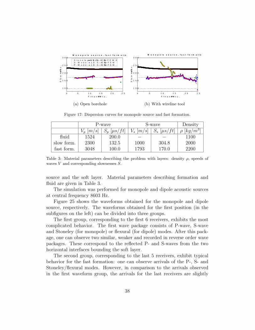
The remaining examples are presented in Appendix Appendix B: withthe monopole point source at frequency 50 Hz for both formulations (Fig-ures B.37, B.38, B.40 and B.39). and 25 kHz for both formulations (Fig-ures B.41, B.42, B.44 and B.43), with the dipole source at frequency 50 Hzfor formulation B (B.45, B.46, B.48 and B.47) and 10 kHz (Figures B.50 andB.49).

Similar observations to those for pure acoustic problem can be made: thehp algorithm produces different meshes for low and high frequencies. Theconvergence rate is at least algebraic (Figures 11, 12, 13, 14). For all testedcases the PML efficiently damps the solution to the machine zero value andthus enables to accurately solve the elastic wave propagation problem for thehomogenous elastic material for the range of frequencies from 50 Hz to 25kHz.

29

(a) Fine mesh (b) Re(ur), Re(uz) and Re(utheta)along the profile (zoomed in PML zone,PML marked in blue)

Figure 9: Elasticity. Dipole point source. Formulation A. f = 10 kHz

30

(a) Re(ur) (b) Re(uz) (c) Re(uθ)

(d) log∣∣ufr − uexr ∣∣ (e) log

∣∣ufz − uexz ∣∣ (f) log |uθf − uθex |

Figure 10: Elasticity. Dipole point source. Formulation A. f = 10 kHz

31

1 0 3 1 0 4 1 0 5

1 E - 3

0 . 0 1

0 . 1

1

1 0

1 0 0

Relat

ive en

ergy e

rror, %

# D O F S



(a) Formulation A

1 0 3 1 0 4 1 0 5

1 E - 3

0 . 0 1

0 . 1

1

1 0

1 0 0

Relat

ive en

ergy e

rror, %

# D O F S



(b) Formulation B

Figure 11: Convergence for elasticity. Monopole point source. f = 50 Hz

1 0 4 1 0 51 E - 3

0 . 0 1

0 . 1

1

1 0

Relat

ive en

ergy e

rror, %

# D O F S



(a) Formulation A

1 0 4 1 0 51 E - 3

0 . 0 1

0 . 1

1

1 0

Re

lative

energ

y erro

r, %

# D O F S



(b) Formulation B

Figure 12: Convergence for elasticity. Monopole point source. f = 25 kHz

4.4. Coupled case

Verification of the code for the coupled case was performed using anotherapproach. For the purpose of comparison, instead of using an analytical solu-tion, we used another 1D semi-analytical code [29] which calculates solutionsfor simple geometries according to the mathematical procedure described in[11, 12]. As an alternate to the comparison of pressure and displacementwithin the computational domain, we chose to compare the waveforms anddispersion curves obtained by postprocessing the direct results of the simula-tions for the whole range of frequencies. The approach enables to verify thecomplete method (i.e. simulation of the problem for the whole range of fre-quencies and the transformation of the solution into the time domain using

32

1 0 3 1 0 4 1 0 5

1 E - 3

0 . 0 1

0 . 1

1

1 0

1 0 0

Relat

ive en

ergy e

rror, %

# D O F S



(a) Formulation A

1 0 3 1 0 4 1 0 5

1 E - 3

0 . 0 1

0 . 1

1

1 0

1 0 0

Relat

ive en

ergy e

rror, %

# D O F S



(b) Formulation B

Figure 13: Convergence for elasticity. Dipole point source. f = 50 Hz

1 0 4 1 0 51 E - 4

1 E - 3

0 . 0 1

0 . 1

1

1 0

Relat

ive en

ergy e

rror, %

# D O F S



(a) Formulation A

1 0 4 1 0 5

1 E - 3

0 . 0 1

0 . 1

1

1 0

Re

lative

energ

y erro

r, %

# D O F S



(b) Formulation B

Figure 14: Convergence for elasticity. Dipole point source. f = 10 kHz

fast inverse Fourier transform) and, additionally, gives a physical verificationof the method by clear exposition of the different kinds of waves that aregenerated in the formation and the borehole.

We considered two geometrical cases: with open borehole (Figure 15(a)),and the presence of the solid elastic wireline tool, centered in the borehole(Figure 15(b)). Inside the borehole we put the acoustic source and the arrayof 8 equally spaced receivers (spacing equal 0.15 m). The simulations wereperformed for fast and slow homogeneous formations. Physical parametersfor the materials used in the calculations are summarized in Table 2. Inall cases we set quality factors to ∞, i.e. we assume no attenuation in thematerials. We considered two kinds of acoustic sources: monopole and dipolesource, both being Ricker wavelets with a central frequency of 8603 Hz.

33

r

z

PML

PML

PML

0.102

0.108

1.0

3.0

1.05

0.45

8x

FLUID FORMATION

0.25

(a) Open borehole

r

z

PML

PML

PML

0.1020.108

1.0

3.0

1.05

0.45

8x

FLU

ID

FORMATION

TOO

L

0.045

0.25

(b) With the solid wireline tool

Figure 15: Geometries for the coupled problems. All the dimensions in meters.

The first example deals with the modeling of a homogeneous fast for-mation for a monopole source at central frequency 8603 Hz. The obtainedwaveforms are presented in Figure 16. The thick curves are obtained from 1Dsemianalytical code, whilst the thin ones are coming from the hp-adaptiveFEM calculations. In both cases: without a tool (subfigure (a)) and in pres-ence of the tool (subfigure (b)), we can easily identify S-wave (indicated byS ) and Stoneley wave package (indicated by St) arrivals, respectively. TheP-wave mode, although present (see the dispersion curves in Figure 17a), isnot clearly visible because its amplitude is very small in comparison to theStoneley mode. Due to the amplitude comparison, most of the wave energy

34

P-wave S-wave DensityVp [m/s] 1/Vp [µs/ft] Vs [m/s] 1/Vs [µs/ft] ρ [kg/m3]

fluid 1524 200.0 − − 1100fast form. 3048 100.0 1793 170.0 2200slow form. 2300 132.5 1000 304.8 2000

tool 5860 52.0 3130 97.4 7800

Table 2: Material parameters used in verification of the code for coupled problems.

is carried by the dominant Stoneley mode. In the presence of the tool how-ever, we are also able to identify a very weak mode which is a superpositionof the tool S-wave (indicated by TS ) and the formation P-wave. Anothernoticeable change between these two cases is the variation in a shape of theStoneley mode, but not in the time arrival of this mode.

Comparison of the dispersion curves obtained for both cases (Figure 17)also confirms existence of the mentioned modes. This kind of presentationof the existing modes gives a direct insight into the nature of the modesand makes possible to instantly estimate the slowness and character of themodes, which is of a primary importance for recovering information aboutelastic parameters of the formation. Thus we see, for the whole range offrequencies, the slowest, weakly dispersive Stoneley mode which additionallyexhibits anomalous dispersivity (dispersion curve has negative slope). Themode is characteristic for the fast formation.

The following (pink) dispersive mode is the pseudo-Rayleigh mode. Itbegins at the cutoff frequency and drops from formation S-wave velocity toapproach the fluid wave speed at high frequencies. Very weak formationP-wave mode is seen for the case without the tool (subfigure (a)). In thepresence of the tool, a corresponding tool mode (orange-pink) appears insubfigure (b).

The second example deals with the modeling of a homogeneous slow for-mation for a monopole source at central frequency 8603 Hz. The waveformsare presented in Figure 18. In both cases (without a tool — subfigure (a),and with the tool — subfigure (b)), we can easily identify P-wave (indicatedby P) and Stoneley wave packages (indicated by St) arrivals, respectively.Obviously, the time arrivals of the wave packages are delayed in comparisonto the fast formation. Lack of the S-wave agrees with the theory: in theslow formation, S-wave velocity falls below the speed of sound in the bore-hole fluid, and thus refraction of the shear head wave is impossible. In the

35

presence of the tool however, an additional tool mode (indicated by TP)introduces some disturbance into the formation P-wave arrival.

The corresponding dispersion plots (Figure 19)) clearly identify the actualmodes. As for the fast formation, the Stoneley mode is dominant. The modeis weakly dispersive at higher frequencies and it exhibits a larger dispersivityat the low frequency limit. The P-wave mode is clearly visible in both cases,and so is the tool mode in the case with the tool present.

The next example deals with the modeling of a homogeneous fast for-mation for a dipole source at central frequency 8603 Hz. The waveformsare presented in Figure 20. For both cases, one can identify arrivals of theS-wave and highly dispersive flexural wave packages (indicated by F ). In thepresence of the tool (subfigure (b)), an additional, perturbed by the tool,formation P-wave arrival can be observed. The dispersion plot (Figure 21a)for the open borehole indicates existence of the first two flexural modes (the1st in yellow, and the 2nd in blue/red). The important feature of the flexuralmodes is that its phase velocity drops from the formation S-wave velocity atthe cutoff frequency, which makes this type of sonic measurement a usefultool in estimating elastic parameters of the formation. In the presence of thetool, an additional tool mode is present (Figure 21b).

The last example focuses on the modeling of a homogeneous slow for-mation for a dipole source at central frequency 8603 Hz. The waveforms arepresented in Figure 22. For both cases one can identify arrivals of the P-waveand flexural wave packages. In the presence of the tool (subfigure (b)), theP-wave package is perturbed by the tool modes. The dispersion plot (Fig-ure 23a) for the open borehole indicates existence of the first flexural modes(yellow) and the P-wave mode (red). The flexural mode begins at S-wavespeed at low frequencies which makes possible to pick up the formation S-wave slowness despite the fact that the formation S-wave is not observed inwaveforms. In the presence of the tool, an additional tool mode is observed(Figure 23b).

In all the presented cases, the dispersion curves and waveforms, calculatedvia postprocessing solutions from the hp simulations, perfectly match theresults obtained with the 1D semi-analytical method. This confirms the highaccuracy of the hp elements and builds up the confidence in the method.

36

0 . 0 0 . 5 1 . 0 1 . 5 2 . 0 2 . 5 3 . 0 3 . 5 4 . 0

3

4

P S

1 D : R X 1 R X 2 R X 3 R X 4 R X 5 R X 6 R X 7 R X 82 D : R X 1 R X 2 R X 3 R X 4 R X 5 R X 6 R X 7 R X 8

Norm

alized

pres

sure,

rece

ivers

offse

t, m

T i m e , m s

S t

(a) Open borehole

0 . 0 0 . 5 1 . 0 1 . 5 2 . 0 2 . 5 3 . 0 3 . 5 4 . 0

3

4

S S t


Norm

alized

pres

sure,

rece

ivers

offse

t, m

T i m e , m s

T S

(b) With wireline tool

Figure 16: Waveforms for monopole source and fast formation.

5. Representative examples

5.1. Fast formation with a soft layer

The geometry of the first nontrivial example is shown in Figure 24. Out-side of the open borehole, and within the the fast formation, there is a softlayer of thickness 0.5 m. The radial thickness of the formation, excluding thePML layer, is equal 25 cm.

We consider two positions of the array of 13 receivers: the first (leftsubfigure), where the array is facing the soft layer and the second (rightsubfigure), where the array of receivers is placed in between the acoustic

37

0 5 1 0 1 5 2 0 2 5

1 0 0

1 5 0

2 0 0

2 5 0

3 0 0S t o n e l e y m o d e : 1 D S - A 2 D h p - F E M AS - M o d e : 1 D S - A 2 D h p - F E MP - M o d e : 1 D S - A 2 D h p - F E M

M o n o p o l e s o u r c e , f a s t f o r m a t i o n , o p e n b o r e h o l e

Slown

ess,

us/ft

F r e q u e n c y , k H z

(a) Open borehole

0 5 1 0 1 5 2 0 2 5

1 0 0

1 5 0

2 0 0

2 5 0

3 0 0M o n o p o l e s o u r c e , f a s t f o r m a t i o n w i t h t o o l

Slown

ess,

us/ft



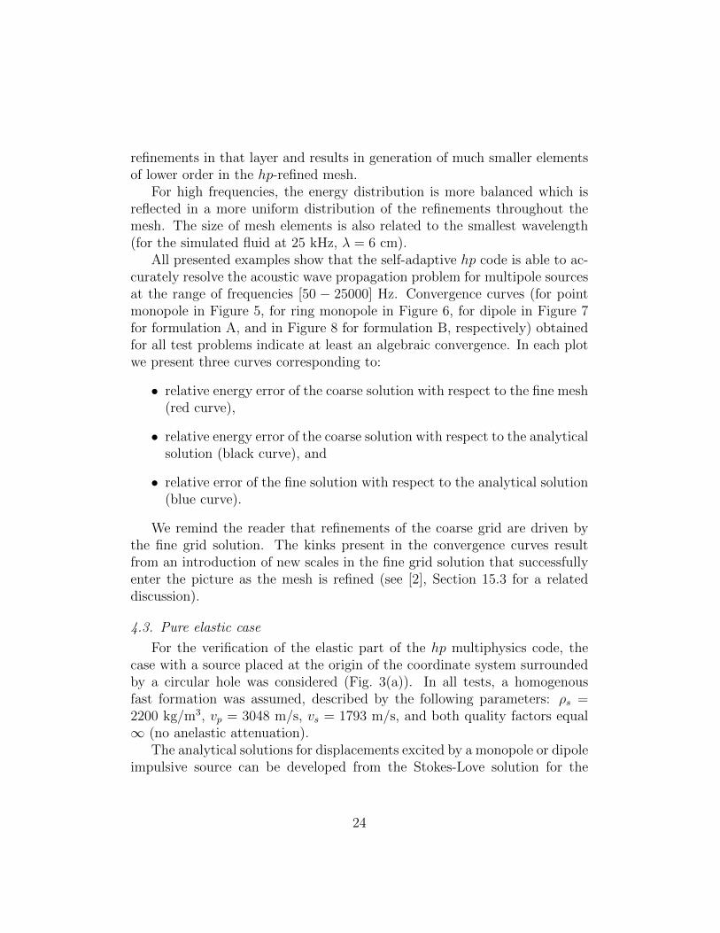
Figure 17: Dispersion curves for monopole source and fast formation.

P-wave S-wave DensityVp [m/s] Sp [µs/ft] Vs [m/s] Ss [µs/ft] ρ [kg/m3]

fluid 1524 200.0 − − 1100slow form. 2300 132.5 1000 304.8 2000fast form. 3048 100.0 1793 170.0 2200

Table 3: Material parameters describing the problem with layers: density ρ, speeds ofwaves V and corresponding slownesses S.

source and the soft layer. Material parameters describing formation andfluid are given in Table 3.

The simulation was performed for monopole and dipole acoustic sourcesat central frequency 8603 Hz.

Figure 25 shows the waveforms obtained for the monopole and dipolesource, respectively. The waveforms obtained for the first position (in thesubfigures on the left) can be divided into three groups.

The first group, corresponding to the first 6 receivers, exhibits the mostcomplicated behavior. The first wave package consists of P-wave, S-waveand Stoneley (for monopole) or flexural (for dipole) modes. After this pack-age, one can observe two similar, weaker and recorded in reverse order wavepackages. These correspond to the reflected P- and S-waves from the twohorizontal interfaces bounding the soft layer.

The second group, corresponding to the last 5 receivers, exhibit typicalbehavior for the fast formation: one can observe arrivals of the P-, S- andStoneley/flexural modes. However, in comparison to the arrivals observedin the first waveform group, the arrivals for the last receivers are slightly

38

0 . 0 0 . 5 1 . 0 1 . 5 2 . 0 2 . 5 3 . 0 3 . 5 4 . 0 4 . 5 5 . 0 5 . 5

3

4

S t


Norm

alized

pres

sure,

rece

ivers

offse

t, m

T i m e , m s

P

(a) Open borehole

0 . 0 0 . 5 1 . 0 1 . 5 2 . 0 2 . 5 3 . 0 3 . 5 4 . 0 4 . 5 5 . 0 5 . 5

3

4

T P S t


Norm

alized

pres

sure,

rece

ivers

offse

t, m

T i m e , m s

P


Figure 18: Waveforms for monopole source and slow formation.

delayed due to the presence of the slow formation layer. After the main wavepackage, one can observe very weak, additional waves. These are multiplyreflected (trapped in the soft layer) waves.

The third group of waveforms, corresponds to the central receivers, facingdirectly the soft layer. In here one can clearly discriminate only fast formationP-wave arrivals.

The waveforms obtained for the second position (subfigures on the right)exhibits a similar behavior. Analogously to the first group of waveforms forthe position 1, we one can observe arrivals of the direct P-, S- and Stone-ley/flexural modes, followed by two packages of the reflected waves.

39

0 5 1 0 1 5 2 0 2 5

1 0 0

2 0 0

3 0 0

4 0 0M o n o p o l e s o u r c e , s l o w f o r m a t i o n , o p e n b o r e h o l e

S t o n e l e y m o d e : 1 D s e m i - a n a l y t i c a l 2 D h p - F E M A n a l y t i c a l2 n d M o d e : 1 D s e m i - a n a l y t i c a l 2 D h p - F E M3 r d M o d e : 1 D s e m i - a n a l y t i c a l 2 D h p - F E M

Slown

ess,

us/ft


(a) Open borehole

0 5 1 0 1 5 2 0 2 5

1 0 0

2 0 0

3 0 0

4 0 0M o n o p o l e s o u r c e , s l o w f o r m a t i o n w i t h t o o l

S t o n e l e y m o d e : 1 D s e m i - a n a l y t i c a l 2 D h p - F E MM a n d r e l m o d e : 1 D s e m i - a n a l y t i c a l 2 D h p - F E MP - w a v e : 1 D s e m i - a n a l y t i c a l 2 D h p - F E M

Slown

ess,

us/ft



Figure 19: Dispersion curves for monopole source and slow formation.

Figure 26 shows the results of the dispersion processing, obtained for themonopole and dipole source, respectively. Left subfigures displays curvescalculated for the position 1. In that case, it is nearly impossible to recoverany meaningful information about the physical parameters of the formationdue to the superposition of the direct and multiply reflected waves. Theextended Prony method, used for dispersion processing, is unable to detectthe existing modes, when different subsets of receivers collect data containingdifferent acoustic modes.

On the other hand, the dispersion processing is successful in the secondcase where all the receivers obtain a similar information.

In the case of the monopole acoustic source, one can identify the slowestStoneley mode (with characteristic for the fast formation anomalous disper-sivity) and the pseudo-Rayleigh mode (beginning slightly above the S-waveslowness S3 of the fast formation). One can also observe highly dispersivemodes (vertical lines) which corresponds to the reflected waves.

Similarly, for the dipole case, one can also identify the first and the secondflexural modes, both of them beginning slightly above the S-wave slownessS3 of the fast formation. The curves corresponding to the reflected waves arepresent in this case as well.

5.2. Logging while drilling

The next example deals with the simulation of the sonic logging-while-drilling (LWD) scenarios for the homogeneous fast and slow formations. Incomparison to the wireline tool, which is modeled as a solid cylinder occu-pying a part of the borehole, the LWD tool possesses an internal fluid filled

40

0 . 0 0 . 5 1 . 0 1 . 5 2 . 0 2 . 5 3 . 0 3 . 5 4 . 0

3

4

F

Norm

alized

pres

sure,

rece

ivers

offse

t, m

T i m e , m s


S

(a) Open borehole

0 . 0 0 . 5 1 . 0 1 . 5 2 . 0 2 . 5 3 . 0 3 . 5 4 . 0

3

4

FP


Norm

alized

pres

sure,

rece

ivers

offse

t, m

T i m e , m s

S


Figure 20: Waveforms for dipole source and fast formation.

channel and occupies a much larger portion of the borehole. The smaller an-nulus filled with the fluid, as well as the additional vertical fluid filled channelchanges significantly the wave propagation environment.

The geometry for the problem is shown in Figure 27. Material parametersdescribing two kinds of formations and fluids are given in Table 4. In thecase of the monopole source, we used excitation at central frequency equal8000 kHz. For the dipole and quadrupole acoustic source, we used excitationat central frequency equal 3500 kHz.

Figure 28 shows the waveforms obtained for the fast and slow formation,respectively. In each case, we present the results obtained for a monopole,

41

0 5 1 0 1 5 2 0 2 5

1 0 0

2 0 0

3 0 01 s t F l e x u r a l m o d e : 1 D s e m i - a n a l y t i c a l 2 D h p - F E M A n a l y t i c a l2 n d F l e x u r a l m o d e : 1 D s e m i - a n a l y t i c a l 2 D h p - F E M

Slown

ess,

us/ft


D i p o l e s o u r c e , f a s t f o r m a t i o n , n o t o o l

(a) Open borehole

0 5 1 0 1 5 2 0 2 5

1 0 0

2 0 0

3 0 0 F l e x u r a l m o d e : A n a l y t i c a l1 D s e m i - a n a l y t i c a l 2 D h p - F E M1 D s e m i - a n a l y t i c a l 2 D h p - F E M1 D s e m i - a n a l y t i c a l 2 D h p - F E M

Slown

ess,

us/ft


D i p o l e s o u r c e , f a s t f o r m a t i o n w i t h t o o l


Figure 21: Dispersion curves for dipole source and fast formation.

Id P-wave S-wave DensityVp [m/s] Sp [µs/ft] Vs [m/s] Ss [µs/ft] ρ [kg/m3]

tool 1 5862 52.0 2519 121.0 7800slow form. 2 2300 132.5 1000 304.8 2000fast form. 2 3048 100.0 1793 170.0 2200

fluid 3 1500 203.2 − − 1100

Table 4: Material parameters describing the LWD problems: density ρ, speeds of wavesV and corresponding slowness S.

dipole and quadrupole acoustic sources.For the monopole source, the first wave to arrive is a collar wave. For the

fast formation, it is weaker and simpler in shape. For the soft formation, thewave is more prominent and more complicated in shape due to the superpo-sition of stronger formation P-wave waveforms. In the fast formation, onecan further observe a weak, but distinguishable, arrival of formation S-wavepackage, followed by the strongest Stoneley mode. In the slow formation,the Stoneley mode can be observed as the last and the strongest waveformcomponent. It is also delayed, when compared with the fast formation.

For the dipole source and the fast formation, one can see only the arrivalof the dispersive formation flexural mode. The waveforms obtained for theslow formation are clearly separated into two groups: a highly dispersivecollar mode, followed by the formation flexural mode.

In the case of a quadrupole acoustic source, for both fast and slow for-mations, one can observe only one wave package which corresponds to theformation quadrupole (screw) mode. The arrival time of this mode corre-

42

0 . 0 0 . 5 1 . 0 1 . 5 2 . 0 2 . 5 3 . 0 3 . 5 4 . 0 4 . 5 5 . 0 5 . 5

3

4

5

F


No

rmaliz

ed pr

essu

re, re

ceive

rs off

set, m

T i m e , m s

P

(a) Open borehole

0 . 0 0 . 5 1 . 0 1 . 5 2 . 0 2 . 5 3 . 0 3 . 5 4 . 0 4 . 5 5 . 0 5 . 5

3

4

5

S T F


Norm

alized

pres

sure,

rece

ivers

offse

t, m

T i m e , m s

P


Figure 22: Waveforms for dipole source and slow formation.

sponds to the anticipated formation S-wave arrival.Figure 29 show the results of the dispersion processing, obtained for the

fast and the slow formations, respectively. In each case, we present the resultsobtained for a monopole, dipole and quadrupole acoustic source.

Comparing dispersion curves obtained for a monopole acoustic source,one can see a similar character of some curves. The topmost, slightly drop-ping curves, existing for all the frequencies, correspond to the formationStoneley mode. The Stoneley mode in the slow formation propagates with alower velocity. The second, deflecting curve, which exhibit exactly the samecharacter for both formations, corresponds to the collar monopole mode. In

43

0 5 1 0 1 5 2 0 2 51 0 0

2 0 0

3 0 0

4 0 0

D i o p o l e s o u r c e , s l o w f o r m a t i o n , o p e n b o r e h o l e

F l e x u r a l m o d e : 1 D S e m i - a n a l y t i c a l 2 D h p - F E M A n a l .P - w a v e : 1 D S e m i - a n a l y t i c a l 2 D h p - F E MSlo

wnes

s, us

/ft


(a) Open borehole

0 5 1 0 1 5 2 0 2 51 0 0

2 0 0

3 0 0

4 0 0

D i o p o l e s o u r c e , s l o w f o r m a t i o n w i t h t o o l

F l e x u r a l m o d e : 1 D S e m i - a n a l y t i c a l 2 D h p - F E M A n a l .M a n d r e l m o d e : 1 D S e m i - a n a l y t i c a l 2 D h p - F E MP - w a v e : 1 D S e m i - a n a l y t i c a l 2 D h p - F E M

Slown

ess,

us/ft



Figure 23: Dispersion curves for dipole source and slow formation.

addition, for the fast formation, one can clearly identify the nondispersiveS-wave curve.

In the case of the dipole acoustic source, the situation is more complicated.The reason for it is that the curve corresponding to the first flexural modecrosses with highly dispersive collar mode at a low frequency (c.a. 1 kHz)and thus produces a complex wave behavior in low frequencies. Here, thedispersion processing software was not able to discriminate these two curves:instead having two crossing curves, one ended up with two separate curveswith some lag between them. Each of the curves is composed of fragmentsof flexural and collar curves. For the case of the fast formation, a separatecurve corresponding to the formation S-wave mode is present. In the case ofthe slow formation, picking up the formation S-wave slowness is impossible,due to the lack of the low frequency part of the 1st flexural mode.

Such a problem does not occur for the quadrupole acoustic source. Thequadrupole collar mode is well separated from the formation screw mode,because the collar mode begins at some cut-off frequency, which is beyondthe excitation frequency range of the source. Thus, one can clearly identifythe dispersive formation quadrupole mode, which begins at formation S-waveslowness at low frequency. For the fast formation, the independent S-wavemode exists, manifesting itself in an additional dispersion curve.

6. Conclusions

A summary. The paper is a continuation of [1] and focuses on extending thefully automatic hp FE methods to coupled acoustic/anelasticity problems.The methodology is applied to a challenging problem of modeling sonic tools

44

r

z

PMLPM

L

PML

0.1020.108

0.25

3.0

0.70

1.05

13x

FLUID

FAST FORM.

FAST FORM.

SLOW FORM.0.5

0.75

r

z

PML

PML

PML

0.1020.108

0.25

3.0

0.25

0.30

13x

FLUID

FAST FORM.

FAST FORM.

SLOW FORM.0.5

1.95

Figure 24: Geometry of the problem with soft layer. Two positions of the array of receivers.

45

1 2 3 4 52 . 0

2 . 5

3 . 0

3 . 5

4 . 0

4 . 5

5 . 0

Norm

alized

pres

sure,

rece

ivers

offse

t, m

T i m e , m s

(a) Monopole, position 1

1 2 3 4 5 62 . 5

3 . 0

3 . 5

4 . 0

4 . 5

5 . 0

5 . 5

Norm

alized

pres

sure,

rece

ivers

offse

t, m

T i m e , m s

(b) Dipole, position 1

1 2 3 4 5 6 7 8

2 . 5

3 . 0

3 . 5

4 . 0

4 . 5

5 . 0

Norm

alized

pres

sure,

rece

ivers

offse

t, m

T i m e , m s

(c) Monopole, position 2

1 2 3 4 5 6 7 8 92 . 5

3 . 0

3 . 5

4 . 0

4 . 5

5 . 0

5 . 5

Norm

alized

pres

sure,

rece

ivers

offse

t, m

T i m e , m s

(d) Dipole, position 2

Figure 25: Problem with layers: waveforms for the monopole and dipole source.

in the borehole environment. The extension of adaptive hp-algorithm tocoupled problems required an automatic energy rescaling procedure. Themethod delivers a superior accuracy compared with non-adaptive discretiza-tion schemes (including Finite Differences) and we have documented theclaim with a careful verification of the methodology and the code. Finally,we have presented a number of non-trivial examples illustrating the potentialof the hp-technology.

Challenges and future work. It would be a lie to claim that we have notencountered any problems. The main challenge comes from the constructionof Perfectly Matched Layer and its mathematical understanding. The PMLmethod is practically the only technique that we can think of in the case ofgeometries involving multiple layers and the borehole. The construction ofthe implemented PML extrapolates heavily from a simple 1D case and seemsto be insufficient in the case of waveguide geometries, especially in contextof coupled problems and anisotropies [30]. We have not experienced theseproblems in the examples presented in this paper.

Our current work is marching in two directions. Non-axisymmetric ge-

46

5 10 15 20 2550

100

150

200

250

300

350

400

P1

P2

S2

P3

S3

Dispersion curves

Frequency, kHz

Slo

wne

ss, µ

s/ft

(a) Monopole, position 1

5 10 15 20 2550

100

150

200

250

300

350

400

P1

P2

S2

P3

S3

Dispersion curves

Frequency, kHz

Slo

wne

ss, µ

s/ft

(b) Dipole, position 1

5 10 15 20 2550

100

150

200

250

300

350

400

P1

P2

S2

P3

S3

Dispersion curves

Frequency, kHz

Slo

wne

ss, µ

s/ft

(c) Monopole, position 2

5 10 15 20 2550

100

150

200

250

300

350

400

P1

P2

S2

P3

S3

Dispersion curves

Frequency, kHz

Slo

wne

ss, µ

s/ft

(d) Dipole, position 2

Figure 26: Problem with layers: dispersion curves for the monopole source.

ometries call for the use of 3D elements and the 3D implementation is indeedunderway. On the modeling side, we focus on more sophisticated models forthe formation including various poroelasticity theories. We hope to reportnew results soon in a forthcoming paper.

Appendix A. Verification of the acoustic part of the code

47

r

PML

FORMATION

z

0.0254

0.10795

0.5

1.52

41.

524

0.25

11x

FLU

ID

0.1

0.0872

TOO

L

Figure 27: Geometry of the LWD problem.

48

0 1 2 3 4 51

1.5

2

2.5

3

3.5

P1

S1

P2

S2

P3

Waveforms

Time, ms

Am

plitu

de /

offs

et, m

(a) Fast formation, monopole

0 1 2 3 4 51

1.5

2

2.5

3

3.5

P1

S1

P2

S2

P3

Waveforms

Time, ms

Am

plitu

de /

offs

et, m

(b) Slow formation, monopole

0 1 2 3 4 51

1.5

2

2.5

3

3.5

P1

S1

P2

S2

P3

Waveforms

Time, ms

Am

plitu

de /

offs

et, m

(c) Fast formation, dipole

0 1 2 3 4 51

1.5

2

2.5

3

3.5

P1

S1

P2

S2

P3

Waveforms

Time, ms

Am

plitu

de /

offs

et, m

(d) Slow formation, dipole

0 1 2 3 4 51

1.5

2

2.5

3

3.5

P1

S1

P2

S2

P3

Waveforms

Time, ms

Am

plitu

de /

offs

et, m

(e) Fast formation, quadrupole

0 1 2 3 4 51

1.5

2

2.5

3

3.5

P1

S1

P2

S2

P3

Waveforms

Time, ms

Am

plitu

de /

offs

et, m

(f) Slow formation, quadrupole

Figure 28: Waveforms obtained for LWD problem with homogeneous fast formation anddifferent acoustic sources. P and S with indices (see Table 4) indicate appropriate arrivalsof P - and S-waves.

49

5 10 15 20 25

100

200

300

400

P1

S1

P2

S2

P3

Dispersion curves

Frequency, kHz

Slo

wne

ss, µ

s/ft

(a) Fast formation, monopole

5 10 15 20 25

100

200

300

400

P1

S1

P2

S2

P3

Dispersion curves

Frequency, kHz

Slo

wne

ss, µ

s/ft

(b) Slow formation, monopole

2 4 6 8 10

100

200

300

400

P1

S1

P2

S2

P3

Dispersion curves

Frequency, kHz

Slo

wne

ss, µ

s/ft

(c) Fast formation, dipole

2 4 6 8 10

100

200

300

400

P1

S1

P2

S2

P3

Dispersion curves

Frequency, kHz

Slo

wne

ss, µ

s/ft

(d) Slow formation, dipole

2 4 6 8 10

100

200

300

400

P1

S1

P2

S2

P3

Dispersion curves

Frequency, kHz

Slo

wne

ss, µ

s/ft

(e) Fast formation, quadrupole

2 4 6 8 10

100

200

300

400

P1

S1

P2

S2

P3

Dispersion curves

Frequency, kHz

Slo

wne

ss, µ

s/ft

(f) Slow formation, quadrupole

Figure 29: Dispersion curves obtained for LWD problem with homogeneous fast formationand different acoustic sources. P and S with indices (see Table 4) indicate appropriatearrivals of P - and S-waves.

50



Figure A.30: Acoustics. Monopole point source. Formulation A. f = 50 Hz

51



Figure A.31: Acoustics. Monopole point source. Formulation A. f = 25 kHz

52



Figure A.32: Acoustics. Ring source. Formulation A. f = 50 Hz

53



Figure A.33: Acoustics. Ring source. Formulation A. f = 25 kHz

54



Figure A.34: Acoustics. Dipole point source. Formulation A. f = 50 Hz

55



Figure A.35: Acoustics. Dipole point source. Formulation B. f = 50 Hz

56



Figure A.36: Acoustics. Dipole point source. Formulation B. f = 25 kHz

57

Appendix B. Verification of the elastic part of the code

58

(a) Re(ur) (b) Re(uz)

(c) log∣∣ufr − uexr ∣∣ (d) log

∣∣ufz − uexz ∣∣Figure B.37: Elasticity. Monopole point source. Formulation A. f = 50Hz

59

(a) Fine mesh (b) Re(ur) (red) and Re(uz) (blue) alongthe profile (zoomed in PML zone, PMLmarked in blue)

Figure B.38: Elasticity. Monopole point source. Formulation A. f = 50Hz


Figure B.39: Elasticity. Monopole point source. Formulation B. f = 50Hz

60



∣∣ufz − uexz ∣∣Figure B.40: Elasticity. Monopole point source. Formulation B. f = 50Hz

61



∣∣ufz − uexz ∣∣Figure B.41: Elasticity. Monopole point source. Formulation A. f = 25kHz

62


Figure B.42: Elasticity. Monopole point source. Formulation A. f = 25kHz


Figure B.43: Elasticity. Monopole point source. Formulation B. f = 25kHz

63



∣∣ufz − uexz ∣∣Figure B.44: Elasticity. Monopole point source. Formulation B. f = 25kHz

64



∣∣ufz − uexz ∣∣ (f) log∣∣∣ufθ − uexθ ∣∣∣

Figure B.45: Elasticity. Dipole point source. Formulation A. f = 50Hz

65


Figure B.46: Elasticity. Dipole point source. Formulation A. f = 50Hz


Figure B.47: Elasticity. Dipole point source. Formulation B. f = 50Hz

66




Figure B.48: Elasticity. Dipole point source. Formulation B. f = 50Hz

67


Figure B.49: Elasticity. Dipole point source. Formulation B. f = 10kHz

68




Figure B.50: Elasticity. Dipole point source. Formulation B. f = 10kHz

69

[1] C. Michler, L. Demkowicz, C. Torres-Verdin, Numerical simulation ofborehole acoustic logging in the frequency and time domains with hp-adaptive finite elements, Comput. Methods Appl. Mech. Engrg. 198(2009) 1821–1838.

[2] L. Demkowicz, Computing with hp Finite Elements. I.One- and Two-Dimensional Elliptic and Maxwell Problems, Chapman & Hall/CRCPress, Taylor and Francis, 2006.

[3] L. Demkowicz, J. Kurtz, D. Pardo, M. Paszynski, W. Rachowicz,A. Zdunek, Computing with hp Finite Elements. II. Frontiers: Three-Dimensional Elliptic and Maxwell Problems with Applications, Chap-man & Hall/CRC, 2007.

[4] L. Demkowicz, J. Kurtz, An hp framework for coupled multiphysicsproblems, Tech. rep., ICES, in preparation (2010).

[5] H. Sanchez, E. Sanchez Palencia, Vibration and Coupling of ContinuousSystems: Asymptotic Methods, Springer-Verlag, 1989.

[6] J. Oden, L. Demkowicz, Applied Functional Analysis for Science andEngineering, Chapman & Hall/CRC Press, Boca Raton, 2010, secondedition.

[7] L. Demkowicz, Asymptotic convergence in finite and boundary elementmethods. Part 1: Theoretical results, Computers & Mathematics withApplications 27 (12) (1994) 69–84.

[8] L. Demkowicz, Asymptotic convergence in finite and boundary elementmethods. Part 2: The lbb constant for rigid and elastic problems, Com-puters & Mathematics with Applications 28 (6) (1994) 93–109.

[9] G. Gatica, A. Marquez, S. Meddahi, Analysis of the coupling of primaland dual-mixed finite element methods for a two-dimensional fluid –solid interaction problem, SIAM J. Numer. Anal. 45 (2007) 2072–2097.

[10] J. White, Underground Sound. Application of seismic waves., Vol. 18 ofMethods in Geochemistry and Geophysics, Elsevier, 1983.

[11] F. L. Paillet, C. H. Cheng, Acoustic Waves in Boreholes, CRC Press,1991.

70

[12] X.-M. Tang, A. Cheng, Quantitative Borehole Acoustic Methods, Vol. 24of Handbook of Geophysical Exploration. Seismic Exploration., Elsevier,2004.

[13] K. Bhasavanija, L. M. Nicoletis, T. K. Young, A finite difference model ofan acoustic logging tool: the borehole in a horizontally layered gelogicmedium, presented at the 52nd Ann. Mtg. and Expos. Soc. Explor.Geophys., , Dallas, 312–313 (1982).

[14] R. Stephen, F. Cardo-Casas, C. Cheng, Finite-difference syntheticacoustic logs, Geophysics 50 (10) (1985) 1588–1609.

[15] C. Randall, D. Scheibner, P. Wu, Multipole borehole acoustic wave-forms: synthetic logs with beds and borehole washouts, Geophysics56 (11) (1991) 1757–1769.

[16] H. Leslie, C. Randall, Multipole sources in boreholes penetratinganisotropic formations: Numerical and experimental results, J. Acoust.Soc. Amer. 91 (1) (1992) 12–27.

[17] N. Cheng, C. Cheng, M. Toksoz, Borehole wave propagation in threedimensions, J. Acoust. Soc. Amer. 97 (6) (1995) 3483–3493.

[18] T. Wang, X.-M. Tang, Finite-difference modeling of elastic wave prop-agation: a nonsplitting perfectly matched layer approach, Geophysics68 (5) (2003) 1749–1755.

[19] B. Sinha, E. Simsek, L. Q.-H., Elastic-wave propagation in deviatedwells in anisotropic formations, Geophysics 71 (6) (2003) D191–D202.

[20] S. Chang, Finite element modeling of borehole acoustics, J. Acoust. Soc.Amer. 69 (S1) (1981) S90–S90.

[21] M. Frehner, S. M. Schmalholz, Finite-element simulations of stoneleyguided-wave reflection and scattering at the tips of fluid-filled fractures,Geophysics 75(2) (2010) T23–T36.

[22] T. J. Chung, Applied Continuum Mechanics, Cambridge UniversityPress, 1996.

[23] J. Pujol, Elastic Wave Propagation and Generation in Seismology, Cam-bridge University Press, 2003.

71

[24] K. Aki, P. G. Richards, Quantitative Seismology, University ScienceBooks, 2002.

[25] G. A. Winbow, Compressional and shear arrivals in a multipole soniclog, Geophysics 50 (7) (1985) 1119–1126.

[26] J. H. Bramble, J. E. Pasciak, D. Trenev, Analysis of a finite PML ap-proximation for the three dimensional elastic wave scattering problem,Mathematics of Computation (in press).

[27] M. Tezer-Sesgin, S. Dost, On the fundamental solutions of the axisym-metric Helmholtz-type equations, Applied Mathematical Modelling 17(1993) 47–51.

[28] A. Ben-Menahem, S. J. Singh, Seismic Waves and Sources, Springer-Verlag, 1981.

[29] J. Ma, C. Torres-Verdin, Radial 1D simulation of multipole sonic wave-forms in the presence of a centered non-rigid cylindrical tool and trans-versely isotropic elastic formations, in: C. Torres-Verdin (Ed.), 8th An-nual Formation Evaluation Research Consortium Report, Center forPetroleum and Geosystems Enigineering. The University of Texas atAustin, 2008.

[30] E. Becache, S. Fauqueux, P. Joly, Stability of perfectly matched lay-ers, group velocities and anisotropic waves, Journal of ComputationalPhysics 188 (2003) 399–433.

72

solution of coupled acoustic-elastic wave propagation ... · solution of coupled acoustic-elastic...

Documents