solution of the diffusion equation - california state …lcaretto/me501b/diffusion.doc · web...

College of Engineering and Computer ScienceMechanical Engineering Department

Notes on Engineering AnalysisLarry Caretto January 22, 2009

Solution of the Diffusion Equation

Jacaranda (Engineering) 3333 Mail Code Phone: 818.677.6448E-mail: [email protected] 8348 Fax: 818.677.7062

mailto:[email protected]

Solution of the diffusion equation L. S. Caretto, January 22, 2009

Introduction and problem definition

The diffusion equation describes the diffusion of species or energy starting at an initial time, with an initial spatial distribution and progressing over time. The simplest example has one space dimension in addition to time. In this example, time, t, and distance, x, are the independent variables. The solution is obtained for t 0 and 0 x xmax. The dependent variable, species or temperature, is identified as u(x,t) in the equations below. The basic diffusion equation is written as follows.

[1]

Here, , is a species or thermal diffusion coefficient with dimensions of length squared over time. The initial condition specifies the value of u at all values of x at t = 0. This initial condition is usually written as follows:

u(x,0) = u0(x) [2]

The boundary conditions at x = 0 and x = xmax, can be functions of time in general. These are written as follows (with subscripts L and R denoting left and right).

u(0,t) = uL(t) u(xmax,t) = uR(t) [3]

There is actually a discontinuity in the initial conditions and the boundary conditions. The initial conditions are assumed to hold for all times less than or equal to zero. The boundary conditions hold for t > 0. This discontinuity only occurs at the boundaries. For example, the initial condition may be that u = 0 for all x and the boundary conditions may be that u = 100 at both boundaries for t > 0. This creates a discontinuity at t = 0 for x = 0 and x = xmax. Fortunately, this discontinuity does not affect our ability to solve the problem.

For the simplest cases we will consider both the initial and boundary conditions to be constant. However, in the most general case the boundary conditions may be given by any functional forms for u0(x). uL(t), and uR(t)

Basic solution process

The solution of the diffusion proceeds by a method known as the separation of variables. In this method we postulate a solution that is the product of two functions, T(t) a function of time only and X(x) a function of the distance x only. With this assumption, our solution becomes.

u(x,t) = X(x)T(t) [4]

We do not know, in advance, if this solution will work. However, we assume that it will and we substitute it for u in equation [1]. Since X(x) is a function of x only and T(t) is a function of t only, we obtain the following result when we substitute equation [4] into equation [1].


[5]

If we divide the final equation through by the product X(x)T(t), we obtain the following result.

[6]

The left hand side of equation [6] is a function of t only; the right hand side is a function of x only. The only way that this can be correct is if both sides equal a constant. This also shows that the separation of variables solution works. In order to simplify the solution, we choose the constant1 to be equal to2. This gives us two ordinary differential equations to solve.

[7]

The first equation becomes . The general solution to this equation is

known to be2 . The second differential equation in [7] can be written as

. The general solution to this equation is X(x) = Bsin(x) +

Ccos(x). Thus, our general solution for u(x,t) = X(x)T(t) becomes

[8]

We first consider a simple set of boundary conditions where u(0,t) = 0 and u(xmax,t) = 0. In order to satisfy these boundary conditions on u for all times, we have to have boundary conditions on X(x) that X(0) = X(xmax) = 0. With these homogenous boundary conditions on X(x) and the form of the original differential equation for X(x), the solution for X(x) is the solution of a Strum-Liouville problem. Accordingly, expect that we will be able to obtain an infinite set of solutions for X(x) that will give a complete set of orthogonal eigenfunctions.

If we substitute the boundary condition at x = 0 into equation [8], get the following result because sin(0) = 0 and cos(0) = 1.

1 The choice of –2 for the constant as opposed to just plain comes from experience. Choosing the constant to have this form now gives a more convenient result later. If we chose the constant to be simply , we would obtain the same result, but the expression of the constant would be awkward.2 As usual, you can confirm that this solution satisfies the differential equation by substituting the solution into the differential equation.


[9]

Equation [9] will be satisfied for all t if C2 = 0. With C2 = 0, we can apply the solution in equation [8] to the boundary condition at x = xmax.

[10]

Equation [10] can only be satisfied if the sine term is zero.3 This will be true only if xmax is an integral times . If n denotes an integer, we must have

[11]

We have an infinite number of solutions for X(x), as the integer n goes from 1 to infinity. We can write an individual solution as Xn(x) = sin(nx/xmax). Because the differential equation and boundary conditions for X(x), form a Sturm-Liouville problem, we know that the solutions to this problem, Xn(x), are an infinite set of orthogonal eigenfunctions. Since any integral value of n gives a solution to the original differential equations, with the boundary conditions that u = 0 at both boundaries, the most general solution is one that is a sum of all possible solutions, each multiplied by a different constant, Cn. This general solution is written as follows

[12]

We still have to satisfy the initial condition that u(x,0) = u0(x). Substituting this condition for t = 0 into equation [12] gives

[13]

Since the eigenfunctions sin(nx/xmax) are a complete set of orthogonal eigenfunctions in the interval x ≤ x ≤ xmax, we can expand any initial condition function, u0(x) in terms of these eigenfunctions. We can obtain the usual equation for eigenfunction expansion coefficients of Sturm-Liouville solutions by using the orthogonality relationships for integrals of the sine. If we multiply both sides of equation [13] by sin(mx/xmax), where m is another integer, and integrate both sides of the resulting equation from a lower limit of zero to an upper limit of xmax – the upper and lower limits of the Sturm-Liouville problem for X(x) – we get the following result.

3 Of course, the boundary condition is also satisfied if C1 = 0, but this gives u(x,t) = 0, not a very interesting solution.


[14]

In the second row of equation [14] we reverse the order of summation and integration because these operations commute. We then recognize that the integrals in the summation all vanish except for the one where n = m, because the eigenfunctions, sin(nx/xmax), are orthogonal. This leaves only one integral to evaluate. Solving for Cm and evaluating the last integral4 in equation [14] gives the following result.

[15]

For any initial condition, then, we can perform the integral on the right hand side of equation [15] to compute the values of Cm and substitute the result into equation [12] to compute u(x,t). We recognize that equation [15] is the usual equation for eigenfunction expansions in Sturm-Liouville problems.

As an example, consider the simplest case where u0(x) = U0, a constant. In this case we find Cm from the usual equation for the integral of sin(ax).

[16]

Since cos(m) is 1 when m is even and –1 when m is odd, the factor of 1 – cos(m) is zero when m is even and 2 when m is odd. This gives the final result for Cm shown below.

4 Using a standard integral table, and the fact that the sine of zero and the sine of an integral multiple of are zero, we find the following result:


[17]

Substituting this result into equation [12] gives the following solution to the diffusion equation when u0(x) = U0, a constant, and the boundary temperatures are zero.

[18]

If we substitute the equation for n into the summation terms we get the following result.

[19]

Equation [19] shows that the ratio u(x,t)/U0 depends on the dimensionless parameters t/(xmax)2 and x/xmax. Thus we can compute a universal plot of the solution as shown in Figure 1. Because the solution is symmetric about the midpoint x/L = 0.5, only the left half is plotted here.

Although we can obtain reasonable solutions using equation [19] for “large” times, we will not get a correct solution, within the limits of practical computers, if we try to evaluate equation [19] for times near zero. Figure 2 shows the results of using equation [19] to compute u(x,0)/U0 using various numbers of terms for t = 0. In this case we are trying to use the sine series to evaluate X(x) = 1. We see that taking more terms makes the solution more accurate away from x = 0, but no matter how many terms we take, there are still strong oscillations near x = 0. This result is well known and is called the Gibbs phenomena.

Nonzero boundary conditions

The use of zero boundary conditions to give us a Sturm-Liouville problem appears to be a major limitation on this approach. We can solve a broader class of problems, still using the same approach, by appropriate definitions of variables.


Figure 1 -- Diffusion Equation Solutionst = t/xmax

2

t = 0.0001

t = 0.

005

t = 0.

008

t = 0.01 t = 0.02

t = 0.03t = 0.04

t = 0.05

t = 0.08

t = 0.10

t = 0.125

t = 0.15

t = 0.175t = 0.2

t = 0.30

0

0.1

0.2

0.3

0.4

0.5

0.6

0.7

0.8

0.9

1

0 0.05 0.1 0.15 0.2 0.25 0.3 0.35 0.4 0.45 0.5x/L

u/U

Figure 2 -- Sine expansion for f(x) = 1

0

0.1

0.2

0.3

0.4

0.5

0.6

0.7

0.8

0.9

1

1.1

1.2

1.3

0 0.02 0.04 0.06 0.08 0.1 0.12 0.14 0.16 0.18 0.2

x

f(x) =

1

1 terms2 terms10 terms25 terms100 terms

First we consider the case were the boundary potentials, u(0,t) and u(xmax,t) are both set to a fixed value uB. In this case we can make the following simple variable transformation from u(x,t) to v(x,t).


v(x,t) = u(x,t) – uB [20]

This transformation gives v(0) = u(0,t) – uB = uB – uB = 0 and v(xmax) = u(xmax,t) – uB = uB – uB = 0. Thus, v has homogenous boundary conditions.

Since uB is a constant, when we substitute equation [20] into equation [1], we get the same equation in terms of v instead of u. Since the boundary conditions on v are that v = 0 at x = 0 and x = xmax, the differential equation for u is that of equation [1], and boundary conditions for v are the same as those used to derive the solution for u in equation [12]. Accordingly, equation [12] is the solution for v(x,t). When we apply the initial condition that u(x,0) = u0(x) to equation [12] for this revised problem, we get the following equation in place of equation [13].

[21]

Starting with this equation, we can repeat the derivation of equation [15] for Cm, which gives the following result for this case where both x = 0 and x = xmax boundaries have the same common boundary value, uB.

[22]

Thus, the solution for u(x,t) for the general initial condition, u(x,0) = u0(x) and the boundary conditions that u(0,t) = u(xmax,t) = uB is given by the following equation.

[23]

We can extend the procedure used above to consider the case where the two boundaries are set at two different constant temperatures. That problem is specified by the following equations, where uL and uR are constants.

[24]

The solution to this problem proceeds by defining u(x,t) as the sum of two functions v(x,t) and w(x), both of which satisfy the differential equation in [24].

u(x,t) = v(x,t) + w(x) [25]

Again, the function v(x,t) is defined to have a zero value at x = 0 and x = xmax, to give us the Sturm-Liouville problem, which provides us with a complete set of eigenfunctions. This zero boundary condition on v(x,t) tells us what the boundary conditions on w(x) must be set to satisfy the boundary conditions in equation [24].


w(0) = u(0,t) – v(0,t) = uL – 0 = uL w(xmax) = u(xmax,t) – v(xmax,t) = uR – 0 = uR [25a]

Setting w(0) = uL and w(xmax) = uR means that the solution for u(x,t) proposed in equation [25] satisfies the boundary conditions of equation [24]. Of course the proposed solution must also satisfy the differential equation. Since both v(x,t) and w(x) satisfy the differential equation in [24], their sum, u(x,t) = v(x,t) + w(x), which is the solution that we seek, will also satisfy the differential equation. We then examine the solution to the differential equations for both v(x,t) and w(x).

Since w(x) does not depend on t, we have the following result when we substitute w(x) into the differential equation.

[26]

That is, we have a simple, second-order, ordinary differential equation to solve for w.5 Integrating this equation twice gives the following general solution for w(x).

w(x) = C1x + C2 [27]

Since this equation has to satisfy the boundary conditions that w(0) = uL and w(xmax) = uR, we have the following solution for w(x) that satisfies the differential equation and boundary conditions.

[28]

Since v is defined to be zero at both boundaries, the solution for v(x,t) is the same as the solution originally found for u(x,t) in equation [12]. Thus the solution for u(x,t) = v(x,t) + w(x) is found by adding equation [12] for v(x,t) and equation [28] for w(x) to give.

[29a]

Setting t = 0 in this equation gives the initial condition for u(x,t).

[29b]

Applying the general initial condition that u(x,0) = u0(x) gives the following result.

5 The w function does not depend on time. If the solution for v(x,t) is such that this function approaches zero for long times, then u(x,t) = v(x,t) + w(x) becomes equal to w(x). Thus, w(x) represents the steady state solution and we can regard the definition of u(x,t) = v(x,t) + x(x,t) as dividing the solution into a transient part that decays to zero and a steady-state part.


[29c]

Repeating the derivation of equation [15] for Cm, in the same manner used to find Cm for the boundary condition of two equal, non-zero boundary values in equation [22], gives the following result in this case.

[30]

Thus, the solution to the differential equation and boundary conditions in equation [24] is given by the following equation, where equation [30] is used to find the values of Cn.

[31]

We see that the terms in the summation approach zero for large times leaving the solution as uL + (uR – uL)x/xmax which is the steady state solution, defined in equation [25] as w(x).

As in the case of zero boundaries, the easiest problem to examine is the one where u0(x) is a constant, U0. In this case equation [30] becomes

[32]

Since cos mπ = 1 for even m and -1 for odd m, we have the following result for Cm.

[33]

We can substitute this result into equation [31] and divide by U0 – uL to get the following dimensionless result.


[34]

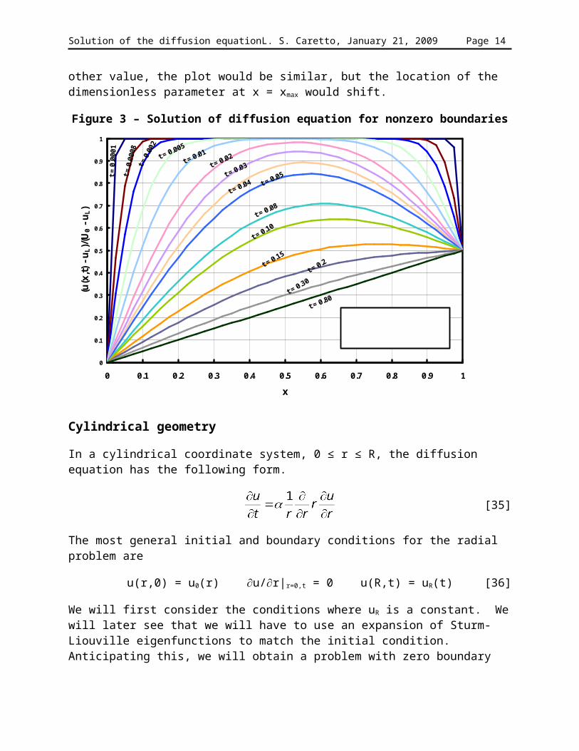
In this equation the dimensionless ratio, [u(x,t) – uL] / (U0 – uL) depends on the dimensionless distance x/xmax, dimensionless time, = αt/(xmax)2, and the ratio of initial and boundary conditions, (uR – uL) / (U0 – uL). A plot of this result for (uR – uL) / (U0 – uL) = 0.5 is shown in Figure 3. This plot shows that the steady-state solution is a linear profile with the expected boundary values for [u(x,t) – uL] / (U0 – uL); these are zero at x = 0 and (uR – uL) / (U0 – uL) = 0.5 at x = xmax. If we changed the value of the parameter (uR – uL) / (U0 – uL) from 0.5 to some other value, the plot would be similar, but the location of the dimensionless parameter at x = xmax would shift.

Figure 3 – Solution of diffusion equation for nonzero boundaries

t = 0

.00 0

1t =

0.0

008

t = 0

.002

t = 0.005

t = 0.01t = 0.02

t = 0.03

t = 0.04 t = 0.05

t = 0.08

t = 0.10

t = 0.15

t = 0.2

t = 0.30

t = 0.80

0

0.1

0.2

0.3

0.4

0.5

0.6

0.7

0.8

0.9

1

0 0.1 0.2 0.3 0.4 0.5 0.6 0.7 0.8 0.9 1

x

(u(x

,t) -

u L)/(

U0 -

uL)

(uR - uL) / (U0 - uL) = 0.5 t = (time)/(xmax)2

Cylindrical geometry

In a cylindrical coordinate system, 0 ≤ r ≤ R, the diffusion equation has the following form.

[35]


The most general initial and boundary conditions for the radial problem are

u(r,0) = u0(r) u/r|r=0,t = 0 u(R,t) = uR(t) [36]

We will first consider the conditions where uR is a constant. We will later see that we will have to use an expansion of Sturm-Liouville eigenfunctions to match the initial condition. Anticipating this, we will obtain a problem with zero boundary conditions by splitting u(r,t) into two parts, as we did in equation [20].

u(r,t) = v(r,t) + uR [37]

The new function, v(r,t) satisfies the differential equation in [35] and has v/r = 0 at r = 0 and v = 0 at r = R. Since uR is a constant, the proposed solution in [37] will satisfy the original differential equation and the boundary conditions from equations [35] and [36]. As before, we seek a solution for v(r,t) using separation of variables. We postulate a solution that is the product of two functions, T(t) a function of time only and P(r) a function of the radial coordinate, r, only. With this assumption, our solution becomes.

v(r,t) = P(r)T(t) [38]

We substitute equation [38] for u in equation [35]. Since P(r) is a function of r only and T(t) is a function of t only, we obtain the following result.

[39]

If we divide the final equation through by the product P(r)T(t), we obtain the following result.

[40]

The left hand side of equation [40] is a function of t only; the right hand side is a function of r only. The only way that this can be correct is if both sides equal a constant. As before, we choose the constant to be equal to2. This gives us two ordinary differential equations to solve.

The first equation becomes has the general solution .

The second differential equation in [40] can be written as . The

general solution to this equation is P(r) = BJ0(r) + CY0(r), where J0 and Y0, are the


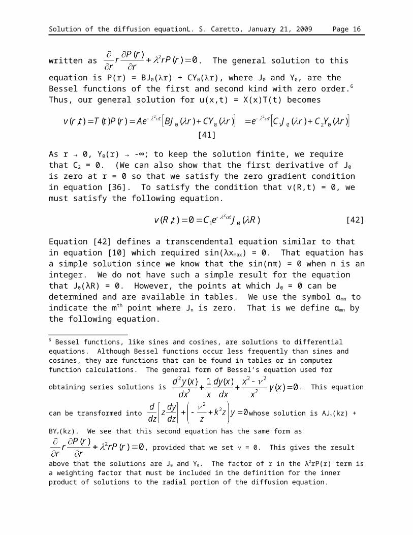
Bessel functions of the first and second kind with zero order.6 Thus, our general solution for u(x,t) = X(x)T(t) becomes

[41]

As r → 0, Y0(r) → -∞; to keep the solution finite, we require that C2 = 0. (We can also show that the first derivative of J0 is zero at r = 0 so that we satisfy the zero gradient condition in equation [36]. To satisfy the condition that v(R,t) = 0, we must satisfy the following equation.

[42]

Equation [42] defines a transcendental equation similar to that in equation [10] which required sin(λxmax) = 0. That equation has a simple solution since we know that the sin(nπ) = 0 when n is an integer. We do not have such a simple result for the equation that J0(λR) = 0. However, the points at which J0 = 0 can be determined and are available in tables. We use the symbol αmn to indicate the mth point where Jn is zero. That is we define αmn by the following equation.

[43]

For example, the first five points at which J0 is zero are for α10 = 2.40483, α20 = 5.52008, α30 = 8.65373, α40 = 11.79153, and α50 = 14.93092. There are an infinite number of such values such that J0(λmr), with λmR = αm0 provides a complete set of orthogonal eigenfunctions that can be used to represent any other function over 0 ≤ r ≤ R. These mn values are called the zeros of Jn.

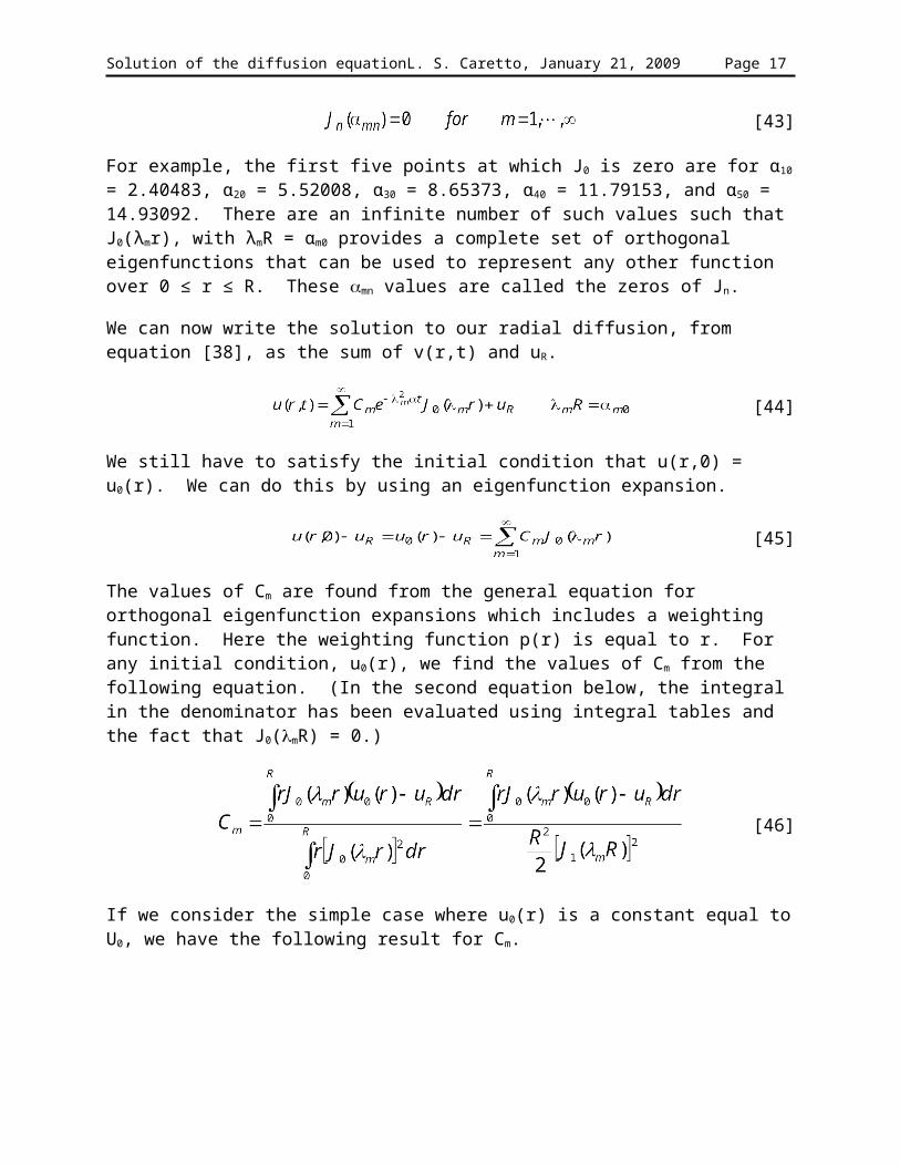
We can now write the solution to our radial diffusion, from equation [38], as the sum of v(r,t) and uR.

[44]

We still have to satisfy the initial condition that u(r,0) = u0(r). We can do this by using an eigenfunction expansion.

6 Bessel functions, like sines and cosines, are solutions to differential equations. Although Bessel functions occur less frequently than sines and cosines, they are functions that can be found in tables or in computer function calculations. The general form of Bessel’s equation used for obtaining series solutions

is . This equation can be transformed into

whose solution is AJ(kz) + BY(kz). We see that this second equation has

the same form as , provided that we set = 0. This gives the result above

that the solutions are J0 and Y0. The factor of r in the λ2rP(r) term is a weighting factor that must be included in the definition for the inner product of solutions to the radial portion of the diffusion equation.


[45]

The values of Cm are found from the general equation for orthogonal eigenfunction expansions which includes a weighting function. Here the weighting function p(r) is equal to r. For any initial condition, u0(r), we find the values of Cm from the following equation. (In the second equation below, the integral in the denominator has been evaluated using integral tables and the fact that J0(mR) = 0.)

[46]

If we consider the simple case where u0(r) is a constant equal to U0, we have the following result for Cm.

[47]

With this result for Cm our solution for u(r,t) with the constant initial condition is written as shown below after some algebra.

[48]

This equation shows the important variables are r/R and αt/R2. We can rearrange this equation to get a dimensionless form, plotted in Figure 4.

[49]


Figure 4 – Solutions to radial diffusion with constant initial condition

tau = 0.0001

tau = 0.0004

tau = 0.002

tau = 0.006

tau = 0.01tau = 0.02tau = 0.04

tau = 0.06tau = 0.08

tau = 0.1

tau = 0.2

tau = 0.3

tau = 0.4

tau = 0.5tau = 0.6

tau = 0.8

tau = 0.15

0.0

0.1

0.2

0.3

0.4

0.5

0.6

0.7

0.8

0.9

1.0

0 0.1 0.2 0.3 0.4 0.5 0.6 0.7 0.8 0.9 1

r/R

[u(r

,t) -

u R] /

(U0

- uR

)

In Figure 4, the notation “tau” denotes the dimensionless time αt/R2. The results in Figure 4 are similar to those in Figure 1 for the rectangular geometry. Here the plot from 0 to R covers half the cylinder and is equivalent to the plot in Figure 1 that covered only half of the one-dimensional region.

Mixed boundary condition

Boundary conditions on differential equations can be expressed in terms of the value of u at the boundary, the gradient of u at the boundary, or a combination of the two. The boundary condition which is an equation relating the value of u and its gradient at the boundary is called a mixed boundary condition.

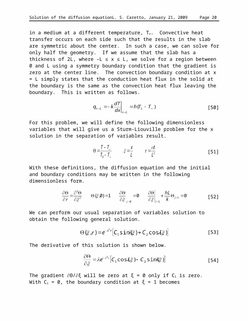
In this example we consider a problem of one dimensional heat conduction. Here we will explicitly use the temperature, T, as the dependent variable (instead of u) and note that α in this case is called the thermal diffusivity. We consider the case where a slab, initially at a constant temperature, T0, is placed in a medium at a different temperature, T∞. Convective heat transfer occurs on each side such that the results in the slab are symmetric about the center. In such a case, we can solve for only half the geometry. If we assume that the slab has a thickness of 2L, where –L ≤ x ≤ L, we solve for a region between 0 and L using a symmetry boundary condition that the gradient is zero at the center line. The convection boundary condition at x = L simply states that the conduction heat flux in the solid at the boundary is the same as the convection heat flux leaving the boundary. This is written as follows.


[50]

For this problem, we will define the following dimensionless variables that will give us a Sturm-Liouville problem for the x solution in the separation of variables result.

[51]

With these definitions, the diffusion equation and the initial and boundary conditions may be written in the following dimensionless form.

[52]

We can perform our usual separation of variables solution to obtain the following general solution.

[53]

The derivative of this solution is shown below.

[54]

The gradient Θ/ξ will be zero at ξ = 0 only if C1 is zero. With C1 = 0, the boundary condition at ξ = 1 becomes

[55]

We can rearrange this equation to obtain a transcendental equation for λ.

[56]

The roots of this equation can be visualized as the points were the plot of a straight line through the origin with a slope of k/hL intersects with the plot of the cotangent. Such a plot is shown in Figure 5 for hL/k = 1.


Figure 5 – Eigenvalues for convection problem

-25

-20

-15

-10

-5

0

5

10

15

20

25

0 2 4 6 8 10 12 14 16 18 20

x

Func

tions Line

CotangentIntersections

In this problem, the eigenfunctions are cos(λmx), but the values of λm do not have a simple equation such as they did in previous problems with simpler boundary conditions. Instead the values of λm for this problem, similar to those for the eigenvalues for J0, are not evenly spaced and have to be found by numerical solutions. The first few values of λm for hL/k = 1 are7 λ1 = 0.860333589, λ2 = 3.425618459, λ3 = 6.437298179, λ4 = 9.529334405, λ5 = 12.64528722, λ6 = 15.77128487, and λ7 = 18.90240996. Changing the value of hL/k would change the slope of the line in Figure 5 and consequently change the intersection points. As m increases, the values of λm increase and the intersections come closer to an integer value of π where the cotangent goes to infinity. For example, λ7 = 18.90240996 is close to 6 π = 18.85.

Even though the eigenvalues, λm, are not evenly spaced, the part of the separation-of-variables problem that was solved for the ξ dependence is a Sturm-Liouville problem, so we know that we can expand any function, representing the initial condition, in terms of these eigenfunctions.

As usual, the most general solution for Θ is a sum of all the eigenfunctions that satisfy the differential equations and the boundary conditions.

[57]

7 You can observe that these values of l are the intersections indicated by the red dots in Figure 5.


If, for the moment, we regard T0 as some arbitrary measure of a variable initial temperature profile, we can use an eigenfunction expansion to fit any initial condition, Θ(ξ,0) = Θ0(ξ) = (T0(L) – T)/(T0 - T∞).

[58]

We have the usual equation for the eigenfunction expansion, where we can find the integral in the denominator from integral tables.

[59]

In particular for a constant initial temperature, T0, Θ0 = 1, and Cm is found as follows.

[60]

Substituting this expression for Cm into equation [57] gives our solution for the dimensionless temperature, Θ, assuming a constant initial temperature.

[61]

The solution is plotted for hL/k = 1 in Figure 6 and for hL/k = 10 in Figure 7.Both solutions are different from the earlier ones in which the boundary temperature was set to a new value at zero time. Here, the boundary temperature decreases over time because of convection heat transfer with the environment. With hL/k = 10, the convection is ten times as strong as it is with hL/k = 1. This leads to a more rapid change in temperature and a greater temperature gradient (i.e., greater heat transfer) at the x = L boundary.

Gradient boundary condition

Consider the diffusion equation with zero gradient boundary conditions shown below.

[62]


Figure 6. Convection Boundary Condition, hL/k = 1

tau = 0.02tau = 0.05tau = 0.1tau = 0.2

tau = 0.5

tau = 1

tau = 2

tau = 3

tau = 4

tau = 0.75

tau = 1.5

0

0.1

0.2

0.3

0.4

0.5

0.6

0.7

0.8

0.9

1

0 0.1 0.2 0.3 0.4 0.5 0.6 0.7 0.8 0.9 1

x/L

Dim

ensi

onle

ss T

empe

ratu

re

Figure 7. Convection Boundary Condition, hL/k = 10

tau = 0.003

tau = 0.005

tau = 0.01

tau = 0.02tau = 0.05tau = 0.2

tau = 0.75

tau = 1

tau = 1.5

tau = 0.1

tau = 0.5

tau = 0.35

0

0.1

0.2

0.3

0.4

0.5

0.6

0.7

0.8

0.9

1

0 0.1 0.2 0.3 0.4 0.5 0.6 0.7 0.8 0.9 1

x/L

Dim

ensi

onle

ss T

empe

ratu

re

The same process that was used to solve equation [1] can be applied to equation [62] to obtain the following solution.


[63]

The constants in equation [63] are given by the following equation.

[64]

As t → , the exponential terms will vanish and the only term that will be left in the

solution is the C0 term. This gives the result that .

Physically, this result tells us what happens when there is no flux into the region. (Recall that the flux of physical quantities described by the diffusion equation is proportional to the gradient; thus a zero gradient means no flux.) With no flux added to the region, the final potential at all points in the region is simply the average of the initial condition.

Nonzero gradients on two sides of a one-dimensional geometry

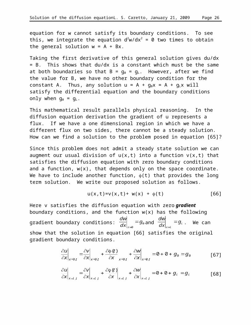
This section should be omitted at first reading. Go directly to the heading “Mixed boundary condition in a cylinder” on page 25. If we want to consider two nonzero gradients we have a problem that does not have a steady-state solution unless both gradients are the same. Even if both gradients are the same the usual notion of a solution in terms of two variables, u(x,t) = v(x,t) + w(x) will not have a unique solution. To see this, consider the following problem.

[65]

A solution of the form u(x,t) = v(x,t) + w(x) where v(x,t) satisfies the diffusion equation with zero gradient boundary conditions and w(x) satisfies the equation d2w/dx2 = 0 with the boundary conditions that dw/dx = g0 at x = 0 and dw/dx = gL at x = L will satisfy the differential equation. However, the equation for w cannot satisfy its boundary conditions. To see this, we integrate the equation d2w/dx2 = 0 two times to obtain the general solution w = A + Bx.

Taking the first derivative of this general solution gives du/dx = B. This shows that du/dx is a constant which must be the same at both boundaries so that B = g0 = gL. However, after we find the value for B, we have no other boundary condition for the constant A. Thus, any solution u = A + g0x = A + gLx will satisfy the differential equation and the boundary conditions only when g0 = gL.

This mathematical result parallels physical reasoning. In the diffusion equation derivation the gradient of u represents a flux. If we have a one dimensional region in


which we have a different flux on two sides, there cannot be a steady solution. How can we find a solution to the problem posed in equation [65]?

Since this problem does not admit a steady state solution we can augment our usual division of u(x,t) into a function v(x,t) that satisfies the diffusion equation with zero boundary conditions and a function, w(x), that depends only on the space coordinate. We have to include another function, (t) that provides the long term solution. We write our proposed solution as follows.

u(x,t)=v(x,t)+ w(x) + (t) [66]

Here v satisfies the diffusion equation with zero gradient boundary conditions, and the

function w(x) has the following gradient boundary conditions: and

. We can show that the solution in equation [66] satisfies the original gradient boundary conditions.

[67]

[68]

The initial condition for v can de derived from the initial condition for u:

[69

If we substitute equation [66] into the diffusion equation and note that w(x) is a function of x only and (t) is a function of time only, we obtain the following result.

[70]

Since v satisfies the diffusion equation, the v terms in the last expression cancel leaving the following relationship between and w.

[71]

We see that equation [71] has a function of t on one side and a function of x on the other side. Just as in the solution of an original partial differential equation by separation of variables, the only way that a function of time can equal a function of x is if both functions equal a constant. Thus, we can rewrite this equation in the same way as we usually apply separation of variables.

[72]


This gives two ordinary differential equations whose solutions are known.

[73]

We can apply the boundary conditions on w to evaluate A and C.

[74]

With the constants just found we can write the solutions for (t) and w(x) as follows.

[75]

The solution for v(x,t) is the solution to the diffusion equation with zero gradient boundary conditions. This solution is an infinite series in the cosine of nx/L, which was given in equation [63].

[76]

The solution for u(x,t) = v(x,t) + w(x) + (t) is then found by combining equations [73] and [76].

[77]

Before substituting the results of equation [74] for A and C, we will consider the initial condition on v: v(x,0) = f(x) – (0) – w(x) = f(x) – B – (A/)(x2/2) – Cx – D. Satisfying this initial condition requires

[78]

We can determine the coefficients Cn by an eigenfunction expansion. We use a separate integration for the n = 0 eigenfunction, cos(0) = 1, because it has a different normalization constant.


[79]

We thus find the following result for C0

[80]

To get the remaining values of Cn, we multiply both sides of the initial condition equation by cos(mx/L) and integrate from 0 to L. Applying the orthogonality relationship for the cosine eigenfunctions gives the following result for m > 0.

[81]

The integral for the terms B and D vanishes as shown below.

[82]

Combining equations [81] and [82] gives the following expression for Cm when m ≥ 1.

[83]

If we substitute equations [80] and [83] into equation [77] we obtain the following equation for u(x,t).

[84]


The B and D terms in this equation cancel so these terms do not enter the solution.8 The following steps can be used to modify equation [84]: (1) use the equations in [74] to

replace A and C; (2) use the definition of the average initial condition, ,

to replace the integral in equation [84]; and (3) use the symbol, Cm, in place of the full expression used in [84]. With these steps the following result obtains after some algebra.

[85]

If we consider a problem with such a large value of t that the terms in the summation are negligible, we can integrate equation [85] to find the (spatial) average value of u(x,t) at any time. In this integration there is a large amount of cancellation leading to the result shown below.

[86]

In this case of large , the average value of u is increasing or decreasing with time depending on the sign of gL – g0.

For large times, the exponential term in the summation of equation [85] will vanish; removing this summation from equation [85] gives the large time limit for the solution shown in equation [87].

[87]

At this point the change in u with time is . This derivative is not a function

of x or t.9 At any value of x then, the change in u(x,t) at any x location, u(x,t2) – u(x,t1),

8 In many approaches to this problem the functions and w are defined so that (0) = w(0) = 0. This drops the constants B and D early in the derivation. However, there is no physical reason for setting these conditions; they are only a convenience to rewrite the derivation in a simpler manner once we know the solution.9 A comparison of equations [86] and [87] shows that two related quantities have the same value:

The derivative on the left is the average (over x) at any time; the derivative on the right is the value at any x for large times. The two equations are consistent. At large times, the derivative at any x has a constant value. Thus the average (over x) will have the same value. Equation [86] tells us that the average (over x) will have this same value at any (large) time.


will be the same for any given time difference, t2 – t1.

[88]

At large times then, the spatial profile of u(x,t) will not change with x. At any value of x the change in u from one time point to another will be the same. This change in u will be an increase if gL > g0; it will be a decrease if gL < g0, and there will be no change in u if gL = g0. In the case where g0 = gL, equation [87] gives

[89]

In this case where the flux is the same constant at both boundaries, the long-time potential is the average of the initial condition plus a linear gradient whose slope is the constant flux term, g0 = gL.

Mixed boundary condition in a cylinder

The problem of diffusion in a cylindrical coordinate system, 0 ≤ r ≤ R, for a fixed boundary condition at the outer radius was treated above, starting with equations [35] and [36]. If there is a mixed boundary condition at the outer radius of the cylinder, the initial and boundary conditions for this problem become.

u(r,0) = u0(r) u/r|r=0,t = 0 –ku/r|r=R,t = h(u – u) [90]

In order to solve this problem, we will first define a new variable, v(r,t) as we did in equation [37], to give a zero boundary condition at r = R.

v(r,t) = u(r,t) – u [91]

With this definition, the boundary condition at r = R becomes

–kv/r|r=R,t = hv(R,t) or (k/h)v/r|r=R,t + v(R,t) = 0 [92]

The solution of the differential equation [35] proceeds in the same manner as done previously, leading to the following equation, similar to equation [42].

[93]

We apply this solution to the boundary condition at r = R, using the result that dJ0(x)/dx = –J1(x) to give the following result.

[94]


Dividing by the constant, C, and the exponential term and defining = R gives the following results.

[95]

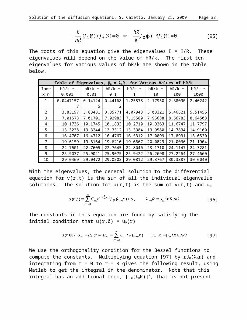
The roots of this equation give the eigenvalues = /R. These eigenvalues will depend on the value of hR/k. The first ten eigenvalues for various values of hR/k are shown in the table below.

Table of Eigenvalues, n = nR, for Various Values of hR/kIndex

,nhR/k = 0.001

hR/k = 0.01

hR/k = 0.1

hR/k = 1

hR/k = 10

hR/k = 100

hR/k = 1000

1 0.04471577 0.141245 0.441682 1.25578 2.17950 2.38090 2.402422 3.83197 3.83431 3.85771 4.07948 5.03321 5.46521 5.514563 7.01573 7.01701 7.02983 7.15580 7.95688 8.56783 8.645084 10.1736 10.1745 10.1833 10.2710 10.9363 11.6747 11.77975 13.3238 13.3244 13.3312 13.3984 13.9580 14.7834 14.91606 16.4707 16.4712 16.4767 16.5312 17.0099 17.8931 18.05307 19.6159 19.6164 19.6210 19.6667 20.0829 21.0036 21.19048 22.7601 22.7605 22.7645 22.8040 23.1710 24.1147 24.32819 25.9037 25.9041 25.9075 25.9422 26.2698 27.2264 27.4660

10 29.0469 29.0472 29.0503 29.0812 29.3767 30.3387 30.6040

With the eigenvalues, the general solution to the differential equation for v(r,t) is the sum of all the individual eigenvalue solutions. The solution for u(r,t) is the sum of v(r,t) and u.

[96]

The constants in this equation are found by satisfying the initial condition that u(r,0) = u0(r).

[97]

We use the orthogonality condition for the Bessel functions to compute the constants. Multiplying equation [97] by rJ0(nr) and integrating from r = 0 to r = R gives the following result, using Matlab to get the integral in the denominator. Note that this integral has an additional term, [J0(mR)]2, that is not present in equation [46]. In that equation, the eigenvalue equation, J0(mR) = 0, sets this term to zero.

[98]


As before, we consider the simplest case where u0(r) is a constant equal to U0; this gives the following result for Cm.

[99]

Substituting this result for Cm into equation [96] for u(r,t) gives the solution for the constant initial condition shown below after some algebra.

[100]

This equation can be rearranged into the following form.

[101]

Equation [101] shows the explicit dependence of a dimensionless potential difference

on a dimensionless radial distance, r/R, and a dimensionless time, t/R2. In

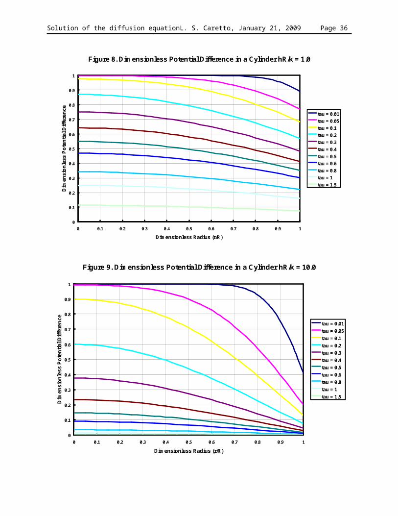
addition, this solution depends on the ratio hR/k since the eigenvalues, m depend on this parameter. The results of calculations for hR/k = 1 and hR/k = 10 are shown in the Figures 8 and 9 as plots of dimensionless potential versus dimensionless radius with dimensionless time, tau = t/R2 as a parameter. The comparison between these two figures is similar to the comparison between Figures 6 and 7. Comparing Figures 6 and 7 showed that a higher values of the parameter hL/k give higher gradients at x = L and shorter times for the values of u at any x location to get closer to u. In Figure 9, with a higher value of hR/k than Figure 8, the gradients at r = R are steeper than in Figure 8 and the times required to reach a given dimensionless u value are shorter.

Spherical geometry

In a spherical coordinate system, 0 ≤ r ≤ the one-dimensional diffusion equation (no angular dependence) has the following form.

[102]


The most general initial and boundary conditions for the radial problem are

u(r,0) = u0(r) u/r|r=0,t = 0 u(R,t) = uR(t) [103]

We will first consider the conditions where uR is a constant. We will later see that we will have to use an expansion of Sturm-Liouville eigenfunctions to match the initial condition. Anticipating this, we will obtain a problem with zero boundary conditions by splitting u(r,t) into two parts, as we did in equation [37] for cylindrical geometry.

u(r,t) = v(r,t) + uR [104]

Figure 8. Dimensionless Potential Difference in a Cylinder hR/k = 1.0

0

0.1

0.2

0.3

0.4

0.5

0.6

0.7

0.8

0.9

1

0 0.1 0.2 0.3 0.4 0.5 0.6 0.7 0.8 0.9 1

Dimensionless Radius (r/R)

Dim

ensi

onle

ss P

oten

tial D

iffer

ence

tau = 0.01tau = 0.05tau = 0.1tau = 0.2tau = 0.3tau = 0.4tau = 0.5tau = 0.6tau = 0.8tau = 1tau = 1.5


Figure 9. Dimensionless Potential Difference in a Cylinder hR/k = 10.0

0

0.1

0.2

0.3

0.4

0.5

0.6

0.7

0.8

0.9

1

0 0.1 0.2 0.3 0.4 0.5 0.6 0.7 0.8 0.9 1

Dimensionless Radius (r/R)

Dim

ensi

onle

ss P

oten

tial D

iffer

ence

tau = 0.01tau = 0.05tau = 0.1tau = 0.2tau = 0.3tau = 0.4tau = 0.5tau = 0.6tau = 0.8tau = 1tau = 1.5

The new function, v(r,t) satisfies the differential equation in [102] and has v/r = 0 at r = 0 and v = 0 at r = R. Since uR is a constant, the proposed solution in [104] will satisfy the original differential equation and the boundary conditions from equations [102] and [103]. As before, we seek a solution for v(r,t) using separation of variables. We postulate a solution that is the product of two functions, T(t) a function of time only and P(r) a function of the radial coordinate, r, only. With this assumption, our solution becomes.

v(r,t) = P(r)T(t) [105]

We substitute equation [105] for u in equation [102]. Since P(r) is a function of r only and T(t) is a function of t only, we obtain the following result.

[106]

If we divide the final equation through by the product P(r)T(t), we obtain the following result.


[107]

The left hand side of equation [107] is a function of t only; the right hand side is a function of r only. The only way that this can be correct is if both sides equal a constant. As before, we choose the constant to be equal to2. This gives us two ordinary differential equations to solve.

The first equation becomes has the general solution .

The second ordinary differential equation in [107] can be written as follows.

. [108]

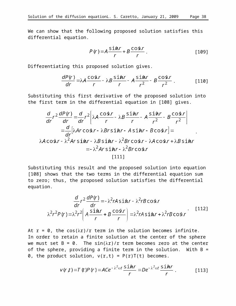
We can show that the following proposed solution satisfies this differential equation.

. [109]

Differentiating this proposed solution gives.

. [110]

Substituting this first derivative of the proposed solution into the first term in the differential equation in [108] gives.

. [111]

Substituting this result and the proposed solution into equation [108] shows that the two terms in the differential equation sum to zero; thus, the proposed solution satisfies the differential equation.

. [112]

At r = 0, the cos(r)/r term in the solution becomes infinite. In order to retain a finite solution at the center of the sphere we must set B = 0. The sin(r)/r term becomes zero


at the center of the sphere, providing a finite term in the solution. With B = 0, the product solution, v(r,t) = P(r)T(t) becomes.

. [113]

We now have to satisfy the condition that v(r,t) = 0 at r = R,

. [114]

This gives the expected eigenvalue solution that R must be an integral multiple of .

[115]

The general solution for v(r,t) is a sum of all eigenvalue solutions, each multiplied by a different constant, Dn. From equation [104], we know that the solution we want for u(r,t) = v(r,t) + uR. Thus, our general solution for u(r,t) is written as follows

[116]

We still have to satisfy the initial condition that u(r,0) = u0(r). Substituting this condition for t = 0 into equation [116] gives

[117]

As usual, the eigenfunctions (1/r)sin(nr/R) form a complete set of orthogonal eigenfunctions in the interval 0 ≤ r ≤ R; however, the Sturm-Liouville problem defined in equation [108] has a weighting factor of r2 that must be used in the orthogonality integral. If we multiply both sides of equation [117] by r2(1/r)sin(mr/R)dr, where m is another integer, and integrate from zero to R, we get the following result. The steps used here are similar to those in equation [14].

[118]

Solving for Dm and evaluating the final integral gives the following result, which is similar to equation [15].


[119]

As an example, consider the simplest case where u0(r) = U0, a constant. In this case we find Dm as follows.

[120]

Since cos(m) is 1 when m is even and –1 when m is odd, we can write the final result for Dm as shown below.

[121]

Substituting this result into equation [116] gives the following solution to the diffusion equation when u0(x) = U0, a constant, and the boundary temperatures are zero.

[122]

We can rearrange this equation to introduce nr in the summation and create the following dimensionless form.

[123]

The dimensionless ratio on the left of this equation depends on the dimensionless radius r/R and the dimensionless time, expressed as a Fourier number, t/R2.

Spherical geometry with mixed boundary condition


We still have the differential equation in [102], but we now have the following boundary conditions:

u(r,0) = u0(r) u/r|r=0,t = 0 –ku/r|r=R,t = h(ur=R – u) [124]

In order to solve this problem, we will first define a new variable, v(r,t) as we did in equation [91], for the mixed boundary condition for the cylinder, to give a zero boundary condition at r = R.

v(r,t) = u(r,t) – u [125]

The boundary conditions for this new variable, v(r,t) are shown below.

v(r,0) = u0(r) – u v/r|r=0,t = 0 –kv/r|r=R,t = hvr=R [126]

The general solution for v(r,t) is will be the same as the solution to the problem with fixed temperature given in equation [113]. This equation is copied below.

. [113]

In order to satisfy the boundary condition at r = R, –kv/r|r=R,t = hvr=R, with equation [113], we have to satisfy the following equation.

. [127]

Dividing the final equation by (De-2tk/R2)sin R gives.

[128]

The roots of this equation are the eigenvalues of the solution to the present problem. These eigenvalues will depend on the dimensionless group hR/k. We can compare this equation with equation [56], which gives the eigenvalues for the rectangular slab with a convection boundary condition. The roots of equation [56] are the values of that satisfy = hL/k cot(). If we define = R in equation [128], the roots of that equation are the values of that satisfy = (1 – hR/k) tan(). For hR/k = 1, this equation can be written as cot() = 0. Thus, the eigenvalues for hR/k = 1 are simply the zeros of the cotangent, (2n – 1)/2, where n is an integer greater than or equal to one.10 For other values of hR/k, we can write the eigenvalue equation as /(1 – hR/k) = tan(). For hR/k < 1, the roots of the equation [128] will be the intersection of the tangent curve with a line, starting at zero and having a positive slope. This will yield eigenvalues as shown in Figure 10. The straight line for values of hR/k greater than one will have a negative slope as shown in Figure 11.

10 Note that = 0 is not a root of cot() = 0. As → 0, cot() → 1.


Regardless of the behavior of the eigenvalues, the resulting solution will still have the same form as equation [116]; however, this solution has u in place of uR, and the eigenvalues are different.

[129]

We still have to satisfy the initial condition that u(r,0) = u0(r). Substituting this condition for t = 0 into equation [129] gives

[130]

As in equation [117], the eigenfunctions (1/r)sin(nr) form a complete set of orthogonal eigenfunctions in the interval 0 ≤ r ≤ R, with a weighting factor of r2 that must be used in the orthogonality integral.


Figure 10. Sphere Convection Eigenvalues for hR/k = 0.1

-20

-15

-10

-5

0

5

10

15

20

0 2 4 6 8 10 12 14 16 18 20

Func

tions Line

TangentIntersections


Figure 11. Sphere Convection Eigenvalues for hR/k = 2.0

-20

-15

-10

-5

0

5

10

15

20

0 2 4 6 8 10 12 14 16 18 20

Func

tions Line

TangentIntersections

Repeating the process used in obtaining equation [118] – multiplying both sides of equation [130] by r2(1/r)sin(mr)dr, where m is another eigenvalue, and integrating from zero to R – gives the following result.

[131]

Solving for Dm and evaluating the final integral gives the following result, which is similar to equation [119].

[132]

The integral of sin2(mr) was found by symbolic integration using Matlab. This integral has an additional term that was not present in equation [119], where mR = m which gives sin(mR) = 0.


As usual we will apply this equation to the simplest case where u0(r) = U0, a constant. In this case we find the numerator in the integral for Dm as follows.

[133]

Solving for Dm and performing some algebraic rearrangement gives the final result for Dm.

[134]

Substituting this expression for Dm into equation [129] gives the following solution for u(r,t) in this case.

[135]

We can obtain a dimensionless form by introducing m = nR and performing some algebraic rearrangement.

[136]

This equation shows that the dimensionless ratio, , depends explicitly on the

dimensionless radius, r/R and the dimensionless time (Fourier number) t/R2. In addition, there is an implicit dependence on the dimensionless group hR/k, known as the Biot number, through the eigenvalue n. A plot of equation [136] for hR/k = 1 is shown in Figure 12.


Figure 12. Dimensionless Potential Difference in a Sphere with hR/k = 1.0

0

0.1

0.2

0.3

0.4

0.5

0.6

0.7

0.8

0.9

1

0 0.1 0.2 0.3 0.4 0.5 0.6 0.7 0.8 0.9 1

Dimensionless time, t/R2

tau = 0.01tau = 0.1tau = 0.2tau = 0.3tau = 0.4tau = 0.5tau = 0.6tau = 0.8tau = 1tau = 2tau = 3tau = 4tau = 5

solution of the diffusion equation - california state …lcaretto/me501b/diffusion.doc · web...

Documents