solution techniques for elementary partial differential ... · for elementary partial differential...
TRANSCRIPT


Second Edition
Solution Techniques for Elementary Partial Differential Equations
K10569_FM.indd 1 4/28/10 9:50:09 AM

Second Edition
Solution Techniques for Elementary Partial Differential Equations
Christian ConstandaUniversity of Tulsa
Oklahoma
K10569_FM.indd 2 4/28/10 9:50:09 AM

Second Edition
Solution Techniques for Elementary Partial Differential Equations
Christian ConstandaUniversity of Tulsa
Oklahoma
K10569_FM.indd 3 4/28/10 9:50:09 AM

Chapman & Hall/CRCTaylor & Francis Group6000 Broken Sound Parkway NW, Suite 300Boca Raton, FL 33487-2742
© 2010 by Taylor and Francis Group, LLCChapman & Hall/CRC is an imprint of Taylor & Francis Group, an Informa business
No claim to original U.S. Government works
Printed in the United States of America on acid-free paper10 9 8 7 6 5 4 3 2 1
International Standard Book Number-13: 978-1-4398-1140-5 (Ebook-PDF)
This book contains information obtained from authentic and highly regarded sources. Reasonable efforts have been made to publish reliable data and information, but the author and publisher cannot assume responsibility for the validity of all materials or the consequences of their use. The authors and publishers have attempted to trace the copyright holders of all material reproduced in this publication and apologize to copyright holders if permission to publish in this form has not been obtained. If any copyright material has not been acknowledged please write and let us know so we may rectify in any future reprint.
Except as permitted under U.S. Copyright Law, no part of this book may be reprinted, reproduced, transmit-ted, or utilized in any form by any electronic, mechanical, or other means, now known or hereafter invented, including photocopying, microfilming, and recording, or in any information storage or retrieval system, without written permission from the publishers.
For permission to photocopy or use material electronically from this work, please access www.copyright.com (http://www.copyright.com/) or contact the Copyright Clearance Center, Inc. (CCC), 222 Rosewood Drive, Danvers, MA 01923, 978-750-8400. CCC is a not-for-profit organization that provides licenses and registration for a variety of users. For organizations that have been granted a photocopy license by the CCC, a separate system of payment has been arranged.
Trademark Notice: Product or corporate names may be trademarks or registered trademarks, and are used only for identification and explanation without intent to infringe.
Visit the Taylor & Francis Web site athttp://www.taylorandfrancis.com
and the CRC Press Web site athttp://www.crcpress.com

For Lia


Contents
Foreword xi
Preface to the Second Edition xiii
Preface to the First Edition xv
Chapter 1. Ordinary Differential Equations: Brief Review 1
1.1. First-Order Equations 11.2. Homogeneous Linear Equations with Constant Coefficients 31.3. Nonhomogeneous Linear Equations with Constant Coefficients 51.4. Cauchy–Euler Equations 61.5. Functions and Operators 7
Exercises 9
Chapter 2. Fourier Series 11
2.1. The Full Fourier Series 112.2. Fourier Sine Series 172.3. Fourier Cosine Series 212.4. Convergence and Differentiation 23
Exercises 24
Chapter 3. Sturm–Liouville Problems 27
3.1. Regular Sturm–Liouville Problems 273.2. Other Problems 393.3. Bessel Functions 413.4. Legendre Polynomials 473.5. Spherical Harmonics 50
Exercises 54
Chapter 4. Some Fundamental Equations of MathematicalPhysics 59
4.1. The Heat Equation 594.2. The Laplace Equation 674.3. The Wave Equation 734.4. Other Equations 78
Exercises 81

viii
Chapter 5. The Method of Separation of Variables 83
5.1. The Heat Equation 835.2. The Wave Equation 955.3. The Laplace Equation 1015.4. Other Equations 1095.5. Equations with More than Two Variables 113
Exercises 124
Chapter 6. Linear Nonhomogeneous Problems 131
6.1. Equilibrium Solutions 1316.2. Nonhomogeneous Problems 136
Exercises 140
Chapter 7. The Method of Eigenfunction Expansion 143
7.1. The Heat Equation 1437.2. The Wave Equation 1497.3. The Laplace Equation 1527.4. Other Equations 155
Exercises 159
Chapter 8. The Fourier Transformations 165
8.1. The Full Fourier Transformation 1658.2. The Fourier Sine and Cosine Transformations 1728.3. Other Applications 179
Exercises 181
Chapter 9. The Laplace Transformation 187
9.1. Definition and Properties 1879.2. Applications 192
Exercises 202
Chapter 10. The Method of Green’s Functions 205
10.1. The Heat Equation 20510.2. The Laplace Equation 21310.3. The Wave Equation 217
Exercises 223

ix
Chapter 11. General Second-Order Linear Partial
Differential Equations with Two IndependentVariables 227
11.1. The Canonical Form 22711.2. Hyperbolic Equations 23111.3. Parabolic Equations 23511.4. Elliptic Equations 238
Exercises 239
Chapter 12. The Method of Characteristics 241
12.1. First-Order Linear Equations 24112.2. First-Order Quasilinear Equations 24812.3. The One-Dimensional Wave Equation 24912.4. Other Hyperbolic Equations 256
Exercises 260
Chapter 13. Perturbation and Asymptotic Methods 263
13.1. Asymptotic Series 26313.2. Regular Perturbation Problems 26613.3. Singular Perturbation Problems 274
Exercises 280
Chapter 14. Complex Variable Methods 285
14.1. Elliptic Equations 28514.2. Systems of Equations 291
Exercises 294
Answers to Odd-Numbered Exercises 297
Appendix 313
Bibliography 319
Index 321


Foreword
It is often difficult to persuade undergraduate students of the importance ofmathematics. Engineering students in particular, geared towards the prac-tical side of learning, often have little time for theoretical arguments andabstract thinking. In fact, mathematics is the language of engineering andapplied science. It is the vehicle by which ideas are analyzed, developed, andcommunicated. It is no accident, therefore, that any undergraduate engi-neering curriculum requires several mathematics courses, each one designedto provide the necessary analytic tools to deal with questions raised by en-gineering problems of increasing complexity, for example, in the modelingof physical processes and phenomena. The most effective way to teach stu-dents how to use these mathematical tools is by example. The more workedexamples and practice exercises a textbook contains, the more effective itwill be in the classroom.
Such is the case with Solution Techniques for Elementary Partial Differ-ential Equations by Christian Constanda. The author, a skilled classroomperformer with considerable experience, understands exactly what studentswant and has given them just that: a textbook that explains the essenceof the method briefly and then proceeds to show it in action. The bookcontains a wealth of worked examples and exercises (half of them with an-swers). An Instructor’s Manual with solutions to each problem and a .pdffile for use on a computer-linked projector are also available. In my opin-ion, this is quite simply the best book of its kind that I have seen thusfar. The book not only contains solution methods for some very importantclasses of PDEs, in easy-to-read format, but is also student-friendly andteacher-friendly at the same time. It is definitely a textbook that should beadopted.
Professor Peter SchiavoneDepartment of Mechanical EngineeringUniversity of AlbertaEdmonton, AB, Canada


Preface to the Second Edition
In direct response to constructive suggestions received from some of theusers of the book, this second edition contains a number of enhancements.
• Section 1.4 (Cauchy–Euler Equations) has been added to Chapter 1.
• Chapter 3 includes three new sections: 3.3 (Bessel Functions), 3.4(Legendre Polynomials), and 3.5 (Spherical Harmonics).
• The new Section 4.4 in Chapter 4 lists additional mathematical modelsbased on partial differential equations.
• Sections 5.4 and 7.4 have been added to Chapters 5 and 7, respectively,to show—by means of examples—how the methods of separation ofvariables and eigenfunction expansion work for equations other thanheat, wave, and Laplace.
• Supplementary applications of the Fourier transformations are nowshown in Section 8.3.
• The method of characteristics is applied to more general hyperbolicequations in the additional Section 12.4.
• Chapter 14 (Complex Variable Methods) is entirely new.
• The number of worked examples has increased from 110 to 143, andthat of the exercises has almost quadrupled—from 165 to 604.
• The tables of Fourier and Laplace transforms in the Appendix havebeen considerably augmented.
• The first coefficient of the Fourier series is now 12 a0 instead of the pre-
vious a0. Similarly, the direct and inverse full Fourier transformationsare now defined with the normalizing factor 1/
√2π in front of the inte-
gral; the Fourier sine and cosine transformations are defined with thefactor
√2/π .
While I still believe that students should be encouraged not to use elec-tronic computing devices in their learning of the fundamentals of partialdifferential equations, I have made a concession when it comes to exam-

xiv PREFACE TO THE SECOND EDITION
ples and exercises involving special functions, transcendental equations, orexceedingly lengthy integration. The (new) exercises that require compu-tational help because they are not solvable by elementary means have beengiven italicized numerical labels. Their answers are worked out with the
Mathematica R software and are given in the form that package produceswith full simplification. I have also included a few extra formulas in tableA1 in the Appendix to assist with the evaluation of some basic integralsthat occur frequently in the solution of the exercises.
The material in this edition seems to exceed what can normally be coveredin a one-semester course, even when taught at a brisk pace. If a moreleisurely pace is adopted, then the material might be stretched to providework for two semesters.
I wish to thank all the readers who sent me their comments and urgethem to continue to do so in the future. It is only with their help that thisbook may undergo further improvement.
I would also like to thank Sunil Nair, Sarah Morris, Karen Simon, andKevin Craig at Taylor & Francis for their professional and expeditious han-dling of this project.
Christian ConstandaThe University of TulsaMarch 2010

Preface to the First Edition
There are many textbooks on partial differential equations on the market.The great majority of them are well written and very rigorous, with fullbackground explanations, detailed proofs, and lots of comments. But theyalso tend to be rather voluminous and daunting for the average student.When I ask my undergraduates what they want from a book, their mostcommon answers are (i) to understand without excessive effort most of whatis being said; (ii) to be given full yet concise explanations of the essence ofthe topics discussed, in simple words; (iii) to have many worked examples,preferably of the type found in test papers, so they could learn the var-ious techniques by seeing them in action and thus improve their chancesof passing examinations; and (iv) to pay as little as possible for it in thebookstore. I do not wish to comment on the validity of these answers, butI am prepared to accept that even in higher education the customer maysometimes be right.
This book is an attempt to meet all the above requirements. It is designedas a no-frills text that explains a number of major methods completely butsuccinctly, in everyday classroom language. It does not indulge in multi-page, multicolored spiels. It includes many practical applications with so-lutions, and exercises with selected answers. It has a reasonable number ofpages and is produced in a format that facilitates digital reproduction, thushelping keep costs down.
Teachers have their own individual notions regarding what makes a bookideal for use in coursework. They say—with good reason—that the perfecttext is the one they themselves sketched in their classroom notes but neverhad the time or inclination to polish up and publish. We each choose ourown material, the order in which the topics are presented, and how long wespend on them. This book is no exception. It is based on my experienceof the subject for many years and the feedback received from my teaching’sbeneficiaries. The “use in combat” of an earlier version seems to indicatethat average students can work from it independently, with some occasionalinstructor guidance, while the high flyers get a basic and rapid grounding inthe fundamentals of the subject before progressing to more advanced texts

xvi PREFACE TO THE FIRST EDITION
(if they are interested in further details and want to get a truly sophisticatedpicture of the field). A list, by no means exhaustive, of such texts can befound in the Bibliography.
This book contains no example or exercise that needs a calculating devicein its solution. Computing machines are now part of everyday life and weall use them routinely and extensively. However, I believe that if you reallywant to learn what mathematical analysis is all about, then you shouldexercise your mind and hand the long way, without any electronic help. (Infact, it seems that quite a few of my students are convinced that computersare better used for surfing the Internet than for solving homework problems.)The only prerequisites for reading this book are a first course in calculusand some basic knowledge of certain types of ordinary differential equations.
The topics are arranged in the order I have found to be the most con-venient. After some essential but elementary ODEs, Fourier series, andSturm–Liouville problems are discussed briefly, the heat, Laplace, and waveequations are introduced in quick succession as mathematical models ofphysical phenomena, and then a number of methods (separation of vari-ables, eigenfunction expansion, Fourier and Laplace transformations, andGreen’s functions) are applied in turn to specific initial/boundary valueproblems for each of these equations. There follows a brief discussion ofthe general second-order linear equation with two independent variables.Finally, the method of characteristics and perturbation (asymptotic expan-sion) methods are presented. A number of useful tables and formulas arelisted in the Appendix.
The style of the text is terse and utilitarian. In my experience, theteacher’s classroom performance does more to generate undergraduate en-thusiasm and excitement for a topic than the cold words in a book, howeverskillfully crafted. Since the aim here is to get the students well drilled inthe main solution techniques and not in the physical interpretation of theresults, the latter hardly gets a mention. The examples and exercises areformal, and in many of them the chosen data may not reflect plausible real-life situations. Due to space pressure, some intermediate steps—particularlythe solutions of simple ODEs—are given without full working. It is assumedthat the readers know how to derive them, or that they can refer withoutdifficulty to the summary provided in Chapter 1. Personally, in class I al-
PREFACE TO THE FIRST EDITION xvii
ways go through the full solution regardless, which appears to meet withthe approval of the audience. Details of a highly mathematical nature, in-cluding formal proofs, are kept to a minimum, and when they are given,an assumption is made that any conditions required by the context (forexample, the smoothness and behavior of functions) are satisfied.
An Instructor’s Manual containing the solutions of all the exercises isavailable. Also, on adoption of the book, a .pdf file of the text can besupplied to instructors for use on classroom projectors.
My own lecturing routine consists of (i) using a projector to present askeleton of the theory, so the students do not need to take notes and canfollow the live explanations, and (ii) doing a selection of examples on theboard with full details, which the students take down by hand. I found thatthis sequence of “talking periods” and “writing periods” helps the audiencemaintain concentration and makes the lecture more enjoyable (if what theend-of-semester evaluations say is true).
Wanting to offer students complete, rigorous, and erudite expositions ishighly laudable, but the market priorities appear to have shifted of late.With the current standards of secondary education manifestly lower than inthe past, students come to us less and less equipped to tackle the learningof mathematics from a fundamental point of view. When this becomesunavoidable, they seem to prefer a concise text that shows them the methodand then, without fuss and niceties of form, goes into as many workedexamples as possible. Whether we like it or not, it seems that we haveentered the era of the digest. It is to this uncomfortable reality that thepresent book seeks to offer a solution.
The last stages of preparation of this book were completed while I wasa Visiting Professor in the Department of Mathematical and ComputerSciences at the University of Tulsa. I wish to thank the authorities ofthis institution and the faculty in the department for providing me withthe atmosphere, conditions, and necessary facilities to finish the work ontime. Particular thanks go to the following: Bill Coberly, the head of thedepartment, who helped me engineer several summer visits and a coupleof successful sabbatical years in Tulsa; Pete Cook, who heard my dailymoans and groans from across the corridor and did not complain about
it; Dale Doty, the resident Mathematica R wizard who drew some of the

xviii PREFACE TO THE FIRST EDITION
figures and showed me how to do the others; and the sui generis companyat the lunch table in the Faculty Club for whom, in time-honored academicfashion, no discussion topic was too trivial or taboo and no explanation tooimplausible.
I also wish to thank Sunil Nair, Helena Redshaw, Andrea Demby, andJasmin Naim from Chapman & Hall/CRC for their help with technicaladvice and flexibility over deadlines.
Finally, I would like to state for the record that this book project wouldnot have come to fruition had I not had the full support of my wife, who,not for the first time, showed a degree of patience and understanding farbeyond the most reasonable expectations.
Christian Constanda

Chapter 1Ordinary DifferentialEquations: Brief Review
In the process of solving partial differential equations (PDEs) we usuallyreduce the problem to the solution of certain classes of ordinary differentialequations (ODEs). Here we mention without proof some basic methods forintegrating simple ODEs of the types encountered later in the text. Werestrict our attention to real solutions of ODEs with real coefficients. Inwhat follows, the set of real numbers is denoted by R.
1.1. First-Order Equations
Variables separable equations. The general form of this type of ODE is
y′ =dy
dx= f(x)g(y).
Taking standard precautions, we can rewrite the equation as
dy
g(y)= f(x)dx
and then integrate each side with respect to its corresponding variable.
1.1. Example. For the equation
y2y′ − 2x = 0
the above procedure leads to∫y2dy = 2
∫xdx,
which yields13 y
3 = x2 + c, c = const,
ory(x) = (3x2 + C)1/3, C = const.

2 ORDINARY DIFFERENTIAL EQUATIONS
Linear equations. Their general (normal) form is
y′ + p(x)y = q(x),
where p and q are given functions. Computing an integrating factor μ(x)by means of the formula
μ(x) = exp{∫
p(x)dx},
we obtain the general solution
y(x) =1
μ(x)
∫μ(x)q(x)dx.
An equivalent formula for the general solution is
y(x) =1
μ(x)
[ x∫a
μ(t)q(t)dt + C
], C = const,
where a is any point in the domain where the ODE is satisfied.
1.2. Example. The normal form of the equation
xy′ + 2y − x2 = 0, x �= 0,
is
y′ +2xy = x.
Herep(x) =
2x, q(x) = x,
so an integrating factor is
μ(x) = exp{
2∫dx
x
}= elnx2
= x2.
Then the general solution of the equation is
y(x) =1x2
∫x3 dx =
14x2 +
C
x2, C = const.

HOMOGENEOUS LINEAR EQUATIONS 3
1.2. Homogeneous Linear Equations withConstant Coefficients
First-order equations. These are equations of the form
y′ + ay = 0, a = const.
Such equations can be solved by means of an integrating factor or separationof variables, or by means of the characteristic equation
s+ a = 0,
whose root s = −a yields the general solution
y(x) = Ce−ax, C = const.
1.3. Example. The characteristic equation for the ODE
y′ − 3y = 0
is
s− 3 = 0;
hence, the general solution of the equation is
y(x) = Ce3x, C = const.
Second-order equations. Their general form is
y′′ + ay′ + by = 0, a, b = const.
If the characteristic equation
s2 + as+ b = 0
has two distinct real roots s1 and s2, then the general solution of the givenODE is
y(x) = C1es1x + C2e
s2x, C1, C2 = const.
If s1 = s2 = s0, then
y(x) = (C1 + C2x)es0x, C1, C2 = const.

4 ORDINARY DIFFERENTIAL EQUATIONS
Finally, if s1 and s2 are complex conjugate—that is, s1 = α+iβ, s2 = α−iβ,where α and β are real numbers—then the general solution is
y(x) = eαx[C1 cos(βx) + C2 sin(βx)], C1, C2 = const.
1.4. Remark. When s1 = −s2 = s0, s0 real, the general solution of theequation can also be written as
y(x) = C1y1(x) + C2y2(x), C1, C2 = const,
where y1(x) and y2(x) are any two of the functions
cosh(s0x), sinh(s0x), cosh(s0(x − c)
), sinh
(s0(x− c)
)and c is any nonzero real number. Normally, c is chosen as the point wherea boundary condition is given.
1.5. Example. The characteristic equation for the ODE
y′′ − 3y′ + 2y = 0is
s2 − 3s+ 2 = 0,
with roots s1 = 1 and s2 = 2, so the general solution of the ODE is
y(x) = C1ex + C2e
2x, C1, C2 = const.
1.6. Example. The general solution of the equation
y′′ − 4y = 0is
y(x) = C1e2x + C2e
−2x, C1, C2 = const,
since the roots of its characteristic equation are s1 = −s2 = 2. Accord-ing to Remark 1.4, we have alternative expressions in terms of hyperbolicfunctions. Thus, if y(0) and y(1) are prescribed, then the general solutionshould be written in the form
y(x) = C1 sinh(2x) + C2 sinh(2(x− 1)
), C1, C2 = const;

NONHOMOGENEOUS LINEAR EQUATIONS 5
if y(0) and y′(3) are prescribed, then the preferred form is
y(x) = C1 sinh(2x) + C2 cosh(2(x− 3)
), C1, C2 = const;
and so on.
1.7. Example. The roots of the characteristic equation for the ODE
y′′ + 4y′ + 4y = 0
are s1 = s2 = −2; therefore, the general solution of the ODE is
y = (C1 + C2x)e−2x, C1, C2 = const.
1.8. Example. The general solution of the equation
y′′ + 4y = 0is
y = C1 cos(2x) + C2 sin(2x), C1, C2 = const,
since the roots of its characteristic equation are s1 = 2i and s2 = −2i.
1.9. Remark. The characteristic equation method can also be applied tofind the general solution of homogeneous linear ODEs of higher order.
1.3. Nonhomogeneous Linear Equations withConstant Coefficients
The first-order equations in this category are of the form
y′ + ay = f, a = const;
the second-order equations can be written as
y′′ + ay′ + by = f, a, b = const.
Here f is a given function. The general solution of such equations is the sumof the complementary function (the general solution of the correspondinghomogeneous equation) and a particular integral (a particular solution ofthe nonhomogeneous equation). The latter is usually guessed from thestructure of the function f or may be found by some other method, such asvariation of parameters.

6 ORDINARY DIFFERENTIAL EQUATIONS
1.10. Example. The complementary function for the ODE
y′ − 3y = e−x
isy
CF= Ce3x, C = const.
Seeking a particular integral of the form yP I
= ae−x, a = const, we findfrom the equation that a = −1/4. Consequently, the general solution of thegiven ODE is
y = Ce3x − 14 e
−x, C = const.
1.11. Example. If the function on the right-hand side in Example 1.10is replaced by e3x, then we cannot find a particular integral of the formae3x, a = const, since this is a solution of the corresponding homogeneousequation. Instead, we try y
P I= axe3x and deduce, by replacing in the
ODE, that a = 1; consequently, the general solution is
y = Ce3x + xe3x = (C + x)e3x, C = const.
1.12. Example. For the equation
y′′ + 4y = 4x2
we seek a particular integral of the form
yPI
= ax2 + bx+ c, a, b, c = const.
Direct substitution into the equation yields a = 1, b = 0, and c = −1/2.Since the complementary function is
yCF
= C1 cos(2x) + C2 sin(2x),
it follows that the general solution of the given ODE is
y = C1 cos(2x) + C2 sin(2x) + x2 − 12 , C1, C2 = const.
1.4. Cauchy–Euler Equations
These are second-order linear equations of the form
x2y′′ + αxy′ + βy = 0, α, β = const,

FUNCTIONS AND OPERATORS 7
where, for simplicity, we assume that x > 0. The solution is sought in theform
y = xr, r = const.
Substituting in the equation, we arrive at
r2 + (α− 1)r + β = 0.
If the roots r1 and r2 of this quadratic equation are real and distinct, whichis the case of interest for us, then the general solution of the given ODE is
y = C1xr1 + C2x
r2 , C1, C2 = const.
1.13. Example. Following the above procedure, we see that the differentialequation
2x2y′′ + 3xy′ − y = 0
yieldsr1 = 1, r2 = − 1
2 ,
so its general solution is
y = C1x+ C2x−1/2, C1, C2 = const.
1.5. Functions and Operators
Throughout this book we refer to a function as either f or f(x), although,strictly speaking, the latter denotes the value of f at x. To avoid compli-cated notation, we also write f(x) = c to designate a function f that takesthe same value c = const at all points x in its domain. When c = 0, wesometimes simplify this further to f = 0.
In the preceding sections we mentioned linear equations. Here we clarifythe meaning of this concept.
1.14. Definition. Let X be a space of functions, and let L be an operatoracting on the functions in X according to some rule. The operator L iscalled linear if
L(c1f1 + c2f2) = c1(Lf1) + c2(Lf2)
for any functions f1, f2 in X and any numbers c1, c2. Otherwise, L is callednonlinear.

8 ORDINARY DIFFERENTIAL EQUATIONS
1.15. Example. The operators of differentiation and definite integrationacting on suitable functions of one independent variable are linear, since
L(c1f1 + c2f2) = (c1f1 + c2f2)′ = c1f′1 + c2f
′2 = c1(Lf1) + c2(Lf2),
L(c1f1 + c2f2) =
b∫a
[c1f1(x) + c2f2(x)
]dx
= c1
b∫a
f1(x)dx + c2
b∫a
f2(x)dx = c1(Lf1) + c2(Lf2).
1.16. Example. Let α, β, and γ be given functions. In view of the pre-ceding example, it is easy to verify that the operator L defined by
Lf = αf ′′ + βf ′ + γf
is linear.
1.17. Example. Let L be the operator defined by
Lf = ff ′.
Since
L(c1f1 + c2f2) = (c1f1 + c2f2)(c1f1 + c2f2)′
= c21f1f′1 + c1c2(f1f ′
2 + f ′1f2) + c22f2f
′2
and
c1(Lf1) + c2(Lf2) = c1f1f′1 + c2f2f
′2
are not equal for all functions f1, f2 and all numbers c1, c2, the operator Lis nonlinear.
1.18. Definition. A differential equation of the form
Lu = g,
where L is a linear differential operator and g is a given function, is calleda linear equation. If the operator L is nonlinear, then the equation is alsocalled nonlinear.

EXERCISES 9
The following almost obvious result forms the basis of what is known asthe principle of superposition.
1.19. Theorem. If Lu = g is a linear equation and u1 and u2 are solutionsof this equation with g = g1 and g = g2, respectively, then u1 + u2 is asolution of the equation with g = g1 + g2; in other words, if
Lu1 = g1, Lu2 = g2,
thenL(u1 + u2) = g1 + g2.
Exercises
In (1)–(22) find the general solution of the given equation.
(1) (x2 + 1)y′ = 2xy.(2) y′ − 3x2(y + 1) = 0.(3) (x − 1)y′ + 2y = x, x �= 1.(4) x2y′ − 2xy = x5ex.
(5) 2y′ + 5y = 0.(6) 3y′ − 2y = 0.(7) y′′ − 4y′ + 3y = 0.(8) 2y′′ − 5y′ + 2y = 0.(9) 4y′′ + 4y′ + y = 0.
(10) y′′ − 6y′ + 9y = 0.(11) y′′ + 2y′ + 5y = 0.(12) y′′ − 6y′ + 13y = 0.(13) y′ + 2y = 2x+ e4x.
(14) 2y′ − 3y = −3x− 4 + ex.
(15) 2y′ − y = ex/2.
(16) y′ + y = −x+ 2e−x.
(17) y′′ − y = x2 − x+ 2.(18) y′′ − 2y′ − 8y = 4 + 4x− 8x2.
(19) y′′ − 25y = 30e−5x.
(20) 4y′′ + y = 8cos(x/2).(21) 2x2y′′ + xy′ − 3y = 0.(22) x2y′′ + 2xy′ − 6y = 0.

10 ORDINARY DIFFERENTIAL EQUATIONS
In (23)–(26) verify whether the given ODE is linear or nonlinear.
(23) xy′′ − y′ sinx = xex.
(24) y′ + 2xsiny = 1.(25) y′y′′ − xy = 2x.(26) y′′ +
√xy = lnx.

Chapter 2Fourier Series
It is well known that an infinitely differentiable function f(x) can be ex-panded in a Taylor series around a point x0 in the interval where it isdefined. This series has the form
f(x) ∼∞∑
n=0
cn(x − x0)n, (2.1)
where the coefficients cn are given by
cn =f (n)(x0)
n!, n = 1,2, . . . , f (n) =
dnf
dxn.
If certain conditions are satisfied, then the above series converges to f point-wise (that is, at every point x) in an open interval centered at x0, and wecan use the equality sign between the two sides in (2.1).
In this chapter we discuss a different class of expansions, which are par-ticulary useful in the study and solution of PDEs.
2.1. The Full Fourier Series
This is an expansion of the form
f(x) ∼ 12a0 +
∞∑n=1
(an cos
nπx
L+ bn sin
nπx
L
), (2.2)
where L is a positive number and a0, an, and bn are constant coefficients.
2.1. Definition. A function f defined on R is called periodic if there is anumber T > 0 such that
f(x+ T ) = f(x) for all x in R.
The smallest number T with this property is called the fundamental period(or, simply, the period) of f . It is obvious that a periodic function alsosatisfies
f(x+ nT ) = f(x) for any integer n and all x in R.

12 FOURIER SERIES
2.2. Example. As is well known, the functions sinx and cosx are periodicwith period 2π since, for all x ∈ R,
sin(x + 2π) = sinx,
cos(x + 2π) = cosx.
We see that for each positive integer n = 1,2, . . . ,
cosnπ(x + 2L)
L= cos
(nπx
L+ 2nπ
)= cos
nπx
L,
sinnπ(x + 2L)
L= sin
(nπx
L+ 2nπ
)= sin
nπx
L,
so the right-hand side in (2.2) is periodic with period 2L. This suggeststhe following method of construction for the full Fourier series of a givenfunction.
Let f be defined on [−L,L] (see Fig. 2.1).
�L L
Fig. 2.1. f(x), −L ≤ x ≤ L.
We construct the periodic extension of f from (−L,L] to R, of period 2L(see Fig. 2.2). The value of f at x = −L is left out so that the extension iscorrectly defined as a function.
�3L �2L �L L 2L 3L
Fig. 2.2. f(x+ 2L) = f(x) for all x in R.
For the extended function f it now makes sense to seek an expansion ofthe form (2.2). All that we need to do is compute the coefficients a0, an,and bn, and discuss the convergence of the series.

THE FULL FOURIER SERIES 13
It is easy to check by direct calculation that
L∫−L
cosnπx
Ldx = 0,
L∫−L
sinnπx
Ldx = 0, n = 1,2, . . . , (2.3)
L∫−L
cosnπx
Lcos
mπx
Ldx =
{0, n �= m,L, n = m, n, m = 1,2, . . . , (2.4)
L∫−L
sinnπx
Lsin
mπx
Ldx =
{0, n �= m,L, n = m, n, m = 1,2, . . . , (2.5)
L∫−L
cosnπx
Lsin
mπx
Ldx = 0, n, m = 1,2, . . . . (2.6)
Regarding (2.2) formally as an equality, we integrate it term by term over[−L,L] and use (2.3) to obtain
a0 =1L
L∫−L
f(x)dx. (2.7)
If we multiply (2.2) by cos(mπx/L), integrate the new relation over [−L,L],and take (2.3), (2.4), and (2.6) into account, we see that all the integrals onthe right-hand side vanish except that for which the summation index n isequal to m, when the integral is equal to Lam. Replacing m by n, we findthat
an =1L
L∫−L
f(x)cosnπx
Ldx, n = 1,2, . . . . (2.8)
Clearly, (2.8) incorporates (2.7) if we allow n to take the value 0 as well;that is, n = 0,1,2, . . . .
Finally, we multiply (2.2) by sin(mπx/L) and repeat the above procedure,where this time we use (2.3), (2.5), and (2.6). The result is
bn =1L
L∫−L
f(x)sinnπx
Ldx, n = 1,2, . . . , (2.9)
which completes the construction of the (full) Fourier series for f . The num-bers a0, an, and bn given by (2.7)–(2.9) are called the Fourier coefficientsof f .

14 FOURIER SERIES
The series on the right-hand side in (2.2) is of interest to us only on[−L,L], where the original function f is defined, and may be divergent, ormay have a different sum than f(x).
2.3. Definition. A function f is said to be piecewise continuous on aninterval [a,b] if it is continuous at all but finitely many points in [a,b],where it has jump discontinuities—that is, at any discontinuity point x thefunction has distinct right-hand side and left-hand side (finite) limits f(x+)and f(x−).
If both f and f ′ are continuous on [a,b], then f is called smooth on [a,b].If at least one of f, f ′ is piecewise continuous on [a,b], then f is said to bepiecewise smooth on [a,b].
2.4. Remarks. (i) The function shown on the left in Fig. 2.3 is piece-wise smooth; the one on the right is not, since f(0−) does not exist: thegraph indicates that the function increases without bound as the variableapproaches the origin from the left.
(ii) If f is piecewise continuous on [−L,L], then the values of f at itspoints of discontinuity do not affect the construction of its Fourier series.
More precisely,L∫
−L
f(x)dx exists for such a function and is independent of
the values assigned to it at its (finitely many) discontinuity points.
�L L �L L
Fig. 2.3. Left: both f(0−) and f(0+) exist. Right: f(0−) does not exist.
2.5. Theorem. If f is piecewise smooth on [−L,L], then its (full) Fourierseries converges pointwise to
(i) the periodic extension of f to R at all points x where this extensionis continuous;
(ii) 12
[f(x−) + f(x+)
]at the points x where the periodic extension of
f has a discontinuity jump.

THE FULL FOURIER SERIES 15
This means that at each x in (−L,L) where f is continuous, the sum ofseries (2.2) is equal to f(x). Also, if the function f is continuous on [−L,L]and such that f(−L) = f(L), then the sum of (2.2) is equal to f(x) at allpoints x in [−L,L].
2.6. Example. Consider the function defined by
f(x) ={x+ 2, −2 ≤ x < 0,0, 0 ≤ x ≤ 2,
whose graph is shown in Fig. 2.4. Clearly, here L = 2.
2
�2 2
Fig. 2.4. f(x), −2 ≤ x ≤ 2.
The periodic extension of period 4 of f , defined by f(x + 4) = f(x) forall x in R, is shown in Fig. 2.5.
2
�6 �4 �2 2 4 6
Fig. 2.5. f(x+ 4) = f(x) for all x in R.
Using (2.7)–(2.9) with L = 2 and integration by parts, we find that
a0 =12
2∫−2
f(x)dx =12
0∫−2
(x+ 2)dx = 1,
an =12
2∫−2
f(x)cosnπx
2dx =
12
0∫−2
(x+ 2)cosnπx
2dx =
[1 − (−1)n
] 2n2π2
,
bn =12
2∫−2
f(x)sinnπx
2dx =
12
0∫−2
(x + 2)sinnπx
2dx = − 2
nπ, n = 1,2, . . . ,
16 FOURIER SERIES
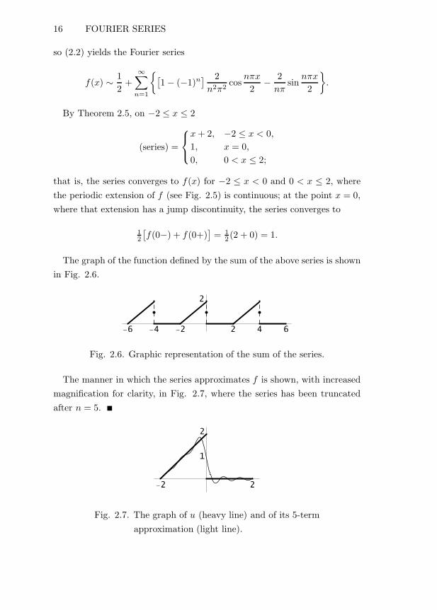
so (2.2) yields the Fourier series
f(x) ∼ 12
+∞∑
n=1
{[1 − (−1)n
] 2n2π2
cosnπx
2− 2nπ
sinnπx
2
}.
By Theorem 2.5, on −2 ≤ x ≤ 2
(series) =
⎧⎨⎩x+ 2, −2 ≤ x < 0,1, x = 0,0, 0 < x ≤ 2;
that is, the series converges to f(x) for −2 ≤ x < 0 and 0 < x ≤ 2, wherethe periodic extension of f (see Fig. 2.5) is continuous; at the point x = 0,where that extension has a jump discontinuity, the series converges to
12
[f(0−) + f(0+)
]= 1
2 (2 + 0) = 1.
The graph of the function defined by the sum of the above series is shownin Fig. 2.6.
2
�6 �4 �2 2 4 6
Fig. 2.6. Graphic representation of the sum of the series.
The manner in which the series approximates f is shown, with increasedmagnification for clarity, in Fig. 2.7, where the series has been truncatedafter n = 5.
2
�2 2
1
Fig. 2.7. The graph of u (heavy line) and of its 5-termapproximation (light line).
FOURIER SINE SERIES 17
2.2. Fourier Sine SeriesFor some classes of functions, series (2.2) has a simpler form.
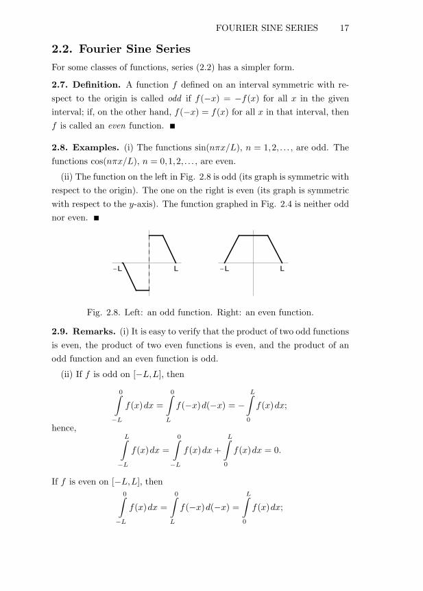
2.7. Definition. A function f defined on an interval symmetric with re-spect to the origin is called odd if f(−x) = −f(x) for all x in the giveninterval; if, on the other hand, f(−x) = f(x) for all x in that interval, thenf is called an even function.
2.8. Examples. (i) The functions sin(nπx/L), n = 1,2, . . . , are odd. Thefunctions cos(nπx/L), n = 0,1,2, . . . , are even.
(ii) The function on the left in Fig. 2.8 is odd (its graph is symmetric withrespect to the origin). The one on the right is even (its graph is symmetricwith respect to the y-axis). The function graphed in Fig. 2.4 is neither oddnor even.
�L L �L L
Fig. 2.8. Left: an odd function. Right: an even function.
2.9. Remarks. (i) It is easy to verify that the product of two odd functionsis even, the product of two even functions is even, and the product of anodd function and an even function is odd.
(ii) If f is odd on [−L,L], then
0∫−L
f(x)dx =
0∫L
f(−x)d(−x) = −L∫
0
f(x)dx;
hence,L∫
−L
f(x)dx =
0∫−L
f(x)dx +
L∫0
f(x)dx = 0.
If f is even on [−L,L], then0∫
−L
f(x)dx =
0∫L
f(−x)d(−x) =
L∫0
f(x)dx;

18 FOURIER SERIES
consequently,L∫
−L
f(x)dx =
0∫−L
f(x)dx +
L∫0
f(x)dx = 2
L∫0
f(x)dx.
(iii) If f is odd, then so is f(x)cos(nπx/L) and, in view of (2.7), (2.8),and (ii) above, we have
an = 0, n = 0,1,2, . . . ;
that is, the Fourier series of an odd function on [−L,L] contains only sineterms. Similarly, if f is even, then, by Remark 2.9(i), f(x)sin(nπx/L) isodd, so (2.9) implies that
bn = 0, n = 1,2, . . . ,
which means that the Fourier series of an even function on [−L,L] has onlycosine terms, including the constant term.
Remark 2.9(iii) implies that if f is defined on [0,L], then it can be ex-panded in a Fourier sine series. Let f be the function whose graph is shownin Fig. 2.9.
L
Fig. 2.9. f(x), 0 ≤ x ≤ L.
We construct the odd extension of f from (0,L] to [−L,L] by settingf(−x) = −f(x) for all x in [−L,L], x �= 0, and f(0) = 0 (see Fig. 2.10).
�L L
Fig. 2.10. f(−x) = −f(x), −L ≤ x ≤ L.

FOURIER SINE SERIES 19
Next, we construct the periodic extension with period 2L of this oddfunction from (−L,L] to R, by requiring that f(x+ 2L) = f(x) for all x inR (see Fig. 2.11).
�3L �2L �L L 2L 3L
Fig. 2.11. f(x+ 2L) = f(x) for all x in R.
Finally, we construct the Fourier (sine) series of this last function, whichis of the form
f(x) ∼∞∑
n=1
bn sinnπx
L,
where, according to Remarks 2.9(ii),(iii) and formula (2.9), the coefficientsare given by
bn =2L
L∫0
f(x)sinnπx
Ldx, n = 1,2, . . . . (2.10)
2.10. Example. Consider the function
f(x) = 1 − x, 0 ≤ x ≤ 1,
graphed in Fig. 2.12.
1
1
Fig. 2.12. f(x), 0 ≤ x ≤ 1.
As explained above, the odd extension of this function to [−1,1] is definedby f(−x) = −f(x) for all x in [−1,1], x �= 0, and f(0) = 0, and is shown inFig. 2.13.

20 FOURIER SERIES
1
�1
�1 1
Fig. 2.13. f(−x) = −f(x), −1 ≤ x ≤ 1.
The periodic extension to R, of period 2L = 2, of the function in Fig. 2.13,defined by f(x+ 2) = f(x) for all x in R, is shown in Fig. 2.14.
1
�1
�3 �2 �1 1 2 3
Fig. 2.14. f(x+ 2) = f(x) for all x in R.
Using (2.10) with L = 1 and integration by parts, we find that
bn = 2
1∫0
(1 − x)sin(nπx)dx =2nπ
, n = 1,2, . . . ;
hence,
f(x) ∼∞∑
n=1
2nπ
sin(nπx).
By Theorem 2.5, for 0 ≤ x ≤ 1,
(series) ={
0, x = 0,1 − x, 0 < x ≤ 1;
that is, the series converges to f(x) for 0 < x ≤ 1, where the periodicextension of f to R is continuous, and to
12
[f(0−) + f(0+)
]= 1
2 (−1 + 1) = 0
at x = 0, where the periodic extension has a jump discontinuity.

FOURIER COSINE SERIES 21
2.3. Fourier Cosine Series
By Remark 2.9(iii), a function defined on [0,L] can also be expanded in aFourier cosine series. The construction is similar to that of a Fourier sineseries.
Let f be a function defined on [0,L] (see Fig. 2.15).
L
Fig. 2.15. f(x), 0 ≤ x ≤ L.
We extend f to an even function on [−L,L] by setting f(−x) = f(x) forall x in [−L,L] (see Fig. 2.16).
�L L
Fig. 2.16. f(−x) = f(x), −L ≤ x ≤ L.
Next, we construct the periodic extension of this even function from(−L,L] to R, of period 2L, which is defined by f(x + 2L) = f(x) for all xin R (see Fig. 2.17).
�3L �L L 3L
Fig. 2.17. f(x+ 2L) = f(x) for all x in R.
Finally, we write the Fourier (cosine) series of this last function, which isof the form
f(x) ∼ 12a0 +
∞∑n=1
an cosnπx
L,

22 FOURIER SERIES
where, according to (2.7), (2.8), and Remark 2.9(ii),
a0 =2L
L∫0
f(x)dx,
an =2L
L∫0
f(x)cosnπx
Ldx, n = 1,2, . . . .
(2.11)
As noticed earlier, the first equality (2.11) is covered by the second one ifwe let n = 0,1,2, . . . .
2.11. Example. Consider the function
f(x) = 1 − x, 0 ≤ x ≤ 1,
graphed in Fig. 2.18.
1
1
Fig. 2.18. f(x), 0 ≤ x ≤ 1.
The even extension of f to [−1,1], defined by f(−x) = f(x) for all x in[−1,1], is shown in Fig. 2.19.
1
�1 1
Fig. 2.19. f(−x) = f(x), −1 ≤ x ≤ 1.
The periodic extension of period 2L = 2 of this even function to R, whichis defined by f(x+ 2) = f(x) for all x in R, is shown in Fig. 2.20.
1
�3 �1 1 3
Fig. 2.20. f(x+ 2) = f(x) for all x in R.

CONVERGENCE AND DIFFERENTIATION 23
By (2.11) with L = 1 and integration by parts,
a0 = 2
1∫0
f(x)dx = 2
1∫0
(1 − x)dx = 1,
an = 2
1∫0
f(x)cos(nπx)dx = 2
1∫0
(1 − x)cos(nπx)dx
=[1 − (−1)n
] 2n2π2
, n = 1,2, . . . ,
so the Fourier cosine series of f is
f(x) ∼ 12
+∞∑
n=1
[1 − (−1)n
] 2n2π2
cos(nπx).
By Theorem 2.5,(series) = 1 − x for 0 ≤ x ≤ 1,
because the periodic extension of f to R is continuous everywhere.
2.4. Convergence and Differentiation
There are several important points that need to be made at this stage.
2.12. Remarks. (i) It is obvious that a function f defined on [0,L] canbe expanded in a full Fourier series, or in a sine series, or in a cosine series.While the last two are unique to the function, the first one is not: sincethe full Fourier series requires no symmetry, we may extend f from [0,L] to[−L,L] in infinitely many ways. We usually choose the type of series thatseems to be the most appropriate for the problem. A function defined on[−L,L] can be expanded, in general, only in a full Fourier series.
(ii) Earlier we saw that we cannot automatically use the equality signbetween a function f and its Fourier series. According to Theorem 2.5, fora full series we can do so at all the points in [−L,L] where f is continuous;we can also do it at x = −L and x = L provided that f is continuous at thesepoints from the right and from the left, respectively, and f(−L) = f(L).For a sine series, this can be done at x = L if f is continuous there fromthe left and f(L) = 0. For a cosine series this is always possible if f iscontinuous from the left at x = L. Similar arguments can be used for

24 FOURIER SERIES
the sine and cosine series at x = 0. In what follows we work exclusivelywith piecewise smooth functions; therefore, to avoid cumbersome notationand possible confusion, we will use the equality sign in all circumstances,assuming tacitly that equality is understood in the sense of Theorem 2.5,Remark 2.4(ii), and the above comments.
In practical applications we often need to differentiate Fourier series termby term. Consequently, it is important to know when this operation maybe performed.
2.13. Theorem. (i) If f is continuous on [−L,L], f(−L) = f(L), andf ′ is piecewise smooth on [−L,L], then the full Fourier series of f can bedifferentiated term by term and the resulting series is the Fourier seriesof f ′, which converges to f ′(x) at all x where f ′′(x) exists.
(ii) If f is continuous on [0,L], f(0) = f(L) = 0, and f ′ is piecewisesmooth on [0,L], then the Fourier sine series of f can be differentiated termby term and the resulting series is the Fourier cosine series of f ′, whichconverges to f ′(x) at all x where f ′′(x) exists.
(iii) If f is continuous on [0,L] and f ′ is piecewise smooth on [0,L], thenthe Fourier cosine series of f can be differentiated term by term and theresulting series is the Fourier sine series of f ′, which converges to f ′(x) atall x where f ′′(x) exists.
2.14. Remark. In the PDE problems that we discuss in the rest of thebook, the conditions laid down in Theorem 2.13 will always be satisfied andwe will formally differentiate the corresponding Fourier series term by termwithout explicit mention of these conditions.
Exercises
In (1)–(16) construct the full Fourier series of the given function f . In eachcase discuss the convergence of the series on the interval [−L,L] where f isdefined and sketch the function to which the series converges pointwise onthe interval [−3L,3L].
(1) f(x) ={
1, −1 ≤ x ≤ 0,0, 0 < x ≤ 1.

EXERCISES 25
(2) f(x) ={
0, −π ≤ x ≤ 0,−3, 0 < x ≤ π.
(3) f(x) ={−2, −1 ≤ x ≤ 0,
3, 0 < x ≤ 1.
(4) f(x) ={
1, −π/2 ≤ x ≤ 0,2, 0 < x ≤ π/2.
(5) f(x) = x+ 1, −1 ≤ x ≤ 1.
(6) f(x) = 1 − 2x, −2 ≤ x ≤ 2.
(7) f(x) ={−1, −2 ≤ x ≤ 0,
2 − x, 0 < x ≤ 2.
(8) f(x) ={
1 + 2x, −1/2 ≤ x ≤ 0,4, 0 < x ≤ 1/2.
(9) f(x) ={x, −1 ≤ x ≤ 0,2x− 1, 0 < x ≤ 1.
(10) f(x) ={x− 1, −π ≤ x ≤ 0,2x+ 1, 0 < x ≤ π.
(11) f(x) = x2 − 2x+ 3, −1 ≤ x ≤ 1.
(12) f(x) ={x2, −1 ≤ x ≤ 0,1 + 2x, 0 < x ≤ 1.
(13) f(x) = ex, −2 ≤ x ≤ 2.
(14) f(x) ={
1, −π/2 ≤ x ≤ 0,sinx, 0 < x ≤ π/2.
(15) f(x) ={
0, −2 ≤ x ≤ −1,1 + x, −1 < x ≤ 2.
(16) f(x) ={
3, −π ≤ x ≤ π/2,1, π/2 < x ≤ π.
In (17)–(30) construct the Fourier sine series and the Fourier cosine seriesof the given function f . In each case discuss the convergence of the serieson the interval [0,L] where f is defined and sketch the functions to whichthe series converge pointwise on [−3L,3L].
(17) f(x) ={
0, 0 ≤ x ≤ 1,1, 1 < x ≤ 2.
(18) f(x) ={
2, 0 ≤ x ≤ π,0, π < x ≤ 2π.
26 FOURIER SERIES
(19) f(x) ={
1, 0 ≤ x ≤ 1,−1, 1 < x ≤ 2.
(20) f(x) ={−2, 0 ≤ x ≤ π/2,
3, π/2 < x ≤ π.
(21) f(x) = 2 − x, 0 ≤ x ≤ 1.
(22) f(x) = 3x+ 1, 0 ≤ x ≤ 2π.
(23) f(x) ={x, 0 ≤ x ≤ 1,−2, 1 < x ≤ 2.
(24) f(x) ={
2x− 1, 0 ≤ x ≤ 1,2x+ 1, 1 < x ≤ 2.
(25) f(x) ={
2 + x, 0 ≤ x ≤ 1,1 − x, 1 < x ≤ 2.
(26) f(x) = x2 + x− 1, 0 ≤ x ≤ 2.
(27) f(x) ={x+ 1, 0 ≤ x ≤ 1,x2 − 2x, 1 < x ≤ 2.
(28) f(x) = 1 + ex, 0 ≤ x ≤ 1.
(29) f(x) = x+ sinx, 0 ≤ x ≤ π.
(30) f(x) ={
cosx, 0 ≤ x ≤ π/2,−1, π/2 < x ≤ π.

Chapter 3Sturm–Liouville Problems
There is a class of problems involving second-order ODEs, which plays anessential role in the solution of partial differential equations. Below wepresent the main results concerning such problems, thus laying the founda-tion for the methods of separation of variables and eigenfunction expansiondeveloped in Chapters 5 and 7.
3.1. Regular Sturm–Liouville Problems
To avoid complicated notation, in what follows we denote intervals generi-cally by I, regardless of whether they are closed, open, or half-open, finiteor infinite. Specific intervals are described either in terms of their endpointsor by means of inequalities. The functions defined on such intervals areassumed to be integrable on them.
3.1. Definition. Let X be a space of functions defined on an interval I.A linear differential operator L acting on X is called symmetric on X if∫
I
[f1(x)(Lf2)(x) − f2(x)(Lf1)(x)
]dx = 0
for any functions f1 and f2 in X .
3.2. Example. Consider the space X of functions that are twice continu-ously differentiable on [0,1] and equal to zero at x = 0 and x = 1. If L isthe linear operator defined by L ≡ d2/dx2, then, using integration by parts,we find that for any f1 and f2 in X ,
1∫0
[f1(Lf2) − f2(Lf1)
]dx =
1∫0
(f1f ′′2 − f2f
′′1 )dx
=[f1f
′2
]10−
1∫0
f ′1f
′2dx− [
f2f′1
]10
+
1∫0
f ′1f
′2dx = 0.
Hence, L is symmetric on X .

28 STURM–LIOUVILLE PROBLEMS
3.3. Remark. An operator may be symmetric on a space of functions butnot on another. If no restriction is imposed on the values at x = 0 andx = 1 of the functions in Example 3.2, then L is not symmetric on the newspace X .
3.4. Definition. Let σ be a function defined on I, with the property thatσ(x) > 0 for all x in I. Two functions f1 and f2, also defined on I, arecalled orthogonal with weight σ on I if∫
I
f1(x)f2(x)σ(x)dx = 0.
If σ(x) = 1, then f1 and f2 are simply called orthogonal. A set of functionsthat are pairwise orthogonal on I is called an orthogonal set.
3.5. Example. The functions f1(x) = 1 and f2(x) = 9x−5 are orthogonalwith weight σ(x) = x+ 1 on [0,1] since
1∫0
(9x− 5)(x+ 1)dx =
1∫0
(9x2 + 4x− 5)dx = 0.
Alternatively, we can say that the functions f1(x) = x+1 and f2(x) = 9x−5are orthogonal on [0,1].
3.6. Example. The functions sin(3x) and cos(2x) are orthogonal on theinterval [−π,π] because
π∫−π
sin(3x)cos(2x)dx =
π∫−π
12
[sin(5x) + sinx
]dx = 0.
3.7. Definition. Let L be a linear differential operator acting on a spaceX of functions defined on (a,b). An equation of the form
(Lf)(x) + λσ(x)f(x) = 0, a < x < b, (3.1)
where λ is a (real) parameter and σ is a given function such that σ(x) > 0for all x in (a,b), is called an eigenvalue problem. The numbers λ for which(3.1) has nonzero solutions in X are called eigenvalues; the correspondingnonzero solutions are called eigenfunctions.

REGULAR PROBLEMS 29
3.8. Theorem. If the operator L of the eigenvalue problem (3.1) is sym-metric, then
(i) all the eigenvalues λ are real;
(ii) the eigenvalues form an infinite sequence λ1 < λ2 < · · · < λn < · · ·such that λn → ∞ as n→ ∞;
(iii) eigenfunctions associated with distinct eigenvalues are orthogonalwith weight σ on (a,b).
3.9. Definition. Let [a,b] be a finite interval, let p, q, and σ be real-valuedfunctions, and let κ1, κ2, κ3, and κ4 be real numbers such that
(i) p is continuously differentiable on [a,b] and p(x) > 0 for all x in [a,b];(ii) q and σ are continuous on [a,b] and σ(x) > 0 for all x in [a,b];(iii) κ1, κ2 are not both zero and κ3, κ4 are not both zero.
An eigenvalue problem of the form
[p(x)f ′(x)
]′ + q(x)f(x) + λσ(x)f(x) = 0, a < x < b, (3.2)
with the boundary conditions (BCs)
κ1f(a) + κ2f′(a) = 0, (3.3)
κ3f(b) + κ4f′(b) = 0, (3.4)
is called a regular Sturm–Liouville (S–L) eigenvalue problem.
3.10. Example. The choice
p(x) = 1, q(x) = 0, σ(x) = 1,
κ1 = 1, κ2 = 0, κ3 = 1, κ4 = 0, a = 0, b = L
generates the regular S–L problem
f ′′(x) + λf(x) = 0, 0 < x < L,
f(0) = 0, f(L) = 0.
3.11. Example. If p, q, σ, a, and b are as in Example 3.10 but κ1 = 0,κ2 = 1, κ3 = 0, and κ4 = 1, then we have the regular S–L problem
f ′′(x) + λf(x) = 0, 0 < x < L,
f ′(0) = 0, f ′(L) = 0.

30 STURM–LIOUVILLE PROBLEMS
3.12. Example. Taking p, q, σ, a, and b as in Example 3.10 and the coef-ficients
κ1 = 1, κ2 = 0, κ3 = h, κ4 = 1,
we obtain the regular S–L problem
f ′′(x) + λf(x) = 0, 0 < x < L,
f(0) = 0, f ′(L) + hf(L) = 0.
3.13. Example. The eigenvalue problem
f ′′(x) + 2f ′(x) + λf(x) = 0, 0 < x < 1,
f(0) = 0, f(1) = 0
is, in fact, a regular Sturm–Liouville problem. Adopting an “integratingfactor”-type technique and using the coefficient of f ′, we choose the func-tions
p(x) = σ(x) = exp{∫
2dx}
= e2x, q(x) = 0.
These functions satisfy the requirements of Definition 3.9 and, as can im-mediately be verified, the equality
(e2xf ′(x)
)′ + λe2xf(x) = 0, 0 < x < 1,
is equivalent to the given equation.
3.14. Theorem. The operator
Lf = (pf ′)′ + qf (3.5)
defined by the left-hand side in (3.2) and acting on a space X of functionssatisfying (3.3) and (3.4) is symmetric on X .
Proof. Suppose, for simplicity, that κ1 �= 0 and κ4 �= 0. Then, by (3.3)and (3.4), any function f in X satisfies
f(a) = −κ2
κ1f ′(a), f ′(b) = −κ3
κ4f(b).

REGULAR PROBLEMS 31
Consequently, using (3.5) and integration by parts, we find that for any f1and f2 in X ,
b∫a
[f1(Lf2) − f2(Lf1)
]dx
=
b∫a
{f1
[(pf ′
2)′ + qf2
] − f2[(pf ′
1)′ + qf1
]}dx
=[f1(pf ′
2)]b
a−
b∫a
pf ′2f
′1dx− [
f2(pf ′1)
]b
a+
b∫a
pf ′1f
′2dx
= p(b)[f1(b)f ′
2(b) − f2(b)f ′1(b)
] − p(a)[f1(a)f ′
2(a) − f2(a)f ′1(a)
]
= p(b)[− κ3
κ4f1(b)f2(b) +
κ3
κ4f2(b)f1(b)
]
− p(a)[− κ2
κ1f ′1(a)f
′2(a) +
κ2
κ1f ′2(a)f
′1(a)
]= 0,
as required. All other combinations of nonzero constants κ1, κ2, κ3, and κ4
are treated similarly.
3.15. Corollary. The eigenvalues and eigenfunctions of a regular Sturm–Liouville problem have all the properties listed in Theorem 3.8.
Before actually computing the eigenvalues and eigenfunctions of specificSturm–Liouville problems, we derive a very useful formula relating thesequantities. Multiplying (3.2) by f and integrating over (a,b), we easily seethat
0 =
b∫a
[f(pf ′)′ + qf2
]dx+ λ
b∫a
σf2dx
=
b∫a
[(pff ′)′ − p(f ′)2 + qf2
]dx + λ
b∫a
σf2dx
=[pff ′]b
a−
b∫a
[p(f ′)2 − qf2
]dx+ λ
b∫a
σf2dx.
32 STURM–LIOUVILLE PROBLEMS
Since f is an eigenfunction (nonzero solution) and σ(x) > 0 for a < x < b,the coefficient of λ in the last term is strictly positive. Hence, we can solvefor λ and obtain
λ =
b∫a
[p(f ′)2 − qf2
]dx− [
pff ′]b
a
b∫a
σf2 dx
. (3.6)
This expression is known as the Rayleigh quotient.
3.16. Example. For the regular S–L problem considered in Example 3.10we have
b∫a
[p(x)(f ′)2(x) − q(x)f2(x)
]dx =
L∫0
(f ′)2(x)dx ≥ 0,
[p(x)f(x)f ′(x)
]b
a=
[f(x)f ′(x)
]L
0= 0,
b∫a
σ(x)f2(x)dx =
L∫0
f2(x)dx > 0,
so (3.6) yields
λ =
L∫0
(f ′)2(x)dx
L∫0
f2(x)dx≥ 0. (3.7)
It is clear that λ = 0 if and only if f ′(x) = 0 on [0,L], which means thatf(x) = const. But this is unacceptable because, according to the BCs, theonly constant solution is the zero solution. Consequently, λ > 0, and thegeneral solution of the equation in Example 3.10 is
f(x) = C1 cos(√λx
)+ C2 sin
(√λx
), C1, C2 = const. (3.8)
Using the condition f(0) = 0, we find that C1 = 0. Then the conditionf(L) = 0 leads to
C2 sin(√λL
)= 0.

REGULAR PROBLEMS 33
We cannot have C2 = 0 because this would imply that f = 0 and we areseeking nonzero solutions; therefore, we must conclude that sin
(√λL
)= 0,
from which we obtain√λL = nπ, n = 1,2, . . . , or
λn =(nπ
L
)2
, n = 1,2, . . . .
These are the eigenvalues of the problem. The corresponding eigenfunctions(nonzero solutions) are
fn(x) = sinnπx
L, n = 1,2, . . . .
For convenience, we have taken C2 = 1; any other nonzero value of C2 wouldsimply produce a multiple of sin(nπx/L).
It is easy to see that the properties in Theorem 3.8 are satisfied. Theorthogonality of the eigenfunctions on [0,L] follows immediately from (2.5)since the integrand is an even function.
3.17. Example. The same technique is used to compute the eigenvaluesand eigenfunctions of the S–L problem in Example 3.11. Inequality (3.7)remains valid, but now we cannot reject the case λ = 0 since the functionsf(x) = c = const corresponding to it satisfy both BCs. Taking, say, c = 1/2,we conclude that the problem has the eigenvalue-eigenfunction pair
λ0 = 0, f0(x) = 1/2.
As in Example 3.16, for λ > 0 the general solution of the equation is(3.8), so
f ′(x) = −C1
√λsin
(√λx
)+ C2
√λcos
(√λx
).
The condition f ′(0) = 0 immediately yields C2 = 0; therefore, f ′(L) = 0implies that
C1
√λ sin
(√λL
)= 0.
Since we want nonzero solutions, it follows that sin(√λL
)= 0. This means
that√λL = nπ, n = 1,2, . . . , so, by (3.8) with C2 = 0 and C1 = 1, the
eigenvalue-eigenfunction pairs are
λn =(nπ
L
)2
, fn(x) = cosnπx
L, n = 1,2, . . . .

34 STURM–LIOUVILLE PROBLEMS
We remark that the full set of eigenvalues and eigenfunctions of the problemcan be written as above, but with n = 0,1,2, . . . .
Once again, we note that the eigenvalues and eigenfunctions satisfy theproperties in Theorem 3.8. The orthogonality of the latter on [0,L] followsfrom the first formula (2.3) and (2.4).
3.18. Example. Suppose that h > 0 in the S–L problem considered inExample 3.12. Then, writing the second BC of that problem in the formf ′(L) = −hf(L), we see that
[p(x)f(x)f ′(x)
]b
a=
[f(x)f ′(x)
]L
0= f(L)f ′(L) − f(0)f ′(0) = −hf2(L).
Consequently, (3.6) yields
λ =
L∫0
(f ′)2(x)dx + hf2(L)
L∫0
f2(x)dx≥ 0,
with λ = 0 if and only if f ′(x) = 0 on [0,L] and f(L) = 0. But this impliesthat f = 0, which is not acceptable. Hence, the eigenvalues of this S–Lproblem are positive. To find them, we note that the general solution ofthe equation is again given by (3.8) and that the condition f(0) = 0 leadsto C1 = 0. Using the second BC, namely, f ′(L) + hf(L) = 0, we arrive at
C2
[√λ cos
(√λL
)+ hsin
(√λL
)]= 0.
For nonzero solutions we must have C2 �= 0; in other words,
√λcos
(√λL
)+ hsin
(√λL
)= 0.
Since cos(√λL
) �= 0 (otherwise sin(√λL
)would be zero as well, which is
impossible), we can divide the above equality by cos(√λL
)and conclude
that λ must be a solution of the transcendental equation
tan(√λL
)= −
√λ
h= − 1
hL
(√λL
).
Setting√λL = ζ, we see that ζ is given by the points of intersection of the
graphs of the functions y = tanζ and y = −ζ/(hL).

REGULAR PROBLEMS 35
Π�2 3Π�2 5Π�2Ζ1 Ζ2
Fig. 3.1. The graphs of y = tanζ (heavy line) and y =−ζ/(hL) (light line).
As Fig. 3.1 shows, there are countably many such points ζn, so thisS–L problem has an infinite sequence of positive eigenvalues
λn =(ζnL
)2
, n = 1,2, . . . , λn → ∞ as n→ ∞,
with corresponding eigenfunctions (given by (3.8) with C1 = 0 and C2 = 1)
fn(x) = sin(√
λnx)
= sinζnx
L, n = 1,2, . . . .
By Theorem 3.8(iii), the set{fn
}∞n=1
is orthogonal on [0,L].
3.19. Example. For the S–L problem introduced in Example 3.13 we usea slightly modified approach. Here the roots of the characteristic equations2 + 2s+ λ = 0 are
s1 = −1 +√
1 − λ, s2 = −1 −√1 − λ.
Since the nature of the roots changes according as λ < 1, λ = 1, or λ > 1,we consider these cases individually.

36 STURM–LIOUVILLE PROBLEMS
(i) If λ < 1, then 1 − λ > 0; hence, s1 and s2 are real and distinct, andthe general solution of the equation is
f(x) = C1es1x + C2e
s2x, C1, C2 = const.
Using the conditions f(0) = 0 and f(1) = 0, we arrive at
C1 + C2 = 0, C1es1 + C2e
s2 = 0.
Since s1 �= s2, this system has only the solution C1 = C2 = 0; consequently,f = 0, and we conclude that there are no eigenvalues λ < 1.
(ii) If λ = 1, then
f(x) = (C1 + C2x)e−x, C1, C2 = const.
The condition f(0) = 0 yields C1 = 0, while f(1) = 0 gives C2e−1 = 0,
which means that C2 = 0. This generates f = 0, so λ = 1 is not aneigenvalue.
(iii) If λ > 1, then the general solution of the equation is
f(x) = e−x[C1 cos
(√λ− 1x
)+ C2 sin
(√λ− 1x
)], C1, C2 = const.
Since f(0) = 0, we find that C1 = 0, and from the other condition, f(1) = 0,it follows that
C2e−1 sin
√λ− 1 = 0.
For nonzero solutions we must have
sin√λ− 1 = 0;
in other words, √λ− 1 = nπ, n = 1,2, . . . .
This implies that the eigenvalues of the problem are
λn = n2π2 + 1, n = 1,2, . . . ,
with corresponding eigenfunctions
fn(x) = e−x sin(√
λn − 1x)
= e−x sin(nπx), n = 1,2, . . . .
Regular Sturm–Liouville problems have two important additional prop-erties.

REGULAR PROBLEMS 37
3.20. Theorem. (i) Only one linearly independent eigenfunction fn existsfor each eigenvalue λn, n = 1,2, . . . .
(ii) The set{fn
}∞n=1
of eigenfunctions is complete; that is, any piece-wise smooth function u on [a,b] has a unique generalized Fourier series (oreigenfunction) expansion of the form
u(x) ∼∞∑
n=1
cnfn(x), a ≤ x ≤ b, (3.9)
which converges pointwise to 12
[u(x−)+u(x+)
]for a ≤ x ≤ b (in particular,
to u(x) if u is continuous at x).
3.21. Remarks. (i) The coefficients cn are computed by means of the prop-erties mentioned in Theorem 3.20(i) and Theorem 3.8(iii). Thus, treating(3.9) formally as an equality, multiplying it by fm(x)σ(x), and integratingover [a,b], we obtain
b∫a
u(x)fm(x)σ(x)dx =∞∑
n=1
cn
b∫a
fn(x)fm(x)σ(x)dx
= cm
b∫a
f2m(x)σ(x)dx.
Replacing m by n, we can now write
cn =
b∫a
u(x)fn(x)σ(x)dx
b∫a
f2n(x)σ(x)dx
, n = 1,2, . . . . (3.10)
The denominator in (3.10) cannot be zero for any n since the fn are nonzerosolutions of (3.2)–(3.4) and σ(x) > 0.
(ii) In the case of the S–L problems discussed in Examples 3.10 and 3.16,and in Examples 3.11 and 3.17, expansion (3.9) coincides, respectively, withthe Fourier sine and cosine series of u, and (3.10) yields formulas (2.10) and(2.11). (For the problem in Examples 3.11 and 3.17, n = 0,1,2, . . . .)
(iii) Using the method in Example 3.19, we can show that the eigenvaluesand eigenfunctions of the more general regular S–L problem

38 STURM–LIOUVILLE PROBLEMS
f ′′(x) + af ′(x) + bf(x) + λcf(x) = 0, 0 < x < L,
f(0) = 0, f(L) = 0,
where a, b, and c > 0 are constants, are, respectively,
λn =14c
(4n2π2
L2+ a2 − 4b
), fn(x) = e−(a/2)x sin
nπx
L, n = 1,2, . . . .
3.22. Example. Suppose that we want to expand the function
u(x) = x+ 1, 0 ≤ x ≤ 1,
in the eigenfunctions of the regular S–L problem discussed in Examples3.12 and 3.18 with L = h = 1. The first five positive roots of the equationtanζ = −ζ mentioned in the latter are, approximately,
ζ1 = 2.0288, ζ2 = 4.9132, ζ3 = 7.9787, ζ4 = 11.0855, ζ5 = 14.2074.
Then, using (3.10) with σ(x) = 1, we find the approximate coefficients
c1 = 1.9184, c2 = 0.1572, c3 = 0.3390, c4 = 0.1307, c5 = 0.1696,
so (3.9) takes the form
u(x) ∼ 1.9184sin(2.0288x) + 0.1572sin(4.9132x) + 0.3390sin(7.9787x)
+ 0.1307sin(11.0855x) + 0.1696sin(14.2074x) + · · · .
3.23. Example. Consider the function
u(x) = e−x, 0 ≤ x ≤ 1.
If fn are the eigenfunctions of the regular S–L problem discussed in Exam-ples 3.13 and 3.19, that is,
fn(x) = e−x sin(nπx), n = 1,2, . . . ,
then (3.10) with σ(x) = e2x yields the coefficients
cn =[1 − (−1)n
] 2nπ
, n = 1,2, . . . ,
so expansion (3.9) is
u(x) ∼∞∑
n=1
[1 − (−1)n
] 2nπ
e−x sin(nπx).

OTHER PROBLEMS 39
3.2. Other Problems
Many important Sturm–Liouville problems are not regular.
3.24. Definition. With the notation in Definition 3.9, an eigenvalue prob-lem that consists in solving equation (3.2) with the conditions
f(a) = f(b), f ′(a) = f ′(b) (3.11)
is called a periodic Sturm–Liouville problem.
3.25. Remark. It can be shown that the differential operator L intro-duced in (3.5) is also symmetric on the new space of functions defined byconditions (3.11), so Theorem 3.8 is again applicable. However, in contrastto regular S–L problems, here we may have two linearly independent eigen-functions for the same eigenvalue. Nevertheless, we can always choose apair of eigenfunctions that are orthogonal with weight σ on [a,b]. For sucha choice, Theorem 3.20(ii) remains valid.
3.26. Example. Consider the periodic Sturm–Liouville problem wherep(x) = 1, q(x) = 0, σ(x) = 1, a = −L, and b = L, L > 0; that is,
f ′′(x) + λf(x) = 0, −L < x < L,
f(−L) = f(L), f ′(−L) = f ′(L).
Using the Rayleigh quotient argument and the above BCs, we arrive againat inequality (3.7). We accept the case λ = 0 since, as in Example 3.17, thecorresponding constant solutions satisfy both BCs; therefore, the problemhas the eigenvalue-eigenfunction pair
λ0 = 0, f0(x) = 12 .
For λ > 0, the general solution of the equation is
f(x) = C1 cos(√λx
)+ C2 sin
(√λx
), C1, C2 = const,
with derivative
f ′(x) = −C1
√λsin
(√λx
)+ C2
√λcos
(√λx
).

40 STURM–LIOUVILLE PROBLEMS
From the BCs and the fact that cos(−α) = cosα and sin(−α) = −sinα itfollows that C1 and C2 satisfy the system
C1 cos(√λL
) − C2 sin(√λL
)= C1 cos
(√λL
)+ C2 sin
(√λL
),
C1 sin(√λL
)+ C2 cos
(√λL
)= −C1 sin
(√λL
)+ C2 cos
(√λL
),
which reduces to
C1 sin(√λL
)= 0, C2 sin
(√λL
)= 0.
Since we want nonzero solutions, we cannot have sin(√λL
) �= 0 becausethis would imply C1 = C2 = 0, that is, f = 0; hence, sin
(√λL
)= 0. As we
have seen in previous examples, this yields the eigenvalues
λn =(nπ
L
)2
, n = 1,2, . . . .
Given that both C1 and C2 remain arbitrary, from the general solution wecan extract (by taking C1 = 1, C2 = 0 and then C1 = 0, C2 = 1) for everyλn the two linearly independent eigenfunctions
f1n(x) = cosnπx
L, f2n(x) = sin
nπx
L, n = 1,2, . . . ,
which, as seen in Chapter 2, are orthogonal on [−L,L]. Expansion (3.9) inthis case becomes
u(x) ∼ 12c0 +
∞∑n=1
[c1nf1n(x) + c2nf2n(x)
]
=12c0 +
∞∑n=1
(c1n cos
nπx
L+ c2n sin
nπx
L
),
which we recognize as the full Fourier series of u. The coefficients c0, c1n,and c2n, computed by means of (3.10) with σ(x) = 1, a = −L, b = L, andn = 0,1,2, . . . (to allow for the additional eigenfunction f0), coincide withthose given by (2.7)–(2.9).
3.27. Definition. An eigenvalue problem involving equation (3.2) is calleda singular Sturm–Liouville problem if it exhibits one or more of the followingfeatures:

BESSEL FUNCTIONS 41
(i) p(a) = 0 or p(b) = 0 or both;
(ii) any of p(x), q(x), and σ(x) becomes infinite as x→ a+ or as x→ b−or both;
(iii) the interval (a,b) is infinite at a or at b or at both.
3.28. Remark. In the case of a singular Sturm–Liouville problem, somenew boundary conditions need to be chosen to ensure that the operator Ldefined by (3.5) remains symmetric. For example, if p(a) = 0 but p(b) �= 0,then we may require f(x) and f ′(x) to remain bounded as x → a+ andto satisfy (3.4). If the interval where the equation holds is of the form(a,∞), then we may require f(x) and f ′(x) to be bounded as x → ∞ andto satisfy (3.3). Other types of boundary conditions, dictated by analyticand/or physical necessity, may also be considered.
3.29. Example. The eigenvalue problem
(x2 + 1)f ′′(x) + 2xf ′(x) + (λ − x)f(x) = 0, x > 1,
f ′(1) = 0, f(x), f ′(x) bounded as x→ ∞,
is a singular S–L problem: the ODE can be written in the form (3.2) withp(x) = x2 + 1, q(x) = −x, σ(x) = 1, and (a,b) = (1,∞), and the boundaryconditions are of the type indicated in the latter part of Remark 3.28.
A number of singular S–L problems occurring in the study of mathemat-ical models give rise to important classes of functions. We discuss some ofthem explicitly.
3.3. Bessel Functions
Consider the singular S–L problem
x2f ′′(x) + xf ′(x) + (λx2 −m2)f(x) = 0, 0 < x < a, (3.12)
f(x), f ′(x) bounded as x→ 0+, f(a) = 0, (3.13)
where a is a given positive number and m is a nonnegative integer. Writing(3.12) in the form [
xf ′(x)]′ − m2
xf(x) + λxf(x) = 0,
we verify that this is (3.2) with p(x) = x, q(x) = −m2/x, and σ(x) = x.

42 STURM–LIOUVILLE PROBLEMS
First, we consider the case m = 0, when q = 0 and (3.12) reduces to
xf ′′(x) + f ′(x) + λxf(x) = 0, 0 < x < a.
Taking (3.13) into account, we see that
p(x)(f ′)2(x) − q(x)f2(x) = x(f ′)2(x) ≥ 0, 0 < x < a,[p(x)f(x)f ′(x)
]a
0=
[xf(x)f ′(x)
]a
0= af(a)f ′(a) − lim
x→0+xf(x)f ′(x) = 0;
consequently, according to the Rayleigh quotient (3.6),
λ =
a∫0
x(f ′)2(x)dx
a∫0
xf2(x)dx≥ 0.
In fact, as this formula shows, we have λ = 0 if and only if f ′(x) = 0,0 < x ≤ a; that is, if and only if f(x) = const. But this is impossible, sincethe boundary condition f(a) = 0 would imply that f is the zero solution,which contradicts the definition of an eigenfunction. We must thereforeconclude that λ > 0.
Now let m ≥ 1. Multiplying (3.12) by f(x) and integrating from 0 to a,we arrive at
a∫0
[x2f ′′(x)f(x) + xf ′(x)f(x) + λx2f2(x) −m2f2(x)
]dx = 0. (3.14)
Integration by parts, the interpretation of f(x) and f ′(x) at x = 0 in thelimiting sense as above, and (3.13) yield the equalities
a∫0
xf ′(x)f(x)dx =
a∫0
12x(f2(x))′ dx =
12
[xf2(x)
]a
0− 1
2
a∫0
f2(x)dx
= −12
∫ a
0
f2(x)dx,
a∫0
x2f ′′(x)f(x)dx =[x2f ′(x)f(x)
]a
0−
a∫0
[x2(f ′(x))2 + 2xf ′(x)f(x)
]dx
= −a∫
0
[x2(f ′(x))2 − f2(x)
]dx,

BESSEL FUNCTIONS 43
which, replaced in (3.14), lead to
λ =
a∫0
[x2(f ′(x))2 +
(m2 − 1
2
)f2(x)
]dx
a∫0
x2f2(x)dx≥ 0.
The same argument used for m = 0 rules out the value λ = 0; hence, λ > 0.Let ξ =
√λx and f(x) = f
(ξ/√λ
)= g(ξ). By the chain rule,
f ′(x) =√λg′(ξ), f ′′(x) = λg′′(ξ),
and (3.12) becomes
ξ2g′′(ξ) + ξg′(ξ) + (ξ2 −m2)g(ξ) = 0, (3.15)
which is Bessel’s equation of order m. Two linearly independent solutionsof this equation are the Bessel functions of the first and second kind andorder m denoted by Jm and Ym.
3.30. Remarks. (i) For m ≥ 1, the Jm satisfy the recurrence relations
Jm−1(x) + Jm+1(x) = (2m/x)Jm(x), Jm−1(x) − Jm+1(x) = 2J ′m(x),
from which we deduce that
[xmJm(x)
]′ = xmJm−1(x).
Similar equalities are satisfied by the Ym.
(ii) The Jm and Ym can also be computed by means of the Bessel integrals
Jm(x) =1π
π∫0
cos(mτ − xsinτ)dτ =12π
π∫−π
e−i(mτ−x sinτ) dτ,
Ym(x) =1π
π∫0
sin(xsinτ −mτ)dτ − 1π
∞∫0
[emτ + (−1)me−mτ
]e−x sinhτ dτ.
(iii) As x→ 0+,
J0(x) → 1, Jm(x) → 0, m = 1,2, . . . ,
Ym(x) → −∞, m = 0,1,2, . . . .

44 STURM–LIOUVILLE PROBLEMS
(iv) Jm has the Taylor series expansion
Jm(x) =∞∑
k=0
(−1)k
k!(k +m)!
(x
2
)2k+m
.
(v) The Bessel functions can be defined for any real, and even complex,order m. For example, when the order is a negative integer −m, we set
J−m(x) = (−1)mJm(x).
(vi) When the order is an integer, the Jm are generated by the function
e(x/2)(t−1/t) =∞∑
m=−∞Jm(x)tm.
The graphs of J0, J1 and Y0, Y1 are shown in Fig. 3.2.
15
�0.4
1
15
�1
0.5
Fig. 3.2. Left: J0 (light line) and J1 (heavy line).Right: Y0 (light line) and Y1 (heavy line).
Going back to (3.15), we can write its general solution as
g(ξ) = C1Jm(ξ) + C2Ym(ξ), C1, C2 = const,
from which
f(x) = C1Jm
(√λx
)+ C2Ym
(√λx
).
In view of Remark 3.30(iii), the first condition (3.13) implies that C2 = 0.The second one then yields C1Jm
(√λa
)= 0. Since we want nonzero solu-
tions, we must have Jm
(√λa
)= 0. The function Jm has infinitely many
positive zeros, which form a sequence ξmn, n = 1,2, . . . , such that ξmn → ∞

BESSEL FUNCTIONS 45
as n → ∞ for each m = 0,1,2, . . . ; therefore, the singular S–L problem(3.12), (3.13) has the eigenvalue-eigenfunction pairs
λmn = (ξmn/a)2, fmn(x) = Jm(ξmnx/a), n = 1,2, . . . .
It turns out that{fmn
}∞n=1
is a complete system for each m = 0,1,2, . . . ,and that
a∫0
Jm(ξmnx/a)Jm(ξmpx/a)xdx
={
0, n �= p,12 a
2J2m+1(ξmn), n = p, m = 0,1,2, . . . . (3.16)
These orthogonality (with weight σ(x) = x) relations allow us to expandany suitable function u in a generalized Fourier series of the form
u(x) ∼∞∑
n=1
cmnJm(ξmnx/a) (3.17)
for each m = 0,1,2, . . . . To find the coefficients cmn, we follow the proceduredescribed in Remark 3.21(i) with (a,b) replaced by (0,a), cn by cmn, fn(x)by Jm(ξmnx/a), and σ(x) by x. Making use of (3.16), in the end we findthat
cmn =
a∫0
u(x)Jm(ξmnx/a)xdx
12 a
2J2m+1(ξmn)
, n = 1,2, . . . . (3.18)
3.31. Remark. Series (3.17) converges to u(x) at all points x where u iscontinuous in the interval (0,a). If m = 0, the point x = 0 is also included.If m > 0, then x = 0 is included if u(0) = 0. The point x = a is includedfor any m ≥ 0 if u(a) = 0.
3.32. Example. Let
u(x) = 2x− 1,
and let a = 1 and m = 0. Keeping the computational approximation tofour decimal places, we find that the first five zeros of J0(ξ) are
ξ01 = 2.4048, ξ02 = 5.5201, ξ03 = 8.6537,
ξ04 = 11.7915, ξ05 = 14.9309,

46 STURM–LIOUVILLE PROBLEMS
which, when used in (3.18), generate the coefficients
c01 = 0.0329, c02 = −1.1813, c03 = 0.7452,
c04 = −0.7644, c05 = 0.6146.
Therefore, by (3.17), we have the approximate expansion
u(x) ∼ 0.0329J0(2.4048x)− 1.1813J0(5.5201x) + 0.7452J0(8.6537x)
− 0.7644J0(11.7915x) + 0.6146J0(14.9309x) + · · · . (3.19)
We now construct a second expansion for u by taking m = 1. With thesame type of approximation, the zeros of J1 are
ξ11 = 3.8317, ξ12 = 7.0156, ξ13 = 10.1735,
ξ14 = 13.3237, ξ15 = 16.4706,
so, by (3.18), we arrive at the coefficients
c11 = 0.3788, c12 = −1.3827, c13 = 0.4700,
c14 = −0.9199, c15 = 0.4248
and the corresponding approximate expansion
u(x) ∼ 0.3788J1(3.8317x)− 1.3827J1(7.0156x) + 0.4700J1(10.1735x)
− 0.9199J1(13.3237x) + 0.4248J1(16.4706x) + · · · . (3.20)
In Fig. 3.3 the given function u (heavy line) is graphed together with thefunctions defined by the sum of the first five terms on the right-hand sidein (3.19) and (3.20), respectively.
1
�1
1
1
�1
1
Fig. 3.3. Left: the approximation constructed with J0.Right: the approximation constructed with J1.

LEGENDRE POLYNOMIALS 47
3.4. Legendre Polynomials
Consider the singular S–L problem
(1 − x2)f ′′(x) − 2xf ′(x) + λf(x) = 0, −1 < x < 1, (3.21)
f(x), f ′(x) bounded as x→ −1+ and as x→ 1−. (3.22)
Since (3.21) can be written as
[(1 − x2)f ′(x)
]′ + λf(x) = 0,
it is clear that p(x) = 1 − x2, q(x) = 0, and σ(x) = 1.A detailed analysis of problem (3.21), (3.22), which is beyond the scope
of this book, shows that its eigenvalues are
λn = n(n+ 1), n = 0,1,2, . . . ,
and that the general solution of (3.21) with λ = λn is of the form
fn(x) = C1Pn(x) + C2Qn(x), C1, C2 = const, (3.23)
where Pn are polynomials of degree n, called the Legendre polynomials.They are computed by means of the formula
Pn(x) =12n
s∑k=0
(−1)k
k!(2n− 2k)!
(n− 2k)!(n− k)!xn−2k, n = 0,1,2, . . . ,
where
s ={n/2, n even,(n− 1)/2, n odd.
The Qn, called the Legendre functions of the second kind, have the rep-resentation
Qn(x) = Pn(x)∫
dx
(1 − x2)P 2n(x)
, n = 0,1,2, . . . .
3.33. Remarks. (i) The Pn are given by the Rodrigues formula
Pn(x) =1
2nn!dn
dxn(x2 − 1)n, n = 0,1,2, . . . ;

48 STURM–LIOUVILLE PROBLEMS
thus, for n = 0,1, . . .5,
P0(x) = 1, P1(x) = x, P2(x) = 12 (−1 + 3x2),
P3(x) = 12 (−3x+ 5x3), P4(x) = 1
8 (3 − 30x2 + 35x4),
P5(x) = 18 (15x− 70x3 + 63x5).
(ii) The Pn may also be computed by means of the generating function
(1 − 2tx+ t2)−1/2 =∞∑
n=0
Pn(x)tn, |x| < 1, |t| < 1.
(iii) The Pn satisfy the recursive relation
(n+ 1)Pn+1(x) − (2n+ 1)xPn(x) + nPn−1(x) = 0, n = 1,2, . . . .
(iv) The set {Pn}∞n=0 is orthogonal over [−1,1]; specifically,
1∫−1
Pn(x)Pm(x)dx ={
0, n �= m,2/(2n+ 1), n = m. (3.24)
(v){Pn
}∞n=0
is a complete system.
(vi) Qn(x) becomes unbounded as x→ −1+ and as x→ 1−.
The graphs of P4, P5 and Q4, Q5 are shown in Fig. 3.4.
�1 1
�0.5
1
�1 1
�1
1
2
Fig. 3.4. Left: P4 (light line) and P5 (heavy line).Right: Q4 (light line) and Q5 (heavy line).
In view of Remark 3.33(vi), fn given by (3.23) satisfies the BCs (3.22)only if C2 = 0; therefore, the eigenfunctions of the Sturm–Liouville problem

LEGENDRE POLYNOMIALS 49
(3.21), (3.22) are
fn(x) = Pn(x), n = 0,1,2, . . . .
As before, Remark 3.33(v) allows us to expand any suitable function u ina series of the form
u(x) ∼∞∑
n=0
cnPn(x), (3.25)
where, applying the technique described in Remark 3.21(i) and taking (3.24)into account, we see that the coefficients cn are computed by means of theformula
cn =2n+ 1
2
1∫−1
f(x)Pn(x)dx, n = 0,1,2, . . . . (3.26)
3.34. Remark. If u is piecewise smooth on (−1,1), series (3.25) convergesto u(x) at all points x where u is continuous, and to 1
2
[f(x−) + f(x+)
]at
the points x where u has a jump discontinuity.
3.35. Example. Consider the function
u(x) ={
2x+ 1, −1 ≤ x ≤ 0,3, 0 < x ≤ 1.
By (3.26) and the expressions of the Pn in Remark 3.33(i), we find thecoefficients
c0 = 32 , c1 = 5
2 , c2 = − 58 , c3 = − 7
8 ,
c4 = 316 , c5 = 11
16 ,
so (3.25) yields the expansion
u(x) ∼ 32 P0(x) + 5
2 P1(x) − 58 P2(x) − 7
8 P3(x)
+ 316 P4(x) + 11
16 P5(x) + · · · . (3.27)
The graphs of u and of the function defined by the sum of the first sixterms on the right-hand side in (3.27) (the approximation of u) are shownfor comparison in Fig. 3.5.

50 STURM–LIOUVILLE PROBLEMS
1
�1 1
�1
3
Fig. 3.5. The graphs of u (heavy line) and its approximation (light line).
3.5. Spherical Harmonics
A more general form of the singular S–L problem (3.21), (3.22) is obtainedif (3.21) is replaced by the associated Legendre equation
[(1 − x2)f ′(x)
]′+
(λ− m2
1 − x2
)f(x) = 0, −1 < x < 1, (3.28)
where m is a nonnegative integer. Obviously, here we have p(x) = 1 − x2,q(x) = −m2/(1 − x2), and σ(x) = 1.
It can be shown that the eigenvalue-eigenfunction pairs of problem (3.28),(3.22) are
λn = n(n+ 1), n = m,m+ 1, . . . ,
fn(x) = Pmn (x) = (1 − x2)m/2 d
m
dxmPn(x)
=(−1)m
2nn!(1 − x2)m/2 d
n+m
dxn+m
[(x2 − 1)n
].
(3.29)
For each m = 0,1, . . . ,n, the Pmn , called the associated Legendre functions,
satisfy the orthogonality formula
1∫−1
Pmn (x)Pm
k (x)dx =
⎧⎨⎩
0, n �= k,2(n+m)!
(2n+ 1)(n−m)!, n = k. (3.30)
The definition of the Pmn can be extended to negative-integer superscripts
by means of the last expression on the right-hand side in (3.29). A straight-

SPHERICAL HARMONICS 51
forward computation shows that
P−mn (x) =
(−1)−m
2nn!(1 − x2)−m/2 d
n−m
dxn−m
[(x2 − 1)n
]= (−1)m (n−m)!
(n+m)!Pm
n (x). (3.31)
The spherical harmonics are complex-valued functions that occur in prob-lems formulated in terms of spherical coordinates, which, as is well known,are linked to the Cartesian coordinates x, y, z by the expressions
x = r cosθ sinϕ, y = r sinθ sinϕ, z = r cosϕ.
Here, r, r ≥ 0, is the radius, θ, 0 ≤ θ < 2π, is the azimuthal angle, and ϕ,0 ≤ ϕ ≤ π, is the polar angle. The spherical harmonics are defined by
Y mn (θ,ϕ) = Pm
n (cosϕ)eimθ, n = 0,1,2, . . . ,
where m = 0,1, . . . ,n and, by Euler’s formula, eimθ = cos(mθ) + isin(mθ).In view of (3.30), it is not difficult to verify that
2π∫0
π∫0
Y mn (θ,ϕ)Y l
k (θ,ϕ)sinϕdϕdθ =
⎧⎨⎩
4π(n+m)!(2n+ 1)(n−m)!
, m = l, n = k,
0 otherwise,
where the superposed bar denotes complex conjugation. The above equalityallows us to normalize the Y m
n by writing
Yn,m(θ,ϕ) =[(2n+ 1)(n−m)!
4π(n+m)!
]1/2
Pmn (cosϕ)eimθ. (3.32)
This is the form in which the spherical harmonics are usually known.The Yn,m satisfy the orthonormality formula
2π∫0
π∫0
Yn,m(θ,ϕ)Yk,l(θ,ϕ)sinϕdϕdθ ={
1, m = l, n = k,0 otherwise.
(3.33)
In view of (3.31), we can also define
Yn,−m(θ,ϕ) = (−1)mYn,m(θ,ϕ). (3.34)

52 STURM–LIOUVILLE PROBLEMS
3.36. Example. By the second formula (3.29), (3.32), and (3.34),
Y0,0(θ,ϕ) =12
√1π,
Y1,−1(θ,ϕ) =12
√32π
e−iθ sinϕ =12
√32π
x− iy
r,
Y1,0(θ,ϕ) =12
√3π
cosϕ =12
√3π
z
r,
Y1,1(θ,ϕ) = −12
√32π
eiθ sinϕ = −12
√32π
x+ iy
r,
Y2,−2(θ,ϕ) =14
√152π
e−2iθ sin2ϕ =14
√152π
(x− iy)2
r2,
Y2,−1(θ,ϕ) =12
√152π
e−iθ sinϕcosϕ =12
√152π
(x − iy)zr2
,
Y2,0(θ,ϕ) =14
√5π
(3cos2ϕ− 1) =14
√5π
2z2 − x2 − y2
r2,
Y2,1(θ,ϕ) = −12
√152π
eiθ sinϕcosϕ = −12
√152π
(x+ iy)zr2
,
Y2,2(θ,ϕ) =14
√152π
e2iθ sin2ϕ =14
√152π
(x+ iy)2
r2.
3.37. Remark. Any suitable function u defined on a sphere can be ex-panded in a spherical harmonics series of the form
u(θ,ϕ) ∼∞∑
n=0
n∑m=−n
cn,mYn,m(θ,ϕ), (3.35)
which converges to u(θ,ϕ) at all points where u is continuous. To find thecoefficients ck,l, we multiply every term in (3.35) by Yk,l(θ,ϕ)sinϕ, integrateover [0,2π]× [0,π], and take (3.33) into account. This (after k, l are replacedby n,m) leads to
cn,m =
2π∫0
π∫0
u(θ,ϕ)Yn,m(θ,ϕ)sinϕdϕdθ. (3.36)

SPHERICAL HARMONICS 53
3.38. Example. Let v(x,y,z) = x2 + 2y be defined on the sphere withcenter at the origin and radius 1. In terms of spherical coordinates, thisbecomes u(θ,ϕ) = cos2 θ sin2ϕ + 2sinθ sinϕ. Then, using (3.36) and theexplicit expressions of the Yn,m given in Example 3.36, we find that
c0,0 =2√π
3, c1,0 = 0, c1,1 = c1,−1 =
2√
2π3
i,
c2,−1 = c2,1 = 0, c2,0 = −23
√π
5, c2,2 = c2,−2 =
√2π15,
so, by (3.35),
u(θ,ϕ) =2√π
3Y0,0(θ,ϕ) +
2√
2π3
iY1,−1(θ,ϕ) +2√
2π3
iY1,1(θ,ϕ)
+
√2π15Y2,−2(θ,ϕ) − 2
3
√π
5Y2,0(θ,ϕ) +
√2π15Y2,2(θ,ϕ).
This is a terminating series because f is a linear combination of the sphericalharmonics listed in Example 3.36.
3.39. Example. If the function in Example 3.38 is replaced by
v(x,y,z) ={x, z ≥ 0,yz, z < 0,
then its equivalent form in spherical coordinates is
u(θ,ϕ) ={
cosθ sinϕ, 0 ≤ ϕ ≤ π/2,sinθ sinϕcosϕ, π/2 ≤ ϕ ≤ π.
In this case, (3.36) yields the coefficients
c0,0 = c1,0 = 0, c1,1 = −c1,−1 = −√π
6
(2 +
38i
),
c2,−2 = c2,−2 = c2,2 = 0, c2,1 = −c2,−1 = −√
π
30
(154
− i
),
so expansion (3.35) becomes
u(θ,ϕ) ∼√π
6
(2 − 3
8i
)Y1,−1(θ,ϕ) −
√π
6
(2 +
38i
)Y1,1(θ,ϕ)
+√
π
30
(154
+ i
)Y2,−1(θ,ϕ) −
√π
30
(154
− i
)Y2,1(θ,ϕ) + · · · .

54 STURM–LIOUVILLE PROBLEMS
3.40. Remark. A very general class of what we have called “suitable”functions in this chapter consists of square-integrable functions, namely,functions u such that ∫
D
|u(x)|2 dx <∞,
where D is the domain where the functions are defined and x and dx are,respectively, a generic point in D and the element of length/area/volume, asappropriate. If series (3.9), (3.17), (3.25), and (3.35) are written collectivelyin the form
u(x) ∼∞∑
n=1
cnfn(x),
then they are convergent in the sense that
limN→∞
∫D
∣∣∣∣u(x) −N∑
n=1
cnfn(x)∣∣∣∣2
dx = 0.
As already mentioned, when u is sufficiently smooth, the series also convergeto u(x) in the classical pointwise sense at every x in D where u is continuous.To keep the notation simple, since the functions of interest to us meet thesmoothness requirement, from now on we use the equality sign betweenthem and their generalized Fourier series representations, although, strictlyspeaking, equality holds only at their points of continuity.
Exercises
In (1)–(6) verify that the given problem is a S–L eigenvalue problem andspecify whether it is regular or singular.
(1) f ′′(x) + λf(x) = 0, 0 < x < 1,f(0) + 2f ′(0) = 0, f ′(1) = 0.
(2) f ′′(x) − xf(x) + λ(x2 + 1)f(x) = 0, 0 < x < 1,f(0) = 0, f ′(1) = 0.
(3) (x− 2)f ′′(x) + f ′(x) + (1 + λ)f(x) = 0, 0 < x < 2,f ′(0) = 0, f(x), f ′(x) bounded as x→ 2 − .

EXERCISES 55
(4) f ′′(x) − f ′(x) + λf(x) = 0, 0 < x < 2,f ′(0) = 0, f(2) − f ′(2) = 0.
(5) 2f ′′(x) + f ′(x) + (λ+ x)f(x) = 0, 0 < x <∞,
f(0) = 0, f(x), f ′(x) bounded as x→ ∞.
(6) x2f ′′(x) + xf ′(x) + (2λx− 1)f(x) = 0, 0 < x < 1,f(x), f ′(x) bounded as x→ 0+, f(1) − f ′(1) = 0.
In (7)–(16) compute the eigenvalues and eigenfunctions of the given regularS–L problem.
(7) f ′′(x) + λf(x) = 0, 0 < x < π,
f(0) = 0, f ′(π) = 0.
(8) f ′′(x) + λf(x) = 0, 0 < x < 1,f ′(0) = 0, f(1) = 0.
(9) f ′′(x) + λf(x) = 0, 0 < x < 1,f ′(0) − f(0) = 0, f(1) = 0.
(10) f ′′(x) + λf(x) = 0, 0 < x < 1,f ′(0) = 0, f ′(1) + f(1) = 0.
(11) f ′′(x) + λf(x) = 0, 0 < x < 1,f ′(0) − f(0) = 0, f ′(1) = 0.
(12) 2f ′′(x) + (λ − 1)f(x) = 0, 0 < x < 2,f(0) = 0, f(2) = 0.
(13) f ′′(x) + 4f ′(x) + 3λf(x) = 0, 0 < x < 1,f(0) = 0, f(1) = 0.
(14) f ′′(x) − f ′(x) + λf(x) = 0, 0 < x < 1,f ′(0) = 0, f ′(1) = 0.
(15) 2f ′′(x) + 3f ′(x) + λf(x) = 0, 0 < x < 1,f(0) = 0, f ′(1) = 0.
(16) f ′′(x) − 5f ′(x) + 2λf(x) = 0, 0 < x < π/2,f ′(0) = 0, f(π/2) = 0.
In (17)–(24) construct the generalized Fourier series expansion for the givenfunction u in the eigenfunctions
{sin
((2n−1)x/2
)}∞n=1
of the S–L problemin Exercise 7.

56 STURM–LIOUVILLE PROBLEMS
(17) u(x) = 1, 0 ≤ x ≤ π. (18) u(x) = 2x− 1, 0 ≤ x ≤ π.
(19) u(x) = 3x+ 2, 0 ≤ x ≤ π. (20) u(x) ={−1, 0 ≤ x ≤ π/2,
2, π/2 < x ≤ π.
(21) u(x) ={
2, 0 ≤ x ≤ π/2,−3, π/2 < x ≤ π.
(22) u(x) ={
2x− 1, 0 ≤ x ≤ π/2,−1, π/2 < x ≤ π.
(23) u(x) ={
2, 0 ≤ x ≤ π/2,x+ 1, π/2 < x ≤ π.
(24) u(x) ={
2x+ 1, 0 ≤ x ≤ π/2,3 − 2x, π/2 < x ≤ π.
In (25)–(32) construct the generalized Fourier series expansion for the givenfunction u in the eigenfunctions
{cos
((2n−1)πx/2
)}∞n=1
of the S–L problemin Exercise 8.
(25) u(x) = 1/2, 0 ≤ x ≤ 1. (26) u(x) = x+ 1, 0 ≤ x ≤ 1.
(27) u(x) = 2 − x, 0 ≤ x ≤ 1. (28) u(x) ={
3, 0 ≤ x ≤ 1/2,4, 1/2 < x ≤ 1.
(29) u(x) ={−2, 0 ≤ x ≤ 1/2,
1, 1/2 < x ≤ 1.(30) u(x) =
{3 − 2x, 0 ≤ x ≤ 1/2,2, 1/2 < x ≤ 1.
(31) u(x) ={
1, 0 ≤ x ≤ 1/2,2x− 3, 1/2 < x ≤ 1.
(32) u(x) ={
1 − x, 0 ≤ x ≤ 1/2,2x+ 1, 1/2 < x ≤ 1.
In (33)–(40) compute the first five terms of the generalized Fourier seriesexpansion for the given function u in the eigenfunctions of the S–L problemin Example 3.18 with h = 1 and the interval for x as indicated.
(33) u(x) = 1, 0 ≤ x ≤ 1. (34) u(x) = 1 − 2x, 0 ≤ x ≤ 1.
(35) u(x) = 2 − x, 0 ≤ x ≤ 2. (36) u(x) ={
1, 0 ≤ x ≤ 1/2,−3, 1/2 < x ≤ 1.
(37) u(x) ={−2, 0 ≤ x ≤ 1/2,
4, 1/2 < x ≤ 1.(38) u(x) =
{−1, 0 ≤ x ≤ 1,x+ 2, 1 < x ≤ 2.
(39) u(x) ={
2x, 0 ≤ x ≤ 1/2,1, 1/2 < x ≤ 1.
(40) u(x) ={
1 − x, 0 ≤ x ≤ 1/2,1 + x, 1/2 < x ≤ 1.
In (41)–(48) compute the first five terms of the generalized Fourier seriesexpansion for the given function u in the eigenfunctions
{e−2x sin(nπx)
}∞n=1
of the S–L problem in Exercise 13.
(41) u(x) = 1, 0 ≤ x ≤ 1. (42) u(x) = x, 0 ≤ x ≤ 1.

EXERCISES 57
(43) u(x) = 2x+ 1, 0 ≤ x ≤ 1. (44) u(x) ={−2, 0 ≤ x ≤ 1/2,−1, 1/2 < x ≤ 1.
(45) u(x) ={
1, 0 ≤ x ≤ 1/2,−3, 1/2 < x ≤ 1.
(46) u(x) ={
2, 0 ≤ x ≤ 1/2,2x+ 1, 1/2 < x ≤ 1.
(47) u(x) ={x− 1, 0 ≤ x ≤ 1/2,−1, 1/2 < x ≤ 1.
(48) u(x) ={x+ 1, 0 ≤ x ≤ 1/2,3 − 2x, 1/2 < x ≤ 1.
In (49)–(56) compute the first five terms of the generalized Fourier seriesexpansion for the given function u in the eigenfunctions constructed withthe Bessel functions (i) J0 and (ii) J1.
(49) u(x) = 1, 0 ≤ x ≤ 1. (50) u(x) = 2x+ 1, 0 ≤ x ≤ 1.
(51) u(x) = 1 − 3x, 0 ≤ x ≤ 1. (52) u(x) ={
3, 0 ≤ x ≤ 1/2,1, 1/2 < x ≤ 1.
(53) u(x) ={−1, 0 ≤ x ≤ 1/2,
2, 1/2 < x ≤ 1.(54) u(x) =
{x+ 3, 0 ≤ x ≤ 1/2,2, 1/2 < x ≤ 1.
(55) u(x) ={
1, 0 ≤ x ≤ 1/2,2 − 2x, 1/2 < x ≤ 1.
(56) u(x) ={x− 2, 0 ≤ x ≤ 1/2,x+ 1, 1/2 < x ≤ 1.
In (57)–(64) compute the first six terms of the generalized Fourier seriesexpansion for the given function u in the Legendre polynomials Pn.
(57) u(x) = x2 − 3x+ 4, −1 ≤ x ≤ 1.(58) u(x) = x3 + 2x2 − 3, −1 ≤ x ≤ 1.
(59) u(x) ={−3, −1 ≤ x ≤ 0,
1, 0 < x ≤ 1.(60) u(x) =
{2, −1 ≤ x ≤ 0,−5, 0 < x ≤ 1.
(61) u(x) ={−2, −1 ≤ x ≤ 0,x− 1, 0 < x ≤ 1.
(62) u(x) ={
2x+ 3, −1 ≤ x ≤ 0,1, 0 < x ≤ 1.
(63) u(x) ={
2x+ 3, −1 ≤ x ≤ 0,1 − 2x, 0 < x ≤ 1.
(64) u(x) ={
3x+ 1, −1 ≤ x ≤ 0,x+ 4, 0 < x ≤ 1.
In (65)–(72) the given function v is defined on the sphere with center at theorigin and radius 1. Writing it as u(θ,ϕ) in terms of spherical coordinates,compute the first nine terms of its expansion in the spherical harmonics.(Use the spherical harmonics listed in Example 3.36.)
(65) v(x,y,z) = y2 − 2z2.
(66) v(x,y,z) = 3x2 + xz.

58 STURM–LIOUVILLE PROBLEMS
(67) v(x,y,z) ={
0, −1 ≤ z < 0,1, 0 ≤ z ≤ 1.
(68) v(x,y,z) ={
1, −1 ≤ z < 0,−2, 0 ≤ z ≤ 1.
(69) v(x,y,z) ={x− y, −1 ≤ z < 0,2, 0 ≤ z ≤ 1.
(70) v(x,y,z) ={−1, −1 ≤ z < 0,
2x+ z, 0 ≤ z ≤ 1.
(71) v(x,y,z) ={x2 − 3y, −1 ≤ z < 0,2y + yz, 0 ≤ z ≤ 1.
(72) v(x,y,z) ={xy, −1 ≤ z < 0,xz + z2, 0 ≤ z ≤ 1.

Chapter 4Some Fundamental Equationsof Mathematical Physics
The great majority of processes and phenomena in the real world are studiedby means of mathematical models. An investigation of this kind generallycomprises three stages.
(i) The model is set up in terms of mathematical expressions describingthe quantitative relationships between the physical quantities involved.
(ii) The equations of the model are solved by means of various mathe-matical methods.
(iii) The mathematical results are interpreted from a physical point ofview in relation to the original process.
In this chapter we show how three simple but fundamental mathemati-cal models are derived, which involve partial differential equations. Thesemodels are important because each of them is representative of an entireclass of linear second-order PDEs.
4.1. Definition. A partial differential equation is an equation that containsan unknown function of several variables and one or more of its partialderivatives.
To simplify the notation, we will denote the partial derivatives of functionsalmost exclusively by means of subscripts; thus, for u = u(x,t),
ut ≡ ∂u
∂t, utt ≡ ∂2u
∂t2, ux ≡ ∂u
∂x, uxx ≡ ∂2u
∂x2, etc.
4.1. The Heat Equation
Heat conduction in a one-dimensional rod. Consider a heat-conduct-ing rod in the shape of a thin cylinder described by the following physicalparameters:
L : length;
A : cross-sectional area, assumed constant;

60 SOME FUNDAMENTAL EQUATIONS
E(x,t) : heat energy density (heat energy per unit volume);
ϕ(x,t) : heat flux (heat energy per unit area, flowing to the rightper unit time);
q(x,t) : heat sources or sinks (heat energy per unit volume, gen-erated or lost inside the rod per unit time).
Throughout what follows we assume that the lateral (cylindrical) surfaceof the rod is insulated; that is, no heat exchange takes place across it. Wealso use the generic term “sources” to describe both sources and sinks.
The physical law we are using to set up the mathematical model in thiscase is the law of conservation of heat energy, which states that
rate of change of heat energy in body
= heat flow across boundary per unit time
+ heat generated by sources per unit time.
��a,t� ���b,t�x
Fig. 4.1. An arbitrary segment of rod.
For an arbitrary length of rod between x = a and x = b on the x-axis(see Fig. 4.1), this law translates as
d
dt
b∫a
E(x,t)Adx =[ϕ(a,t) − ϕ(b, t)
]A+
b∫a
q(x,t)Adx
= −b∫
a
ϕx(x,t)Adx +
b∫a
q(x,t)Adx, t > 0.
Dividing through by A and moving all the terms to the left-hand side, we

THE HEAT EQUATION 61
find that for t > 0 and any a, b, 0 < a < b < L,
b∫a
[Et(x,t) + ϕx(x,t) − q(x,t)
]dx = 0.
In view of the arbitrariness of a and b, this means that
Et(x,t) = −ϕx(x,t) + q(x,t), 0 < x < L, t > 0. (4.1)
We need to introduce further physical parameters for the rod; thus,
u(x,t) : temperature;
c(x) : specific heat (the heat energy that raises the temper-ature of one unit of mass by one unit), assumed, forsimplicity, to be independent of temperature;
K0(x) : thermal conductivity, also assumed to be independentof temperature;
ρ(x) : mass density.
Then the total heat energy in the section of rod between x = a and x = b is
b∫a
E(x,t)Adx =
b∫a
c(x)ρ(x)u(x,t)Adx, t > 0;
as above, this means that
E(x,t) = c(x)ρ(x)u(x,t), 0 < x < L, t > 0. (4.2)
At the same time, according to Fourier’s law of heat conduction,
ϕ(x,t) = −K0(x)ux(x,t), 0 < x < L, t > 0. (4.3)
Using (4.2) and (4.3), we can now write the conservation of heat energyexpressed by (4.1) as
c(x)ρ(x)ut(x,t) =(K0(x)ux(x,t)
)x
+ q(x,t), 0 < x < L, t > 0. (4.4)

62 SOME FUNDAMENTAL EQUATIONS
Assuming that the rod is uniform (c, ρ, and K0 are constants) and thatthere are no internal heat sources (q = 0), we see that (4.4) reduces to
ut(x,t) = kuxx(x,t), 0 < x < L, t > 0, (4.5)
where k = K0/(cρ) = const is the thermal diffusivity of the rod. Equation(4.5) is called the heat (diffusion) equation.
If sources are present in the rod, then this equation is replaced by itsnonhomogeneous version
ut(x,t) = kuxx(x,t) + q(x,t), 0 < x < L, t > 0,
where q now incorporates the constant 1/(cρ).Initial condition. Since (4.5) is a first-order equation with respect totime, it needs only one initial condition, which is normally taken to be
u(x,0) = f(x), 0 < x < L.
This means prescribing the initial distribution of temperature in the rod.
Boundary conditions. The equation is of second order with respect tothe space variable, so we need two boundary conditions. There are threemain types of physically meaningful conditions that are usually prescribedat the “near” endpoint x = 0 and “far” endpoint x = L.
(i) The temperature may be given at one endpoint; for example,
u(0, t) = α(t), t > 0.
(ii) If the rod is insulated at an endpoint, then the condition must meanthat the heat flux there is zero. In view of (4.3), this is equivalent to thederivative ux being equal to zero; for example,
ux(L,t) = 0, t > 0.
More generally, if the heat flux through the endpoint x = L is prescribed,the above condition becomes
ux(L,t) = β(t), t > 0.

THE HEAT EQUATION 63
(iii) When one of the endpoints is in contact with another medium, we useNewton’s law of cooling, which states that the heat flux at that endpoint isproportional to the difference between the temperature of the rod and thetemperature of the external medium; for example,
K0ux(0, t) = H[u(0, t) − U(t)
], t > 0,
where U(t) is the (known) temperature of the external medium and H > 0is the heat transfer coefficient. Owing to the convention concerning thedirection of the heat flux, at the far endpoint this type of condition becomes
−K0ux(L,t) = H[u(L,t) − U(t)
], t > 0.
4.2. Remarks. (i) Only one boundary condition is prescribed at each end-point.
(ii) The boundary condition at x = 0 may differ from that at x = L.
(iii) It is easily verified that the heat equation is linear.
(iv) The one-dimensional heat equation is the simplest example of a so-called parabolic equation.
The model. As we have seen, the mathematical model for heat conductionin a rod consists of several elements.
4.3. Definition. A partial differential equation (PDE) and the initial con-ditions (ICs) and boundary conditions (BCs) associated with it form aninitial boundary value problem (IBVP). If only initial conditions or bound-ary conditions are present, then we have an initial value problem (IVP) ora boundary value problem (BVP), respectively.
4.4. Example. The IBVP modeling heat conduction in a one-dimensionaluniform rod with sources, insulated lateral surface, and temperature pre-scribed at both endpoints is of the form
ut(x,t) = kuxx(x,t) + q(x,t), 0 < x < L, t > 0, (PDE)
u(0, t) = α(t), u(L,t) = β(t), t > 0, (BCs)
u(x,0) = f(x), 0 < x < L, (IC)
where q, α, β, and f are given functions.

64 SOME FUNDAMENTAL EQUATIONS
4.5. Example. If the near endpoint is insulated and the far one is kept ina medium of constant zero temperature, and if the rod contains no sources,then the corresponding IBVP is
ut(x,t) = kuxx(x,t), 0 < x < L, t > 0, (PDE)
ux(0, t) = 0, ux(L,t) + hu(L,t) = 0, t > 0, (BCs)
u(x,0) = f(x), 0 < x < L, (IC)
where f is a given function and h is a known positive constant.
4.6. Definition. By a classical solution of an IBVP we understand a func-tion u(x,t) that satisfies the PDE, BCs, and ICs pointwise everywhere inthe region where the problem is formulated. For brevity, in what followswe will refer to such functions simply as “solutions”. It is obvious thatan IBVP will have solutions in this sense only if the data functions have acertain degree of smoothness.
4.7. Example. Suppose that q, α, β, and f in Example 4.4 are continuousfunctions. Then a solution of that IBVP has the following properties:
(i) it is continuously differentiable with respect to t and twice continuouslydifferentiable with respect to x at all points in the domain (semi-infinitestrip) in the (x,t)-plane defined by
G ={(x,t) : 0 < x < L, t > 0
},
and satisfies the PDE at all points in G;
(ii) its continuity extends to the “spatial” boundary lines of G, that is,to the two half-lines
∂Gx ={(x,t) : x = 0, t > 0 or x = L, t > 0
},
and it satisfies the appropriate BC at every point on ∂Gx;
(iii) its continuity also extends to the “temporal” boundary line of G
∂Gt ={(x,t) : 0 < x < L, t = 0
},
and it satisfies the IC at all points on ∂Gt.
THE HEAT EQUATION 65
4.8. Remarks. (i) We note that nothing is said in Example 4.7 about thebehavior of u at the “corner” points (0,0) and (L,0) of G. If, for example,
limt→0
u(0, t) = limx→0
u(x,0),
that is, if
limt→0
α(t) = limx→0
f(x),
then u can be defined at (0,0) by the common value of the above limits.If, on the other hand, the two limits are distinct, then u cannot be definedat (0,0) in the classical sense. In the applications that follow we will notconcern ourselves with these two “corner” points.
(ii) Suppose that f has a jump discontinuity at a point (x0,0) on ∂Gt.In this case it is impossible to find a solution u that satisfies the IC at thispoint in the classical sense; however, we might find a type of solution thatdoes so in some “average” way.
(iii) The definition of a solution can be generalized in the obvious mannerto IBVPs with more than two independent variables.
4.9. Theorem. If the functions α, β, and f are sufficiently smooth toensure that u, ut, ux, and uxx are continuous in G and up to the boundaryof G, including the two “corner” points, then the IBVP in Example 4.4 hasat most one solution.
Proof. Suppose that there are two solutions u1 and u2 of the problem inquestion. Then, owing to linearity, it is obvious that u = u1 − u2 is asolution of the fully homogeneous IBVP; that is, for any arbitrarily fixednumber T > 0 the function u satisfies
ut(x,t) = kuxx(x,t), 0 < x < L, 0 < t < T,
u(0, t) = 0, u(L,t) = 0, 0 < t < T,
u(x,0) = 0, 0 < x < L.
Multiplying the PDE by u, integrating over [0,L], and using the BCs, thesmoothness properties of the solutions for 0 ≤ x ≤ L and 0 ≤ t ≤ T , andintegration by parts, we find that

66 SOME FUNDAMENTAL EQUATIONS
0 =
L∫0
(uut − kuuxx)dx
=
L∫0
[12 (u2)t + ku2
x
]dx − k
[uux
]x=L
x=0=
L∫0
[12 (u2)t + ku2
x
]dx;
therefore,
12d
dt
L∫0
u2dx = −kL∫
0
u2xdx ≤ 0, 0 ≤ t ≤ T,
which means that the function
W (t) =
L∫0
u2(x,t)dx, 0 ≤ t ≤ T,
is nonincreasing. Since W (t) ≥ 0 and W (0) = 0 (because of the IC sat-isfied by u), this is possible only if W (t) = 0, 0 ≤ t ≤ T . In view of thenonnegative integrand in the definition of W above and the arbitrariness ofT > 0, we then conclude that u = 0; in other words, the solutions u1 andu2 coincide.
4.10. Remarks. (i) Theorem 4.9 states that if the IBVP in Example 4.4has a solution, then that solution is unique. The existence issue is resolvedin Chapter 5, where we actually construct the solution.
(ii) The properties required of the solution in Theorem 4.9 are strongerthan those mentioned in Example 4.7.
(iii) Uniqueness can also be proved for the solutions of IBVPs with othertypes of BCs.
(iv) It is easily seen that the change of variables
ξ =x
L, τ =
k
L2t, u(x,t) = u(Lξ,L2τ/k) = v(ξ,τ)
reduces the heat equation to the form
vτ (ξ,τ) = vξξ(ξ,τ), 0 < ξ < 1, τ > 0.
Hence, without loss of generality, in most of our applications we consider thissimpler version, with x, t, and u in place of ξ, τ , and v, respectively.

THE LAPLACE EQUATION 67
4.2. The Laplace Equation
The higher-dimensional heat equation. For simplicity, we study thecase of two space dimensions. Consider a heat-conducting body occupyinga finite region D in the (x,y)-plane, bounded by a smooth, simple, closedcurve ∂D, and let R be an arbitrary element of D with a smooth boundary∂R (see Fig. 4.2). We adopt the same notation for the physical parametersof this body as in Section 4.1.
Heat flow depends on direction, so here the heat flux is a vector �ϕ, whichwe can write in the form
�ϕ = normal component + tangential component
= (�ϕ · �n)�n+ (�ϕ · �τ )�τ , |�n| = |�τ | = 1,
where �n and �τ are the unit normal and tangent vectors to ∂R, directed asshown in Fig. 4.2. Clearly, the tangential component makes no contributionto the heat exchange between R and the rest of the body.
���.���
��
���.n��n�
D
�D
R
�R
Fig. 4.2. A two-dimensional body configuration.
As in the case of a rod, the conservation of heat energy states that
rate of change of heat energy
= heat flow across boundary per unit time
+ heat generated by sources per unit time.
This translates mathematically as
d
dt
∫R
E(x,y,t)dA = −∫
∂R
�ϕ(x,y,t) · �n(x,y)ds+∫R
q(x,y,t)dA,

68 SOME FUNDAMENTAL EQUATIONS
where dA and ds are, respectively, the elements of area and arc length.Taking (4.2) into account and applying the divergence theorem, that is,∫
R
(div �ϕ)(x,y,t)dA =∫
∂R
�ϕ(x,y,t) · �n(x,y)ds,
we can rewrite the above equality as∫R
[c(x,y)ρ(x,y)ut(x,y,t) + (div �ϕ)(x,y,t) − q(x,y,t)
]dA = 0.
In view of the arbitrariness of R, we conclude that for (x,y) in D and t > 0,
c(x,y)ρ(x,y)ut(x,y,t) = −(div �ϕ)(x,y,t) + q(x,y,t). (4.6)
Once again, we now use Fourier’s law of heat conduction, which in twodimensions is
�ϕ(x,y,t) = −K0(x,y)(gradu)(x,y,t);
consequently, (4.6) becomes
c(x,y)ρ(x,y)ut(x,y,t) = div(K0(x,y)(gradu)(x,y,t)
)+ q(x,y,t).
For a uniform body (c, ρ, and K0 are constants) with no internal sources(q = 0), the last formula reduces to
ut(x,y,t) = k(divgradu)(x,y,t), k =K0
cρ= const,
orut(x,y,t) = k(Δu)(x,y,t), (x,y) in D, t > 0, (4.7)
where the differential operator Δ, defined for smooth functions v(x,y) by
(Δv)(x,y) = vxx(x,y) + vyy(x,y),
is called the Laplacian. Equality (4.7) is the two-dimensional heat (diffusion)equation.
If the body contains sources, then (4.7) is replaced by its nonhomogeneouscounterpart
ut(x,y,t) = k(Δu)(x,y,t) + q(x,y,t), (x,y) in D, t > 0,
where, as before, q now incorporates the factor 1/(cρ).

THE LAPLACE EQUATION 69
Initial condition. Here this takes the form
u(x,y,0) = f(x,y), (x,y) in D,
and represents the initial distribution of temperature in the body.
Boundary conditions. The main types of BCs are similar in nature tothose for a rod.
(i) When the temperature is prescribed on the boundary,
u(x,y,t) = α(x,y,t), (x,y) on ∂D, t > 0.
This is called a Dirichlet boundary condition.
(ii) If the flux through the boundary is prescribed, then
(gradu)(x,y,t) · �n(x,y) = β(x,y,t), (x,y) on ∂D, t > 0,
or, equivalently,
un(x,y,t) = β(x,y,t), (x,y) on ∂D, t > 0,
where �n is the unit outward normal to ∂D and un = ∂u/∂n. This is called aNeumann boundary condition. In particular, when the boundary is insulatedwe have
un(x,y,t) = 0, (x,y) on ∂D, t > 0.
(iii) Newton’s law of cooling takes the form
−K0un(x,y,t) = H[u(x,y,t) − U(x,y,t)
], (x,y) on ∂D, t > 0.
This is referred to as a Robin boundary condition.
Sometimes we may have one type of condition prescribed on some partof the boundary, and another type on the remaining part.
Equilibrium temperature. An equilibrium (steady-state) temperature isa time-independent solution u = u(x,y) of (4.7); in other words, it is afunction satisfying the Laplace equation
(Δu)(x,y) = 0, (x,y) in D,
70 SOME FUNDAMENTAL EQUATIONS
and a time-independent boundary condition, for example,
u(x,y) = α(x,y), (x,y) on ∂D.
If steady-state sources q(x,y) are present in the body, then the equilibriumtemperature satisfies the Poisson equation
(Δu)(x,y) = −1kq(x,y), (x,y) in D.
In what follows, when we discuss the Poisson equation—that is, the nonho-mogeneous Laplace equation—we omit the factor −1/k on the right-handside, regarding it as incorporated in the source term q.
An equilibrium temperature may, or may not, exist.
4.11. Remarks. (i) Problems in three space variables are formulated sim-ilarly, with u = u(x,y,z, t).
(ii) In polar coordinates x = r cosθ, y = r sinθ, for u = u(r,θ) we have
Δu = r−1(rur)r + r−2uθθ = urr + r−1ur + r−2uθθ.
(iii) In cylindrical coordinates x = r cosθ, y = r sinθ, z, the Laplacian ofu = u(r,θ,z) takes the form
Δu = r−1(rur)r + r−2uθθ + uzz.
(iv) In circularly (axially) symmetric problems the function u is indepen-dent of θ, so
Δu = r−1(rur)r + uzz = urr + r−1ur + uzz.
(v) In spherical coordinates x = r cosθ sinϕ, y = r sinθ sinϕ, z = r cosϕ,for u = u(r,θ,ϕ) we have
Δu = r−2(r2ur)r + (r2 sin2ϕ)−1uθθ + (r2 sinϕ)−1((sinϕ)uϕ)ϕ.
(vi) It is obvious that the Laplace and Poisson equations are linear.
(vii) The Laplace equation is the simplest example of a so-called ellipticequation.

THE LAPLACE EQUATION 71
4.12. Example. The equilibrium temperature distribution in a thin, uni-form finite plate with sources, insulated upper and lower faces, and pre-scribed temperature on the boundary is modeled by the BVP
(Δu)(x,y) = q(x,y), (x,y) in D, (PDE)
u(x,y) = α(x,y), (x,y) on ∂D, (BC)
where ∂D is a simple closed curve. The Laplacian is written either in Carte-sian or in polar coordinates, depending on the geometry of the plate. Whenpolar coordinates are used, the nature of the ensuing PDE may require usto consider additional “boundary” conditions, suggested by the physics ofthe process.
4.13. Remark. A (classical) solution of the BVP in Example 4.12 has thefollowing properties:
(i) it is twice continuously differentiable in D and satisfies the PDE atevery point in D;
(ii) it is continuous up to the boundary ∂D of D and satisfies the BC atevery point of ∂D.
As mentioned in Remark 4.8(ii), a boundary data function with discon-tinuities may generate a less smooth solution.
4.14. Theorem. If u is a solution of the BVP in Example 4.12, then u
attains its maximum and minimum values on the boundary ∂D of D.
Proof. We anticipate a result established in Section 5.3, according to which(see Remark 5.16) the temperature at the center of a circular disk is equalto the average of the temperature on its boundary circle.
Suppose that the maximum of the solution u occurs at a point P inside D.Regarding P as the center of a small disk lying within D, we deduce thatthe value of u at P is the average of all the values of u on the boundarycircle of that disk, and so it cannot be greater than all of those values. Wehave thus arrived at a contradiction, which implies that u must attain itsmaximum on the boundary ∂D. Considering v = −u, we also conclude thatu attains its minimum on ∂D.
This assertion is known as the maximum principle for the Laplace equa-tion.

72 SOME FUNDAMENTAL EQUATIONS
4.15. Corollary. If a solution u of the BVP in Example 4.12 is identicallyzero on ∂D, then u is also identically zero in D.
Proof. By Theorem 4.14, the maximum and minimum of u are zero, sincethey occur at points on ∂D. Hence, u is zero in D.
4.16. Theorem. The BVP in Example 4.12 has at most one solution.
Proof. Suppose that there are two solutions u1 and u2. Because of thelinearity of the PDE and BC, the difference u = u1 − u2 is a solution of thefully homogenous BVP
(Δu)(x,y) = 0, (x,y) in D,
u(x,y) = 0, (x,y) on ∂D;
therefore, by Corollary 4.15, u = 0, which means that u1 and u2 are thesame function.
4.17. Definition. A solution of a BVP (IVP, IBVP) is said to dependcontinuously on the data (or to be stable) if a small variation in the data(BCs, ICs, nonhomogeneous term in the PDE) induces only a small variationin the solution.
4.18. Theorem. The solution of the BVP in Example 4.12 depends con-tinuously on the boundary data.
Proof. Consider the BVPs
(Δu)(x,y) = q(x,y), (x,y) in D,
u(x,y) = α(x,y), (x,y) on ∂D,
and(Δv)(x,y) = q(x,y), (x,y) in D,
v(x,y) = α(x,y) + ε(x,y), (x,y) on ∂D,
where ε is a small perturbation of the boundary function α. Then, takingthe linearity of the PDE and BC into account, we see that w = u−v satisfies
(Δw)(x,y) = 0, (x,y) in D,
w(x,y) = ε(x,y), (x,y) on ∂D.

THE WAVE EQUATION 73
By Theorem 4.14,
minε(x,y) ≤ w(x,y) = u(x,y) − v(x,y) ≤ maxε(x,y), (x,y) in D;
that is, the perturbation of the solution u is small.
4.19. Remark. A BVP (IVP, IBVP) is said to be well posed if it hasa unique solution that depends continuously on the data. In the followingchapters we construct a solution for the BVP in Example 4.12. According toTheorem 4.16, this will be the only solution of that problem. Furthermore,by Theorem 4.18, this solution depends continuously on the boundary data.Thus, we conclude that the Dirichlet problem for the Laplace equation iswell posed.
4.3. The Wave Equation
Vibrating strings. Consider the motion of a tightly stretched elasticstring, in which the horizontal displacement of the points of the string isnegligible (see Fig. 4.3).
F�x,t�
F�x�x,t�
x x�x
Θ�x�x,t�
Θ�x,t�
Fig. 4.3. Arbitrary small segment of an elastic string.
We define the following physical parameters for the string:
L : length;
u(x,t) : vertical displacement;
ρ0(x) : mass density (mass per unit length);
F (x,t) : tension;
q(x,t) : vertical component of the body force per unit mass.

74 SOME FUNDAMENTAL EQUATIONS
Assuming that the vertical displacement from the equilibrium position(segment [0,L] along the x-axis) is small and writing Newton’s second law
force = mass × acceleration
in vertical projection for the string segment between two close points cor-responding to x and x+ Δx, we obtain the approximate equality
ρ0(x)(Δx)utt(x,t) ∼= F (x+ Δx,t)sin(θ(x + Δx,t)
)− F (x,t)sin
(θ(x,t)
)+ ρ0(x)(Δx)q(x,t).
If we divide by Δx and then let Δx→ 0, we arrive at the equality
ρ0(x)utt(x,t) =[F (x,t)sin
(θ(x,t)
)]x
+ ρ0(x)q(x,t). (4.8)
For a small angle θ, the slope of the string satisfies
ux = tanθ =sinθcosθ
=sinθ
1 − 12θ
2 + · · ·∼= sinθ,
so we can rewrite (4.8) in the form
ρ0(x)utt(x,t) =(F (x,t)ux(x,t)
)x
+ ρ0(x)q(x,t). (4.9)
Assuming that the string is perfectly elastic (that is, when θ is small wemay take F (x,t) = F0 = const) and homogeneous (ρ0 = const), and thatthe body force is negligible compared to tension (q = 0), we see that (4.9)becomes
utt(x,t) = c2uxx(x,t), 0 < x < L, t > 0, (4.10)
where c2 = F0/ρ0. This is the one-dimensional wave equation, in whichc has the dimensions of velocity. If the body force is not negligible, then(4.10) is replaced by
utt(x,t) = c2uxx(x,t) + q(x,t), 0 < x < L, t > 0.
Initial conditions. Since (4.10) is of second order with respect to time,we need two initial conditions. These usually are
u(x,0) = f(x), ut(x,0) = g(x), 0 < x < L;
that is, we are prescribing the initial position and velocity of the points inthe string.

THE WAVE EQUATION 75
Boundary conditions. As in the case of the heat equation, there arethree main types of BCs for (4.10) that are physically meaningful.
(i) The displacement may be prescribed at an endpoint; for example,
u(L,t) = β(t).
(ii) An endpoint may be free (no vertical tension):
F0 sinθ ∼= F0 tanθ = F0ux = 0,
so we may have a condition of the form
ux(0, t) = 0, t > 0.
(iii) An endpoint may have an elastic attachment, described by
F0ux(0, t) = ku(0, t) or F0ux(L,t) = −ku(L,t), t > 0,
where k = const.
4.20. Remarks. (i) There is an obvious analogy between the BCs associ-ated with the wave equation and those associated with the heat equation.
(ii) The condition prescribed at one endpoint may be different from thatprescribed at the other.
(iii) It is clear that the wave equation is linear.
(iv) The one-dimensional wave equation is the simplest example of a linearsecond-order hyperbolic equation.
The model. As we have seen, the vibrations of an elastic string are gov-erned by the wave equation and appropriate BCs and ICs.
4.21. Example. The IBVP for a vibrating string with fixed endpointswhen the effect of the body force is taken into account is of the form
utt(x,t) = c2uxx(x,t) + q(x,t), 0 < x < L, t > 0, (PDE)
u(0, t) = 0, u(L,t) = 0, t > 0, (BCs)
u(x,0) = f(x), ut(x,0) = g(x), 0 < x < L, (ICs)
where q, f , and g are given functions.

76 SOME FUNDAMENTAL EQUATIONS
4.22. Example. If the string in Example 4.21 has an elastic attachmentat its near endpoint, a free far endpoint, and a negligible body force, thenthe corresponding IBVP is
utt(x,t) = c2uxx(x,t), 0 < x < L, t > 0, (PDE)
ux(0, t) − ku(0, t) = 0, ux(L,t) = 0, t > 0, (BCs)
u(x,0) = f(x), ut(x,0) = g(x), 0 < x < L, (ICs)
where k is a known positive constant.
4.23. Remark. Let the domain G and its boundary lines ∂Gx and ∂Gt beas defined in Example 4.7. A (classical) solution u of the IBVP in Example4.21 has the following properties:
(i) it is twice continuously differentiable with respect to x and t in G andsatisfies the PDE at every point in G;
(ii) it is continuous up to ∂Gx and satisfies the BCs at every point on∂Gx;
(iii) it is continuous together with its first-order time derivative up to ∂Gt
and satisfies the ICs at every point on ∂Gt.
As in the case of the heat equation and the Laplace equation, the presenceof jump discontinuities in the data functions leads to a solution with reducedsmoothness.
4.24. Theorem. If the functions q, f , and g are such that u and all itsfirst-order and second-order derivatives are continuous up to the boundary ofG, including the “corner” points (0,0) and (L,0), then the IBVP in Example4.21 has at most one solution.
Proof. Suppose that the given IBVP has two solutions u1 and u2. Thentheir difference u = u1 − u2 satisfies the fully homogeneous IBVP
utt(x,t) = c2uxx(x,t), 0 < x < L, t > 0,
u(0, t) = 0, u(L,t) = 0, t > 0,
u(x,0) = 0, ut(x,0) = 0, 0 < x < L.
Multiplying the PDE by ut, integrating the result with respect to x over[0,L] and with respect to t over [0,T ], where T > 0 is an arbitrarily fixed

THE WAVE EQUATION 77
number, using integration by parts, and taking the BCs and the smoothnessproperties of u into account, we see that
0 =
T∫0
L∫0
(uttut − c2uxxut)dxdt
=
T∫0
L∫0
(uttut + c2uxuxt)dxdt − c2T∫
0
[uxut
]x=L
x=0dt
=12
T∫0
L∫0
(u2t + c2u2
x)t dxdt =12
L∫0
[u2
t + c2u2x
]t=T
t=0dx;
hence, for any T > 0,
L∫0
[u2
t (x,T ) + c2u2x(x,T )
]dx =
L∫0
[u2
t (x,0) + c2u2x(x,0)
]dx,
which implies that
V (t) =
L∫0
[u2
t (x,t) + c2u2x(x,t)
]dx = κ = const ≥ 0, t ≥ 0.
From the ICs and the smoothness properties of u it follows that V (0) = 0,so κ = 0; in other words, V = 0. Since the integrand in V is nonnegative,we see that this is possible if and only if
ut(x,t) = 0, ux(x,t) = 0, 0 ≤ x ≤ L, t ≥ 0.
Consequently, u is constant in G and on its boundary lines. Since u is zeroon these lines, we conclude that u = 0; thus, u1 and u2 coincide.
4.25. Remark. (i) As for the heat and Laplace equations, in what fol-lows we construct a solution for the IBVP mentioned in Example 4.21. ByTheorem 4.24, this will be the only solution of that problem.
(ii) Uniqueness can also be proved for the solutions of IBVPs with otherBCs.

78 SOME FUNDAMENTAL EQUATIONS
(iii) The substitution
ξ =1Lx, τ =
c
Lt, u(x,t) = u(Lξ,Lτ/c) = v(ξ,τ)
reduces the wave equation to
vττ (ξ,τ) = vξξ(ξ,τ), 0 < ξ < 1, τ > 0.
It is mostly this simpler form that we will use in applications.
4.4. Other Equations
Below is a list of other linear partial differential equations that occur in im-portant mathematical models. Their classification as parabolic, hyperbolic,or elliptic is explained in Chapter 11.
Brownian motion. The function u(x,t) that specifies the probability thata particle undergoing one-dimensional motion in a fluid is located at pointx at time t satisfies the second-order parabolic PDE
ut(x,t) = auxx(x,t) − bux(x,t),
where the coefficients a, b > 0 are related to the average displacement of theparticle per unit time and the variance of the observed displacement aroundthe average.
Diffusion–convection problems. The one-dimensional case is describedby the second-order parabolic PDE
ut(x,t) = kuxx(x,t) − aux(x,t) + bu(x,t),
where u(x,t) is the temperature and the coefficients k, a > 0 and b areexpressed in terms of the physical properties of the medium, the heat flowrate, and the strength of the source.
When a = 0 and b > 0, the above equation describes a diffusion processwith a chain reaction.
Stock market prices. The price V (S,t) of a derivative on the stock marketis the solution of the second-order parabolic PDE
Vt(S,t) + 12 σ
2S2VSS(S,t) + rSVS(S,t) − rV (S,t) = 0,

OTHER EQUATIONS 79
where S is the price of the stock, σ is the volatility of the stock, r is the con-tinuously compounded risk-free interest per annum, and time t is measuredin years. This is known as the Black–Scholes equation.
Evolution of a quantum state. In quantum mechanics, the wave func-tion ψ(x,t) that characterizes the one-dimensional motion of a particle underthe influence of a potential V (x) satisfies the Schrodinger equation
i�ψt(x,t) = − �2
2mψxx(x,t) + V (x)ψ(x,t).
This is a second-order parabolic PDE where � is the reduced Planck con-stant, m is the mass of the particle, and i2 = −1.
Motion of a quantum scalar field. The wave function ψ(x,y,z, t) of afree moving particle in relativistic quantum mechanics is the solution of the(second-order hyperbolic) Klein–Gordon equation
ψtt(x,y,z, t) = c2Δψ(x,y,z, t) − m2c4
�2ψ(x,y,z, t),
where c is the speed of light.The one-dimensional version of this equation is of the form
utt(x,t) = c2uxx(x,t) − au(x,t),
where a = const > 0.
Loss transmission line. The current and voltage in the propagation ofsignals on a telegraph line satisfy the second-order hyperbolic PDE
autt(x,t) + but(x,t) + cu(x,t) = uxx(x,t),
where the coefficients a, b > 0 and c ≥ 0 are expressed in terms of the re-sistance, inductance, capacitance, and conductance characterizing the line.This is known as the telegraph (or telegrapher’s) equation.
Dissipative waves. In the one-dimensional case, the propagation of suchwaves is governed by a second-order hyperbolic PDE of the form
utt(x,t) + aut(x,t) + bu(x,t) = c2uxx(x,t) − dux(x,t),
where the coefficients a, b, d ≥ 0 are not all zero and c > 0.

80 SOME FUNDAMENTAL EQUATIONS
Transverse vibrations of a rod. The deflection u(x,t) of a generic pointin the rod satisfies the fourth-order PDE
utt(x,t) + c2uxxxx(x,t) = 0,
where c is a physical constant related to the rigidity of the rod material.
Scattered waves. The Helmholtz equation
Δu(x,y,z) + k2u(x,y,z) = 0,
where k = const, plays an important role in the study of scattering ofacoustic, electromagnetic, and elastic waves. It is a second-order ellipticPDE.
The equationΔu(x,y,z) − k2u(x,y,z) = 0
is called the modified Helmholtz equation.
Steady-state convective heat. In the two-dimensional case, the tem-perature distribution u(x,y) governing this process satisfies a second-orderelliptic PDE of the form
Δu(x,y) − aux(x,y) − buy(x,y) + cu(x,y) = 0,
where the coefficients a, b ≥ 0, not both zero, and c are related to the ther-mal properties of the medium, the heat flow rates in the x and y directions,and the strength of the heat source.
Plane problems in continuum mechanics. The Airy stress functionin plane elasticity and the stream function in the slow flow of a viscousincompressible fluid are solutions of the elliptic fourth-order biharmonicequation
ΔΔu(x,y) = uxxxx(x,y) + 2uxxyy(x,y) + uyyyy(x,y) = 0.
Plane transonic flow. The transonic flow of a compressible gas is de-scribed by the Euler–Tricomi equation
uxx(x,y) = xuyy(x,y),
where u(x,y) is a function of speed. This is a second-order PDE of mixedtype: it is hyperbolic for x > 0, elliptic for x < 0, and parabolic for x = 0.

EXERCISES 81
Exercises
(1) Show that Theorem 4.9 also holds for the IBVP in Example 4.4 withthe BCs replaced by
(i) ux(0, t) − hu(0, t) = α(t), u(L,t) = β(t), t > 0;
(ii) ux(0, t) = α(t), ux(L,t) + hu(L,t) = β(t), t > 0,
where α and β are given functions and h = const > 0.
(2) Verify the statements in Remarks 4.10(iv) and 4.25(iii).
(3) Show that any (classical) solution of the Poisson equation Δu = q in Dwhich is continuously differentiable, rather than merely continuous, upto the boundary ∂D satisfies∫
D
(u2x + u2
y)dA+∫D
uqdA =∫
∂D
uunds.
Using this formula, show that
(i) each of the Dirichlet and Robin BVPs for the Poisson equation inD have at most one solution of this type;
(ii) any two such solutions of the Neumann BVP for the Poisson equa-tion in D differ by a constant.
(4) Show that Theorem 4.24 also holds for the IBVP in Example 4.21 withh = const > 0 and the BCs replaced by
(i) ux(0, t) − hu(0, t) = 0, u(L,t) = 0, t > 0;
(ii) ux(0, t) = 0, ux(L,t) + hu(L,t) = 0, t > 0.
In (5)–(8) find real numbers α and β such that the function substitutionu(x,t) = eαx+βtv(x,t) reduces the given diffusion–convection equation tothe heat equation for v.
(5) ut(x,t) = 2uxx(x,t) − 3ux(x,t) − u(x,t).(6) ut(x,t) = uxx(x,t) − 6ux(x,t) − 2u(x,t).(7) ut(x,t) = 1
2 uxx(x,t) − 4ux(x,t) − 2u(x,t).(8) ut(x,t) = 3uxx(x,t) − 2ux(x,t) − 3u(x,t).

82 SOME FUNDAMENTAL EQUATIONS
In (9)–(12) determine if there are real numbers α and β such that the func-tion substitution u(x,t) = eαx+βtv(x,t) in the given dissipative wave equa-tion eliminates (i) both first-order derivatives; (ii) the unknown functionand its first-order t-derivative; (iii) the unknown function and its first-orderx-derivative. (In all cases, the coefficients of the reduced equation must sat-isfy the restrictions mentioned in Section 4.4.) When such a substitutionexists, write out the reduced equation.
(9) utt(x,t) + ut(x,t) + u(x,t) = uxx(x,t) − 2ux(x,t).(10) utt(x,t) + 3ut(x,t) + u(x,t) = 2uxx(x,t) − ux(x,t).(11) utt(x,t) + 2ut(x,t) + 1
2 u(x,t) = 2uxx(x,t) −√2ux(x,t).
(12) utt(x,t) + 2ut(x,t) + 2u(x,t) = uxx(x,t) − ux(x,t).
In (13)–(16) find real numbers α and β such that the function substitutionu(x,y) = eαx+βyv(x,y) reduces the given steady-state convective heat equa-tion to the Helmholtz (modified Helmholtz) equation. In each case, writeout the reduced equation.
(13) uxx(x,y) + uyy(x,y) − 2ux(x,y) − 4uy(x,y) + 7u(x,y) = 0.(14) uxx(x,y) + uyy(x,y) − ux(x,y) − 2uy(x,y) − u(x,y) = 0.(15) uxx(x,y) + uyy(x,y) − 3ux(x,y) − uy(x,y) + 2u(x,y) = 0.(16) uxx(x,y) + uyy(x,y) − 2ux(x,y) − 3uy(x,y) + 4u(x,y) = 0.

Chapter 5The Method of Separationof Variables
Separation of variables is one of the oldest and most efficient solution tech-niques for a certain class of PDE problems. Below we show it in applicationto initial boundary value problems for the heat and wave equations, and toboundary value problems for the Laplace equation.
5.1. The Heat Equation
Rod with zero temperature at the endpoints. Consider the IBVP
ut(x,t) = kuxx(x,t), 0 < x < L, t > 0, (PDE)
u(0, t) = 0, u(L,t) = 0, t > 0, (BCs)
u(x,0) = f(x), 0 < x < L, (IC)
where f �= 0. We remark that the PDE and BCs are linear and homogeneousand seek a solution of the form
u(x,t) = X(x)T (t).
Substituting into the PDE, we obtain the equality
X(x)T ′(t) = kX ′′(x)T (t).
It is clear that neither X nor T can be the zero function: if either of themwere, then so would u, which is impossible, because the zero solution doesnot satisfy the nonhomogeneous IC. Hence, we may divide the above equal-ity by kX(x)T (t) to arrive at
1k
T ′(t)T (t)
=X ′′(x)X(x)
.
Since the left-hand side above is a function of t and the right-hand side afunction of x alone, this equality is possible if and only if both sides are

84 SEPARATION OF VARIABLES
equal to one and the same constant, say, −λ. Thus, we must have
1k
T ′(t)T (t)
=X ′′(x)X(x)
= −λ,
where λ is called the separation constant. This leads to separate equationsfor the functions X and T :
X ′′(x) + λX(x) = 0, 0 < x < L, (5.1)
T ′(t) + λkT (t) = 0, t > 0. (5.2)
From the first BC we see that
u(0, t) = X(0)T (t) = 0 for all t > 0.
As T �= 0, it follows that
X(0) = 0. (5.3)
Similarly, the second BC yields
X(L) = 0. (5.4)
We are now ready to find X and T . We want nonzero functions X thatsatisfy the regular Sturm–Liouville problem (5.1), (5.3), and (5.4), in otherwords, the eigenfunctions Xn corresponding to the eigenvalues λn, bothcomputed in Example 3.16:
λn =(nπ
L
)2
, Xn(x) = sinnπx
L, n = 1,2, . . . . (5.5)
For each λn, from (5.2) we find the corresponding time component
Tn(t) = e−k(nπ/L)2t. (5.6)
We have taken the arbitrary constant of integration equal to 1 since thesefunctions are used in the next stage with arbitrary numerical coefficients.
Combining (5.5) and (5.6), we conclude that all functions of the form
un(x,t) = Xn(x)Tn(t) = sinnπx
Le−k(nπ/L)2t, n = 1,2, . . . ,

THE HEAT EQUATION 85
satisfy both the PDE and the BCs. By the principle of superposition, sodoes any finite linear combination
N∑n=1
bnun(x,t) =N∑
n=1
bn sinnπx
Le−k(nπ/L)2t, (5.7)
where bn are arbitrary numbers. The IC is satisfied by such an expressionif
f(x) =N∑
n=1
bn sinnπx
L.
But this is impossible unless f is a finite linear combination of the eigen-functions, which, in general, is not the case. This implies that (5.7) is not agood representation for the solution u(x,t) of the IBVP. However, we recall(see Section 2.2) that if f is piecewise smooth, then it can be written as aninfinite linear combination of the eigenfunctions (its Fourier sine series):
f(x) =∞∑
n=1
bn sinnπx
L, 0 < x < L, (5.8)
where, by (2.10),
bn =2L
L∫0
f(x)sinnπx
Ldx, n = 1,2, . . . . (5.9)
Therefore, the solution is given by the infinite series
u(x,t) =∞∑
n=1
bn sinnπx
Le−k(nπ/L)2t (5.10)
with the coefficients bn computed from (5.9).
5.1. Example. Consider the IBVP
ut(x,t) = uxx(x,t), 0 < x < 1, t > 0,
u(0, t) = 0, u(1, t) = 0, t > 0,
u(x,0) = sin(3πx) − 2sin(5πx), 0 < x < 1.
Here k = 1, L = 1, and the function on the right-hand side in the IC is alinear combination of the eigenfunctions. Using (5.8) and Theorem 3.20(ii),we find that
b3 = 1, b5 = −2, bn = 0 (n �= 3,5);

86 SEPARATION OF VARIABLES
so, by (5.10), the solution of the problem is
u(x,t) = sin(3πx)e−9π2t − 2sin(5πx)e−25π2t.
Equally, this result can be obtained from (5.9) and (5.10).
5.2. Example. To find the solution of the IBVP
ut(x,t) = uxx(x,t), 0 < x < 1, t > 0,
u(0, t) = 0, u(1, t) = 0, t > 0,
u(x,0) = x, 0 < x < 1,
we first use (5.9) with f(x) = x and L = 1 and integration by parts tocompute the coefficients bn:
bn = 2
1∫0
xsin(nπx)dx = (−1)n+1 2nπ
, n = 1,2, . . . ;
then, by (5.10),
u(x,t) =∞∑
n=1
(−1)n+1 2nπ
sin(nπx)e−(nπ)2t
is the solution of the IBVP.
Rod with insulated endpoints. The heat conduction problem for a uni-form rod with insulated endpoints is described by the IBVP
ut(x,t) = kuxx(x,t), 0 < x < L, t > 0, (PDE)
ux(0, t) = 0, ux(L,t) = 0, t > 0, (BCs)
u(x,0) = f(x), 0 < x < L. (IC)
Since the PDE and BCs are linear and homogeneous, we again seek a solu-tion of the form
u(x,t) = X(x)T (t).
Just as in the case of the rod with zero temperature at the endpoints, fromthe PDE and BCs we now find that X and T satisfy, respectively,
X ′′(x) + λX(x) = 0, 0 < x < L,
X ′(0) = 0, X ′(L) = 0,

THE HEAT EQUATION 87
and
T ′(t) + kλT (t) = 0, t > 0,
where λ is the separation constant.The nonzero solutions X are the eigenfunctions of the above Sturm–
Liouville problem, which were computed in Example 3.17:
λn =(nπ
L
)2
, Xn(x) = cosnπx
L, n = 0,1,2, . . . . (5.11)
Integrating the equation satisfied by T with λ = λn, we obtain the associ-ated time components
Tn(t) = e−k(nπ/L)2t. (5.12)
In view of (5.11), (5.12), and the argument used in the preceding case, wenow expect the solution of the IBVP to have the series representation
u(x,t) =12a0 +
∞∑n=1
an cosnπx
Le−k(nπ/L)2t, (5.13)
where each term satisfies the PDE and the BCs. The IC is satisfied if
u(x,0) = f(x) =12a0 +
∞∑n=1
an cosnπx
L, 0 < x < L.
This shows that 12 a0 and an are the Fourier cosine series coefficients of f ,
given by (2.11):
an =2L
L∫0
f(x)cosnπx
Ldx, n = 0,1,2, . . . . (5.14)
Therefore, (5.13) with the an computed by means of (5.14) is the solutionof the IBVP.
5.3. Example. The solution of the IBVP
ut(x,t) = uxx(x,t), 0 < x < 1, t > 0,
ux(0, t) = 0, ux(1, t) = 0, t > 0,
u(x,0) = x, 0 < x < 1,

88 SEPARATION OF VARIABLES
is obtained from (5.13) and (5.14) with L = 1 and f(x) = x. Specifically,
a0 = 2
1∫0
xdx = 1,
an = 2
1∫0
xcos(nπx)dx =[(−1)n − 1
] 2n2π2
, n = 1,2, . . . ;
so, as in Example 5.2,
u(x,t) =12
+∞∑
n=1
[(−1)n − 1
] 2n2π2
cos(nπx)e−n2π2t.
Rod with mixed homogeneous boundary conditions. The method ofseparation of variables can also be used in the case where one endpoint isheld at zero temperature while the other one is insulated.
5.4. Example. Consider the IBVP
ut(x,t) = uxx(x,t), 0 < x < 1, t > 0,
u(0, t) = 0, ux(1, t) = 0, t > 0,
u(x,0) = 1, 0 < x < 1.
Since the PDE and BCs are linear and homogeneous, we seek a solution ofthe form
u(x,t) = X(x)T (t).
Proceeding as in the other cases, from the PDE and BCs we find that Xand T satisfy, respectively,
X ′′(x) + λX(x) = 0, 0 < x < 1,
X(0) = 0, X ′(1) = 0,(5.15)
and
T ′(t) + λT (t) = 0, t > 0,
where λ is the separation constant.To find X , we go back to the Rayleigh quotient (3.6) for the regular
Sturm–Liouville problem (5.15). As in Example 3.16,
[p(x)f(x)f ′(x)
]b
a=
[X(x)X ′(x)
]1
0= 0,

THE HEAT EQUATION 89
and we arrive at inequality (3.7), from which, in view of the BCs in (5.15), wededuce that λ > 0. Hence, the general solution of the differential equationin (5.15) is
X(x) = C1 cos(√λx) + C2 sin(
√λx), C1, C2 = const.
Since X(0) = 0, it follows that C1 = 0. Using the condition X ′(1) = 0, wenow find that cos
√λ = 0; therefore,
√λ =
(2n− 1)π2
, n = 1,2, . . . .
This means that the eigenvalue-eigenfunction pairs of (5.15) are
λn =(2n− 1)2π2
4, Xn(x) = sin
(2n− 1)πx2
, n = 1,2, . . . ,
and that the corresponding time components are
Tn(t) = e−(2n−1)2π2t/4.
Consequently, the functions
un(x,t) = Xn(x)Tn(t) = sin(2n− 1)πx
2e−(2n−1)2π2t/4, n = 1,2, . . . ,
satisfy the PDE and the BCs. Considering the usual arbitrary linear com-bination of all the (countably many) functions un, that is,
u(x,t) =∞∑
n=1
cnun(x,t) =∞∑
n=1
cn sin(2n− 1)πx
2e−(2n−1)2π2t/4, (5.16)
we see that the IC is satisfied if
u(x,0) = 1 =∞∑
n=1
cn sin(2n− 1)πx
2. (5.17)
In other words, (5.16) is the solution of the given IBVP if cn are the coef-ficients of the generalized Fourier series for the function f(x) = 1. Thesecoefficients are computed by means of (3.10) with, according to (5.17),
u(x) = 1, σ(x) = 1, fn(x) = sin(2n− 1)πx
2.

90 SEPARATION OF VARIABLES
Direct calculation shows that
1∫0
sin2 (2n− 1)πx2
dx =12, n = 1,2, . . . ,
so
cn = 2
1∫0
sin(2n− 1)πx
2dx =
4(2n− 1)π
, n = 1,2, . . . .
Thus, the solution of the IBVP has the series representation
u(x,t) =∞∑
n=1
4(2n− 1)π
sin(2n− 1)πx
2e−(2n−1)2π2t/4.
5.5. Example. The solution of the IBVP
ut(x,t) = uxx(x,t), 0 < x < 1, t > 0,
ux(0, t) = 0, u(1, t) = 0, t > 0,
u(x,0) = x, 0 < x < 1,
is constructed just as in Example 5.4 except that here the BCs and theRayleigh quotient yield the eigenvalue-eigenfunction pairs
λn =(2n− 1)2π2
4, Xn(x) = cos
(2n− 1)πx2
, n = 1,2, . . . .
Since1∫0
cos2((2n − 1)πx/2
)dx = 1/2, n = 1,2, . . . , the coefficients of the
generalized Fourier series for the IC function, given by (3.10) with u(x) = x,σ(x) = 1, k = 1, and L = 1, are
cn = 2
1∫0
xcos(2n− 1)πx
2dx
= (−1)n+1 4(2n− 1)π
− 8(2n− 1)2π2
, n = 1,2, . . . .
Consequently, the solution of the IBVP is
u(x,t) =∞∑
n=1
[(−1)n+1 4
(2n− 1)π− 8
(2n− 1)2π2
]
× cos(2n− 1)πx
2e−(2n−1)2π2t/4.

THE HEAT EQUATION 91
Rod with an endpoint in a zero-temperature medium. Consider theproblem of heat flow in a uniform rod without internal sources, when thenear endpoint is kept at zero temperature and the far endpoint is kept inopen air of zero temperature. The corresponding IBVP (see Section 4.1) is
ut(x,t) = kuxx(x,t), 0 < x < L, t > 0, (PDE)
u(0, t) = 0, ux(L,t) + hu(L,t) = 0, t > 0, (BCs)
u(x,0) = f(x), 0 < x < L, (IC)
where h = const > 0.Since the PDE and BCs are linear and homogeneous, we use separation
of variables and seek a solution of the form
u(x,t) = X(x)T (t).
In the usual way, from the PDE and BCs we find thatX satisfies the regularS–L problem
X ′′(x) + λX(x) = 0, 0 < x < L,
X(0) = 0, X ′(L) + hX(L) = 0,(5.18)
and that T is the solution of the equation
T ′(t) + kλT (t) = 0, t > 0.
The eigenvalue-eigenfunction pairs of (5.18) were computed in Example3.18:
λn =(ζnL
)2
, Xn(x) = sinζnx
L, n = 1,2, . . . ,
where ζn are the positive roots of the equation
tanζ = −ζ/(hL).
Hence,
Tn(t) = e−k(ζn/L)2t,
so we expect the solution of the IBVP to have a series representation of theform
u(x,t) =∞∑
n=1
cnXn(x)Tn(t) =∞∑
n=1
cn sinζnx
Le−k(ζn/L)2t. (5.19)

92 SEPARATION OF VARIABLES
The coefficients cn are found from the IC, according to which
u(x,0) = f(x) =∞∑
n=1
cn sinζnx
L.
Since the eigenfunctions of (5.18) are orthogonal on [0,L], the cn are com-puted by means of (3.10):
cn =
L∫0
f(x)sin(ζnx/L)dx
L∫0
sin2(ζnx/L)dx, n = 1,2, . . . . (5.20)
Therefore, the solution of the IBVP is (5.19) with the cn given by (5.20).
5.6. Example. Consider the IBVP
ut(x,t) = uxx(x,t), 0 < x < 1, t > 0,
u(0, t) = 0, ux(1, t) + u(1, t) = 0, t > 0,
u(x,0) ={
0, 0 < x < 1/2,1, 1/2 < x < 1.
From Examples 3.18 and 3.22 with L = h = 1 we know that the eigenvalue-eigenfunction pairs associated with this problem are
λn = ζ2n, Xn(x) = sin(ζnx), n = 1,2, . . . ,
where, to four decimal places,
ζ1 = 2.0288, ζ2 = 4.9132, ζ3 = 7.9787, ζ4 = 11.0855, ζ5 = 14.2074.
Using (5.20) and f(x) ={
0, 0 < x < 1/2,1, 1/2 < x < 1, we now compute the coefficients
cn to the same degree of accuracy:
c1 = 0.8001, c2 = −0.3813, c3 = −0.1326, c4 = 0.1160, c5 = 0.1053.
Consequently, by (5.19), we obtain the approximate solution
u(x,t) = 0.8001sin(2.0288x)e−4.1160t − 0.3813sin(4.9132x)e−24.1395t
− 0.1326sin(7.9787x)e−63.6597t + 0.1160sin(11.0855x)e−122.8883t
+ 0.1053sin(14.2074x)e−201.8502t + · · · .
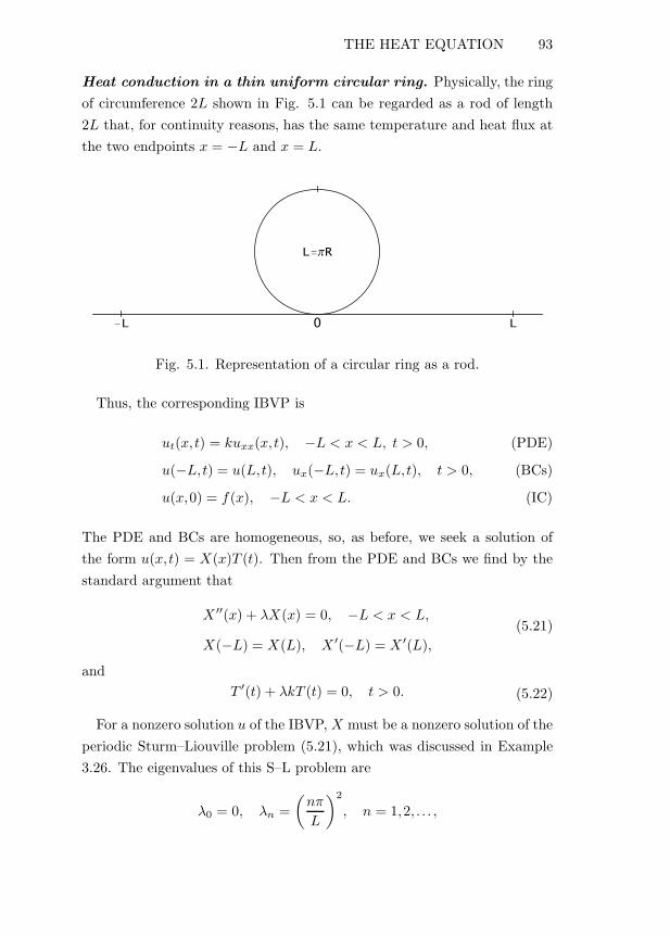
THE HEAT EQUATION 93
Heat conduction in a thin uniform circular ring. Physically, the ringof circumference 2L shown in Fig. 5.1 can be regarded as a rod of length2L that, for continuity reasons, has the same temperature and heat flux atthe two endpoints x = −L and x = L.
0�L L
L�ΠR
Fig. 5.1. Representation of a circular ring as a rod.
Thus, the corresponding IBVP is
ut(x,t) = kuxx(x,t), −L < x < L, t > 0, (PDE)
u(−L,t) = u(L,t), ux(−L,t) = ux(L,t), t > 0, (BCs)
u(x,0) = f(x), −L < x < L. (IC)
The PDE and BCs are homogeneous, so, as before, we seek a solution ofthe form u(x,t) = X(x)T (t). Then from the PDE and BCs we find by thestandard argument that
X ′′(x) + λX(x) = 0, −L < x < L,
X(−L) = X(L), X ′(−L) = X ′(L),(5.21)
andT ′(t) + λkT (t) = 0, t > 0. (5.22)
For a nonzero solution u of the IBVP, X must be a nonzero solution of theperiodic Sturm–Liouville problem (5.21), which was discussed in Example3.26. The eigenvalues of this S–L problem are
λ0 = 0, λn =(nπ
L
)2
, n = 1,2, . . . ,

94 SEPARATION OF VARIABLES
with corresponding eigenfunctions
X0(x) =12, X1n(x) = cos
nπx
L, X2n(x) = sin
nπx
L, n = 1,2, . . . .
Therefore, the time components given by (5.22) with λ = λn are
Tn(t) = Ce−k(nπ/L)2t, C = const,
so we consider a series solution of the form
u(x,t) =12a0 +
∞∑n=1
[anX1n(x) + bnX2n(x)
]Tn(t)
=12a0 +
∞∑n=1
(an cos
nπx
L+ bn sin
nπx
L
)e−k(nπ/L)2t. (5.23)
The IC requires that
u(x,0) = f(x)
=12a0 +
∞∑n=1
(an cos
nπx
L+ bn sin
nπx
L
), −L < x < L.
As mentioned in Example 3.26, the coefficients of this full Fourier series off are computed by means of formulas (2.7)–(2.9):
an =1L
L∫−L
f(x)cosnπx
Ldx, n = 0,1,2, . . . ,
bn =1L
L∫−L
f(x)sinnπx
Ldx, n = 1,2, . . . .
(5.24)
Consequently, the solution of the IBVP is given by (5.23) and (5.24).
5.7. Example. Consider the IBVP
ut(x,t) = uxx(x,t), −1 < x < 1, t > 0,
u(−1, t) = u(1, t), ux(−1, t) = ux(1, t), t > 0,
u(x,0) = x+ 1, −1 < x < 1.

THE WAVE EQUATION 95
Here L = 1 and f(x) = x+ 1, so, by (5.24),
a0 =
1∫−1
(x+ 1)dx = 2,
an =
1∫−1
(x+ 1)cos(nπx)dx = 0,
bn =
1∫−1
(x+ 1)sin(nπx)dx = (−1)n+1 2nπ
.
Hence, by (5.23), the solution of the IBVP is
u(x,t) = 1 +∞∑
n=1
(−1)n+1 2nπ
sin(nπx)e−n2π2t.
5.2. The Wave Equation
Generally speaking, the method of separation of variables is applied toIBVPs for the wave equation in much the same way as for the heat equa-tion. Here, however, the time component satisfies a second-order ODE,which introduces a second IC.
String with fixed endpoints. We know from Section 4.3 that the corre-sponding IBVP is
utt(x,t) = c2uxx(x,t), 0 < x < L, t > 0, (PDE)
u(0, t) = 0, u(L,t) = 0, t > 0, (BCs)
u(x,0) = f(x), ut(x,0) = g(x), 0 < x < L. (ICs)
Since, as in the earlier problems, the PDE and BCs are linear and homoge-neous, we seek a solution of the form
u(x,t) = X(x)T (t),
where, as in the case of the heat equation, neither X nor T can be the zerofunction. Replacing this in the PDE, we obtain
X(x)T ′′(t) = c2X ′′(x)T (t),

96 SEPARATION OF VARIABLES
which, divided by c2X(x)T (t), yields
1c2T ′′(t)T (t)
=X ′′(x)X(x)
= −λ, (5.25)
where λ = const is the separation constant. At the same time, it can beseen that the BCs lead to
X(0) = 0, X(L) = 0;
hence, X satisfies
X ′′(x) + λX(x) = 0, 0 < x < L,
X(0) = 0, X(L) = 0.
This regular S–L problem was solved in Example 3.16, where it was shownthat its eigenvalue-eigenfunction pairs are
λn =(nπ
L
)2
, Xn(x) = sinnπx
L, n = 1,2, . . . . (5.26)
From (5.25) we deduce that for each eigenvalue λn we obtain a functionTn that satisfies the equation
T ′′n (t) + c2λnTn(t) = 0, t > 0,
whose general solution (since λn > 0) is
Tn(t) = b1n cosnπct
L+ b2n sin
nπct
L, b1n, b2n = const. (5.27)
In view of (5.26) and (5.27), we assume that the solution of the IBVP hasthe series representation
u(x,t) =∞∑
n=1
Xn(x)Tn(t)
=∞∑
n=1
sinnπx
L
(b1n cos
nπct
L+ b2n sin
nπct
L
). (5.28)

THE WAVE EQUATION 97
Each term of this series satisfies the PDE and the BCs. To satisfy theICs, we set t = 0 in (5.28) and in the expression of ut(x,t) obtained bydifferentiating (5.28) term by term:
u(x,0) = f(x) =∞∑
n=1
b1n sinnπx
L,
ut(x,0) = g(x) =∞∑
n=1
b2nnπc
Lsin
nπx
L.
We see that the numbers b1n and b2n(nπc)/L are the Fourier sine seriescoefficients of f and g, respectively; so, by (2.10),
b1n =2L
L∫0
f(x)sinnπx
Ldx, n = 1,2, . . . ,
b2n =2nπc
L∫0
g(x)sinnπx
Ldx, n = 1,2, . . . .
(5.29)
Therefore, the solution of the IBVP is given by (5.28) with the b1n and b2n
computed from (5.29).
5.8. Remark. The terms in the expansion of u are called normal modesof vibration. Solutions of this type are called standing waves.
5.9. Example. We notice that in the IBVP
utt(x,t) = uxx(x,t), 0 < x < 1, t > 0,
u(0, t) = 0, u(1, t) = 0, t > 0,
u(x,0) = 3sin(πx) − 2sin(3πx),
ut(x,0) = 4π sin(2πx), 0 < x < 1,
the functions f and g are linear combinations of the eigenfunctions. Settingc = 1 and L = 1 in their eigenfunction expansions above, from Theorem3.20(ii) we deduce that
b11 = 3, b13 = −2, b1n = 0 (n �= 1,3), b22 = 2, b2n = 0 (n �= 2).
Hence, by (5.28), the solution of the IBVP is
u(x,t) = 3sin(πx)cos(πt) − 2sin(3πx)cos(3πt) + 2sin(2πx)sin(2πt).

98 SEPARATION OF VARIABLES
5.10. Example. If the initial conditions in the IBVP in Example 5.9 arereplaced by
u(x,0) ={x, 0 < x ≤ 1/2,1 − x, 1/2 < x < 1,
ut(x,0) = 0, 0 < x < 1,
then, using (5.29) (with c = 1 and L = 1) and integration by parts, we findthat
b1n = 2{ 1/2∫
0
f(x)sin(nπx)dx +
1∫1/2
f(x)sin(nπx)dx}
= 2{ 1/2∫
0
xsin(nπx)dx +
1∫1/2
(1 − x)sin(nπx)dx}
=4
n2π2sin
nπ
2,
b2n =2nπ
1∫0
g(x)sin(nπx)dx = 0, n = 1,2, . . . ;
so, by (5.28), the solution of the IBVP is
u(x,t) =∞∑
n=1
4n2π2
sinnπ
2sin(nπx)cos(nπt).
Vibrating string with free endpoints. The IBVP corresponding to thiscase is (see Section 4.3)
utt(x,t) = c2uxx(x,t), 0 < x < L, t > 0, (PDE)
ux(0, t) = 0, ux(L,t) = 0, t > 0, (BCs)
u(x,0) = f(x), ut(x,0) = g(x), 0 < x < L. (ICs)
Separating the variables, we are led to the eigenvalue-eigenfunction pairs
λn =(nπ
L
)2
, Xn(x) = cosnπx
L, n = 0,1,2, . . . .
For λ0 = 0, the general solution of the equation satisfied by T is
T0(t) =12a10 +
12a20t, a10, a20 = const,

THE WAVE EQUATION 99
while for λn, n ≥ 1, the functions Tn are given by (5.27). Hence, we expectthe solution of the IBVP to be of the form
u(x,t) =12a10 +
12a20t
+∞∑
n=1
cosnπx
L
(a1n cos
nπct
L+ a2n sin
nπct
L
), (5.30)
where the a1n and a2n, n = 0,1,2, . . . , are constants. Every term in (5.30)satisfies the PDE and the BCs.
To satisfy the ICs, we require that
u(x,0) = f(x) =12a10 +
∞∑n=1
a1n cosnπx
L,
ut(x,0) = g(x) =12a20 +
∞∑n=1
a2nnπc
Lcos
nπx
L;
consequently, by (2.11),
a10 =2L
L∫0
f(x)dx,
a1n =2L
L∫0
f(x)cosnπx
Ldx, n = 1,2, . . . ,
a20 =2L
L∫0
g(x)dx,
a2n =2nπc
L∫0
g(x)cosnπx
Ldx, n = 1,2, . . . ,
(5.31)
and we conclude that the solution of the IBVP is given by (5.30) with thea1n and a2n computed by means of (5.31).
5.11. Example. To find the solution of the IBVP
utt(x,t) = uxx(x,t), 0 < x < 1, t > 0,
ux(0, t) = 0, ux(1, t) = 0, t > 0,
u(x,0) = cos(2πx), ut(x,0) = −2π cos(πx), 0 < x < 1,

100 SEPARATION OF VARIABLES
we remark that c = 1 and L = 1, and that the initial data functions f andg are linear combinations of the eigenfunctions; thus,
a12 = 1, a1n = 0 (n �= 2), a21 = −2, a2n = 0 (n �= 1),
so, by (5.30), the solution of the IBVP is
u(x,t) = −2cos(πx)sin(πt) + cos(2πx)cos(2πt).
5.12. Example. Consider the IBVP
utt(x,t) = uxx(x,t), 0 < x < 1, t > 0,
ux(0, t) = 0, ux(1, t) = 0, t > 0,
u(x,0) = 0, ut(x,0) ={−1, 1/4 ≤ x ≤ 3/4,
0 otherwise.
Again, here we have c = 1 and L = 1; so, by (5.31),
a1n = 0, n = 0,1,2, . . . ,
a20 = 2{ 1/4∫
0
g(x)dx +
3/4∫1/4
g(x)dx +
1∫3/4
g(x)dx}
= 2
3/4∫1/4
(−1)dx = −1,
a2n =2nπ
{ 1/4∫0
g(x)cos(nπx)dx +
3/4∫1/4
g(x)cos(nπx)dx
+
1∫3/4
g(x)cos(nπx)dx}
=2nπ
3/4∫1/4
(−1)cos(nπx)dx = − 4n2π2
sinnπ
4cos
nπ
2, n = 1,2, . . . .
Hence, by (5.30), the solution of the IBVP is
u(x,t) = −12t−
∞∑n=1
4n2π2
sinnπ
4cos
nπ
2cos(nπx)sin(nπt).
5.13. Remark. IBVPs with mixed BCs are handled similarly.

THE LAPLACE EQUATION 101
5.3. The Laplace Equation
In this section we discuss the solution of two types of problems: one for-mulated in terms of Cartesian coordinates, and one where the use of polarcoordinates is more appropriate.
The Laplace equation in a rectangle. Consider the equilibrium tem-perature in a uniform rectangle
D = {(x,y) : 0 ≤ x ≤ L, 0 ≤ y ≤ K}, L, K = const}
with no sources and with temperature prescribed on the boundary.The corresponding problem is (see Section 4.2)
uxx(x,y) + uyy(x,y) = 0, 0 < x < L, 0 < y < K,
u(0,y) = f1(y), u(L,y) = f2(y), 0 < y < K,
u(x,0) = g1(x), u(x,K) = g2(x), 0 < x < L.
Although this is a boundary value problem, it turns out that the methodof separation of variables can still be applied. However, since here the BCsare nonhomogeneous, we need to do some additional preliminary work.
By the principle of superposition (see Theorem 1.19), we can seek thesolution of the above BVP as
u(x,y) = u1(x,y) + u2(x,y),
where both u1 and u2 satisfy the PDE, u1 satisfies the BCs with f1(y) = 0,f2(y) = 0, and u2 satisfies the BCs with g1(x) = 0, g2(x) = 0; thus, theBVP for u1 is
(u1)xx(x,y) + (u1)yy(x,y) = 0, 0 < x < L, 0 < y < K, (PDE)
u1(0,y) = 0, u1(L,y) = 0, 0 < y < K,
u1(x,0) = g1(x), u1(x,K) = g2(x), 0 < x < L.(BCs)
We seek a solution of this BVP of the form
u1(x,y) = X(x)Y (y).

102 SEPARATION OF VARIABLES
Clearly, for the same reason as in the case of the heat and wave equations,neither X nor Y can be the zero function. Replacing in the PDE, we obtain
X ′′(x)Y (y) +X(x)Y ′′(y) = 0,
from which, on division by X(x)Y (y), we find that
X ′′(x)X(x)
= −Y′′(y)Y (y)
= −λ,
where λ = const is the separation constant.The two homogeneous BCs yield
X(0)Y (y) = 0, X(L)Y (y) = 0, 0 < y < K.
Since, as already mentioned, Y (y) cannot be identically zero, we concludethat
X(0) = 0, X(L) = 0.
Hence, X is the solution of the regular Sturm–Liouville problem
X ′′(x) + λX(x) = 0, 0 < x < L,
X(0) = 0, X(L) = 0.
From Example 3.16 we know that the eigenvalue-eigenfunction pairs ofthis problem are
λn =(nπ
L
)2
, Xn(x) = sinnπx
L, n = 1,2, . . . . (5.32)
Then for each n = 1,2, . . . we seek functions Yn that satisfy
Y ′′n (y) −
(nπ
L
)2
Yn(y) = 0, 0 < y < K.
By Remark 1.4, the general solution of the equation for Yn can be writtenas
Yn(y) = C1n sinhnπ(y −K)
L+ C2n sinh
nπy
L, C1n, C2n = const. (5.33)

THE LAPLACE EQUATION 103
In view of (5.32) and (5.33), it seems reasonable to expect u1 to be of theform
u1(x,y) =∞∑
n=1
Xn(x)Yn(y)
=∞∑
n=1
sinnπx
L
(C1n sinh
nπ(y −K)L
+ C2n sinhnπy
L
), (5.34)
where each term satisfies the PDE and the two homogeneous BCs. Tosatisfy the two remaining, nonhomogeneous BCs, we must have
u1(x,0) = g1(x)
=∞∑
n=1
(− C1n sinh
nπK
L
)sin
nπx
L=
∞∑n=1
b1n sinnπx
L,
u1(x,K) = g2(x)
=∞∑
n=1
(C2n sinh
nπK
L
)sin
nπx
L=
∞∑n=1
b2n sinnπx
L;
in other words, we need the Fourier sine series of g1 and g2. By (2.10), forn = 1,2, . . . ,
b1n = −C1n sinhnπK
L=
2L
L∫0
g1(x)sinnπx
Ldx,
b2n = C2n sinhnπK
L=
2L
L∫0
g2(x)sinnπx
Ldx;
therefore,
C1n = − b1n
sinh(nπK/L)= − 2
Lcsch(nπK/L)
L∫0
g1(x)sinnπx
Ldx, (5.35)
C2n =b2n
sinh(nπK/L)=
2L
csch(nπK/L)
L∫0
g2(x)sinnπx
Ldx. (5.36)
This means that the function u1(x,y) is given by (5.34) with the coefficientsC1n and C2n computed from (5.35) and (5.36).
The procedure for finding u2 is similar, with the obvious modifications.
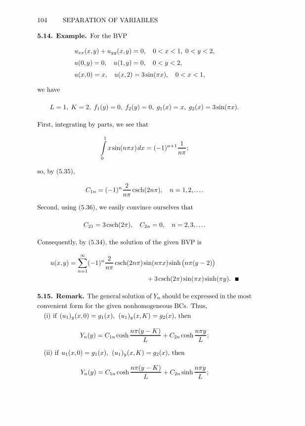
104 SEPARATION OF VARIABLES
5.14. Example. For the BVP
uxx(x,y) + uyy(x,y) = 0, 0 < x < 1, 0 < y < 2,
u(0,y) = 0, u(1,y) = 0, 0 < y < 2,
u(x,0) = x, u(x,2) = 3sin(πx), 0 < x < 1,
we have
L = 1, K = 2, f1(y) = 0, f2(y) = 0, g1(x) = x, g2(x) = 3sin(πx).
First, integrating by parts, we see that
1∫0
xsin(nπx)dx = (−1)n+1 1nπ
;
so, by (5.35),
C1n = (−1)n 2nπ
csch(2nπ), n = 1,2, . . . .
Second, using (5.36), we easily convince ourselves that
C21 = 3csch(2π), C2n = 0, n = 2,3, . . . .
Consequently, by (5.34), the solution of the given BVP is
u(x,y) =∞∑
n=1
(−1)n 2nπ
csch(2nπ)sin(nπx)sinh(nπ(y − 2)
)+ 3csch(2π)sin(πx)sinh(πy).
5.15. Remark. The general solution of Yn should be expressed in the mostconvenient form for the given nonhomogeneous BCs. Thus,
(i) if (u1)y(x,0) = g1(x), (u1)y(x,K) = g2(x), then
Yn(y) = C1n coshnπ(y −K)
L+ C2n cosh
nπy
L;
(ii) if u1(x,0) = g1(x), (u1)y(x,K) = g2(x), then
Yn(y) = C1n coshnπ(y −K)
L+ C2n sinh
nπy
L;
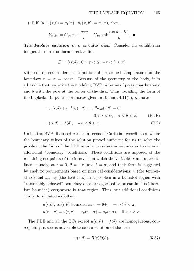
THE LAPLACE EQUATION 105
(iii) if (u1)y(x,0) = g1(x), u1(x,K) = g2(x), then
Yn(y) = C1n coshnπy
L+ C2n sinh
nπ(y −K)L
.
The Laplace equation in a circular disk. Consider the equilibriumtemperature in a uniform circular disk
D = {(r,θ) : 0 ≤ r < α, −π < θ ≤ π}
with no sources, under the condition of prescribed temperature on theboundary r = α = const. Because of the geometry of the body, it isadvisable that we write the modeling BVP in terms of polar coordinates rand θ with the pole at the center of the disk. Thus, recalling the form ofthe Laplacian in polar coordinates given in Remark 4.11(ii), we have
urr(r,θ) + r−1ur(r,θ) + r−2uθθ(r,θ) = 0,
0 < r < α, −π < θ < π, (PDE)
u(α,θ) = f(θ), −π < θ ≤ π. (BC)
Unlike the BVP discussed earlier in terms of Cartesian coordinates, wherethe boundary values of the solution proved sufficient for us to solve theproblem, the form of the PDE in polar coordinates requires us to consideradditional “boundary” conditions. These conditions are imposed at theremaining endpoints of the intervals on which the variables r and θ are de-fined, namely, at r = 0, θ = −π, and θ = π, and their form is suggestedby analytic requirements based on physical considerations: u (the temper-ature) and ur, uθ (the heat flux) in a problem in a bounded region with“reasonably behaved” boundary data are expected to be continuous (there-fore bounded) everywhere in that region. Thus, our additional conditionscan be formulated as follows:
u(r,θ), ur(r,θ) bounded as r → 0+, −π < θ < π,
u(r,−π) = u(r,π), uθ(r,−π) = uθ(r,π), 0 < r < α.
The PDE and all the BCs except u(α,θ) = f(θ) are homogeneous; con-sequently, it seems advisable to seek a solution of the form
u(r,θ) = R(r)Θ(θ). (5.37)

106 SEPARATION OF VARIABLES
Then the last two (periodic) BCs become
Θ(−π)R(r) = Θ(π)R(r), Θ′(−π)R(r) = Θ′(π)R(r), 0 < r < α,
from which, to avoid the identically zero—hence, unacceptable—solution,we deduce that
Θ(−π) = Θ(π), Θ′(−π) = Θ′(π).
In view of (5.37), the PDE can be written as
[R′′(r) + r−1R′(r)
]Θ(θ) + r−2R(r)Θ′′(θ) = 0,
which, on division by r−2R(r)Θ(θ) and in accordance with the usual argu-ment, yields
Θ′′(θ)Θ(θ)
= −r2R′′(r) + rR′(r)
R(r)= −λ, (5.38)
where λ = const is the separation constant. Then Θ is a solution of theperiodic Sturm–Liouville problem
Θ′′(θ) + λΘ(θ) = 0, −π < θ < π,
Θ(−π) = Θ(π), Θ′(−π) = Θ′(π).
This problem was discussed in Example 3.26. Hence, for L = π, the eigen-values and their corresponding eigenfunctions are, respectively,
λ0 = 0, λn = n2, n = 1,2, . . . ,
Θ0(θ) = 1, Θ1n(θ) = cos(nθ), Θ2n(θ) = sin(nθ), n = 1,2, . . . .
From the second equality in (5.38) we see that for each n = 0,1,2, . . . thecorrespondent radial component Rn satisfies
r2R′′n(r) + rR′
n(r) − n2Rn = 0, 0 < r < α. (5.39)
This is a Cauchy–Euler equation, for which, if n �= 0, we seek solutions ofthe form (see Section 1.4)
Rn(r) = rp, p = const.

THE LAPLACE EQUATION 107
Replacing in (5.39), we find that
[p(p− 1) + p− n2]rp = 0,
or p2 − n2 = 0, with roots p1 = n and p2 = −n. Therefore, the generalsolution of (5.39) in this case is
Rn(r) = C1rn + C2r
−n, C1, C2 = const. (5.40)
If n = 0, then (5.39) reduces to (rR′0(r))
′ = 0, so
rR′0(r) = C2 = const;
in turn, this leads to R′0(r) = r−1C2 and then to the general solution
R0(r) = C1 + C2 lnr, C1, C2 = const. (5.41)
From (5.37) and the condition of boundedness at r = 0 we deduce thatall the numbers Rn(0) must be finite. As (5.40) and (5.41) indicate, thishappens only if C2 = 0 and C2 = 0; in other words,
R0(r) = C1, Rn(r) = C1rn, n = 1,2, . . . .
Taking the arbitrary constant equal to 1, we express this by the singleformula
Rn(r) = rn, n = 0,1,2, . . . .
In accordance with the separation of variables procedure, we expect thesolution of the IBVP to have a series representation of the form
u(r,θ) =12a0R0(r)Θ0(θ) +
∞∑n=1
Rn(r)[anΘ1n(θ) + bnΘ2n(θ)
]
=12a0 +
∞∑n=1
rn[an cos(nθ) + bn sin(nθ)
], (5.42)
where each term satisfies the PDE and the three homogeneous BCs. Theunknown numerical coefficients 1
2 a0, an, and bn are determined from the

108 SEPARATION OF VARIABLES
remaining (nonhomogeneous) condition:
u(α,θ) = f(θ) = 12 a0 +
∞∑n=1
αn[an cos(nθ) + bn sin(nθ)
],
− π < θ ≤ π. (5.43)
This is the full Fourier series for f with L = π and coefficients 12 a0, αnan,
and αnbn; so, by (2.7)–(2.9),
a0 =1π
π∫−π
f(θ)dθ,
an =1παn
π∫−π
f(θ)cos(nθ)dθ, n = 1,2, . . . , (5.44)
bn =1παn
π∫−π
f(θ)sin(nθ)dθ, n = 1,2, . . . .
Consequently, the solution of the BVP is given by (5.42) with the a0, an,and bn computed by means of (5.44).
5.16. Remark. From (5.42) and (5.44) it follows that
u(0,θ) =12a0 =
12π
π∫−π
f(θ)dθ;
in other words, the temperature at the center of the disk is equal to theaverage of the temperature on the boundary circle. This result, alreadyused in the proof of Theorem 4.14, is called the mean value property for theLaplace equation.
5.17. Example. In the BVP
(Δu)(r,θ) = 0, 0 < r < 2, −π < θ < π,
u(2,θ) = 1 + 8sinθ − 32cos(4θ), −π < θ < π,
we haveα = 2, f(θ) = 1 + 8sinθ − 32cos(4θ).

OTHER EQUATIONS 109
Since f is a linear combination of the eigenfunctions associated with thisproblem, we use (5.43) and Theorem 3.20(ii) to deduce that 1
2 a0 = 1,24a4 = −32, and 2b1 = 8, while the remaining coefficients are zero; there-fore,
a0 = 2, a4 = −2, an = 0 (n �= 0,4), b1 = 4, bn = 0 (n �= 1),
which means that, by (5.42), the solution of the given BVP is
u(r,θ) = 1 + 4r sinθ − 2r4 cos(4θ).
5.4. Other Equations
The method of separation of variables can also be applied to problems in-volving some of the equations mentioned in Section 4.4.
5.18. Example. Consider the diffusion–convection IBVP
ut(x,t) = 2uxx(x,t) − ux(x,t), 0 < x < 1, t > 0, (PDE)
u(0, t) = 0, u(1, t) = 0, t > 0, (BCs)
u(x,0) = −2ex/4 sin(3πx), 0 < x < 1. (IC)
Applying the arguments developed earlier in this chapter, we seek the so-lution in the form u(x,t) = X(x)T (t) and, from the PDE and BCs, deducethat the components X and T satisfy
2X ′′(x) −X ′(x) + λX(x) = 0, 0 < x < 1,
X(0) = 0, X(1) = 0, t > 0,(5.45)
andT ′(t) + λT (t) = 0, t > 0. (5.46)
The regular Sturm–Liouville problem (5.45) is solved by the method usedin Example 3.19, and its eigenvalues and eigenfunctions are found to be
λn = 18 (16n2π2 + 1), Xn(x) = ex/4 sin(nπx), n = 1,2, . . . .
Then (5.46) becomes
Tn(t) + 18 (16n2π2 + 1)Tn(t) = 0,

110 SEPARATION OF VARIABLES
with general solution
Tn(t) = cne−(16n2π2+1)t/8, cn = const.
Combining the Xn and Tn in the usual way, we find that the function
u(x,t) =∞∑
n=1
cnex/4−(16n2π2+1)t/8 sin(nπx) (5.47)
satisfies both the PDE and the BCs.The coefficients cn are found from the IC; thus, for t = 0 we must have
u(x,0) =∞∑
n=1
cnex/4 sin(nπx) = −2ex/4 sin(3πx),
from which
c3 = −2, cn = 0 (n �= 3),
so the solution, given by (5.47), of the IBVP is
u(x,t) = −2ex/4−(144π2+1)t/8 sin(3πx).
5.19. Example. Consider the dissipative wave propagation problem
utt(x,t) + 2ut(x,t) = uxx(x,t) − 3ux(x,t),
0 < x < 1, t > 0,
u(0, t) = 0, u(1, t) = 0, t > 0,
u(x,0) = −e3x/2 sin(2πx), ut(x,0) = 2e3x/2 sin(πx),
0 < x < 1.
Writing u(x,t) = X(x)T (t) and proceeding as in Example 5.18, we findthat
X ′′(x) − 3X ′(x) + λX(x) = 0, 0 < x < 1,
X(0) = 0, X(1) = 0,(5.48)
and
T ′′(t) + 2T ′ + λT (t) = 0. (5.49)
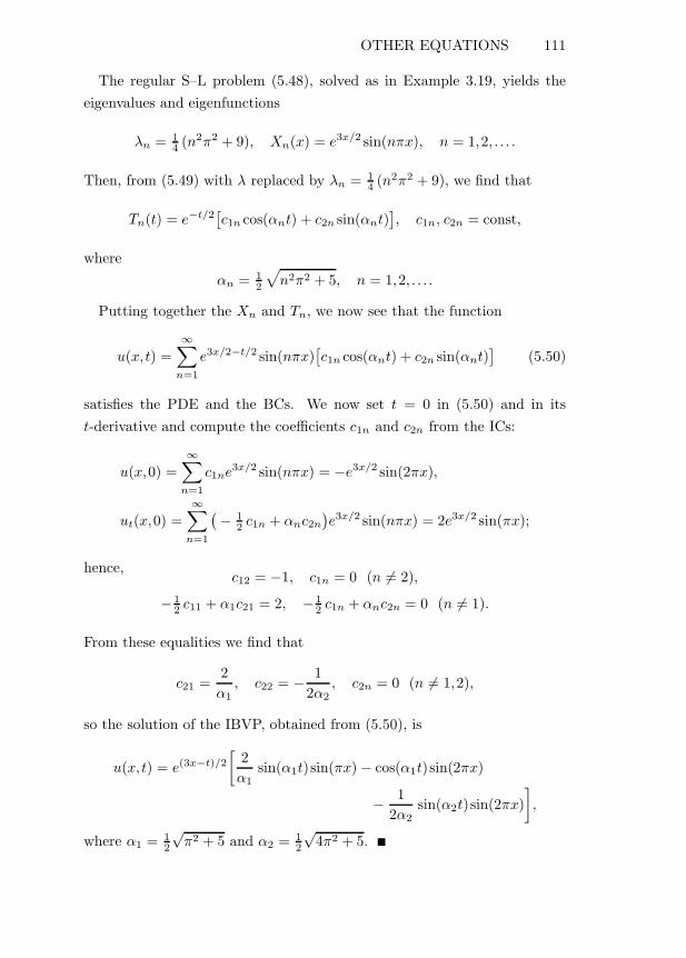
OTHER EQUATIONS 111
The regular S–L problem (5.48), solved as in Example 3.19, yields theeigenvalues and eigenfunctions
λn = 14 (n2π2 + 9), Xn(x) = e3x/2 sin(nπx), n = 1,2, . . . .
Then, from (5.49) with λ replaced by λn = 14 (n2π2 + 9), we find that
Tn(t) = e−t/2[c1n cos(αnt) + c2n sin(αnt)
], c1n, c2n = const,
whereαn = 1
2
√n2π2 + 5, n = 1,2, . . . .
Putting together the Xn and Tn, we now see that the function
u(x,t) =∞∑
n=1
e3x/2−t/2 sin(nπx)[c1n cos(αnt) + c2n sin(αnt)
](5.50)
satisfies the PDE and the BCs. We now set t = 0 in (5.50) and in itst-derivative and compute the coefficients c1n and c2n from the ICs:
u(x,0) =∞∑
n=1
c1ne3x/2 sin(nπx) = −e3x/2 sin(2πx),
ut(x,0) =∞∑
n=1
( − 12 c1n + αnc2n
)e3x/2 sin(nπx) = 2e3x/2 sin(πx);
hence,c12 = −1, c1n = 0 (n �= 2),
− 12 c11 + α1c21 = 2, − 1
2 c1n + αnc2n = 0 (n �= 1).
From these equalities we find that
c21 =2α1, c22 = − 1
2α2, c2n = 0 (n �= 1,2),
so the solution of the IBVP, obtained from (5.50), is
u(x,t) = e(3x−t)/2
[2α1
sin(α1t)sin(πx) − cos(α1t)sin(2πx)
− 12α2
sin(α2t)sin(2πx)],
where α1 = 12
√π2 + 5 and α2 = 1
2
√4π2 + 5.

112 SEPARATION OF VARIABLES
5.20. Example. Consider the two-dimensional steady state diffusion–con-vection problem
uxx(x,y) + uyy(x,y) − 2ux(x,y) = 0, 0 < x < 1, 0 < y < 2, (PDE)
u(0,y) = 0, u(1,y) = −3sin(πy), 0 < y < 2,
u(x,0) = 0, u(x,2) = 0, 0 < x < 1.(BCs)
Seeking the solution in the form u(x,y) = X(x)Y (y), from the PDE andthe last two (homogeneous) BCs it follows that
X ′′(x) − 2X ′(x) − λX(x) = 0, 0 < x < 1, (5.51)
andY ′′(y) + λY (y) = 0, 0 < y < 2,
Y (0) = 0, Y (1) = 0.
The regular S–L problem for Y has been solved in Example 3.16 and hasthe eigenvalues and eigenfunctions
λn =n2π2
4, Yn(y) = sin
nπy
2, n = 1,2, . . . ,
so (5.51) becomes
X ′′n(x) − 2X ′
n(x) − n2π2
4Xn(x) = 0,
with general solution
Xn(x) = c1nes1nx + c2ne
s2nx,
where
s1n = 1 + 12
√n2π2 + 4, s2n = 1 − 1
2
√n2π2 + 4, c1n, c2n = const.
Consequently, the function
u(x,y) =∞∑
n=1
sinnπy
2(c1ne
s1nx + c2nes2nx
)(5.52)
satisfies the PDE and the last two BCs. The coefficients c1n and c2n aredetermined from the first two BCs; thus, setting x = 0 and then x = 1 in(5.52), we find that

EQUATIONS WITH MORE THAN TWO VARIABLES 113
∞∑n=1
(c1n + c2n)sinnπy
2= 0,
∞∑n=1
(c1ne
s1n + c2nes2n
)sin
nπy
2= −3sin(πy),
so
c1n + c2n = 0, n = 1,2, . . . ,
c12es12 + c22e
s22 = −3, c1nes1n + c2ne
s2n = 0 (n �= 2).
Then
c12 = −c22 =3
es22 − es12, c1n = c2n = 0 (n �= 2),
which, substituted in (5.52), yield the solution of the given BVP:
u(x,y) =3
es22 − es12
(es12x − es22x
)sin(πy),
where
s12 = 1 +√π2 + 1, s22 = 1 −
√π2 + 1.
5.5. Equations with More than Two Variables
In Section 4.2 we derived a model for heat conduction in a uniform plate,where the unknown temperature function depends on the time variable andtwo space variables. Here we consider the two-dimensional analog of thewave equation and solve it by the method of separation of variables interms of both Cartesian and polar coordinates.
Vibrating rectangular membrane. A vibrating rectangular membranewith negligible body force and clamped edges is modeled by the IBVP
utt(x,t) = c2(Δu)(x,y) = c2[uxx(x,y) + uyy(x,y)
],
0 < x < L, 0 < y < K, t > 0, (PDE)
u(0,y, t) = 0, u(L,y,t) = 0, 0 < y < K, t > 0,
u(x,0, t) = 0, u(x,K,t) = 0, 0 < x < L, t > 0,(BCs)
u(x,y,0) = f(x,y), ut(x,y,0) = g(x,y),
0 < x < L, 0 < y < K. (ICs)

114 SEPARATION OF VARIABLES
Since the PDE and BCs are linear and homogeneous, we seek the solutionas a product of a function of the space variables and a function of the timevariable:
u(x,y,t) = S(x,y)T (t). (5.53)
Reasoning as in previous similar situations, from the PDE and BCs we findthat T satisfies the ODE
T ′′(t) + λc2T (t) = 0, t > 0,
and that S is a solution of the BVP
Sxx(x,y) + Syy(x,y) + λS(x,y) = 0,
0 < x < L, 0 < y < K,
S(0,y) = 0, S(L,y) = 0, 0 < y < K,
S(x,0) = 0, S(x,K) = 0, 0 < x < L,
(5.54)
where λ = const is the separation constant.We notice that the PDE and BCs for S are themselves linear and homo-
geneous, so we use separation of variables once more and seek a solution for(5.54) of the form
S(x,y) = X(x)Y (y). (5.55)
The PDE in (5.54) then becomes
X ′′(x)Y (y) +X(x)Y ′′(y) = −λX(x)Y (y),
which, on division by X(x)Y (y), yields
X ′′(x)X(x)
= −λ− Y ′′(y)Y (y)
= −μ,
where μ = const is a second separation constant.From the above chain of equalities and the BCs in (5.54) we find in the
usual way that X and Y are, respectively, solutions of the regular Sturm–Liouville problems
X ′′(x) + μX(x) = 0, 0 < x < L,
X(0) = 0, X(L) = 0,(5.56)

EQUATIONS WITH MORE THAN TWO VARIABLES 115
andY ′′(y) + (λ− μ)Y (y) = 0, 0 < y < K,
Y (0) = 0, Y (K) = 0.(5.57)
The nonzero solutions that we require for (5.56) are the eigenfunctions ofthis S–L problem, which were computed in Example 3.16 together with thecorresponding eigenvalues:
μn =(nπ
L
)2
, Xn(x) = sinnπx
L, n = 1,2, . . . .
For each fixed value of n, the function Y satisfies the S–L problem (5.57)with μ = μn. Since this problem is similar to (5.56), its eigenvalues andeigenfunctions (nonzero solutions) are
λnm − μn =(mπ
K
)2
, Ynm(y) = sinmπy
K, m = 1,2, . . . .
We remark that (5.54) may be regarded as a two-dimensional eigenvalueproblem with eigenvalues
λnm = μn +(mπ
K
)2
=(nπ
L
)2
+(mπ
K
)2
, n, m = 1,2, . . . ,
and corresponding eigenfunctions
Snm(x,y) = Xn(x)Ynm(y) = sinnπx
Lsin
mπy
K, n, m = 1,2, . . . .
Going back to the equation satisfied by T , for λ = λnm we obtain thefunctions
Tnm(t) = anm cos(√
λnm ct)
+ bnm sin(√
λnm ct), anm, bnm = const.
From this, (5.53), and (5.55) we now conclude that the solution of theoriginal IBVP should have a representation of the form
u(x,y,t) =∞∑
n=1
∞∑m=1
Snm(x,y)Tnm(t)
=∞∑
n=1
∞∑m=1
sinnπx
Lsin
mπy
K
× [anm cos
(√λnm ct
)+ bnm sin
(√λnm ct
)]. (5.58)
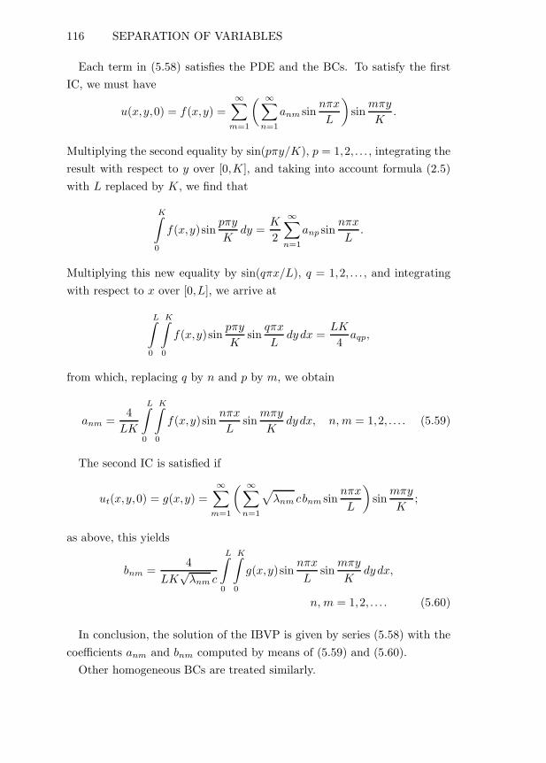
116 SEPARATION OF VARIABLES
Each term in (5.58) satisfies the PDE and the BCs. To satisfy the firstIC, we must have
u(x,y,0) = f(x,y) =∞∑
m=1
( ∞∑n=1
anm sinnπx
L
)sin
mπy
K.
Multiplying the second equality by sin(pπy/K), p = 1,2, . . . , integrating theresult with respect to y over [0,K], and taking into account formula (2.5)with L replaced by K, we find that
K∫0
f(x,y)sinpπy
Kdy =
K
2
∞∑n=1
anp sinnπx
L.
Multiplying this new equality by sin(qπx/L), q = 1,2, . . . , and integratingwith respect to x over [0,L], we arrive at
L∫0
K∫0
f(x,y)sinpπy
Ksin
qπx
Ldydx =
LK
4aqp,
from which, replacing q by n and p by m, we obtain
anm =4LK
L∫0
K∫0
f(x,y)sinnπx
Lsin
mπy
Kdydx, n, m = 1,2, . . . . (5.59)
The second IC is satisfied if
ut(x,y,0) = g(x,y) =∞∑
m=1
( ∞∑n=1
√λnm cbnm sin
nπx
L
)sin
mπy
K;
as above, this yields
bnm =4
LK√λnm c
L∫0
K∫0
g(x,y)sinnπx
Lsin
mπy
Kdydx,
n, m = 1,2, . . . . (5.60)
In conclusion, the solution of the IBVP is given by series (5.58) with thecoefficients anm and bnm computed by means of (5.59) and (5.60).
Other homogeneous BCs are treated similarly.

EQUATIONS WITH MORE THAN TWO VARIABLES 117
5.21. Example. In the IBVP
utt(x,y,t) = uxx(x,y,t) + uyy(x,y,t),
0 < x < 1, 0 < y < 2, t > 0,
u(0,y, t) = 0, u(1,y, t) = 0, 0 < y < 2, t > 0,
u(x,0, t) = 0, u(x,2, t) = 0, 0 < x < 1, t > 0,
u(x,y,0) = sin(2πx)[sin(1
2πy) − 2sin(πy)],
0 < x < 1, 0 < y < 2,
ut(x,y,0) = 2sin(2πx)sin(12πy), 0 < x < 1, 0 < y < 2,
we have c = 1, L = 1, and K = 2; thus, comparing the initial data functionswith the double Fourier series expansions of f and g, we see that
a21 = 1, a22 = −2, a2m = 0 (m �= 1,2),√λ21 b21 = 2,
√λ2m b2m = 0 (m �= 1).
Since λ21 = (2π)2 + (π/2)2 = 17π2/4, formula (5.58) yields the solution
u(x,y,t) = sin(2πx)sin(
12πy
)cos
(12
√17πt
)− 2sin(2πx)sin(πy)cos
(√5πt
)+
(4π/
√17
)sin(2πx)sin
(12πy
)sin
(12
√17πt
).
Vibrating circular membrane. A two-dimensional body of this type isdefined in polar coordinates by 0 ≤ r ≤ α, −π < θ ≤ π. If the body forceis negligible and the boundary r = α is clamped (fixed), then the verticalvibrations of the membrane are described by the IBVP
utt(r,θ, t) = c2(Δu)(r,θ, t), 0 < r < α, −π < θ < π, t > 0, (PDE)
u(α,θ,t) = 0, u(r,θ, t), ur(r,θ, t) bounded as r → 0+,
− π < θ < π, t > 0,
u(r,−π,t) = u(r,π,t), uθ(r,−π,t) = uθ(r,π,t),
0 < r < α, t > 0,(BCs)
u(r,θ,0) = f(r,θ), ut(r,θ,0) = g(r,θ),
0 < r < α, −π < θ < π. (ICs)

118 SEPARATION OF VARIABLES
As in Section 5.3, the BCs at r = 0 and θ = −π, π express the continuity(therefore boundedness) of the displacement (u) and tension (ur, uθ) in themembrane for “reasonably behaved” functions f and g.
Since the PDE and BCs are linear and homogeneous, we try the methodof separation of variables and seek a solution of the form
u(r,θ, t) = S(r,θ)T (t). (5.61)
Then, following the standard procedure, from the PDE and BCs we findthat S is a solution of the problem
(ΔS)(r,θ) + λS(r,θ) = 0, 0 < r < α, −π < θ < π,
S(α,θ) = 0, S(r,θ), Sr(r,θ) bounded as r → 0+, −π < θ < π,
S(r,−π) = S(r,π), Sθ(r,−π) = Sθ(r,π), 0 < r < α,
(5.62)
where λ = const is the separation constant, while T satisfies
T ′′(t) + λc2T (t) = 0, t > 0.
Since the PDE and BCs for S are linear and homogeneous, we seek S ofthe form
S(r,θ) = R(r)Θ(θ). (5.63)
Next, recalling the expression of the Laplacian in polar coordinates (seeRemark 4.11(ii)), we write the PDE in (5.62) as
[R′′(r) + r−1R′(r)
]Θ(θ) + r−2R(r)Θ′′(θ) + λR(r)Θ(θ) = 0,
which, on division by r−2R(r)Θ(θ), yields
Θ′′(θ)Θ(θ)
= −r2R′′(r) + rR′(r)
R(r)− λr2 = −μ,
where μ = const is a second separation constant.Applying the usual argument to the BCs, we now conclude that R and
Θ are solutions of Sturm–Liouville problems. First, Θ satisfies the periodicS–L problem
Θ′′(θ) + μΘ(θ) = 0, −π < θ < π,
Θ(−π) = Θ(π), Θ′(−π) = Θ′(π),

EQUATIONS WITH MORE THAN TWO VARIABLES 119
whose eigenvalues and eigenfunctions, computed in Example 3.26, are
μ0 = 0, Θ0(θ) = 12 ,
μn = n2, Θ1n(θ) = cos(nθ), Θ2n(θ) = sin(nθ), n = 1,2, . . . .
For each fixed value of n, we compute a solution Rn of the singular S–Lproblem
r2R′′n(r) + rR′
n(r) + (λr2 − n2)Rn(r) = 0, 0 < r < α,
Rn(α) = 0, Rn(r), R′n(r) bounded as r → 0+.
This is the singular Sturm–Liouville problem (3.12), (3.13) (with m re-placed by n) discussed in Section 3.3, which has countably many eigenvaluesand a complete set of corresponding eigenfunctions
λnm =(ξnm
α
)2
, Rnm(r) = Jn
(ξnmr
α
), n = 0,1,2, . . . , m = 1,2, . . . ,
where Jn is the Bessel function of the first kind and order n and ξnm arethe zeros of Jn.
Returning to the ODE satisfied by T , for λ = λnm = (ξnm/α)2 we nowobtain the solutions
Tnm(t) = Anm cosξnmct
α+Bnm sin
ξnmct
α, Anm, Bnm = const.
Suppose, for simplicity, that g = 0; then it is clear that the sine term inTnm must vanish. Hence, if we piece together the various components of uaccording to (5.61) and (5.63), we conclude that the solution of the IBVPshould be of the form
u(r,θ, t) =∞∑
n=0
∞∑m=1
[anmΘ1n(θ) + bnmΘ2n(θ)
]Rnm(r)Tnm(t)
=∞∑
n=0
∞∑m=1
[anm cos(nθ) + bnm sin(nθ)
]Jn
(ξnmr
α
)cos
ξnm ct
α.
Each term in this sum satisfies the PDE, the BCs, and the second IC. Tosatisfy the first IC, we need to have
u(r,θ,0) = f(r,θ) =∞∑
m=1
{ ∞∑n=0
[anm cos(nθ) + bnm sin(nθ)
]}Jn
(ξnmr
α
).

120 SEPARATION OF VARIABLES
The anm and bnm are now computed as in other problems of this type, bymeans of the orthogonality properties of cos(nθ), sin(nθ), and Jn(ξnmr/α)expressed by (2.4)–(2.6) with L = π and by (3.16).
5.22. Remark. In the circularly symmetric case (that is, when the datafunctions are independent of θ) we use the solution split u(r,t) = R(r)T (t).Here the problem reduces to solving Bessel’s equation of order zero. In theend, we obtain
u(r,t) =∞∑
m=1
[am cos
(√λm ct
)+ bm sin
(√λm ct
)]J0
(√λm r
),
where λm is the same as λ0m = (ξ0m/α)2 in the general problem and theam and bm are determined from the property of orthogonality with weightr on [0,α] of the functions J0
(√λm r
).
5.23. Example. With α = 1, c = 1, f(r,θ) = 1, and g(r,θ) = 0, theformula in Remark 5.22 yields
u(r,0) =∞∑
m=1
amJ0
(√λm r
)= 1,
ut(r,0) =∞∑
m=1
bm√λmJ0
(√λm r
)= 0,
so the am are the coefficients of the expansion of the constant function 1 inthe functions J0
(√λm r
)on (0,1) and bm = 0. Since, with a computational
approximation to four decimal places,
1 = 1.6020J0(2.4048r) − 1.0463J0(5.5201r) + 0.8514J0(8.6537r) + · · · ,
it follows that
a1 = 1.6020, a2 = −1.0463, a3 = 0.8514, . . . ,
so the solution of the problem is
u(r,t) = 1.6020cos(2.4048t)J0(2.4048r)
− 1.0463cos(5.5201t)J0(5.5201r)
+ 0.8514cos(8.6537t)J0(8.6537r) + · · · .
EQUATIONS WITH MORE THAN TWO VARIABLES 121
Equilibrium temperature in a solid sphere. The steady state distri-bution of heat inside a homogeneous sphere of radius α when the (time-independent) temperature is prescribed on the surface and no sources arepresent is the solution of the BVP
Δu(r,θ,ϕ) = 0, 0 < r < α, 0 < θ < 2π, 0 < ϕ < π, (PDE)
u(α,θ,ϕ) = f(θ,ϕ), u(r,θ,ϕ), ur(r,θ,ϕ) bounded as r → 0+,
0 < θ < 2π, 0 < ϕ < π,
u(r,0,ϕ) = u(r,2π,ϕ), uθ(r,0,ϕ) = uθ(r,2π,ϕ),
0 < r < α, 0 < ϕ < π,(BCs)
u(r,θ,ϕ), uϕ(r,θ,ϕ) bounded as ϕ→ 0+ and as ϕ→ π−,0 < r < α, 0 < θ < 2π,
where f is a known function. The first boundary condition represents thegiven surface temperature; the remaining ones have been adjoined on thebasis of arguments similar to those used in the case of a uniform circulardisk.
In terms of the spherical coordinates r, θ, ϕ, the above PDE is written as(see Remark 4.11(v))
1r2
(r2ur)r +1
r2 sin2ϕuθθ +
1r2 sinϕ
((sinϕ)uϕ)ϕ = 0.
Since the PDE and all but one of the BCs are homogeneous, we try asolution of the form
u(r,θ,ϕ) = R(r)Θ(θ)Φ(ϕ).
As before, the nonhomogeneous BC implies that none of R,Θ,Φ can bethe zero function. Replacing in the PDE and multiplying every term by(r2 sin2ϕ)/(RΘΦ), we find that
Θ′′
Θ= −(sin2ϕ)
(r2R′)′
R− (sinϕ)
((sinϕ)Φ′)′
Φ,
where the left-hand side is a function of θ and the right-hand side is afunction of r and ϕ. Consequently, both sides must be equal to one and thesame constant, which, for convenience, we denote by −μ. This leads to thepair of equations
122 SEPARATION OF VARIABLES
Θ′′(θ) + μΘ(θ) = 0, 0 < θ < 2π, (5.64)
(r2R′)′
R+
1sinϕ
((sinϕ)Φ′)′
Φ− μ
sin2ϕ= 0,
0 < r < α, 0 < ϕ < π. (5.65)
(In (5.65) we have also divided by sin2ϕ.)To avoid the identically zero solution, from the two periodicity conditions
in the BVP we deduce in the usual way that
Θ(0) = Θ(2π), Θθ(0) = Θθ(2π). (5.66)
The regular S–L problem (5.64), (5.66) for Θ is the same as in the case ofthe circular membrane; it has the eigenvalues μ = m2, m = 0,1,2, . . . , andcorresponding eigenfunctions
Θm(θ) = C1m cos(mθ) + C2m sin(mθ),
which, using Euler’s formula, we can rewrite as
Θm(θ) = C′1me
imθ + C′12e
−imθ. (5.67)
We now operate a second separation of variables, this time in (5.65):
1sinϕ
((sinϕ)Φ′)′
Φ− m2
sin2ϕ=
(r2R′)′
R= −λ = const;
this yields the equations
1sinϕ
((sinϕ)Φ′(ϕ)
)′ +(λ− m2
sin2ϕ
)Φ(ϕ) = 0, 0 < ϕ < π, (5.68)
(r2R′)′ − λR = 0, 0 < r < α. (5.69)
In (5.68) we substitute
ξ = cosϕ, dξ = −sinϕdϕ,d
dξ= − 1
sinϕd
dϕ,
sin2ϕ = 1 − cos2ϕ = 1 − ξ2, Φ(ϕ) = Ψ(ξ)
and bring the equation to the form
((1 − ξ2)Ψ′(ξ)
)′ +(λ− m2
1 − ξ2
)Ψ(ξ) = 0, −1 < ξ < 1. (5.70)
EQUATIONS WITH MORE THAN TWO VARIABLES 123
The boundary conditions for Ψ are obtained from those at ϕ = 0 and ϕ = π
in the original problem by recalling that Φ cannot be the zero function:
Ψ(ξ), Ψ′(ξ) bounded as ξ → −1+ and as ξ → 1−. (5.71)
We remark that (5.70), (5.71) is the singular S–L problem for the asso-ciated Legendre equation mentioned in Section 3.5, with eigenvalues andeigenfunctions
λn = n(n+ 1), Ψ(ξ) = Pmn (ξ), n = m,m+ 1, . . . ,
where Pmn are the associated Legendre functions; consequently,
Φn(ϕ) = Pmn (cosϕ). (5.72)
Turning to the Cauchy–Euler equation (5.69) with λ = n(n+ 1), we findthat its general solution (see Section 1.4) is
Rn(r) = C1rn + C2r
−(n+1), C1, C2 = const.
When the condition that R(r) and R′(r) be bounded as r → 0+, whichfollows from the second BC in the given BVP, is applied, we find thatC2 = 0, so
Rn(r) = rn. (5.73)
Here, as usual, we have taken C1 = 1.Finally, we combine (5.67), (5.72), (5.73), (3.31), and (3.32) and write
the solution of the original problem in the form
u(r,θ,ϕ) =∑
m=0,1,2,...n=m,m+1,...
Rn(r)Θm(θ)Φnm(ϕ)
=∑
m=0,1,2,...n=m,m+1,...
rn(C′
1meimθ + C′
2me−imθ
)Pm
n (cosϕ)
=∞∑
n=0
m=n∑m=−n
CnmrneimθPm
n (cosϕ)
=∞∑
n=0
m=n∑m=−n
cn,mrnYn,m(θ,ϕ), (5.74)
where Yn,m are the orthonormalized spherical harmonics defined by (3.32).

124 SEPARATION OF VARIABLES
According to the nonhomogeneous BC in the given BVP, we must have
u(α,θ,ϕ) =∞∑
n=1
m=n∑m=−n
cn,mαnYn,m(θ,ϕ) = f(θ,ϕ).
The coefficients cn,m are now determined in the standard way, by means ofthe orthonormality relations (3.33):
cn,m =1αn
2π∫0
π∫0
f(θ,ϕ)Yn,m(θ,ϕ)sinϕdϕdθ. (5.75)
5.24. Example. If in the preceding problem the upper and lower hemi-spheres of the sphere with the center at the origin and radius α = 1 arekept at constant temperatures of 2 and −1, respectively, then
f(θ,ϕ) ={
2, 0 < θ < 2π, 0 < ϕ < π/2,−1, 0 < θ < 2π, π/2 < ϕ < π,
so, using (5.75), we find that the first two nonzero coefficients cn,m arec0,0 =
√π and c1,0 = 3
√3π/2. By (5.74) and the expressions of the spherical
harmonics given in Example 3.36, the solution of the problem is
u(r,θ,ϕ) =√πY0,0(θ,ϕ) + 3
2
√3πrY1,0(θ,ϕ) + · · · = 1
2 + 94 r cosϕ+ · · · .
Exercises
In (1)–(24) use separation of variables to solve the PDE
ut(x,t) = uxx(x,t), 0 < x < 1, t > 0,
with the BCs and IC as indicated.
(1) u(0, t) = 0, u(1, t) = 0, u(x,0) = sin(2πx) − 3sin(6πx).(2) u(0, t) = 0, u(1, t) = 0, u(x,0) = 3sin(πx) − sin(4πx).(3) u(0, t) = 0, u(1, t) = 0, u(x,0) = −2.(4) u(0, t) = 0, u(1, t) = 0, u(x,0) = 1 − 2x.(5) u(0, t) = 0, u(1, t) = 0, u(x,0) = 2x+ 1.
(6) u(0, t) = 0, u(1, t) = 0, u(x,0) ={
0, 0 < x ≤ 1/2,2, 1/2 < x < 1.
(7) u(0, t) = 0, u(1, t) = 0, u(x,0) ={x, 0 < x ≤ 1/2,0, 1/2 < x < 1.
EXERCISES 125
(8) u(0, t) = 0, u(1, t) = 0, u(x,0) ={
2, 0 < x ≤ 1/2,x− 1, 1/2 < x < 1.
(9) ux(0, t) = 0, ux(1, t) = 0, u(x,0) = 3 − 2cos(4πx).(10) ux(0, t) = 0, ux(1, t) = 0, u(x,0) = cos(2πx) − 3cos(3πx).(11) ux(0, t) = 0, ux(1, t) = 0, u(x,0) = 2 − 3x.(12) ux(0, t) = 0, ux(1, t) = 0, u(x,0) = 3 − 2x.
(13) ux(0, t) = 0, ux(1, t) = 0, u(x,0) ={−2, 0 < x ≤ 1/2,
0, 1/2 < x < 1.
(14) ux(0, t) = 0, ux(1, t) = 0, u(x,0) ={
3, 0 < x ≤ 1/2,−1, 1/2 < x < 1.
(15) ux(0, t) = 0, ux(1, t) = 0, u(x,0) ={
0, 0 < x ≤ 1/2,2x, 1/2 < x < 1.
(16) ux(0, t) = 0, ux(1, t) = 0, u(x,0) ={
1, 0 < x ≤ 1/2,x+ 1, 1/2 < x < 1.
(17) u(0, t) = 0, ux(1, t) = 0, u(x,0) = 3sin(πx/2) − sin(5πx/2).(18) u(0, t) = 0, ux(1, t) = 0, u(x,0) = −3.(19) u(0, t) = 0, ux(1, t) = 0, u(x,0) = 2 + x.
(20) u(0, t) = 0, ux(1, t) = 0, u(x,0) ={
0, 0 < x ≤ 1/2,−1, 1/2 < x < 1.
(21) ux(0, t) = 0, u(1, t) = 0, u(x,0) = 2cos(5πx/2).(22) ux(0, t) = 0, u(1, t) = 0, u(x,0) = 4.(23) ux(0, t) = 0, u(1, t) = 0, u(x,0) = 2x− 3.
(24) ux(0, t) = 0, u(1, t) = 0, u(x,0) ={
2 − x, 0 < x ≤ 1/2,1, 1/2 < x < 1.
In (25)–(28) use separation of variables to solve the IBVP
ut(x,t) = uxx(x,t), −1 < x < 1, t > 0,
u(−1, t) = u(1, t), ux(−1, t) = ux(1, t), t > 0,
u(x,0) = f(x), 0 < x < 1,
with the function f as indicated.
(25) f(x) = 2sin(2πx) − cos(5πx).(26) f(x) = 3x− 2.
(27) f(x) ={
3, −1 < x ≤ 0,0, 0 ≤ x < 1.
(28) f(x) ={
2, −1 < x ≤ 0,x− 1, 0 < x < 1.
126 SEPARATION OF VARIABLES
In (29)–(46) use separation of variables to solve the PDE
utt(x,t) = uxx(x,t), 0 < x < 1, t > 0,
with BCs and ICs as indicated.
(29) u(0, t) = 0, u(1, t) = 0,u(x,0) = −3sin(2πx) + 4sin(7πx), ut(x,0) = sin(3πx).
(30) u(0, t) = 0, u(1, t) = 0, u(x,0) = −1, ut(x,0) = 3sin(πx).(31) u(0, t) = 0, u(1, t) = 0, u(x,0) = 2sin(3πx), ut(x,0) = 2.(32) u(0, t) = 0, u(1, t) = 0, u(x,0) = 1, ut(x,0) = x.
(33) u(0, t) = 0, u(1, t) = 0,
u(x,0) ={
1, 0 < x ≤ 1/2,2, 1/2 < x < 1,
ut(x,0) = 3sin(2πx).
(34) u(0, t) = 0, u(1, t) = 0,
u(x,0) = 1, ut(x,0) ={
2, 0 < x ≤ 1/2,−1, 1/2 < x < 1.
(35) u(0, t) = 0, u(1, t) = 0,
u(x,0) ={x, 0 < x ≤ 1/2,1, 1/2 < x < 1,
ut(x,0) = −1.
(36) u(0, t) = 0, u(1, t) = 0,
u(x,0) = x+ 1, ut(x,0) ={−1, 0 < x ≤ 1/2,
2x, 1/2 < x < 1.
(37) ux(0, t) = 0, ux(1, t) = 0,u(x,0) = 2 − 3cos(4πx), ut(x,0) = 2cos(3πx).
(38) ux(0, t) = 0, ux(1, t) = 0, u(x,0) = x− 1, ut(x,0) = 2 − cos(πx).(39) ux(0, t) = 0, ux(1, t) = 0, u(x,0) = −3cos(2πx), ut(x,0) = 2x− 1.(40) ux(0, t) = 0, ux(1, t) = 0, u(x,0) = x, ut(x,0) = 2x− 1.
(41) ux(0, t) = 0, ux(1, t) = 0,
u(x,0) ={
2, 0 < x ≤ 1/2,3, 1/2 < x < 1,
ut(x,0) = −cos(3πx).
(42) ux(0, t) = 0, ux(1, t) = 0,
u(x,0) = x, ut(x,0) ={
2, 0 < x ≤ 1/2,−1, 1/2 < x < 1.
(43) ux(0, t) = 0, ux(1, t) = 0,
u(x,0) ={x+ 1, 0 < x ≤ 1/2,2, 1/2 < x < 1,
ut(x,0) = 1 − x.
EXERCISES 127
(44) ux(0, t) = 0, ux(1, t) = 0,
u(x,0) = 2x, ut(x,0) ={
2x+ 1, 0 < x ≤ 1/2,x+ 2, 1/2 < x < 1.
(45) u(0, t) = 0, ux(1, t) = 0,
u(x,0) ={
0, 0 < x ≤ 1/2,2, 1/2 < x < 1, ut(x,0) = 3sin(5πx/2).
(46) ux(0, t) = 0, u(1, t) = 0,
u(x,0) = x− 1, ut(x,0) ={
1, 0 < x ≤ 1/2,2x− 1, 1/2 < x < 1.
In (47)–(52) use separation of variables to solve the PDE
uxx(x,y) + uyy(x,y) = 0, 0 < x < 1, 0 < y < 2,
with the BCs as indicated.
(47) u(0,y) = 0, u(1,y) = 0,u(x,0) = 3sin(2πx), u(x,2) = sin(3πx).
(48) ux(0,y) = 2sin(πy), ux(1,y) = −sin(2πy),u(x,0) = 0, u(x,2) = 0.
(49) ux(0,y) = y − 2, u(1,y) = 3cos(2πy),uy(x,0) = 0, uy(x,2) = 0.
(50) ux(0,y) = 0, ux(1,y) = 0,u(x,0) = 2 − cos(πx), uy(x,2) = x.
(51) ux(0,y) = 0, u(1,y) = 0,
u(x,0) ={
1, 0 < x ≤ 1/2,2, 1/2 < x < 1, uy(x,2) = 3cos(πx/2).
(52) ux(0,y) = −sin(3πy/4), ux(1,y) ={
0, 0 < y ≤ 1,1, 1 < y < 2,
u(x,0) = 0, uy(x,2) = 0.
In (53)–(56) use separation of variables to solve the BVP
urr(r,θ) + r−1ur(r,θ) + r−2uθθ(r,θ) = 0, 0 < r < α, −π < θ < π,
u(r,θ), ur(r,θ) bounded as r → 0+, u(α,θ) = f(θ), −π < θ < π,
u(r,−π) = u(r,π), uθ(r,−π) = uθ(r,π), 0 < r < α,
with the constant α and the function f as indicated.

128 SEPARATION OF VARIABLES
(53) α = 1/2, f(θ) = 3 − 4cos(3θ).
(54) α = 3, f(θ) = 2cos(4θ) + sin(2θ).
(55) α = 2, f(θ) ={−1, −π < θ ≤ 0,
3, 0 < θ < π.
(56) α = 1, f(θ) ={
1, −π < θ ≤ 0,θ, 0 < θ < π.
In (57)–(60) use separation of variables to solve the IBVP
ut(x,t) = uxx(x,t) − ux(x,t), 0 < x < 1, t > 0,
u(0, t) = 0, u(1, t) = 0, t > 0,
u(x,0) = f(x), 0 < x < 1,
with the function f as indicated.
(57) f(x) = 3ex/2 sin(2πx).
(58) f(x) = 1.
(59) f(x) ={
0, 0 < x ≤ 1/2,1, 1/2 < x < 1.
(60) f(x) ={
1, 0 < x ≤ 1/2,−2, 1/2 < x < 1.
In (61)–(64) use separation of variables to solve the IBVP
utt(x,t) + ut(x,t) + u(x,t) = 4uxx(x,t) − 2ux(x,t),
0 < x < 1, t > 0,
u(0, t) = 0, u(1, t) = 0, t > 0,
u(x,0) = f(x), ut(x,0) = g(x), 0 < x < 1,
with the functions f and g as indicated.
(61) f(x) = −2ex/4 sin(3πx), g(x) = ex/4 sin(2πx).
(62) f(x) = −3, g(x) = 1.
(63) f(x) ={−1, 0 < x ≤ 1/2,
0, 1/2 < x < 1,g(x) = 4ex/4 sin(πx).
(64) f(x) = −3ex/4 sin(4πx), g(x) ={
3, 0 < x ≤ 1/2,−1, 1/2 < x < 1.

EXERCISES 129
In (65)–(68) use separation of variables to solve the PDE
uxx(x,y) + uyy(x,y) − 2uy(x,y) = 0, 0 < x < 2, 0 < y < 1,
with the BCs as indicated.
(65) u(0,y) = 0, u(2,y) = 0,u(x,0) = −sin(πx/2), u(x,1) = 2sin(πx).
(66) u(0,y) = 0, u(2,y) = 0,u(x,0) = 1, u(x,1) = −2sin(3πx/2).
(67) u(0,y) = 3ey sin(2πy), u(2,y) = −2ey sin(πy),u(x,0) = 0, u(x,1) = 0.
(68) u(0,y) = 4ey sin(3πy), u(2,y) ={
1, 0 < y ≤ 1/2,0, 1/2 < y < 1,
u(x,0) = 0, u(x,1) = 0.
In (69)–(74) use separation of variables to solve the PDE
utt(x,y,t) = uxx(x,y,t) + uyy(x,y,t),
0 < x < 1, 0 < y < 1, t > 0,
with the BCs and ICs as indicated.
(69) u(0,y, t) = 0, u(1,y, t) = 0, u(x,0, t) = 0, u(x,1, t) = 0,u(x,y,0) = sin(πx)sin(2πy), ut(x,y,0) = −2sin(2πx)sin(πy).
(70) u(0,y, t) = 0, u(1,y, t) = 0, u(x,0, t) = 0, u(x,1, t) = 0,u(x,y,0) = 3sin(2πx)sin(πy),ut(x,y,0) = sin(3πx)
[sin(2πy) − 2sin(3πy)
].
(71) u(0,y, t) = 0, u(1,y, t) = 0, uy(x,0, t) = 0, uy(x,1, t) = 0,u(x,y,0) = −sin(πx)cos(2πy), ut(x,y,0) = 3sin(2πx).
(72) ux(0,y, t) = 0, ux(1,y, t) = 0, u(x,0, t) = 0, u(x,1, t) = 0,u(x,y,0) = cos(2πx), ut(x,y,0) = −2cos(πx)sin(3πy).
(73) u(0,y, t) = 0, u(1,y, t) = 0, u(x,0, t) = 0, u(x,1, t) = 0,u(x,y,0) = 1, ut(x,y,0) = xy.
(74) u(0,y, t) = 0, u(1,y, t) = 0, uy(x,0, t) = 0, uy(x,1, t) = 0,u(x,y,0) = (x − 1)y, ut(x,y,0) = 2xy.

130 SEPARATION OF VARIABLES
In (75)–(78), use separation of variables to compute the first five terms ofthe series solution of the IBVP
utt(r,θ, t) = urr(r,θ, t) + r−1ur(r,θ, t) + r−2uθθ(r,θ, t),
0 < r < 1, −π < θ < π, t > 0,
u(1,θ, t) = 0, u(r,θ, t), ur(r,θ, t) bounded as r → 0+,
− π < θ < π, t > 0,
u(r,−π,t) = u(r,π,t), uθ(r,−π,t) = uθ(r,π,t),
0 < r < 1, t > 0,
u(r,θ,0) = f(r,θ), ut(r,θ,0) = g(r,θ),
0 < r < 1, −π < θ < π,
with the functions f and g as indicated.
(75) f(r,θ) = 2sin(2θ), g(r,θ) = 0.(76) f(r,θ) = 0, g(r,θ) = −cosθ.(77) f(r,θ) = r sinθ, g(r,θ) = 0.(78) f(r,θ) = 0, g(r,θ) = (r − 1)cos(2θ).
In (79) and (80) use separation of variables to compute, up to r2-terms, theseries solution of the BVP
1r2
(r2ur)r +1
r2 sin2ϕuθθ +
1r2 sinϕ
((sinϕ)uϕ
)ϕ
= 0,
0 < r < 1, 0 < θ < 2π, 0 < ϕ < π,
u(1,θ,ϕ) = f(θ,ϕ), u(r,θ,ϕ), ur(r,θ,ϕ) bounded as r → 0+,
0 < θ < 2π, 0 < ϕ < π,
u(r,0,ϕ) = u(r,2π,ϕ), uθ(r,0,ϕ) = uθ(r,2π,ϕ),
0 < r < 1, 0 < ϕ < π,
u(r,θ,ϕ), uϕ(r,θ,ϕ) bounded as ϕ→ 0+ and as ϕ→ π−,0 < r < 1, 0 < θ < 2π,
with the function f as indicated.
(79) f(θ,ϕ) = 2cos2 θ sin2ϕ− sinθ sinϕcosϕ− cos2ϕ.
(80) f(θ,ϕ) ={
1, 0 < ϕ ≤ π/2,sinθ sinϕcosϕ, π/2 < ϕ < π.

Chapter 6Linear NonhomogeneousProblems
The method of separation of variables can be applied only if the PDE andBCs are homogeneous. However, a mathematical model may include nonho-mogeneous terms (that is, terms not containing the unknown function or itsderivatives) in the equation, and/or may have nonhomogeneous (nonzero)data prescribed at its boundary points. In this chapter we show how, incertain cases, such problems can be reduced to their corresponding homo-geneous versions.
6.1. Equilibrium Solutions
We have already discussed equilibrium (or steady-state, or time-indepen-dent) solutions for the higher-dimensional heat equation (see Section 4.2).Below we consider equilibrium temperature distributions for a uniform rod.
Temperature prescribed at the endpoints. The general IBVP for a rodwith internal sources in this case is of the form
ut(x,t) = kuxx(x,t) + q(x,t), 0 < x < L, t > 0,
u(0, t) = α(t), u(L,t) = β(t), t > 0,
u(x,0) = f(x), 0 < x < L,
where α, β, and f are given functions. If α and β are constant and q = q(x),then we may have an equilibrium solution u∞ = u∞(x), which satisfies theBVP
u′′∞(x) + q(x) = 0, 0 < x < L,
u∞(0) = α, u∞(L) = β,
with q incorporating the factor 1/k. As can be seen, here the IC plays norole in the computation of u∞. For a time-dependent problem, it seemsphysically reasonable to expect that if an equilibrium solution exists, then
limt→∞u(x,t) = u∞(x).
132 LINEAR NONHOMOGENEOUS PROBLEMS
This justifies the use of the subscript ∞ in the symbol of the equilibriumsolution.
6.1. Example. The equilibrium temperature for the IBVP
ut(x,t) = 4uxx(x,t) + 2x− 1, 0 < x < 2, t > 0,
u(0, t) = 1, u(2, t) = −2, t > 0,
u(x,0) = sinπx
2, 0 < x < 2,
is obtained by solving the BVP
4u′′∞(x) + 2x− 1 = 0, 0 < x < 2,
u∞(0) = 1, u∞(2) = −2.
Integrating the ODE twice, we find that
u∞(x) = − 112 x
3 + 18 x
2 + C1x+ C2, C1, C2 = const.
The constants C1 and C2 are now easily found from the BCs. The equilib-rium solution is
u∞(x) = − 112 x
3 + 18 x
2 − 1712 x+ 1.
Flux prescribed at the endpoints. The general IBVP is
ut(x,t) = kuxx(x,t) + q(x,t), 0 < x < L, t > 0,
ux(0, t) = α(t), ux(L,t) = β(t), t > 0,
u(x,0) = f(x), 0 < x < L.
As above, an equilibrium solution may exist if α and β are constant and q
is independent of t. Such a solution satisfies the BVP
u′′∞(x) + q(x) = 0, 0 < x < L,
u′∞(0) = α, u′∞(L) = β,
with q incorporating the factor 1/k, and, if it exists, may once again beregarded as the limit, as t→ ∞, of the solution u(x,t) of the IBVP. It turnsout that in this case the IC cannot be set aside. In fact, this condition nowplays an essential role in the computation of the equilibrium temperature.Its input comes through the law of conservation of heat energy in the full
EQUILIBRIUM SOLUTIONS 133
time-dependent problem, which is equivalent to the PDE itself. Thus, underthe assumption made above on q, α, and β, integrating the PDE term byterm from 0 to L and using the BCs, we obtain
d
dt
L∫0
u(x,t)dx = k
L∫0
uxx(x,t)dx +
L∫0
q(x)dx
= k[ux(L,t) − ux(0, t)
]+
L∫0
q(x)dx
= k[β(t) − α(t)
]+
L∫0
q(x)dx.
Given that the lateral (cylindrical) surface of the rod is insulated, an equi-librium temperature cannot physically exist unless the total contribution ofthe sources in the rod and of the heat flux through its endpoints is zero;that is,
k[β(t) − α(t)
]+
L∫0
q(x,t)dx = 0.
If this happens, then, as the above equality shows,L∫0
u(x,t)dx is constant
for all t > 0, and so,L∫
0
u(x,0)dx = limt→∞
L∫0
u(x,t)dx;
in other words,L∫
0
u∞(x)dx =
L∫0
f(x)dx. (6.1)
6.2. Example. The equilibrium temperature for the IBVP
ut(x,t) = 4uxx(x,t) + γx+ 24, 0 < x < 2, t > 0,
ux(0, t) = 2, ux(2, t) = 14, t > 0,
u(x,0) = π sinπx
2+ 1, 0 < x < 2,
where γ = const, satisfies the BVP
4u′′∞(x) + γx+ 24 = 0, 0 < x < 2,
u′∞(0) = 2, u′∞(2) = 14.

134 LINEAR NONHOMOGENEOUS PROBLEMS
The ODE yieldsu′∞(x) = − 1
8 γx2 − 6x+ C1,
and the BCs imply that C1 = 2 and γ = −48. This is the only value of γfor which an equilibrium temperature exists. Integrating again, we get
u∞(x) = 2x3 − 3x2 + 2x+ C2.
SinceL∫
0
f(x)dx =
2∫0
(π sin
πx
2+ 1
)dx = 6,
L∫0
u(x)dx =
2∫0
(2x3 − 3x2 + 2x+ C2
)dx = 2C2 + 4,
it follows that, by (6.1), C2 = 1; hence,
u∞(x) = 2x3 − 3x2 + 2x+ 1.
It is easily verified that, as expected, the total contribution of the sourceterm γx + 24 = −48x+ 24 over the length of the rod and of the heat fluxat the endpoints is zero.
Mixed boundary conditions. The same method can be applied to com-pute the equilibrium solution in the case of mixed BCs.
6.3. Example. To find the equilibrium temperature for the IBVP
ut(x,t) = 4uxx(x,t) − 16, 0 < x < 2, t > 0,
u(0, t) = −5, ux(2, t) = 4, t > 0,
u(x,0) = sinπx
2, 0 < x < 2,
we need to solve the BVP
u′′∞(x) − 4 = 0, 0 < x < L,
u∞(0) = −5, u′∞(2) = 4.
Direct integration shows that u∞(x) = 2x2 − 4x− 5.

EQUILIBRIUM SOLUTIONS 135
6.4. Example. The equilibrium temperature for the IBVP
ut(x,t) = 4uxx(x,t) + 32, 0 < x < 2, t > 0,
ux(0, t) = 2[u(0, t) − 13
2
], u(2, t) = 1, t > 0,
u(x,0) = sinπx
2, 0 < x < 2,
satisfiesu′′∞(x) + 32 = 0, 0 < x < 1,
u′∞(0) = 2[u∞(0) − 13
2
], u∞(2) = 1,
so u∞(x) = −4x2 + 7x+ 3.
Equilibrium temperatures can sometimes also be computed explicitly forheat IBVPs in higher dimensions.
Circular annulus with prescribed temperature on the boundary. Inview of the geometry of the domain, in this case it is advisable to use theLaplacian in polar coordinates (see Remark 4.11(ii)).
6.5. Example. The IBVP
ut(r,t) = k(Δu)(r,t) = kr−1(rur(r,t))r , 1 < r < 2, t > 0,
u(1, t) = 3, u(2, t) = −1, t > 0,
u(r,0) = f(r), 1 < r < 2,
models heat conduction in a uniform circular annulus with no sources whenthe inner and outer boundary circles r = 1 and r = 2 are held at twodifferent constant temperatures and the IC function depends only on r.(Since the body and the IC have circular symmetry, we may assume thatthe solution u is independent of the polar angle θ.) Then the equilibriumtemperature u∞(r) satisfies the BVP
(ru′∞(r))′ = 0, 1 < r < 2,
u∞(1) = 3, u∞(2) = −1.
Integrating the ODE once, we find that
ru′∞(r) = C1 = const,

136 LINEAR NONHOMOGENEOUS PROBLEMS
while a second integration yields the general solution
u∞(r) = C1 lnr + C2, C2 = const.
Using the BC at r = 1, we see that C2 = 3; then the condition at r = 2leads to C1 = 4/(ln2), so
u∞(r) =4
ln2lnr + 3.
6.2. Nonhomogeneous Problems
Time-independent boundary conditions. Consider the IBVP
ut(x,t) = kuxx(x,t), 0 < x < L, t > 0,
u(0, t) = α, u(L,t) = β, t > 0,
u(x,0) = f(x), 0 < x < L,
(6.2)
where k, α, β = const and f is a given function. To be able to use themethod of separation of variables, we need to make the BCs homogeneous,while keeping the PDE also homogeneous.
Proceeding as in Section 6.1, it is easily seen that the equilibrium solutionfor this problem is
u∞(x) = α+β − α
Lx, 0 < x < L. (6.3)
Then the function v = u− u∞ is a solution of the IBVP
vt(x,t) = kvxx(x,t), 0 < x < L, t > 0,
v(0, t) = 0, v(L,t) = 0, t > 0,
v(x,0) = f(x) − u∞(x), 0 < x < L.
This new IBVP was solved in Section 5.1 and, by (5.10), its solution is
v(x,t) =∞∑
n=1
bn sinnπx
Le−k(n2π2/L)t,
where, by (5.9) with f replaced by f − u∞,
bn =2L
L∫0
[f(x) − u∞(x)]sinnπx
Ldx, n = 1,2, . . . . (6.4)

NONHOMOGENEOUS PROBLEMS 137
Consequently, the solution of (6.2) is
u(x,t) = u∞(x) + v(x,t) = u∞(x) +∞∑
n=1
bn sinnπx
Le−k(nπ/L)2t,
with u∞ and the bn given by (6.3) and (6.4), respectively.
Time-independent sources and boundary conditions. The abovemethod also works for an IBVP of the form
ut(x,t) = kuxx(x,t) + q(x), 0 < x < L, t > 0,
u(0, t) = α, u(L,t) = β, t > 0,
u(x,0) = f(x), 0 < x < L,
since, as seen in Section 6.1, the computation of the equilibrium temperaturedistribution takes the source term into account.
Other types of BCs are treated similarly if a steady-state solution exists.
6.6. Example. The equilibrium solution u∞ of the IBVP
ut(x,t) = uxx(x,t) + π2 sin(πx), 0 < x < 1, t > 0,
u(0, t) = 1, u(1, t) = −3, t > 0,
u(x,0) = x2, 0 < x < 1,
satisfiesu′′∞(x) + π2 sin(πx) = 0, 0 < x < 1,
u∞(0) = 1, u∞(1) = −3.
The solution of this BVP is u∞(x) = sin(πx)−4x+1. Then the substitutionv(x) = u(x) − sin(πx) + 4x− 1 reduces the given IBVP to
vt(x,t) = vxx(x,t), 0 < x < 1, t > 0,
v(0, t) = 0, v(1, t) = 0, t > 0,
v(x,0) = x2 + 4x− 1 − sin(πx), 0 < x < 1,
which can be solved by the method of separation of variables.
6.7. Example. If the IBVP
ut(x,t) = uxx(x,t) + x− γ, 0 < x < 1, t > 0,
ux(0, t) = 0, ux(1, t) = 0, t > 0,
u(x,0) = − 12 + x+ 1
4 x2 − 1
6 x3, 0 < x < 1,

138 LINEAR NONHOMOGENEOUS PROBLEMS
where γ = const, has a steady-state solution u∞, then this solution mustsatisfy
u′′∞(x) + x− γ = 0, 0 < x < 1,
u′∞(0) = 0, u′∞(1) = 0.
Integrating the equation once, we find that
u′∞(x) = − 12 x
2 + γx+ C1, C1 = const,
which satisfies both boundary conditions only if γ = 1/2 and C1 = 0.Another integration yields
u∞(x) = − 16 x
3 + 14 x
2 + C2, C2 = const.
Following the procedure in Example 6.2, we deduce that C2 = 0. Then thesubstitution v(x) = u(x) + 1
6 x3 − 1
4 x2 reduces the original problem to the
IBVPvt(x,t) = vxx(x,t), 0 < x < 1, t > 0,
vx(0, t) = 0, vx(1, t) = 0, t > 0,
v(x,0) = x− 12 , 0 < x < 1,
to which we can apply the method of separation of variables.
The general case. Consider the IBVP
ut(x,t) = kuxx(x,t) + q(x,t), 0 < x < L, t > 0,
u(0, t) = α(t), u(L,t) = β(t), t > 0,
u(x,0) = f(x), 0 < x < L,
where α, β, f , and q are given functions. Also, let
p(x,t) = C1(t) + C2(t)x
be a linear polynomial in x satisfying the BCs; that is, p(0, t) = α(t) andp(L,t) = β(t). Then C1 = α and C2 = (β − α)/L, and the substitutionu = v + p reduces the given problem to the new IBVP
vt(x,t) = kvxx(x,t) +[q(x,t) − pt(x,t)
], 0 < x < L, t > 0,
v(0, t) = 0, v(L,t) = 0, t > 0,
v(x,0) = f(x) − p(x,0), 0 < x < L,

NONHOMOGENEOUS PROBLEMS 139
which has homogeneous BCs but a nonhomogeneous PDE. Such problems,and similar ones with other types of BCs, are solved by the method ofeigenfunction expansion, discussed in the next chapter.
6.8. Example. The IBVP
ut(x,t) = uxx(x,t) + xt, 0 < x < 1, t > 0,
u(0, t) = 1 − t, u(1, t) = t2, t > 0,
u(x,0) = x, 0 < x < 1,
is of the above form, with L = 1, α(t) = 1 − t, β(t) = t2, and q(x,t) = xt;therefore,
p(x,t) = 1 − t+ (t2 + t− 1)x.The substitution
u(x,t) = v(x,t) + 1 − t+ (t2 + t− 1)x
now reduces the given IBVP to the problem
vt(x,t) = vxx(x,t) + 1 − xt− x, 0 < x < 1, t > 0,
v(0, t) = 0, v(1, t) = 0, t > 0,
v(x,0) = 2x− 1, 0 < x < 1,
with homogeneous BCs.
6.9. Example. The IBVP
ut(x,t) = uxx(x,t) + xt, 0 < x < 1, t > 0,
ux(0, t) = t, ux(1, t) = t2, t > 0,
u(x,0) = x+ 1, 0 < x < 1,
needs slightly different handling. Here we take px instead of p to be a linearpolynomial in x satisfying the BCs; that is,
px(x,t) = C1(t) + C2(t)x, px(0, t) = t, px(1, t) = t2.
Then px(x,t) = t+ (t2 − t)x, from which, by integration, we obtain
p(x,t) = xt+ 12 x
2(t2 − t).
(Since we need only one such function p, we have taken the constant ofintegration to be zero.) The substitution

140 LINEAR NONHOMOGENEOUS PROBLEMS
u(x,t) = v(x,t) + xt+ 12 x
2(t2 − t)
now reduces the original problem to the IBVP
vt(x,t) = vxx(x,t) + t2 − t+ xt− 12 x
2(2t− 1) − x,
0 < x < 1, t > 0,vx(0, t) = 0, vx(1, t) = 0, t > 0,
v(x,0) = x+ 1, 0 < x < 1.
6.10. Remark. This technique can also be applied to reduce other typesof IBVPs to simpler versions where the PDE is nonhomogeneous but theBCs are homogeneous. In the case of BVPs, we can similarly make two ofthe BCs homogeneous by means of a suitably chosen linear polynomial.
Exercises
In (1)–(6) find the equilibrium solution for the IBVP consisting of the PDE
ut(x,t) = uxx(x,t) + q(x), 0 < x < 1, t > 0,
and the function q, BCs, and IC as indicated. (In (5) and (6) also find thevalue of γ for which such a solution exists.)
(1) q(x) = 6 − 12x, u(0, t) = −1, u(1, t) = 2, u(x,0) = f(x).(2) q(x) = 4 − 6x, u(0, t) = −3, ux(1, t) = −1, u(x,0) = f(x).(3) q(x) = −4 − 12x2, ux(0, t) = 3, ux(1, t) = 3
[u(1, t) − 1
3
],
u(x,0) = f(x).(4) q(x) = 24x− 12x2, ux(0, t) = −3
[u(0, t) − 1
3
], u(1, t) = −2,
u(x,0) = f(x).(5) q(x) = γx− 4, ux(0, t) = −3, ux(1, t) = 4, u(x,0) = −3x− 1
12 .
(6) q(x) = γ + 6x− 12x2, ux(0, t) = −2, ux(1, t) = 3,u(x,0) = 157
120 π sin(πx).
In (7)–(12) find the equilibrium solution of the IBVP consisting of the PDEand IC
ut(x,t) = uxx(x,t) − 3ux(x,t) + 2u(x,t) + q(x), 0 < x < 1, t > 0,
u(x,0) = f(x), 0 < x < 1,
and the function q and BCs as indicated.

EXERCISES 141
(7) q(x) = −2x2 + 2x+ 6, u(0, t) = −1, u(1, t) = 2.(8) q(x) = −2x+ 7, u(0, t) = 0, ux(1, t) = 1 + 2e.(9) q(x) = 2x− 3, ux(0, t) = −4, ux(1, t) = −1 + e− 4e2.
(10) q(x) = 8 − 4x, ux(0, t) = 8, ux(1, t) = 6e2 + 2.(11) q(x) = −6x2 + 28x− 17, u(0, t) = −2, ux(1, t) = 2
[u(1, t) − 9
2
].
(12) q(x) = 2x− 9, ux(0, t) = −2[u(0, t) − 11
2
], ux(1, t) = 2e− 1.
In (13)–(18) find a substitution that reduces the IBVP consisting of thePDE and IC
ut(x,t) = uxx(x,t) + x+ t− 2, 0 < x < 1, t > 0,
u(x,0) = 2x, 0 < x < 1,
and the BCs as indicated, to an equivalent IBVP with homogeneous BCs.In each case compute the nonhomogeneous term q(x,t) in the transformedPDE and the transformed IC function f(x).
(13) u(0, t) = t+ 1, u(1, t) = 2t− t2.
(14) ux(0, t) = 2 − t2, ux(1, t) = t− 3.(15) ux(0, t) = 3t, ux(1, t) = t2 + t.
(16) u(0, t) = t+ 2, ux(1, t) = 1 − 2t.(17) ux(0, t) = −2[u(0, t)− t], ux(1, t) = 2 + t.
(18) u(0, t) = t2, ux(1, t) = 2[u(1, t) − 3].
In (19)–(22) find a substitution that reduces the IBVP consisting of thePDE and ICs
utt(x,t) = uxx(x,t) − xt+ 2x, 0 < x < 1, t > 0,
u(x,0) = x+ 1, ut(x,0) = x, 0 < x < 1,
and the BCs as indicated, to an equivalent IBVP with homogeneous BCs.In each case compute the nonhomogeneous term q(x,t) in the transformedPDE and the transformed IC functions f(x) and g(x).
(19) u(0, t) = 2t+ 3, u(1, t) = t2 − 4.(20) u(0, t) = t− t2, u(1, t) = 2t.(21) ux(0, t) = t− 1, ux(1, t) = t2 + 2.(22) ux(0, t) = t2 + 2t, ux(1, t) = 3 − 2t.

142 LINEAR NONHOMOGENEOUS PROBLEMS
In (23)–(26) find a substitution that reduces the BVP consisting of the PDE
uxx(x,y) + uyy(x,y) + 2x− y = 0, 0 < x, y < 1,
the two boundary conditions
u(x,0) = 3x, u(x,1) = 1 − 2x, 0 < x < 1,
and the other two BCs as indicated, to an equivalent BVP with homoge-neous BCs at x = 0 and x = 1. In each case compute the nonhomogeneousterm q(x,y) in the transformed PDE and the transformed BC functionsf(x) and g(x) at y = 0 and y = 1.
(23) u(0,y) = 2y2 − 1, u(1,y) = y − y2.
(24) u(0,y) = y2 + 2y, u(1,y) = 3y2.
(25) ux(0,y) = 2 − y, ux(1,y) = 1 + 3y.(26) ux(0,y) = y2 + 1, ux(1,y) = 3y2 − 2.
In (27)–(30) find a substitution that reduces the IBVP consisting of thePDE and IC
ut(x,t) = uxx(x,t) − 2ux(x,t) + xt− x+ 1, 0 < x < 1, t > 0,
u(x,0) = x+ 2, 0 < x < 1,
and the BCs as indicated, to an equivalent IBVP with homogeneous BCs.In each case compute the nonhomogeneous term q(x,t) in the transformedPDE and the transformed IC function f(x).
(27) u(0, t) = 2t+ 3, u(1, t) = 4 − 3t.(28) u(0, t) = t+ 4, u(1, t) = 2t− 1.(29) ux(0, t) = 1 − 2t, ux(1, t) = 3 + t.
(30) ux(0, t) = t2, ux(1, t) = 3t+ 2.

Chapter 7The Method ofEigenfunction Expansion
Separation of variables cannot be performed if the PDE and/or BCs are nothomogeneous. As we saw in Chapter 6, there are particular situations wherewe can reduce the problem to an equivalent one with homogeneous PDEand BCs, but this is not always possible. In the general case, the best wecan do is make the boundary conditions homogeneous. The eigenfunctionexpansion technique is designed for IBVPs with a nonhomogeneous equationand homogeneous BCs.
7.1. The Heat EquationConsider the IBVP
ut(x,t) = kuxx(x,t) + q(x,t), 0 < x < L, t > 0, (PDE)
u(0, t) = 0, u(L,t) = 0, t > 0, (BCs)
u(x,0) = f(x), 0 < x < L. (IC)
The eigenvalues and eigenfunctions of the corresponding homogeneous prob-lem (q = 0) are, respectively (see Section 5.1),
λn =(nπ
L
)2
, Xn(x) = sinnπx
L, n = 1,2, . . . .
Since{Xn
}∞n=1
is a complete set, we may consider for the solution an ex-pansion of the form
u(x,t) =∞∑
n=1
cn(t)Xn(x). (7.1)
Differentiating series (7.1) term by term and recalling that X ′′n +λnXn = 0,
from the PDE we obtain∞∑
n=1
c′n(t)Xn(x) = k
∞∑n=1
cn(t)X ′′n(x) + q(x,t)
= −k∞∑
n=1
cn(t)λnXn(x) + q(x,t),
144 EIGENFUNCTION EXPANSION
or∞∑
n=1
[c′n(t) + kλncn(t)
]Xn(x) = q(x,t).
Multiplying this equality by Xm(x), integrating from 0 to L, and takingthe orthogonality of the Xn on [0,L] (see Theorem 3.8(iii)) into account, wefind that
[c′m(t) + kλmcm(t)
] L∫0
X2m(x)dx =
L∫0
q(x,t)Xm(x)dx,
which (with m replaced by n) yields the equations
c′n(t) + kλncn(t) =
L∫0
q(x,t)Xn(x)dx
L∫0
X2n(x)dx
, t > 0, n = 1,2, . . . . (7.2)
The BCs are automatically satisfied since each of the Xn in (7.1) satisfiesthem.
From (7.1) and the IC we see that
u(x,0) = f(x) =∞∑
n=1
cn(0)Xn(x).
Proceeding as above, we arrive at the initial conditions
cn(0) =
L∫0
f(x)Xn(x)dx
L∫0
X2n(x)dx
, n = 1,2, . . . . (7.3)
Clearly, this is the same as finding formal expansions
q(x,t) =∞∑
n=1
qn(t)Xn(x), f(x) =∞∑
n=1
fnXn(x),
where the qn(t) and fn are given by the right-hand sides in (7.2) and (7.3),respectively. Then the solution of the IBVP is of the form (7.1) with thecoefficients cn(t) computed from (7.2) and (7.3), which, for our problem,reduce to

THE HEAT EQUATION 145
c′n(t) + k
(nπ
L
)2
cn(t) = qn(t) =2L
L∫0
q(x,t)sinnπx
Ldx,
cn(0) = fn =2L
L∫0
f(x)sinnπx
Ldx.
IBVPs with other types of BCs are treated similarly.
7.1. Example. The eigenvalues and eigenfunctions for the IBVP
ut(x,t) = uxx(x,t) + π2e−24π2t sin(5πx), 0 < x < 1, t > 0,
u(0, t) = 0, u(1, t) = 0, t > 0,
u(x,0) = 3sin(4πx), 0 < x < 1,
are (here k = 1 and L = 1) λn = n2π2 and Xn(x) = sin(nπx), n = 1,2, . . . .Since q(x,t) = π2e−24π2t sin(5πx) and f(x) = 3sin(4πx) coincide with theireigenfunction expansions, the above formulas yield the IVPs
c′n(t) + n2π2cn(t) ={π2e−24π2t, n = 5,0, n �= 5,
t > 0,
cn(0) ={
3, n = 4,0, n �= 4.
Hence, for n = 4 we have
c′4(t) + 16π2c4(t) = 0, t > 0,
c4(0) = 3,
with solution c4(t) = 3e−16π2t (obtained, for example, by means of theintegrating factor e25π2t); for n = 5,
c′5(t) + 25π2c5(t) = π2e−24π2t, t > 0,
c5(0) = 0,
with solution c5(t) = e−25π2t(eπ2t − 1); and for n �= 4,5,
c′n(t) + n2π2cn(t) = 0, t > 0,
cn(0) = 0,
with solution cn(t) = 0. Consequently, by (7.1), the solution of the IBVP is
u(x,t) = c4(t)X4(x) + c5(t)X5(x)
= 3e−16π2t sin(4πx) + e−25π2t(eπ2t − 1)sin(5πx).

146 EIGENFUNCTION EXPANSION
7.2. Example. The IBVP
ut(x,t) = uxx(x,t) + xe−t, 0 < x < 1, t > 0,
u(0, t) = 0, u(1, t) = 0, t > 0,
u(x,0) = x− 1, 0 < x < 1,
has the same eigenvalues and eigenfunctions as that in Example 7.1. Hereq(x,t) = xe−t and f(x) = x−1. Hence, by (7.2), (7.3), and (2.5), and usingintegration by parts, we find that
c′n(t) + n2π2cn(t) = 2e−t
1∫0
xsin(nπx)dx
= (−1)n+1 2nπ
e−t, t > 0, (7.4)
and
cn(0) = 2
1∫0
(x− 1)sin(nπx)dx = − 2nπ
. (7.5)
An integrating factor for (7.4) is en2π2t, so the solution of (7.4), (7.5) is
cn(t) = (−1)n+1 2nπ
{1
n2π2 − 1e−t +
[(−1)n − 1
n2π2 − 1
]e−n2π2t
},
which means that, by (7.1), the solution of the given IBVP is
u(x,t) =∞∑
n=1
(−1)n+1 2nπ
{1
n2π2 − 1e−t
+[(−1)n − 1
n2π2 − 1
]e−n2π2t
}sin(nπx).
7.3. Example. The eigenvalues and eigenfunctions associated with theIBVP
ut(x,t) = uxx(x,t) + 2t+ cos(2πx), 0 < x < 1, t > 0,
ux(0, t) = 0, ux(1, t) = 0, t > 0,
u(x,0) =1
2π2cos(2πx), 0 < x < 1,
are (see Section 5.1) λn = n2π2 and Xn(x) = cos(nπx), n = 0,1,2, . . .(for convenience, here we have taken λ0 = 1 instead of 1/2). Reasoning

THE HEAT EQUATION 147
just as in the case of the sine eigenfunctions, we deduce that (7.1)–(7.3)still hold except that now n = 0,1,2, . . . and the Xn are cosines. Sinceq(x,t) = 2t+cos(2πx) and f(x) = (2π2)−1 cos(2πx) are linear combinationsof the eigenfunctions, (7.2) (with k = 1) and (7.3) lead to the IVPs
c′n(t) + n2π2cn(t) =
⎧⎨⎩
2t, n = 0,1, n = 2,0, n �= 0,2,
t > 0,
cn(0) =
{ 12π2
, n = 2,
0, n �= 2.
Thus, for n = 0 we have
c′0(t) = 2t, t > 0,
c0(0) = 0,
with solution c0(t) = t2; for n = 2,
c′2(t) + 4π2c2(t) = 1, t > 0,
c2(0) =1
2π2,
with solution c2(t) = (4π2)−1(1 + e−4π2t); and for n �= 0,2,
c′n(t) + n2π2cn(t) = 0, t > 0,
cn(0) = 0,
with solution cn(t) = 0. Hence, the solution of the given IBVP is
u(x,t) = c0(t)X0(x) + c2(t)X2(x) = t2 +1
4π2(1 + e−4π2t)cos(2πx).
7.4. Example. The eigenvalues and eigenfunctions for the IBVP
ut(x,t) = uxx(x,t) − sin(
32πx
)+ tsin
(52πx
), 0 < x < 1, t > 0,
u(0, t) = 0, ux(1, t) = 0, t > 0,
u(x,0) = sin(
12πx
)+ 2sin
(32πx
), 0 < x < 1,
are (see Section 5.1)
λn =(2n− 1)2π2
4, Xn(x) = sin
(2n− 1)πx2
, n = 1,2, . . . .

148 EIGENFUNCTION EXPANSION
By direct calculation, we can show that the general scheme also works inthis case, with k = 1, L = 1, and the above λn and Xn. We could thereforefind the equations and ICs for the cn from (7.2) and (7.3). However, asbefore, we notice that the functions q(x,t) = −sin(3
2πx) + tsin(52πx) and
f(x) = sin(12πx) + 2sin(3
2πx) are already linear combinations of the Xn, sowe deduce that
c′n(t) + 14 (2n− 1)2π2cn(t) =
⎧⎨⎩−1, n = 2,t, n = 3,0, n �= 2,3,
t > 0,
cn(0) =
⎧⎨⎩
1, n = 1,2, n = 2,0, n �= 1,2.
Thus, for n = 1 we have
c′1(t) + 14 π
2c1(t) = 0, t > 0,
c1(0) = 2,
with solution c1(t) = e−π2t/4; for n = 2,
c′2(t) + 94 π
2c2(t) = −1, t > 0,
c2(0) = 2,
with solution c2(t) = (2 + 49 π
−2)e−9π2t/4 − 49π
−2; for n = 3,
c′3(t) + 254 π
2c3(t) = t, t > 0,
c3(0) = 0,
with solution c3(t) = 16625 π
−4 e−25π2t/4 + 425 π
−2t − 16625 π
−4; finally, forn �= 1,2,3,
cn(t) + 14 (2n− 1)2π2cn(t) = 0, t > 0,
cn(0) = 0,
with solution cn(t) = 0. Hence, by (7.1), the solution of the given IBVP is
u(x,t) = e−π2t/4 sin(
12 πx
)+
(18π2 + 4
9π2e−9π2t/4 − 4
9π2
)sin
(32πx
)
+(
425π2
t− 16625π4
+16
625π4e−25π2t/4
)sin
(52πx
).

THE WAVE EQUATION 149
7.2. The Wave Equation
Consider the IBVP
utt(x,t) = c2uxx(x,t) + q(x,t), 0 < x < L, t > 0, (PDE)
u(0, t) = 0, u(L,t) = 0, t > 0, (BCs)
u(x,0) = f(x), ut(x,0) = g(x), 0 < x < L. (ICs)
The eigenvalues and eigenfunctions associated with this problem are (seeSection 5.2)
λn =(nπ
L
)2
, Xn(x) = sinnπx
L, n = 1,2, . . . .
Starting with an expansion of the form (7.1) and following the same generalprocedure as for the heat equation, this time also including the second IC,we find that (7.2) is replaced by
c′′n(t) + c2λncn(t) =
L∫0
q(x,t)Xn(x)dx
L∫0
X2n(x)dx
, t > 0, n = 1,2, . . . , (7.6)
that (7.3) remains unchanged, and that
c′n(0) =
L∫0
g(x)Xn(x)dx
L∫0
X2n(x)dx
, n = 1,2, . . . . (7.7)
The solution of the IBVP is then given by (7.1) with the cn computed bymeans of (7.6), (7.3), and (7.7), which in our case take the form
c′′n(t) + c2(nπ
L
)2
cn(t) =2L
L∫0
q(x,t)sinnπx
Ldx,
cn(0) =2L
L∫0
f(x)sinnπx
Ldx, c′n(0) =
2L
L∫0
g(x)sinnπx
Ldx.
Other BCs can be treated in similar fashion.

150 EIGENFUNCTION EXPANSION
7.5. Example. For the IBVP
utt(x,t) = uxx(x,t) + π2 sin(πx), 0 < x < 1, t > 0,
u(0, t) = 0, u(1, t) = 0, t > 0,
u(x,0) = π, ut(x,0) = 2π sin(2πx), 0 < x < 1,
the above formulas with c2 = 1, L = 1, q(x,t) = π2 sin(πx), f(x) = π, andg(x) = 2π sin(2πx) yield
c′′n(t) + n2π2cn(t) ={π2, n = 1,0, n �= 1,
t > 0,
cn(0) = 2
1∫0
π sin(nπx)dx =[1 − (−1)n
] 2n, n = 1,2, . . . ,
c′n(0) ={
2π, n = 2,0, n �= 2.
Hence, for n = 1,c′′1 (t) + π2c1(t) = π2, t > 0,
c1(0) = 4, c′1(0) = 0,
with solution c1(t) = 3cos(πt) + 1; for n = 2,
c′′2(t) + 4π2c2(t) = 0, t > 0,
c2(0) = 0, c′2(0) = 2π,
with solution c2(t) = sin(2πt); and for n �= 1,2,
c′′n(t) + n2π2cn(t) = 0, t > 0,
cn(0) =[1 − (−1)n
] 2n, c′n(0) = 0,
with solution cn(t) =[1 − (−1)n
](2/n)cos(nπt). Consequently, by (7.1),
u(x,t) = [3cos(πt) + 1]sin(πx) + sin(2πt)sin(2πx)
+∞∑
n=3
[1 − (−1)n
] 2n
cos(nπt)sin(nπx).
7.6. Example. The IBVP
utt(x,t) = uxx(x,t) + 1 + tcos(πx), 0 < x < 1, t > 0,
ux(0, t) = 0, ux(1, t) = 0, t > 0,
u(x,0) = 2, ut(x,0) = −2cos(2πx), 0 < x < 1,

THE WAVE EQUATION 151
gives rise to the eigenvalues and eigenfunctions (see Section 5.3)
λn = n2π2, Xn(x) = cos(nπx), n = 0,1,2, . . . .
The above general procedure accommodates this case as well, with the ob-vious modifications. Taking c2 = 1 and L = 1 and seeing that q(x,t) =1 + tcos(πx), f(x) = 2, and g(x) = −2cos(2πx) coincide with their eigen-function expansions, we find that (7.6), (7.3), and (7.7) lead to the IVPs
c′′n(t) + n2π2cn(t) =
⎧⎨⎩
1, n = 0,t, n = 1,0, n �= 0,1,
t > 0,
cn(0) ={
2, n = 0,0, n �= 0,
c′n(0) ={−2, n = 2,
0, n �= 2.
So for n = 0 we have
c′′0(t) = 1, t > 0,
c0(0) = 2, c′0(0) = 0,
with solution c0(t) = 12 t
2 + 2; for n = 1,
c′′1 (t) + π2c1(t) = t, t > 0,
c1(0) = 0, c′1(0) = 0,
with solution c1(t) = −π−3 sin(πt) + π−2t; for n = 2,
c′′2(t) + 4π2c2(t) = 0, t > 0,
c2(0) = 0, c′2(0) = −2,
with solution c2(t) = −π−1 sin(2πt); and for n �= 0,1,2,
c′′n(t) + n2π2cn(t) = 0, t > 0,
cn(0) = 0, c′n(0) = 0,
with solution cn(t) = 0. Consequently, by (7.1), the solution of the IBVP is
u(x,t) =12t2 + 2 +
[1π2t− 1
π3sin(πt)
]cos(πx)
− 1π
sin(2πt)cos(2πx).

152 EIGENFUNCTION EXPANSION
7.3. The Laplace Equation
Consider the BVP
uxx(x,y) + uyy(x,y) = q(x,y), 0 < x < L, 0 < y < K,
u(0,y) = 0, u(L,y) = 0, 0 < y < K,
u(x,0) = f1(x), u(x,K) = f2(x), 0 < x < L,
where, for convenience, the source term has been shifted to the right-handside of the PDE. The eigenvalues and eigenfunctions associated with thisproblem for the nonhomogeneous Laplace equation (Poisson equation) werefound in Section 5.3; they are, respectively,
λn =(nπ
L
)2
, Xn(x) = sinnπx
L, n = 1,2, . . . .
Seeking a solution of the form
u(x,y) =∞∑
n=1
cn(y)sinnπx
L,
we deduce as in Sections 7.1 and 7.2 that the coefficients cn, n = 1,2, . . . ,satisfy the ODE boundary value problems
c′′n(y) − n2π2cn(y) =2L
L∫0
q(x,y)sinnπx
Ldx, 0 < y < K,
cn(0) =2L
L∫0
f1(x)sinnπx
Ldx,
cn(K) =2L
L∫0
f2(x)sinnπx
Ldx.
(7.8)
7.7. Example. In the BVP
uxx(x,y) + uyy(x,y) = π2 sin(πx), 0 < x < 1, 0 < y < 2,
u(0,y) = 0, u(1,y) = 0, 0 < y < 2,
u(x,0) = 2sin(3πx), u(x,2) = −sin(πx), 0 < x < 1,

THE LAPLACE EQUATION 153
we have L = 1, K = 2, q(x,y) = π2 sin(πx), f1(x) = 2sin(3πx), andf2(x) = −sin(πx). Since q, f1, and f2 are linear combinations of the eigen-functions, we can bypass (7.8) and see directly that cn satisfies
c′′n(y) − n2π2cn(y) ={π2, n = 1,0, n �= 1,
0 < y < 2,
cn(0) ={
2, n = 3,0, n �= 3,
cn(2) ={−1, n = 1,
0, n �= 1.
Then for n = 1,
c′′1(y) − π2c1(y) = π2, 0 < y < 2,
c1(0) = 0, c1(2) = −1,
with solution c1(y) = −csch(2π)sinh(π(y − 2)
) − 1; for n = 3,
c′′3(y) − 9π2c3(y) = 0, 0 < y < 2,
c3(0) = 2, c3(2) = 0,
with solution c3(y) = −2csch(6π)sinh(3π(y − 2)
); and for n �= 1,3,
c′′n(y) − n2π2cn(y) = 0, 0 < y < 2,
cn(0) = 0, cn(2) = 0,
with solution cn(y) = 0. Hence, the solution of the BVP is
u(x,y) = −[csch(2π)sinh
(π(y − 2)
)+ 1
]sin(πx)
− 2csch(6π)sinh(3π(y − 2)
)sin(3πx).
The same method can be applied to the nonhomogeneous Laplace equa-tion in polar coordinates.
7.8. Example. In Section 5.3 we established that the eigenvalues andeigenfunctions associated with a BVP such as
urr(r,θ) + r−1ur(r,θ) + r−2uθθ(r,t) = 4,
0 < r < 1, −π < θ < π,
u(1,θ) = 2cosθ − sin(2θ), −π < θ < π,

154 EIGENFUNCTION EXPANSION
areλ0 = 0, Θ0(θ) = 1,
λn = n2, Θ1n(θ) = cos(nθ), Θ2n(θ) = sin(nθ), n = 1,2, . . . .
Seeking a solution of the form
u(r,θ) = c0(r) +∞∑
n=1
[c1n(r)Θ1n(θ) + c2n(r)Θ2n(θ)
]
and reasoning just as in Example 7.7, we deduce that the coefficients c0,c1n, and c2n, n = 1,2, . . . , satisfy
c′′0(r) + r−1c′0(r) = 4, 0 < r < 1,
c0(1) = 0,
c′′1n(r) + r−1c′1n(r) − n2r−2c1n(r) = 0, 0 < r < 1,
c1n(1) ={
2, n = 1,0, n �= 1,
c′′2n(r) + r−1c′2n(r) − n2r−2c2n(r) = 0, 0 < r < 1,
c2n(1) ={−1, n = 2,
0, n �= 2.
Since, according to the explanation given in Section 5.3, u(r,θ), ur(r,θ), anduθ(r,θ) must be continuous (hence, bounded) for 0 ≤ r ≤ 1, −π < θ ≤ π, welook for solutions c0(r), c1n(r), and c2n(r) that remain bounded as r → 0+.
The ODE for n = 0 is integrated by first noting that, after multiplicationby r, the left-hand side can be written as (rc′0)
′; in the end, we find thatthe desired bounded solution is c0(r) = r2 − 1.
Multiplying the ODEs for n ≥ 1 by r2, we arrive at BVPs for Cauchy–Euler equations. Thus, for n = 1,
r2c′′11(r) + rc′11(r) − c11(r) = 0, 0 < r < 1,
c11(1) = 2,
r2c′′21(r) + rc′21(r) − c21(r) = 0, 0 < r < 1,
c21(1) = 0,

OTHER EQUATIONS 155
with bounded solutions c11(r) = 2r and c21(r) = 0; for n = 2,
r2c′′12(r) + rc′12(r) − 4c12(r) = 0, 0 < r < 1,
c12(1) = 0,
r2c′′22(r) + rc′22(r) − 4c22(r) = 0, 0 < r < 1,
c22(1) = −1,
with bounded solutions c12(r) = 0 and c22(r) = −r2; and for n = 3,4, . . . ,
r2c′′1n(r) + rc′1n(r) − n2c1n(r) = 0, 0 < r < 1,
c1n(1) = 0,
r2c′′2n(r) + rc′2n(r) − n2c2n(r) = 0, 0 < r < 1,
c2n(1) = 0,
with bounded solutions c1n(r) = 0 and c2n(r) = 0. Therefore, the solutionof the BVP is
u(r,θ) = c0(r) + c1n(r)Θ1n(θ) + c2n(r)Θ2n(θ)
= r2 − 1 + 2r cosθ − r2 sin(2θ).
7.4. Other Equations
The method of eigenfunction expansion can also be applied to IBVPs orBVPs for more general partial differential equations, such as those men-tioned in Section 4.4.
7.9. Example. Consider the IBVP
ut(x,t) = uxx(x,t) − 2ux(x,t) + u(x,t) + 2tex sin(2πx),
0 < x < 1, t > 0,u(0, t) = 0, u(1, t) = 0, t > 0,
u(x,0) = 0, 0 < x < 1.
Separating the variables in the associated homogenous IBVP in a conve-nient way, we see that the eigenfunctions satisfy the regular Sturm–Liouvilleproblem

156 EIGENFUNCTION EXPANSION
X ′′(x) − 2X ′(x) + λX(x) = 0, 0 < x < 1,
X(0) = 0, X(1) = 0,
so, by the formulas in Remark 3.21(iii) with a = −2, b = 0, c = 1, andL = 1,
λn = n2π2 + 1, Xn(x) = ex sin(nπx), n = 1,2, . . . .
Consequently, we seek the solution of our given nonhomogeneous IBVP inthe form
u(x,t) =∞∑
n=1
cn(t)ex sin(nπx).
Following the procedure applied in the preceding examples, we concludethat the coefficients cn(t) are the solutions of the IVPs
c′n(t) + (λn − 1)cn(t) ={
2t, n = 2,0, n �= 2, t > 0,
cn(0) = 0.
For n = 2 we have
c′2(t) + 4π2c2(t) = 2t, t > 0,
c2(0) = 0,
from which
c2(t) =1
8π4
(e−4π2t + 4π2t− 1
).
For n �= 2, we find that cn(t) = 0. Therefore, the solution of the given IBVPis
u(x,t) =1
8π4
(e−4π2t + 4π2t− 1
)ex sin(2πx).
7.10. Example. The same procedure applied to the IBVP
utt(x,t) + 2ut(x,t) = uxx(x,t) − ux(x,t)
+[2 +
(9π2 + 1
4
)t]ex/2 sin(3πx), 0 < x < 1, t > 0,
u(0, t) = 0, u(1, t) = 0, t > 0,
u(x,0) = 0, ut(x,0) = ex/2 sin(3πx), 0 < x < 1,

OTHER EQUATIONS 157
yields
λn = n2π2 + 14 , Xn(x) = ex/2 sin(nπx), n = 1,2, . . . ,
which suggests that we seek the solution in the form
u(x,t) =∞∑
n=1
cn(t)ex/2 sin(nπx),
with the coefficients cn(t) satisfying
c′′n(t) + 2c′n(t) + λncn(t) ={
2 +(9π2 + 1
4
)t, n = 3,
0, n �= 3,t > 0,
cn(0) = 0, c′n(0) ={
1, n = 3,0, n �= 3.
Solving the two cases n = 3 and n �= 3 separately, we arrive at
cn(t) ={t, n = 3,0, n �= 3.
Hence, the solution of the given IBVP is
u(x,t) = tex/2 sin(3πx).
7.11. Example. The method of eigenfunction expansion applied to theBVP
uxx(x,y) + uyy(x,y) − 4ux(x,y) = (y2 − y)e2x sin(πx),
0 < x < 1, 0 < y < 2,
u(0,y) = 0, u(1,y) = 0, 0 < y < 2,
u(x,0) = 2e2x sin(2πx), u(x,2) = 0, 0 < x < 1,
leads us to the eigenvalues and eigenfunctions
λn = n2π2 + 4, Xn(x) = e2x sin(nπx), n = 1,2, . . . ,
so we seek the solution in the form
u(x,y) =∞∑
n=1
cn(y)e2x sin(nπx),
158 EIGENFUNCTION EXPANSION
where the coefficients cn(y) are the solutions of the ODE boundary valueproblems
c′′n(y) − λncn(y) ={y2 − y, n = 1,0, n �= 1,
0 < y < 2,
cn(0) ={
2, n = 2,0, n �= 2,
cn(2) = 0.
The individual coefficients are now easily computed. For n = 1,
c′′1(y) − (π2 + 4)c1(y) = y2 − y, 0 < y < 2,
c1(0) = 0, c1(2) = 0,
with solution
c1(y) =1
(π2 + 4)2{2csch
(2√π2 + 4
)[(π2 + 5)sinh
(√π2 + 4y
)− sinh
(√π2 + 4(y − 2)
)]+ (π2 + 4)(y − y2) − 2
};
for n = 2,
c′′2 (y) − 4(π2 + 1)c2(y) = 0, 0 < y < 2,
c2(0) = 2, c2(2) = 0,
with solution
c2(y) = −2csch(4√π2 + 1
)sinh
(2√π2 + 1(y − 2)
);
and for n �= 1,2,
c′′n(y) + (n2π2 + 4)cn(y) = 0, 0 < y < 2,
cn(0) = 0, cn(2) = 0,
with solution cn(y) = 0. Consequently, the solution of the given BVP iswritten as
u(x,y) = c1(y)e2x sin(πx) + c2(y)e2x sin(2πx),
with c1(y) and c2(y) as determined above.

EXERCISES 159
Exercises
In (1)–(8) use the method of eigenfunction expansion to find the solution ofthe IBVP
ut(x,t) = uxx(x,t) + q(x,t), 0 < x < 1, t > 0,
u(0, t) = 0, u(1, t) = 0, t > 0,
u(x,0) = f(x), 0 < x < 1,
with the functions q and f as indicated.
(1) q(x,t) = 2tsin(2πx), f(x) = sin(2πx) − 5sin(4πx).(2) q(x,t) =
[3 + π2(3t− 2)
]sin(πx) + (9π2t2 + 2t)sin(3πx),
f(x) = −2sin(πx).(3) q(x,t) = e−t sin(3πx) − sin(5πx), f(x) = sin(πx) + 2sin(3πx).(4) q(x,t) =
[(π2 − 1)e−t − π2
]sin(πx) + (4π2t+ 4π2 + 1)sin(2πx)
+ 48π2 sin(4πx), f(x) = sin(2πx) + 3sin(4πx).(5) q(x,t) = (t− 1)sin(πx), f(x) = sin(πx) + 2sin(2πx).(6) q(x,t) = π2e−4π2t sin(2πx) + (2t+ 3)sin(3πx),
f(x) = 3sin(πx) − 2sin(2πx).
(7) q(x,t) = xt, f(x) ={
1, 0 < x ≤ 1/2,0, 1/2 < x < 1.
(8) q(x,t) = 12 (x− 1)t, f(x) = x.
In (9)–(16) use the method of eigenfunction expansion to find the solutionof the IBVP
ut(x,t) = uxx(x,t) + q(x,t), 0 < x < 1, t > 0,
ux(0, t) = 0, ux(1, t) = 0, t > 0,
u(x,0) = f(x), 0 < x < 1,
with the functions q and f as indicated.
(9) q(x,t) = 2 + cos(2πx), f(x) = 2cos(πx) − cos(2πx).(10) q(x,t) = 2 + 16π2 cos(2πx) +
[(9π2 − 1)e−t + 9π2
]cos(3πx),
f(x) = 4cos(2πx) + 2cos(3πx).(11) q(x,t) = t− tcos(πx), f(x) = 1 + 3cos(4πx).

160 EIGENFUNCTION EXPANSION
(12) q(x,t) = π2e−π2t cos(πx) + (1 − 2t)cos(2πx), f(x) = 2cos(2πx).(13) q(x,t) = e−t cos(πx), f(x) = 2 − cos(3πx).
(14) q(x,t) = 3t− 4, f(x) ={−1, 0 < x ≤ 1/2,
1, 1/2 < x < 1.
(15) q(x,t) = −2xt, f(x) = 1 − 3cos(2x).(16) q(x,t) = (1 − x)t, f(x) = x.
In (17)–(20) use the method of eigenfunction expansion to find the solutionof the IBVP
ut(x,t) = uxx(x,t) + q(x,t), 0 < x < 1, t > 0,
u(0, t) = 0, ux(1, t) = 0, t > 0,
u(x,0) = f(x), 0 < x < 1,
with the functions q and f as indicated.
(17) q(x,t) = sin(
32 πx
) − 2sin(
52 πx
), f(x) = sin
(32 πx
).
(18) q(x,t) = tsin(
12 πx
), f(x) = sin
(12 πx
)+ 2sin
(52 πx
).
(19) q(x,t) = 14
[9π2t2 + 2(4 − 9π2)t− 8
]sin
(32 πx
)+ 1
2 (25π2 − 4)e−t sin(
52 πx
), f(x) = 2sin
(52 πx
).
(20) q(x,t) = tsin(
12 πx
), f(x) = πx.
In (21)–(26) use the method of eigenfunction expansion to find the solutionof the IBVP
utt(x,t) = uxx(x,t) + q(x,t), 0 < x < 1, t > 0,
u(0, t) = 0, u(1, t) = 0, t > 0,
u(x,0) = f(x), ut(x,0) = g(x), 0 < x < 1,
with the functions q, f , and g as indicated.
(21) q(x,t) = 2sin(2πx), f(x) = sin(πx), g(x) = −3sin(2πx).(22) q(x,t) = (3π2 − 4 − 2π2t2)sin(πx) + 9π2(1 + t)sin(3πx),
f(x) = 3sin(πx) + sin(3πx), g(x) = sin(3πx).(23) q(x,t) = tsin(πx), f(x) = sin(πx), g(x) = 2sin(πx) + 4sin(3πx).(24) q(x,t) = 4
[π2 − (π2 + 1)e−2t
]sin(2πx) + 2(16π2 − 1)sin tsin(4πx),
f(x) = 0, g(x) = 2sin(2πx) + 2sin(4πx).

EXERCISES 161
(25) q(x,t) = (t+ 1)sin(2πx), f(x) = 0, g(x) = 2x− 1.
(26) q(x,t) = 2xt, f(x) ={
0, 0 < x ≤ 1/2,2 1/2 < x < 1,
g(x) = −1.
In (27)–(32) use the method of eigenfunction expansion to find the solutionof the IBVP
utt(x,t) = uxx(x,t) + q(x,t), 0 < x < 1, t > 0,
ux(0, t) = 0, ux(1, t) = 0, t > 0,
u(x,0) = f(x), ut(x,0) = g(x), 0 < x < 1,
with the functions q, f , and g as indicated.
(27) q(x,t) = 3, f(x) = 1 + 2cos(2πx), g(x) = cos(3πx).
(28) q(x,t) = π2(3 − t)cos(πx),f(x) = 3cos(πx), g(x) = −cos(πx) + 6π cos(3πx).
(29) q(x,t) = 1 + tcos(2πx),f(x) = 2cos(2πx), g(x) = 1 + cos(πx) − cos(2πx).
(30) q(x,t) = (t− 2)e−t + 4π2tcos(2πx),f(x) = −cos(3πx), g(x) = 1 + cos(2πx).
(31) q(x,t) = −x, f(x) = x− 1, g(x) = 0.
(32) q(x,t) = 2xt, f(x) = x, g(x) ={
0, 0 < x ≤ 1/2,1, 1/2 < x < 1.
In (33)–(48) use the method of eigenfunction expansion to find the solutionof the BVP
uxx(x,y) + uyy(x,y) = q(x,y), 0 < x < 1, 0 < y < 2,
with the function q and BCs (for 0 < x < 1, 0 < y < 2) as indicated.
(33) q(x,y) = sin(2πx), u(0,y) = 0, u(1,y) = 0,u(x,0) = sin(πx) − 2sin(3πx), u(x,2) = −sin(2πx).
(34) q(x,y) = −π2(2y + 3)sin(πx) + (1 − 4π2)e−y sin(2πx),u(0,y) = 0, u(1,y) = 0,u(x,0) = 3sin(πx) + sin(2πx), uy(x,2) = 2sin(πx) − e−2 sin(2πx).

162 EIGENFUNCTION EXPANSION
(35) q(x,y) = 2y sin(πx), u(0,y) = 0, u(1,y) = 0,uy(x,0) = x− 1, uy(x,2) = 0.
(36) q(x,y) = 12 π
2, u(0,y) = 0, u(1,y) = 0,u(x,0) = 0, u(x,2) = 1
2 x.
(37) q(x,y) = −π2 sin(πy), u(0,y) = 2sin(πy), u(1,y) = sin(
12 πy
),
u(x,0) = 0, u(x,2) = 0.
(38) q(x,y) =[2(1 − π2)ex + π2
]sin(πy) − 9
4 π2(x + 3)sin
(32 πy
),
u(0,y) = sin(πy) + 3sin(
32 πy
),
ux(1,y) = 2esin(πy) + sin(
32 πy
), u(x,0) = 0, u(x,2) = 0.
(39) q(x,y) = (x− 1)sin(πy),ux(0,y) = 0, u(1,y) = y − 2, u(x,0) = 0, u(x,2) = 0.
(40) q(x,y) = 3xsin(
12 πy
),
u(0,y) = y, u(1,y) = 0, u(x,0) = 0, u(x,2) = 0.
(41) q(x,y) = −2 − 4π2(2y − 1)cos(2πx), ux(0,y) = 0, ux(1,y) = 0,u(x,0) = 1 − cos(2πx), u(x,2) = −3 + 3cos(2πx).
(42) q(x,y) = −2 + π2(2 − y)cos(πx) + (4 − 9π2)e2y cos(3πx),ux(0,y) = 0, ux(1,y) = 0,uy(x,0) = cos(πx) + 2cos(3πx), u(x,2) = −3 + e4 cos(3πx).
(43) q(x,y) = y2 cos(2πx), ux(0,y) = 0, ux(1,y) = 0,u(x,0) = 2cos(πx), uy(x,2) = −cos(2πx).
(44) q(x,y) = siny cos(πx), ux(0,y) = 0, ux(1,y) = 0,u(x,0) = cos(πx), u(x,2) = 1.
(45) q(x,y) = (1 − x2)cos(πy),u(0,y) = −cos(πy), u(1,y) = 2cos
(12 πy
),
uy(x,0) = 0, uy(x,2) = 0.
(46) q(x,y) = 2 − 34 π
2 cos(
12 πy
)+ 2(π2 − 1)e−x cos(πy),
u(0,y) = 3cos(
12 πy
) − 2cos(πy), ux(1,y) = 2e−1 cos(πy),uy(x,0) = 0, uy(x,2) = 0.
(47) q(x,y) = xcos(
32 πy
),
ux(0,y) = 0, u(1,y) = 2 − y, uy(x,0) = 0, uy(x,2) = 0.
(48) q(x,y) = 4y − 2,u(0,y) = −cos(πy), u(1,y) = 0, uy(x,0) = 0, uy(x,2) = 0.

EXERCISES 163
In (49)–(54) use the method of eigenfunction expansion to find the solutionof the IBVP
urr(r,θ) + r−1ur(r,θ) + r−2uθθ(r,θ) = q(r,θ),
0 < x < 1, −π < θ < π,
u(r,θ), ur(r,θ) bounded as r → 0+, u(1,θ) = f(θ), −π < θ < π,
u(r,−π) = u(r,π), uθ(r,−π) = uθ(r,π), 0 < r < 1,
with the functions q and f as indicated.
(49) q(r,θ) = −8, f(θ) = −1 + 2sinθ + 2cos(3θ).
(50) q(r,θ) = 9r + 6cosθ + 3sinθ, f(θ) = 1 − 3sinθ.
(51) q(r,θ) = 18r − 4 + 8r cosθ + (7r2 − 5)sin(3θ),f(θ) = 1 + cosθ + 2sin(3θ).
(52) q(r,θ) = 3cosθ + 10cos(3θ) − 2(2r4 + 9r3)e2r sin(4θ),f(θ) = cosθ − cos(3θ) − e2 sin(4θ).
(53) q(r,θ) = (1 − r)sin(2θ), f(θ) ={
0, −π < θ ≤ 0,1, 0 < θ < π.
(54) q(r,θ) = r cosθ − 2sin(3θ), f(θ) ={θ, −π < θ ≤ 0,−1, 0 < θ < π.
In (55)–(58) use the method of eigenfunction expansion to find the solutionof the IBVP
ut(x,t) = uxx(x,t) − ux(x,t) + 2u(x,t) + q(x,t),
0 < x < 1, t > 0,
u(0, t) = 0, u(1, t) = 0, t > 0,
u(x,0) = f(x), 0 < x < 1,
with the functions q and f as indicated.
(55) q(x,t) = (2 − 3t)ex/4 sin(πx), f(x) = −ex/4 sin(πx).
(56) q(x,t) = 34 (48π2 − 5)e−t+x/4 sin(3πx), f(x) = 2ex/4 sin(3πx).
(57) q(x,t) = ex/4, f(x) = −ex/4 sin(2πx).
(58) q(x,t) = 2ex/4 sin(πx), u(x,0) = x.

164 EIGENFUNCTION EXPANSION
In (59)–(62) use the method of eigenfunction expansion to find the solutionof the IBVP
utt(x,t) + ut(x,t) + u(x,t) = uxx(x,t) − 2ux(x,t) + q(x,t),
0 < x < 1, t > 0,u(0, t) = 0, u(1, t) = 0, t > 0,
u(x,0) = f(x), ut(x,0) = g(x), 0 < x < 1,
with the functions q, f , and g as indicated.
(59) q(x,t) =[(π2 + 2)t+ 1
]ex sin(πx), f(x) = 0, g(x) = ex sin(πx).
(60) q(x,t) = 4[(2π2 + 1)t− π2
]ex sin(2πx),
f(x) = −ex sin(2πx), g(x) = 2ex sin(2πx).(61) q(x,t) = ex, f(x) = −ex sin(πx), g(x) = 0.(62) q(x,t) = 2ex sin(2πx), f(x) = 0, g(x) = 1.
In (63)–(66) use the method of eigenfunction expansion to find the solutionof the BVP
uxx(x,y) + uyy(x,y) − 2ux(x,y) + u(x,y) = q(x,t),
0 < x < 1, 0 < y < 2,
u(0,y) = 0, u(1,y) = 0, 0 < y < 2,
u(x,0) = f(x), u(x,2) = g(x), 0 < x < 1,
with the functions q, f , and g as indicated.
(63) q(x,y) = −π2(2y + 1)ex sin(πx),f(x) = ex sin(πx), g(x) = 5ex sin(πx).
(64) q(x,y) = (2 − 3π2 − π2y)ex sin(πx),f(x) = 3ex sin(πx), g(x) = 7ex sin(πx).
(65) q(x,y) = 2e2x, f(x) = ex sin(2πx), g(x) = 0.(66) q(x,y) = 3ex sin(πx), f(x) = 0, g(x) = −1.

Chapter 8The Fourier Transformations
Some problems of practical importance are beyond the reach of the methodof eigenfunction expansion. This is the case, for example, when the spacevariable is defined on the entire real line and where, as a consequence, thereare no boundary points. This may lead to the problem in question having acontinuum of eigenvalues instead of a countable set. In such situations weneed to employ other techniques of solution. The Fourier transformations—developed, in fact, from the Fourier series representations of functions—areparticularly useful tools when dealing with infinite or semi-infinite spatialregions because they are designed for exactly this type of setup and have theadded advantage that they reduce by one the number of “active” variablesin the given PDE problem.
8.1. The Full Fourier TransformationConstruction of the transformation. Consider, for simplicity, a func-tion f that is continuous and periodic with period 2L on R. Then we havethe representation (see Chapter 2)
f(x) =12a0 +
∞∑n=1
(an cos
nπx
L+ bn sin
nπx
L
), (8.1)
where
an =1L
L∫−L
f(x)cosnπx
Ldx, n = 0,1,2, . . . ,
bn =1L
L∫−L
f(x)sinnπx
Ldx, n = 1,2, . . . .
(8.2)
Using Euler’s formula
eiθ = cosθ + isinθ, i2 = −1,
and its alternative with θ replaced by −θ, we get
cosθ = 12 (eiθ + e−iθ), sinθ = − 1
2 i(eiθ − e−iθ);

166 THE FOURIER TRANSFORMATIONS
consequently, (8.1) with θ = nπx/L becomes
f(x) = 12 a0 +
∞∑n=1
12 (an − ibn)einπx/L +
∞∑n=1
12 (an + ibn)e−inπx/L.
Replacing n by −n in the first sum above and noticing from (8.2) thata−n = an and b−n = −bn, from the last equality we obtain
f(x) = 12 a0 +
−∞∑n=−1
12 (an + ibn)e−inπx/L +
∞∑n=1
12 (an + ibn)e−inπx/L,
or
f(x) =∞∑
n=−∞cne
−inπx/L,
where, by (8.2),
cn = 12 (an + ibn) =
12L
L∫−L
f(x)(
cosnπx
L+ isin
nπx
L
)dx
=1
2L
L∫−L
f(x)einπx/Ldx (with b0 = 0);
hence,
f(x) =∞∑
n=−∞
[1
2L
L∫−L
f(ξ)einπξ/L dξ
]e−inπx/L. (8.3)
If f is not periodic in the proper sense of the word, then we may regardit as “periodic” with an “infinite period”. Using some advanced calculusarguments, we find that, as L→ ∞, representation (8.3) for such a functiontakes the form
f(x) =
∞∫−∞
[12π
∞∫−∞
f(ξ)eiωξdξ
]e−iωxdω. (8.4)
We define the (full) Fourier transform of f by
F [f ](ω) = F (ω) =1√2π
∞∫−∞
f(x)eiωxdx. (8.5)

THE FULL FOURIER TRANSFORMATION 167
From (8.4) it is clear that the inverse Fourier transform of F is
F−1[F ](x) = f(x) =1√2π
∞∫−∞
F (ω)e−iωxdω. (8.6)
The integral operators F and F−1 are called the Fourier transformationand inverse Fourier transformation, respectively. The variable ω is calledthe transformation parameter.
8.1. Remarks. (i) Formulas (8.5) and (8.6) are valid if
∞∫−∞
|f(x)|dx <∞;
that is, if f is absolutely integrable on R. However, the Fourier transformmay also be defined for some functions that do not have the above property.This is done in a generalized sense through a limiting process involvingtransforms of absolutely integrable functions.
(ii) The construction of the full Fourier transform can be extended topiecewise continuous functions f . In this case, f(x) must be replaced by12
[f(x−) + f(x+)
]in (8.4) and (8.6).
8.2. Example. The Fourier transform of the function
f(x) ={
1, −a ≤ x ≤ a,0 otherwise,
where a > 0 is a constant, is
F (ω) =1√2π
∞∫−∞
f(x)eiωx dx =1√2π
a∫−a
eiωx dx
=1√2π
1iω
(eiωa − e−iωa) =
√2π
sin(aω)ω
.
8.3. Definition. Let f and g be absolutely integrable on R. By the con-volution of f and g we understand the function f ∗ g defined by
(f ∗ g)(x) =1√2π
∞∫−∞
f(x− ξ)g(ξ)dξ, −∞ < x <∞.

168 THE FOURIER TRANSFORMATIONS
8.4. Remark. Making the change of variable x− ξ = η and then replacingη by ξ, we easily convince ourselves that
(f ∗ g)(x) =1√2π
∞∫−∞
f(ξ)g(x− ξ)dξ = (g ∗ f)(x).
This means that the operation of convolution is commutative.
8.5. Theorem. (i) F is linear; that is,
F [c1f1 + c2f2] = c1F [f1] + c2F [f2]
for any functions f1 and f2 (to which F can be applied) and any numbersc1 and c2.
(ii) If u = u(x,t), u(x,t) → 0 as x→ ±∞, and F [u](ω,t) = U(ω,t), then
F [ux](ω,t) = −iωU(ω,t).
(iii) If, in addition, ux(x,t) → 0 as x→ ±∞, then
F [uxx](ω,t) = −ω2U(ω,t).
(iv) Time differentiation and the Fourier transformation with respect tox commute:
F [ut](ω,t) =(F [u]
)t(ω,t) = U ′(ω,t).
(v) The Fourier transform of a convolution is given by the formula
F [f ∗ g] = F [f ]F [g].
8.6. Remarks. (i) In general, F [fg] �= F [f ]F [g].
(ii) It is obvious from its definition that F−1 is also linear.
(iii) The Fourier transforms of a few elementary functions are given inTable A2 in the Appendix.
The properties of the Fourier transformation listed in Theorem 8.5 playan essential role in the solution of certain types of PDE problems. Thesolution strategy in such situations is best illustrated by examples.

THE FULL FOURIER TRANSFORMATION 169
The Cauchy problem for an infinite rod. Heat conduction in a verylong uniform rod where the diffusion activity diminishes towards the end-points is modeled mathematically by the IVP (called a Cauchy problem)
ut(x,t) = kuxx(x,t), −∞ < x <∞, t > 0,
u(x,t), ux(x,t) → 0 as x→ ±∞, t > 0,
u(x,0) = f(x), −∞ < x <∞.
Adopting the notation
F [u](ω,t) = U(ω,t), F [f ](ω) = F (ω),
we apply F to the PDE and IC and use the properties of F in Theorem8.5 to reduce the given IVP to an initial value problem for an ordinarydifferential equation in the so-called transform domain. This new IVP (inwhich ω is an “inert” parameter) is
U ′(ω,t) + kω2U(ω,t) = 0, t > 0,
U(ω,0) = F (ω),
with solutionU(ω,t) = F (ω)e−kω2t. (8.7)
To find the solution of the original IVP, we now need to compute theinverse Fourier transform of U . Let P (ω,t) = e−kω2t. Using formula 7(with a = (4kt)−1/2) in Table A2, we easily see that the inverse transformof P is
F−1[P ](x,t) = p(x,t) =1√2kt
e−x2/(4kt).
By Theorem 8.5(v), we can now write (8.7) as
F [u](ω,t) = F [f ](ω)F [p](ω,t) = F [f ∗ p](ω,t),
so u = f ∗ p, or, by Definition 8.3,
u(x,t) =1√2π
∞∫−∞
f(ξ)1√2kt
e−(x−ξ)2/(4kt)dξ.

170 THE FOURIER TRANSFORMATIONS
An alternative form for this is
u(x,t) =
∞∫−∞
G(x,t;ξ,0)u(ξ,0)dξ, (8.8)
where
G(x,t;ξ,0) =1
2√πkt
e−(x−ξ)2/(4kt)
is called the Gauss–Weierstrass kernel or influence function. Formula (8.8)shows how the initial temperature distribution u(x,0) influences the subse-quent evolution of the temperature in the rod. This type of representationformulas will be discussed in more detail in Chapter 10.
8.7. Example. In the IVP
ut(x,t) = 2uxx(x,t), −∞ < x <∞, t > 0,
u(x,t), ux(x,t) → 0 as x→ ±∞, t > 0,
u(x,0) = f(x) ={−3, |x| ≤ 1,
0, |x| > 1,
we have k = 2, so
G(x,t;ξ,0) =1
2√
2πte−(x−ξ)2/(8t),
which, replaced in (8.8), yields
u(x,t) = − 32√
2πt
1∫−1
e−(x−ξ)2/(8t) dξ.
If instead of (8.8) we use formula 12 (with a = 1) in Table A2 to computeF (ω) = −3
√2/π (sinω)/ω and then solve the transformed problem
U ′(ω,t) + 2ω2U(ω,t) = 0, t > 0,
U(ω,0) = −3
√2π
sinωω
,
we find that
U(ω,t) = −3
√2π
sinωω
e−2ω2t,

THE FULL FOURIER TRANSFORMATION 171
which, through a combination of formulas 3 and 16, yields
u(x,t) = F−1[U ](x,t) =32
(erf
x− 12√
2t− erf
x+ 12√
2t
).
The function y = erf(x) is called the error function. The graphs of theerror function and of the complementary error function defined on (−∞,∞),respectively, by
y = erf(x) =2√π
x∫0
e−ξ2dξ,
y = erfc(x) =2√π
∞∫x
e−ξ2dξ = 1 − erf(x)
are shown in Fig. 8.1.
1
2
�1
0y�erf�x�
y�erfc�x�
Fig. 8.1.
Vibration of an infinite string. The vibrations of a very long string ini-tially at rest, with negligible body force and where the effects of mechanicalactivity at the endpoints are insignificant, are modeled by the IVP
utt(x,t) = c2uxx(x,t), −∞ < x <∞, t > 0,
u(x,t), ux(x,t) → 0 as x→ ±∞, t > 0,
u(x,0) = f(x), ut(x,0) = 0, −∞ < x <∞.
As above, let F [u](ω,t) = U(ω,t) and F [f ](ω) = F (ω). Applying F to thePDE and ICs, we arrive at the ODE problem
U ′′(ω,t) + c2ω2U(ω,t) = 0, t > 0,
U(ω,0) = F (ω), U ′(ω,0) = 0,

172 THE FOURIER TRANSFORMATIONS
with general solution U(ω,t) = C1(ω)cos(cωt) + C2(ω)sin(cωt), whereC1(ω) and C2(ω) are arbitrary functions of the transformation parameter.Hence, using the ICs, we find that
U(ω,t) = F (ω)cos(cωt).
By Euler’s formula, we have cos(cωt) = 12 (eicωt + e−icωt), so from (8.6) it
follows that if f is continuous, then
u(x,t) = F−1[U ](x,t) =
∞∫−∞
F (ω)cos(cωt)e−iωxdω
=12
∞∫−∞
F (ω)[e−iω(x−ct) + e−iω(x+ct)]dω
= 12 [f(x− ct) + f(x+ ct)]. (8.9)
This problem will be approached from a different angle in Chapter 12.
8.8. Example. In the IVP
utt(x,t) = uxx(x,t), −∞ < x <∞, t > 0,
u(x,t), ux(x,t) → 0 as x→ ±∞, t > 0,
u(x,0) = e−x2, ut(x,0) = 0, −∞ < x <∞,
we have c = 1 and f(x) = e−x2, so, by (8.9),
u(x,t) = 12
[e−(x−t)2 + e−(x+t)2
].
8.2. The Fourier Sine and Cosine Transformations
The Fourier sine and cosine transforms generalize the Fourier sine and co-sine series, respectively, and are defined for functions f that are piecewisecontinuous on 0 < x <∞ by
FS[f ](ω) = F (ω) =
√2π
∞∫0
f(x)sin(ωx)dx,
FC [f ](ω) = F (ω) =
√2π
∞∫0
f(x)cos(ωx)dx.

THE SINE AND COSINE TRANSFORMATIONS 173
It can be shown that these transforms exist if f is absolutely integrable on(0,∞); that is,
∞∫0
|f(x)|dx <∞.
The corresponding inverse transforms are
F−1S [F ](x) = f(x) =
√2π
∞∫0
F (ω)sin(ωx)dω,
F−1C [F ](x) = f(x) =
√2π
∞∫0
F (ω)cos(ωx)dω.
The operators FS and FC are called the Fourier sine transformation andFourier cosine transformation, respectively, while F−1
S and F−1C are their
inverse transformations. The comment made at the end of Remark 8.1(ii)applies here as well.
8.9. Example. The Fourier sine and cosine transforms of the function
f(x) ={
1, 0 ≤ x ≤ a,0, x > a,
a = const,
are
FS [f ](ω) =
√2π
∞∫0
f(x)sin(ωx)dx =
√2π
a∫0
sin(ωx)dx
=
√2π
1ω
[1 − cos(aω)
],
FC [f ](ω) =
√2π
∞∫0
f(x)cos(ωx)dx =
√2π
a∫0
cos(ωx)dx
=
√2π
1ω
sin(aω).
8.10. Remark. FS (FC) can also be defined for functions on R if thesefunctions are odd (even).
8.11. Theorem. (i) FS and FC are linear operators.
(ii) If u = u(x,t) and u(x,t) → 0 as x→ ∞, then
FS[ux](ω,t) = −ωFC [u](ω,t),
FC [ux](ω,t) = −√
2πu(0, t) + ωFS [u](ω,t).

174 THE FOURIER TRANSFORMATIONS
(iii) If, in addition, ux(x,t) → 0 as x→ ∞, then
FS [uxx](ω,t) =
√2πωu(0, t) − ω2FS [u](ω,t),
FC [uxx](ω,t) = −√
2πux(0, t) − ω2FC [u](ω,t).
(iv) Time differentiation commutes with both the Fourier sine and cosinetransformations:
FS [ut](ω,t) =(FS [u]
)t(ω,t),
FC [ut](ω,t) =(FC [u]
)t(ω,t).
As Theorem 8.11(iii) indicates, the choice between using the sine transfor-mation or the cosine transformation in the solution of a given IBVP dependson the type of BC prescribed at x = 0.
Brief lists of Fourier sine and cosine transforms are given in Tables A3and A4 in the Appendix.
Heat conduction in a semi-infinite rod. The process of heat conduc-tion in a long rod for which the temperature at the near endpoint is pre-scribed while the effects of the conditions at the far endpoint are negligibleis modeled by the IBVP
ut(x,t) = kuxx(x,t), x > 0, t > 0,
u(0, t) = g(t), t > 0,
u(x,t), ux(x,t) → 0 as x→ ∞, t > 0,
u(x,0) = f(x), x > 0.
In view of the given BC, we use the sine transformation; thus, let
FS [u](ω,t) = U(ω,t), FS [f ](ω) = F (ω).
Applying FS to the PDE and IC and using the properties in Theorem 8.11,we arrive at the ODE problem
U ′(ω,t) + kω2U(ω,t) =
√2πkωg(t), t > 0,
U(ω,0) = F (ω).

THE SINE AND COSINE TRANSFORMATIONS 175
After finding U in the transform domain, we obtain the solution of theoriginal IBVP as u(x,t) = F−1
S [U ](x,t).
8.12. Example. The IBVP
ut(x,t) = uxx(x,t), x > 0, t > 0,
u(0, t) = 1, t > 0,
u(x,t), ux(x,t) → 0 as x→ ∞, t > 0,
u(x,0) = 0, x > 0,
requires the use of the Fourier sine transformation because it is the temper-ature that is prescribed in the BC.
By Theorem 8.11, the transform U(ω,t) = FS [u](ω,t) of u satisfies
U ′(ω,t) + ω2U(ω,t) =
√2πω, t > 0,
U(ω,0) = 0.
The solution of the transformed problem is
U(ω,t) =
√2π
1ω
(1 − e−ω2t
);
so, by formula 12 (with a = 1/(2√t)) in Table A3,
u(x,t) = F−1S [U ](x,t) = erfc
x
2√t.
Vibrations of a semi-infinite string. The method applied in this caseis similar to that used above.
8.13. Example. The solution of the IBVP
utt(x,t) = 4uxx(x,t), x > 0, t > 0,
ux(0, t) = 0, t > 0,
u(x,t), ux(x,t) → 0 as x→ ∞, t > 0,
u(x,0) = e−x, ut(x,0) = 0, x > 0,
is obtained by means of the Fourier cosine transformation because the BCprescribes the x-derivative of u at x = 0. According to formula 5 (with

176 THE FOURIER TRANSFORMATIONS
a = 1) in Table A4, the Fourier cosine transform of the function e−x is√2/π (1 + ω2)−1; hence, by Theorem 8.11, U(ω,t) = FC [u](ω,t) satisfies
U ′′(ω,t) + 4ω2U(ω,t) = 0, t > 0,
U(ω,0) =
√2π
11 + ω2
,
with solution
U(ω,t) =
√2π
cos(2ωt)1 + ω2
.
Then, by formula 14 (with a = 2t and b = 1), we find that the solution ofthe IBVP is
u(x,t) = F−1C [U ](x,t) =
{e−x cosh(2t), t ≤ x/2,e−2t coshx, t > x/2.
Equilibrium temperature in a semi-infinite strip. The steady-statetemperature distribution in a semi-infinite strip 0 ≤ x ≤ L, y ≥ 0 is modeledby the BVP
uxx(x,y) + uyy(x,y) = 0, 0 < x < L, y > 0,
u(0,y) = g1(y), u(L,y) = g2(y), y > 0,
g1(y), g2(y) → 0 as y → ∞,
u(x,0) = f(x), 0 < x < L,
u(x,y), uy(x,y) → 0 as y → ∞, 0 < x < L.
Using the principle of superposition, we write the solution in the form
u(x,y) = u1(x,y) + u2(x,y),
where u1 satisfies the given BVP with g1 = 0 and g2 = 0, and u2 satisfies itwith f = 0.
Thus, the first BVP is
(u1)xx(x,y) + (u1)yy(x,y) = 0, 0 < x < L, y > 0,
u1(0,y) = 0, u1(L,y) = 0, y > 0,
u1(x,0) = f(x), 0 < x < L,
u1(x,y), (u1)y(x,y) → 0 as y → ∞, 0 < x < L,

THE SINE AND COSINE TRANSFORMATIONS 177
which is solved by the method of separation of variables. Proceeding as inSection 5.3, from the PDE and BCs at x = 0 and x = L we obtain
u1(x,y) =∞∑
n=1
sinnπx
L
(An cosh
nπy
L+Bn sinh
nπy
L
)
=∞∑
n=1
sinnπx
L
(an e
nπy/L + bn e−nπy/L
).
Since u1(x,y) → 0 as y → ∞, we must have an = 0, n = 1,2, . . . ; hence,
u1(x,y) =∞∑
n=1
bn sinnπx
Le−nπy/L. (8.10)
The BC at y = 0 now yields
u1(x,0) = f(x) =∞∑
n=1
bn sinnπx
L,
where, by (2.10), the Fourier sine series coefficients bn are
bn =2L
L∫0
f(x)sinnπx
Ldx, n = 1,2, . . . .
Consequently, the solution of the first BVP is given by (8.10) with the bncomputed by means of the above formula.
The second BVP is
(u2)xx(x,y) + (u2)yy(x,y) = 0, 0 < x < L, y > 0,
u2(0,y) = g1(y), u2(L,y) = g2(y), y > 0,
g1(y), g2(y) → 0 as y → ∞,u2(x,0) = 0, 0 < x < L,
u2(x,y) → 0, (u2)y(x,y) → 0 as y → ∞, 0 < x < L.
In view of the BC at y = 0, we use FS with respect to y and make thenotation
FS [u2](x,ω) = U(x,ω), FS [g1](ω) = G1(ω), FS [g2](ω) = G2(ω).

178 THE FOURIER TRANSFORMATIONS
Then the above BVP reduces to
U ′′(x,ω) − ω2U(x,ω) = 0, 0 < x < L,
U(0,ω) = G1(ω), U(L,ω) = G2(ω).
The general solution of the equation can be written as (see Remark 1.4)
U(x,ω) = C1(ω)sinh(ωx) + C2(ω)sinh(ω(L− x)
),
where C1 and C2 are arbitrary functions of ω. Using the BCs at x = 0 andx = L, we find that
U(x,ω) = csch(ωL)[G2(ω)sinh(ωx) +G1(ω)sinh
(ω(L− x)
)]. (8.11)
The solution u2 is now obtained by applying F−1S to the above equality.
8.14. Example. For the BVP
uxx(x,y) + uyy(x,y) = 0, 0 < x < 1, y > 0,
u(0,y) = 0, u(1,y) = g(y), y > 0,
u(x,0) = 0, 0 < x < 1,
u(x,y) → 0, uy(x,y) → 0 as y → ∞, 0 < x < 1,
whereg(y) =
{1, 0 < y ≤ 2,0, y > 2,
we have L = 1, g1(y) = 0, and g2(y) = g(y), so G1(ω) = 0 and, by formula10 (with a = 2) in Table A3,
G2(ω) =
√2π
1ω
[1 − cos(2ω)
]=
√2π
2ω
sin2ω;
consequently, by (8.11),
U(x,ω) =
√2π
2ω
sin2ω cschω sinh(ωx),
which yields
u(x,y) = F−1S [U ](x,y)
=4π
∞∫0
1ω
sin2ω cschω sinh(ωx)sin(ωy)dω.

OTHER APPLICATIONS 179
8.3. Other ApplicationsThe Fourier transformation method may also be applied to other suitableproblems, such as those mentioned in Section 4.4, including some with non-homogeneous PDEs.
8.15. Example. The IVP (Cauchy problem)
ut(x,t) = uxx(x,t) + 2u(x,t) + (1 − 4x2t)e−x2,
−∞ < x <∞, t > 0,
u(x,t), ux(x,t) → 0 as x→ ±∞, t > 0,
u(x,0) = 0, −∞ < x <∞,
models a diffusion process with a chain reaction and a source in a one-dimensional medium.
By formulas 8 and 10 (with a = 1) in Table A2,
F [(1 − 4x2t)e−x2] =
1√2
[(ω2 − 2)t+ 1
]e−ω2/4;
hence, setting F [u](ω,t) = U(ω,t) and using formula 2, we see that U is thesolution of the transformed problem
U ′(ω,t) + (ω2 − 2)U(ω,t) =1√2
[(ω2 − 2)t+ 1
]e−ω2/4, t > 0,
U(ω,0) = 0.
Direct calculation shows that
U(ω,t) =1√2te−ω2/4,
so, by formula 8, the solution of the given IVP is
u(x,t) = F−1[U ](x,t) = te−x2.
8.16. Example. The IBVP
utt(x,t) + 2ut(x,t) = uxx(x,t) + (2 + 4t− 4t2)e−2x,
x > 0, t > 0,u(0, t) = t2, t > 0,
u(x,t), ux(x,t) → 0 as x→ ∞, t > 0,
u(x,0) = 0, ut(x,0) = 0, x > 0,

180 THE FOURIER TRANSFORMATIONS
describes the propagation of a dissipative wave along a semi-infinite stringinitially at rest, under the action of a prescribed displacement of the nearendpoint and an external force. In view of the BC, we use the Fourier sinetransformation to find the solution.
First, by formula 6 (with a = 2) in Table A3,
FS [(2 + 4t− 4t2)e−2x] = 2
√2π
ω
4 + ω2(1 + 2t− 2t2);
hence, by Theorem 8.11 and the ICs, the transform U(ω,t) = FS [u](ω,t) ofu satisfies
U ′′(ω,t) + 2U ′(ω,t) + ω2U(ω,t)
=
√2πωt2 + 2
√2π
ω
4 + ω2(1 + 2t− 2t2), t > 0,
U(ω,0) = 0, U ′(ω,0) = 0.
Solving this ODE problem in the usual way, we find that
U(ω,t) =
√2π
ω
4 + ω2t2,
so, again by formula 6,
u(x,t) = F−1S [U ](x,t) = t2e−2x.
8.17. Example. The BVP
uxx(x,y) + uyy(x,y) + u(x,y) =x(y4 + 8y2 − 1)
(1 + y2)3,
0 < x < 1, y > 0,
u(0,y) = 0, u(1,y) =1
1 + y2, y > 0,
uy(x,0) = 0, 0 < x < 1,
u(x,y) → 0, uy(x,y) → 0 as y → ∞, 0 < x < 1,
models the steady-state distribution of heat in a semi-infinite strip with atime-dependent source and insulated base. Since the BC at y = 0 prescribesthe derivative uy, we use the Fourier cosine transformation with respect to yto find the solution.

EXERCISES 181
By formulas 9–12 (with a = 1) in Table A4, it is easy to see that
FC
[x(y4 + 8y2 − 1)
(1 + y2)3
]=
√π
2(1 − ω2)e−ωx,
FC
[1
1 + y2
]=
√π
2e−ω;
consequently, by Theorem 8.11, the transform U(x,ω) = FC [u](x,ω) of usatisfies
U ′′(x,ω) − (ω2 − 1)U(x,ω) =√π
2(1 − ω2)e−ωx, 0 < x < 1,
U(0,ω) = 0, U(1,ω) =√π
2e−ω,
with solution
U(x,ω) =√π
2xe−ω;
so, by formula 9,
u(x,y) = F−1C [U ](x,y) =
x
1 + y2.
Exercises
In (1)–(18) use a suitable Fourier transformation to find the solution of theIBVP for the heat equation
ut(x,t) = kuxx(x,t) + q(x,t), t > 0,
with the constant k, interval for x, function q, BCs, and IC as indicated.In the exercises with underlined numerical labels express the answer as anintegral.
(1) k = 1, −∞ < x <∞, q(x,t) = 0,u(x,t), ux(x,t) → 0 as x→ ±∞, u(x,0) = −3e−x2
.
(2) k = 1, −∞ < x <∞, q(x,t) = 0,u(x,t), ux(x,t) → 0 as x→ ±∞, u(x,0) = (1 − 2x2)e−4x2
.
(3) k = 2, −∞ < x <∞, q(x,t) ={
1, |x| ≤ 1,0, |x| > 1,
u(x,t), ux(x,t) → 0 as x→ ±∞, u(x,0) = 0.

182 THE FOURIER TRANSFORMATIONS
(4) k = 2, −∞ < x <∞, q(x,t) = 0,
u(x,t), ux(x,t) → 0 as x→ ±∞, u(x,0) ={
1, |x| ≤ 1,0, |x| > 1.
(5) k = 2, −∞ < x <∞, q(x,t) = 2(8x2t− 4x2 − 4t+ 1),
u(x,t), ux(x,t) → 0 as x→ ±∞, u(x,0) = e−x2.
(6) k = 1, −∞ < x <∞, q(x,t) = (5 − 16x2)et−2x2,
u(x,t), ux(x,t) → 0 as x→ ±∞, u(x,0) = e−2x2.
(7) k = 1, x > 0, q(x,t) = 0, u(0, t) = 0,
u(x,t), ux(x,t) → 0 as x→ ∞, u(x,0) = xe−x.
(8) k = 1, x > 0, q(x,t) = 0, u(0, t) = 1,
u(x,t), ux(x,t) → 0 as x→ ∞, u(x,0) = e−x/2.
(9) k = 2, x > 0, q(x,t) ={
1, 0 < x ≤ 1,0, x > 1,
u(0, t) = t,
u(x,t), ux(x,t) → 0 as x→ ∞, u(x,0) = 0.
(10) k = 2, x > 0, q(x,t) = 0, u(0, t) = 1 − t,
u(x,t), ux(x,t) → 0 as x→ ∞, u(x,0) ={−1, 0 < x ≤ 1,
0, x > 1.
(11) k = 2, x > 0, q(x,t) = 2(x− 2t− 1)e−x, u(0, t) = 2t,u(x,t), ux(x,t) → 0 as x→ ∞, u(x,0) = −xe−x.
(12) k = 1, x > 0, q(x,t) = −2(4xt− x− 4t+ 2)e−2x, u(0, t) = 1,
u(x,t), ux(x,t) → 0 as x→ ∞, u(x,0) = e−2x.
(13) k = 1, x > 0, q(x,t) = 0, ux(0, t) = −t,u(x,t), ux(x,t) → 0 as x→ ∞, u(x,0) = −2e−x.
(14) k = 1, x > 0, q(x,t) = 0, ux(0, t) = 1,u(x,t), ux(x,t) → 0 as x→ ∞, u(x,0) = −xe−2x.
(15) k = 2, x > 0, q(x,t) ={
1, 0 < x ≤ 1,0, x > 1,
ux(0, t) = t− 1,
u(x,t), ux(x,t) → 0 as x→ ∞, u(x,0) = 0.
(16) k = 2, x > 0, q(x,t) = 0, ux(0, t) = t,
u(x,t), ux(x,t) → 0 as x→ ∞, u(x,0) ={
1, 0 < x ≤ 2,0, x > 2.
(17) k = 2, x > 0, q(x,t) = 2(8xt− x− 8t− 4)e−2x, ux(0, t) = −2t− 2,u(x,t), ux(x,t) → 0 as x→ ∞, u(x,0) = e−2x.
EXERCISES 183
(18) k = 1, x > 0, q(x,t) = −2e2t−x+1, ux(0, t) = −e2t+1,
u(x,t), ux(x,t) → 0 as x→ ∞, u(x,0) = e1−x.
In (19)–(36) use a suitable Fourier transformation to find the solution ofthe IBVP for the wave equation
utt(x,t) = c2uxx(x,t) + q(x,t), t > 0,
with the constant c, interval for x, function q, BCs, and ICs as indicated.In the exercises with underlined numerical labels express the answer as anintegral.
(19) c = 1, −∞ < x <∞, q(x,t) = 0,
u(x,t), ux(x,t) → 0 as x→ ±∞,
u(x,0) = (2x− 1)e−x2, ut(x,0) = 0.
(20) c = 1, −∞ < x <∞, q(x,t) = 0,
u(x,t), ux(x,t) → 0 as x→ ±∞, u(x,0) = 0, ut(x,0) = x2e−4x2.
(21) c = 2, −∞ < x <∞, q(x,t) ={
1, |x| ≤ 1,0, |x| > 1,
u(x,t), ux(x,t) → 0 as x→ ±∞, u(x,0) = 0, ut(x,0) = 0.
(22) c = 2, −∞ < x <∞, q(x,t) = 0,
u(x,t), ux(x,t) → 0 as x→ ±∞,
u(x,0) ={
1, |x| ≤ 2,0, |x| > 2,
ut(x,0) = 0.
(23) c = 2, −∞ < x <∞, q(x,t) = 2(9 − 16x2)e−t−x2,
u(x,t), ux(x,t) → 0 as x→ ±∞,
u(x,0) = 2e−x2, ut(x,0) = −2e−2x2
.
(24) c = 1, −∞ < x <∞, q(x,t) = 2(1 − t)(2x2 − 1)e−x2,
u(x,t), ux(x,t) → 0 as x→ ±∞, u(x,0) = −e−x2, ut(x,0) = e−x2
.
(25) c = 1, x > 0, q(x,t) = 0, u(0, t) = 1,
u(x,t), ux(x,t) → 0 as x→ ∞, u(x,0) = 3e−2x, ut(x,0) = 0.
(26) c = 1, x > 0, q(x,t) = 0, u(0, t) = t,
u(x,t), ux(x,t) → 0 as x→ ∞, u(x,0) = 0, ut(x,0) = xe−x.

184 THE FOURIER TRANSFORMATIONS
(27) c = 2, x > 0, q(x,t) ={
1, 0 < x ≤ 1,0, x > 1, u(0, t) = 0,
u(x,t), ux(x,t) → 0 as x→ ∞,
u(x,0) = 0, ut(x,0) ={−1, 0 < x ≤ 1,
0, x > 1.
(28) c = 2, x > 0, q(x,t) = 0, u(0, t) = t− 1,
u(x,t), ux(x,t) → 0 as x→ ∞,
u(x,0) ={
1, 0 < x ≤ 2,0, x > 2,
ut(x,0) = 0.
(29) c = 1, x > 0, q(x,t) = −3e2t−x−1, u(0, t) = −e2t−1,
u(x,t), ux(x,t) → 0 as x→ ∞,
u(x,0) = −e−x−1, ut(x,0) = −2e−x−1.
(30) c = 1, x > 0, q(x,t) = 2(−2x2 − 2xt+ 4x+ 2t− 1)e−2x, u(0, t) = 0,
u(x,t), ux(x,t) → 0 as x→ ∞, u(x,0) = x2e−2x, ut(x,0) = xe−2x.
(31) c = 1, x > 0, q(x,t) = 0, ux(0, t) = −1,
u(x,t), ux(x,t) → 0 as x→ ∞, u(x,0) = 3e−x, ut(x,0) = 0.
(32) c = 1, x > 0, q(x,t) = 0, ux(0, t) = −t,u(x,t), ux(x,t) → 0 as x→ ∞, u(x,0) = 0, ut(x,0) = −xe−2x.
(33) c = 2, x > 0, q(x,t) ={t, 0 < x ≤ 2,0, x > 2, ux(0, t) = 0,
u(x,t), ux(x,t) → 0 as x→ ∞,
u(x,0) = 0, ut(x,0) ={−1, 0 < x ≤ 2,
0, x > 2.
(34) c = 2, x > 0, q(x,t) = 0, ux(0, t) = 2t,
u(x,t), ux(x,t) → 0 as x→ ∞,
u(x,0) ={
1, 0 < x ≤ 1,0, x > 1, ut(x,0) = 0.
(35) c = 1, x > 0, q(x,t) = (xt − 2t− 2)e−x, ux(0, t) = −t− 2,
u(x,t), ux(x,t) → 0 as x→ ∞,
u(x,0) = 2e−x, ut(x,0) = −xe−x.
(36) c = 1, x > 0, q(x,t) = 4(3x− xt+ t− 4)e−2x, ux(0, t) = t− 5,
u(x,t), ux(x,t) → 0 as x→ ∞,
u(x,0) = (1 − 3x)e−2x, ut(x,0) = xe−2x.
EXERCISES 185
In (37)–(58) use a suitable Fourier transformation to find the solution ofthe BVP for the Laplace (Poisson) equation
uxx(x,y) + uyy(x,y) = q(x,y), 0 < x < 1,
with the interval for y, function q, and BCs as indicated. In the exerciseswith underlined numerical labels express the answer as an integral.
(37) −∞ < y <∞, q(x,y) = 0, u(0,y) = 0, u(1,y) = 2e−3y2,
u(x,y), uy(x,y) → 0 as y → ±∞.
(38) −∞ < y <∞, q(x,y) = 0, u(0,y) = y2e−y2, u(1,y) = 0,
u(x,y), uy(x,y) → 0 as y → ±∞.
(39) −∞ < y <∞, q(x,y) ={x, |y| ≤ 1,0 |y| > 1,
u(0,y) = 0, u(1,y) = 0,
u(x,y), uy(x,y) → 0 as y → ±∞.
(40) −∞ < y <∞, q(x,y) = 0, u(0,y) ={
2, |y| ≤ 1,0, |y| > 1,
u(1,y) = 0,
u(x,y), uy(x,y) → 0 as y → ±∞.
(41) −∞ < y <∞, q(x,y) = 2(8x2y2 − 2x2 + 16y2 − 3)e−2y2,
u(0,y) = 2e−2y2, u(1,y) = 3e−2y2
,
u(x,y), uy(x,y) → 0 as y → ±∞.
(42) −∞ < y <∞, q(x,y) = −2(2y2 + 1)e2x−y2,
u(0,y) = −e−y2, u(1,y) = −e2−y2
,
u(x,y), uy(x,y) → 0 as y → ±∞.
(43) y > 0, q(x,y) = 0, u(0,y) = −e−2y, u(1,y) = 0,u(x,0) = x, u(x,y), uy(x,y) → 0 as y → ∞.
(44) y > 0, q(x,y) = 0, u(0,y) = 0, u(1,y) = 2e−y,
u(x,0) = x− 1, u(x,y), uy(x,y) → 0 as y → ∞.
(45) y > 0, q(x,y) ={
1, 0 < y ≤ 1,0, y > 1,
u(0,y) ={−2, 0 < y ≤ 1,
0, y > 1,u(1,y) = 0,
u(x,0) = 0, u(x,y), uy(x,y) → 0 as y → ∞.
(46) y > 0, q(x,y) = 0, u(0,y) = 0, u(1,y) ={
1, 0 < y ≤ 2,0, y > 2,
u(x,0) = 1 − 2x, u(x,y), uy(x,y) → 0 as y → ∞.

186 THE FOURIER TRANSFORMATIONS
(47) y > 0, q(x,y) = (x2 − y + 4)e−y,
u(0,y) = −ye−y, u(1,y) = (1 − y)e−y,
u(x,0) = x2, u(x,y), uy(x,y) → 0 as y → ∞.
(48) y > 0, q(x,y) = (x2 + y2 − 2y + 1)e−2y,
u(0,y) = y2e−2y, u(1,y) = (y2 + 1)e−2y,
u(x,0) = x2, u(x,y), uy(x,y) → 0 as y → ∞.
(49) y > 0, q(x,y) = (5y + 1)ex−2y,
u(0,y) = (y + 1)e−2y, ux(1,y) = (y + 1)e1−2y,
u(x,0) = ex, u(x,y), uy(x,y) → 0 as y → ∞.
(50) y > 0, q(x,y) = 4(1 + x− xy)e−2y,
ux(0,y) = −ye−2y, u(1,y) = (1 − y)e−2y,
u(x,0) = 1, u(x,y), uy(x,y) → 0 as y → ∞.
(51) y > 0, q(x,y) = 0, u(0,y) = 2e−y, u(1,y) = 0,uy(x,0) = x− 1, u(x,y), uy(x,y) → 0 as y → ∞.
(52) y > 0, q(x,y) = 0, u(0,y) = 0, u(1,y) = e−2y,
uy(x,0) = 2x, u(x,y), uy(x,y) → 0 as y → ∞.
(53) y > 0, q(x,y) ={−1, 0 < y ≤ 1,
0, y > 1, u(0,y) = 0, u(1,y) = 0,
uy(x,0) = 1, u(x,y), uy(x,y) → 0 as y → ∞.
(54) y > 0, q(x,y) = 0, u(0,y) ={
1, 0 < y ≤ 2,0, y > 2, u(1,y) = 0,
uy(x,0) = x2 − 1, u(x,y), uy(x,y) → 0 as y → ∞.
(55) y > 0, q(x,y) = 2(4xy + 2y2 − 4x− 4y + 1)e−2y,
u(0,y) = y2e−2y, u(1,y) = (y2 + 2y)e−2y,
uy(x,0) = 2x, u(x,y), uy(x,y) → 0 as y → ∞.
(56) y > 0, q(x,y) = (5y − 2)e2x−y, u(0,y) = ye−y, u(1,y) = ye2−y,
uy(x,0) = e2x, u(x,y), uy(x,y) → 0 as y → ∞.
(57) y > 0, q(x,y) = (x2 + x− 1)e−y, ux(0,y) = e−y, u(1,y) = e−y,
uy(x,0) = 1 − x− x2, u(x,y), uy(x,y) → 0 as y → ∞.
(58) y > 0, q(x,y) = 4(3xy − 3x− 2)e−2y,
u(0,y) = −2e−2y, ux(1,y) = 3ye−2y,
uy(x,0) = 3x+ 4, u(x,y), uy(x,y) → 0 as y → ∞.

Chapter 9The Laplace Transformation
The Fourier transformations are used mainly with respect to the space vari-ables. In certain circumstances, however, for reasons of expedience or neces-sity, it is desirable to eliminate time as an active variable. This is achievedby means of the Laplace transformation. Problems where the spatial partof the domain is unbounded but the solution is not expected to decay fastenough away from the origin are particularly suited to this method.
9.1. Definition and PropertiesFirst, we introduce a couple of useful mathematical entities.
9.1. Definition. The function H defined by
H(t) ={
0, t < 0,1, t ≥ 0,
is called the Heaviside (unit step) function. It is clear that, more generally,for any real number t0,
H(t− t0) ={
0, t < t0,1, t ≥ t0.
9.2. Remark. H is piecewise continuous. As mentioned in Remark 2.4(ii),the type of analysis we are performing is not affected by the value of a piece-wise continuous function at its points of discontinuity. For our purposes,therefore, the value H(0) = 1 is chosen purely for convenience, to have Hcorrectly defined as a function on the entire real line, but it is otherwiseunimportant.
In mathematical modeling it is often necessary to cater for a special typeof physical data such as unit impulses and point sources. Let us assume, forexample, that a unit impulse is produced by a constant force of magnitude1/ε acting over a very short time interval (t0 − ε/2, t0 + ε/2), ε > 0. Wemay express this mathematically by taking the force to be
gt0,ε(t) ={
1/ε, t0 − ε/2 < t < t0 + ε/2,0 otherwise,

188 THE LAPLACE TRANSFORMATION
and computing the total impulse as
∞∫−∞
gt0,ε(t)dt =
t0+ε/2∫t0−ε/2
1εdt =
1ε· ε = 1.
We note that the above integral is equal to 1 irrespective of the value of ε. Ifwe now want to regard the impulse as being produced at the single momentt = t0, we need to consider a limiting process and introduce some sort oflimit of gt0,ε as ε→ 0, which we denote by δ(t− t0).
9.3. Definition. The mathematical object δ defined by
(i) δ(t− t0) = 0 for all t �= t0,
(ii)∞∫
−∞δ(t− t0)dt = 1
is called the Dirac delta.
9.4. Remarks. (i) From Definition 9.3 it is obvious that δ cannot be as-cribed a finite value at t = t0, because then its integral over R would be 0,not 1. Consequently, δ is not a function. Strictly speaking, δ is a so-calleddistribution (generalized function) and its proper handling requires a specialformalism that goes beyond the scope of this book.
(ii) If t < t0, we have
t∫−∞
δ(τ − t0)dτ =
t∫−∞
0dτ = 0;
if t > t0, we can find ε > 0 sufficiently small so that t0 + ε/2 < t; hence,using the function gt0,ε introduced above, we see that
t∫−∞
δ(τ − t0)dτ = limε→0
t∫−∞
gt0,ε(τ)dτ = limε→0
t0+ε/2∫t0−ε/2
1εdτ = 1.
Therefore, combining these results, we may writet∫
−∞δ(τ − t0)dτ = H(t− t0),
which means that, in a certain generalized sense,
H ′(t− t0) = δ(t− t0).

DEFINITION AND PROPERTIES 189
(iii) If f is continuous, then, by the mean value theorem, there is t′,t− ε/2 < t′ < t+ ε/2, such that
∞∫−∞
f(τ)δ(t− τ)dτ = limε→0
∞∫−∞
f(τ)gt,ε(τ)dτ = limε→0
t+ε/2∫t−ε/2
f(τ)1εdτ
= limε→0
1ε
[(t+
ε
2
)−
(t− ε
2
)]f(t′) = f(t). (9.1)
In distribution theory, δ is, in fact, defined rigorously by a formula of thistype and not as in Definition 9.3. Like differentiation, integration on theleft-hand side above is understood in a generalized, distributional sense.
(iv) The Dirac delta may also be used in problems formulated on semi-infinite or finite intervals. In such cases its symbol stands for the “restric-tion” of this distribution to the corresponding interval.
9.5. Definition. The Laplace transform of a function f(t), 0 < t < ∞, isdefined by
L[f ](s) = F (s) =
∞∫0
f(t)e−stdt.
Here s is the transformation parameter. The corresponding inverse Laplacetransform, computed by means of complex variable techniques, is
L−1[F ](t) = f(t) =1
2πi
c+i∞∫c−i∞
F (s)est ds.
The operators L and L−1 are called the Laplace transformation and in-verse Laplace transformation, respectively.
9.6. Remark. L is applicable to a wider class of functions than F .
The following assertion gives sufficient conditions for the existence of theLaplace transform of a function.
9.7. Theorem. If
(i) f is piecewise continuous on [0,∞);
(ii) there are constants C and α such that |f(t)| ≤ Ceαt, 0 < t <∞,
then L[f ](s) = F (s) exists for all s > α.
190 THE LAPLACE TRANSFORMATION
9.8. Examples. (i) The function f(t) = 1, t > 0, satisfies the conditionsin Theorem 9.7 with C = 1 and α = 0, and we have
F (s) =
∞∫0
e−stdt = −1s
[e−st
]∞0
=1s, s > 0.
(ii) For f(t) = e2t, t > 0, Theorem 9.7 holds with C = 1 and α = 2. Inthis case we have
F (s) =
∞∫0
e2t e−stdt =
∞∫0
e(2−s)tdt =1
s− 2, s > 2.
(iii) The rate of growth of the function f(t) = et2 , t > 0, as t → ∞exceeds the exponential growth prescribed in Theorem 9.7. It turns outthat this function does not have a Laplace transform.
9.9. Theorem. (i) L is linear; that is,
L[c1f1 + c2f2] = c1L[f1] + c2L[f2]
for any functions f1, f2 (to which L can be applied) and any numbers c1, c2.
(ii) If u = u(x,t) and L[u](x,s) = U(x,s), then
L[ut](x,s) = sU(x,s) − u(x,0),
L[utt](x,s) = s2U(x,s) − su(x,0) − ut(x,0).
(iii) For the same type of function u, differentiation with respect to x andthe Laplace transformation commute:
L[ux](x,s) = (L[u])x(x,s) = U ′(x,s).
(iv) If we adopt a definition of the convolution f ∗ g of two functions fand g that is slightly different from Definition 8.3, namely,
(f ∗ g)(t) =
t∫0
f(τ)g(t− τ)dτ =
t∫0
f(t− τ)g(τ)dτ = (g ∗ f)(t), (9.2)
then
L[f ∗ g] = L[f ]L[g].

DEFINITION AND PROPERTIES 191
9.10. Remarks. (i) As in the case of the Fourier transformations, in gen-eral L[fg] �= L[f ]L[g].
(ii) Clearly, L−1 is also linear.
The Laplace transforms of some frequently used functions are listed inTable A5 in the Appendix.
9.11. Example. To find the inverse Laplace transform of the function1/
(s(s2 + 1)
), we first see from Table A5 that 1/s is the transform of the
constant function 1 and 1/(s2 + 1) is the transform of the function sint.Therefore, by Theorem 9.9(iv), we can write symbolically
1s(s2 + 1)
=1s
1s2 + 1
= L[1]L[sint] = L[1 ∗ (sint)
],
so
L−1
[1
s(s2 + 1)
]= 1 ∗ (sint) =
t∫0
sinτ dτ = 1 − cos t.
Alternatively, we can split the given function into partial fractions as
1s(s2 + 1)
=1s− s
s2 + 1
and then use the linearity of L−1 to obtain the above result.
9.12. Example. The simplest way to find the inverse Laplace transformof (3s2 +2s+12)/
(s(s2 +4)
)by direct calculation is to establish the partial
fraction decomposition
3s2 + 2s+ 12s(s2 + 4)
=3s
+2
s2 + 22
and then to apply formulas 5 and 8 in Table A5 to arrive at
L−1
[3s2 + 2s+ 12s(s2 + 4)
]= 3 + sin(2t).
The next assertion lists two other helpful properties of the Laplace trans-formation.
9.13. Theorem. If L[f ](s) = F (s), then
(i) L[eatf ](s) = F (s− a), s > a = const;
(ii) L[H(t− b)f(t− b)](s) = e−bsF (s), b = const > 0.

192 THE LAPLACE TRANSFORMATION
9.14. Example. Since
L[sin(2t)] =2
s2 + 4, L[cos(3t)] =
s
s2 + 9, L[t2] =
2s3,
from Theorem 9.13 it follows that
L[e−t sin(2t) + e5t cos(3t) − 2(t− 2)2H(t− 2)
]=
2(s+ 1)2 + 4
+s− 5
(s− 5)2 + 9− 4s3e−2s.
9.15. Example. Similarly, we have
L−1
[s− 1
s2 − 2s+ 10− 1s2 + 4
e−s
]
= L−1
[s− 1
(s− 1)2 + 32− 1s2 + 22
e−s
]= et cos(3t) − 1
2H(t− 1)sin(2(t− 1)
).
9.2. Applications
The signal problem for the wave equation. Consider a very long elasticstring of negligible weight, initially at rest, where the vertical displacement(signal) is prescribed at the near endpoint and where the mechanical ac-tivity diminishes considerably towards the far endpoint. Such a problem ismodeled mathematically by an IBVP of the form
utt(x,t) = c2uxx(x,t), x > 0, t > 0,
u(0, t) = f(t), t > 0,
u(x,t) bounded as x→ ∞, t > 0,
u(x,0) = 0, ut(x,0) = 0, x > 0.
Introducing the notation
L[u](x,s) = U(x,s), L[f ](s) = F (s),
applying L to the PDE and BC, and using the properties of L in Theorem9.9, we arrive at the transformed problem
s2U(x,s) = c2U ′′(x,s), x > 0,
U(0,s) = F (s), U(x,s) bounded as x→ ∞.

APPLICATIONS 193
The ODE in the above problem can be rewritten in the form
U ′′(x,s) − (s/c)2U(x,s) = 0,
and its general solution is
U(x,s) = C1(s)e(s/c)x + C2(s)e−(s/c)x,
where C1(s) and C2(s) are arbitrary functions of the transformation param-eter. Since U(x,s) needs to be bounded as x→ ∞, we must have C1(s) = 0.Then the BC yields C2(s) = F (s), so
U(x,s) = F (s)e−(s/c)x = F (s)e−(x/c)s.
Consequently, by Theorem 9.13(ii), the solution of the original IBVP is
u(x,t) = L−1[F (s)e−(x/c)s
]= H(t− x/c)f(t− x/c)
={
0, 0 < t < x/c,f(t− x/c), t ≥ x/c.
This solution can also be expressed as
u(x,t) ={f(t− x/c), x ≤ ct,0, x > ct.
(9.3)
We see that u(x,t) is constant when x− ct = const. Physically, this meansthat the solution is a wave of fixed shape (determined by the BC function f)with velocity dx/dt = c. Formula (9.3) indicates that at time t the signaloriginating from x = 0 has not reached the points x > ct, which are still inthe initial state of rest.
9.16. Remark. The same inversion result can also be obtained by meansof convolution. Since, by formula 12 in Table A5, e−(x/c)s = L[
δ(t− x/c)],
we can write
U(x,s) = F (s)e−(x/c)s = L[f ]L[δ(t− x/c)
]= L[
f ∗ δ(t− x/c)],
from which we conclude that
u(x,t) = L−1[U ](x,t) = f ∗ δ(t− x/c) =
t∫0
f(τ)δ(t − x/c− τ)dτ.

194 THE LAPLACE TRANSFORMATION
If t < x/c, then t − x/c − τ < 0 for 0 ≤ τ ≤ t, so δ(t − x/c − τ) = 0;hence, u(x,t) = 0 for t < x/c, or, equivalently, for x > ct.
If t > x/c, then t − x/c − τ = 0 at 0 < τ = t − x/c < t; therefore, by(9.1), for x < ct,
u(x,t) =
t∫0
f(τ)δ(t − x/c− τ)dτ =
∞∫0
f(τ)δ(t − x/c− τ)dτ = f(t− x/c).
This result is the same as (9.3).
Heat conduction in a semi-infinite rod. A very long rod withoutsources, with the near endpoint kept in open air of zero temperature, withnegligible thermal activity at the far endpoint, and with a constant initialtemperature distribution, is modeled by the IBVP
ut(x,t) = uxx(x,t), x > 0, t > 0,
ux(0, t) − u(0, t) = 0, t > 0,
u(x,t) bounded as x→ ∞, t > 0,
u(x,0) = u0 = const, x > 0.
Let L[u](x,s) = U(x,s). Applying L to the PDE and BCs, we arrive atthe transformed problem
U ′′(x,s) − sU(x,s) + u0 = 0, x > 0,
U ′(0,s) − U(0,s) = 0,
U(x,s) bounded as x→ ∞.
The general solution of the equation is
U(x,s) = C1(s)e√
sx + C2(s)e−√
sx +1su0,
where C1(s) and C2(s) are arbitrary functions of the transformation param-eter. Since U needs to be bounded as x → ∞, we must have C1(s) = 0.Then, differentiating U and using the BC at x = 0, we see that
−C2(s)√s− C2(s) − 1
su0 = 0,
APPLICATIONS 195
from which C2(s) = −u0/(s(√s+ 1
)); hence,
U(x,s) = u0
[− 1s(√s+ 1
) e−√sx +
1s
].
After some manipulation (coupled with the use of a more comprehensiveLaplace transform table than A5), it can be shown that the solution of theoriginal IBVP is
u(x,t) = L−1[U ](x,t) = u0
[1 − erfc
(x
2√t
)− erfc
(√t+
x
2√t
)ex+t
].
Other IBVPs for a semi-infinite rod can be solved by the same method.
9.17. Example. Consider the IBVP
ut(x,t) = uxx(x,t) + sinx, x > 0, t > 0,
u(0, t) = 2t− 1, t > 0,
u(x,t) bounded as x→ ∞, t > 0,
u(x,0) = 1, x > 0.
Setting L[u](x,s) = U(x,s), as above, and applying the Laplace transfor-mation to the PDE and BC, we arrived at the ODE problem
U ′′(x,s) − sU(x,s) = −1 − 1s
sinx, x > 0,
U(0,s) =2s2
− 1s, x > 0,
U(x,s) bounded as x→ ∞.
The general solution of the equation, written as the sum of the complemen-tary function and a particular integral, is
U(x,s) = C1(s)e√
sx + C2(s)e−√
sx +1s
+1
s(s+ 1)sinx.
Since U has to remain bounded as x→ ∞, it follows that C1(s) = 0. Then,applying the BC, we find that C2(s) = 2/s2 − 2/s; hence, given the partialfraction decomposition
1s(s+ 1)
=1s− 1s+ 1
,
we arrive at
U(x,s) =(
2s2
− 2s
)e−
√sx +
1s
+(
1s− 1s+ 1
)sinx.

196 THE LAPLACE TRANSFORMATION
By formulas 5–7, 15, and 16 in Table A5, the solution of the original IBVPis
u(x,t) = L−1[U ](x,t)
= −2x
√t
πe−x2/(4t) + (x2 + 2t− 2)erfc
(x
2√t
)
+ 1 + (1 − e−t)sinx.
Finite rod with temperature prescribed on the boundary. The IBVP
wt(x,t) = wxx(x,t), 0 < x < 1, t > 0,
w(0, t) = 0, w(1, t) = 1, t > 0,
w(x,0) = 0, 0 < x < 1,
is of a type that we have already encountered. The equilibrium solution inthis case, computed as in Section 6.1, is w∞(x) = x. Using this solution, wereduce the problem to a similar one where both BCs are homogeneous andwhich can thus be solved by the method of separation of variables. Puttingall the results together, we obtain
w(x,t) = x+∞∑
n=1
(−1)n 2nπ
sin(nπx)e−n2π2t. (9.4)
The same IBVP can also be solved by using the Laplace transformationwith respect to t. If we write L[w](x,s) = W (x,s), then from the PDE andBCs we find that W is the solution of the BVP
W ′′(x,s) − sW (x,s) = 0, 0 < x < 1,
W (0,s) = 0, W (1,s) =1s.
The general solution of the transformed equation can be written in the form(see Remark 1.4)
W (x,s) = C1(s)cosh(√sx) + C2(s)sinh(
√sx),
with C1(s) and C2(s) determined from the BCs. Applying these conditionsleads to
C1(s) = 0, C2(s)sinh√s =
1s,

APPLICATIONS 197
from which
C2(s) =1
ssinh√s;
hence,
W (x,s) =sinh
(√sx
)ssinh
√s.
Then, using the inverse transformation and comparing with (9.4), we seethat
w(x,t) = L−1
[1s
sinh(√sx
)sinh
√s
]= x+
∞∑n=1
(−1)n 2nπ
sin(nπx)e−n2π2t.
Now consider the more general IBVP
ut(x,t) = uxx(x,t), 0 < x < 1, t > 0,
u(0, t) = 0, u(1, t) = f(t), t > 0,
u(x,0) = 0, 0 < x < 1,
and let L[u](x,s) = U(x,s) and L[f ](s) = F (s). Applying L to the PDEand BCs, we arrive at the BVP
U ′′(x,s) − sU(x,s) = 0, 0 < x < 1,
U(0,s) = 0, U(1,s) = F (s).
Proceeding exactly as above, we find that
U(x,s) = F (s)sinh
(√sx
)sinh
√s
= F (s){s
[1s
sinh(√sx
)sinh
√s
]}
= F (s)[sW (x,s)
]. (9.5)
Since w(x,0) = 0 in the IBVP for w, it follows that
L[wt](x,s) = sW (x,s) − w(x,0) = sW (x,s);
therefore, by (9.5) and Theorem 9.9(iv),
L[u] = U = F (sW ) = L[f ]L[wt] = L[f ∗ wt].
Using (9.2) and integration by parts, we now obtain

198 THE LAPLACE TRANSFORMATION
u(x,t) = (f ∗ wt)(x,t) =
t∫0
f(t− τ)wτ (x,τ)dτ
= f(t− τ)w(x,τ)∣∣τ=t
τ=0+
t∫0
w(x,τ)f ′(t− τ)dτ
= f(0)w(x,t) − f(t)w(x,0) +
t∫0
w(x,t − τ)f ′(τ)dτ
=
t∫0
w(x,t − τ)f ′(τ)dτ + f(0)w(x,t),
where we have used the condition w(x,0) = 0 and the commutativity of theconvolution operation.
This result shows how the solution of a problem with more general BCscan sometimes be obtained from that of a problem with simpler ones.
9.18. Remark. If we replace the BC w(1, t) = 1 by
w(1, t) = δ(t),
then the above formula becomes
u(x,t) =
t∫0
w(x,t − τ)f(τ)dτ.
Diffusion–convection problems. Suppose that a chemical substance isbeing poured at a constant rate into a straight, narrow, clean river thatflows with a constant velocity. The concentration u(x,t) of the substanceat a distance x downstream at time t is the solution of the IBVP
ut(x,t) = σuxx(x,t) − vux(x,t), x > 0, t > 0,
u(0, t) = α = const, t > 0,
u(x,0) = 0, x > 0,
where σ is the diffusion coefficient, v = const > 0 is the velocity of the river,α = const > 0 is related to the substance discharge rate, and the secondterm on the right-hand side in the PDE accounts for the convection effectof the water flow on the substance.

APPLICATIONS 199
If the river is slow, then the convection term is much smaller than thediffusion term and the PDE assumes the approximate form
ut(x,t) = σuxx(x,t), x > 0, t > 0,
which is the diffusion equation. If the river is fast, then the approximationis given by the convection equation
ut(x,t) = −vux(x,t), x > 0, t > 0.
Since we have already studied the diffusion (heat) equation, we now turnour attention to the convection and combined cases.
(i) The IBVP for pure convection is
ut(x,t) = −vux(x,t), x > 0, t > 0,
u(0, t) = α, t > 0,
u(x,0) = 0, x > 0.
Let L[u](x,s) = U(x,s). Applying the Laplace transformation to the PDEand BC, we arrive at the problem
vU ′(x,s) + sU(x,s) = 0, x > 0,
U(0,s) =1sα,
with solution
U(x,s) =1sαe−(s/v)x =
1sαe−(x/v)s.
Since L−1[e−as/s
]= H(t − a), we set a = x/v to find that the solution of
the original IBVP is
u(x,t) = L−1[U ](x,t) = L−1
[1sαe−(x/v)s
]
= αH(t− x/v) ={
0, 0 < t < x/v,α, t ≥ x/v.
Thus, the substance reaches a fixed position x at time t = x/v; afterthat, the concentration of the substance at x remains constant (equal tothe concentration of the substance at the point where it is poured into the

200 THE LAPLACE TRANSFORMATION
river). The line t = x/v in the (x,t)-plane is the advancing wave front ofthe substance (see Fig. 9.1).
0
u�x,t��Α
t�x�v
u�x,t��0
t�x�v
u�x,0��0
u�0,t��Α
t�x�v
Fig. 9.1. The front wave and the regions behind it and ahead of it.
(ii) We now consider a very long river with the substance already uni-formly distributed in it from the source of the river up to the observationpoint x = 0, and assume that both diffusion and convection effects aresignificant. This mixed diffusion–convection problem in an infinite one-dimensional medium is modeled by the IVP
ut(x,t) = σuxx(x,t) − vux(x,t), −∞ < x <∞, t > 0,
u(x,t), ux(x,t) → 0 as x→ ±∞, t > 0,
u(x,0) = 1 −H(x), −∞ < x <∞.
We already know two possible methods for solving this problem: we canapply the Laplace transformation with respect to t or the (full) Fouriertransformation with respect to x. In light of the discussion in (i) above, how-ever, we indicate a third one, which consists in changing the x-coordinateby connecting it to the wave front through the combination
ξ = x− vt. (9.6)
Clearly, ξ = 0 means that the point (x,t) is on the wave front, ξ > 0 meansthat (x,t) is ahead of the wave front, and ξ < 0 means that (x,t) is behind
APPLICATIONS 201
the wave front. We also write
u(x,t) = u(ξ + vt, t) = w(ξ,t).
Hence, by the chain rule,
ut = wξξt + wt = −vwξ + wt,
ux = wξξx = wξ,
uxx = (wξ)ξξx = wξξ.
Since t = 0 yields x = ξ, the above IVP becomes
wt(ξ,t) = σwξξ(ξ,t), −∞ < ξ <∞, t > 0,
w(ξ,t), wξ(ξ,t) → 0 as ξ → ±∞, t > 0,
w(ξ,0) = 1 −H(ξ), −∞ < ξ <∞.
This problem was solved earlier by means of the Fourier transformation (seeSection 8.1), and its solution is
w(ξ,t) =1
2√πσt
∞∫−∞
[1 −H(y)
]e−(ξ−y)2/(4σt) dy
=1
2√πσt
0∫−∞
e−(ξ−y)2/(4σt) dy.
Then, by (9.6), we find that the solution of our IVP in terms of the originalvariables x and t is
u(x,t) =1
2√πσt
0∫−∞
e−(x−vt−y)2/(4σt) dy.
Loss transmission line. Problems of this type can also be solved by theLaplace transformation method.
9.19. Example. Consider the IBVP
utt(x,t) + 4ut(x,t) + 4u(x,t) = uxx(x,t) − 1, x > 0, t > 0,
u(0, t) = 0, u(x,t) bounded as x→ ∞, t > 0,
u(x,0) = 1, ut(x,0) = 0, x > 0.

202 THE LAPLACE TRANSFORMATION
If we write, as usual, L[u](x,s) = U(x,s) and apply the Laplace transfor-mation to the PDE and BC, we arrive at the ODE problem
U ′′(x,s) − (s+ 2)2U(x,s) =1 − 4s− s2
s, x > 0,
U(0,s) = 0, U(x,s) bounded as x→ ∞,
with general solution
U(x,s) = C1(s)e(s+2)x + C2(s)e−(s+2)x +s2 + 4s− 1s(s+ 2)2
.
The boundedness requirement implies that C1(s) = 0, and the BC yields
U(x,s) =s2 + 4s− 1s(s+ 2)2
[1 − e−(s+2)x
].
This can also be written in the form
U(x,s) = F (s) − F (s)e−sxe−2x, (9.7)
where, using partial fractions, we have
F (s) =s2 + 4s− 1s(s+ 2)2
= − 14s
+5
4(s+ 2)+
52(s+ 2)2
.
By formulas 3 and 5–7 in Table A5,
f(t) = L−1[F ](t) = − 14 + 5
4 e−2t + 5
2 te−2t = 1
4
[5(2t+ 1)e−2t − 1
].
Applying formula 2 in (9.7), we now find that
u(x,t) = L−1[U ](x,t) = f(t) − f(t− x)H(t− x)e−2x
= 14
[5(2t+ 1)e−2t− 1
]− 14
[5(2t− 2x+ 1)e−2t− e−2x
]H(t− x).
Exercises
In (1)–(4) use Table A5 to compute the Laplace transform of the givenfunction f .
(1) f(t) = e−t sin(3t) − 3t4.(2) f(t) = e4t cos(2t) + 4(t− 3)3H(t− 3).(3) f(t) = e−2t(cost− 3sint) − 2t2H(t− 1).(4) f(t) = t3et−2 − 3sin2
(12 t).

EXERCISES 203
In (5)–(8) use Table A5 to compute the inverse Laplace transform of thegiven function F .
(5) F (s) =2s+ 1
s2 − 2s+ 26. (6) F (s) =
3s+ 2s2 + 6s+ 25
− 2s(s− 1)2
e−s.
(7) F (s) =3s+ 1s
e−√
s/2. (8) F (s) =2 − s
s2e−3
√s.
In (9)–(18) use the Laplace transformation to find the solution of the PDE
ut(x,t) = kuxx(x,t) + q(x,t), x > 0, t > 0,
for the coefficient k, function q, and BC and IC as indicated, under thecondition that u(x,t) be bounded as x→ ∞, t > 0.
(9) k = 1, q(x,t) = 1, u(0, t) = t+ 1, u(x,0) = sin(2x).(10) k = 4, q(x,t) = 1, u(0, t) = 2 − t, u(x,0) = −2.
(11) k = 1, q(x,t) ={−3e−3t + 2(x− 1)2 − 4t, 0 < x ≤ 1,−3e−3t, x > 1,
ux(0, t) = −4t, u(x,0) = 1.
(12) k = 1, q(x,t) ={
(1 − t)e−t + 6, 0 < x ≤ 1,(1 − t)e−t, x > 1,
ux(0, t) = 6, u(x,0) ={
3(2x− x2), 0 < x ≤ 1,3, x > 1.
(13) k = 1, q(x,t) = (2t+ 1)cosx, ux(0, t) = 0, u(x,0) = −cosx.(14) k = 2, q(x,t) = −(2t+ 3)e−x, u(0, t) = t+ 2, u(x,0) = 2e−x.
(15) k = 1, q(x,t) = 5e−x[cos(2t) + sin(2t)
],
u(0, t) = −3cos(2t) + sin(2t), u(x,0) = −3e−x.
(16) k = 1, q(x,t) = −e−2t[2cost+ (5x2 + 4)sint],ux(0, t) = 0, u(x,0) = x2.
(17) k = 4, q(x,t) = 3e−3t, u(0, t) = 3 − e−3t, u(x,0) = 1.(18) k = 4, q(x,t) = −2e2t−x, u(0, t) = e2t − 2, u(x,0) = e−x.
In (19)–(28) use the Laplace transformation to find the solution of the PDE
utt(x,t) = c2uxx(x,t) + q(x,t), x > 0, t > 0,
for the coefficient c, function q, and BC and ICs as indicated, under thecondition that u(x,t) be bounded as x→ ∞, t > 0.
(19) c = 1, q(x,t) = 1, u(0, t) = t, u(x,0) = 0, ut(x,0) = −1.

204 THE LAPLACE TRANSFORMATION
(20) c = 1, q(x,t) = −1, u(0, t) = t+ 1, u(x,0) = 2, ut(x,0) = 0.(21) c = 2, q(x,t) = e−3t, ux(0, t) = 2t, u(x,0) = 0, ut(x,0) = −1.(22) c = 2, q(x,t) = t, ux(0, t) = 2e−t, u(x,0) = 1, ut(x,0) = 0.(23) c = 1, q(x,t) = −(2 + 3e−2t)e−x, u(0, t) = 2 − e−2t,
u(x,0) = e−x, ut(x,0) = 2e−x.
(24) c = 2, q(x,t) = 2(2t+ 5e−t)sinx, ux(0, t) = 2e−t + t,
u(x,0) = 2sinx, ut(x,0) = −sinx.(25) c = 1, q(x,t) = e−t/2 − 4sin(2x), ux(0, t) = −2,
u(x,0) = 4 − sin(2x), ut(x,0) = −2.(26) c = 1, q(x,t) = −8e−x sin(2t), u(0, t) = sin(2t),
u(x,0) = 0, ut(x,0) = 2e−x.
(27) c = 2, q(x,t) = 2, ux(0, t) = cost, u(x,0) = 0, ut(x,0) = 1.(28) c = 1, q(x,t) = e−x, u(0, t) = −e−t, u(x,0) = −2, ut(x,0) = 0.
In (29)–(32) use the Laplace transformation to find the solution of the PDE
ut(x,t) = uxx(x,t) − 2ux(x,t) + u(x,t) + q(x,t), x > 0, t > 0,
for the function q and the BC and IC as indicated, under the condition thatu(x,t) be bounded as x→ ∞, t > 0.
(29) q(x,t) = 0, u(0, t) = −2, u(x,0) = 0.(30) q(x,t) = 0, u(0, t) = t, u(x,0) = 0.(31) q(x,t) = 2(3t+ 1)cosx+ 3sinx, ux(0, t) = 3t+ 1, u(x,0) = sinx.(32) q(x,t) = cosxcos t− 2sinxsin t, ux(0, t) = 0, u(x,0) = 0.
In (33)–(36) use the Laplace transformation to find the solution of the PDE
utt(x,t) + 2ut(x,t) + u(x,t) = uxx(x,t) + q(x,t), x > 0, t > 0,
for the function q and BC and ICs as indicated, under the condition thatu(x,t) be bounded as x→ ∞, t > 0.
(33) q(x,t) = 1, u(0, t) = t+ 2, u(x,0) = −1, ut(x,0) = 0.(34) q(x,t) = −e−2t, ux(0, t) = 3t, u(x,0) = 0, ut(x,0) = 2.(35) q(x,t) = 5e−2x, ux(0, t) = 2(2 − t),
u(x,0) = −2e−2x, ut(x,0) = e−2x.
(36) q(x,t) = 4e−x[sin(2t) − cos(2t)
], u(0, t) = −sin(2t),
u(x,0) = 0, ut(x,0) = −2e−x.

Chapter 10The Method of Green’sFunctions
The types of problems we have considered for the heat, wave, and Laplaceequations have solutions that are determined uniquely by the prescribeddata (boundary conditions, initial conditions, and any nonhomogeneousterm in the equation). It is natural, therefore, to seek a formula that givesthe solution directly in terms of the data. Such closed-form solutions areconstructed by means of the so-called Green’s function of the given problem,and are of great importance in practical applications.
10.1. The Heat Equation
The equilibrium problem. The equilibrium temperature distribution ina finite rod with internal sources and zero temperature at the endpoints ismodeled by a BVP of the form (see Section 6.1)
u′′(x) = −1kq(x), 0 < x < L,
u(0) = 0, u(L) = 0.(10.1)
For convenience, we have omitted the subscript ∞ from the symbol of thesteady-state solution, but have kept the factor −1/k since we will later makea comparison between the solutions of the equilibrium and time-dependentproblems.
If we have just one unit source concentrated at a point ξ, 0 < ξ < L,then q(x) = δ(x − ξ) and the two-point solution G(x,ξ) of the above BVPsatisfies
Gxx(x,ξ) = −1kδ(x− ξ), 0 < x < L,
G(0, ξ) = 0, G(L,ξ) = 0.(10.2)
The function G(x,ξ) can be computed explicitly. Since Hx(x−ξ) = δ(x−ξ)(see Remark 9.4(ii)), from (10.2) it follows that
Gx(x,ξ) = −1kH(x− ξ) + C1(ξ) =
{C1(ξ), x < ξ,
−1k
+ C1(ξ), x > ξ,

206 GREEN’S FUNCTIONS
from which
G(x,ξ) =
⎧⎨⎩xC1(ξ) + C2(ξ), x < ξ,
x
[C1(ξ) − 1
k
]+ C3(ξ), x > ξ,
(10.3)
where C1, C2, and C3 are arbitrary functions of ξ. Using the BCs in (10.2),we find that
C2(ξ) = 0, L
[C1(ξ) − 1
k
]+ C3(ξ) = 0.
Hence, C3(ξ) = −L[C1(ξ) − 1/k
], and (10.3) becomes
G(x,ξ) =
⎧⎨⎩xC1(ξ), x < ξ,
(x− L)[C1(ξ) − 1
k
], x > ξ.
(10.4)
If G(x,ξ) had a jump (H-type) discontinuity at x = ξ, then Gx would havea δ-type singularity at x = ξ. Since this is not the case, we must concludethat G(x,ξ) is continuous at x = ξ; in other words, G(ξ−, ξ) = G(ξ+, ξ),which, in view of (10.4), leads to
ξC1(ξ) = (ξ − L)[C1(ξ) − 1
k
].
Thus, C1(ξ) = (L− ξ)/(kL), and (10.4) yields
G(x,ξ) =
⎧⎪⎨⎪⎩
x
kL(L− ξ), x ≤ ξ,
ξ
kL(L− x), x > ξ.
(10.5)
Clearly, G(x,ξ) = G(ξ,x).Using integration by parts, we find that for two smooth functions u and
v on [0,L],
L∫0
(u′′v − v′′u)dx =[u′v − v′u
]L
0−
L∫0
(u′v′ − v′u′)dx
=[u′(L)v(L) − v′(L)u(L)
] − [u′(0)v(0) − v′(0)u(0)
]. (10.6)
This is known as Green’s formula. If u is now the solution of (10.1) andv = G is the solution of (10.2), then the right-hand side in (10.6) vanishes

THE HEAT EQUATION 207
and we can write
L∫0
[u(x)δ(x − ξ) −G(x,ξ)q(x)]dx = 0.
By (9.1), interchanging x and ξ and recalling that G(x,ξ) = G(ξ,x), weobtain
u(x) =
L∫0
G(x,ξ)q(ξ)dξ. (10.7)
G(x,ξ), called the Green’s function of the BVP (10.1), is the temperatureat x due to a concentrated unit heat source at ξ. Formula (10.7) shows theaggregate influence of all the sources q(ξ) in the rod on the temperatureat x.
A representation formula similar to (10.7) can also be derived for nonho-mogeneous BCs. Suppose that the BCs in (10.1) are replaced by u(0) = a
and u(L) = b. Then (10.6) with the same choice of u and v as above becomesL∫
0
[u(x)δ(x − ξ) −G(x,ξ)q(x)
]dx = −k[u(x)Gx(x,ξ)
]x=L
x=0,
so
u(x) =
L∫0
G(x,ξ)q(ξ)dξ − k[bGξ(x,L) − aGξ(x,0)
].
By (10.5),
Gξ(x,ξ) =
⎧⎪⎨⎪⎩− x
kL, x ≤ ξ,
−x− L
kL, x > ξ;
consequently, the desired representation formula is
u(x) =
L∫0
G(x,ξ)q(ξ)dξ + bx
L+ a
(1 − x
L
). (10.8)
10.1. Example. To compute the steady-state solution for the IBVP
ut(x,t) = uxx(x,t) + x− 1, 0 < x < 1, t > 0,
u(0, t) = 2, u(1, t) = −1, t > 0,
u(x,0) = f(x), 0 < x < 1,

208 GREEN’S FUNCTIONS
we use (10.8) with k = 1, L = 1, a = 2, b = −1, and q(x) = x− 1. First, by(10.5),
G(x,ξ) ={x(1 − ξ), x ≤ ξ,ξ(1 − x), x > ξ,
Gξ(x,ξ) ={−x, x < ξ,
1 − x, x > ξ;hence,
1∫0
G(x,ξ)q(ξ)dξ =
x∫0
ξ(1 − x)(ξ − 1)dξ +
1∫x
x(1 − ξ)(ξ − 1)dξ
= (1 − x)
x∫0
(ξ2 − ξ)dξ − x
1∫x
(ξ − 1)2dξ
= − 16 x
3 + 12 x
2 − 13 x.
Since bx/L+ a(1−x/L) = −x+2(1−x) = 2− 3x, the equilibrium solution(10.8) of the given IBVP is
u(x) = − 16 x
3 + 12 x
2 − 103 x+ 2.
10.2. Example. In the case of the IBVP
ut(x,t) = uxx(x,t) + q(x), 0 < x < 1, t > 0,
u(0, t) = 1, u(1, t) = 3, t > 0,
u(x,0) = f(x), 0 < x < 1,
with
q(x) ={
2, 0 < x ≤ 1/2,−1, 1/2 < x < 1,
we notice that the function G is the same as in the preceding example,whereas a = 1 and b = 3. Given that the expressions of q and G change atx = 1/2 and x = ξ, respectively, we split the computation of the equilibriumsolution (10.8) into two parts.
(i) If 0 < x < 1/2, the first term on the right-hand side in (10.8) iswritten as a sum of three integrals, one for each of the intervals 0 < ξ ≤ x,x < ξ ≤ 1/2, and 1/2 < ξ < 1. Thus, (10.8) yields

THE HEAT EQUATION 209
u(x) =
x∫0
2ξ(1 − x)dξ +
1/2∫x
2x(1 − ξ)dξ +
1∫1/2
−x(1 − ξ)dξ + 2x+ 1
= −x2 + 218 x+ 1.
(ii) If 1/2 < x < 1, the three integrals are over the intervals 0 < ξ ≤ 1/2,1/2 < ξ ≤ x, and x < ξ < 1:
u(x) =
1/2∫0
2ξ(1 − x)dξ +
x∫1/2
−ξ(1 − x)dξ +
1∫x
−x(1 − ξ)dξ + 2x+ 1
= 12 x
2 + 98 x+ 11
8 .
It is easy to verify that
u(
12 − )
= u(12 +
)= 33
16 ,
u′(
12 − )
= u′(
12 +
)= 13
8 ,
but that
u′′(
12 − )
= −2, u′′(
12 +
)= 1,
which confirms that, as expected, the discontinuity of q at x = 1/2 hasreduced the smoothness of the solution.
10.3. Remark. The Green’s function can be expanded in a double Fourierseries. In view of the eigenfunctions of the Sturm–Liouville problem asso-ciated with (10.1) (see Section 5.1), the continuity of G, and the symmetryG(x,ξ) = G(ξ,x), it seems reasonable to seek a series representation of theform
G(x,ξ) =∞∑
m=1
( ∞∑n=1
bmn sinnπx
L
)sin
mπξ
L. (10.9)
Differentiating (10.9) term by term twice with respect to x and substitutingin the ODE in (10.2), we obtain
∞∑m=1
[ ∞∑n=1
(nπ
L
)2
bmn sinnπx
L
]sin
mπξ
L=
1kδ(x − ξ).

210 GREEN’S FUNCTIONS
Multiplying this equality by sin(pπx/L), p = 1,2, . . . , integrating over [0,L],and using (2.5) and (9.1), we find that
(pπ
L
)2kL
2
∞∑m=1
bmp sinmπξ
L= sin
pπξ
L, p = 1,2, . . . .
Theorem 3.20(ii) now implies that the only nonzero coefficients above arebpp = 2L/(kp2π2), so series (10.9) is
G(x,ξ) =∞∑
n=1
2Lkn2π2
sinnπx
Lsin
nπξ
L.
The time-dependent problem. A finite rod with internal sources andzero temperature at the endpoints is modeled by the IBVP
ut(x,t) = kuxx(x,t) + q(x,t), 0 < x < L, t > 0,
u(0, t) = 0, u(L,t) = 0, t > 0,
u(x,0) = f(x), 0 < x < L.
(According to the arguments presented in Chapter 6, we may consider ho-mogeneous BCs without loss of generality.) This problem can be solved bythe method of eigenfunction expansion (see Section 7.1), so let
u(x,t) =∞∑
n=1
un(t)sinnπx
L,
q(x,t) =∞∑
n=1
qn(t)sinnπx
L, f(x) =
∞∑n=1
fn sinnπx
L,
where
qn(t) =2L
L∫0
q(x,t)sinnπx
Ldx, fn =
2L
L∫0
f(x)sinnπx
Ldx. (10.10)
Replacing these series in the PDE, we find in the usual way that the un,n = 1,2, . . . , must satisfy
u′n(t) + k
(nπ
L
)2
un(t) = qn(t), t > 0,
un(0) = fn.

THE HEAT EQUATION 211
This problem is solved, for example, by means of the integrating factor
exp{∫
k
(nπ
L
)2
dt
}= ek(nπ/L)2t.
Thus, taking the IC for un into account, we obtain
un(t) = e−k(nπ/L)2t
[ t∫0
qn(τ)ek(nπ/L)2τdτ + C
]
= fne−k(nπ/L)2t + e−k(nπ/L)2t
t∫0
qn(τ)ek(nπ/L)2τdτ ;
so, by (10.10),
u(x,t) =∞∑
n=1
[fne
−k(nπ/L)2t + e−k(nπ/L)2t
t∫0
qn(τ)ek(nπ/L)2τdτ
]sin
nπx
L
=∞∑
n=1
{[2L
L∫0
f(ξ)sinnπξ
Ldξ
]e−k(nπ/L)2t
+ e−k(nπ/L)2t
t∫0
[2L
L∫0
q(ξ,τ)sinnπξ
Ldξ
]ek(nπ/L)2τdτ
}sin
nπx
L
=
L∫0
f(ξ)[ ∞∑
n=1
2L
sinnπx
Lsin
nπξ
Le−k(nπ/L)2t
]dξ
+
L∫0
t∫0
q(ξ,τ)[ ∞∑
n=1
2L
sinnπx
Lsin
nπξ
Le−k(nπ/L)2(t−τ)
]dτ dξ.
If we now define the Green’s function of this problem by
G(x,t;ξ,τ) =∞∑
n=1
2L
sinnπx
Lsin
nπξ
Le−k(nπ/L)2(t−τ), τ < t, (10.11)
then the solution of the IBVP can be written in the form
u(x,t) =
L∫0
G(x,t;ξ,0)f(ξ)dξ +
L∫0
t∫0
G(x,t;ξ,τ)q(ξ,τ)dτ dξ. (10.12)

212 GREEN’S FUNCTIONS
The first term in this formula represents the influence of the initial tem-perature in the rod on the subsequent temperature at any point x and anytime t. The second term represents the influence of all the sources in therod at all times 0 < τ < t on the temperature at x and t. This expresseswhat is known as the causality principle.
10.4. Example. We use (10.11) and (10.12) to compute the solution ofthe IBVP
ut(x,t) = uxx(x,t) + t(x− 1), 0 < x < 1, t > 0,
u(0, t) = 0, u(1, t) = 0, t > 0,
u(x,0) = x, 0 < x < 1.
Here k = 1, L = 1, q(x,t) = t(x− 1), and f(x) = x, so
G(x,t;ξ,τ) =∞∑
n=1
2sin(nπx)sin(nπξ)e−n2π2(t−τ);
hence,
u(x,t) =
1∫0
G(x,t;ξ,0)ξ dξ +
1∫0
t∫0
G(x,t;ξ,τ)τ(ξ − 1)dτ dξ
=∞∑
n=1
2sin(nπx)[ 1∫
0
ξ sin(nπξ)dξ]e−n2π2t
+∞∑
n=1
2sin(nπx)[ 1∫
0
(ξ − 1)sin(nπξ)dξ][ t∫
0
τe−n2π2(t−τ)dτ
].
Integrating by parts, we see that
1∫0
ξ sin(nπξ)dξ = (−1)n+1 1nπ
,
1∫0
(ξ − 1)sin(nπξ)dξ = − 1nπ
,
t∫0
τe−n2π2(t−τ)dτ =1
n2π2t− 1
n4π4
(1 − e−n2π2t
).

THE LAPLACE EQUATION 213
We now put these results together and obtain the solution of the IBVP inthe form
u(x,t) =∞∑
n=1
2nπ
[(−1)n+1e−n2π2t
− 1n2π2
t+1
n4π4
(1 − e−n2π2t
)]sin(nπx).
10.5. Remark. Green’s functions and representation formulas in terms ofsuch functions can also be constructed for IBVPs with other types of BCs,and for IBVPs where the space variable takes values in a semi-infinite orinfinite interval (see, for example, (8.8)).
10.2. The Laplace Equation
The equilibrium temperature in a thin, uniform rectangular plate with time-independent sources and zero temperature on the boundary is the solutionof the BVP
(Δu)(x,y) = q(x,y), 0 < x < L, 0 < y < K,
u(x,0) = 0, u(x,K) = 0, 0 < x < L,
u(0,y) = 0, u(L,y) = 0, 0 < y < K.
As in Section 10.1, let G(x,y;ξ,η) be the effect at (x,y) produced by justone unit source located at a point (ξ,η), 0 < ξ < L, 0 < η < K. Then G isthe solution of the BVP
Δ(x,y)G(x,y;ξ,η) = δ(x − ξ,y − η), 0 < x < L, 0 < y < K,
G(x,0;ξ,η) = 0, G(x,K;ξ,η) = 0, 0 < x < L,
G(0,y;ξ,η) = 0, G(L,y;ξ,η) = 0, 0 < y < K,
where δ(x − ξ,y − η) = δ(x − ξ)δ(y − η) and Δ(x,y) indicates that theLaplacian is applied with respect to the variables x, y. Also, let D be therectangle where the problem is formulated, that is,
D ={(x,y) : 0 < x < L, 0 < y < K
},
and let ∂D be the four-sided boundary of D.

214 GREEN’S FUNCTIONS
Since ∂D is piecewise smooth, we use the divergence theorem to find thatfor a pair of smooth functions u and v,∫
D
(uΔv − vΔu)da =∫D
(udivgradv − vdivgradu)da
=∫D
[div(ugradv) − (gradu) · (gradv)
− div(vgradu) + (gradv) · (gradu)]da
=∫∂S
[(ugradv) · n− (vgradu) · n]
ds
=∫
∂D
(uvn − vun)ds, (10.13)
where da and ds are the elements of area and arc, respectively, and the sub-script n denotes the derivative in the direction of the unit outward normalto the boundary. (The normal is not defined at the four corner points, butthis does not influence the outcome.)
Equality (10.13) is Green’s formula for functions of two space variables.If u is the solution of the given BVP and v is replaced by G, then thehomogeneous BCs satisfied by both u and G make the right-hand side in(10.13) vanish and the formula reduces to∫
D
[u(x,y)δ(x− ξ)δ(y − η) − q(x,y)G(x,y;ξ,η)
]da(x,y) = 0,
where da(x,y) indicates that integration is performed with respect to x, y.By (9.1), this yields
u(ξ,η) =∫D
G(x,y;ξ,η)q(x,y)da(x,y). (10.14)
At the same time, applying (10.13) with u(x,y) replaced by G(x,y;ξ,η)and v(x,y) replaced by G(x,y;ρ,σ) and making use once more of (9.1), weobtain the symmetry
G(ξ,η;ρ,σ) = G(ρ,σ;ξ,η).

THE LAPLACE EQUATION 215
Then, as a simple interchange of variables shows, (10.14) becomes the rep-resentation formula
u(x,y) =∫D
G(x,y;ξ,η)q(ξ,η)da(ξ,η). (10.15)
G(x,y;ξ,η) is called the Green’s function of the given BVP. Formula (10.15)shows the effect of all the sources inD on the temperature at the point (x,y).
10.6. Remark. To find a Fourier series representation for G we recall thatthe two-dimensional eigenvalue problem (5.54) associated with our BVP hasthe eigenvalue-eigenfunction pairs
λnm =(nπ
L
)2
+(mπ
K
)2
,
Snm = sinnπx
Lsin
mπy
K, n, m = 1,2, . . . .
Consequently, it seems reasonable to seek an expansion of the form
G(x,y;ξ,η) =∞∑
n=1
∞∑m=1
cnm(ξ,η)Snm(x,y)
=∞∑
n=1
∞∑m=1
cnm(ξ,η)sinnπx
Lsin
mπy
K.
If we replace this series in the equation satisfied by G, then
Δ(x,y)G(x,y;ξ,η) =∞∑
n=1
∞∑m=1
cnm(ξ,η)(ΔSnm)(x,y)
= −∞∑
n=1
∞∑m=1
λnmcnm(ξ,η)Snm(x,y)
= δ(x− ξ)δ(y − η).
Multiplying both sides above by Spq(x,y), integrating over D, and taking(9.1) into account, we arrive at
cpq(ξ,η) = − 4LKλpq
Spq(ξ,η).

216 GREEN’S FUNCTIONS
Hence, the double Fourier sine series for G is
G(x,y;ξ,η)
= − 4LK
∞∑n=1
∞∑m=1
sin(nπξ/L)sin(mπη/K)(nπ/L)2 + (mπ/K)2
sinnπx
Lsin
mπy
K.
(10.16)
10.7. Example. To compute the solution of the BVP
uxx(x,y) + uyy(x,y) = −5π2 sin(πx)sin(2πy),
0 < x < 1, 0 < y < 2,
u(x,0) = 0, u(x,2) = 0, 0 < x < 1,
u(0,y) = 0, u(1,y) = 0, 0 < y < 2,
we notice that here
L = 1, K = 2, q(x,t) = −5π2 sin(πx)sin(2πy).
Consequently, by (10.16),
G(x,y;ξ,η) = −2∞∑
n=1
∞∑m=1
sin(nπξ)sin(mπη/2)n2π2 +m2π2/4
sin(nπx)sinmπy
2,
so from (10.15) and (2.5) it follows that
u(x,y) =
2∫0
1∫0
(−2)∞∑
n=1
∞∑m=1
4sin(nπξ)sin(mπη/2)π2(4n2 +m2)
sin(nπx)sinmπy
2
× (−5π2)sin(πξ)sin(2πη)dξ δη
= 40∞∑
n=1
∞∑m=1
14n2 +m2
( 1∫0
sin(πξ)sin(nπξ)dξ)
×( 2∫
0
sin(2πη)sinmπη
2dη
)sin(nπx)sin
mπy
2
=(
404 · 12 + 42
· 12· 1
)sin(πx)sin(2πy) = sin(πx)sin(2πy).

THE WAVE EQUATION 217
10.3. The Wave Equation
The vibrations of an infinite string are described by the IVP
utt(x,t) = c2uxx(x,t) + q(x,t), −∞ < x <∞, t > 0,
u(x,t), ux(x,t) → 0 as x→ ±∞, t > 0,
u(x,0) = f(x), ut(x,0) = g(x), −∞ < x <∞.
If we have a unit force acting at a point ξ at time τ > 0, then its influenceG(x,t;ξ,τ) on the vertical vibration of a point x at time t is the solution ofthe IVP
Gtt(x,t;ξ,τ) = c2Gxx(x,t;ξ,τ) + δ(x − ξ,t− τ),
−∞ < x <∞, t > 0,
G(x,t;ξ,τ), Gx(x,t;ξ,τ) → 0 as x→ ±∞, t > 0,
G(x,t;ξ,τ) = 0, −∞ < x <∞, t < τ,
where δ(x − ξ,t − τ) = δ(x − ξ)δ(t − τ) and the IC reflects the physicalreality that the displacement of the point x is not affected by the unit forceat ξ until this force has acted at time τ .
As we did in Chapter 8 in the case of the Cauchy problem for the heatequation, we find the function G by means of the full Fourier transformation.First, we note that, by (9.1),
F[δ(x− ξ)
]=
1√2π
∞∫−∞
δ(x − ξ)eiωx dx =1√2π
eiωξ.
Therefore, if we write F [G](ω,t;ξ,τ) = G(ω,t;ξ,τ) and apply F to the PDEand IC satisfied by G, we arrive at the transformed problem
Gtt(ω,t;ξ,τ) + c2ω2G(ω,t;ξ,τ) =1√2π
eiωξδ(t− τ), t > 0,
G(ω,t;ξ,τ) = 0, t < τ.
(10.17)
Since δ(t− τ) = 0 for t �= τ , the solution of (10.17) is
G(ω,t;ξ,τ) ={0, t < τ ,C1 cos
(cω(t− τ)
)+ C2 sin
(cω(t− τ)
), t > τ , (10.18)

218 GREEN’S FUNCTIONS
where C1 and C2 are arbitrary functions of ω, ξ, and τ . Requiring G tobe continuous at t = τ yields C1 = 0. To find C2, we consider an interval[τ1, τ2] such that 0 < τ1 < τ < τ2 and integrate (10.17) with respect to t
over this interval:
Gt(ω,τ2;ξ,τ) − Gt(ω,τ1;ξ,τ) + c2ω2
τ2∫τ1
G(ω,t;ξ,τ)dt
=1√2π
eiωξ
τ2∫τ1
δ(t− τ)dt =1√2π
eiωξ
∞∫−∞
δ(t− τ)dt =1√2π
eiωξ.
By (10.18),
Gt(ω,τ1;ξ,τ) = 0,
Gt(ω,τ2;ξ,τ) = cωC2 cos(cω(τ2 − τ)
).
If we now let τ1, τ2 → τ , from the continuity of G at t = τ it follows thatC2 = eiωξ/(
√2πcω); hence,
G(ω,t;ξ,τ) =
⎧⎨⎩
0, t < τ ,1√2πc
eiωξsin
(cω(t− τ)
)ω
, t > τ .
According to formulas 12 and 3 in Table A2 in the Appendix,
F−1
[√2π
sin(aω)ω
]= H(a− |x|),
F−1[eiωaF [f ](ω)
]= f(x− a);
so, setting a = c(t− τ) and a = ξ, respectively, we obtain
G(x,t;ξ,τ) =12cH
(c(t− τ) − |x− ξ|). (10.19)
The diagram in Fig. 10.1 shows the values of G in the upper half (t > 0) ofthe (x,t)-plane, computed from (10.19). Using a similar diagram, it is easyto see that (10.19) can also be written in the form
G(x,t;ξ,τ) =12c
[H
((x− ξ) + c(t− τ)
) −H((x− ξ) − c(t− τ)
)]. (10.20)

THE WAVE EQUATION 219
G�0
x� Ξ
G�1��2c�
�c�t���x� �c�t�� x� �c�t��x� �c�t��
x� Ξ�c�t�Τ�x� Ξ�c�t�Τ�
G�0G�0
t�0
t�Τ
Fig. 10.1.
A procedure analogous to, but more involved than, that followed in thecase of the Laplace equation can also be devised for the wave equation toobtain a symmetry relation for G and a representation formula for a solutionu in terms of G. Thus, in its most general form the latter is
u(x,t) =
t∫0
b∫a
G(x,t;ξ,τ)q(ξ,τ)dξ dτ
+
b∫a
[G(x,t;ξ,0)uτ (ξ,0) −Gτ (x,t;ξ,0)u(ξ,0)
]dξ
− c2t∫
0
[Gξ(x,t;ξ,τ)u(ξ,τ) −G(x,t;ξ,τ)uξ(ξ,τ)
]ξ=b
ξ=adτ, (10.21)
where q is the forcing term and a and b are the points where the BCs areprescribed. G(x,t;ξ,τ) is called the Green’s function for the wave equation.
When −∞ < x < ∞, as in our problem, the corresponding formula isobtained from the one above by letting a → −∞ and b → ∞ and takinginto account that G(x,t;ξ,τ) = 0 for |x| sufficiently large.
10.8. Example. Consider the IBVP
utt(x,t) = uxx(x,t) + q(x,t), −∞ < x <∞, t > 0,
u(x,t), ux(x,t) → 0 as x→ ±∞, t > 0,
u(x,0) = 0, ut(x,0) = 0, −∞ < x <∞,
whereq(x,t) =
{t, −1 < x < 1, t > 0,0 otherwise.

220 GREEN’S FUNCTIONS
By formulas (10.21) and (10.20) with c = 1, the solution of this problem iscomputed as
u(x,t) =
t∫0
∞∫−∞
G(x,t;ξ,τ)q(ξ,τ)dξ dτ
=
t∫0
∞∫−∞
12
[H(x− ξ + t− τ) −H(x− ξ − t+ τ)
]q(ξ,τ)dξ dτ
=12
t∫0
x+t−τ∫−∞
q(ξ,τ)dξ dτ − 12
t∫0
x−t+τ∫−∞
q(ξ,τ)dξ dτ ;
that is,
u(x,t) =12
t∫0
x+t−τ∫x−t+τ
q(ξ,τ)dξ dτ.
The value of the solution at, say, (x,t) = (3,2) is
u(3,2) =12
2∫0
5−τ∫1+τ
q(ξ,τ)dξ dτ.
To calculate the above integral, we sketch the lines ξ = 1 + τ and ξ = 5− τ
in the (ξ,τ) system of axes and identify the domain of integration (see Fig.10.2). Since, as the diagram shows, q is zero in this domain, it follows thatu(3,2) = 0.
0�1 1 5
�3,2�
Ξ�1�Τ
Ξ�5�Τ
Τ
Ξ
Fig. 10.2. The domain of integration for (x,t) = (3,2).

THE WAVE EQUATION 221
Similarly,
u(2,2) =12
2∫0
4−τ∫τ
q(ξ,τ)dξ δτ.
0�1 1 4
�2,2�
Ξ�Τ
Ξ�4�Τ
Τ
Ξ
Fig. 10.3. The domain of integration for (x,t) = (2,2).
Following the same procedure and taking into account the intersection ofthe domain of integration and the semi-infinite strip where q is nonzero (seeFig. 10.3), we see that
u(2,2) =12
1∫0
1∫τ
τ dξ dτ =12
1∫0
τξ∣∣ξ=1
ξ=τdτ =
12
1∫0
τ(1 − τ)dτ =112.
Finally, to compute
u(1,3) =12
3∫0
4−τ∫−2+τ
q(ξ,τ)dξ dτ,
0�1 1�2 4
�1,3�
Ξ��2�Τ
Ξ�4�Τ
Τ
Ξ
Fig. 10.4. The domain of integration for (x,t) = (1,3).

222 GREEN’S FUNCTIONS
we make use of the sketch in Fig. 10.4 and obtain
u(1,3) =12
1∫0
1∫−1
τ dξ dτ +12
3∫1
1∫−2+τ
τ dξ dτ =136.
Alternatively, by changing the order of integration,
u(1,3) =12
1∫−1
ξ+2∫0
τ dτ dξ =14
1∫−1
(ξ + 2)2dξ =136.
10.9. Remark. If there is no forcing term (q = 0) in the general IVP with−∞ < x <∞, then the representation formula (10.21) reduces to
u(x,t) =
∞∫−∞
[G(x,t;ξ,0)uτ (ξ,0) −Gτ (x,t;ξ,0)u(ξ,0)
]dξ. (10.22)
This formula can be further simplified by using the explicit form of G. By(10.20) and Remark 9.4(ii), according to which
H ′(τ − a) = δ(τ − a),
we have
Gτ (x,t;ξ,τ) = − 12
[δ((x− ξ) + c(t− τ)
)+ δ
((x− ξ) − c(t− τ)
)];
so, by the definition of δ and H (see Section 9.1), (10.22) becomes
u(x,t) =12
∞∫−∞
[δ(x− ξ − ct) + δ(x− ξ + ct)
]f(ξ)dξ
+12c
∞∫−∞
[H(x− ξ + ct) −H(x− ξ − ct)
]g(ξ)dξ
=12[f(x+ ct) + f(x− ct)
]+
12c
x+ct∫x−ct
g(ξ)dξ.
This formula, called d’Alembert’s solution, is revisited in Chapter 12, whereit is be established by another method.

EXERCISES 223
Exercises
In (1)–(10) construct the appropriate Green’s function and solve the one-dimensional steady-state heat equation
ku′′(x) + q(x) = 0, 0 < x < L,
with the constants k and L, function q, and BCs as indicated.
(1) k = 2, L = 1, q(x) = 2x− 1, u(0) = 1, u(1) = −2.
(2) k = 1, L = 2, q(x) ={
1, 0 < x ≤ 1,x 1 < x < 2, u(0) = 3, u(2) = 1.
(3) k = 1, L = 2, q(x) = 4, u(0) = 2, u′(2) = −3.(4) k = 2, L = 1, q(x) = 1 − x, u(0) = −1, u′(1) = 1.
(5) k = 2, L = 2, q(x) ={−1, 0 < x ≤ 1,
2, 1 < x < 2, u(0) = −2, u′(2) = 3.
(6) k = 1, L = 1, q(x) ={
1, 0 < x ≤ 1/2,x+ 1, 1/2 < x < 1, u(0) = 4, u′(1) = 2.
(7) k = 3, L = 1, q(x) = −2, u′(0) = −3, u(1) = 4.(8) k = 2, L = 2, q(x) = x− 2, u′(0) = 1, u(2) = −3.
(9) k = 1, L = 1, q(x) ={
2, 0 < x ≤ 1/2,−3, 1/2 < x < 1, u′(0) = −2, u(1) = 5.
(10) k = 1, L = 2, q(x) ={x− 1, 0 < x ≤ 1,1, 1 < x < 2, u′(0) = 3, u(2) = −3.
In (11)–(20) construct a series representation of the appropriate Green’sfunction and solve the one-dimensional heat equation
ut(x,t) = kuxx(x,t) + q(x,t), 0 < x < L, t > 0,
with the constants k and L, function q, and BCs and IC as indicated.
(11) k = 2, L = 1, q(x,t) = tsin(πx),u(0, t) = 0, u(1, t) = 0, u(x,0) = −sin(2πx).
(12) k = 1, L = 2, q(x,t) = x(t − 2),u(0, t) = 0, u(2, t) = 0, u(x,0) = 1.

224 GREEN’S FUNCTIONS
(13) k = 1, L = 2, q(x,t) ={
1, 0 < x ≤ 1,−1, 1 < x < 2,
u(0, t) = 0, u(2, t) = 0, u(x,0) = 1 − x.
(14) k = 3, L = 1, q(x,t) ={x, 0 < x ≤ 1/2,0, 1/2 < x < 1,
u(0, t) = 0, u(1, t) = 0, u(x,0) ={
0, 0 < x ≤ 1/2,2, 1/2 < x < 1.
(15) k = 1, L = 1, q(x,t) = 2xt,ux(0, t) = 0, ux(1, t) = 0, u(x,0) = x.
(16) k = 2, L = 1, q(x,t) ={−1, 0 < x ≤ 1/2,
2, 1/2 < x < 1,
ux(0, t) = 0, ux(1, t) = 0, u(x,0) = x− 1.
(17) k = 2, L = 2, q(x,t) = t,
u(0, t) = 0, ux(2, t) = 0, u(x,0) = −1.
(18) k = 1, L = 2, q(x,t) ={
0, 0 < x ≤ 1,1, 1 < x < 2,
u(0, t) = 0, ux(2, t) = 0, u(x,0) = x.
(19) k = 1, L = 1, q(x,t) ={−1, 0 < x ≤ 1/2,
0, 1/2 < x < 1,
ux(0, t) = 0, u(1, t) = 0, u(x,0) ={
0, 0 < x ≤ 1/2,2, 1/2 < x < 1.
(20) k = 1, L = 2, q(x,t) = 1,ux(0, t) = 0, u(2, t) = 0, u(x,0) = x− 2.
In (21)–(30) construct a series representation of the appropriate Green’sfunction and solve the nonhomogeneous Laplace equation
uxx(x,y) + uyy(x,y) = q(x,y), 0 < x < L, 0 < y < K,
with the constants L and K, function q, and BCs as indicated.
(21) L = 1, K = 2, q(x,y) = sin(πy),u(0,y) = 0, u(1,y) = 0, u(x,0) = 0, u(x,2) = 0.
(22) L = 1, K = 1, q(x,y) = (y − 1)cos(πx),ux(0,y) = 0, ux(1,y) = 0, u(x,0) = 0, u(x,1) = 0.

EXERCISES 225
(23) L = 1, K = 1, q(x,y) = xsin(
32 πy
),
u(0,y) = 0, u(1,y) = 0, u(x,0) = 0, uy(x,1) = 0.
(24) L = 2, K = 1, q(x,y) = cos(
14 πx
),
ux(0,y) = 0, u(2,y) = 0, u(x,0) = 0, u(x,1) = 0.
(25) L = 2, K = 1, q(x,y) = 2cos(3πy),u(0,y) = 0, ux(2,y) = 0, uy(x,0) = 0, uy(x,1) = 0.
(26) L = 1, K = 2, q(x,y) = −sin(
32 πx
),
u(0,y) = 0, ux(1,y) = 0, uy(x,0) = 0, u(x,2) = 0.
(27) L = 1, K = 1, q(x,y) = 1,u(0,y) = 0, u(1,y) = 0, u(x,0) = 0, u(x,1) = 0.
(28) L = 1, K = 2, q(x,y) = −2,u(0,y) = 0, u(1,y) = 0, u(x,0) = 0, uy(x,2) = 0.
(29) L = 1, K = 1, q(x,y) = x,
ux(0,y) = 0, u(1,y) = 0, u(x,0) = 0, uy(x,1) = 0.
(30) L = 2, K = 1, q(x,y) = y,
u(0,y) = 0, u(2,y) = 0, uy(x,0) = 0, uy(x,1) = 0.
In (31)–(40) construct an integral representation of the solution in terms ofthe appropriate Green’s function for the IVP
utt(x,t) = c2uxx(x,t) + q(x,t), −∞ < x <∞, t > 0,
u(x,t), ux(x,t) → 0 as x→ ±∞,
u(x,0) = 0, ut(x,0) = 0, −∞ < x <∞,
with the constant c and function q as indicated, then compute the solutionat the given point x and time t.
(31) c = 1, q(x,t) ={x, −1 < x < 2, t > 0,0 otherwise, (x,t) = (−1,2).
(32) c = 1, q(x,t) ={xt, −1 < x < 3, t > 0,0 otherwise, (x,t) = (2,3).
(33) c = 2, q(x,t) ={x− t, −2 < x < 1, t > 0,0 otherwise, (x,t) = (1,2).
(34) c = 2, q(x,t) ={
2x+ t, −3 < x < −1, t > 0,0 otherwise, (x,t) = (−2,1).

226 GREEN’S FUNCTIONS
(35) c = 1, q(x,t) ={
1 − x+ 2t, 0 < x < 4, t > 1,0 otherwise, (x,t) = (3,2).
(36) c = 1, q(x,t) ={xt+ 2, −5 < x < 0, 0 < t < 1,0 otherwise, (x,t) = (−4,2).
(37) c = 2, q(x,t) ={
2 − t, −8 < x < 0, t > 0,0 otherwise, (x,t) = (−3,4).
(38) c = 2, q(x,t) ={x− 1, 3 < x < 10, t > 0,0 otherwise, (x,t) = (5,3).
(39) c = 1, q(x,t) ={
2x− t− 1, 0 < x < 5, 1/2 < t < 3/2,0 otherwise, (x,t) = (4,2).
(40) c = 1, q(x,t) ={x(t− 1), −3 < x < 2, t > 0,0 otherwise,
(x,t) = (−1,4).

Chapter 11General Second-Order LinearPartial DifferentialEquations with TwoIndependent Variables
Having studied several solution procedures for the heat, wave, and Laplaceequations, we need to explain why we have chosen these particular mod-els in preference to others. In Chapter 4 we mentioned that these weretypical examples of what we called parabolic, hyperbolic, and elliptic equa-tions, respectively. Below we present a systematic discussion of the generalsecond-order linear PDE in two independent variables and show how suchan equation can be reduced to its simplest form. It will be seen that ifthe equation has constant coefficients, then its dominant part—that is, thesum of the terms containing the highest-order derivatives with respect toeach of the variables—consists of the same terms as one of the above threeequations. This gives us a good indication of what solution technique weshould use, and what kind of behavior to expect from the solution.
11.1. The Canonical Form
Classification. The general form of a second-order linear PDE in twoindependent variables is
A(x,y)uxx +B(x,y)uxy + C(x,y)uyy +D(x,y)ux + E(x,y)uy
+ F (x,y)u = G(x,y), (11.1)
where u = u(x,y) is the unknown function and A,. . . ,G are given coeffi-cients. (In particular, some or all of these coefficients may be constant.)
11.1. Definition. (i) If B2 − 4AC > 0, (11.1) is called a hyperbolic equa-tion.
(ii) If B2 − 4AC = 0, (11.1) is called a parabolic equation.
(iii) If B2 − 4AC < 0, (11.1) is called an elliptic equation.

228 SECOND-ORDER LINEAR EQUATIONS
11.2. Example. For the one-dimensional wave equation
utt − c2uxx = 0
we have (considering t in place of y)
A = −c2, C = 1, B = D = E = F = G = 0;
hence, B2 − 4AC = 4c2 > 0, which means that the equation is hyperbolicat all points in the (x,t)-plane.
11.3. Example. In the case of the one-dimensional heat equation
ut − kuxx = 0
we have
A = −k, E = 1, B = C = D = F = G = 0,
so B2 − 4AC = 0: the equation is parabolic in the entire (x,t)-plane.
11.4. Example. The (two-dimensional) Laplace equation
Δu = uxx + uyy = 0
is obtained for
A = 1, C = 1, B = D = E = F = G = 0;
therefore, B2 − 4AC = −4 < 0, which means that this equation is ellipticthroughout the (x,y)-plane.
11.5. Example. The equation
uxx −√yuxy + xuyy + (2x+ y)ux − 3yuy + 4u = sin(x2 − 2y), y > 0,
fits the general form with
A = 1, B = −√y, C = x,
D = 2x+ y, E = −3y, F = 4, G = sin(x2 − 2y),
so B2 − 4AC = y − 4x. Consequently,
(i) if y > 4x, the equation is hyperbolic;
(ii) if y = 4x, the equation is parabolic;
(iii) if y < 4x, the equation is elliptic.

THE CANONICAL FORM 229
In other words, the type of this equation at (x,y) depends on where thepoint lies in the half plane y > 0 (see Fig. 11.1).
0
y�4x
y�4x
y�4x
y
x
Fig. 11.1. The regions corresponding to the different equation types.
Reduction to the canonical form. We introduce new coordinates
r = r(x,y), s = s(x,y),or, conversely,
x = x(r,s), y = y(r,s),
and write u(x(r,s),y(r,s)
)= v(r,s). By the chain rule,
ux = vrrx + vssx, uy = vrry + vssy,
and
uxx = (ux)x = (vrrx + vssx)x = (vr)xrx + vr(rx)x + (vs)xsx + vs(sx)x
=[(vr)rrx + (vr)ssx
]rx + vrrxx +
[(vs)rrx + (vs)ssx
]sx + vssxx
= vrrr2x + 2vrsrxsx + vsss
2x + vrrxx + vssxx,
uyy = vrrr2y + 2vrsrysy + vsss
2y + vrryy + vssyy,
uxy = vrrrxry + vrs(rxsy + rysx) + vsssxsy + vrrxy + vssxy,
where the last two expressions have been calculated in the same way asthe first one. Replacing all the derivatives in (11.1) and gathering the liketerms, we arrive at the new equality
A(r,s)vrr + B(r,s)vrs + C(r,s)vss + D(r,s)vr + E(r,s)vs
+ F (r,s)v = G(r,s), (11.2)

230 SECOND-ORDER LINEAR EQUATIONS
where the new coefficients A, . . . , G are related to the old ones A,. . . ,Gthrough the formulas
A = Ar2x +Brxry + Cr2y ,
B = 2Arxsx +B(rxsy + rysx) + 2Crysy,
C = As2x +Bsxsy + Cs2y,
D = Arxx +Brxy + Cryy +Drx + Ery ,
E = Asxx +Bsxy + Csyy +Dsx + Esy,
F = F,
G = G.
(11.3)
We now choose r and s so that A = C = 0. Since neither r = r(x,y)nor s = s(x,y) can be a constant, it follows that at least one of rx, ry andat least one of sx, sy must be nonzero. Suppose, for definiteness, that ryand sy are nonzero. Setting the expression of A in (11.3) equal to zero anddividing through by r2y , we arrive at the equation
A
(rxry
)2
+B
(rxry
)+ C = 0; (11.4)
a similar procedure applied to the expression of C in (11.3) leads to theequality
A
(sx
sy
)2
+B
(sx
sy
)+ C = 0. (11.5)
From (11.4) and (11.5) it follows that
rxry
=−B +
√B2 − 4AC2A
,
sx
sy=
−B −√B2 − 4AC2A
.
(11.6)
It is now obvious that the nature of the solutions of (11.6) depends onwhether the given equation is hyperbolic, parabolic, or elliptic.

HYPERBOLIC EQUATIONS 231
11.2. Hyperbolic Equations
Since here B2 − 4AC > 0, there are two distinct equations (11.6). Considerthe differential equations
dy
dx=B −√
B2 − 4AC2A
,
dy
dx=B +
√B2 − 4AC2A
,
(11.7)
called the characteristic equations for (11.1), and let
ϕ(x,y) = c1, ψ(x,y) = c2, c1, c2 arbitrary constants,
be the families of their solution curves, called characteristics. Along thesecurves we have, respectively,
dϕ = ϕxdx+ ϕydy = 0, dψ = ψxdx+ ψydy = 0,
which yields
ϕx
ϕy= −dy
dx=
−B +√B2 − 4AC2A
,
ψx
ψy= −dy
dx=
−B −√B2 − 4AC2A
.
Consequently, the functions
r = ϕ(x,y), s = ψ(x,y) (11.8)
are solutions of (11.6); that is, they define the change of variables thatproduces A = C = 0. Using (11.3) and (11.8), we now compute the newcoefficients A, . . . , G and write out the canonical form (11.2) as
B(r,s)vrs + D(r,s)vr + E(r,s)vs + F (r,s)v = G(r,s). (11.9)
11.6. Remark. The hyperbolic equation has an alternative canonical form.If we introduce new variables α, β by means of the formulas
α = 12 (r + s), β = 1
2 (r − s)
and write v(r(α,β),s(α,β)
)= w(α,β), then

232 SECOND-ORDER LINEAR EQUATIONS
vr = wααr + wββr = 12wα + 1
2wβ ,
vs = wααs + wββs = 12wα − 1
2wβ ,
vrs = (vr)s = 12 [(wα + wβ)ααs + (wα + wβ)ββs]
= 12 [12 (wαα + wβα) − 1
2 (wαβ + wββ)] = 14wαα − 1
4wββ ,
and (11.9) becomes
B(wαα − wββ) + 2(D + E)wα + 2(D − E)wβ + 4Fw = 4G.
The one-dimensional wave equation utt − c2uxx = 0 can be brought tothis form with new coefficients D = E = F = G = 0 by means of thesubstitution τ = ct.
11.7. Example. The coefficients of the PDE
yuxx + 3yuxy + 3ux = 0, y �= 0,
are A = y, B = 3y, C = 0, D = 3, and E = F = G = 0. They yieldB2 − 4AC = 9y2 > 0, so the equation is hyperbolic at all points (x,y) withy �= 0. Here the characteristic equations (11.7) are
y′(x) = 0, y′(x) = 3,
with general solutions y = c1 and y = 3x+ c2, respectively. Hence, we cantake our coordinate transformation to be
r = y, s = y − 3x,
which, by (11.3), leads to B = −9y = −9r, E = −9, and D = F = G = 0(we already know that A = C = 0). Replacing in (11.9), we obtain thecanonical form
rvrs + vs = 0, v(r,s) = u(x(r,s),y(r,s)
).
Writing this equation in the form r(vs)r + vs = 0 and using, for example,the integrating factor method, we find that vs(r,s) = (1/r)C(s), where C(s)is an arbitrary function. A second integration, this time with respect to s,produces the solution v(r,s) = (1/r)ϕ(s)+ψ(r), or, in terms of the originalvariables x and y,
u(x,y) = v(r(x,y),s(x,y)) =1yϕ(y − 3x) + ψ(y),
where ϕ and ψ are arbitrary one-variable functions.

HYPERBOLIC EQUATIONS 233
11.8. Example. For the equation
uxx + uxy − 2uyy − 3ux − 6uy = 18x− 9ywe have
A = 1, B = 1, C = −2, D = −3, E = −6, F = 0, G = 18x− 9y.
Since B2 − 4AC = 9 > 0, this PDE is hyperbolic at all points in the (x,y)-plane. By (11.7), the characteristic equations are
y′(x) = 2, y′(x) = −1,
with solutions y = 2x + c1 and y = −x + c2, respectively, c1, c2 = const;hence, the coordinate transformation is
r = y − 2x, s = y + x.
From (11.3) it follows that B = −9, E = −9, G = −9r, and D = F = 0;therefore, the canonical form (11.9) of the given PDE is
vrs + vs = r, v(r,s) = u(x(r,s),y(r,s)),
or (vs)r + vs = r, which yields vs(r,s) = r − 1 + C(s)e−r. Then
v(r,s) = s(r − 1) + ϕ(s)e−r + ψ(r),
so the general solution of the PDE is
u(x,y) = v(r(x,y),s(x,y)
)= (x+ y)(y − 2x− 1) + ϕ(x + y)e2x−y + ψ(y − 2x),
where ϕ and ψ are arbitrary one-variable functions.
11.9. Example. Consider the IVP (with the variable t replaced by y tofacilitate the use of the general formulas already derived in this chapter)
2uxx − 5uxy + 2uyy = −36x− 18y, −∞ < x <∞, y > 0,
u(x,0) = 4x3 + 3x, uy(x,0) = 12x2 + 4, −∞ < x <∞.
Here
A = 2, B = −5, C = 2, D = E = F = 0, G = −36x− 18y,

234 SECOND-ORDER LINEAR EQUATIONS
so B2 − 4AC = 9 > 0, which means that the equation is hyperbolic. From(11.7) it follows that the characteristic equations are
y′(x) = −2, y′(x) = − 12 ,
with solutions y = −2x + c1 and y = − 12 x + c2, where c1, c2 = const.
Therefore, we operate the coordinate transformation
r = 2x+ y, s = x+ 2y
and, using (11.3), find that B = −9, D = E = F = 0, and G = −18r. Thisyields the canonical form (see (11.9))
vrs = 2r, v(r,s) = u(x(r,s),y(r,s)),
with general solution
v(r,s) = r2s+ ϕ(r) + ψ(s).
Hence, the general solution of the given PDE is
u(x,y) = (2x+ y)2(x+ 2y) + ϕ(2x+ y) + ψ(x+ 2y),
where, as before, ϕ and ψ are arbitrary one-variable functions.To apply the ICs, we first differentiate u with respect to y to obtain
uy(x,y) = 2(2x+ y)(x+ 2y) + 2(2x+ y)2 + ϕ′(2x+ y) + 2ψ′(x+ 2y)
and then set y = 0 in u and uy. Canceling out the like terms, we arrive atthe system of equations
ϕ(2x) + ψ(x) = 3x,
ϕ′(2x) + 2ψ′(x) = 4.
Differentiating the first equation with respect to x, we find that
2ϕ′(2x) + ψ′(x) = 3,
which, combined with the second equation, leads to ψ′(x) = 5/3; conse-quently, ψ(x) = 5
3 x+ c, where c is an arbitrary constant.

PARABOLIC EQUATIONS 235
Next,
ϕ(2x) = 3x− ψ(x) = 3x− 53 x− c = 2
3 (2x) − c,
so ϕ(x) = 23 x− c. Then the solution of the IVP is
u(x,y) = (2x+ y)2(x+ 2y) + 23 (2x+ y) + 5
3 (x+ 2y)
= (2x+ y)2(x+ 2y) + 3x+ 4y.
11.3. Parabolic Equations
Since here B2 − 4AC = 0, from (11.6) we see that r and s satisfy the sameODE, which means that we can make only one of A and C zero. Let A = 0.Then (11.6) reduces to
rxry
= − B
2A,
from whichdy
dx= −rx
ry=
B
2A. (11.10)
The general solution of this equation provides us with the function r(x,y).Now B2 − 4AC = 0 implies that AC ≥ 0 and B = 2
√AC. Without loss
of generality, we may also assume that A, C ≥ 0. Then, by (11.3),
B = 2Arxsx +B(rxsy + rysx) + 2Crysy
= 2[Arxsx +
√A√C(rxsy + rysx) + Crysy
]= 2
[√Arx(
√Asx +
√C sy) +
√C ry(
√Asx +
√Csy)
]= 2(
√Arx +
√C ry)(
√Asx +
√Csy).
But, according to (11.10),
rxry
= − B
2A= −2
√A√C
2A= −
√C√A,
so B = 0. Consequently, s can be chosen arbitrarily, in any manner thatdoes not “clash” with r given by (11.10) (more precisely, so that the Ja-cobian of the transformation is nonzero). The canonical form in this caseis
C(r,s)vss + D(r,s)vr + E(r,s)vs + F (r,s)v = G(r,s). (11.11)

236 SECOND-ORDER LINEAR EQUATIONS
11.10. Remark. The one-dimensional heat equation ut − kuxx = 0 is ofthe form (11.11) with C = −k, D = 1, and E = F = G = 0.
11.11. Example. The coefficients of the PDE
uxx + 2uxy + uyy = 0
are
A = 1, B = 2, C = 1, D = E = F = G = 0.
Since B2 − 4AC = 0, the equation is parabolic, and its characteristic equa-tion (11.10) is y′(x) = 1, with general solution y = x+ c, c = const. Hence,we take r = y − x; for the function s we can make any suitable choice, forexample, s = y. Then
C = 1, D = E = F = G = 0
(we already know that A = B = 0), which, by (11.11), leads to the canonicalform
vss = 0.
Integrating twice with respect to s, we obtain the general solution
v(r,s) = sϕ(r) + ψ(r),
or, in terms of x and y,
u(x,y) = v(r(x,y),s(x,y)
)= yϕ(y − x) + ψ(y − x),
where ϕ and ψ are arbitrary one-variable functions.
11.12. Example. For the equation
4uxx + 12uxy + 9uyy − 9u = 9
we have
A = 4, B = 12, C = 9, D = E = 0, F = −9, G = 9,
so B2 − 4AC = 0; that is, the PDE is parabolic. By (11.10), the charac-teristic equation is y′(x) = 3/2, with general solution y = (3/2)x + c, or
PARABOLIC EQUATIONS 237
2y − 3x = c′, c′ = const; consequently, we can take r = 2y − 3x and, say,s = y, as above. Then
C = 9, F = −9, G = 9,
which, replaced in (11.11), yields the canonical form
vss − v = 1.
The general solution of this equation is
v(r,s) = ϕ(r)coshs+ ψ(r)sinhs− 1,
or, for the given PDE,
u(x,y) = v(r(x,y),s(x,y))
= ϕ(2y − 3x)coshy + ψ(2y − 3x)sinhy − 1,
where ϕ and ψ are arbitrary one-variable functions.
11.13. Example. The PDE
x2uxx + 2xyuxy + y2uyy + (x+ y)ux = x2 − 2y,
considered at all points (x,y) except the origin, has coefficients
A = x2, B = 2xy, C = y2,
D = x+ y, E = F = 0, G = x2 − 2y.
Since B2 − 4AC = 4x2y2 − 4x2y2 = 0, the equation is parabolic and itscharacteristic equation is
y′(x) =y
x,
with solution y = cx, c = const. Hence, we may use the transformation
r =y
x, s = y,
under which the new coefficients, given by (11.3), are
C = s2, D = −r − r2, E = F = 0, G =s2
r2− 2s.
In view of (11.11), we arrive at the canonical form
r2s2vss − (r4 + r3)vr = s2 − 2r2s, v(r,s) = u(x(r,s),y(r,s)).

238 SECOND-ORDER LINEAR EQUATIONS
11.4. Elliptic Equations
The procedure in this case is the same as for hyperbolic equations, but, sincethis time B2 − 4AC < 0, the characteristic curves are complex. However, areal canonical form can still be obtained.
11.14. Example. The coefficients of the PDE
uxx + 2uxy + 5uyy + ux = 0
are
A = 1, B = 2, C = 5, D = 1, E = F = G = 0.
Thus, B2 − 4AC = −16 < 0, so the equation is elliptic. By (11.7), thecharacteristic equations are
y′(x) = 1 − 2i, y′(x) = 1 + 2i,
with general solutions
y = (1 − 2i)x+ c1, y = (1 + 2i)x+ c2,
respectively. Therefore, the coordinate transformation is
r = y − (1 − 2i)x, s = y − (1 + 2i)x.
Then B = 16, D = −(1 − 2i), E = −(1 + 2i), and F = G = 0 (A = C = 0because of the transformation), which yields the complex canonical form
16vrs − (1 − 2i)vr − (1 + 2i)vs = 0, v(r,s) = u(x(r,s),y(r,s)).
Performing the second transformation
α =12(r + s), β =
12i
(r − s),
we easily arrive at the new (real) canonical form
4(wαα + wββ) − wα + 2wβ = 0, w(α,β) = v(r(α,β),s(α,β)).
11.15. Remark. The Laplace equation uxx + uyy = 0 is elliptic, withA = C = 1 and B = D = E = F = G = 0.

EXERCISES 239
Exercises
In (1)–(6) discuss the type (hyperbolic, parabolic, or elliptic) of the givenPDE and sketch a graph in the (x,y)-plane to illustrate your findings.
(1) uxx + (x − 1)uxy + uyy − 2x2ux + 3xyuy + 2u = sinx.
(2) uxx +√yuxy − (x− 2)uyy + 2uy − (x− y)u = ex siny, y > 0.
(3) yuxx − xuxy + yuyy − 3x2uy = xe−xy.
(4) 2xuxx − uxy + (y + 1)uyy − xux + (x− 2y)u = x+ 2y2.
(5) (x+ 2)uxx + 2(x+ y)uxy + 2(y − 1)uyy − 3x2ux = x3y3.
(6) 4xuxx + 4yuxy + (4 − x)uyy − 2xyuy + 2u = x(2y + 1).
In (7)–(16) verify that the given PDE is hyperbolic everywhere in the (x,y)-plane, reduce it to its canonical form, and find its general solution.
(7) 2uxx − 7uxy + 3uyy = −150x− 50y.
(8) uxx + uxy − 2uyy = 72(2x2 + xy − y2) − 9.
(9) 3uxx + 2uxy − uyy = −32e−2x+2y.
(10) 2uxx + uxy − 6uyy = 98e7x.
(11) 6uxx + uxy − 2uyy + 42ux − 21uy = 0.
(12) uxx + 2uxy − 3uyy + 4ux − 4uy = 32(3x− y).
(13) 3uxx + uxy − 2uyy − 30ux + 20uy = 25(2x+ 3y).
(14) 2uxx − 3uxy − 2uyy + 10ux − 20uy = −25(4x+ 2y + 5).
(15) 4uxx + 14uxy + 6uyy − 10ux − 5uy = 25(4y− 7x− 2).
(16) 2uxx − 2uxy − 4uyy − 9ux + 18uy = 9(24x− 6y − 1).
In (17)–(22) verify that the given PDE is parabolic everywhere in the (x,y)-plane, reduce it to its canonical form, and find its general solution.
(17) uxx + 8uxy + 16uyy + 64u = 16.
(18) 16uxx − 24uxy + 9uyy + 36ux − 27uy = 9.
(19) 25uxx + 30uxy + 9uyy − 45ux − 27uy + 18u = 18(3xy − 5y2).
(20) 9uxx − 6uxy + uyy + 12ux − 4uy + 3u = 9x+ 21y + 8.
(21) 4uxx + 4uxy + uyy − 2ux − uy − 2u = 3y − x.
(22) uxx + 6uxy + 9uyy + 9ux + 27uy + 18u = 27(4x− 2y − 1).
240 SECOND-ORDER LINEAR EQUATIONS
In (23)–(26) verify that the given PDE is elliptic everywhere in the (x,y)-plane and reduce it to its real canonical form.
(23) uxx + 4uxy + 5uyy − 2ux + uy = 3.
(24) uxx + 2uxy + 10uyy + 3ux − 2uy + 2u = x+ y.
(25) uxx + 6uxy + 10uyy − ux + uy − 3u = 2x− y.
(26) uxx + 4uxy + 13uyy + 2ux − uy + u = 3x+ 2y.
In (27)–(30) identify the type of the PDE, reduce the equation to its canon-ical form, and compute the solution of the given IVP.
(27) 4uxx +12uxy + 9uyy− 6ux − 9uy = 27(3x− 2y), −∞ < x <∞, y > 0,
u(x,0) = −3x, uy(x,0) = 1, −∞ < x <∞.
(28) 9uxx + 6uxy + uyy + 3ux + uy = 2x− 6y + 1, x > 0, −∞ < y <∞,
u(0,y) = y, ux(0,y) = 2y, −∞ < y <∞.
(29) uxx + 6uxy + 8uyy = 8(10x− 3y), −∞ < x <∞, y > 0,
u(x,0) = −10(8x3 + x), uy(x,0) = 84x2 + 3, −∞ < x <∞.
(30) uxx − uxy − 6uyy − 10ux + 30uy = 50, −∞ < x <∞, y > 0,
u(x,0) = 4x+ e6x, uy(x,0) = 3 + 2e6x, −∞ < x <∞.
In (31)–(36) identify the type of the PDE and reduce the equation to itscanonical form.
(31) uxx + (x+ 1)uxy + xuyy + (2y − x2)u = y + x− x2, x �= 1.
(32) uxx + 2xuxy + (x2 + 1)uyy = x+ y.
(33) uxx + 2yuxy + y2uyy + 2uy = x+ y.
(34) uxx + 2uxy + (x2 + 1)uyy = 4(y − x), x �= 0.
(35) uxx + xuxy + (2x− 4)uyy + (4y − x2)u = (y − 2x)(2y + 4x− x2),x �= 4.
(36) uxx + 2√xuxy + xuyy − yuy = 2y + 1, x > 0.

Chapter 12The Method of Characteristics
The equations in the problems we have investigated so far are all linearand the terms containing the unknown function and its derivatives haveconstant coefficients. The only exception is the type of problem wherewe need to make use of polar coordinates, but in such problems the polarradius is present in some of the coefficients in a very specific way, whichdoes not disturb the solution scheme. Below we discuss a procedure forsolving first-order linear PDEs with more general variable coefficients, andfirst-order nonlinear PDEs of a particular form. We also re-examine theone-dimensional wave equation from the perspective of this new technique.
12.1. First-Order Linear Equations
Consider the IVP
ut(x,t) + cux(x,t) = 0, −∞ < x <∞, t > 0, (PDE)
u(x,0) = f(x), −∞ < x <∞, (IC)
where c = const. If we measure the rate of change of u from a movingposition given by x = x(t), then, by the chain rule,
d
dtu(x(t), t) = ut(x(t), t) + ux(x(t), t)x′(t).
The first term on the right-hand side above is the change in u at a fixedpoint x, while the second one is the change in u resulting from the movementof the observation position.
Assuming that x′(t) = c, from the PDE we see that
d
dtu(x(t), t) = ut(x(t), t) + cux(x(t), t) = 0;
that is, u = const as perceived from the moving observation point. Theposition of this point is obtained by integrating its velocity x′(t) = c:
x = ct+ x0, x0 = x(0). (12.1)

242 THE METHOD OF CHARACTERISTICS
This formula defines a family of lines in the (x,t)-plane, which are calledcharacteristics (see Fig. 12.1). As mentioned above, the characteristicshave the property that u(x,t) takes a constant value along each one of them(but, in general, different constant values on different characteristics).
0 x
t
�x,t�
�x0,0�
Fig. 12.1. Characteristic lines.
Hence, to find the value of the solution u at (x,t), we consider the char-acteristic through (x,t), of equation x = ct+x0, which intersects the x-axisat (x0,0). Since u is constant on this line, its value at (x,t) is the same asat (x0,0). But the latter is known from the IC, so
u(x,t) = u(x0,0) = f(x0). (12.2)
The parameter x0 is now replaced from the equation (12.1) of the char-acteristic line: x0 = x − ct. So, by (12.2), the solution of the given IVPis
u(x,t) = f(x− ct).
This formula shows that at a fixed time t, the shape of the solution is thesame as at t = 0, but is shifted by ct along the x-axis. In other words,the shape of the initial data function travels in the positive (negative)x-direction with velocity c if c > 0 (c < 0), which means that the solu-tion is a wave.
12.1. Example. In the IVP
ut(x,t) + 12 ux(x,t) = 0, −∞ < x <∞, t > 0,
u(x,0) ={
sinx, 0 ≤ x ≤ π,0 otherwise,

FIRST-ORDER LINEAR EQUATIONS 243
the ODE of the characteristics is x′(t) = 1/2, so the characteristic passingthrough x = x0 at t = 0 has equation x = t/2+x0. The dotted lines in Fig.12.2 are the characteristics passing through x = 0 and x = π at t = 0, thatis, the lines of equations x = 1
2 t and x = 12 t+ π, respectively.
xt�0
t�1
t�2
0 Π
Fig. 12.2. The characteristic lines through (0,0) and (π,0).
Sincedu
dt= ut + uxx
′ = ut + 12 ux = 0,
the solution u is constant along the characteristics:
u(x,t) = u(x0,0) ={
sinx0, 0 ≤ x0 ≤ π,0 otherwise;
therefore, since x0 = x − 12 t on the characteristic through (x,t), it follows
that
u(x,t) ={
sin(x− 1
2 t), 0 ≤ x− 1
2 t ≤ π,0 otherwise.
This can also be written as
u(x,t) ={
sin(x− 1
2 t), 1
2 t ≤ x ≤ 12 t+ π,
0 otherwise.
12.2. Example. The velocity of the observation point in the IVP
ut(x,t) + 3tux(x,t) = u, −∞ < x <∞, t > 0,
u(x,0) = cosx, −∞ < x <∞,
is x′(t) = 3t, so the characteristic through (x,t) is x = 32 t
2 + x0, x0 = x(0).Along this characteristic we have
du
dt= ut + uxx
′ = ut + 3tux = u,

244 THE METHOD OF CHARACTERISTICS
with solution u(x,t) = Cet, C = const. Since the characteristic through(x,t) also passes through (x0,0) and ue−t = C is constant on this curve, weuse the IC to write
C = u(x,t)e−t = u(x0,0)e0 = u(x0,0) = cosx0.
But x0 = x− 32 t
2 on the characteristic; consequently,
u(x,t) = Cet = et cosx0 = et cos(x− 32 t
2).
12.3. Example. In the IVP
ut(x,t) + xux(x,t) = 1, −∞ < x <∞, t > 0,
u(x,0) = x2, −∞ < x <∞,
the velocity of the observation point satisfies the ODE x′(t) = x, with gen-eral solution x = cet, c = const. Thus, the characteristic through (x,t) thatalso passes through (x0,0) has equation x = x0e
t. On this characteristic,
du
dt= ut + uxx
′ = ut + xux = 1,
that is, u(x,t) = t+ C, C = const. Using the IC, we see that
C = u(x,t) − t = u(x0,0) − 0 = u(x0,0) = x20.
The solution of the IVP is now obtained by replacing x0 = xe−t from theequation of the characteristic:
u(x,t) = t+ C = t+ x20 = t+ x2e−2t.
12.4. Example. The IBVP
ut(x,t) + ux(x,t) = x, x > 0, t > 0,
u(0, t) = t, t > 0,
u(x,0) = sinx, x > 0,
needs slightly different handling since here x is restricted to nonnegativevalues and we also have a BC at x = 0. First, using the standard argument,

FIRST-ORDER LINEAR EQUATIONS 245
we see that the velocity of the moving observation point satisfies x′(t) = 1;therefore, the equation of the family of characteristics is x = t+c, c = const.Since this problem is defined in the first quadrant of the (x,t)-plane, wenotice (see Fig. 12.3) that if the point (x,t) is above the line x = t, then thecharacteristic passing through this point never reaches the x-axis, so the ICcannot be used for it. However, this characteristic reaches the t-axis, andwe can use the BC instead. We split the discussion into three parts.
0 x
t
�x,t�
�0,t0�
�x0,0�
�x,t�x�t
x�t x�t
Fig. 12.3. Characteristic lines in the first quadrant.
(i) Let x > t. Since the characteristic through (x,t) also passes through(x0,0), its equation is written in the form x = t+ c = t+ x0, and the PDEshows that on this line we have
du
dt= ut + uxx
′ = ut + ux = x = t+ x0;
hence, u(x,t) = 12 t
2 + x0t+ C, C = const. Consequently,
C = u(x,t) − 12 t
2 − x0t = u(x0,0) − 0 − 0 = sinx0,
which, on substituting x0 = x − t from the equation of the characteristic,yields
u(x,t) = 12 t
2 + x0t+ sinx0
= 12 t
2 + t(x− t) + sin(x− t) = tx− 12 t
2 + sin(x− t).
(ii) Let x < t. Then, since the characteristic through (x,t) also passesthrough (0, t0), its equation is written as x = t+ c = t− t0 and on it,
du
dt= x = t− t0,
246 THE METHOD OF CHARACTERISTICS
with solution
u(x,t) = 12 t
2 − t0t+ C, C = const;
therefore, using the BC, we deduce that
C = u(x,t) − 12 t
2 + t0t = u(0, t0) − 12 t
20 + t20 = t0 + 1
2 t20.
To find the solution at (x,t), we now need to replace the parameter t0 = t−xfrom the equation of the characteristic; thus,
u(x,t) = 12 t
2 − t0t+ t0 + 12 t
20
= 12 t
2 − t(t− x) + t− x+ 12 (t− x)2 = 1
2x2 − x+ t.
(iii) We see that as the point (x,t) approaches the line x = t from eitherside, we obtain the same limiting value u(x,t) = x2/2. Hence, the solutionis continuous across this line and we can write
u(x,t) ={ 1
2x2 − x+ t, x ≤ t,
xt− 12 t
2 + sin(x− t), x > t.
12.5. Remark. The continuity of u across the line x = t is due to thecontinuity of the data at (0,0); that is,
limx→0
sinx = limt→0
t = 0.
When this condition is not satisfied in an IBVP of this type, then thesolution u is discontinuous across the corresponding dividing line in the(x,t)-plane. Discontinuities—and, in general, any perturbations—in thesolution always propagate along the characteristic lines.
12.6. Example. The problem
ux(x,y) + uy(x,y) + 2u(x,y) = 0, −∞ < x, y <∞,
u(x,y) = x+ 1 on the line 2x+ y + 1 = 0
is neither an IVP nor a BVP. However, the method of characteristics worksin this case as well. Thus, assuming that x = x(y), we can write
d
dyu(x(y),y) = uy(x(y),y) + ux(x(y),y)x′(y);

FIRST-ORDER LINEAR EQUATIONS 247
so, if x′(y) = 1—that is, x = y + c, c = const—then the PDE becomes
du
dy+ 2u = 0,
with general solution
u(x,y) = Ce−2y, C = const.
x�x1,y1�
x�y�x0
2x�y�1�0
�x,y�
Fig. 12.4. Characteristics and the data line.
The equation of the characteristic through (x,y) and (x1,y1) (see Fig.12.4) is x = y+ x1 − y1 and, in view of the prescribed data, on this line wehave
u(x,y)e2y = C = u(x1,y1)e2y1 = (x1 + 1)e2y1 .
Since the point (x1,y1) lies on both the characteristic and the data lines,its coordinates satisfy the system
x1 − y1 = x− y,
2x1 + y1 = −1,
with solutionx1 = 1
3 (x − y − 1),
y1 = 13 (−2x+ 2y − 1).
Consequently, the solution of the given problem is
u(x,y) = Ce−2y = (x1 + 1)e2(y1−y)
= 13 (x− y + 2)e−2(2x+y+1)/3.

248 THE METHOD OF CHARACTERISTICS
12.2. First-Order Quasilinear Equations
A PDE of the form
ut(x,t) + c(x,t,u)ux(x,t) = q(x,t,u)
is called quasilinear. Although technically nonlinear, it is linear in the first-order derivatives of u. Such equations arise in the modeling of a variety ofphenomena (for example, traffic flow) and can be solved by the method ofcharacteristics.
12.7. Example. Consider the IVP
ut(x,t) + u3(x,t)ux(x,t) = 0, −∞ < x <∞, t > 0,
u(x,0) = x1/3, −∞ < x <∞.
If x = x(t), then the usual procedure leads to the conclusion that thecharacteristic line through (x,t) and (x0,0) satisfies
x′(t) = u3(x(t), t), x(0) = x0.
On this line,du
dt= ut + uxx
′ = ut + u3ux = 0,
which, in view of the IC, yields
u(x,t) = C = u(x0,0) = x1/30 .
Hence, the ODE problem for the characteristic line becomes
x′(t) = x0, x(0) = x0,
with solution x = x0t + x0 = x0(t + 1). Since on this line we have x0 =x/(t+ 1), we can now write the solution of the given IVP as
u(x,t) = x1/30 =
(x
t+ 1
)1/3
.
12.8. Example. A similar procedure is used to solve the IVP
ut(x,t) + u(x,t)ux(x,t) = 2t, −∞ < x <∞, t > 0,
u(x,0) = x, −∞ < x <∞.

THE ONE-DIMENSIONAL WAVE EQUATION 249
If x = x(t) satisfies x′(t) = u(x(t), t), x(0) = x0, then on the characteristiccurve through (x,t) and (x0,0),
du
dt= ut + uxx
′ = ut + uux = 2t.
Therefore, u(x,t) = t2 + C, or
u(x,t) − t2 = C = u(x0,0) − 0 = x0,
so u(x,t) = t2 + x0. This means that the characteristic curve satisfies
x′(t) = t2 + x0, x(0) = x0,
with solution
x = 13 t
3 + x0t+ x0 = 13 t
3 + x0(t+ 1).
Since on this curve we have x0 =(x − 1
3 t3)/(t+ 1) = (3x− t3)/(3(t+ 1)),
the solution of the IBVP is
u(x,t) = t2 +3x− t3
3(t+ 1).
12.3. The One-Dimensional Wave Equation
We now reconsider the wave equation in terms of details provided by themethod of characteristics.
The d’Alembert solution. Formally, we can write the one-dimensionalwave equation as
utt(x,t) − c2uxx(x,t) =(∂
∂t+ c
∂
∂x
)(∂
∂t− c
∂
∂x
)u(x,t)
=(∂
∂t+ c
∂
∂x
)w(x,t)
= wt(x,t) + cwx(x,t) = 0. (12.3)
We know from Section 12.1 that the general solution of the equation satisfiedby w in (12.3) is
w(x,t) = ut(x,t) − cux(x,t) = P (x− ct), (12.4)

250 THE METHOD OF CHARACTERISTICS
where P is an arbitrary one-variable function. On the other hand, if wewrite the wave equation in the alternative form
utt(x,t) − c2uxx(x,t) =(∂
∂t− c
∂
∂x
)(∂
∂t+ c
∂
∂x
)u(x,t)
=(∂
∂t− c
∂
∂x
)v(x,t)
= vt(x,t) − cvx(x,t) = 0,
then, as above,
v(x,t) = ut(x,t) + cux(x,t) = Q(x+ ct), (12.5)
whereQ is another arbitrary one-variable function. Adding (12.4) and (12.5)side by side, we find that
ut(x,t) = 12 [P (x− ct) +Q(x+ ct)].
Direct integration now yields
u(x,t) = F (x− ct) +G(x+ ct), (12.6)
where F and G are arbitrary one-variable functions.According to the explanation given in Section 12.1, F (x − ct) is a fixed-
shape wave traveling to the right with velocity c, and is constant on thecharacteristics x − ct = const. Similarly, G(x + ct) is a fixed-shape wavetraveling to the left with velocity −c, and is constant on the characteristicsx + ct = const (see Fig. 12.5). Through every point (x,t) in the t > 0 halfplane there pass two characteristics, one from each family.
0 x
tx�ct�const x�ct�const
�x,t�
Fig. 12.5. The two families of characteristics.

THE ONE-DIMENSIONAL WAVE EQUATION 251
Consider an infinite vibrating string, which is modeled by the IVP
utt(x,t) = c2uxx(x,t), −∞ < x <∞, t > 0,
u(x,0) = f(x), ut(x,0) = g(x), −∞ < x <∞.
Differentiating the solution (12.6) of the PDE with respect to t and recallingthat F and G are one-variable functions, we obtain
ut(x,t) = −cF ′(x− ct) + cG′(x+ ct).
From the ICs it now follows that
f(x) = u(x,0) = F (x) +G(x), g(x) = ut(x,0) = −cF ′(x) + cG′(x).
We solve the above equations for F and G. Thus, F ′ = f ′ −G′, so thatg/c = −f ′ + 2G′, from which we easily find that
G′ =12
(f ′ +
1cg
), F ′ =
12
(f ′ − 1
cg
);
hence, by integration,
F (x) =12f(x) − 1
2c
x∫0
g(y)dy,
G(x) =12f(x) +
12c
x∫0
g(y)dy.
From these expressions and (12.6) we conclude that
u(x,t) =12[f(x+ ct) + f(x− ct)] +
12c
x+ct∫x−ct
g(y)dy. (12.7)
This is d’Alembert’s solution, which was derived earlier in Section 10.3 bymeans of the Green’s function for the wave equation.
12.9. Example. Suppose that in the above IVP we have
u(x,0) = f(x) ={
1, |x| < h,0, |x| > h,
ut(x,0) = g(x) = 0.
252 THE METHOD OF CHARACTERISTICS
By (12.7), the solution is
u(x,t) = 12 [f(x− ct) + f(x+ ct)],
where
12f(x− ct) =
{12 , |x− ct| < h, or −h+ ct < x < h+ ct,0 otherwise,
12f(x+ ct) =
{12 , |x+ ct| < h, or −h− ct < x < h− ct,0 otherwise.
Thus, the solution is the sum of two pulses of amplitude 1/2, which moveaway from each other with velocity 2c. Since their endpoints are initially2h apart, they separate after t = h/c.
12.10. Example. In the case of the IVP
utt(x,t) = c2uxx(x,t), −∞ < x <∞, t > 0,
u(x,0) = sinx, ut(x,0) = 0, −∞ < x <∞,
d’Alembert’s solution (12.7) yields
u(x,t) = 12
[sin(x + ct) + sin(x− ct)
]= sinxcos(ct).
Waves represented by solutions like this, where the variables separate, arecalled standing waves.
12.11. Example. Also by (12.7), the solution of the IVP
utt(x,t) = c2uxx(x,t), −∞ < x <∞, t > 0,
u(x,0) = 0, ut(x,0) = sinx, −∞ < x <∞,
is
u(x,t) =12c
x+ct∫x−ct
sinydy
=12c
[cos(x− ct) − cos(x+ ct)
]=
1c
sinxsin(ct).
This solution also represents standing waves.

THE ONE-DIMENSIONAL WAVE EQUATION 253
12.12. Example. For the IVP
utt(x,t) = 4uxx(x,t), −∞ < x <∞, t > 0,
u(x,0) = x, ut(x,0) = 2x2, −∞ < x <∞,
d’Alembert’s formula with c = 2 produces the solution
u(x,t) = 12
[(x− 2t) + (x+ 2t)
]+ 1
4
x+2t∫x−2t
2y2dy
= x+ 2x2t+ 83 t
3.
The semi-infinite vibrating string. Consider the IBVP
utt(x,t) = c2uxx(x,t), x > 0, t > 0,
u(0, t) = 0, t > 0,
u(x,0) = f(x), ut(x,0) = g(x), x > 0.
As in the preceding case, from the PDE we obtain
u(x,t) = F (x− ct) +G(x+ ct),
where
F (x) =12f(x) − 1
2c
x∫0
g(y)dy, x > 0,
G(x) =12f(x) +
12c
x∫0
g(y)dy, x > 0.
Since x > 0 in this problem, the functions F and G are determined onlyfor positive values of their arguments. This does not affect G(x+ ct), sincet > 0. But the argument of F (x − ct) is negative if 0 < x < ct. To obtainF (x − ct) for x− ct < 0, we use the BC. Thus,
u(0, t) = 0 = F (−ct) +G(ct), t > 0,
so for ξ < 0 we have F (ξ) = −G(−ξ), which means that the solution for0 < x < ct is

254 THE METHOD OF CHARACTERISTICS
u(x,t) = F (x− ct) +G(x+ ct) = −G(ct− x) +G(x+ ct)
=12[f(x+ ct) − f(ct− x)] +
12c
[ x+ct∫0
g(y)dy −ct−x∫0
g(y)dy]
=12[f(ct+ x) − f(ct− x)] +
12c
ct+x∫ct−x
g(y)dy. (12.8)
The term −G(ct− x) is a fixed-shape wave that travels to the right and iscalled the reflected wave.
For x > ct, the solution of the problem is given by d’Alembert’s formula,as before.
12.13. Example. The solution of the IBVP
utt(x,t) = 4uxx(x,t), x > 0, t > 0,
u(0, t) = 0, t > 0,
u(x,0) = 4x, ut(x,0) = 2x+ 6, x > 0,
is computed in two stages. First, for 0 < x < 2t we use (12.8) with c = 2 tofind that
u(x,t) = 12
[4(2t+ x) − 4(2t− x)
]+ 1
4
2t+x∫2t−x
(2y + 6)dy
= 2xt+ 7x;
then, by (12.7), for x > 2t we have
u(x,t) = 12
[4(x+ 2t) + 4(x− 2t)
]+ 1
4
x+2t∫x−2t
(2y + 6)dy
= 2xt+ 4x+ 6t.
The solution is continuous across the characteristic line x = 2t since
limx→0
u(x,0) = limt→0
u(0, t) = 0.
Thus, we can write
u(x,t) ={
2xt+ 7x, 0 ≤ x ≤ 2t,2xt+ 4x+ 6t, x > 2t.

THE ONE-DIMENSIONAL WAVE EQUATION 255
The finite string. Consider the IBVP
utt(x,t) = c2uxx(x,t), 0 < x < L, t > 0,
u(0, t) = 0, u(L,t) = 0, t > 0,
u(x,0) = f(x), ut(x,0) = g(x), 0 < x < L.
Using separation of variables, in Section 5.2 we obtained the solution
u(x,t) =∞∑
n=1
sinnπx
L
(b1n cos
nπct
L+ b2n sin
nπct
L
),
where the coefficients b1n and b2n are determined from the expansions
f(x) =∞∑
n=1
b1n sinnπx
L,
g(x) =∞∑
n=1
b2nnπc
Lsin
nπx
L.
Suppose that f �= 0 and g = 0; then
b2n = 0, n = 1,2, . . . .
Using the formula
sinαcosβ = 12 [sin(α+ β) + sin(α − β)],
we write the solution in the form
u(x,t) = 12
∞∑n=1
b1n
[sin
nπ(x+ ct)L
+ sinnπ(x− ct)
L
]
= 12 [f(x+ ct) + f(x− ct)].
Suppose now that f = 0 and g �= 0; then b1n = 0, n = 1,2, . . . . Using theformula
sinα sinβ = 12 [cos(α− β) − cos(α+ β)],
we rewrite the solution as
u(x,t) = 12
∞∑n=1
b2n
[cos
nπ(x − ct)L
− cosnπ(x+ ct)
L
].

256 THE METHOD OF CHARACTERISTICS
On the other hand,
x+ct∫x−ct
g(y)dy =∞∑
n=1
cb2n
x+ct∫x−ct
nπ
Lsin
nπx
Ldx
= c
∞∑n=1
b2n
[cos
nπ(x− ct)L
− cosnπ(x+ ct)
L
];
hence,
u(x,t) =12c
x+ct∫x−ct
g(y)dy.
Combining the two separate solutions and using the superposition principle,we now regain d’Alembert’s formula (12.7).
12.4. Other Hyperbolic Equations
The method set out in the preceding section can be extended to more generalhyperbolic equations. We illustrate how this is done in two particular cases.
One-dimensional waves. The solution of the type of problem discussedhere is based on a decomposition of the PDE operator which is similar tothat performed for the wave equation.
12.14. Example. The IVP
utt(x,t) + 5uxt(x,t) + 6uxx(x,t) = 0, −∞ < x <∞, t > 0,
u(x,0) = x+ 2, ut(x,0) = 2x, −∞ < x <∞,
is hyperbolic because B2 − 4AC = 25− 24 = 1 > 0. It is easily verified thatthe PDE can be rewritten alternatively as(
∂
∂t+ 2
∂
∂x
)(∂
∂t+ 3
∂
∂x
)u(x,t) =
(∂
∂t+ 3
∂
∂x
)(∂
∂t+ 2
∂
∂x
)u(x,t) = 0.
Settingut + 3ux = w, ut + 2ux = v,
we havewt + 2wx = 0, vt + 3vx = 0.

OTHER HYPERBOLIC EQUATIONS 257
By the argument developed in Section 12.1, the general solutions of theseequations are, respectively,
w(x,t) = P (x− 2t),
v(x,t) = Q(x− 3t),
where P and Q are arbitrary one-variable functions; hence,
ut + 3ux = P (x− 2t),
ut + 2ux = Q(x− 3t).
The elimination of ux between these equations now yields
ut(x,t) = 3Q(x− 3t) − 2P (x− 2t),
from which, by integration, we find that
u(x,t) = F (x− 2t) +G(x− 3t),
where F and G are a new pair of arbitrary one-variable functions. Weremark that, by the chain rule, the time derivative of u is
ut(x,t) = −2F ′(x − 2t) − 3G′(x− 3t). (12.9)
At this point we apply the ICs and arrive at the equations
F (x) +G(x) = x+ 2,
− 2F ′(x) − 3G′(x) = 2x.
Differentiating the first equation term by term, we obtain F ′(x)+G′(x) = 1,which, combined with the second equation above, leads to G′(x) = −2x−2.This allows us to determine G and then F :
G(x) = −x2 − 2x+ c, c = const,
F (x) = x+ 2 −G(x) = x2 + 3x+ 2 − c.
Replacing in (12.9), we conclude that the solution of the given IVP is
u(x,t) =[(x− 2t)2 + 3(x− 2t) + 2 − c
]+
[ − (x− 3t)2 − 2(x− 3t) + c]
= 2xt− 5t2 + x+ 2.

258 THE METHOD OF CHARACTERISTICS
12.15. Example. Consider the IBVP
utt(x,t) − 3uxt(x,t) − 4uxx(x,t) = 0, x > 0, t > 0,
u(0, t) = 0, t > 0,
u(x,0) = 1 − x2, ut(x,0) = x+ 2, x > 0.
Since B2 − 4AC = 9 + 16 = 25 > 0, the PDE is hyperbolic. Rewriting theequation as
(∂
∂t+
∂
∂x
)(∂
∂t− 4
∂
∂x
)u(x,t) =
(∂
∂t− 4
∂
∂x
)(∂
∂t+
∂
∂x
)u(x,t) = 0
and proceeding as in Example 12.14, we find that
u(x,t) = F (x− t) +G(x + 4t), (12.10)where
F (x) = 110 (−9x2 − 4x+ 10) − c, c = const,
G(x) = 110 (−x2 + 4x) + c
(12.11)
are defined for positive values of their arguments.If x > t, then x− t > 0 and we replace (12.11) in (12.10):
u(x,t) = 110
[ − 9(x− t)2 − 4(x− t) + 10 − (x+ 4t)2 + 4(x+ 4t)]
= −x2 + xt− 52 t
2 + 2t+ 1.
If 0 ≤ x < t, then x− t < 0 and we make use of the BC:
0 = u(0, t) = F (−t) +G(4t) = F (−t) +G(−4(−t)),
which implies that F (z) = −G(−4z) for z < 0; so, by (12.10) and (12.11),
u(x,t) = −G(−4x+ 4t) +G(x + 4t)
= 110
[(−4x+ 4t)2 − 4(−4x+ 4t) − (x + 4t)2 + 4(x+ 4t)
]= 3
2 x2 − 4xt+ 2x.
The two cases can be written together in the form
u(x,t) =
{32 x
2 − 4xt+ 2x, 0 ≤ x < t,−x2 + xt− 5
2 t2 + 2t+ 1, x > t.
We notice that the solution is discontinuous across the line x = t.

OTHER HYPERBOLIC EQUATIONS 259
12.16. Remark. A d’Alembert-type formula can also be derived for PDEsof the kind studied in Examples 12.14 and 12.15.
Spherical waves. The three-dimensional wave equation is
utt = c2Δu, (12.12)
where the Laplacian Δ is expressed in terms of a system of coordinatesappropriate for the geometry of the problem. If the amplitude of the wavesdepends only on the distance r of the wave front from a point source, thenwe choose spherical coordinates, in which case u = u(r,t) and, by Remark4.11(v),
Δu = r−2(r2ur)r = r−2(2rur + r2urr) = urr + 2r−1ur.
Therefore, the equation governing the propagation of spherical waves is
utt(r,t) = c2[urr(r,t) + 2r−1ur(r,t)
].
Multiplying this equality by r and manipulating the right-hand side, we findthat
rutt = c2[(rurr + ur) + ur
]= c2
[(rur)r + ur
]= c2(rur + u)r = c2((ru)r)r = c2(ru)rr .
The substitution ru(r,t) = v(r,t) now reduces the above equation to
vtt(r,t) = c2vrr(r,t),
so, by analogy with the argument developed in Section 12.1,
v(r,t) = F (r − ct) +G(r + ct).
Consequently, the general solution of (12.12) is
u(r,t) =1r
[F (r − ct) +G(r + ct)
],
where F and G are arbitrary one-variable functions.

260 THE METHOD OF CHARACTERISTICS
Exercises
In (1)–(10) use the method of characteristics to solve the IVP
ut(x,t) + c(x,t)ux(x,t) = q(x,t,u), −∞ < x <∞, t > 0,
u(x,0) = f(x), −∞ < x <∞,
with the functions c, q, and f as indicated. In each case sketch the familyof characteristics in the (x,t)-plane.
(1) c(x,t) = 2, q(x,t,u) = t, f(x) = 1 − x.
(2) c(x,t) = −2t, q(x,t,u) = 2, f(x) = x3.
(3) c(x,t) = 2t+ 1, q(x,t,u) = 2u, f(x) = sinx.
(4) c(x,t) = t+ 2, q(x,t,u) = u+ 2t, f(x) = x+ 2.
(5) c(x,t) = x, q(x,t,u) = e−t, f(x) = x2 + 1.
(6) c(x,t) = x− 1, q(x,t,u) = 3t− 2, f(x) = 2x− 1.
(7) c(x,t) = −3, q(x,t,u) = 1 − x, f(x) = e−2x.
(8) c(x,t) = x+ 2, q(x,t,u) = 2x+ t2, f(x) = 2x+ 3.
(9) c(x,t) = 4, q(x,t,u) = u+ x+ t, f(x) = cos(2x).
(10) c(x,t) = −2x, q(x,t,u) = u− 2x, f(x) = 2 − x.
In (11)–(16) use the method of characteristics to solve the IBVP
ut(x,t) + cux(x,t) = q(x,t,u), x > 0, t > 0,
u(0, t) = g(t), t > 0,
u(x,0) = f(x), x > 0,
with the constant c and functions q, f , and g as indicated. In each casesketch the family of characteristics in the (x,t)-plane.
(11) c = 1/2, q(x,t,u) = u, g(t) = 1, f(x) = ex.
(12) c = 1, q(x,t,u) = u− 1, g(t) = t− 1, f(x) = x2.
(13) c = 2, q(x,t,u) = x2, g(t) = t2 + 1, f(x) = x.
(14) c = 3/2, q(x,t,u) = x+ t, g(t) = et, f(x) = 1 − x.
(15) c = 1, q(x,t,u) = u+ x, g(t) = 2t+ 1, f(x) = cosx.
(16) c = 2, q(x,t,u) = 2u− t, g(t) = t2, f(x) = 2x− 1.

EXERCISES 261
In (17)–(22) use the method of characteristics to solve the problem
uy(x,y) + cux(x,y) = q(x,y,u), −∞ < x, y <∞,
u(x,y) = f(x,y) on the line ax+ by + d = 0,
with the constant c, functions q and f , and line ax+by+d = 0 as indicated.In each case sketch the family of characteristics and the data line in the(x,y)-plane.
(17) c = 2, q(x,y,u) = u, f(x,y) = 2x− y, x+ y − 1 = 0.(18) c = −1, q(x,y,u) = 2y, f(x,y) = xy, x− 2y − 1 = 0.(19) c = 1/2, q(x,y,u) = 2u− y, f(x,y) = x+ y, 2x+ 3y − 2 = 0.(20) c = 1, q(x,y,u) = u+ x, f(x,y) = 2x− y − 1, 2x+ y − 3 = 0.(21) c = −2, q(x,y,u) = u− x− y, f(x,y) = x− 2xy, x− y − 2 = 0.(22) c = −1/2, q(x,y,u) = 2x+ y, f(x,y) = ex−y, 3x− y − 3 = 0.
In (23)–(28) use the method of characteristics to solve the quasilinear IVP
ut(x,t) + c(x,t,u)ux(x,t) = q(x,t,u), −∞ < x <∞, t > 0,
u(x,0) = f(x), −∞ < x <∞,
with the functions c, q, and f as indicated.
(23) c(x,t,u) = −2u− 1, q(x,t,u) = 3, f(x) = 1 − x.
(24) c(x,t,u) = u− 1, q(x,t,u) = t+ 1, f(x) = 2x.(25) c(x,t,u) = u+ t, q(x,t,u) = 1, f(x) = x+ 1.(26) c(x,t,u) = 1 + 2t− u, q(x,t,u) = 4t− 1, f(x) = 2 − 3x.(27) c(x,t,u) = 1, q(x,t,u) = 2tu2, f(x) = −e−x.
(28) c(x,t,u) = (t+ 2)u, q(x,t,u) = u+ 1, f(x) = x.
In (29)–(36) use the method of operator decomposition to solve the IVP
autt(x,t) + buxt(x,t) + cuxx(x,t) = 0, −∞ < x <∞, t > 0,
u(x,0) = f(x), ut(x,0) = g(x), −∞ < x <∞,
with the constants a, b, and c and the functions f and g as indicated. (Donot use the d’Alembert formula directly.)
(29) a = 1, b = 0, c = −1, f(x) = 2x+ 3, g(x) = x2 + 1.

262 THE METHOD OF CHARACTERISTICS
(30) a = 1, b = 0, c = −9, f(x) = x2 + x, g(x) = 2 − x.
(31) a = 1, b = 0, c = −1/4, f(x) = e−2x, g(x) = x− x2.
(32) a = 1, b = 0, c = −4, f(x) = x2 − 3x+ 1, g(x) = sinx.(33) a = 1, b = 1, c = −2, f(x) = x2, g(x) = 2x+ 1.(34) a = 1, b = 1, c = −6, f(x) = 1 − 2x, g(x) = 3x2.
(35) a = 1, b = 4, c = 3, f(x) = x2 − x, g(x) = 4x− 2.(36) a = 2, b = −7, c = −4, f(x) = 3x+ 1, g(x) = 1 − 2x.
In (37)–(44) use the method of operator decomposition to solve the IBVP
autt(x,t) + buxt(x,t) + cuxx(x,t) = 0, x > 0, t > 0,
u(0, t) = 0, t > 0,
u(x,0) = f(x), ut(x,0) = g(x), x > 0,
with the constants a, b, and c and the functions f and g as indicated. (Donot use the d’Alembert formula directly.)
(37) a = 1, b = 0, c = −1, f(x) = 2x2 − x, g(x) = 4x+ 1.(38) a = 1, b = 0, c = −1/4, f(x) = x+ 2, g(x) = 3x2.
(39) a = 1, b = 0, c = −9, f(x) = 1 − x2, g(x) = cosx.(40) a = 1, b = 0, c = −4, f(x) = e−x + 2, g(x) = 3x2 − 2x.(41) a = 1, b = 2, c = −3, f(x) = x+ 1, g(x) = 2x.(42) a = 1, b = 2, c = −8, f(x) = 2x− 1, g(x) = 4x+ 1.(43) a = 2, b = 1, c = −1, f(x) = x2, g(x) = 2x+ 3.(44) a = 2, b = −3, c = −1, f(x) = x2 + 1, g(x) = x− 3.

Chapter 13Perturbation and AsymptoticMethods
Owing to the complexity of the PDEs involved in some mathematical mod-els, it is not always possible to find an exact solution to an initial/boundaryvalue problem. The next best thing in such situations is to compute an ap-proximate solution instead. This is the idea behind the method of asymp-totic expansion, which is applicable to problems that depend on a smallpositive parameter and relies on the expansion of the solution in a seriesof powers of the parameter. If the series converges, then the technique iscalled a perturbation method; when the series diverges but is asymptotic (ina sense that will be explained below), we have an asymptotic method.
In what follows we discuss only the formal construction of the series so-lution and obtain the first few terms, without considering the question ofconvergence.
13.1. Asymptotic Series
In order to state what an asymptotic series is, we need a mechanism tocompare the “magnitude” of functions.
13.1. Definition. Let f and g be two functions of a real variable x. Wesay that f is of order g near x = a, and write
f(x) = O(g(x)
)as x→ a,
if ∣∣∣∣f(x)g(x)
∣∣∣∣ is bounded as x→ a.
We also write
f(x) = o(g(x)
)as x→ a
iff(x)g(x)
→ 0 as x→ a.

264 PERTURBATION AND ASYMPTOTIC METHODS
13.2. Examples. (i) The function sinx is of order x near x = 0 sincelimx→0
(sinx)/x = 1; therefore, (sinx)/x is bounded for x close to 0.
(ii) We have x2 ln |x| = o(x) near x = 0 since limx→0
(x2 ln |x|)/x = 0.
(iii) Similarly, e−1/|x| = o(xn) near x = 0 for any positive integer nbecause lim
x→0(e−1/|x|)/xn = 0.
13.3. Definition. A function f(x,ε), where 0 < ε� 1 is a small parame-ter, is said to have the asymptotic (power) series
f(x, ε) ≈∞∑
n=0
fn(x)εn as ε→ 0+
if for any positive integer N
f(x,ε) =N−1∑n=0
fn(x)εn +O(εN ) as ε→ 0+, (13.1)
uniformly for x in some interval.
13.4. Remarks. (i) Equality (13.1) means that the remainder after Nterms is of order εN as ε→ 0+; it can also be written as
f(x,ε) =N−1∑n=0
fn(x)εn + o(εN−1) as ε→ 0 + .
(ii) The right-hand side of (13.1) may diverge as N → ∞, but it yieldsa good approximation of f(x, ε) when N is fixed and ε > 0 is very small.We do not need convergence for the result to be acceptable. Also, theapproximation may not get better if we take additional terms because, asmentioned above, the series may be divergent.
(iii) In an asymptotic series it is assumed that the terms containing higherpowers of ε are much smaller than those with lower powers.
(iv) In this chapter we assume that asymptotic series may be differentiatedand integrated term by term.
(v) If k � 1 is a large parameter, then we can reduce the problem to onewith a small parameter by setting k = 1/ε.

ASYMPTOTIC SERIES 265
13.5. Definition. Consider an initial/boundary value problem that de-pends (smoothly) on a small parameter ε > 0. The problem obtained bysetting ε = 0 in the equation and data functions is called the reduced (un-perturbed) problem. If the reduced problem is of the same type and orderas the given one and both have unique solutions, then the given problemis called a regular perturbation problem; otherwise, it is called a singularperturbation problem.
13.6. Example. The IBVP
ut(x,t) = kuxx(x,t) + εux(x,t), 0 < x < L, t > 0,
u(0, t) = 0, u(L,t) = 0, t > 0,
u(x,0) = f(x), 0 < x < L,
is a regular perturbation problem since both this IBVP and its reducedversion (involving the heat equation) are second-order parabolic problemswith unique solutions.
13.7. Example. The signalling (hyperbolic) problem
εutt(x,t) − c2uxx(x,t) + ut(x,t) = 0, x > 0, −∞ < t <∞,
u(0, t) = f(t), −∞ < t <∞,
reduces to a parabolic one when we set ε = 0. Therefore, although boththe given and reduced problems have unique solutions, the given IVP is asingular perturbation problem.
13.8. Example. Let D be a finite region bounded by a smooth, closed,simple curve ∂D in the (x,y)-plane, and let n be the unit outward normalto ∂D. The fourth-order BVP
(ΔΔu)(x,y) = 0, (x,y) in D,
u(x,y) = f(x,y), εun(x,y) + u(x,y) = g(x,y), (x,y) on ∂D,
where un = ∂u/∂n, reduces, when we set ε = 0, to the BVP
(ΔΔu)(x,y) = 0, (x,y) in D,
u(x,y) = f(x,y), u(x,y) = g(x,y), (x,y) on ∂D.

266 PERTURBATION AND ASYMPTOTIC METHODS
If f �= g, then the reduced problem has no solution. On the other hand, iff = g, then the solution is not unique, since we have lost one of the BCs.Hence, the given BVP is a singular perturbation problem.
13.9. Definition. If the solution u of a perturbation problem has the
asymptotic series u ≈∞∑
n=0unε
n, then u − u0 is called a perturbation of
the solution of the reduced problem.
13.2. Regular Perturbation Problems
The best way to see how the method works in this case is to examine a fewspecific models.
13.10. Example. Let
D ={(r,θ) : 0 ≤ r < 1, −π ≤ θ < π
},
∂D ={(r,θ) : r = 1, −π ≤ θ < π
}be the unit disk (with the center at the origin) and its circular boundary, andconsider the Dirichlet problem for the two-dimensional Helmholtz equation
(Δu)(r,θ) + εu(r,θ) = 0, (r,θ) in D, r �= 0,
u(r,θ) = 1, (r,θ) on ∂D,
where 0 < ε � 1, which ensures that the above BVP has a unique solu-tion. The reduced problem (for ε = 0) is the Dirichlet problem for theLaplace equation, also uniquely solvable. Both the reduced and the per-turbed problems are elliptic and of second order, so the given BVP is aregular perturbation problem.
Assuming a perturbation series of the form u(r,θ) ≈∞∑
n=0un(r,θ)εn, from
the PDE we find that
Δu+ εu ≈∞∑
n=0
(Δun)εn +∞∑
n=0
unεn+1
= Δu0 +∞∑
n=1
(Δun + un−1)εn = 0 in D, r �= 0.

REGULAR PERTURBATION PROBLEMS 267
At the same time, the BC yields
u ≈ u0 +∞∑
n=1
unεn = 1 on ∂D.
Equating the coefficients of every power of ε on both sides, we then obtainthe BVPs
Δu0 = 0 in D, r �= 0,
u0 = 1 on ∂D,
and, for n ≥ 1,Δun = −un−1 in D, r �= 0,
un = 0 on ∂D.
Since the region where the problem is posed and the boundary data areindependent of the polar angle θ, we may assume that un = un(r); conse-quently, by Remark 4.11(ii), the problem for u0 can be written as
(Δu0)(r) = u′′0(r) + r−1u′0(r) = 0, 0 < r < 1,
u0(1) = 1.
Multiplying the differential equation by r and noting that the left-hand sideof the new ODE is, in fact, (ru′0)
′, we find that
u0(r) = C1 lnr + C2, C1, C2 = const.
We know (see Section 5.3) that for this type of problem we also have ad-ditional conditions, generated by physical considerations. Since we haveassumed that the solution is independent of θ, the only other condition ofthis kind to be satisfied here is that the solution and its derivative be con-tinuous (hence, bounded) in D. This implies that C1 = 0; the value of C2
is then found from the BC at r = 1, which yields u0(r) = 1.Next, applying the same argument to the BVP satisfied by u1, namely,
(Δu1)(r) = u′′1(r) + r−1u′1(r) = −u0(r) = −1, 0 < r < 1,
u1(1) = 0,
we find that u1(r) = 14 (1 − r2); hence,
u(r) = 1 + 14ε(1 − r2) +O(ε2). (13.2)

268 PERTURBATION AND ASYMPTOTIC METHODS
For this problem we can actually see how good an approximation (13.2)is. The given (perturbed) equation can be written in the form
u′′(r) + r−1u′(r) + εu(r) = 0,
which is Bessel’s equation of order zero (see (3.12) with m = 0, λ = ε, andx replaced by r). Its bounded solution satisfying u(1) = 1 is
u(r) = J0(√εr)/J0(
√ε),
where J0 is the Bessel function of the first kind and order zero. This formulamakes sense because 0 < ε � 1; that is,
√ε is smaller than the first zero
(ξ ∼= 2.4) of J0(ξ). Since for small values of ξ
J0(ξ) = 1 − 14ξ
2 +O(ξ4),
we use the formula for the sum of an infinite geometric progression withratio q, 0 < |q| < 1, namely,
1 + q + q2 + · · · + qn + · · · =1
1 − q,
to find that
J0(√εr)
J0(√ε)
=1 − 1
4εr2 +O(ε2)
1 − 14ε+O(ε2)
=1 − 1
4εr2 +O(ε2)
1 − (14ε+O(ε2)
)=
[1 − 1
4εr2 +O(ε2)
][1 +
(14ε+O(ε2)
)+O(ε2)
]= 1 + 1
4ε(1 − r2) +O(ε2).
Thus, the perturbation solution (13.2) coincides with the exact solution toO(ε)-terms throughout D.
13.11. Example. The elliptic nonlinear BVP
Δu(r,θ) + εu2(r,θ) = 36r, (r,θ) in D,
u(r,θ) = 4, (r,θ) on ∂S,
where 0 < ε � 1 and D and ∂D are the same as in Example 13.10, is aregular perturbation problem. Since we again notice that the solution u isexpected to depend only on r, we assume for the solution a series of the

REGULAR PERTURBATION PROBLEMS 269
form u(r) ≈∞∑
n=0un(r)εn. Then, in the usual way, taking into account the
asymptotic expansion
u2 = [u0 + εu1 +O(ε2)]2 = u2
0 + 2εu0u1 +O(ε2)
and recalling the boundedness condition mentioned in Example 13.10, wesee that u0 and u1 are, respectively, the solutions of the linear BVPs
u′′0(r) + r−1u′0(r) = 36r, 0 < r < 1,
u0(r), u′0(r) bounded as r → 0+, u0(1) = 4,
u′′1(r) + r−1u′1(r) = −u20(r), 0 < r < 1,
u1(r), u′1(r) bounded as r → 0+, u1(1) = 0,
with solutions u0(r) = 4r3 and u1(r) = 14 (1 − r8). Consequently,
u(r) = 4r3 + 14 ε(1 − r8) +O(ε2).
This example shows how, in certain cases, the perturbation method re-duces a nonlinear problem to a sequence of linear ones.
13.12. Example. In the IVP
wtt(x,t) − wxx(x,t) + (3 + ε)w(x,t) = 0,
−∞ < x <∞, t > 0,
w(x,0) = εcosx, wt(x,0) = 0, −∞ < x <∞,
the small parameter 0 < ε � 1 occurs not only in the PDE, but also inone of the ICs. Both the given IVP and the reduced one are second-orderhyperbolic problems with unique solutions, so this is a regular perturbationproblem.
Since the equation is homogeneous and the data functions are uniformlysmall, we expect the solution to have the same property. Hence, we seek asolution of the form w(x,y) = εu(x,y). Substituting above, we arrive at thenew IVP
utt(x,t) − uxx(x,t) + (3 + ε)u(x,t) = 0,
−∞ < x <∞, t > 0,
u(x,0) = cosx, ut(x,0) = 0, −∞ < x <∞,

270 PERTURBATION AND ASYMPTOTIC METHODS
in which the small parameter now occurs only in the PDE. Replacing
u(x, t) ≈∞∑
n=0un(x, t)εn in the PDE and ICs and equating the coefficients of
each power of ε on both sides, we find that the functions un, n = 0,1, . . . ,are, respectively, the solutions of the IVPs
(u0)tt(x,t) − (u0)xx(x,t) + 3u0(x,t) = 0, −∞ < x <∞, t > 0,
u0(x,0) = cosx, (u0)t(x,0) = 0, −∞ < x <∞,
(u1)tt(x,t) − (u1)xx(x,t) + 3u1(x,t) = −u0(x,t),
−∞ < x <∞, t > 0,
u1(x,0) = 0, (u1)t(x,0) = 0, −∞ < x <∞,
and so on.We solve the IVP for u0 by means of separation of variables. Thus, we
seek a solution of the form
u0(x,t) = X(x)T (t),
where, as remarked in Chapter 5, neither X nor T is the zero function.Replaced in the ICs, this yields
X(x)T (0) = cosx, X(x)T ′(0) = 0.
Clearly, T (0) �= 0. Since, as already noted, X �= 0, it follows that
X(x) =1
T (0)cosx, T ′(0) = 0.
Then the form of the solution is
u0(x,t) =(
1T (0)
cosx)T (t),
and the PDE for u0 becomes(1
T (0)cosx
)T ′′(t) +
(1
T (0)cosx
)T (t) + 3
(1
T (0)cosx
)T (t) = 0.
Hence, T is the solution of the IVP
T ′′(t) + 4T (t) = 0, t > 0,
T ′(0) = 0,
REGULAR PERTURBATION PROBLEMS 271
which is T (t) = T (0)cos(2t); so,
u0(x,t) = cos(2t)cosx.
The PDE for u1 is now written as
(u1)tt(x,t) − (u1)xx(x,t) + 3u1(x,t) = −cos(2t)cosx. (13.3)
Guided by the function on the right-hand side, we seek its solution in theform
u1(x,t) = T (t)cosx, T �= 0.
Substituting in (13.3), equating the coefficients of cosx on both sides, andmaking use of the ICs as above, we find that T is the solution of the IVP
T ′′(t) + 4T (t) = −cos(2t), t > 0,
T (0) = 0, T ′(0) = 0,
which is T (t) = − 14 tsin(2t). Thus,
u1(x,t) = − 14 tsin(2t)cosx.
Combining u0 and u1, we conclude that
u(x,t) = cos(2t)cosx− 14 εtsin(2t)cosx+O(ε2). (13.4)
This series is a good asymptotic approximation for the solution of thegiven IVP as ε → 0 if t is restricted to any fixed finite interval [0, t0]. Butin the absence of such a restriction, we see that when t = O(ε−1), the term14 εtsin(2t)cosx is of the same order of magnitude as the leading O(1)-term.Such a term is called secular, and its presence means that the perturbationseries is not valid for very large values of t. To extend the validity of theseries for all t > 0, we use the power series expansions of sinα and cosα andwrite
cos(2t+ 1
4 εt)
= cos(2t)cos(
14 εt
) − sin(2t)sin(
14 εt
)= cos(2t)
[1 +O(ε2)
] − sin(2t)[14 εt+O(ε3)
]= cos(2t) − 1
4 εtsin(2t) +O(ε2).
272 PERTURBATION AND ASYMPTOTIC METHODS
Then the asymptotic solution series (13.4) can be rearranged in the form
u(x,t) = cosxcos(2t+ 1
4 εt)
+O(ε2),
which does not contain the secular term identified earlier. Higher-orderterms in ε may, however, contain further secular terms.
13.13. Example. The first-order IVP
ut(x,t) + ux(x,t) + εu(x,t) = 0, −∞ < x <∞, t > 0,
u(x,0) = cosx, −∞ < x <∞,
where 0 < ε � 1, is a regular perturbation problem because the reducedproblem is also of first order and both problems have unique solutions.
Writing u(x,t) ≈∞∑
n=0un(x,t)εn, we are led to the sequence of IVPs
(u0)t(x,t) + (u0)x(x,t) = 0, −∞ < x <∞, t > 0,
u0(x,0) = cosx, −∞ < x <∞,
(u1)t(x,t) + (u1)x(x,t) = −u0(x,t), −∞ < x <∞, t > 0,
u1(x,0) = 0, −∞ < x <∞,
and so on. Using the method of characteristics (see Section 12.1), we findthat u0(x,t) = cos(x− t) and u1(x,t) = −tcos(x− t); hence,
u(x,t) = cos(x − t) − εtcos(x − t) +O(ε2).
As explained in Example 13.12, εtcos(x − t) is a secular term. Since theprocedure that removed such a term in the preceding example does not workhere, we try another technique, called the method of multiple scales, whichconsists in introducing an additional variable τ = εt. Denoting by v(x,t,τ)the new unknown function and remarking that v depends on t both directlyand through τ , we arrive at the problem
vt(x,t,τ) + εvτ (x,t,τ) + vx(x,t,τ) + εv(x,t,τ) = 0,
−∞ < x <∞, t, τ > 0,
v(x,0,0) = cosx, −∞ < x <∞.

REGULAR PERTURBATION PROBLEMS 273
We now set v(x,t,τ) ≈∞∑
n=0vn(x,t,τ)εn and deduce that v0 and v1 are,
respectively, the solutions of the problems
(v0)t(x,t,τ) + (v0)x(x,t,τ) = 0, −∞ < x <∞, t, τ > 0,
v0(x,0,0) = cosx,
(v1)t(x,t,τ) + (v1)x(x,t,τ) = −(v0)τ (x,t,τ) − v0(x,t,τ),
−∞ < x <∞, t, τ > 0,v1(x,0,0) = 0, −∞ < x <∞.
We seek the solution of the former as v0(x,t,τ) = f(x,t)ϕ(τ), where ϕsatisfies the condition ϕ(0) = 1 but is otherwise arbitrary. Then the problemfor v0 reduces to the IVP
ft(x,t) + fx(x,t) = 0, −∞ < x <∞, t > 0,
f(x,0) = cosx, −∞ < x <∞,
with solution f(x,t) = cos(x− t), so v0(x,t,τ) = ϕ(τ)cos(x− t). Replacingthis on the right-hand side in the PDE for v1, we arrive at the equation
(v1)t(x,t,τ) + (v1)x(x,t,τ) = −[ϕ′(τ) + ϕ(τ)
]cos(x − t),
whose solution satisfying the condition v1(x,0,0) = 0 is
v1(x,t,τ) = −[ϕ′(τ) + ϕ(τ)
]tcos(x− t).
Consequently, the solution of the modified problem is
v(x,t,τ) = ϕ(τ)cos(x− t) − ε[ϕ′(τ) + ϕ(τ)
]tcos(x− t) +O(ε2).
To eliminate the secular term on the right-hand side above, we now chooseϕ so that ϕ′ +ϕ = 0. In view of the earlier condition ϕ(0) = 1, we find thatϕ(τ) = e−τ . Hence, v(x,t,τ) = e−τ cos(x− t) + O(ε2), which, since τ = εt,means that
u(x,t) = e−εt cos(x− t) +O(ε2).
Using the method of characteristics on the original IVP, we see that itsexact solution is, in fact, u(x,t) = e−εt cos(x−t). The additionalO(ε2)-termrepresents “noise” generated by the approximating nature of the asymptoticexpansion technique.

274 PERTURBATION AND ASYMPTOTIC METHODS
13.3. Singular Perturbation Problems
In this type of problem we need to construct different solutions that are validin different regions, and then to match them in an appropriate manner foroverall uniform validity.
13.14. Example. Consider the IVP
ε[ut(x,t) + 2ux(x,t)
]+ u(x,t) = sint, −∞ < x <∞, t > 0,
u(x,0) = x, −∞ < x <∞,
where 0 < ε� 1. This is a singular perturbation problem since the reduced(unperturbed) problem contains no derivatives of u.
Following the standard procedure, we try to seek a solution of the form
u(x,t) ≈∞∑
n=0un(x,t)εn. Replacing in the PDE, we obtain
u0(x,t) = sint,
un(x,t) = −(un−1)t(x,t) − 2(un−1)x(x,t), n = 1,2, . . . .
From the above recurrence relation it is easily seen that
u2n = (−1)n sint, u2n+1 = (−1)n+1 cos t, n ≥ 0;
therefore,
u(x,t) =[ ∞∑
n=0
(−1)nε2n
]sint− ε
[ ∞∑n=0
(−1)nε2n
]cos t
=1
1 + ε2(sin t− εcos t),
where we have used the formula for the sum of an infinite geometric progres-sion with ratio −ε2. However, it is immediately obvious that this functiondoes not satisfy the initial condition. Also, when t ≈ ε, using the powerseries for cosε and sinε, we have
sin t− εcost ≈ sinε− εcosε =(ε+O(ε3)
) − ε(1 +O(ε2)
)= O(ε2);
in other words, for t = O(ε) the two terms in u(x,t) are of the same order,which is not allowed in an asymptotic series. Consequently, the series is notwell ordered in the region where t = O(ε), so it is not a valid representationof the solution in that region. This means that we must seek a different series

SINGULAR PERTURBATION PROBLEMS 275
in a boundary layer of width O(ε) near the x-axis (t = 0). To construct thenew series, we make the change of variables
τ =t
ε, u(x,t) = u(x,ετ) = ui(x,τ),
which amounts to a stretching of the time argument near t = 0. Under thistransformation, the IVP becomes
uiτ (x,τ) + 2εui
x(x,τ) + ui(x,τ) = sinετ = ετ +O(ε3),
−∞ < x <∞, τ > 0,ui(x,0) = x, −∞ < x <∞.
For the inner solution ui of this boundary layer IVP we assume an asymp-
totic expansion of the form ui(x,τ) ≈∞∑
n=0ui
n(x,τ)εn. Then the new PDE
and IC yield, in the usual way, the sequence of IVPs
(ui0)τ (x,τ) + ui
0(x,τ) = 0, −∞ < x <∞, τ > 0,
ui0(x,0) = x, −∞ < x <∞,
(ui1)τ (x,τ) + ui
1(x,τ) = τ − 2(ui0)x(x,τ), −∞ < x <∞, τ > 0,
ui1(x,0) = 0, −∞ < x <∞,
and so on. Restricting our attention to the first two terms, from the firstproblem we easily obtain
ui0(x,τ) = xe−τ ,
and from the second problem (seeking a particular integral of the formaτe−τ , a = const),
ui1(x,τ) = τ − 1 + (1 − 2τ)e−τ ;
hence,
ui(x,τ) = xe−τ + ε[τ − 1 + (1 − 2τ)e−τ
]+O(ε2).
We rename the first solution the outer solution and denote it by uo:
uo(x,t) =1
1 + ε2(sint− εcos t) = sint− εcos t+O(ε2).
Now we need to match uo (valid for t = O(1)) and ui (valid for t = O(ε))up to the order of ε considered (here, it is O(ε)), in some common region of

276 PERTURBATION AND ASYMPTOTIC METHODS
validity. To this end, first we write the outer solution in terms of the innervariable τ = t/ε and expand it for τ fixed and ε small, listing the terms upto O(ε), after which we revert to t:
(uo)i ≈ sin t− εcost+ · · · = sin(ετ) − εcos(ετ) + · · ·= ε(τ − 1) + · · · = t− ε+ · · · .
Next, we write the inner solution in terms of the outer variable t = ετ andexpand it for t fixed and ε small to the same order:
(ui)o ≈ xe−t/ε + ε
[t
ε− 1 +
(1 − 2
t
ε
)e−t/ε
]+ · · · = t− ε+ · · ·
(the rest of the terms are o(εn) for any positive integer n). Finally, weimpose the condition (uo)i = (ui)o up to O(ε) terms. In our case this isalready satisfied, so the two solutions match.
Since the common region of validity is not clear, it is useful to consider acomposite solution of the form
uc = uo + ui − (uo)i = uo + ui − (ui)o.
This is valid uniformly for t > 0 since
(uc)o = (uo)o + (ui)o − ((ui)o)o = uo + (ui)o − (ui)o = uo,
(uc)i = (uo)i + (ui)i − ((uo)i)i = (uo)i + ui − (uo)i = ui.
Here we have
u(x,t) ≈ uc(x,t) = sint− εcos t+ (x− 2t+ ε)e−t/ε + · · · .
13.15. Example. Consider the elliptic problem in a semi-infinite strip
ε(Δu)(x,y) + ux(x,y) + uy(x,y) = 0, x > 0, 0 < y < 1,
u(x,0) = e−x, u(x,1) = p(x), x > 0,
u(0,y) = y, u(x,y) bounded as x→ ∞, 0 < y < 1,
where 0 < ε� 1 and
p(x) ={
1 − x, 0 < x < 1,0, x ≥ 1.

SINGULAR PERTURBATION PROBLEMS 277
This is a singular perturbation problem because the perturbed BVP is ofsecond order whereas the reduced BVP is of first order.
Let u(x,y) ≈∞∑
n=0un(x, y)εn. Then it is readily seen that u0 is the solution
of the BVP
(u0)x(x,y) + (u0)y(x,y) = 0, x > 0, 0 < y < 1,
u0(x,0) = e−x, u0(x,1) = p(x), x > 0,
u0(0,y) = y, u0(x,y) bounded as x→ ∞, 0 < y < 1,
u1 is the solution of the BVP
(u1)x(x,y) + (u1)y(x,y) = −(Δu0)(x,y), x > 0, 0 < y < 1,
u1(x,0) = 0, u1(x,1) = 0, x > 0,
u1(0,y) = 0, u1(x,y) bounded as x→ ∞, 0 < y < 1,
and so on.We find u0 by the method of characteristics (see Chapter 12), using y = 1
as the data line. If x = x(y) is a characteristic curve, then on it
d
dyu0(x(y),y) = (u0)x(x(y),y)x′(y) + (u0)y(x(y),y).
Hence, x′(y) = 1 implies that du0/dy = 0, so
x = y + c, u0(x,y) = c′, c, c′ = const.
The equation of the characteristic through the points (x,y) and (x0,1) isx = y + x0 − 1, and on this line
u0(x,y) = c′ = u0(x0,1) = p(x0) = p(x− y + 1);
therefore, the solution of the given BVP is
u(x,y) = u0(x,y) +O(ε) = p(x− y + 1) +O(ε)
={y − x+O(ε), 0 < x < y,O(ε), x ≥ y.
(13.5)
Since it is clear that this solution does not satisfy the other BCs, we needto introduce two boundary layers.

278 PERTURBATION AND ASYMPTOTIC METHODS
In the boundary layer near y = 0 we make the substitution η = y/δ(ε),write u(x,y) = u(x,δ(ε)η) = v(x,η), and arrive at the new BVP
εvxx +ε
δ2(ε)vηη + vx +
1δ(ε)
vη = 0, v(x,0) = e−x.
The unspecified boundary layer width δ(ε) must be chosen so that the vηη
term is one of the dominant terms in the above equation. Comparing thecoefficients of all the terms in the new PDE, we see that there are threepossibilities:
(i)ε
δ2(ε)≈ ε; (ii)
ε
δ2(ε)≈ 1; (iii)
ε
δ2(ε)≈ 1δ(ε)
.
It is not difficult to check that cases (i) and (ii) do not satisfy our magnituderequirement, whereas (iii) does. Hence, we can take δ(ε) = ε, for simplicity,and the BVP becomes
ε2vxx + vηη + εvx + vη = 0, v(x,0) = e−x.
Writing v(x,η) =∞∑
n=0vn(x, η)εn, from the PDE and BC satisfied by v we
find that
(v0)ηη + (v0)η = 0, v0(x,0) = e−x,
with solutionv0(x,η) = α(x) +
[e−x − α(x)
]e−η,
where α is an arbitrary function; therefore,
u(x,y) = v(x,η) = v0(x,η) +O(ε)
= α(x) +[e−x − α(x)
]e−η +O(ε). (13.6)
We rename (13.5) the outer solution uo and (13.6) the first inner solu-tion ui1 , and match them by the method used in Example 13.14. Thus,expanding p in powers of ε, we have
(uo)i1 = p(x− εη + 1) +O(ε) = p(x+ 1) +O(ε) = O(ε),
(ui1)o = α(x) +[e−x − α(x)
]e−y/ε +O(ε) = α(x) +O(ε),
(13.7)
so (uo)i1 = (ui1)o to O(1) terms if
α(x) = 0, x > 0. (13.8)

SINGULAR PERTURBATION PROBLEMS 279
The second boundary layer needs to be constructed near x = 0. Pro-ceeding as above (this time with the transformed uxx term as one of thedominant terms in the new PDE), we again conclude that the correct layerwidth is δ(ε) ≈ ε, so we set
ξ =x
ε.
Writing u(x,y) = u(εξ,y) = w(ξ,y), we arrive at the new BVP
wξξ + ε2wyy + wξ + εwy = 0, w(0,y) = y.
If we assume that w(ξ,y) ≈∞∑
n=0wn(ξ,y)εn, then
(w0)ξξ + (w0)ξ = 0, w0(0,y) = y,
with solution
w0(ξ,y) = β(y) +[y − β(y)
]e−ξ,
where β is another arbitrary function; hence,
u(x,y) = w(ξ,y) = w0(ξ,y) +O(ε)
= β(y) +[y − β(y)
]e−ξ + O(ε). (13.9)
We call (13.9) the second inner solution ui2 and match it with uo up toO(1) terms. As above, we have
(uo)i2 = p(εξ − y + 1) +O(ε) = p(−y + 1) +O(ε) = y +O(ε),
(ui2)o = β(y) +[y − β(y)
]e−x/ε +O(ε) = β(y) + O(ε),
(13.10)
soβ(y) = y. (13.11)
It can be verified that the composite solution in this case is
uc = uo + ui1 + ui2 − (ui1)o − (ui2)o
= uo + ui1 + ui2 − (uo)i1 − (uo)i2 ,
since (ui1)i2 = (ui1)o and (ui2)i1 = (ui2)o. Thus, by (13.5)–(13.11), the

280 PERTURBATION AND ASYMPTOTIC METHODS
asymptotic solution of the given BVP to O(1) terms is
u(x,y) ≈ uc(x, y)
= p(x− y + 1) +[e−x − p(x+ 1)
]e−y/ε
+[y − p(1 − y)
]e−x/ε +O(ε)
={y − x+ e−x−y/ε +O(ε), 0 < x < y,e−x−y/ε +O(ε), x ≥ y.
13.16. Remarks. (i) We did not consider effects caused by the incompat-ibility of the boundary values at the “corner points” (0,0) and (0,1).
(ii) If we had tried to construct the first boundary layer solution neary = 1 instead of y = 0 (and, thus, use y = 0 as the data line for computingthe first term in uo), we would have failed. In that region we would needto substitute η = (1 − y)/ε, and setting u(x,y) = u(x,1 − εη) = v(x,η), wewould obtain the BVP
ε2vxx + vηη + εvx − vη = 0, v(x,0) = p(x),
from which
(v0)ηη − (v0)η = 0, v0(x,0) = p(x).
This would yield
v0(x,η) = α(x) +[p(x) − α(x)
]eη,
which is not good for matching since eη = ey/ε → ∞ as ε → 0+ with y
fixed.
Exercises
In (1)–(4) use the method of asymptotic expansion to compute a formalapproximate solution (to O(ε) terms) for the regular perturbation problem
u′′(r) + r−1u′(r) + εf(u) = q(r), 0 < r < 1,
u(r), u′(r) bounded as r → 0+, u(1) = g,
with the functions f and q and the number g as indicated, where 0 < ε� 1.

EXERCISES 281
(1) f(u) = 4u, q(r) = 1, g = 1 + ε.
(2) f(u) = −2u, q(r) = −4 + 2ε(r2 + 9r), g = 1 + 3ε.(3) f(u) = −u3, q(r) = ε, g = −3.(4) f(u) = u− u2, q(r) = 6(3r − 2)+ ε(12 − 3r2 +2r3− 9r4 +12r5− 4r6),
g = −1 + 3ε.
In (5)–(14) use the method of asymptotic expansion to compute a formalapproximate solution (to O(ε) terms) for the regular perturbation problem
ut(x,t) + aux(x,t) + bu(x,t) = q(x,t), −∞ < x <∞, t > 0,
u(x,0) = f(x), −∞ < x <∞,
with the functions q and f and the coefficients a and b as indicated, where0 < ε� 1.
(5) q(x,t) = 0, f(x) = sinx, a = ε, b = 1 + ε.
(6) q(x,t) = 1, f(x) = −2x, a = −ε, b = 1 − ε.
(7) q(x,t) = ε, f(x) = e−x, a = 2ε, b = 2 − ε.
(8) q(x,t) = −2 + εe−t, f(x) = ε, a = −2ε, b = 1 + 2ε.(9) q(x,t) = 0, f(x) = x, a = 3, b = −2ε.
(10) q(x,t) = 0, f(x) = 2x− 1, a = −1, b = 1 + ε.
(11) q(x,t) = 2, f(x) = −x, a = 2 + ε, b = ε− 1.(12) q(x,t) = x+ 2ε, f(x) = 3 + x, a = 1 − ε, b = 1 + 2ε.(13) q(x,t) = 2t, f(x) = ex, a = 2 + ε, b = 0.(14) q(x,t) = 6xt+ εx, f(x) = 1 + x+ εx, a = 1 − 3ε, b = 0.
In (15)–(24) use the method of asymptotic expansion to compute a formalapproximate solution (to O(ε) terms) for the regular perturbation problem
uxx(x,y) + aux(x,y) + buy(x,y) + cu(x,y) = q(x,y),
0 < x < 1, −∞ < y <∞,
u(0,y) = f(y), u(1,y) = g(y), −∞ < y <∞,
with the functions q, f , and g and the coefficients a, b, and c as indicated,where 0 < ε� 1.
(15) q(x,y) = −xy2, f(y) = εy, g(y) = y2 + ε(e− 2)y,a = 0, b = −ε, c = −1.

282 PERTURBATION AND ASYMPTOTIC METHODS
(16) q(x,y) = 2 − ε(x2 + 2y + 4), f(y) = 2y, g(y) = 1 + 2y + εy2,
a = 0, b = −2ε, c = −ε.(17) q(x,y) = −4 − 2(1 + ε)x2, f(y) = εy, g(y) = −2 + εy cos1,
a = 0, b = ε, c = 1 + ε.
(18) q(x,y) = 4x2y − 2y − ε[x2y − x2 + 3(y + 1)ex
], f(y) = ε(y + 1),
g(y) = −y + εe(y + 1), a = 0, b = −ε, c = ε− 4.(19) q(x,y) = −y, f(y) = 0, g(y) = y, a = −ε, b = −3ε, c = 0.(20) q(x,y) = ε(y − 2)ex, f(y) = 2y, g(y) = (2 + ε)ey,
a = −1, b = −ε, c = 0.(21) q(x,y) = 2ε− 6, f(y) = (2 + 3ε)y, g(y) = 2y + 6 + 3εey,
a = ε− 1, b = −2ε, c = 0.(22) q(x,y) = 2ε(y + e2x), f(y) = (ε− 1)y, g(y) = −e2y + ε(e2 + y),
a = −3, b = −ε, c = 2.(23) q(x,y) = 2y − 4x− 2 + ε(3 − 5e−x), f(y) = −y − 1,
g(y) = 2 − e−1 − y + 2εe−1, a = ε− 1, b = −ε, c = −2.(24) q(x,y) = 2ε
[2y + 3cos(2x) − y sin(2x)
], f(y) = (1 + ε)y,
g(y) = y cos2 + ε(y + sin2), a = ε, b = 2ε, c = 4.
In (25)–(34) use the method of asymptotic expansion (in conjunction withthe method of separation of variables) to compute a formal approximatesolution (to O(ε) terms) for the regular perturbation problem
utt(x,t) − a2uxx(x,t) + but(x,t) + cux(x,t) + du(x,t) = q(x,t),
−∞ < x <∞, t > 0,
u(x,0) = f(x), ut(x,0) = g(x), −∞ < x <∞,
with the functions q, f , and g and the coefficients a, b, c, and d as indicated,where 0 < ε� 1.
(25) q(x,t) = 0, f(x) = −x, g(x) = x,
a = 2, b = 0, c = 0, d = 1 + ε.
(26) q(x,t) = x− 2, f(x) = x− 2, g(x) = 72 (x − 2),
a = 3, b = 2, c = 0, d = 2ε.(27) q(x,t) = −9sin(2x), f(x) = sin(2x), g(x) = −3sin(2x),
a = 1, b = 0, c = 0, d = 5 + ε.
(28) q(x,t) = 0, f(x) = cos(3x), g(x) = 4cos(3x),a = 2, b = 0, c = 0, d = −32 − ε.

EXERCISES 283
(29) q(x,t) = 0, f(x) = e−2x, g(x) = 2e−2x,
a = 2, b = 0, c = 0, d = 12 + 3ε.(30) q(x,t) = 0, f(x) = e2x, g(x) = −e2x,
a = 1, b = −1, c = 0, d = 2 + 2ε.(31) q(x,t) = 0, f(x) = ex, g(x) = 2ex,
a = 1, b = −3, c = 0, d = 3 + ε.
(32) q(x,t) = e−x, f(x) = e−x, g(x) = − 43 e
−x,
a = 2, b = −2, c = 0, d = 1 − ε.
(33) q(x,t) = 0, f(x) = 2x− 1, g(x) = 4x− 2,a = 2, b = 0, c = 0, d = 3ε− 4.
(34) q(x,t) = −2x, f(x) = −2x, g(x) = 92 x,
a = 1, b = −2, c = ε, d = ε− 8.
In (35)–(40) use the method of matched asymptotic expansions to computea formal composite solution (to O(ε) terms) for the singular perturbationproblem
εuxx(x,y) + aux(x,y) + buy(x,y) + cu(x,y) = 0,
0 < x < L, −∞ < y <∞,
u(0,y) = f(y), u(L,y) = g(y), −∞ < y <∞,
with the functions f and g, the coefficients a, b, and c, and the numberL as indicated, where 0 < ε � 1. (The location of the boundary layer isspecified in each case.)
(35) f(y) = y + 1, g(y) = 2y, a = 1 + 2ε, b = 2ε, c = 1, L = 1;boundary layer at x = 0.
(36) f(y) = y, g(y) = 2y − 1, a = 1 − ε, b = 0, c = 1, L = 2;boundary layer at x = 0.
(37) f(y) = 2y + 3, g(y) = −y, a = ε− 1, b = ε, c = 0, L = 2;boundary layer at x = 2.
(38) f(y) = −3y, g(y) = y + 2, a = −1 − ε, b = 2ε, c = 1, L = 1;boundary layer at x = 1.
(39) f(y) = y2, g(y) = 1 − y, a = 1 − 2ε, b = −ε, c = −1, L = 1;boundary layer at x = 0.
(40) f(y) = 2, g(y) = 2 − 3y, a = 1, b = −2ε, c = 1, L = 2;boundary layer at x = 0.

284 PERTURBATION AND ASYMPTOTIC METHODS
In (41)–(46) use the method of matched asymptotic expansions (in con-junction with the method of characteristics) to compute a formal compositesolution (to O(ε) terms) for the singular perturbation problem
ε[uxx(x,y) + auyy(x,y)
]+ bux(x,y) + cuy(x,y) = 0,
x > 0, 0 < y < L,
u(x,0) = f(x), u(x,L) = g(x), x > 0,
u(0,y) = h(y), 0 < y < L.
with the functions f , g, and h, the coefficients a, b, and c, and the numberL as indicated, where 0 < ε� 1. (The locations of the boundary layers arespecified in each case.)
(41) f(x) = x2 + 1, g(x) = 2x− 3, h(y) = y2,
a = 1, b = 1, c = 2, L = 1; boundary layers at x = 0, y = 0.(42) f(x) = x2, g(x) = 1 − x, h(y) = y2 − 1,
a = 2, b = 1, c = 1, L = 2; boundary layers at x = 0, y = 0.(43) f(x) = 2x2 − 1, g(x) = x+ 2, h(y) = y2 + 1,
a = 2, b = 1, c = −1, L = 1; boundary layers at x = 0, y = 1.(44) f(x) = 1 − x2, g(x) = 2x+ 4, h(y) = 2y2,
a = 1, b = 2, c = −2, L = 2; boundary layers at x = 0, y = 2.(45) f(x) = x+ 1, g(x) = x2 − 2, h(y) = 1 − 2y,
a = 4, b = 2, c = 1, L = 1; boundary layers at x = 0, y = 0.(46) f(x) = x2 + x, g(x) = −3x, h(y) = y2 − 2y,
a = 3, b = 1, c = −1, L = 2; boundary layers at x = 0, y = 2.

Chapter 14Complex Variable Methods
Certain linear two-dimensional elliptic problems turn out to be difficult tosolve in a Cartesian coordinate setup. In many such cases it is advisableto go over to equivalent formulations in terms of complex variables, whichmay be able to help us find the solutions much more readily and elegantly.Although complex numbers have already been mentioned in Chapters 1, 3,8, 9, and 11, we start by giving a brief presentation of their basic rules ofmanipulation and a few essential details about complex functions.
14.1. Elliptic Equations
A complex number is an expression of the form
z = x+ iy, x, y real, i2 = −1,
where x and y are called, respectively, the real part and the imaginary partof z. The number z = x− iy is the complex conjugate of z and
r = |z| = (zz)1/2 = (x2 + y2)1/2
is the modulus of z.A complex number can also be written in polar form as
z = reiθ = r(cosθ + isinθ),
where θ, −π < θ ≤ π, called the argument of z, is determined from theequalities
cosθ =x
r, sinθ =
y
r.
Obviously,
z = r(cosθ − isinθ) = re−iθ .
Addition and multiplication of complex numbers are performed accordingto the usual algebraic rules for real numbers.

286 COMPLEX VARIABLE METHODS
A complex function of a complex variable has the general form
f(z) = (Ref)(x,y) + i(Imf)(x,y),
where Ref and Imf are its real and imaginary parts. Such a function f iscalled holomorphic if its derivative f ′(z) exists at all points in its domain ofdefinition. A holomorphic function is analytic—that is, it can be expandedin a convergent power series.
14.1. Example. If f(z) = z2, then
(Ref)(x,y) = x2 − y2, (Imf)(x,y) = 2xy.
14.2. Theorem. A function f is holomorphic if and only if it satisfies theCauchy–Riemann relations
(Ref)x = (Imf)y, (Imf)x = −(Ref)y. (14.1)
In this case, both Ref and Imf are solutions of the Laplace equation.
14.3. Remarks. (i) Suppose that a smooth function f of real variables xand y is expressed in terms of the complex variables z and z; that is,
f(x,y) = g(z, z).
From the chain rule of differentiation it follows that
fx = gz + gz,
fy = i(gz − gz),
fxx = gzz + 2gzz + gzz,
fyy = −gzz + 2gzz − gzz,
fxy = fyx = i(gzz − gzz).
(14.2)
(ii) The Laplace equation, which is not easily integrated in terms of realvariables, has a very simple solution in terms of complex variables. Thus,if u(x,y) = v(z, z), then, by (14.2),
Δu = uxx + uyy = 4vzz, (14.3)

ELLIPTIC EQUATIONS 287
so Δu(x,y) = 0 is equivalent to
vzz(z, z) = 0.
It is now trivial to see that the latter has the general solution
v(z, z) = ϕ(z) + ψ(z),
where ϕ and ψ are arbitrary analytic functions of z.If we want the real general solution, then we must have v(z, z) = v(z,z);
that is,ϕ(z) + ψ(z) = ϕ(z) + ψ(z),
orϕ(z) − ϕ(z) = ψ(z) − ψ(z),
which means that Imϕ = Imψ. Using this equality and (14.1), we find thatReϕ = Reψ as well, so ψ = ϕ; therefore, the real general solution of thetwo-dimensional Laplace equation is
v(z, z) = ϕ(z) + ϕ(z), (14.4)
where ϕ is an arbitrary analytic function.(iii) A similar treatment can be applied to the biharmonic equation
ΔΔu(x,y) = 0.
Since, as we have seen, Δv = 4vzz , where v(z, z) = u(x,y), we easily deducethat ΔΔv(x,y) = 16vzzzz(z, z); hence, the biharmonic equation is equivalentto
vzzzz(z, z) = 0.
Then, by (ii) above,
Δv(z, z) = 4vzz(z, z) = Φ(z) + Φ(z).
Integrating and applying the argument in (ii), we arrive at the real generalsolution
v(z, z) = zΦ(z) + zΦ(z) + ϕ(z) + ϕ(z),
where Φ and ϕ are arbitrary analytic functions of z.

288 COMPLEX VARIABLE METHODS
14.4. Example. Consider the BVP
Δu = 8 in D,
u = 1 − 2cosθ − cos(2θ) + 2sin(2θ) on ∂D,
where D and ∂D are the unit circular disk and its boundary, respectively,and r, θ are polar coordinates with the pole at the center of the disk. On∂D we have
z = eiθ = σ, z = e−iθ = σ−1,
cos(nθ) = 12 (einθ + e−inθ) = 1
2 (σn + σ−n), n = 1,2, . . . ,
sin(nθ) = − 12 i(e
inθ − e−inθ) = − 12 i(σ
n − σ−n);
(14.5)
hence, using (14.3), we bring the given BVP to the equivalent form
vzz = 2 in D,
v = −(12 − i
)σ−2 − σ−1 + 1 − σ − (
12 + i
)σ2 on ∂D.
It is easily seen that 2zz is a particular solution of the PDE, so, by (14.4),the general solution of the equation is
v(z, z) = ϕ(z) + ϕ(z) + 2zz. (14.6)
Since the arbitrary function ϕ is analytic, it admits a series expansion ofthe form
ϕ(z) =∞∑
n=0
anzn. (14.7)
Replacing (14.7) in (14.6) and then v with z = σ and z = σ−1 in the BCand performing the usual comparison of coefficients, we find that
a0 + a0 + 2 = 1, a1 = −1, a2 = −(12 + i
), an = 0 (n �= 0,1,2).
Therefore, a0 + a0 = −1, and (14.6) and (14.7) yield the solution
v(z, z) = a0 + a0 + a1z + a1z + a2z2 + a2z
2 + 2zz
= −1 − z − z − (12 + i
)z2 − (
12 − i
)z2 + 2zz.
In Cartesian coordinates with the origin at the center of the disk, thisbecomes
u(x,y) = −1 − 2x+ x2 + 4xy + 3y2.

ELLIPTIC EQUATIONS 289
14.5. Example. To solve the elliptic BVP
uxx − 2uxy + 2uyy = 4 in D,
u = 32 − 1
2 cos(2θ) + 32 sin(2θ) on ∂D,
where the notation is the same as in Example 14.4, we use a slightly alteredprocedure. First, by (14.2), we easily see that v(z, z) = u(x,y) is the solutionof the problem
(1 + 2i)vzz − 6vzz + (1 − 2i)vzz = −4 in D,
v = − 14 (1 − 3i)σ−2 + 3
2 − 14 (1 + 3i)σ2 on ∂D.
(14.8)
We now perform a simple transformation of the form
ζ = z + αz, ζ = z + αz, v(z, z) = w(ζ, ζ),
where α is a complex number to be chosen so that the left-hand side of thePDE for w consists only of the mixed second-order derivative. Thus, by thechain rule,
vzz = wζζ + 2αwζζ + α2wζζ ,
vzz = αwζζ + (1 + αα)wζζ + αwζ ζ ,
vzz = α2wζζ + 2αwζζ + wζζ .
When we replace this in the PDE in (14.8), we see that the coefficients ofboth wζζ and wζ ζ vanish if α is a root of the quadratic equation
(1 + 2i)α2 − 6α+ 1 − 2i = 0;
that is, if α = 1−2i or α = 15 (1−2i). Choosing, say, the first root, we have
the transformation
ζ = z + (1 + 2i)z, ζ = z + (1 − 2i)z, (14.9)
which leads to the equationwζζ = 1
4 ,
with general solution
w(ζ, ζ) = ϕ(ζ) + ϕ(ζ) + 14 ζζ, (14.10)

290 COMPLEX VARIABLE METHODS
where ϕ(ζ) is an arbitrary analytic function. As in (14.7), and taking (14.9)into account, we now write
ϕ(ζ) =∞∑
n=0
anζn =
∞∑n=0
an
(z + (1 + 2i)z
)n,
so, by (14.9) and (14.10),
v(z, z) =∞∑
n=0
[an
(z + (1 + 2i)z
)n+ an
(z + (1 − 2i)z
)n]+ 1
4
(z + (1 + 2i)z
)(z + (1 − 2i)z
). (14.11)
On the boundary ∂D, this and the BC in (14.8) give rise to the equality
∞∑n=0
[an
(σ + (1 + 2i)σ−1
)n + an
(σ−1 + (1 − 2i)σ
)n]+ 1
4
[(1 + 2i)σ−2 + 6 + (1 − 2i)σ2
]= − 1
4 (1 − 3i)σ−2 + 32 − 1
4 (1 + 3i)σ2.
Expanding the binomials on the left-hand side and equating the coefficientsof each power of σ on both sides, we immediately note that
an = 0, n = 3,4, . . . ,
and that, in this case,
a0 + a0 + 2(1 + 2i)a2 + 2(1 − 2i)a2 + 32 = 3
2 ,
a1 + (1 − 2i)a1 = 0,
a2 − (3 + 4i)a2 + 14 (1 − 2i) = − 1
4 (1 + 3i).
The second and third equalities, taken together with their conjugates,yield the systems
a1 + (1 − 2i)a1 = 0,
(1 + 2i)a1 + a1 = 0,
a2 − (3 + 4i)a2 = − 14 (2 + i),
(−3 + 4i)a2 + a2 = − 14 (2 − i),

SYSTEMS OF EQUATIONS 291
from which a1 = 0 and a2 = 116 (2 + i). Replacing a2 in the first equality,
we find that a0 + a0 = 0. Hence, by (14.11),
v(z, z) = a0 + a0 + a1
(z + (1 + 2i)z
)+ a1
(z + (1 − 2i)z
)+ a2
(z + (1 + 2i)z
)2+ a2
(z + (1 − 2i)z
)2
= − 14 (1 + 3i)z2 + 3
2 zz − 14 (1 − 3i)z2,
or, in Cartesian coordinates,
u(x,y) = x2 + 3xy + 2y2.
14.2. Systems of EquationsAs an illustration of the efficiency of the complex variable method in solvinglinear two-dimensional systems of partial differential equations, we considerthe mathematical model of plane deformation of an elastic body. Thisstate is characterized by a two-component displacement vector u = (u1,u2)defined in the two-dimensional domain D occupied by the body. In theabsence of body forces, u satisfies the system of PDEs
(λ+ μ)[(u1)xx + (u2)xy
]+ μΔu1 = 0,
(λ+ μ)[(u1)xy + (u2)yy
]+ μΔu2 = 0,
(14.12)
where λ and μ are physical constants and Δ is the Laplacian. We as-sume that D is finite, simply connected (roughly, this means that D has no“holes”), and bounded by a simple, smooth, closed contour ∂D, and considerthe Dirichlet problem for (14.12); that is, the BVP with the displacementcomponents prescribed on the boundary:
u1
∣∣∂D
= f1, u2
∣∣∂D
= f2,
where f1 and f2 are known functions. Our aim is to find u at every point(x,y) in D.
14.6. Example. Using the same notation as in Example 14.4, consider theBVP
2[(u1)xx + (u2)xy
]+ Δu1 = 0,
2[(u1)xy + (u2)yy
]+ Δu2 = 0
in D, (14.13)
u1
∣∣∂D
= 12 sin(2θ), u2
∣∣∂D
= cosθ. (14.14)

292 COMPLEX VARIABLE METHODS
To treat this problem in terms of complex variables, we define the complexdisplacement
U = u1 + iu2
and see that
(u1)x + (u2)y = u1,z + u1,z + iu2,z − iu2,z
= (u1 + iu2)z + (u1 − iu2)z = Uz + Uz. (14.15)
Next, we rewrite system (14.13) in the form
2[(u1)x + (u2)y]x + Δu1 = 0,
2[(u1)x + (u2)y]y + Δu2 = 0
and remark that, by (14.2), we have the operational equality ∂x+i∂y = 2∂z.
Multiplying the second equation above by i, adding it to the first one, andusing (14.15) and (14.3), we deduce that
0 = 2(∂x + i∂y)[(u1)x + (u2)y
]+ Δ(u1 + iu2)
= 4∂z(Uz + Uz) + ΔU = 4[(Uz + Uz)z + Uzz
],
or(2Uz + Uz)z = 0,
with general solution2Uz + Uz = 1
2 α′(z),
where α′ is an analytic function of z. The algebraic system formed by thisequation and its conjugate now yields
Uz = 13 α
′(z) − 16 α
′(z); (14.16)
therefore, by integration,
U(z, z) = 13 α(z) − 1
6 zα′(z) + β(z), (14.17)
where β is another analytic function of z.To investigate the arbitrariness of α and β, let p and q be functions of z
such that α + p and β + q generate the same displacement U as α and β.Then, by (14.16),
13
[α′(z) + p′(z)
] − 16
[α′(z) + p′(z)
]= 1
3 α′(z) − 1
6 α′(z),

SYSTEMS OF EQUATIONS 293
from which 2p′(z) − p′(z) = 0. This equation together with its conjugateyield p′(z) = 0, so p(z) = c, where c is a complex number. Using (14.17),we now see that
13 α(z) + 1
3 c− 16 zα
′(z) + β(z) + q(z) = 13 α(z) − 1
6 zα′(z) + β(z),
so q(z) = − 13 c. The arbitrariness produced by the complex constant c in the
functions α and β can be eliminated by imposing an additional condition.For example, if the origin is in D, we may ask that
α(0) = 0. (14.18)
As in the preceding section, let σ be a generic point on the circle ∂D.Then, by (14.5) and the fact that σ = σ−1, the BC (14.14) can be writtenas
U∣∣∂D
= (u1 + iu2)∣∣∂D
= 14 i(σ
−2 + 2σ−1 + 2σ − σ2);
hence, in view of (14.17), we must have
13 α(σ) − 1
6 σα′(σ−1) + β(σ−1) = 1
4 i(σ−2 + 2σ−1 + 2σ − σ2). (14.19)
Since D is finite and simply connected, we can consider series expansionsof the analytic functions α and β, of the form
α(z) =∞∑
n=0
anzn, β(z) =
∞∑n=0
bnzn.
Substituting these series in (14.19), we arrive at
∞∑n=0
(13 anσ
n − 16 nanσ
−n+2 + bnσ−n
)= 1
4 i(σ−2 + 2σ−1 + 2σ − σ2).
The next step consists in equating the coefficients of each power of σ onboth sides, and it is clear that we have an = bn = 0 for all n = 3,4, . . . .Thus, since (14.18) implies that a0 = 0, the only nonzero coefficients aregiven by the equalities
b2 = 14 i, b1 = 1
2 i, b0 − 13 a2 = 0, 1
3 a1 − 16 a1 = 1
2 i,13 a2 = − 1
4 i.
294 COMPLEX VARIABLE METHODS
Coefficient a1 is computed by combining the equation that it satisfies withits complex conjugate form. In the end, we obtain
a1 = i, a2 = − 34 i, b0 = − 1
4 i, b1 = − 12 i, b2 = − 1
4 i,
which generate the functions
α(z) = iz − 34 iz
2, β(z) = − 14 i− 1
2 iz − 14 iz
2
and, by (14.17), the complex displacement
U(z, z) = 14 i(1 + 2z + 2z − z2 − zz + z2).
Hence, in terms of Cartesian coordinates, the solution of the given BVP is
u1(x,y) = Re(U(z, z)
)= xy,
u2(x,y) = Im(U(z, z)
)= 1
4 (1 + 4x− x2 − y2).
14.7. Remark. If the functions f1 and f2 prescribed on ∂D are not finitesums of integral powers of σ, they need to be expanded in full Fourier series.Using an argument similar to that in Section 8.1, we can write such a seriesin the form (see Chapter 8)
f(θ) =∞∑
n=−∞cne
−inθ =∞∑
n=−∞cnσ
−n,
where
cn =12π
π∫−π
f(θ)einθ dθ.
Exercises
In (1)–(6) find the solution u(x,y) of the BVP
Δu = q in D,
u = f on ∂D,
where D and ∂D are the disk with the center at the origin and radius 1 andits circular boundary, respectively, θ is the polar angle mentioned earlier inthis chapter, and the number q and function f are as indicated.

EXERCISES 295
(1) q = −6, f(θ) = 12
[1 + 5cos(2θ)
].
(2) q = 8, f(θ) = 2 + 2cosθ − 3cos(2θ).(3) q = −2, f(θ) = 1
2
[ − 5 + 2sinθ − 3cos(2θ) + 3sin(2θ)].
(4) q = 2, f(θ) = 12
[1 + 6sinθ − 5cos(2θ) + sin(2θ)
].
(5) q = 4, f(θ) = 1 + 2cosθ − 3sinθ + 2cos(2θ) − 2sin(2θ).(6) q = −4, f(θ) = 2 + 2cosθ − sinθ + 2cos(2θ) − 4sin(2θ).
In (7)–(14) find the solution u(x,y) of the BVP
uxx + auxy + buyy = q in D,
u = f on ∂D,
where D and ∂D are the disk with the center at the origin and radius 1 andits circular boundary, respectively, θ is the polar angle, and the numbers a,b, and q and function f are as indicated.
(7) a = −4, b = 5, q = 18, f(θ) = 12
[3 + cos(2θ) − sin(2θ)
].
(8) a = −2, b = 5, q = −8, f(θ) = 2cosθ + 2cos(2θ) + sin(2θ).(9) a = 2, b = 2, q = 2, f(θ) = 1
2
[ − 1 − 2sinθ + 3cos(2θ) + 4sin(2θ)].
(10) a = 4, b = 5, q = −28,f(θ) = 2 + cosθ − 2sinθ + 3cos(2θ) + sin(2θ).
(11) a = −1, b = 54 , q = 25
2 ,
f(θ) = 12
[ − 4 + 4cosθ − 2cos(2θ) − 3sin(2θ)].
(12) a = −4, b = 174 , q = − 67
2 ,
f(θ) = 12
[ − 5 + 2cosθ + 5cos(2θ) + 3sin(2θ)].
(13) a = −2, b = 10, q = 66,f(θ) = 3 + cosθ − 2sinθ − cos(2θ) − sin(2θ).
(14) a = −4, b = 13, q = −4,f(θ) = 1 + 2cosθ − 3sinθ + 2cos(2θ) − 2sin(2θ).
In (15)–(24) find the solution(u1(x,y),u2(x,y)
)of the BVP
(λ+ μ)[(u1)xx + (u2)xy
]+ μΔu1 = 0,
(λ+ μ)[(u1)xy + (u2)yy
]+ μΔu2 = 0
in D,
u1 = f1, u2 = f2 on ∂D,

296 COMPLEX VARIABLE METHODS
where D and ∂D are the disk with the center at the origin and radius 1 andits circular boundary, respectively, Δ is the Laplacian, θ is the polar angle,and the numbers λ and μ and functions f1 and f2 are as indicated.
(15) λ = 1, μ = 12 , f1(θ) = 2cosθ − cos(2θ), f2(θ) = cosθ + sin(2θ).
(16) λ = 1, μ = 1, f1(θ) = sinθ + cos(2θ), f2(θ) = 1 + 2sin(2θ).(17) λ = 2, μ = 1, f1(θ) = 2 − cosθ + 2sin(2θ), f2(θ) = 1 − cos(2θ).(18) λ = −1, μ = 2,
f1(θ) = cosθ + 2sin(2θ), f2(θ) = 1 + 2cos(2θ) + sin(2θ).(19) λ = −2, μ = 3,
f1(θ) = 1 + 2cos(2θ) − sin(2θ), f2(θ) = cosθ − 2sin(2θ).(20) λ = 1, μ = 2,
f1(θ) = 1 − sinθ + cos(2θ), f2(θ) = cos(2θ) − 2sin(2θ).(21) λ = 1
2 , μ = 1,f1(θ) = 2 + sinθ + sin(2θ), f2(θ) = 3cos(2θ) − sin(2θ).
(22) λ = − 12 , μ = 1,
f1(θ) = −cosθ + 2cos(2θ), f2(θ) = 2 − cos(2θ) − sin(2θ).(23) λ = 3, μ = 1,
f1(θ) = cos(2θ) − sin(2θ), f2(θ) = 1 + sinθ − 2cos(2θ).(24) λ = − 1
2 , μ = 2,f1(θ) = cosθ − 2sin(2θ), f2(θ) = cos(2θ) + 3sin(2θ).

Answers to Odd-NumberedExercises
CHAPTER 1
(1) y = C(x2 + 1). (3) y = (x− 1)−2(x3/3 − x2/2 + C).
(5) y = Ce−5x/2. (7) y = C1ex + C2e
3x.
(9) y = (C1 +C2x)e−x/2. (11) y = e−x[C1 cos(2x) + C2 sin(2x)].
(13) y = Ce−2x + x− 1/2 + e4x/6. (15) y = (C + x/2)ex/2.
(17) y = C1 coshx+ C2 sinhx− x2 + x− 4. (19) y = C1e5x + (C2 − 3x)e−5x.
(21) y = C1x3/2 + C2x
−1. (23) Linear. (25) Nonlinear.
CHAPTER 2
(1) f(x) ∼ 1/2 +∞∑
n=1[(−1)n − 1](1/(nπ)) sin(nπx).
(3) f(x) ∼ 1/2 +∞∑
n=1[1 − (−1)n](5/(nπ)) sin(nπx).
(5) f(x) ∼ 1 +∞∑
n=1(−1)n+1(2/(nπ)) sin(nπx).
(7) f(x) ∼∞∑
n=1{[1 − (−1)n](2/(n2π2))cos(nπx/2)
+ [3− (−1)n](1/(nπ)) sin(nπx/2)}.(9) f(x) ∼ −1/4 +
∞∑n=1
{[(−1)n − 1](1/(n2π2))cos(nπx)
− [2(−1)n + 1](1/(nπ)) sin(nπx)}.(11) f(x) ∼ 10/3 +
∞∑n=1
(−1)n(4/(n2π2))[cos(nπx) + nπ sin(nπx)].
(13) f(x) ∼ (e4 − 1)/(4e2) +∞∑
n=1(−1)n[(e4 − 1)/(e2(4 + n2π2))]
× [2cos(nπx/2)− nπ sin(nπx/2)].
(15) f(x) ∼ 9/8 +∞∑
n=1{(2/(n2π2))[(−1)n − cos(nπ/2)]cos(nπx/2)
+ [(−1)n+1(3/(nπ))+ (2/(n2π2)) sin(nπ/2)]sin(nπx/2)}.(17) f(x) ∼
∞∑n=1
(2/(nπ))[cos(nπ/2) − (−1)n] sin(nπx/2);
f(x) ∼ 1/2 −∞∑
n=1(2/(nπ)) sin(nπ/2)cos(nπx/2);
(19) f(x) ∼∞∑
n=1(2/(nπ))[1 + (−1)n − 2cos(nπ/2)]sin(nπx/2);
f(x) ∼∞∑
n=1(4/(nπ)) sin(nπ/2)cos(nπx/2).

298 ANSWERS
(21) f(x) ∼∞∑
n=1[2 − (−1)n](2/(nπ)) sin(nπx);
f(x) ∼ 3/2 +∞∑
n=1[1 − (−1)n](2/(n2π2))cos(nπx).
(23) f(x) ∼∞∑
n=1(2/(nπ))[−3cos(nπ/2)+(2/(nπ)) sin(nπ/2)+(−1)n2]sin(nπx/2);
f(x) ∼ −3/4 +∞∑
n=1(2/(nπ))[3sin(nπ/2) + (2/(nπ))cos(nπ/2) − 2/(nπ)]
×cos(nπx/2).
(25) f(x) ∼∞∑
n=1(2/(nπ))[2+(−1)n−3cos(nπ/2)+(4/(nπ)) sin(nπ/2)]sin(nπx/2);
f(x) ∼ 1 +∞∑
n=1{(6/(nπ)) sin(nπ/2) + (8/(n2π2))cos(nπ/2)
+[(−1)n+1−1](4/(n2π2))}cos(nπx/2).
(27) f(x) ∼∞∑
n=1(2/(n3π3))[8(−1)n + n2π2 − (8 + 3n2π2)cos(nπ/2)
+ 2nπ sin(nπ/2)]sin(nπx/2);
f(x) ∼ 5/12 +∞∑
n=1(2/(n3π3)){[2(−1)n − 1]2nπ + 2nπ cos(nπ/2)
+(8+3n2π2) sin(nπ/2)}cos(nπx/2).
(29) f(x) ∼ 3sinx+∞∑
n=2(−1)n+1(2/n) sin(nx);
f(x) ∼ 2/π+π/2−(4/π)cosx+∞∑
n=2[2(1−(−1)n−2n2)/((n2−1)n2π)]cos(nx).
CHAPTER 3
(1) Regular. (3) Singular. (5) Singular.
(7) λn = (2n− 1)2/4, fn(x) = sin((2n− 1)x/2
), n = 1,2, . . . .
(9) λn = ζ2n, where ζn are the roots of the equation tanζ = −ζ,fn(x) = ζn cos(ζnx) + sin(ζnx), n = 1,2, . . . .
(11) λn = ζ2n, where ζn are the roots of the equation cotζ = ζ,
fn(x) = ζn cos(ζnx) + sin(ζnx), n = 1,2, . . . .
(13) λn = (4 + n2π2)/3, fn(x) = e−2x sin(nπx), n = 1,2, . . . .
(15) λn = 2ζ2n + 9/8, where ζn are the roots of the equation tanζ = 4ζ/3,
fn(x) = e−3x/4 sin(ζnx), n = 1,2, . . . .
(17) u(x) ∼∞∑
n=1[4/((2n − 1)π)] sin((2n− 1)x/2).
(19) u(x) ∼∞∑
n=1[8(2n− 1 − 3(−1)n)/((2n− 1)2π)] sin((2n− 1)x/2).
(21) u(x) ∼∞∑
n=1{[8 − 20sin((3 − 2n)π/4)]/((2n − 1)π)}sin((2n− 1)x/2).
(23) u(x) ∼∞∑
n=1[2/((2n − 1)2π)]{(2n− 1)(π − 2)sin((3 − 2n)π/4)
− 4[1 + (−1)n − 2n+ sin((2n− 1)π/4)]}sin((2n− 1)x/2).

ANSWERS 299
(25) u(x) ∼∞∑
n=1[2(−1)n+1/((2n− 1)π)]cos((2n− 1)πx/2).
(27) u(x) ∼∞∑
n=1[(8 − 4(−1)n(2n− 1)π)/((2n− 1)2π2)]cos((2n− 1)πx/2).
(29) u(x) ∼∞∑
n=1{4[(−1)n+1 − 3sin((2n− 1)π/4)]/((2n− 1)π)}cos((2n− 1)πx/2).
(31) u(x) ∼∞∑
n=1[4/((2n − 1)2π2)]{4(2n − 1)π sin((2n− 1)π/4)
−4sin((3−2n)π/4)+(2n−1)π[(−1)n−sin((2n−1)π/4)]}cos((2n−1)πx/2).
(33) u(x) ∼ 1.1892sin(2.0288x) + 0.3134sin(4.9132x) + 0.2776sin(7.9787x)
+ 0.1629sin(11.0855x) + 0.1499sin(14.2074x) + · · · .(35) u(x) ∼ 0.9639sin(1.1444x) + 0.8718sin(2.5435x) + 0.4227sin(4.0481x)
+ 0.3836sin(5.5863x) + 0.2583sin(7.1382x) + · · · .(37) u(x) ∼ 2.4222sin(2.0288x) − 2.9144sin(4.9132x) − 1.3509sin(7.9787x)
+ 0.3704sin(11.0855x) + 0.3322sin(14.2074x) + · · · .(39) u(x) ∼ 1.0549sin(2.0288x) + 0.0227sin(4.9132x) − 0.0157sin(7.9787x)
− 0.3785sin(11.0855x) + 0.0242sin(14.2074x) + · · · .(41) u(x) ∼ e−2x[3.8004sin(πx) − 1.8466sin(2πx) + 1.7035sin(3πx)
− 0.9917sin(4πx) + 1.0511sin(5πx) + · · ·].(43) u(x) ∼ e−2x[8.3031sin(πx) − 5.7781sin(2πx) + 4.5576sin(3πx)
− 3.2366sin(4πx) + 2.8691sin(5πx) + · · ·].(45) u(x) ∼ e−2x[−6.4533sin(πx/2) + 9.8385sin(πx) − 4.7668sin(3πx/2)
+ 1.9083sin(2πx) − 2.4786sin(5πx/2) + · · ·].(47) u(x) ∼ e−2x[−3.3732sin(πx) + 2.1406sin(2πx) − 1.8243sin(3πx)
+ 0.7873sin(4πx) − 1.0104sin(5πx) + · · ·].(49) (i) u(x) ∼ 1.6020J0(2.4048x) − 1.0463J0(5.5201x) + 0.8514J0(8.6537x)
− 0.7296J0(11.7915x) + 0.6485J0(14.9309x) + · · · .(ii) u(x) ∼ 2.2131J1(3.8317x) − 0.5171J1(7.0156x) + 1.1046J1(10.1735x)
− 0.4550J1(13.3237x) + 0.8113J1(16.4706x) + · · · .(51) (i) u(x) ∼ −0.8503J0(2.4048x) + 2.2951J0(5.5201x) − 1.5435J0(8.6537x)
+ 1.5114J0(11.7915x) − 1.2461J0(14.9309x) + · · · .(ii) u(x) ∼ −1.6747J1(3.8317x) + 2.3326J1(7.0156x) − 1.2572J1(10.1735x)
+ 1.6073J1(13.3237x) − 1.0429J1(16.4706x) + · · · .(53) (i) u(x) ∼ 0.8947J0(2.4048x) − 4.0540J0(5.5201x) + 2.5517J0(8.6537x)
− 0.0663J0(11.7915x) + 0.7009J0(14.9309x) + · · · .

300 ANSWERS
(ii) u(x) ∼ 2.2028J1(3.8317x) − 4.4956J1(7.0156x) + 0.8536J1(10.1735x)
− 0.1883J1(13.3237x) + 1.4431J1(16.4706x) + · · · .(55) (i) u(x) ∼ 1.2920J0(2.4048x) − 0.2378J0(5.5201x) − 0.0983J0(8.6537x)
+ 0.0356J0(11.7915x) + 0.0602J0(14.9309x) + · · · .(ii) u(x) ∼ 1.6299J1(3.8317x) + 0.4360J1(7.0156x) + 0.2091J1(10.1735x)
+ 0.2123J1(13.3237x) + 0.2485J1(16.4706x) + · · · .(57) u(x) = (13/3)P0(x) − 3P1(x) + (2/3)P2(x).
(59) u(x) ∼ −P0(x) + 3P1(x) − (7/4)P3(x) + (11/8)P5(x) + · · · .(61) u(x) ∼ −(5/4)P0(x)+(5/4)P1(x)+(5/16)P2(x)−(7/16)P3(x)−(3/32)P4(x)
+ (11/32)P5(x) + · · · .(63) u(x) ∼ P0(x) − (3/2)P1(x) − (5/4)P2(x) + (7/8)P3(x) + (3/8)P4(x)
− (11/16)P5(x) + · · · .(65) u(θ,ϕ) = −(2
√π/3)Y0,0(θ,ϕ) −
√2π/15Y2,−2(θ,ϕ) − (2
√5π/3)Y2,0(θ,ϕ)
−√
2π/15Y2,2(θ,ϕ).
(67) u(θ,ϕ) ∼ √πY0,0(θ,ϕ) + (
√3π/2)Y1,0(θ,ϕ) + · · · .
(69) u(θ,ϕ) ∼ 2√πY0,0(θ,ϕ) +
√π/6(1 − i)Y1,−1(θ,ϕ) +
√3πY1,0(θ,ϕ)
−√π/6(1 + i)Y1,1(θ,ϕ) − (1/8)
√15π/2(1 − i)Y2,−1(θ,ϕ)
+ (1/8)√
15π/2(1 + i)Y2,1(θ,ϕ) + · · · .(71) u(θ,ϕ) ∼ (
√π/3)Y0,0(θ,ϕ) − (5/8)
√π/6 iY1,−1(θ,ϕ) − (
√3π/8)Y1,0(θ,ϕ)
− (5/8)√π/6 iY1,1(θ,ϕ) +
√π/30Y2,−2(θ,ϕ)
+ (83/8)√π/30 iY2,−1(θ,ϕ) − (1/3)
√π/5Y2,0(θ,ϕ)
+ (83/8)√π/30 iY2,1(θ,ϕ) +
√π/30Y2,2(θ,ϕ) + · · · .
CHAPTER 4
(5) α = 3/4, β = −17/8.
(7) α = 4, β = −10.
(9) (i) α = 1, β = −1/2, vtt(x,t) + (7/4)v(x,t) = vxx(x,t);
(ii) α = 1 −√7/2, β = −1/2, vtt(x,t) = vxx(x,t) −√
7vx(x,t);
(11) (iii) α =√
2/4, β = −1/2, vtt(x,t) + vt(x,t) = 2vxx(x,t).
(13) α = 1, β = 2, vxx(x,y) + vyy(x,y) + 2v(x,y) = 0.
(15) α = 3/2, β = 1/2, vxx(x,y) + vyy(x,y) − (1/2)v(x,y) = 0.

ANSWERS 301
CHAPTER 5
(1) u(x,t) = sin(2πx)e−4π2t − 3sin(6πx)e−36π2t.
(3) u(x,t) =∞∑
n=1[(−1)n − 1](4/(nπ)) sin(nπx)e−n2π2t.
(5) u(x,t) =∞∑
n=1[1 − (−1)n3](2/(nπ)) sin(nπx)e−n2π2t.
(7) u(x,t) =∞∑
n=1[(2/(n2π2)) sin(nπ/2) − (1/(nπ))cos(nπ/2)]sin(nπx)e−n2π2t.
(9) u(x,t) = 3 − 2cos(4πx)e−16π2t.
(11) u(x,t) = 1/2 +∞∑
n=1[1 − (−1)n](6/(n2π2))cos(nπx)e−n2π2t;
(13) u(x,t) = −1 −∞∑
n=1(4/(nπ)) sin(nπ/2)cos(nπx)e−n2π2t.
(15) u(x,t) = 3/4 +∞∑
n=1{−(2/(nπ)) sin(nπ/2) + (4/(n2π2))[(−1)n − cos(nπ/2)]}
× cos(nπx)e−n2π2t.
(17) u(x,t) = 3sin(nπx/2)e−π2t/4 − sin(5πx/2)e−25π2t/4.
(19) u(x,t) =∞∑
n=1[8/((2n− 1)π) + (−1)n+18/((2n− 1)2π2)]
× sin((2n− 1)πx/2)e−(2n−1)2π2t/4.
(21) u(x,t) = 2cos(5πx/2)e−25π2t/4.
(23) u(x,t) =∞∑
n=1[(−1)n4/((2n− 1)π) − 16/((2n− 1)2π2)]
× cos((2n− 1)πx/2)e−(2n−1)2π2t/4.
(25) u(x,t) = 2sin(2πx)e−4π2t − cos(5πx)e−25π2t.
(27) u(x,t) = 3/2 +∞∑
n=1[(−1)n − 1](3/(nπ)) sin(nπx)e−n2π2t.
(29) u(x,t) = −3sin(2πx)cos(2πt) + 4sin(7πx)cos(7πt)
+ (1/(3π)) sin(3πx) sin(3πt).
(31) u(x,t) = 2sin(3πx)cos(3πt) +∞∑
n=1[1 − (−1)n](4/(n2π2)) sin(nπx) sin(nπt).
(33) u(x,t) =∞∑
n=1sin(nπx)[(4/(nπ))(3 + 4cos(nπ/2))sin2(nπ/4)cos(nπt)
+ (3/(2π)) sin(2πt)].
(35) u(x,t) =∞∑
n=1sin(nπx){(1/(n2π2))[(−1)n+12nπ + nπ cos(nπ/2)
+2sin(nπ/2)]cos(nπt)+[(−1)n−1](2/(n2π2)) sin(nπt)}.(37) u(x,t) = 2 − 3cos(4πx)cos(4πt) + (2/(3π))cos(3πx) sin(3πt).
(39) u(x,t) = −3cos(2πx)cos(2πt)
+∞∑
n=1[(−1)n − 1](4/(n3π3))cos(nπx) sin(nπt).
(41) u(x,t) = 5/2 +∞∑
n=1−(2/(nπ)) sin(nπ/2)cos(nπx)cos(nπt)
− (1/(3π))cos(3πx) sin(3πt).

302 ANSWERS
(43) u(x,t) = 13/8 + t/2
+∞∑
n=1cos(nπx){(1/(n2π2))[2cos(nπ/2) − nπ sin(nπ/2) − 2]cos(nπt)
+ [1− (−1)n](2/(n3π3)) sin(nπt)}.(45) u(x,t) = (6/(5π)) sin(5πx/2)sin(5πt/2)
+∞∑
n=1[8/((2n− 1)π)]cos((2n− 1)π/4)sin((2n− 1)πx/2)cos((2n− 1)πt/2).
(47) u(x,y) = −3csch(4π) sin(2πx) sinh(2π(y − 2)) + csch(6π) sin(3πx) sinh(3πy).
(49) u(x,y) = 3sech(2π)cosh(2πx)cos(2πy) + 1 − x
+∞∑
n=1[(−1)n − 1](8/(n3π3)) sech(nπ/2)sinh(nπ(x− 1)/2)cos(nπy/2).
(51) u(x,y) = (6/π) sechπ cos(πx/2)sinh(πy/2)
+∞∑
n=1(4/(2n− 1)π)[(−1)n+12 − sin((2n− 1)π/4)]sech((2n− 1)π)
× cos((2n− 1)πx/2)cosh((2n− 1)π(y− 2)/2).
(53) u(r,θ) = 3 − 32r3 cos(3θ).
(55) u(r,θ) = 1 +∞∑
n=1[1 − (−1)n](1/(2n−2nπ))rn sin(nθ).
(57) u(x,t) = 3sin(2πx)e−(1+16π2)t/4+x/2.
(59) u(x,t) =∞∑
n=1(4/(1 + 4n2π2))
× {(−1)n+12nπ + e1/4[2nπ cos(nπ/2) + sin(nπ/2)]}sin(nπx)
× e−1/2−(1+4n2π2)t/4+x/2.
(61) u(x,t) = (1 + 16π2)−1/2e(x−2t)/4 sin(2πx) sin((1 + 16π2)1/2t)
− (1 + 36π2)−1/2e(x−2t)/4 sin(3πx)
× [2(1 + 36π2)1/2 cos((1+ 36π2)1/2t) + sin((1+ 36π2)1/2t)].
(63) u(x,t) = 4(1 + 4π2)−1/2 e(x−2t)/4 sin(πx) sin((1 + 4π2)1/2t)
+∞∑
n=14(1 + 4n2π2)−1/2(1 + 16n2π2)−1
× [4nπ cos(nπ/2) + sin(nπ/2) − 4e1/8nπ]e(2x−4t−1)/8 sin(nπx)
× [2(1 + 4n2π2)1/2 cos((1 + 4n2π2)1/2t) + sin((1 + 4n2π2)1/2t)].
(65) u(x,y) = ey−1[ecsch((4 + π2)1/2/2)sin(πx/2)sinh((4 + π2)1/2(y − 1)/2)
+2csch((1+π2)1/2) sin(πx) sinh((1+π2)1/2y)].
(67) u(x,y) = −ey[3csch(2(1 + 4π2)1/2) sinh((1 + 4π2)1/2(x− 2))sin(2πy)
+ 2csch(2(1 + π2)1/2) sinh((1 + π2)1/2x) sin(πy)].
(69) u(x,y, t) = sin(πx) sin(2πy)cos(√
5πt)
− (2/(√
5π)) sin(2πx) sin(πy) sin(√
5πt).
(71) u(x,y, t) = − sin(πx)cos(2πy)cos(√
5πt) + (3/(2π)) sin(2πx) sin(2πt).
(73) u(x,y, t) = (4/π2)∞∑
m=1
∞∑n=1
(1/(mn)){[1 − (−1)m][1 − (−1)n]
× cos((m2 + n2)1/2πt)
+(−1)m+n(π(m2+n2))−1/2 sin((m2+n2)1/2πt)}sin(nπx) sin(mπy).

ANSWERS 303
(75) u(r,θ, t) = [5.2698J2(5.1356r)cos(5.1356t) − 0.3168J2(8.4172r)cos(8.4172t)
+ 2.6215J2(11.6198r)cos(11.6198t) − 0.4762J2(14.7960r)cos(14.7960t)
+ 1.9049J2(17.9598r)cos(17.9598t) + · · ·] sin(2θ).
(77) u(r,θ, t)= [−0.3382J1(3.8317r)cos(3.8317t) + 0.1354J1(7.0156r)cos(7.0156t)
− 0.0774J1(10.1735r)cos(10.1735t) + 0.0516J1(13.3237r)cos(13.3237t)
− 0.0375J1(16.4706r)cos(16.4706t) + · · ·] sinθ.(79) u(r,θ,ϕ) = 1/3 + r2(2/3 − 2cos2ϕ− sinθ sinϕcosϕ+ cos(2θ) sin2ϕ) + · · · .
CHAPTER 6
(1) u∞(x) = 2x3 − 3x2 + 4x− 1. (3) u∞(x) = x4 + 2x2 + 3x− 2.
(5) γ = −6, u∞(x) = x3 + 2x2 − 3x− 1. (7) u∞(x) = x2 + 2x− 1.
(9) u∞(x) = ex − 2e2x − x. (11) u∞(x) = 3x2 − 5x− 2.
(13) v(x,t) = u(x,t)− t− 1 + x(t2 − t+ 1), q(x,t) = 2xt+ t− 3, f(x) = 3x− 1.
(15) v(x,t) = u(x,t) − 3xt− (1/2)x2(t2 − 2t),
q(x,t) = −x2t+ x2 + t2 − 2x− t− 2, f(x) = 2x.
(17) v(x,t) = u(x,t) − t/2 + 1 − x(t+ 2), q(x,t) = −5/2 + t, f(x) = 1.
(19) v(x,t) = u(x,t) − 2t− 3 + x(7 + 2t− t2),
q(x,t) = −xt, f(x) = 8x− 2, g(x) = 3x− 2.
(21) v(x,t) = u(x,t) − x(t− 1) − (1/2)x2(t2 − t+ 3),
q(x,t) = −x2 − xt+ t2 + 2x− t+ 3, f(x) = 1 + 2x− 3x2/2, g(x) = x2/2.
(23) v(x,y) = u(x,y) − 2y2 + 1 − x(1 + y − 3y2),
q(x,y) = −4x− y + 4, f(x) = 2x+ 1, g(x) = −x.(25) v(x,y) = u(x,y) − x(2 − y) − x2(4y − 1)/2,
q(x,y) = 2x+ 3y − 1, f(x) = x2/2 + x, g(x) = 1 − 3x− 3x2/2.
(27) v(x,t) = u(x,t) − 2t− 3 − x(1 − 5t),
q(x,t) = xt+ 4x+ 10t − 3, f(x) = −1.
(29) v(x,t) = u(x,t) + x(2t− 1) − (1/2)x2(3t+ 2),
q(x,t) = −3x2/2 − 5xt− 3x+ 7t+ 1, f(x) = 2 − x2.
CHAPTER 7
(1) u(x,t) = [((8π4 + 1)/(8π4))e−4π2t + (1/(2π2))t− 1/(8π4)] sin(2πx)
− 5e−16π2t sin(4πx).

304 ANSWERS
(3) u(x,t) = e−π2t sin(πx)
+ [((18π2 − 3)/(9π2 − 1))e−9π2t + (1/(9π2 − 1))e−t] sin(3πx)
+ (1/(25π2))(e−25π2t − 1)sin(5πx).
(5) u(x,t) = [(1/π2)(t− 1) − 1/π4 + (1 + 1/π2 + 1/π4)e−π2t] sin(πx)
+ 2e−4π2t sin(2πx).
(7) u(x,t) =∞∑
n=1(2/(n5π5)){[(−1)n+1 + 2n4π4 sin2(nπ/4)]e−n2π2t
+ (−1)n(1 − n2π2t)}sin(nπx).
(9) u(x,t) = 2t+ 2e−π2t cos(πx) + [1/(4π2) − ((4π2 + 1)/(4π2))e−4π2t] cos(2πx).
(11) u(x,t) = (1/2)t2 + 1 + [1/π4 − (1/π2)t− (1/π4)e−π2t] cos(πx)
+ 3e−16π2t cos(4πx).
(13) u(x,t) = 2 + (1/(π2 − 1))(e−t − e−π2t)cos(πx) − e−9π2t cos(3πx).
(15) u(x,t) = 1 − t2/2 − 3e−4π2t cos(2πx)
+∞∑
n=1(4/(n6π6)){[1 + (−1)n]e−n2π2t − 1 + (−1)n
+ [1 − (−1)n]n2π2t}cos(nπx).
(17) u(x,t) = [((9π2 − 4)/(9π2))e−9π2t/4 + 4/(9π2)] sin(3πx/2)
+(8/(25π2))(e−25π2t/4−1)sin(5πx/2).
(19) u(x,t) = (t2 − 2t) sin(3πx/2) + 2e−t sin(5πx/2).
(21) u(x,t) = cos(πt) sin(πx)
+[1/(2π2)− (1/(2π2))cos(2πt)− (3/(2π)) sin(2πt)] sin(2πx).
(23) u(x,t) = [cos(πt) + ((2π2 − 1)/π3) sin(πt) + (1/π2)t] sin(πx)
+ (4/(3π)) sin(3πt) sin(3πx).
(25) u(x,t) = (1/(8π3))[2π(1 + t) − 2π cos(2πt) − sin(2πt)] sin(2πx)
+∞∑
n=1[(−1)n+1−1](2/(n2π2)) sin(nπt) sin(nπx).
(27) u(x,t) = (3/2)t2 + 1 + 2cos(2πt)cos(2πx) + (1/(3π)) sin(3πt)cos(3πx).
(29) u(x,t) = (1/2)t2 + t+ (1/π) sin(πt)cos(πx)
+[2cos(2πt)−((4π2+1)/(8π3)) sin(2πt)+(1/(4π2))t] cos(2πx).
(31) u(x,t) = −1/2 − t2/4
+∞∑
n=1[(−1)n − 1](2/(n4π4))[(n2π2 + 1)cos(nπt) − 1]cos(nπx).
(33) u(x,y) = −cosech(2π) sinh(π(y − 2))sin(πx)
+ [(1/(4π2) − 1)cosech(4π) sinh(2πy)
− (1/(4π2))cosech(4π) sinh(2π(y − 2)) − 1/(4π2)] sin(2πx)
+ 2cosech(6π) sinh(3π(y − 2))sin(3πx).

ANSWERS 305
(35) u(x,y) = (2/π3) sechπ sin(πx)[sinh(π(y − 1)) − πy coshπ]
+∞∑
n=1(2/(n2π2))csch(2nπ) sin(nπx)cosh(nπ(y− 2)).
(37) u(x,y) = cosech(π/2)sinh(πx/2)sin(πy/2)
+ {1− (cosechπ)[sinh(πx)+ sinh(π(x− 1))]}sin(πy).
(39) u(x,y) = (1/π3)[sechπ sinh(π(x− 1)) + π(1 − x)] sin(πy)
−∞∑
n=1(4/(nπ)) sech(nπ/2)cosh(nπx/2)sin(nπy/2).
(41) u(x,y) = 1 − y2 + (2y − 1)cos(2πx).
(43) u(x,y) = 2sech(2π)cos(πx)cosh(π(y − 2)) + (1/(8π4))cos(2πx)
× [4π(1 − π2) sech(4π) sinh(2πy) + sech(4π)cosh(2π(y − 2)) − 2π2y2 − 1].
(45) u(x,y) = 2csch(π/2)sinh(πx/2)cos(πy/2)
− (1/π4)[π2 − 2 − π2x2 + 2cschπ sinh(πx)
− (π4 − π2 + 2)cschπ sinh(π(x− 1))]cos(πy).
(47) u(x,y) = (4/(27π3)) sech(3π/2)[3π cosh(3πx/2) + 2sinh(3π(x− 1)/2)
− 3πxcosh(3π/2)]cos(3πy/2)
+ y +∞∑
n=1[1− (−1)n](4/(n2π2)) sech(nπ/2)cosh(nπx/2)cos(nπy/2).
(49) u(r,θ) = 1 − 2r2 + 2r sinθ + 2r3 cos(3θ).
(51) u(r,θ) = 2r3 − r2 + r3 cosθ + (r4 + r2) sin(3θ).
(53) u(r,θ) = (1/20)(−4r3 + 4r2 + 5r2 lnr) sin(2θ)
+1/2+∞∑
n=1[1−(−1)n](1/(nπ))rn sin(nθ).
(55) u(x,t) = (1/(7 − 16π2)2){8[10 + 32π2 + (21 − 48π2)t]
− (256π4 + 32π2 + 129)e(7−16π2)t/8}sin(πx).
(57) u(x,t) = −e(7−64π2)t/8+x/4 sin(2πx)
+∞∑
n=1[(−1)n − 1][16/(nπ(16n2π2 − 7))][e(7−16n2π2)t/8 − 1]ex/4 sin(nπx).
(59) u(x,t) = tex sin(πx).
(61) u(x,t) = −e−t/2+x[cos((4π2 + 7)1/2t/2)
+ (4π2 + 7)−1/2 sin((4π2 + 7)1/2t/2)]sin(πx)
+∞∑
n=1[(−1)n − 1]2[nπ(n2π2 + 2)(4n2π2 + 7)]−1{−(7 + 4n2π2)
+ e−t/2[(4n2π2 + 7)cos((4n2π2 + 7)1/2t/2)
+(4n2π2+7)1/2 sin((4n2π2+7)1/2t/2)]}ex sin(nπx).
(63) u(x,y) = (2y + 1)ex sin(πx).

306 ANSWERS
(65) u(x,y) = −csch(4π)ex sin(2πx) sinh(2π(y − 2))
+∞∑
n=1[8(1 − (−1)ne)/(n3π3 + nπ)] sech(nπ)
×ex sin(nπx) sinh(nπy/2)sinh(nπ(y−2)/2).
CHAPTER 8
(1) u(x,t) = −3(1 + 4t)−1/2e−x2/(1+4t).
(3) u(x,t) = (1/(2π))∞∫
−∞((sinω)/ω3)(1 − e−2ω2t)e−iωx dω.
(5) u(x,t) = (1 − 2t)e−x2.
(7) u(x,t) = (4/π)∞∫0ω(ω2 + 1)−2e−ω2t sin(ωx)dω.
(9) u(x,t) = (1/π)∞∫0ω−3[(e−2ω2t − 1)cosω + 2ω2t] sin(ωx)dω.
(11) u(x,t) = (2t− x)e−x.
(13) u(x,t) = −(2/π)∞∫0
(ω5 + ω3)−1[(ω2 + 1)(ω2t− 1) + (2ω4 + ω2 + 1)e−ω2t]× cos(ωx)dω.
(15) u(x,t) = (1/π)∞∫0ω−4[−(ω sinω + 2ω2 + 1)e−2ω2t
+ ω sinω + 2ω2(1 − t) + 1]cos(ωx)dω.
(17) u(x,t) = (1 − 2xt)e−2x.
(19) u(x,t) = (1/2)[(2x + 2t − 1)e−(x+t)2 + (2x− 2t− 1)e−(x−t)2 ].
(21) u(x,t) = (1/(2π))∞∫
−∞ω−3 sinω sin2(ωt)e−iωx dω.
(23) u(x,t) = 2e−t−x2.
(25) u(x,t) = (2/π)∞∫0
(ω3 + 4ω)−1[ω2 + 4 + 2(ω2 − 2)cos(ωt)] sin(ωx)dω.
(27) u(x,t) = (1/π)∞∫0ω−3 sin2(ω/2)[1 − 2ω sin(2ωt) − cos(2ωt)] sin(ωx)dω.
(29) u(x,t) = −e2t−x−1.
(31) u(x,t) = (2/π)∞∫0
(ω4 + ω2)−1[1 + ω2 + (2ω2 − 1)cos(ωt)]cos(ωx)dω.
(33) u(x,t) = (1/(4π))∞∫0ω−4 sin(2ω)[2ωt− (4ω2 + 1)sin(2ωt)]cos(ωx)dω.
(35) u(x,t) = (2 − xt)e−x.
(37) u(x,y) = (1/√
3π)∞∫
−∞cschω sinh(ωx)e−ω2/12−iωy dω.
(39) u(x,y) = (1/π)∞∫
−∞ω−3 sinω[cschω sinh(ωx) − x]e−iωy dω.
(41) u(x,y) = (x2 + 2)e−2y2.

ANSWERS 307
(43) u(x,y) = (1/π)∞∫0
(ω3 + 4ω)−1{cschω[−2(ω2 + 4)sinh(ωx)
+2ω2 sinh(ω(x−1))]+2(ω2+4)x}sin(ωy)dω.
(45) u(x,y) = (4/π)∞∫0ω−3 sin2(ω/2)
× {−1 + cschω[sinh(ωx) + (2ω2 − 1)sinh(ω(x− 1))]}sin(ωy)dω.
(47) u(x,y) = (x2 − y)e−y.
(49) u(x,y) = (y + 1)ex−2y.
(51) u(x,y) = (2/π)∞∫0
(ω4 + ω2)−1[(1 − ω2)cschω sinh(ω(x− 1))
+ (ω2 + 1)(1 − x)]cos(ωy)dω.
(53) u(x,y) = (2/π)∞∫0ω−3(ω − sinω)
×{cschω[sinh(ωx)−sinh(ω(x−1))]−1}cos(ωy)dω.
(55) u(x,y) = (2xy + y2)e−2y.
(57) u(x,y) = (x2 + x− 1)e−y.
CHAPTER 9
(1) 3/(s2 + 2s+ 10) − 72/s5.
(3) (s− 4)/(s2 + 4s+ 8) − 2((s2 + 2s+ 2)/s3)e−s.
(5) et[2cos(5t) + (3/5)sin(5t)].
(7) (3/(2√
2π))t−3/2e−1/(8t) + erfc(1/(2√
2t)).
(9) u(x,t) = t+ erfc(x/(2√t)) + e−4t sin(2x).
(11) u(x,t) = e−3t + 2t(x− 1)2H(1 − x).
(13) u(x,t) = (2t− 1)cosx.
(15) u(x,t) = e−x[sin(2t) − 3cos(2t)].
(17) u(x,t) = 2 − e−3t + erfc(x/(4√t )).
(19) u(x,t) = (1/2)[t2 − 2t− (x2 − 2xt+ t2 + 4x− 4t)H(t− x)].
(21) u(x,t) = (1/9)(e−3t − 6t− 1) − (1/2)(x − 2t)2H(t− x/2).
(23) u(x,t) = (2 − e−2t)e−x.
(25) u(x,t) = 4e−t/2 − sin(2x).
(27) u(x,t) = t2 + t− 2H(t− x/2)sin(t− x/2).
(29) u(x,t) = −2ex erfc(x/(2√t)).
(31) u(x,t) = (3t+ 1)sinx.
(33) u(x,t) = 1 − 2(1 + t)e−t + (1 + t− x)(e−x + 2e−t)H(t− x).
(35) u(x,t) = (t− 2)e−2x.

308 ANSWERS
CHAPTER 10
(1) G(x,ξ) =
{x(1 − ξ)/2, x ≤ ξ,ξ(1 − x)/2, x > ξ,
u(x) = (1/12)(12 − 37x+ 3x2 − 2x3).
(3) G(x,ξ) =
{x, x ≤ ξ,ξ, x > ξ,
u(x) = 2 + 5x− 2x2.
(5) G(x,ξ) =
{x/2, x ≤ ξ,ξ/2, x > ξ,
u(x) =
{x2/4 + 7x/2 − 2, 0 ≤ x ≤ 1,−x2/2 + 5x− 11/4, 1 < x ≤ 2.
(7) G(x,ξ) =
{(1 − ξ)/3, x ≤ ξ,(1 − x)/3, x > ξ,
u(x) = (1/3)(20 − 9x+ x2).
(9) G(x,ξ) =
{1 − ξ, x ≤ ξ,1 − x, x > ξ,
u(x) =
{59/8 − 2x− x2, 0 ≤ x ≤ 1/2,8 − 9x/2 + 3x2/2, 1/2 < x ≤ 1.
(11) G(x,t;ξ,τ ) =∞∑
n=12e−2n2π2(t−τ) sin(nπx) sin(nπξ),
u(x,t) = (1/(4π4))(e−2π2t + 2t− 1)sin(πx) − e−8π2t sin(2πx).
(13) G(x,t;ξ,τ ) =∞∑
n=1e−n2π2(t−τ)/4 sin(nπx/2)sin(nπξ/2),
u(x,t) =∞∑
n=1(2/(n3π3)){[1 + (−1)n]n2π2 + 4(en
2π2t/4 − 1)
×[1+(−1)n−2cos(nπ/2)]}e−n2π2t/4 sin(nπx/2).
(15) G(x,t;ξ,τ ) = 1 +∞∑
n=12e−n2π2(t−τ) cos(nπx)cos(nπξ),
u(x,t) = 1/2 + t2/2 +∞∑
n=1[(−1)n − 1](2/(n6π6))
× [2 + n4π4 + 2(n2π2t− 1)en2π2t]e−n2π2t cos(nπx).
(17) G(x,t;ξ,τ ) =∞∑
n=1e−(2n−1)2π2(t−τ)/8 sin((2n− 1)πx/4)sin((2n− 1)πξ/4),
u(x,t) =∞∑
n=1(4/((2n− 1)5π5))
×{(2n− 1)4π4 − 8[8 + ((2n− 1)2π2t− 8)e(2n−1)2π2t/8]}×e−(2n−1)2π2t/8 sin((2n−1)πx/4).
(19) G(x,t;ξ,τ ) =∞∑
n=12e−(2n−1)2π2(t−τ)/4 cos((2n− 1)πx/2)cos((2n− 1)πξ/2),
u(x,t) =∞∑
n=1−[8/((2n − 1)3π3)]{(−1)n(2n− 1)2π2
− [2 − (2n− 1)2π2 − 2e(2n−1)2π2t/4] sin((2n− 1)π/4)}×e−(2n−1)2π2t/4 cos((2n−1)πx/2).
(21) G(x,y;ξ,η) =∞∑
m=1
∞∑n=1
−[8/((m2 + 4n2)π2)] sin(nπx) sin(mπy/2)× sin(nπξ) sin(mπη/2),
u(x,y) =∞∑
n=1[(−1)n − 1]2[n(n2 + 1)π3]−1 sin(nπx) sin(πy).
(23) G(x,y;ξ,η) =∞∑
m=1
∞∑n=1
−[16/((4m2 + 4n2 − 4m+ 1)π2)]
×sin(nπx) sin((2m−1)πy/2)sin(nπξ) sin((2m−1)πη/2),
u(x,y) =∞∑
n=1(−1)n8[n(4n2 + 9)π3]−1 sin(nπx) sin(3πy/2).

ANSWERS 309
(25) G(x,y;ξ,η) =∞∑
m=0
∞∑n=1
−[32/((16m2 + 4n2 − 4n+ 1)π2)]
×sin((2n−1)πx/4)cos(mπy) sin((2n−1)πξ/4)cos(mπη),
u(x,y) =∞∑
n=1−128[(2n−1)(4n2−4n+145)π3]−1 sin((2n−1)πx/4)cos(3πy).
(27) G(x,y;ξ,η) =∞∑
m=1
∞∑n=1
−(4/((m2 + n2)π2))
× sin(nπx) sin(mπy) sin(nπξ) sin(mπη),
u(x,y) =∞∑
m=1
∞∑n=1
−[(−1)m − 1][(−1)n − 1]4[mn(m2 + n2)π4]−1
× sin(nπx) sin(mπy).
(29) G(x,y;ξ,η) =∞∑
m=1
∞∑n=1
−[8/((2m2 + 2n2 − 2m− 2n+ 1)π2)]
×cos((2n−1)πx/2)sin((2m−1)πy/2)cos((2n−1)πξ/2)sin((2m−1)πη/2),
u(x,y) =∞∑
m=1
∞∑n=1
32[2 + (−1)n(2n− 1)π]
× [(2m− 1)(2n− 1)2(2m2 + 2n2 − 2m− 2n+ 1)π5]−1
×cos((2n−1)πx/2)sin((2m−1)πy/2).
(31) u(−1,2) = −1/3. (33) u(1,2) = −27/32. (35) u(3,2) = 1/3.
(37) u(−3,4) = 8/3. (39) u(4,2) = 133/24.
CHAPTER 11
(1) {(x,y) : −1 < x < 3}: elliptic; {(x,y) : x < −1 or x > 3}: hyperbolic;
{(x,y) : x = −1 or x = 3}: parabolic.
(3) {(x,y) : |x| < 2|y|}: elliptic; {(x,y) : |x| > 2|y|}: hyperbolic;
{(x,y) : |x| = 2|y|}: parabolic.
(5) {(x,y) : (x+ 1)2 + (y − 2)2 < 1}: elliptic;
{(x,y) : (x+ 1)2 + (y − 2)2 > 1}: hyperbolic;
{(x,y) : (x+ 1)2 + (y − 2)2 = 1}: parabolic.
(7) vrs = 2r, u(x,y) = (3x+ y)2(x+ 2y) + ϕ(3x+ y) + ψ(x+ 2y).
(9) vrs = 2e2s, u(x,y) = (x+ 3y)e−2x+2y + ϕ(x+ 3y) + ψ(y − x).
(11) vrs + 3vs = 0, u(x,y) = ϕ(3y − 2x)e−3(x+2y) + ψ(x+ 2y).
(13) vrs − 2vs = −r, u(x,y) = (1/4)(y − x) + (1/2)(2x + 3y)(y − x)
+ ϕ(2x+ 3y) + ψ(y − x)e4x+6y.
(15) 2vrs−vs = 2−r−2s, u(x,y) = (4x−3y)(3x−y)+ϕ(2y−x)+ψ(y−3x)ey−x/2.
(17) vss + 4v = 1, u(x,y) = 1/4 + ϕ(y − 4x)cos(2y) + ψ(y − 4x) sin(2y).
(19) vss − 3vs + 2v = −2rs, u(x,y) = (1/2)(2y + 3)(3x − 5y)
+ ϕ(5y − 3x)ey + ψ(5y − 3x)e2y.
(21) vss−vs−2v = r+s, u(x,y) = (1/4)(1+2x−6y)+ϕ(2y−x)e−y+ψ(2y−x)e2y.

310 ANSWERS
(23) wαα +wββ + 5wα − 2wβ = 3.
(25) wαα +wββ + 4wα −wβ − 3w = −α− β.
(27) Parabolic; vss − vs = −3r,
u(x,y) = 1 − 12x+ 8y − (1 − 9x+ 6y)ey − 9xy + 6y2.
(29) Hyperbolic; vrs = 2r+4s, u(x,y) = (3y−10x)(8x2−6xy+y2+1)+3y−10x.
(31) Hyperbolic; 2(2r − s+ 1)vrs − 2vs + sv = s− r.
(33) Parabolic; s2vss + (2r/s− r)vr + 2vs = s− ln(r/s).
(35) Hyperbolic; 2(2r − s− 16)vrs − 2vs + (2r + 2)v = rs.
CHAPTER 12
(1) x = 2t+ x0, u(x,t) = 1 − x+ 2t+ t2/2.
(3) x = t2 + t+ x0, u(x,t) = e2t sin(x− t2 − t).
(5) x = x0et, u(x,t) = x2e−2t − e−t + 2.
(7) x = −3t+ x0, u(x,t) = −xt− 3t2/2 + t+ e−2(x+3t).
(9) x = 4t+ x0, u(x,t) = [x− 4t+ 5 + cos(2x− 8t)]et − x− t− 5.
(11) x =
{t/2 + x0, x ≥ t/2,(t− t0)/2, x < t/2,
u(x,t) =
{ex+t/2, x ≥ t/2,e2x, x < t/2.
(13) x =
{2t + x0, x ≥ 2t,2(t − t0), x < 2t,
u(x,t) =
{x2t− 2xt2 + 4t3/3 + x− 2t, x > 2t,x3/6 + x2/4 − xt+ t2 + 1, x < 2t.
(15) x =
{t+ x0, x ≥ t,t− t0, x < t,
u(x,t) =
{[x− t+ 1 + cos(x− t)]et − x− 1, x ≥ t,2(t− x+ 1)ex − x− 1, x < t.
(17) x = 2y + x0, u(x,y) = (x− 2y + 1)e(x+y−1)/3.
(19) x = y/2 + x0, u(x,y) = (1/4)[(2x − y + 1)e(2x+3y−2)/2 + 2y + 1].
(21) x = −2y+x0, u(x,y) = −(1/9)(2x2 +8xy+8y2 +7x+14y−31)e(y−x+2)/3
+x+y−1.
(23) x = (2t+ 1)x0 − 3t2 − t, u(x,t) = (3t2 + 4t − x+ 1)/(2t+ 1).
(25) x = t2 + t+ (t+ 1)x0, u(x,t) = (x+ t+ 1)/(t + 1).
(27) x = t+ x0, u(x,t) = −1/(ex−t + t2).
(29) u(x,t) = x2t+ t3/3 + 2x+ t+ 3.
(31) u(x,t) = (1/2)et−2x + (1/2)e−t−2x − x2t− t3/12 + xt.

ANSWERS 311
(33) u(x,t) = x2 + 2xt+ t2 + t.
(35) u(x,t) = x2 + 4xt− 11t2 − x− 2t.
(37) u(x,t) =
{8xt, 0 ≤ x < t,
2x2 + 4xt+ 2t2 − x+ t, x ≥ t.
(39) u(x,t) =
{−6xt+ (1/3)cosxcos(3t), 0 ≤ x < 3t,
1 − x2 − 9t2 + (1/3)cosx sin(3t), x > 3t.
(41) u(x,t) =
{2x2/9 + 2xt/3 + x, 0 ≤ x < 3t,
2xt− 2t2 + x+ 1, x > 3t.
(43) u(x,t) =
{x2 + 2xt+ 3x, 0 ≤ x < t,
x2 + 2xt+ 3t, x ≥ t.
CHAPTER 13
(1) u(r) = (1/4)(3 + r2) + (1/16)ε(29 − 12r2 − r4) +O(ε2).
(3) u(r) = −3 + (13/2)ε(r2 − 1) +O(ε2).
(5) u(x,t) = e−t sinx− εte−t(cosx+ sinx) +O(ε2).
(7) u(x,t) = e−2t−x + (1/2)ε(1 − e−2t + 6te−2t−x) +O(ε2).
(9) u(x,t) = x− 3t+ 2εt(x− 3t) +O(ε2).
(11) u(x,t) = (2 + 2t− x)et − 2 + ε[(xt− 2t2 − t+ 2)et − 2] +O(ε2).
(13) u(x,t) = ex−2t + t2 − εtex−2t +O(ε2).
(15) u(x,y) = xy2 + εy(ex − 2x) +O(ε2).
(17) u(x,y) = −2x2 + εy cosx+O(ε2).
(19) u(x,y) = 3xy/2 − x2y/2
+(1/24)ε(−15x+18x3−3x4−14xy+18x2y−4x3y)+O(ε2).
(21) u(x,y) = 6x+ 2y + 3εyex +O(ε2).
(23) u(x,y) = 2x− y − e−x + 2εxe−x +O(ε2).
(25) u(x,y) = x(siny − cosy) + (1/2)εx[y cosy + (y − 1)siny] +O(ε2).
(27) u(x,y) = sin(2x)[2cos(3y) − sin(3y) − 1]
−(1/18)ε sin(2x)[(3y+2)cos(3y)+(6y−1)sin(3y)−2]+O(ε2).
(29) u(x,y) = e−2x+2y − (3/16)εe−2x[e−2y + (4y − 1)e2y] +O(ε2).
(31) u(x,y) = ex+2y − εex[ey + (y − 1)e2y] +O(ε2).
(33) u(x,y) = (2x− 1)e2y + (3/16)ε(2x − 1)[(1 − 4y)e2y − e−2y] +O(ε2).
312 ANSWERS
(35) uc(x,y) = 2ye1−x + 2ε(xy − 2x− y + 2)e1−x
+ [1−x+(1− 2e)y− (1− 2e)xy+2εe(y− 2)]e−x/ε +O(ε2).
(37) uc(x,y) = 2y + 3 + 2εx+ (3xy + 3x− 9y − 9 − 4ε)e−(2−x)/ε +O(ε2).
(39) uc(x,y) = (1 − y)ex−1 + εy(1− x)ex−1
+(exy2 +xy+ ey2 −x+ y− 1− εy)e−1−x/ε +O(ε2).
(41) uc(x,y) = 2x− y − 2 + (x2 + xy − 2x− y + 3)e−2y/ε
+(4xy+y2+2x+y+2)e−x/ε +O(ε2).
(43) uc(x,y) = 2x2 + 4xy + 2y2 − 1 + 12εy
+ (−2x2 + 4xy − 7x+ 3y − 2 − 12ε)e−(1−y)/(2ε)
+ (2xy− y2 + 2− 12εy)e−x/ε +O(ε2).
(45) uc(x,y) = x2 − 4xy + 4y2 + 4x− 8y + 2 + 34ε(1 − y)
− (x2 + 4xy + 3x+ 6y + 1 + 34ε)e−y/(4ε)
+[−4xy−4y2+3x+6y−1+34ε(y−1)]e−2x/ε+O(ε2).
CHAPTER 14
(1) u(x,y) = x2 − 4y2 + 2.
(3) u(x,y) = −2x2 + 3xy + y2 + y − 2.
(5) u(x,y) = 3x2 − 4xy − y2 + 2x− 3y.
(7) u(x,y) = 2x2 − xy + y2.
(9) u(x,y) = x2 + 4xy − 2y2 − y.
(11) u(x,y) = x2 − 3xy + 3y2 + 2x− 4.
(13) u(x,y) = x2 − 2xy + 3y2 + x− 2y + 1.
(15) u1(x,y) = −x2 + y2 + 2x, u2(x,y) = 2xy + x.
(17) u1(x,y) = 4xy − x+ 2, u2(x,y) = (1/5)(−14x2 − 4y2 + 14).
(19) u1(x,y) = 2x2 − 2xy − 2y2 + 1, u2(x,y) = (1/7)(x2 − 28xy + y2 + 7x− 1).
(21) u1(x,y) = (1/7)(3x2 + 14xy + 3y2 + 7y + 11),
u2(x,y) = (1/7)(27x2 − 14xy − 15y2 − 6).
(23) u1(x,y) = (1/3)(x2 − 6xy− 5y2 +2), u2(x,y) = (1/3)(−8x2 +4y2 +3y+5).

Appendix
A1. Useful Integrals
For all m, n = 1,2, . . . ,L∫
0
cosnπx
Ldx = 0;
L∫−L
sinnπx
Ldx = 0;
L∫0
sinnπx
Lsin
mπx
Ldx =
{0, n �= m,L/2, n = m;
L∫0
cosnπx
Lcos
mπx
Ldx =
{0, n �= m,L/2, n = m;
L∫−L
sinnπx
Lcos
mπx
Ldx = 0;
L∫0
sin(2n− 1)πx
2Lsin
(2m− 1)πx2L
dx ={
0, n �= m,L/2, n = m;
L∫0
cos(2n− 1)πx
2Lcos
(2m− 1)πx2L
dx ={
0, n �= m,L/2, n = m.
For all real numbers a, b, c, and p �= 0,∫(ax2 + bx+ c)cos(px)dx
=1p2
(2ax+ b)cos(px) +1p3
[p2(ax2 + bx+ c) − 2a
]sin(px) + const;∫
(ax2 + bx+ c)sin(px)dx
= − 1p3
[p2(ax2 + bx+ c) − 2a
]cos(px) +
1p2
(2ax+ b)sin(px) + const;∫eax cos(px)dx =
eax
a2 + p2
[acos(px) + psin(px)
]+ const;∫
eax sin(px)dx =eax
a2 + p2
[ − pcos(px) + asin(px)]+ const.

314 APPENDIX
A2. Table of Fourier Transforms
f(x) = F−1[F ](x) F (ω) = F [f ](ω)
1 f ′(x) −iωF (ω)
2 f ′′(x) −ω2F (ω)
3 f(ax+ b) (a > 0)1ae−i(b/a)ωF (ω/a)
4 (f ∗ g)(x) F (ω)G(ω)
5 δ(x)1√2π
6 eiaxf(x) F (ω + a)
7 e−a2x2 1√2a
e−ω2/(4a2)
8 xe−a2x2(a > 0)
i
2√
2a3ωe−ω2/(4a2)
9 x2e−a2x2(a > 0)
14√
2a5(2a2 − ω2)e−ω2/(4a2)
101
x2 + a2(a > 0)
√π
21ae−a|ω|
11x
x2 + a2(a > 0) −i
√π
212aωe−a|ω|
12 H(a− |x|) ={
1, |x| ≤ a0, |x| > a
√2π
sin(aω)ω
13 xH(a− |x|) ={x, |x| ≤ a0, |x| > a
i
√2π
1ω2
[sin(aω) − aω cos(aω)
]
14 e−a|x|√
2π
a
a2 + ω2
15 e−(x+b)2/(4a) + e−(x−b)2/(4a) 2√
2ae−aω2cos(bω)
16 erf(ax) i
√2π
1ωe−ω2/(4a2)

APPENDIX 315
A3. Table of Fourier Sine Transforms
f(x) = F−1S [F ](x) F (ω) = FS [f ](ω)
1 f ′(x) −ωFC [f ](ω)
2 f ′′(x)√
2πωf(0)− ω2F (ω)
3 f(ax) (a > 0)1aF (ω/a)
4 f(ax)cos(bx) (a, b > 0)12a
[F
(ω + b
a
)+ F
(ω − b
a
)]
5 1
√2π
1ω
6 e−ax (a > 0)
√2π
ω
a2 + ω2
7 xe−ax (a > 0)
√2π
2aω(a2 + ω2)2
8 x2e−ax (a > 0) 2√
2π
3a2ω − ω3
(a2 + ω2)3
9x
x2 + a2
√π
2e−aω
10 H(a− x) ={
1, 0 ≤ x ≤ a,0, x > a
√2π
1ω
[1 − cos(aω)
]
11 xH(a− |x|) ={x, |x| ≤ a0, |x| > a
√2π
1ω2
[sin(aω) − aω cos(aω)
]
12 erfc(ax) (a > 0)
√2π
1ω
[1 − e−ω2/(4a2)
]
13 xe−a2x2 12√
21a3ωe−ω2/(4a2)
14 tan−1(x/a) (a > 0)√π
21ωe−aω

316 APPENDIX
A4. Table of Fourier Cosine Transforms
f(x) = F−1C [F ](x) F (ω) = FC [f ](ω)
1 f ′(x) −√
2πf(0) + ωFS[f ](ω)
2 f ′′(x) −√
2πf ′(0) − ω2F (ω)
3 f(ax) (a > 0)1aF (ω/a)
4 f(ax)cos(bx) (a, b > 0)12a
[F
(ω + b
a
)+ F
(ω − b
a
)]
5 e−ax (a > 0)
√2π
a
a2 + ω2
6 xe−ax (a > 0)
√2π
a2 − ω2
(a2 + ω2)2
7 x2e−ax (a > 0) 2√
2π
a3 − 3aω2
(a2 + ω2)3
8 e−a2x2 1√2
1|a| e
−ω2/(4a2)
91
x2 + a2(a > 0)
√π
21ae−aω
101
(a2 + x2)3(a > 0)
√π
21
8a5(a2ω2 + 3aω + 3)e−aω
11x2
(a2 + x2)3(a > 0)
√π
21
8a3(−a2ω2 + aω + 1)e−aω
12x4
(a2 + x2)3(a > 0)
√π
218a
(a2ω2 − 5aω + 3)e−aω
13 H(a− x) ={
1, 0 ≤ x ≤ a,0, x > a
√2π
1ω
sin(aω)
14{
(1/b)e−bx cosh(ab), x ≥ a,(1/b)e−ab cosh(bx), x < a
√2π
cos(aω)b2 + ω2
(a, b > 0)

APPENDIX 317
A5. Table of Laplace Transforms
f(t) = L−1[F ](t) F (s) = L[f ](s)
1 f (n)(t) (nth derivative) snF (s) − sn−1f(0) − ·· ·− f (n−1)(0)
2 H(t− a)f(t− a) e−asF (s)
3 eatf(t) F (s− a)
4 (f ∗ g)(t) F (s)G(s)
5 11s
(s > 0)
6 tn (n positive integer)n!sn+1
(s > 0)
7 eat 1s− a
(s > a)
8 sin(at)a
s2 + a2(s > 0)
9 cos(at)s
s2 + a2(s > 0)
10 sinh(at)a
s2 − a2(s > |a|)
11 cosh(at)s
s2 − a2(s > |a|)
12 δ(t− a) (a ≥ 0) e−as
13 ea2t erfc(a√t)
(a > 0)1
s+ a√s
14a
2√πt−3/2 e−a2/(4t) (a > 0) e−a
√s
15 erfc(
a
2√t
)(a > 0)
1se−a
√s
16 −a√t
πe−a2/(4t) +
(12 a
2 + t)erfca
2√t
1s2e−a
√s
(a > 0)
318 APPENDIX
A6. Second-Order Linear Equations
IfAuxx +Buxy + Cuyy +Dux + Euy + Fu = G,
if new variablesr = r(x,y), s = s(x,y)
are defined by the characteristic equations
dy
dx=B −√
B2 − 4AC2A
,dy
dx=B +
√B2 − 4AC2A
,
and ifu(x,y) = u
(x(r,s),y(r,s)
)= v(r,s),
thenAvrr + Bvrs + Cvss + Dvr + Evs + F v = G,
whereA = A(rx)2 +Brxry + C(ry)2,
B = 2Arxsx +B(rxsy + rysx) + 2Crysy,
C = A(sx)2 +Bsxsy + C(sy)2,
D = Arxx +Brxy + Cryy +Drx + Ery ,
E = Asxx +Bsxy + Csyy +Dsx + Esy,
F = F,
G = G.

Bibliography
L.C. Andrews, Elementary Partial Differential Equations with BoundaryValue Problems, Academic Press, Orlando, FL, 1986.
J.W. Brown and R.V. Churchill, Fourier Series and Boundary Value Prob-lems, 6th ed., McGraw–Hill, New York, NY, 2000.
P. DuChateau and D. Zachmann, Applied Partial Differential Equations,Harper & Row, New York, NY, 1989.
D.G. Duffy, Solutions of Partial Differential Equations, TAB Books, BlueRidge Summit, PA, 1986.
S.J. Farlow, Partial Differential Equations for Scientists and Engineers,Dover, New York, NY, 1993.
P.R. Garabedian, Partial Differential Equations, 2nd ed., American Math-ematical Society, Providence, RI, 1999.
K.E. Gustafson, Introduction to Partial Differential Equations and HilbertSpace Methods, 3rd ed., Dover, Mineola, NY, 1999.
R. Haberman, Elementary Applied Partial Differential Equations with Fou-rier Series and Boundary Value Problems, 3rd ed., Prentice Hall, UpperSaddle River, NJ, 1998.
M.K. Keane, A Very Applied First Course in Partial Differential Equations,Prentice Hall, Upper Saddle River, NJ, 2002.
J. Kevorkian and J.D. Cole, Perturbation Methods in Applied Mathematics,Springer, New York, NY, 1985.
L.D. Kovach, Boundary–Value Problems, Addison–Wesley, Reading, MA,1984.
J.A. Leach and D.J. Needham, Matched Asymptotic Expansions in Reac-tion–Diffusion Theory, Springer, London, 2004.
T. Myint-U and L. Debnath, Linear Partial Differential Equations for Sci-entists and Engineers, 4th ed., Birkhauser, Boston, MA, 2007.

320 BIBLIOGRAPHY
A.H. Nayfeh, Introduction to Perturbation Techniques, Wiley, New York,NY, 1981.
I. Stakgold, Green’s Functions and Boundary Value Problems, Wiley–Inter-science, New York, NY, 1979.
D. Vvedensky, Partial Differential Equations with Mathematica, Addison–Wesley, Reading, MA, 1993.
F.Y.M. Wan, Mathematical Models and Their Analysis, Harper & Row,New York, NY, 1989.
E. Zauderer, Partial Differential Equations of Applied Mathematics, 3rd ed.,Wiley–Interscience, New York, NY, 2006.
