solutions des exercices · 2020-03-11 · ebsco publishing : ebook collection (ebscohost) ... ebsco...
TRANSCRIPT

SOLUTIONS DES EXERCICES
Copyright © 2007. Presses de l''niversite du Quebec. All rights reserved. May not be reproduced in any form without permission from the publisher, except fair uses
permitted under U.S. or applicable copyright law.
EBSCO Publishing : eBook Collection (EBSCOhost) - printed on 10/27/2014 10:19 AM via UNIVERSITY INTERNATIONALOF CASABLANCAAN: 438925 ; Bennis, Saad.; Hydraulique et hydrologieAccount: ns214791

Solutions du chapitre 1 372
EXERCICES DU CHAPITRE 1
Exercice 1.1 Vitesse dans (1)
Équation de continuité entre (1) et (2) : 2 2
1 21 2 1 1 2 2 1 2
2
21 2
1
2
1
1
4 4
601 9 /
209 /
D DQ Q V A V A V V
DV V
D
V m s
V m s
π π= ⇒ ⋅ = ⋅ ⇒ ⋅ = ⋅ ⋅
⇒ = ⋅
⇒ = ⋅ =
⇒ =
⎛ ⎞⎜ ⎟⎝ ⎠
⎛ ⎞⎜ ⎟⎝ ⎠
Vitesse dans (3) :
Équation de continuité entre (2) et (3) : 2
22 3 2 2 3 3 3 2
3
2
3
3
601 2, 25 /
402, 25 /
DQ Q V A V A V V
D
V m s
V m s
= ⇒ ⋅ = ⋅ ⇒ = ⋅
= ⋅ =
=
⎛ ⎞⎜ ⎟⎝ ⎠
⎛ ⎞⎜ ⎟⎝ ⎠
Exercice 1.2 a) Équation de conservation de masse du réservoir :
( )1 2
2
4
E E S
dvQ Q Q
dtD
A h avec Aπ
υ
= + −
⋅= ⋅ =
Copyright © 2007. Presses de l''niversite du Quebec. All rights reserved. May not be reproduced in any form without permission from the publisher, except fair uses
permitted under U.S. or applicable copyright law.
EBSCO Publishing : eBook Collection (EBSCOhost) - printed on 10/27/2014 10:19 AM via UNIVERSITY INTERNATIONALOF CASABLANCAAN: 438925 ; Bennis, Saad.; Hydraulique et hydrologieAccount: ns214791

Solutions du chapitre 1
373
( )1 2
2
24
SE E
S S S
dhA Q Q Q
dtd
Q V A g hπ
= −
⋅= ⋅ = ⋅ ⋅
+
Soit :
( )
2 2
1 2
2
1 22
24 4
42
E E
E E
D dh dQ Q gh
dt
dh dQ Q gh
dt D D
π π
π
⋅ = + −
= + −
⎛ ⎞⎜ ⎟⎝ ⎠
⎛ ⎞⎜ ⎟⎝ ⎠
b) Hauteur finale d’équilibre 0dhdt
=
( )1 222
4 1
2
E EQ Qh
D dg
Dπ
+→ = ⋅
⋅ ⎛ ⎞⎜ ⎟⎝ ⎠
( )
2
3
22
4 5 6 10 13,14 (0, 6) 0, 05
2 9,810, 6
h−⋅ + ⋅
= ⋅⋅
⋅ ⋅
⎡ ⎤⎢ ⎥⎢ ⎥⎢ ⎥⎛ ⎞⎢ ⎥⎜ ⎟
⎝ ⎠⎣ ⎦
= 1,60m
c) ( ) 23
21,5
4 5 6 10 0, 052 9,81 1,5
3,14 0,6 0,6h m
dhdt
−
=
+ ⋅= − ⋅ ⋅
⋅⎛ ⎞⎞
⎟ ⎜ ⎟⎠ ⎝ ⎠
3
1,5
0,00123 / 1,23 10 /h m
dhm s m s
dt−
=
= = ⋅⎞⎟⎠
Le plan d’eau monte à une vitesse de 1,23 ⋅ 10-3 m/s.
d) ( )2
1 22
42E E
dh dQ Q gh
dt D Dπ= + −
⋅⎛ ⎞⎜ ⎟⎝ ⎠
Si QE1 = QE2 = 0, on trouve le temps pour que le niveau baisse de h0=1,5m à h1=0,5m :
Copyright © 2007. Presses de l''niversite du Quebec. All rights reserved. May not be reproduced in any form without permission from the publisher, except fair uses
permitted under U.S. or applicable copyright law.
EBSCO Publishing : eBook Collection (EBSCOhost) - printed on 10/27/2014 10:19 AM via UNIVERSITY INTERNATIONALOF CASABLANCAAN: 438925 ; Bennis, Saad.; Hydraulique et hydrologieAccount: ns214791

Solutions du chapitre 1 374
2
2dh d ghdt D
⎛ ⎞= −⎜ ⎟⎝ ⎠
d’où 2
2dh d g dtDh
⎛ ⎞= −⎜ ⎟⎝ ⎠
[ ]1
0
21/ 2
02 2
h T
h
dh g tD
⎛ ⎞⎡ ⎤→ = −⎜ ⎟⎣ ⎦ ⎝ ⎠
1/ 2 1/ 221 01/ 2 1/ 2
1 0 2
22 2
2
h hdh h g T TD d g
D
⎡ ⎤−⎛ ⎞ ⎣ ⎦⎡ ⎤→ − = − → = −⎜ ⎟⎣ ⎦ ⎝ ⎠ ⎛ ⎞⎜ ⎟⎝ ⎠
1/ 2 1/ 2
2
2 0,5 1,533,66
5 2 9,8160
T s⎡ ⎤−⎣ ⎦= − =
⎛ ⎞ ⋅⎜ ⎟⎝ ⎠
33,66T s= Si QE1 = 5 l/s et QE2 = 6 l/s, on trouve le temps pour que le niveau monte de h0=0,5m à h1=1,5m :
( ) 2
2
4 0,005 0,006 5 2 9,810,60 60
dh hdt π
+ ⎛ ⎞= − ⋅ ⋅⎜ ⎟⋅ ⎝ ⎠
0,0389 0,0308
dhdth
=−
En intégrant par méthode numérique de h=0,5m à h=1,5m : T = 1830s
Exercice 1.3
Réservoir 1 : Charge hydraulique à la sortie : 1 5,00 0,50 0,15 4,35h m m m m= − − =
Aire de sortie : 2 2
211
3,14 0,30 0,0714 4DA mπ ⋅
= = =
Copyright © 2007. Presses de l''niversite du Quebec. All rights reserved. May not be reproduced in any form without permission from the publisher, except fair uses
permitted under U.S. or applicable copyright law.
EBSCO Publishing : eBook Collection (EBSCOhost) - printed on 10/27/2014 10:19 AM via UNIVERSITY INTERNATIONALOF CASABLANCAAN: 438925 ; Bennis, Saad.; Hydraulique et hydrologieAccount: ns214791
Solutions du chapitre 1
375
Vitesse de sortie : 1 12 2 9,81 4,35 9, 238 /V gh m s= = ⋅ ⋅ =
Débit de sortie : 2 31 1 1 0,071 9,238 / 0,656 /Q A V m m s m s= ⋅ = ⋅ =
Réservoir 2 : Charge hydraulique à la sortie : 2 4,00 0,50 0,10 3, 40h m m m m= − − =
Aire de sortie : 2 2
222
3,14 0,20 0,0314 4DA mπ ⋅
= = =
Vitesse de sortie : 2 22 2 9,81 3, 40 8,167 /V gh m s= = ⋅ ⋅ = Débit de sortie : 2 3
2 2 2 0,031 8,167 / 0,253 /Q A V m m s m s= = ⋅ =
Par conséquent, le débit du trop plein est :
3 3 31 2 0,656 / 0,253 / 0,403 /Q Q m s m s m s− = − =
Exercice 1.4
1- Selon l’équation de continuité : E SdS Q Qdt
= −
3
3
1000 /543 20 1 2 566 /
E
S
Q m sQ m s
=
= + + + =
Donc : 3 3 31000 / 566 / 434 /dS m s m s m sdt
= − =
Le stockage en 24 heures est : 3 6 3434 / 24 60min/ 60 / min 37,498 10S m s h h s m= ⋅ ⋅ ⋅ = ⋅ La variation journalière du niveau est donc : 6 3 6 2/ 37,498 10 / 50,0 10 0,750h S A m m mΔ = = ⋅ ⋅ = 2- Volume à remplir : 6 2 6 3(205 160 ) 10,0 10 2250 10v m m m m= − ⋅ ⋅ = ⋅ Le temps de remplissage est donc :
6 3 3 62250 10 / 434 / 5,184 10
60t m m s s
soit joursΔ = ⋅ = ⋅
Copyright © 2007. Presses de l''niversite du Quebec. All rights reserved. May not be reproduced in any form without permission from the publisher, except fair uses
permitted under U.S. or applicable copyright law.
EBSCO Publishing : eBook Collection (EBSCOhost) - printed on 10/27/2014 10:19 AM via UNIVERSITY INTERNATIONALOF CASABLANCAAN: 438925 ; Bennis, Saad.; Hydraulique et hydrologieAccount: ns214791

Solutions du chapitre 1 376
Exercice 1.5
a) Temps de vidange : ( ) 1 1P AP A
SS Q Q t donc t
Q Q= − =
−
b) Temps de remplissage : 2 2AA
SS Q t donc t
Q= =
c) Durée d’un cycle : ( )1 2
1 1Pt
P A A P A A A P A
S S S Qt t t S
Q Q Q Q Q Q Q Q Q⋅
= + = + = = +− − ⋅ −
⎡ ⎤⎢ ⎥⎣ ⎦
d) Fréquence : ( )1 P A A
t P
Q Q Qf
t SQ−
= =
e) 1 2 A
A P
f QQ S SQ
δδ
= − . La fréquence est maximum quand cette dérivée est nulle :
Donc : 1 2
02
A PA
P
Q Qet Q
S SQ− = =
0,50 /Adonc Q l s=
f) De d), avec QP=1 litre/seconde, max
0, 252 24
P PP
P
P
Q QQ
Qf par seconde
S Q S S
− ⋅= = =
⋅
⎛ ⎞⎜ ⎟⎝ ⎠
g) Pour une durée de 15 minutes entre deux démarrages, la fréquence de démarrage est
1/15min ou 1/900s. Donc 1 1 / 900225
4 900 4PQ l s s
donc S litresS s
⋅= = =
⋅.
Copyright © 2007. Presses de l''niversite du Quebec. All rights reserved. May not be reproduced in any form without permission from the publisher, except fair uses
permitted under U.S. or applicable copyright law.
EBSCO Publishing : eBook Collection (EBSCOhost) - printed on 10/27/2014 10:19 AM via UNIVERSITY INTERNATIONALOF CASABLANCAAN: 438925 ; Bennis, Saad.; Hydraulique et hydrologieAccount: ns214791

Solutions du chapitre 2
377
EXERCICES DU CHAPITRE 2
Exercice 2.1
Le volume S du réservoir est constant, donc 2 0ES Q Qt
δδ
= − =
2
2
2 4EQ QDV π
⇒ = = ×
Pour calculer la vitesse de sortie appliquons Bernoulli entre les points 1 et 2
( )
2 21 1 2 2
1 2 12
1 1 2
22
1 2 12
22
12
2 22 2 22 2
2
12
22
5
2 20, 0, 0 :
2
1 0 (1)2
4 4509, 3 (2)
0, 05
( ) ( .)
( ) 0, 0827 0, 02 3 1(0, 05)
f s
f
V P V PZ Z H
g g g gV P P donc
VZ Z H
g
VH
gQ Q
V Q QA d
H h frottem ent h perte sing
Qh D arcy W eissbach
ρ ρ
π π
+ + = + + + Δ
= = =
− = + Δ
+ Δ − =
= = = =⋅
Δ = +
− = × × × =
( ) ( )
22
222222
2 2 212 2 2 2
2 22 2
3 32
5878
509, 32 0, 75 0, 5 26441
2 2 9, 81
15878 26441 42319
(1) : 13220, 3 42319 1
4, 2 10 /
s
E
Q
QVh K Q
g
H Q Q Q
Selon Q Q
Q Q m s−
⋅= = ⋅ + ⋅ =
⋅
Δ = + =
+ =
= = ×
Utilisant Q2 dans (2) : 3
2 509,3 4,2 10 2,16 /V m s−= ⋅ ⋅ =
Copyright © 2007. Presses de l''niversite du Quebec. All rights reserved. May not be reproduced in any form without permission from the publisher, except fair uses
permitted under U.S. or applicable copyright law.
EBSCO Publishing : eBook Collection (EBSCOhost) - printed on 10/27/2014 10:19 AM via UNIVERSITY INTERNATIONALOF CASABLANCAAN: 438925 ; Bennis, Saad.; Hydraulique et hydrologieAccount: ns214791
Solutions du chapitre 2 378
b) Équation de continuité : 2E
dhA Q Q
dt= −
Bernoulli entre A et le point 2 : 2AH H pertes= + ( ) ( )s fpertes h coude h frottement= +
2 22,16
0, 75 0,1782 2 9,81s c
Vh K m
g= = ⋅ =
⋅
0, 251 0,5 1, 625
2L m= + + =
( )232
5 5
4, 2 100,0827 0, 0827 0, 2 1, 625 0,1517
0, 05f
Qh fL m
d
−⋅= = ⋅ ⋅ ⋅ =
2 2
2 222 2
A AA s f
P V P VZ Z h h
g g g gρ ρ+ + = + + + +
où 2 2 0AV V V et P= = = En prenant le point 2 pour référence de cote : 2 0 1,5AZ et Z m= =
2 2
1,5g 2 2A
s f
P V Vh h
g gρ+ + = + +
1,5gA
s f
Ph h
ρ= + −
( ) ( )1,5 1000 9,81 0,178 0,1517 1,5 11470A s fP g h h Paρ= + − = ⋅ ⋅ + − = − 11, 48AP kPa= −
Copyright © 2007. Presses de l''niversite du Quebec. All rights reserved. May not be reproduced in any form without permission from the publisher, except fair uses
permitted under U.S. or applicable copyright law.
EBSCO Publishing : eBook Collection (EBSCOhost) - printed on 10/27/2014 10:19 AM via UNIVERSITY INTERNATIONALOF CASABLANCAAN: 438925 ; Bennis, Saad.; Hydraulique et hydrologieAccount: ns214791

Solutions du chapitre 2
379
c) Bernoulli entre points 1 et B :
2 2
1 11 2 2
B BB s f
P V P VZ Z h h
g g g gρ ρ+ + = + + + +
Où 2
11 10, , 0
2B B ain
VV V et y y P P
g= = = = =
Donc : 2
0g 2B
s f
P Vh h
gρ= + + +
2
2B s f
VP g h h
gρ= − + +
⎛ ⎞⎜ ⎟⎝ ⎠
( )
2
23
5
2,160,50 0,119
2 9,81
4, 2 100, 0827 0,020 0, 75 0,070
0, 05
s
f
h m
h m−
= ⋅ =⋅
⋅= ⋅ ⋅ ⋅ =
22,16
1000 9,81 0,119 0, 070 4,192 9,81BP kPa= − ⋅ ⋅ + + = −
⋅
⎛ ⎞⎜ ⎟⎝ ⎠
4,19BP kPa= −
d) Négligeant les pertes : 2
1
A
B
H H
H H
=
=⎧⎨⎩
0; 1000 9,81 1,5 14, 72AA A A
PZ donc P gZ kPa
gρ
ρ+ = = − = − ⋅ ⋅ = −
14,72
0A
B
P kPa
P
= −
=⎧⎨⎩
Copyright © 2007. Presses de l''niversite du Quebec. All rights reserved. May not be reproduced in any form without permission from the publisher, except fair uses
permitted under U.S. or applicable copyright law.
EBSCO Publishing : eBook Collection (EBSCOhost) - printed on 10/27/2014 10:19 AM via UNIVERSITY INTERNATIONALOF CASABLANCAAN: 438925 ; Bennis, Saad.; Hydraulique et hydrologieAccount: ns214791

Solutions du chapitre 2 380
( )14,72 11,48: 0,28 28%
11,480 4,2: 1 100%
4,2
A
B
Erreur sur P
ErreursurP
− − −⎛= →⎜ −⎜
⎜ −= −⎜
⎝
Hypothèse non raisonnable car les erreurs sont excessives et PB ne peut pas être zéro.
Exercice 2.2
1) 40,16/ 7,8 10
205d −∈ = = ⋅ 6 210 10
d− −∈
< <
Calcul du nombre de Reynolds (Re) :
2 2
20, 2050, 033
4 4D
A mπ π ⋅
= = =
3
2
0, 033 /1, 0 /
0, 033Q m s
V m sA m
= = =
6 21,520 10 /m sν −= ⋅ à 5oC (tableau 2.1)
Selon l’équation (2.22) : 5
6
3 8
1 0, 2051,349 10
1,52 10
5.10 10
e
e
VDR
R
ν −
⋅= = = ⋅
⋅
< <
Selon (2.23a) :
1/ 36
4 100, 0055 1 2 10
e
fd R∈
= + ⋅ ⋅ +⎡ ⎤⎡ ⎤⎢ ⎥⎢ ⎥
⎣ ⎦⎢ ⎥⎣ ⎦
1/ 36
45
0,16 100, 0055 1 2 10 0, 0213
205 1,349 10f = + ⋅ ⋅ + =
⋅
⎡ ⎤⎡ ⎤⎢ ⎥⎢ ⎥
⎣ ⎦⎢ ⎥⎣ ⎦
Copyright © 2007. Presses de l''niversite du Quebec. All rights reserved. May not be reproduced in any form without permission from the publisher, except fair uses
permitted under U.S. or applicable copyright law.
EBSCO Publishing : eBook Collection (EBSCOhost) - printed on 10/27/2014 10:19 AM via UNIVERSITY INTERNATIONALOF CASABLANCAAN: 438925 ; Bennis, Saad.; Hydraulique et hydrologieAccount: ns214791

Solutions du chapitre 2
381
Perte de charge sur 1000 m (Darcy-Weissbach, équation 2.21) :
2
50, 0827f
Qh f L
d= ⋅ ⋅ ⋅
( )( )
23
5
33 100,0827 0, 0213 1000 5,30
0, 205fh m
−⋅= ⋅ ⋅ ⋅ =
2) Formule de Hazen-Williams (2.26) :
1,852
4,87
110, 675f
HW
Qh L
C D=
⎛ ⎞⎜ ⎟⎝ ⎠
1,852
1,8524,87
10,675HW
f
L QCh D
⋅=
⋅
1/1,8521,852
4,87
10,675 1000 0,033 129,55,30 0,205HWC
⎡ ⎤⋅ ⋅= =⎢ ⎥⋅⎣ ⎦
129,5HWC =
Exercice 2.3
1) Bernoulli entre le plan d’eau (point 1) et (B) :
2
1 g 2B B
B
P VH Z pertes
gρ= + + +
Pertes = perte singulière à l’entrée ( )sh + perte de frottement ( )fh
2
0,50 ( 2.9)2s
Vh K avec K figure
g= =
Selon Darcy-Weissbach (2.21) : 2 2
50, 0827
2f
Q L Vh f L f
D D g= ⋅ ⋅ = ⋅
(N.B. : la seconde forme de 2.21 est obtenue en utilisant Q=AV=(πD2/4)V, avec les valeurs numériques de π et de g).
40,120,12 2.10
600e mm
Dε −= → = = 6 210 10
Dε− −< <
Selon le tableau 2.1, ν = 1,142 x 10-6m2/s.
Copyright © 2007. Presses de l''niversite du Quebec. All rights reserved. May not be reproduced in any form without permission from the publisher, except fair uses
permitted under U.S. or applicable copyright law.
EBSCO Publishing : eBook Collection (EBSCOhost) - printed on 10/27/2014 10:19 AM via UNIVERSITY INTERNATIONALOF CASABLANCAAN: 438925 ; Bennis, Saad.; Hydraulique et hydrologieAccount: ns214791

Solutions du chapitre 2 382
1/ 32 2 2 6
41
100,0055 1 2 10
g 2 2 2B B
B
P V V L VH Z K
g g D g D V dε υ
ρ= + + + + + ⋅ +
⋅
⎡ ⎤⎛ ⎞⎢ ⎥⎜ ⎟
⎝ ⎠⎢ ⎥⎣ ⎦
1/32 6 6
42000 0,12 10 1,142 1020 18 1 0,50 0,0055 1 2 10
2 9,81 0, 6 600 0, 6V
V
−⋅ ⋅→ = + + + ⋅ + ⋅ ⋅ +
⋅ ⋅
⎡ ⎤⎡ ⎤⎛ ⎞⎢ ⎥⎢ ⎥⎜ ⎟
⎝ ⎠⎢ ⎥⎢ ⎥⎣ ⎦⎣ ⎦
1/ 32 1,90
2 19,83 18,33 419,62
VV
→ = + +⎡ ⎤⎛ ⎞⎢ ⎥⎜ ⎟
⎝ ⎠⎣ ⎦
Par itérations successives, on obtient : V = 0,856m/s
2 2
30,60,856 3,14 0, 242 /
4 4D
Q V m sπ= ⋅ = ⋅ ⋅ =
30, 242 /Q m s=
Exercice 2.4
1) Puissance de la turbine (équation 2.16) : TP g QHρ= Avec un rendement de 70% :
0,7 1000 9,81 1 6867T TP H H= ⋅ ⋅ ⋅ ⋅ = ⋅
40,1 3,3 10300D
−∈= = ⋅
D’après le tableau 2.1, ν = 10-6 m2/s à 20oC. D’après (2.22), le nombre de Reynolds est :
66
4 4 1 4,24 100,3 10e
V D QRDυ π υ π −
⋅ ⋅ ⋅= = = = ⋅
⋅ ⋅ ⋅ ⋅
Selon le diagramme de Moody, 0,015ƒ =
Bernoulli entre le début de la conduite et la turbine (avec K=0,04 pour prise d’eau arrondie) :
( )2 2
4 560 0,0827 1 0,04 0,0827TQ QH f LD D
= − + − ⋅ ⋅
Copyright © 2007. Presses de l''niversite du Quebec. All rights reserved. May not be reproduced in any form without permission from the publisher, except fair uses
permitted under U.S. or applicable copyright law.
EBSCO Publishing : eBook Collection (EBSCOhost) - printed on 10/27/2014 10:19 AM via UNIVERSITY INTERNATIONALOF CASABLANCAAN: 438925 ; Bennis, Saad.; Hydraulique et hydrologieAccount: ns214791

Solutions du chapitre 2
383
2 2
4 5
0,0827 1 1,04 160 0,0827 0,015 50 23,850,3 0,3TH m⋅ ⋅
= − − ⋅ ⋅ ⋅ =
2
6867 6867 23,85 163826 163,84 10 24 365 163,8 57396$
TP H W kWrecette annuelle −
= ⋅ = ⋅ = =
= × × × × =
Exercice 2.5
D’après Hazen-Williams (2.40) : Choisissant (tableau 2.3) : D’après les données, 3 /1000fh m m=
1/ 4,871,852 1,8523,59
Hw
QD LC hf
⎡ ⎤⎡ ⎤⎢ ⎥= ⋅⎢ ⎥⎢ ⎥⎣ ⎦⎣ ⎦
( )
1/ 4,871,85231,852 40 103,591000 0, 273100 3ABD m
−⎡ ⎤⋅⎡ ⎤⎢ ⎥= ⋅ =⎢ ⎥⎢ ⎥⎣ ⎦⎣ ⎦
( )
1/ 4,871,85231,852 30 103,591000 0, 245100 3BCD m
−⎡ ⎤⋅⎛ ⎞⎢ ⎥= ⋅ =⎜ ⎟⎢ ⎥⎝ ⎠⎣ ⎦
0, 245BCD m=
( )
1/ 4,871,852320 103,591000 1,852 0, 21100 3CDD m
−⎡ ⎤⋅⎛ ⎞⎢ ⎥= =⎜ ⎟⎢ ⎥⎝ ⎠⎣ ⎦
0, 21CDD m=
1,852 1,852
4,87
3,59f
HW
Qh LC D
⎡ ⎤= ⎢ ⎥
⎣ ⎦100HWC =
0,273ABD m=
Copyright © 2007. Presses de l''niversite du Quebec. All rights reserved. May not be reproduced in any form without permission from the publisher, except fair uses
permitted under U.S. or applicable copyright law.
EBSCO Publishing : eBook Collection (EBSCOhost) - printed on 10/27/2014 10:19 AM via UNIVERSITY INTERNATIONALOF CASABLANCAAN: 438925 ; Bennis, Saad.; Hydraulique et hydrologieAccount: ns214791

Solutions du chapitre 2 384
( )
1/ 4,871,85231,852 10 103,591000 0,161100 3DED m
−⎡ ⎤⋅⎛ ⎞⎢ ⎥= ⋅ =⎜ ⎟⎢ ⎥⎝ ⎠⎣ ⎦
0,161DED m=
Exercice 2.6
Le long de la conduite :
2
1 22P f s
VH H h h Z
g+ − − − =
Donc en considérant 2
2
V
g comme une perte singulière hs où k = 1
2 1 30 20 10P f s f s f sH Z H h h m m h h m h h= − + + = − + + = + + La perte par frottement hf est donnée par l’équation 2.26 avec L = 7(30m) = 210m :
1,852
4,87
0,025 110,675 210 3,027130 0,15fh m m⎛ ⎞= ⋅ ⋅ ⋅ =⎜ ⎟
⎝ ⎠
Les pertes singulières sont dues aux 6 coudes et à la prise d’eau, selon l’équation 2.31 :
3
2
0,025 // 1, 4147 /0,154
m sV Q A m sπ
= = =⎛ ⎞⋅⎜ ⎟⎝ ⎠
( )21, 41476 0,75 0,04 1 0,565
2 9,81sh m= ⋅ + + ⋅ =⋅
Donc 10 3,027 0,565 13.59Ph m m m m= + + = Selon l’équation 2.26, la puissance est : 1000 9,81 0,025 13,59 3332.95PP gQH Wρ= = ⋅ ⋅ ⋅ =
Copyright © 2007. Presses de l''niversite du Quebec. All rights reserved. May not be reproduced in any form without permission from the publisher, except fair uses
permitted under U.S. or applicable copyright law.
EBSCO Publishing : eBook Collection (EBSCOhost) - printed on 10/27/2014 10:19 AM via UNIVERSITY INTERNATIONALOF CASABLANCAAN: 438925 ; Bennis, Saad.; Hydraulique et hydrologieAccount: ns214791

Solutions du chapitre 2
385
Exercice 2.7
Le débit dans chaque tuyau est Q/2. Utilisant l’équation 2.40 :
( )1
1,852 1,8521,852 1,852
4,87 4,87
/ 23,59 3,59f éq éq
Hw Hw éq
Q Qh L h LC d C D
⎡ ⎤ ⎡ ⎤= ⋅ = = ⋅⎢ ⎥ ⎢ ⎥
⎣ ⎦ ⎣ ⎦
( )1,852 1,852
4,87 4,87
/ 2
éq
Q Qd D
⇒ =
1/ 4,874,87 1,852 4,87 1,852 4,872 2 0,61 0,794éq éqD d D m⎡ ⎤⇒ = ⋅ ⇒ = ⋅ =⎣ ⎦ 0,794éqD m=
Exercice 2.8
1 2 3 150 /Q Q Q Q l s= + + =
1 2 3f f fh h h= =
D’après Hazen-Williams (2.40) :
1,852 1,852 1,8521,852 1,8521,852
31 21 2 34,87 4,87
1 2 3
3,59 3,59 3,59
HW HW HW
QQ QL L LC D C D C D
⎡ ⎤ ⎡ ⎤ ⎡ ⎤⋅ = ⋅ = ⋅⎢ ⎥ ⎢ ⎥ ⎢ ⎥
⎣ ⎦ ⎣ ⎦ ⎣ ⎦
1,852 1,8521 24,87 4,87
1 2
Q QD D
⇒ = 1,8521,85231
4,87 4,871 3
QQD D
=
( )1,8521,8521 31
4,87 4,871 2
1,8521,85231
4,87 4,871 3
Q Q QQD D
QQD D
⎧ − −=⎪
⎪⇒ ⎨⎪ =⎪⎩
Copyright © 2007. Presses de l''niversite du Quebec. All rights reserved. May not be reproduced in any form without permission from the publisher, except fair uses
permitted under U.S. or applicable copyright law.
EBSCO Publishing : eBook Collection (EBSCOhost) - printed on 10/27/2014 10:19 AM via UNIVERSITY INTERNATIONALOF CASABLANCAAN: 438925 ; Bennis, Saad.; Hydraulique et hydrologieAccount: ns214791

Solutions du chapitre 2 386
1,8524,87 /1,852
31 1
1,852 114,87 4,87
1 2
DQ Q QDQ
D D
⎛ ⎞⎛ ⎞⎜ ⎟− − ⋅⎜ ⎟⎜ ⎟⎝ ⎠⎝ ⎠⇒ =
( ) ( )1,852 4,871,852
1,8521 1 1,85211 14,87 4,87
0,15 0,592 0,305 0,15 1,5920,305 0,205 0,205
Q QQ Q Q− − ⋅ ⎛ ⎞⇒ = ⇒ = −⎜ ⎟
⎝ ⎠ ( ) 3
1 1 12,84 0,15 1,592 0,0772 /Q Q Q m s⇒ = − ⇒ = 1 77,2 /Q l s=
4,87 /1,852 4,87 /1,852
3 322 1
1
205 77,2 10 0,0272 /305
DQ Q m sD
−⎛ ⎞ ⎛ ⎞= ⋅ = ⋅ ⋅ =⎜ ⎟ ⎜ ⎟⎝ ⎠⎝ ⎠
2 27,2 /Q l s= 3 1 2 150 77,2 27,2 45,6 /Q Q Q Q l s= − − = − − = 3 45,6 /Q l s=
Exercice 2.9
L’équation de Hazen-Williams est utilisée pour calculer les pertes par frottement. On obtient d’abord la conduite équivalente pour les 3 conduites en parallèle :
2 3 4 1f f f eqh h h h= = =
1
1,8521,852 1,852 1,85232 4
2 3 44,84 4,84 4,84 4,842 3 4
eqeq
QQ Q QL L L LD D D D
⇒ = = =
Pour
11500eqL m=
Copyright © 2007. Presses de l''niversite du Quebec. All rights reserved. May not be reproduced in any form without permission from the publisher, except fair uses
permitted under U.S. or applicable copyright law.
EBSCO Publishing : eBook Collection (EBSCOhost) - printed on 10/27/2014 10:19 AM via UNIVERSITY INTERNATIONALOF CASABLANCAAN: 438925 ; Bennis, Saad.; Hydraulique et hydrologieAccount: ns214791

Solutions du chapitre 2
387
2 3 44,87 /1,852 4,87 /1,852 4,87 /1,852
2 2 42 3 3
3 3 3
4,87 /1,852
44 3
3
1
Q Q Q Q
D D DQ Q Q QD D D
DQ QD
⎧⎪
= + +⎪⎪ ⎡ ⎤⎛ ⎞ ⎛ ⎞ ⎛ ⎞⎪ ⎢ ⎥= ⋅ ⇒ = + +⎨ ⎜ ⎟ ⎜ ⎟ ⎜ ⎟
⎢ ⎥⎝ ⎠ ⎝ ⎠ ⎝ ⎠⎪ ⎣ ⎦⎪
⎛ ⎞⎪ = ⋅⎜ ⎟⎪ ⎝ ⎠⎩
1 1
1
1,852 4,871,8524,87 1,8523 3
3 4,87 4,87 1,8523 3
eq eqeq
Q DQL L D QD D Q
= ⇒ = ⋅
1
1,8524,87 /1,852 4,87 /1,8524,874,87 1,8523 2 4
31,8523 3 3
1eqD D DD QQ D D
⎡ ⎤⎛ ⎞ ⎛ ⎞⎢ ⎥⇒ = ⋅ + + ⋅⎜ ⎟ ⎜ ⎟⎢ ⎥⎝ ⎠ ⎝ ⎠⎣ ⎦
1
1,852 / 4,874,87 /1,852 4,87 /1,852
2 43
3 3
1eqD DD DD D
⎡ ⎤⎛ ⎞ ⎛ ⎞⎢ ⎥⇒ = + +⎜ ⎟ ⎜ ⎟⎢ ⎥⎝ ⎠ ⎝ ⎠⎣ ⎦
1
1,852 / 4,874,87 /1,852 4,87 /1,8520,305 0,2500,205 10,205 0,205eqD
⎡ ⎤⎛ ⎞ ⎛ ⎞⇒ = + +⎢ ⎥⎜ ⎟ ⎜ ⎟⎝ ⎠ ⎝ ⎠⎢ ⎥⎣ ⎦
1 10, 462 462eq éqD m D mm= ⇒ =
Pour les trois conduites en série ainsi obtenues :
1 1 5f leq f eqh h h h+ + =
1
1
1,852 1,852 1,852 1,8521,852 1,852 1,852 1,852
1 4,87 4,87 4,87 4,871 5
3,59 3,59 3,59 3,59eq s
Hw Hw eq Hw Hw eq
Q Q Q QL L L LC D C D C D C D
⎛ ⎞ ⎛ ⎞ ⎛ ⎞ ⎛ ⎞⋅ ⋅ + ⋅ + ⋅ = ⋅⎜ ⎟ ⎜ ⎟ ⎜ ⎟ ⎜ ⎟⎝ ⎠ ⎝ ⎠ ⎝ ⎠ ⎝ ⎠
1
1
14,87 4,87 4,87 4,87
1 5
eq s
eq eq
L LL LD D D D
⇒ + + =
Copyright © 2007. Presses de l''niversite du Quebec. All rights reserved. May not be reproduced in any form without permission from the publisher, except fair uses
permitted under U.S. or applicable copyright law.
EBSCO Publishing : eBook Collection (EBSCOhost) - printed on 10/27/2014 10:19 AM via UNIVERSITY INTERNATIONALOF CASABLANCAAN: 438925 ; Bennis, Saad.; Hydraulique et hydrologieAccount: ns214791

Solutions du chapitre 2 388
1
1
1/ 4,87
514,87 4,87 4,87
1 5
eqeq
eq
LD L LLD D D
⎡ ⎤⎢ ⎥⎢ ⎥⇒ =⎢ ⎥
+ +⎢ ⎥⎢ ⎥⎣ ⎦
où 1 5 1 5L L et D D= =
1/ 4,87
4,87 4,87
3500 0, 4861000 150020,51 0, 462
eqD m
⎡ ⎤⎢ ⎥
⇒ = =⎢ ⎥⎢ ⎥⋅ +⎢ ⎥⎣ ⎦
486eqD mm=
Exercice 2.10
3 2 1 4 3Q Q Q et Q Q= + = Procédant par tâtonnement, supposons que PI*=35 m *
1 1 160 35 25 90Ih Z P m D cm= − = − = = *
2 2 240 35 5 60Ih Z P m D cm= − = − = = *
3 3 35 20 15Ih P Z m= − = − =
11 1
1
22
2
25 0,0025 9010000
5 0,000510000
hj D cmL
hjL
= = = =
= = =
Exprimant Q d’après Hazen-Williams (équation 2.40) :
Copyright © 2007. Presses de l''niversite du Quebec. All rights reserved. May not be reproduced in any form without permission from the publisher, except fair uses
permitted under U.S. or applicable copyright law.
EBSCO Publishing : eBook Collection (EBSCOhost) - printed on 10/27/2014 10:19 AM via UNIVERSITY INTERNATIONALOF CASABLANCAAN: 438925 ; Bennis, Saad.; Hydraulique et hydrologieAccount: ns214791

Solutions du chapitre 2
389
1/1,852
4,87
1,8523,59
HW
hDQ
LC
⎡ ⎤⎢ ⎥⎢ ⎥= ⎢ ⎥⎛ ⎞⎢ ⎥⎜ ⎟⎢ ⎥⎝ ⎠⎣ ⎦
1
2
1 2
831 /120 /
951 /
Q l sQ l s
Q Q l s
=⎧⎨ =⎩
+ =
L’élargissement de D3 à D4 produit une perte singulière (équation 2.32) :
2343
0,0827sQh KD
= avec (équation 2.34) :
22
3
4
1 DKD
⎡ ⎤⎛ ⎞⎢ ⎥= − ⎜ ⎟⎢ ⎥⎝ ⎠⎣ ⎦
Les pertes par frottement dans les sections 3 et 4 sont obtenues par l’équation 2.40. Puisque L3 = L4, on peut écrire :
1,8521,852
3 3 4,87 4,873 4
3,59 1 1f
HW
h L QC D D
⎛ ⎞ ⎛ ⎞= ⋅ ⋅ ⋅ +⎜ ⎟ ⎜ ⎟
⎝ ⎠ ⎝ ⎠
22 1,8522
1,85233 34 4,87 4,87
0,9 3,59 1 115 0,0827 1 50001 0,9 100 0,9 1
Qh m Q⎡ ⎤ ⎡ ⎤⎛ ⎞ ⎛ ⎞= = − ⋅ + ⋅ ⋅ + ⋅⎢ ⎥⎜ ⎟ ⎜ ⎟ ⎢ ⎥⎝ ⎠ ⎝ ⎠ ⎣ ⎦⎢ ⎥⎣ ⎦3 2 1,852
3 315 4,55 10 28,157Q Q−⇒ = ⋅ +
3 712 /Q l s⇒ = Comme ( )3 1 2Q Q Q< + , supposons une nouvelle valeur * 33IP m= et recalculons :
1
1 11
60 33 27 27 /10000 0,0027hh m jL
= − = → = = =
22 2
2
3
40 33 7 7 /10000 0,0007
33 20 13
hh m jL
h m
= − = → = = =
= − =
Hazen-Williams 1
2
1 2
875 /145 /
1020 /
Q l sQ l s
Q Q l s
=⎧⎨ =⎩
+ =
3 2 1,852
3 3 34,55.10 28,157 13h Q Q m−= + =
Copyright © 2007. Presses de l''niversite du Quebec. All rights reserved. May not be reproduced in any form without permission from the publisher, except fair uses
permitted under U.S. or applicable copyright law.
EBSCO Publishing : eBook Collection (EBSCOhost) - printed on 10/27/2014 10:19 AM via UNIVERSITY INTERNATIONALOF CASABLANCAAN: 438925 ; Bennis, Saad.; Hydraulique et hydrologieAccount: ns214791

Solutions du chapitre 2 390
3
3 1 2
659 /Q l sQ Q Q
⇒ =< +
On doit augmenter la valeur de IP
Recalculons en supposant que * 37IP m=
1 160 37 23 792 /h m Q l s= − = → =
2 2
3 3
3 100 /17 761 /
h m Q l sh m Q l s
= → == → =
1 2 892 /Q Q l s+ =
3 1 2Q Q Q< + Essayons * 45IP m=
1 2 3Q Q Q= +
1 1 1
2 2 2
3 3
1,560 45 15 650 /10000,545 40 5 122 /
100045 20 25 937,8 /
h m j Q l s
h m j Q l s
h m Q l s
= − = → = → =
= − = → = → =
= − = → =
2 3 1060 /Q Q l s+ =
1 2 3Q Q Q< + Avec * 42IP m=
1 1
2 2 1 2 3
3 3
60 42 18 700 /42 40 2 70 /42 20 22 875 /
h m Q l sh m Q l s Q Q Qh m Q l s
= − = → = ⎫⎪= − = → = < +⎬⎪= − = → = ⎭
Avec * 40,5IP m=
1 1
2 2 1 2 3
3 3
19,5 750 /0,5 35 /20,5 842 /
h m Q l sh m Q l s Q Q Qh m Q l s
= → = ⎫⎪= → = < +⎬⎪= → = ⎭
Copyright © 2007. Presses de l''niversite du Quebec. All rights reserved. May not be reproduced in any form without permission from the publisher, except fair uses
permitted under U.S. or applicable copyright law.
EBSCO Publishing : eBook Collection (EBSCOhost) - printed on 10/27/2014 10:19 AM via UNIVERSITY INTERNATIONALOF CASABLANCAAN: 438925 ; Bennis, Saad.; Hydraulique et hydrologieAccount: ns214791

Solutions du chapitre 2
391
Le calcul converge et on obtient finalement : 1
2
3
750 /35 /715 /
Q l sQ l sQ l s
===
Exercice 2.11
Conduite 4-3 : Perte de charge par frottement (2.26) :
1,852
43 4.87
15 110,675 500 2, 065
100 2, 44fh m m= ⋅ ⋅ ⋅ =⎛ ⎞⎜ ⎟⎝ ⎠
Niveau au point 3 : H3 = 27,0m + 2,065m = 29,065m La conduite 4-3 est donc sous charge et une légère inondation se produit au point 3. Conduite 3-1 :
1,852
31 4,87
6 110, 675 100 1, 258
100 1,37fh m m= ⋅ ⋅ ⋅ =⎛ ⎞⎜ ⎟⎝ ⎠
Niveau au point 1 : H1 = H3 + 1,258m = 30,32m Il y a donc mise en charge au point 1, mais pas d’inondation. Conduite 3-2 :
1,852
32 4,87
4 110,675 100 4, 239
100 0,915fh m m= ⋅ ⋅ ⋅ =⎛ ⎞⎜ ⎟⎝ ⎠
Niveau au point 2 : H2 = H3 + 4,239m = 33,30m Il y a mise en charge et inondation au point 2.
Copyright © 2007. Presses de l''niversite du Quebec. All rights reserved. May not be reproduced in any form without permission from the publisher, except fair uses
permitted under U.S. or applicable copyright law.
EBSCO Publishing : eBook Collection (EBSCOhost) - printed on 10/27/2014 10:19 AM via UNIVERSITY INTERNATIONALOF CASABLANCAAN: 438925 ; Bennis, Saad.; Hydraulique et hydrologieAccount: ns214791

Solutions du chapitre 2 392
Exercice 2.12
1) Équation de continuité : 2
4 e sdS D dh Q Qdt dt
π= = − (a)
2) L’équation de Bernoulli entre les points 1 et 2 :
2425
262728
2930
313233
344 13
Cours d’eau
Lignepiézométrique
Élév
atio
n (m
)
2425
262728
2930
313233
344 23
Cours d’eau
Élév
atio
n (m
)Échelle horizontale = 100 fois échelle verticale
500 mètres
500 mètres
100m
100m
Copyright © 2007. Presses de l''niversite du Quebec. All rights reserved. May not be reproduced in any form without permission from the publisher, except fair uses
permitted under U.S. or applicable copyright law.
EBSCO Publishing : eBook Collection (EBSCOhost) - printed on 10/27/2014 10:19 AM via UNIVERSITY INTERNATIONALOF CASABLANCAAN: 438925 ; Bennis, Saad.; Hydraulique et hydrologieAccount: ns214791

Solutions du chapitre 2
393
2 2 2
1 1 2 21 22 2 2
tLP V P V VZ Z fg g g g d gρ ρ
+ + = + + +
2
21s
rtV
h Hg
Lfd
+ = ⎛ ⎞+⎜ ⎟⎝ ⎠
et ( )
1/ 2
21
rs
t
h HV g Lf
d
⎡ ⎤⎢ ⎥+
= ⎢ ⎥⎢ ⎥+⎣ ⎦
3) La section de la conduite en 2 est 2
4s
dA
π= . Par ailleurs Qs = VsAs. Donc):
( )1/ 2
2 24 1
rs s s
t
g h HdQ A V Lfd
π⎡ ⎤⎢ ⎥+
= = ⋅ ⎢ ⎥⎢ ⎥+⎣ ⎦
4) ( )
( )
1/ 22 2
4 1 /r
t
g h HdS ddt f L d
π ⎡ ⎤+= − ⎢ ⎥+⎣ ⎦
En posant 2
4DdS dhπ
= , on obtient :
( )
( )
1/ 22 21 /
r
t
g h Hdh ddt D f L d
⎡ ⎤+⎛ ⎞= − ⋅ ⎢ ⎥⎜ ⎟ +⎝ ⎠ ⎣ ⎦
5) On pose H = h + Hr, . Avec dH = dh :
( )
1/ 22 21 /t
dH d gHdt D f L d
⎡ ⎤⎛ ⎞= − ⋅ ⎢ ⎥⎜ ⎟ +⎝ ⎠ ⎣ ⎦
6) ( )
1/ 22
1/ 2
21 /t
dH d g dtH D f L d
⎡ ⎤⎛ ⎞= − ⋅ ⎢ ⎥⎜ ⎟ +⎝ ⎠ ⎣ ⎦
( )
1/ 22
1/ 2
21 / vidange
t
dH d g tH D f L d
⎡ ⎤⎛ ⎞= − ⋅ ⋅⎢ ⎥⎜ ⎟ +⎝ ⎠ ⎣ ⎦∫
Copyright © 2007. Presses de l''niversite du Quebec. All rights reserved. May not be reproduced in any form without permission from the publisher, except fair uses
permitted under U.S. or applicable copyright law.
EBSCO Publishing : eBook Collection (EBSCOhost) - printed on 10/27/2014 10:19 AM via UNIVERSITY INTERNATIONALOF CASABLANCAAN: 438925 ; Bennis, Saad.; Hydraulique et hydrologieAccount: ns214791

Solutions du chapitre 2 394
( ) ( )
1/ 22
022
1 /r r vidanget
d gh H H tD f L d
⎡ ⎤⎛ ⎞⋅ + − = ⋅ ⋅⎢ ⎥⎜ ⎟ +⎝ ⎠ ⎣ ⎦
Donc :
( ) ( )
1/ 22
0
1 /2 t
vidange r r
f L dDt h H Hd g
+⎡ ⎤⎛ ⎞= ⋅ ⋅ + −⎢ ⎥⎜ ⎟⎝ ⎠ ⎣ ⎦
(j) 7) Avec les données numériques :
( ) ( )
1/22 1 0,02 500 /11002 7 9 91 9,81vidanget
+⎡ ⎤⎛ ⎞= ⋅ ⋅ ⋅ + −⎢ ⎥⎜ ⎟⎝ ⎠ ⎣ ⎦
14975 4,16vidanget s ou h= 8) Si hf = 0,
( )1/ 22100 12 7 9 9 4515 1, 25
1 9,81vidanget s ou h⎡ ⎤⎛ ⎞= ⋅ ⋅ + − =⎜ ⎟ ⎢ ⎥⎝ ⎠ ⎣ ⎦
9) Si Qe et Qs sont constants :
( )2
4e sdh Q Q dt
Dπ= −
En intégrant :
[ ] ( )1
0 20
4 rTh
e shh Q Q t
Dπ⎡ ⎤= −⎢ ⎥⎣ ⎦
, soit ( )2
4e s rh Q Q T
DπΔ = −
D’où :
( )
2
4re s
h DTQ Q
πΔ ⋅ ⋅=
⋅ −
10) Avec les données numériques :
( )
27 100 13744 3,824 5 1rT s ou hπ⋅ ⋅
= =⋅ −
Copyright © 2007. Presses de l''niversite du Quebec. All rights reserved. May not be reproduced in any form without permission from the publisher, except fair uses
permitted under U.S. or applicable copyright law.
EBSCO Publishing : eBook Collection (EBSCOhost) - printed on 10/27/2014 10:19 AM via UNIVERSITY INTERNATIONALOF CASABLANCAAN: 438925 ; Bennis, Saad.; Hydraulique et hydrologieAccount: ns214791

Solutions du chapitre 3
395
EXERCICES DU CHAPITRE 3 Exercice 3.1 D’après (3.6) ns =2500· 0,0500,5 / 250,75 = 50 D’après la figure 3.9, il faut une pompe à aspiration double
D’après la figure 3.10, le rendement est de 78% Exercice 3.2 D’après (3.6) ns = 1500 · 0,600,5 / 8,00,75 = 244 D’après la figure 3.9, il faut une pompe axiale
D’après la figure 3.10, le rendement est de 79% Exercice 3.3
D’après (3.6) ns = 1500 · 0,200,5 / 50,00,75 = 36 D’après la figure 3.9, il faut une pompe radiale
D’après la figure 3.10, le rendement est de 87% Exercice 3.4
Pertes : hf (frottement, équation 2.40)
4,87
1,852 1,8523,59f
Hw
Qh LC D
⎡ ⎤= ⎢ ⎥
⎣ ⎦
(1) * Avant réhabilitation : 70 , 6000 ; 0,315HwC L m D m= = =
1,8521,852 1,852
4.87
3,59 16000 679770 0,315fh Q Q⎛ ⎞= ⋅ ⋅ ⋅ = ⋅⎜ ⎟
⎝ ⎠
1,85214,0 6796tH m Q= + ⋅
Copyright © 2007. Presses de l''niversite du Quebec. All rights reserved. May not be reproduced in any form without permission from the publisher, except fair uses
permitted under U.S. or applicable copyright law.
EBSCO Publishing : eBook Collection (EBSCOhost) - printed on 10/27/2014 10:19 AM via UNIVERSITY INTERNATIONALOF CASABLANCAAN: 438925 ; Bennis, Saad.; Hydraulique et hydrologieAccount: ns214791

Solutions du chapitre 3 396
Q 0,01 0,02 0,03 0,04 0,05hf 1,34 4,85 10,28 17,51 26,47 Ht 15,34 18,85 24,28 31,51 40,47
En superposant la charge Ht à la courbe caractéristique de la pompe Hp :
Le point de fonctionnement est : Q = 0,022m3/s (22 litres/seconde), avec h = 20,0m
(2) *Après réhabilitation : 150 ; 6000 ; 0,295HwC L m D m= = =
1,8522282 14,0f t fh Q H m h= ⋅ = +
Q 0,01 0,02 0,03 0,04 0,05 hf 0,45 1,63 3,45 5,88 8,89 h 14,45 15,63 17,45 19,88 22,89
Point de fonctionnement : Q = 0,034m3/s (34 litres/seconde), H = 18m
0
10
20
30
40
50
0 0,01 0,02 0,03 0,04 0,05 0,06
Q
h
h
Hp
0
5
10
15
20
25
0 0,01 0,02 0,03 0,04 0,05 0,06
Q
h
h
Hp
Copyright © 2007. Presses de l''niversite du Quebec. All rights reserved. May not be reproduced in any form without permission from the publisher, except fair uses
permitted under U.S. or applicable copyright law.
EBSCO Publishing : eBook Collection (EBSCOhost) - printed on 10/27/2014 10:19 AM via UNIVERSITY INTERNATIONALOF CASABLANCAAN: 438925 ; Bennis, Saad.; Hydraulique et hydrologieAccount: ns214791

Solutions du chapitre 3
397
Exercice 3.5 5 pompes en parallèle : même perte de charge
2
2
5
20 0,095
20 0.0036
éq
eqéq
éq
Q Q
QH
H Q
=
⎛ ⎞= − ⋅⎜ ⎟
⎝ ⎠
= −
5 pompes en série : même débit et
2
5
5 (20 0,09 )
péq pi p
éq
éq
h h h
Q Q
h Q
= =
=
= ⋅ −
∑
2100 0, 45éqh Q= − Exercice 3.6 1) Selon l’équation 2.40
1,852 1,852
4,87
3,59f
HW
Qh LC D
⎡ ⎤= ⋅⎢ ⎥
⎣ ⎦
6000 ; 150 ; 0,510HWL m C D m= = =
1,852 1,852
1,8524,87
3,596000 158,56150 0,510f
Qh Q⎛ ⎞= ⋅ ⋅ = ⋅⎜ ⎟⎝ ⎠
1,85214,0 158,56tH m Q= + Courbe caractéristique de la conduite (CCC)
Q 0,01 0,02 0,03 0,04 0,05 0,06 0,07 0,08 0,09
Ht 14,03 14,11 14,24 14,41 14,63 14,88 15,17 15,50 15,86
Courbe caractéristique de la pompe équivalente pour 2 pompes en parallèle : (CCPE)
Q(l/s) 20 40 60 80 100 120 140 160
Hp(m) 21,75 20 19 17,5 16 14 11 8
Donc, le point de fonctionnement pour deux pompes en parallèle est :
Q = 99,5 litres/seconde et Hp = 16,2m.
Copyright © 2007. Presses de l''niversite du Quebec. All rights reserved. May not be reproduced in any form without permission from the publisher, except fair uses
permitted under U.S. or applicable copyright law.
EBSCO Publishing : eBook Collection (EBSCOhost) - printed on 10/27/2014 10:19 AM via UNIVERSITY INTERNATIONALOF CASABLANCAAN: 438925 ; Bennis, Saad.; Hydraulique et hydrologieAccount: ns214791

Solutions du chapitre 3 398
Pour chaque pompe : Q = 49,8 l/s et Hp = 16,2m.
2) Par l’équation 3.5 :
9,81. .Q HP
η=
La courbe de rendement de la pompe nous indique que pour Q = 50 l/s 0,82 82%η = =
9,81 0,0498 16,2 9,65
0,82absorbéeP kW par chacune des pompes⋅ ⋅= =
Exercice 3.7 Négligeant les pertes singulières :
Selon (2.40) : 1,852 1,852
1,8524,87
3,596000 158,57
150 0,51f
Qh Q= ⋅ ⋅ = ⋅⎛ ⎞
⎜ ⎟⎝ ⎠
Pompes en série : Q1 = Q2 = Q, Htot = H1 + H2 Courbe caractéristique de la conduite (CCC) :
Q(l/s) 0 10 20 30 40 50 60 70 80 90 100 H (m) 28 28,03 28,11 28,24 28,41 28,62 28,87 29,15 29,47 29,83 30,23
0
5
10
15
20
25
0 0,05 0,1 0,15 0,2
Q (m3/s)
H (m
)
CCC
CCP
CCPE
Copyright © 2007. Presses de l''niversite du Quebec. All rights reserved. May not be reproduced in any form without permission from the publisher, except fair uses
permitted under U.S. or applicable copyright law.
EBSCO Publishing : eBook Collection (EBSCOhost) - printed on 10/27/2014 10:19 AM via UNIVERSITY INTERNATIONALOF CASABLANCAAN: 438925 ; Bennis, Saad.; Hydraulique et hydrologieAccount: ns214791

Solutions du chapitre 3
399
Courbe caractéristique de la pompe équivalente (CCPE) :
Q(l/s) 0 10 20 30 40 50 60 70 80 H (m) 46 43,5 40 38 35 32 28 22 16
Point de fonctionnement des 2 pompes : Q = 58 l/s, H = 28,5m. Pour chaque pompe : Q = 58 l/s, H = 14,25m. Avec un rendement de 80%, (voir courbe de rendement) / 1000 9,81 0,058 14, 25 / 0,8 10135 , 10,14PP gQH W soit kWρ η= = ⋅ ⋅ ⋅ =
Exercice 3.8 1) Pompe non opérante :
1,852 1,8521,852 1,852
1 2 1 24,87 4,871 2
3,59 3,59f f
Hw Hw
Q QH h h L LC D C D
⎡ ⎤ ⎡ ⎤= + = ⋅ + ⋅⎢ ⎥ ⎢ ⎥
⎣ ⎦ ⎣ ⎦
1,852 1,852
1,852 1,8524,87 4,87
3,59 1 3,59 110 30 350 358,66140 0,305 130 0,255
m Q Q⎡ ⎤⎡ ⎤ ⎡ ⎤= ⋅ + ⋅ ⋅ = ⋅⎢ ⎥⎢ ⎥ ⎢ ⎥⎣ ⎦ ⎣ ⎦⎢ ⎥⎣ ⎦
1/1,852
310 0,145 /358,66
Q m s⎛ ⎞= =⎜ ⎟⎝ ⎠
05
101520253035404550
0 20 40 60 80 100
Q (litres/seconde)
H (m
)
CCP
CCC
CCPE
Copyright © 2007. Presses de l''niversite du Quebec. All rights reserved. May not be reproduced in any form without permission from the publisher, except fair uses
permitted under U.S. or applicable copyright law.
EBSCO Publishing : eBook Collection (EBSCOhost) - printed on 10/27/2014 10:19 AM via UNIVERSITY INTERNATIONALOF CASABLANCAAN: 438925 ; Bennis, Saad.; Hydraulique et hydrologieAccount: ns214791

Solutions du chapitre 3 400
2) Pompe en fonctionnement, écoulement de A vers B :
1 2P f fH H h h= − + +
1,852 1,8521,852 1,852
2 14,87 4,872 1
3,59 3,5910PHw Hw
Q QH L LC D C D
⎡ ⎤ ⎡ ⎤= − + +⎢ ⎥ ⎢ ⎥
⎣ ⎦ ⎣ ⎦1,852 1,852
1,8524,87 4,87
3,59 1 3,59 110 350 30130 0,255 140 0,305PH Q
⎡ ⎤⎡ ⎤ ⎡ ⎤= − + ⋅ + ⋅⎢ ⎥⎢ ⎥ ⎢ ⎥⎣ ⎦ ⎣ ⎦⎢ ⎥⎣ ⎦
1,85210 358,66PH Q= − +
1/1,852
10358,66
PHQ +⎡ ⎤= ⎢ ⎥⎣ ⎦
pour 19H m= 30, 26 /Q m s=
3) Pompe en fonctionnement, écoulement de B vers A :
1 2P f fH H h h= + + 1,852 1,8521,852 1,852
1 24,87 4,871 2
3,59 3,5910PHw Hw
Q QH L LC D C D
⎡ ⎤ ⎡ ⎤= + +⎢ ⎥ ⎢ ⎥
⎣ ⎦ ⎣ ⎦
1,852 1,8521,852
4,87 4,87
3,59 1 3,59 110 30 350140 0,305 140 0,255
H Q⎡ ⎤⎡ ⎤ ⎡ ⎤= + ⋅ + ⋅⎢ ⎥⎢ ⎥ ⎢ ⎥⎣ ⎦ ⎣ ⎦⎢ ⎥⎣ ⎦
0
5
10
15
20
25
30
35
0,15 0,2 0,25 0,3 0,35
Q
h
HHp
Copyright © 2007. Presses de l''niversite du Quebec. All rights reserved. May not be reproduced in any form without permission from the publisher, except fair uses
permitted under U.S. or applicable copyright law.
EBSCO Publishing : eBook Collection (EBSCOhost) - printed on 10/27/2014 10:19 AM via UNIVERSITY INTERNATIONALOF CASABLANCAAN: 438925 ; Bennis, Saad.; Hydraulique et hydrologieAccount: ns214791
Solutions du chapitre 3
401
1/1,852
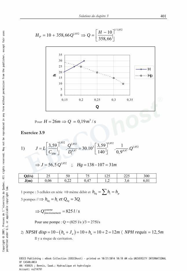
1,852 1010 358,66358,66PHH Q Q −⎡ ⎤= + ⇒ = ⎢ ⎥⎣ ⎦
Pour 326 0,19 /H m Q m s= ⇒ =
Exercice 3.9
1) 1,852 1,8521,852
3 1,8524,87 4,87
1
3,59 3,59 1. 30.10 . .140 0,9HW
QJ L QC D
⎡ ⎤ ⎡ ⎤= =⎢ ⎥ ⎢ ⎥⎣ ⎦⎣ ⎦
1,85256,5 ; 138 107 31J Q Hg m⇒ = = − =
Q(l/s) 25 50 75 125 225 300 J(m) 0,06 0,22 0,47 1,2 3,6 6,01
1 pompe : 3 cellules en série ⇒ même débit et éq i ph h h= =∑
3 pompes // ⇒ 3éq i éq ih h et Q Q= =
825 /systeme
fonctionnementQ l s⇒ = Pour une pompe : Q = (825 l/s )/3 = 275l/s 2) ( )10 10 10 2 12 12,5a a aNPSH disp h J h m NPH requis m= − + = + = + = ⟨ = Il y a risque de cavitation.
0
5
10
15
20
25
30
35
0,15 0,2 0,25 0,3 0,35
Q
h
HHp
Copyright © 2007. Presses de l''niversite du Quebec. All rights reserved. May not be reproduced in any form without permission from the publisher, except fair uses
permitted under U.S. or applicable copyright law.
EBSCO Publishing : eBook Collection (EBSCOhost) - printed on 10/27/2014 10:19 AM via UNIVERSITY INTERNATIONALOF CASABLANCAAN: 438925 ; Bennis, Saad.; Hydraulique et hydrologieAccount: ns214791

Solutions du chapitre 5 402
EXERCICES DU CHAPITRE 5 Exercice 5.1 40,013; 5 ; 1 5.10n on B m h m S −= = = = 1) Selon l’équation (5.13)
2 /3 1/ 2H
AQ R Sn
=
D’après le tableau 5.1, le rayon hydraulique est :
5 1 52 5 2 1 7
nH
n
B hRB h
⋅ ⋅= = =
+ + ⋅
( )2/3
1/ 24 35 1 5 . 5 10 6,87 /0,013 7
Q m s−⋅ ⎛ ⎞= ⋅ =⎜ ⎟⎝ ⎠
2) 2/3
1/ 22 13,74
2n n
n
B y B yQ Sn B y
⎛ ⎞⋅ ⋅= = ⋅ ⋅⎜ ⎟+⎝ ⎠
2 /3
1/ 25 513,74 0,00050,013 5 2
n n
n
y yy
⎛ ⎞= ⋅ ⋅⎜ ⎟+⎝ ⎠
2
355 7,99 05 2
nn
n
yyy
⎛ ⎞⋅ − =⎜ ⎟+⎝ ⎠
On trouve par itérations successives : 1,62ny m= Exercice 5.2 1) D’après l’équation (5.13) :
2/3 1/ 2H
AQ R Sn
=
D’après le tableau (5.1) :
( ) ( )2 2
n nn n H
n
b y yA b y y et R
b y+
= + =+
Copyright © 2007. Presses de l''niversite du Quebec. All rights reserved. May not be reproduced in any form without permission from the publisher, except fair uses
permitted under U.S. or applicable copyright law.
EBSCO Publishing : eBook Collection (EBSCOhost) - printed on 10/27/2014 10:19 AM via UNIVERSITY INTERNATIONALOF CASABLANCAAN: 438925 ; Bennis, Saad.; Hydraulique et hydrologieAccount: ns214791

Solutions du chapitre 5
403
( ) ( ) 2/3
1/ 26 610 0,001
0,022 6 2.8284n n n n
n
y y y yy
+ ⋅ + ⋅⎛ ⎞= ⋅ ⋅⎜ ⎟+⎝ ⎠
( ) ( ) 2/36
6,9570 66 2,8284
n nn n
n
y yy y
y+⎛ ⎞
= + ⋅ ⎜ ⎟+⎝ ⎠
Par essais successifs : 1,092ny m=
2) En utilisant de nouveau l’équation (5.13) avec y = 2,184m : (6 2,184) 2,184 17,8739A m= + ⋅ =
(6 2,184) 2,184 1,46786 2,8284 2,184HR m+ ⋅
= =+ ⋅
( )2/3 1/ 2 317,8739 1,4678 0,001 33,2 /0,022
Q m s= ⋅ ⋅ =
Exercice 5.3 D’après le tableau 5.1 :
(6 2 )A y y= + et ( )6 26 2 5H
y yR
y+
=+
Selon l’équation (5.12) :
2 /3 1/ 21HV R S
n= et Q = AV
On peut donc calculer V et Q pour différentes valeurs de y
y(m) A(m2) V(m/s) Q(m3/s)
0,3 1,98 0,467 0,9240,9 7,02 0,882 6,1891,5 13,5 1,164 15,712,1 21,42 1,394 29,853 36 1,687 60,744 56 1,973 110,486
Copyright © 2007. Presses de l''niversite du Quebec. All rights reserved. May not be reproduced in any form without permission from the publisher, except fair uses
permitted under U.S. or applicable copyright law.
EBSCO Publishing : eBook Collection (EBSCOhost) - printed on 10/27/2014 10:19 AM via UNIVERSITY INTERNATIONALOF CASABLANCAAN: 438925 ; Bennis, Saad.; Hydraulique et hydrologieAccount: ns214791

Solutions du chapitre 5 404
Exercice 5.4
222
n nn n n
y yA b y b y y⋅ ⋅= ⋅ + = ⋅ + d’où :
2n
n
A yby−
=
3
210 / 101 /
Q m sA mV m s
= = =
Pour yn = 1,0m 210 1 1 9
1b b m−
= = =
Exercice 5.5 Le cas de la conduite pleine permet de calculer S par l’équation (5.13) :
2
2 /3 1/ 21 ;4 4P H HD A DQ A R S avec A R
n Pπ
= = = =
( )222 2 2 2
4/3 4 /32 4/3 2 4 2 4
0,014 0,1000,0114
3,14 0,305 0,30516 4 16 4
n Q n QSA R D Dπ
⋅= = = =
⋅⎛ ⎞ ⎛ ⎞⋅ ⋅⎜ ⎟ ⎜ ⎟⎝ ⎠ ⎝ ⎠
0,0114S = Conduite 75 % pleine : 0,75 229ny D mm= ⋅ =
Vitesse -vs- profondeur
0
0,5
1
1,5
2
0 1 2 3 4
y (m)
V (m
/s)
Débit -vs- profondeur
020406080
100120
0 1 2 3 4
y (m)
Q (m
3/s)
Copyright © 2007. Presses de l''niversite du Quebec. All rights reserved. May not be reproduced in any form without permission from the publisher, except fair uses
permitted under U.S. or applicable copyright law.
EBSCO Publishing : eBook Collection (EBSCOhost) - printed on 10/27/2014 10:19 AM via UNIVERSITY INTERNATIONALOF CASABLANCAAN: 438925 ; Bennis, Saad.; Hydraulique et hydrologieAccount: ns214791

Solutions du chapitre 5
405
20,100 1,3687 /0,305
4
PP
QV m sA π
= = =⋅
Selon le tableau 5.3, 1,135P
VV
=
Donc 1,1325 1,3687 / 1,55 /V m s m s= ⋅ = 1,55 /V m s= * Conduite 30 % pleine : 0,3. 91,5ny D mm= =
0,776 0,776 1,3687 / 1,0621 /V V m s m sVp
= ⋅ = ⋅ =
1,06 /V m s= Exercice 5.6
0,75 5.3 0,91p
Qh D TableauQ
= ⇒ ⇒ = ⇒ 30,14 0,154 /0,91pQ m s= =
3 min minmin 0,03 / 0,195 5.3 0,776
p p
Q VQ m s tableauQ V
= ⇒ = ⇒ ⇒ =
ou min 0,6 / 0,77 /pV m s V m s= ⇒ =
2
20,154 0,1980,77 4
p
p
Q DA mV
π= = = = ⇒ 0,5D m=
Calcul de S en utilisant l’équation (5.12) :
2
32/3 2 /3
0,015 0,77 2,1 100,54
H
n VpSR
−
⎛ ⎞⎜ ⎟⎛ ⎞⋅ ⋅⎜ ⎟= = = ⋅⎜ ⎟ ⎜ ⎟⎛ ⎞⎝ ⎠ ⎜ ⎟⎜ ⎟⎜ ⎟⎝ ⎠⎝ ⎠
Copyright © 2007. Presses de l''niversite du Quebec. All rights reserved. May not be reproduced in any form without permission from the publisher, except fair uses
permitted under U.S. or applicable copyright law.
EBSCO Publishing : eBook Collection (EBSCOhost) - printed on 10/27/2014 10:19 AM via UNIVERSITY INTERNATIONALOF CASABLANCAAN: 438925 ; Bennis, Saad.; Hydraulique et hydrologieAccount: ns214791

Solutions du chapitre 5 406
32,1.10S −= Selon le tableau 5.3, le débit maximum à surface libre est
3maxmax1,0745 0,166 /
p
Q donc Q m sQ
= =
Exercice 5.7
Indices utilisés : c pour conduite à section circulaire et r pour conduite à section rectangulaire.
( )2/3 2/3
25.13 , :
2 .
r c
f
c rHc Hr
c r
Q Qutilisant simplifiant par S
A AR Rn n
= ⋅
× =
2 21,54 1,8627 0,385
4 4 4c
c HcD DA et Rπ π⋅ ⋅
= = = = =
1,54r r rA b y y= ⋅ = ⋅
Selon le tableau 5.1 : 1,542 1,54 2
r rHr
r r
b y yRb y y
⋅ ⋅= =
+ +
Donc 2 /3
2 /32 1,8627 1,54 1,540,3850,025 0,012 1,54 2
r r
r
y yy
⎛ ⎞⋅ ⋅ ⋅⋅ = ⋅⎜ ⎟+⎝ ⎠
Soit : 21,54 0,9634 0,7418 0
1,074r r
r
y y
y m
− − =
=
Exercice 5.8 35 / , 0,013Q m s n= = 4B m=
Copyright © 2007. Presses de l''niversite du Quebec. All rights reserved. May not be reproduced in any form without permission from the publisher, except fair uses
permitted under U.S. or applicable copyright law.
EBSCO Publishing : eBook Collection (EBSCOhost) - printed on 10/27/2014 10:19 AM via UNIVERSITY INTERNATIONALOF CASABLANCAAN: 438925 ; Bennis, Saad.; Hydraulique et hydrologieAccount: ns214791

Solutions du chapitre 5
407
a) Le débit unitaire est 3
25 / 1,25 /4
Q m sq m sb m
= = =
Selon l’équation (5.25) :1/3 1/32 21, 25 0,5421
9,81cqy mg
⎛ ⎞ ⎛ ⎞= = =⎜ ⎟ ⎜ ⎟
⎝ ⎠ ⎝ ⎠
0,54cy m= b) D’après (5.28) 2,3 /c cV g y m s= ⋅ =
2,3 /cV m s=
c) D’après (5.31)
2
23
0,0028c
c
c H
nQSA R
⎛ ⎞⎜ ⎟= =⎜ ⎟⎝ ⎠
0,0028cS = Exercice 5.9 1) En (3) : 35 10 1 50 /Q V A m s= ⋅ = ⋅ ⋅ = La charge totale en 3 :
2 2
33 3
51 2, 272 2.9,81VE y m
g= + = + =
Par la conservation d’énergie entre 2 et 3
22
322 32 2
VVy Z yg g
+ + Δ = +
L’écoulement est critique en 2 si 2 0dEdy
=
2 2
22 2 2 2 2 3
2
02
Q dE QE y etB y g dy B gy
= + = − =⋅ ⋅
2 2
332 2 2
50 1,36610 9,81c
Qy mB g
= = =⋅ ⋅
Copyright © 2007. Presses de l''niversite du Quebec. All rights reserved. May not be reproduced in any form without permission from the publisher, except fair uses
permitted under U.S. or applicable copyright law.
EBSCO Publishing : eBook Collection (EBSCOhost) - printed on 10/27/2014 10:19 AM via UNIVERSITY INTERNATIONALOF CASABLANCAAN: 438925 ; Bennis, Saad.; Hydraulique et hydrologieAccount: ns214791

Solutions du chapitre 5 408
1,366cy m=
2
3 2 2 2
502, 27 1,36610 1,366 2 9,81
E E z Z= + Δ = = + + Δ⋅ ⋅ ⋅
2, 27 2,049 0,221Z m m mΔ = − = 0, 221z mΔ = 2) Selon (5.22), le nombre de Froude en 1 est :
2 2 2
23 3 3 2 3
1 1
Q B Q B QFrgA gB y g B y
⋅= = =
⋅ ⋅ ⋅
Selon la conservation d’énergie entre 1 et 2 : 1 2 3 2, 27E E E m= = =
35,0 / 1,0 10,0 50 /Q V A m s m m m s= ⋅ = ⋅ ⋅ =
2 2
1 12 2 2 21 1
502 10 2 9,81Qy y
B g y y+ = +
⋅ ⋅ ⋅ ⋅ ⋅ ⋅
1 21
1, 274 2,27yy
+ = 1 1y m=
2
22 3
50 2,559,81 10 1,0
Fr = =⋅ ⋅
1,60 1rF = >
Régime torrentiel dans la section 1 Exercice 5.10
1) En (1) : 1 11 1 1 1
1 1
5.1:2H
B yA B y et du tableau RB y
⋅= ⋅ =
+ ⋅
D’après (5.22) : 2 2
2 13 2 3
1 1
Q B QFrg A g B y
= =⋅ ⋅ ⋅
Selon (5.13) 2 /3
2 /3 1/ 2 1/ 21 10 1 1 0
1 1
1 12 2H
B yQ AR S B y Sn B y
⎛ ⎞= = ⋅ ⋅⎜ ⎟+ ⋅⎝ ⎠
Copyright © 2007. Presses de l''niversite du Quebec. All rights reserved. May not be reproduced in any form without permission from the publisher, except fair uses
permitted under U.S. or applicable copyright law.
EBSCO Publishing : eBook Collection (EBSCOhost) - printed on 10/27/2014 10:19 AM via UNIVERSITY INTERNATIONALOF CASABLANCAAN: 438925 ; Bennis, Saad.; Hydraulique et hydrologieAccount: ns214791

Solutions du chapitre 5
409
2/3
411
1
1 1010 10 4 100,02 10 2
yyy
−⎛ ⎞= ⋅ ⋅ ⋅ ⋅⎜ ⎟+⎝ ⎠
211 1 1
1
101 10 2 10 010 2
yy soit y yy
⎛ ⎞= ⋅ − − =⎜ ⎟+⎝ ⎠
1 1,1y m=
2
21 2 3
10 0,0769,81 10 1,1
Fr = =⋅ ⋅
et 1 0, 275 11
Frécoulement fluvial en
= <
En 2, il faut que l’écoulement soit critique, donc 2 1Fr =
Comme en 1,
( )2
2 2 2 32 2 22 3
2 2
1QFr et Q g B yg B y
= = = ⋅ ⋅⋅ ⋅
Selon la conservation de l’énergie :
2 2
1 2 22 2 2 211 1 2 22 2 c
Q QE y E y Eg B y g B y
= + = = + =⋅ ⋅ ⋅ ⋅
Donc 2
2 2
101,1 1,1422 9,81 10 1,1cE m m= + =
⋅ ⋅ ⋅
Selon (5.27) : 3 2 1,142 0,762 3c c cE y donc y m⋅
= ⋅ = = 0,76cy m=
D’après (5.25) : 2 2 2 2
23 3 2 3
/c
c
q Q B Qy donc Bg g gy
= = =
2 4,82B m=
2) Pour 1 22 2, 41
2BB m= =
Selon (5.27) : 1 12
3 1,812C cE y m= =
Copyright © 2007. Presses de l''niversite du Quebec. All rights reserved. May not be reproduced in any form without permission from the publisher, except fair uses
permitted under U.S. or applicable copyright law.
EBSCO Publishing : eBook Collection (EBSCOhost) - printed on 10/27/2014 10:19 AM via UNIVERSITY INTERNATIONALOF CASABLANCAAN: 438925 ; Bennis, Saad.; Hydraulique et hydrologieAccount: ns214791
Solutions du chapitre 5 410
Il faut que
( ) ( ) ( )
2 21 1 1 11 1 12 22 1 2 1
1 1 1
10 1,812 2 9,81 10
CQE E y y m
g B y y= = + = + =
⋅ ⋅ ⋅ ⋅
( ) ( )3 21 11 11,81 0,051 0y y− ⋅ + = 1
1 1,79y m=
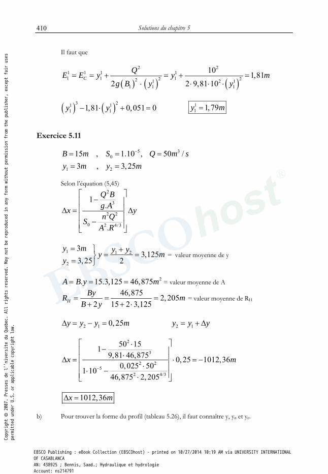
Exercice 5.11
5 3
0
1 2
15 , 1.10 , 50 /3 , 3,25
B m S Q m sy m y m
−= = == =
Selon l’équation (5,45)
2
3
2 2
0 2 4/3
1.
.
Q Bg Ax yn QS
A R
⎡ ⎤−⎢ ⎥
⎢ ⎥Δ = Δ⎢ ⎥−⎢ ⎥⎣ ⎦
1 1 2
2
33,125
3, 25 2y m y yy my
= ⎫ += =⎬= ⎭
= valeur moyenne de y
2. 15.3,125 46,875A B y m= = = = valeur moyenne de A
46,875 2,205
2 15 2 3,125HByR m
B y= = =
+ + ⋅ = valeur moyenne de RH
2 1 0, 25y y y mΔ = − = 2 1y y y= + Δ
2
3
2 25
2 4/3
50 1519,81 46,875 0, 25 1012,36
0,025 501 1046,875 2, 205
x m−
⎡ ⎤⋅−⎢ ⎥⋅⎢ ⎥Δ = ⋅ = −
⋅⎢ ⎥⋅ −⎢ ⎥⋅⎣ ⎦
1012,36x mΔ = b) Pour trouver la forme du profil (tableau 5.26), il faut connaître y, yn et yc.
Copyright © 2007. Presses de l''niversite du Quebec. All rights reserved. May not be reproduced in any form without permission from the publisher, except fair uses
permitted under U.S. or applicable copyright law.
EBSCO Publishing : eBook Collection (EBSCOhost) - printed on 10/27/2014 10:19 AM via UNIVERSITY INTERNATIONALOF CASABLANCAAN: 438925 ; Bennis, Saad.; Hydraulique et hydrologieAccount: ns214791
Solutions du chapitre 5
411
Utilisant (5.13) :
2/32/3
0,5 2n
H nn
B ynQ A R B yS B y
⎛ ⎞⋅= ⋅ = ⋅ ⋅⎜ ⎟+ ⋅⎝ ⎠
2/3
5
150,025 5015 21,0 10 15
nn
n
yyy−
⎛ ⎞⋅⋅= ⋅⎜ ⎟+ ⋅⋅ ⋅ ⎝ ⎠
10ny m=
Pour yc, Fr = 1,0 Selon (5.22) :
( )
2 22
331rc
Q B Q BFg A g B y
⋅ ⋅= = =
⋅ ⋅ ⋅
1/3 1/32 2
3 2
50 1,049,81 15c
Qy mg B
⎛ ⎞ ⎛ ⎞= = =⎜ ⎟ ⎜ ⎟⋅ ⋅⎝ ⎠ ⎝ ⎠
1,04cy m=
n cy y y> > : il s’agit du profil M2 sur le tableau 5.26
2 'y est donc vers l amont
Exercice 5.12 Géométrie du fond du canal : Z2 = 25m Zj = Z2 + S2 x L2 = 25 + 0,001 x 1500 = 26,5m Z1 = Xj + S1 x L1 = 26,5 + 0,005 x 300 = 28,0m Valeurs connues : y1 = 30,0m – 28,0m = 2,0m y2 = 27,5m – 25,0m = 2,5m L’écoulement est critique à l’entrée du canal : 1 2,0cy y m= =
Copyright © 2007. Presses de l''niversite du Quebec. All rights reserved. May not be reproduced in any form without permission from the publisher, except fair uses
permitted under U.S. or applicable copyright law.
EBSCO Publishing : eBook Collection (EBSCOhost) - printed on 10/27/2014 10:19 AM via UNIVERSITY INTERNATIONALOF CASABLANCAAN: 438925 ; Bennis, Saad.; Hydraulique et hydrologieAccount: ns214791

Solutions du chapitre 5 412
Selon (5.25) : 1/ 32
c
qy
g=
⎡ ⎤⎢ ⎥⎣ ⎦
d’où ( ) ( )1/ 2 1/ 23 39,81 2cq g y= ⋅ = ⋅
( )1/ 23 39, 0 9,81 2 79, 73 /Q B q m s= ⋅ = ⋅ ⋅ =
La figure 5.14 donne y/b en fonction de 2 / 3 8 / 3/HAR b .
De (5.13) : ( )2 / 3 1/ 2/ HA nQ R S= . Donc ( )2 / 3 8 / 3 8 / 3 1/ 2/ /HAR b nQ b S=
Dans la section 1, 8 / 3 1/ 2 8 / 3 1/ 2
1
0, 015 79, 730, 048
9,0 0, 005nQ
b S⋅
= =⋅ ⋅
De la figure 5.14, y/b = 0,17. Donc 1
1,53Ny m= Donc, l’écoulement est torrentiel dans la section 1.
Dans la section 2, 8 / 3 1/ 2 8 / 3 1/ 2
2
0, 015 79, 730,108
9, 0 0, 001nQ
b S⋅
= =⋅ ⋅
De la figure 5.14, y/b = 0,28. Donc 2
2,52Ny m= Donc l’écoulement est fluvial dans la section 2. L’allure de la surface libre est montrée schématiquement sur la figure ci-jointe.
1,5m
lac 1
lac 2torrentiel
fluvial
Section 1 Section 2
y =2mc y =2mc
y = 2,52mN2
y = 1,53mN1
Copyright © 2007. Presses de l''niversite du Quebec. All rights reserved. May not be reproduced in any form without permission from the publisher, except fair uses
permitted under U.S. or applicable copyright law.
EBSCO Publishing : eBook Collection (EBSCOhost) - printed on 10/27/2014 10:19 AM via UNIVERSITY INTERNATIONALOF CASABLANCAAN: 438925 ; Bennis, Saad.; Hydraulique et hydrologieAccount: ns214791

Solutions du chapitre 5
413
Exercice 5.13 La profondeur normale peut être calculée à partir de l’équation (5.13) en substituant
2
nn H
n
B yA B y et R
B y⋅
= ⋅ =+ ⋅
Ainsi :
2/31/ 2
2n n
fn
B y B yQ Sn B y
⎛ ⎞⋅ ⋅= ⋅ ⋅⎜ ⎟+ ⋅⎝ ⎠
(a) Supposant Sf = S0 = 0,009 et groupant les termes connus à gauche, (a) donne :
2/31015 0,025
10 210 0,0090,39528
nn
n
yyy
⎛ ⎞⋅⋅= ⋅⎜ ⎟+ ⋅⋅ ⎝ ⎠
=
(b) On résout (b) par essais successifs et on obtient 0,60ny m= Selon l’équation (5.25), la profondeur critique est:
( )
1/31/3 22 15 /100,612
9,81cqy mg
⎛ ⎞⎛ ⎞= = =⎜ ⎟⎜ ⎟ ⎜ ⎟⎝ ⎠ ⎝ ⎠
Selon les données, yref = y0 = yn + 4,0m = 4,60m (voir paragraphe 5.7.3.3). Donc yn = yc : pente critique; yref > yc : courbe de remous de type C1 (figure 5.27) Suivant la procédure pour yref connu à l’aval (au contact avec le lac), avec 0,50y mΔ =
1- y1 = yref = 4,60m, pour x = 0 2- y2 = y1 – 0,50m = 4,10m 3- ym = (y1 + y2)/2 = 4,35m 4- Am = Bym = 10m· 4,35m = 43,50m2 5- RHm = Am/B+2ym = 2,326m 6- On calcule Δx par (5.45) :
2
3
1 2 2
2 4/3
15 101
9,81 43,50,5 55, 4010, 025 15
0, 00943,5 2,326
x m
⋅−
⋅Δ = ⋅ =⋅
−⋅
⎡ ⎤⎢ ⎥⎢ ⎥⎢ ⎥⎢ ⎥⎣ ⎦
7- x = x + Δx = 0 + 55,401m = 55,401m 8- y2 = y1 = 4,10m 9- on recommence à l’étape 2 jusqu’à de qu’on atteigne y = yn
Copyright © 2007. Presses de l''niversite du Quebec. All rights reserved. May not be reproduced in any form without permission from the publisher, except fair uses
permitted under U.S. or applicable copyright law.
EBSCO Publishing : eBook Collection (EBSCOhost) - printed on 10/27/2014 10:19 AM via UNIVERSITY INTERNATIONALOF CASABLANCAAN: 438925 ; Bennis, Saad.; Hydraulique et hydrologieAccount: ns214791

Solutions du chapitre 5 414
Le tableau suivant montre les étapes de calcul :
y1 y2 ym Am RHm Δx x 4,6 4,1 4,35 43,5 18,7 55,401 55,401 4,1 3,6 3,85 38,5 17,7 55,332 110,733 3,6 3,1 3,35 33,5 16,7 55,217 165,950 3,1 2,6 2,85 28,5 15,7 55,005 220,955 2,6 2,1 2,35 23,5 14,7 54,574 275,529 2,1 1,6 1,85 18,5 13,7 53,543 329,072 1,6 1,1 1,35 13,5 12,7 50,377 379,449 1,1 0,6 0,85 8,5 11,7 34,808 414,258
La figure suivante montre la courbe de remous (Note : les valeurs des x ont été ajustées de manière à représenter le lac à droite)
Courbe de remous
0
1
2
3
4
5
6
-200 0 200 400 600
X (m)
Y (m
)
fondsurf.Yolac
Copyright © 2007. Presses de l''niversite du Quebec. All rights reserved. May not be reproduced in any form without permission from the publisher, except fair uses
permitted under U.S. or applicable copyright law.
EBSCO Publishing : eBook Collection (EBSCOhost) - printed on 10/27/2014 10:19 AM via UNIVERSITY INTERNATIONALOF CASABLANCAAN: 438925 ; Bennis, Saad.; Hydraulique et hydrologieAccount: ns214791
Solutions du chapitre 5
415
Exercice 5.14
Conduite 4-3 Débit pour conduite pleine, selon l’équation (5.17) :
8/3 1/ 2 30,3117 2,44 0,0025 12,94 /0,013pQ m s= ⋅ ⋅ =
15,0 1,16
12,94p
= = , donc il y a mise en charge
Selon l’équation (5.15b) :
2 2
8/3 8/3
0,013 15 0,0033610,3117 0,3116 2, 44f
n QSD
⋅ ⋅⎛ ⎞ ⎛ ⎞= = =⎜ ⎟ ⎜ ⎟⋅ ⋅⎝ ⎠ ⎝ ⎠
500,0 0,003361 1,68fH L S m mΔ = ⋅ = ⋅ = Niveau d’eau en 3 : 27,0m + 1,68m = 28,68m (pas d’inondation en 3).
Conduite 3-1
8/3 1/ 2 30,3117 1,37 0,0015 2,15 /0,013pQ m s= ⋅ ⋅ =
6,0 2,82,15p
= = , donc il y a mise en charge
2
8/3
0,013 6,0 0,01680,3117 1,37fS ⋅⎛ ⎞
= =⎜ ⎟⋅⎝ ⎠
100,0 0,0168 1,68H m mΔ = ⋅ = Niveau de l’eau en 1 : 18,68m + 1,68m = 30,36m (pas d’inondation en 1)
Copyright © 2007. Presses de l''niversite du Quebec. All rights reserved. May not be reproduced in any form without permission from the publisher, except fair uses
permitted under U.S. or applicable copyright law.
EBSCO Publishing : eBook Collection (EBSCOhost) - printed on 10/27/2014 10:19 AM via UNIVERSITY INTERNATIONALOF CASABLANCAAN: 438925 ; Bennis, Saad.; Hydraulique et hydrologieAccount: ns214791

Solutions du chapitre 5 416
Conduite 3-2
8/3 1/ 2 30,3117 0,915 0,004 1,197 /0,013pQ m s= ⋅ ⋅ =
4 3,35
1,197p
= = , donc il y a mise en charge
2
8/3
0,013 4,0 0,04470,3117 0,915fS ⋅⎛ ⎞
= =⎜ ⎟⋅⎝ ⎠
100,0 0,0447 4,47H m mΔ = ⋅ = Niveau de l’eau en 2 : 26,68m + 4,47m = 31,15m Le niveau du sol en 2 étant 30,5m, il y a une inondation de 0,65m. Les profils piézométriques sont montrés sur la figure ci-jointe :
Copyright © 2007. Presses de l''niversite du Quebec. All rights reserved. May not be reproduced in any form without permission from the publisher, except fair uses
permitted under U.S. or applicable copyright law.
EBSCO Publishing : eBook Collection (EBSCOhost) - printed on 10/27/2014 10:19 AM via UNIVERSITY INTERNATIONALOF CASABLANCAAN: 438925 ; Bennis, Saad.; Hydraulique et hydrologieAccount: ns214791

Solutions du chapitre 5
417
Échelle horizontale = 100 fois échelle verticale
2425
262728
2930
313233
344 13
Cours d’eau
Lignepiézométrique
Élév
atio
n (m
)
500 mètres100m
2425
262728
2930
313233
344 23
Cours d’eau
Élév
atio
n (m
)
500 mètres 100m
Copyright © 2007. Presses de l''niversite du Quebec. All rights reserved. May not be reproduced in any form without permission from the publisher, except fair uses
permitted under U.S. or applicable copyright law.
EBSCO Publishing : eBook Collection (EBSCOhost) - printed on 10/27/2014 10:19 AM via UNIVERSITY INTERNATIONALOF CASABLANCAAN: 438925 ; Bennis, Saad.; Hydraulique et hydrologieAccount: ns214791

Solutions du chapitre 5 418
Choix des diamètres pour éliminer les mises en charge et l’inondation. On suppose Sf = S0.
Conduite 4-3 Pour une conduite pleine, on a de l’équation (5.17) :
3/8
1/ 20,3117p
pf
n QD
S
⎛ ⎞⋅= ⎜ ⎟⎜ ⎟⋅⎝ ⎠
(c)
3/8
1/ 2
15,0 0,013 2,580,3117 0,0025pD m⋅⎛ ⎞
= =⎜ ⎟⋅⎝ ⎠
Le diamètre disponible est D = 2,745m pour lequel Qp est :
8/3 1/ 2 30,3117 2,745 0,0025 17,71 /0,013pQ m s= ⋅ ⋅ =
15,0 0,8517,71p
= =
À l’aide du tableau 5.3, on obtient y/D = 0,707 et donc y = 0,707· 2,745 = 1,94m
La profondeur de l’eau au point 3 dans la nouvelle conduite de diamètre 2,745m est donc de 1,94m. L’écoulement est donc à surface libre au point 3 et il n’y a plus de mise en charge. La conduite sera pleine à partir d’un point entre 3 et 4.
Conduite 3-1 Procédant comme précédemment, Dp = 2,013m. Diamètre disponible = 2,135m. Pour ce diamètre Qp = 7,018m3/s ; Q/Qp = 0,855; y/D = 0,71 Profondeur de l’eau en 1 : y = 1,52m. L’écoulement est à surface libre et il n’y a plus de mise en charge.
Conduite 3-2 Comme plus haut, Dp = 1,439m Diamètre disponible = 1,525m. Pour ce diamètre Qp = 4,672m3/s ; Q/Qp = 0,86; y/D = 0,72 Profondeur de l’eau en 1 : y = 1,1m. L’écoulement est à surface libre et il n’y a plus de mise en charge.
Copyright © 2007. Presses de l''niversite du Quebec. All rights reserved. May not be reproduced in any form without permission from the publisher, except fair uses
permitted under U.S. or applicable copyright law.
EBSCO Publishing : eBook Collection (EBSCOhost) - printed on 10/27/2014 10:19 AM via UNIVERSITY INTERNATIONALOF CASABLANCAAN: 438925 ; Bennis, Saad.; Hydraulique et hydrologieAccount: ns214791

Solutions du chapitre 5
419
Exercice 5.15 L’équation de Bernoulli s’écrit entre les points 0 et 1, en négligeant les pertes de charge :
( )2 2
0 10 1 1 14 0 4; 2 4
2 2V V
H y donc V g yg g
+ = + = + = = − (1)
1 1 1 1
1 1
11
10 101
Q V A V ByV y
Vy
= == ×
=
(2)
En substituant (2) dans (1) on obtient :
3 21 1
3 21 1
2 8 1 0
19.62 78.48 1 0
g y g y
y y
− + =
− + =
Dont la solution est 1 0,115y m=
On trouve y2 en utilisant (5.51) :
2
22
0,115 10,115 0,10194
2 9,81y
y+
⋅ = =⎛ ⎞⎜ ⎟⎝ ⎠
soit : 2
2 20,115 1,773 0y y+ − = La racine positive de cette équation donne y2 = 1,275m
H =4,0mO
V /2yO2
V /2y12
(0) (1)
Copyright © 2007. Presses de l''niversite du Quebec. All rights reserved. May not be reproduced in any form without permission from the publisher, except fair uses
permitted under U.S. or applicable copyright law.
EBSCO Publishing : eBook Collection (EBSCOhost) - printed on 10/27/2014 10:19 AM via UNIVERSITY INTERNATIONALOF CASABLANCAAN: 438925 ; Bennis, Saad.; Hydraulique et hydrologieAccount: ns214791

Solutions du chapitre 6 420
EXERCICES DU CHAPITRE 6 Exercice 6.1 Selon la formule de Francis (6.16)
3/ 20, 415 25HQ g L H⎛ ⎞= ⋅ ⋅ ⋅ − ⋅⎜ ⎟
⎝ ⎠
3/ 2 30,300,415 2 9,81 5 0,30 1,492 /5
Q m s⎛ ⎞= ⋅ ⋅ ⋅ − ⋅ =⎜ ⎟⎝ ⎠
Selon la formule de Hégley On calcule μ par (6.17) :
( )
20,0027 5 3 5 0,30
0, 405 0, 03 1 0,55 0, 4480,30 5 3 0,30 1, 0
μ− ⋅
= + − ⋅ ⋅ + ⋅ =⋅ +
⎡ ⎤⎛ ⎞⎡ ⎤ ⎢ ⎥⎜ ⎟⎢ ⎥⎣ ⎦ ⎢ ⎥⎝ ⎠⎣ ⎦
Selon l’équation (6.15) :
3/ 2 30, 448 5,0 2 9,81 0,30 1,630 /Q m s= ⋅ ⋅ ⋅ ⋅ = Exercice 6.2 Selon la formule de Thomson (6.24) :
5/ 21, 42Q H= ⋅ donc : 2/5
1, 42QH ⎛ ⎞
= ⎜ ⎟⎝ ⎠
2/5
0,060 0, 2821, 42
H m⎛ ⎞= =⎜ ⎟
⎝ ⎠
Exercice 6.3
Formule de Francis : 3
20.415 2Q L g H=
Quand Q = 0,15m³/s H= 0,3 m
Comme 3
0.415 22
Q HL g
Q HΔ Δ
= ×
Copyright © 2007. Presses de l''niversite du Quebec. All rights reserved. May not be reproduced in any form without permission from the publisher, except fair uses
permitted under U.S. or applicable copyright law.
EBSCO Publishing : eBook Collection (EBSCOhost) - printed on 10/27/2014 10:19 AM via UNIVERSITY INTERNATIONALOF CASABLANCAAN: 438925 ; Bennis, Saad.; Hydraulique et hydrologieAccount: ns214791
Solutions du chapitre 6
421
Donc 30.415 2
2H
Q L g QH
ΔΔ = × ×⎛ ⎞
⎜ ⎟⎝ ⎠
23 10
0.415 0.5 2 9.81 0.152 0.30
−
= × × × × × ×
30.0068 sQ mΔ =
Soit 4.54%QQ
Δ=
Exercice 6.4 On calcule Cq selon (6.29) :
0,65 0,65 0,4331,01 12,0
qC Hz
= = =+ +
Δ
Le débit est obtenu de (6.28) : 3/ 2 3/ 2 31,7 1,7 0, 433 5,0 1 2,17 /qQ C L H m s= ⋅ ⋅ ⋅ = ⋅ ⋅ ⋅ =
Copyright © 2007. Presses de l''niversite du Quebec. All rights reserved. May not be reproduced in any form without permission from the publisher, except fair uses
permitted under U.S. or applicable copyright law.
EBSCO Publishing : eBook Collection (EBSCOhost) - printed on 10/27/2014 10:19 AM via UNIVERSITY INTERNATIONALOF CASABLANCAAN: 438925 ; Bennis, Saad.; Hydraulique et hydrologieAccount: ns214791

Solutions du chapitre 7 422
EXERCICES DU CHAPITRE 7
Exercice 7.1
Méthode de Thiessen, formule (7.4) :
i iS PP
A= ∑
A = 2 · 2 = 4
50 3/ 2 10 3/ 2 20 1 27,5
4mm mm mmP mm⋅ + ⋅ + ⋅
= =
Méthode arithmétique, formule (7.2) :
( )1 1 50 20 10 26,73iP P mm
n= Σ = + + =
Exercice 7.2
Selon (7.3) : i iA PP
A= ∑
Intervalle (mm) Moyenne (mm) Superficie (km2)
40 à 60 50 600 20 à 40 30 300 0 à 20 10 200
50 600 30 300 10 200 37,31100
P mm⋅ + ⋅ + ⋅= =
Copyright © 2007. Presses de l''niversite du Quebec. All rights reserved. May not be reproduced in any form without permission from the publisher, except fair uses
permitted under U.S. or applicable copyright law.
EBSCO Publishing : eBook Collection (EBSCOhost) - printed on 10/27/2014 10:19 AM via UNIVERSITY INTERNATIONALOF CASABLANCAAN: 438925 ; Bennis, Saad.; Hydraulique et hydrologieAccount: ns214791

Solutions du chapitre 7
423
Exercice 7.3
Infiltration selon Horton (7.7) :
( ) ( ) ( )0
40 2 80
1 kt
P mm mmf f
F t f t ek
∞ −∞
= × =
−= + −
( ) ( ) ( )3 240 252 25 1 54,8 ; 55
3F t e mm soit mm− ⋅−
= ⋅ + − =
Précipitations nettes = 80 55 25P F mm− = − =
Exercice 7.4
Utilisant (7.5) et supposant que φ < 20 mm/h
( ) ( ) ( ) ( ) 120 25 2 50 75 302h mmφ φ φ φ− + − + ⋅ − + − ⋅ =⎡ ⎤⎣ ⎦
Donc φ = 32mm/h , en contradiction avec l’hypothèse φ < 20 mm/h Supposant 20 ≤ φ ≤ 25
( ) ( ) ( )25 2 50 7530
2φ φ φ− + − + −
=
Donc φ = 35mm/h Ce résultat est en contradiction avec l’hypothèse de départ Supposant 25 ≤ φ ≤ 50
( ) ( )2 50 7530
2φ φ− + −
=
Donc φ = 38,33 mm/h Ce résultat est en accord avec l’hypothèse de départ
Copyright © 2007. Presses de l''niversite du Quebec. All rights reserved. May not be reproduced in any form without permission from the publisher, except fair uses
permitted under U.S. or applicable copyright law.
EBSCO Publishing : eBook Collection (EBSCOhost) - printed on 10/27/2014 10:19 AM via UNIVERSITY INTERNATIONALOF CASABLANCAAN: 438925 ; Bennis, Saad.; Hydraulique et hydrologieAccount: ns214791

Solutions du chapitre 7 424
Exercice 7.5
Pressions de vapeur (tableau 7.2) : ew1 (t = 20°c) = 2,339 kPa (à la surface de l’eau) ew2 (t = 30°c) = 4,244 kPa (à la saturation dans l’air)
Humidité relative = 2
0.34.244
a a
w
e ee
= =
Donc ea = 1,2732 kPa Évaporation journalière : Avec effet du vent (7.14) E = 3,66 (2,339 - 1,2732) · (1 + 0,062 × 30) = 11,15mm
Copyright © 2007. Presses de l''niversite du Quebec. All rights reserved. May not be reproduced in any form without permission from the publisher, except fair uses
permitted under U.S. or applicable copyright law.
EBSCO Publishing : eBook Collection (EBSCOhost) - printed on 10/27/2014 10:19 AM via UNIVERSITY INTERNATIONALOF CASABLANCAAN: 438925 ; Bennis, Saad.; Hydraulique et hydrologieAccount: ns214791

Solutions du chapitre 8
425
EXERCICES DU CHAPITRE 8
Exercice 8.1
Les données sont présentées graphiquement sur la figure suivante :
Les deux méthodes utilisées font référence à la figure 8.3.
La « méthode AB » considère comme ruissellement la partie de l’hydrogramme au-dessus de l’horizontale passant par le second point B, à partir de ce point. Selon la « méthode ACD», le ruissellement est la partie de l’hydrogramme au-dessus de la ligne ACD. Le point C est défini par l’intersection de la verticale PC passant par le débit de pointe, avec le prolongement de AB. Le point D est indiqué par une soudaine variation dans la représentation logarithmique des débits dans la partie descendante de l’hydrogramme (voir tableau 2) : il s’agit des valeurs du jour 9. En calculant les pentes des lignes AC et CD, on peut obtenir les limites inférieures de la portion de ruissellement pour la méthode ACD.
Hydrogramme, exercice 8.1(réf. Fig.8.3)
0
50
100
150
200
250
300
0 2 4 6 8 10 12 14 16
temps (jours)
débi
t Q (m
3/s)
hydrogrammePCABCBCD
P
A C
DB
Copyright © 2007. Presses de l''niversite du Quebec. All rights reserved. May not be reproduced in any form without permission from the publisher, except fair uses
permitted under U.S. or applicable copyright law.
EBSCO Publishing : eBook Collection (EBSCOhost) - printed on 10/27/2014 10:19 AM via UNIVERSITY INTERNATIONALOF CASABLANCAAN: 438925 ; Bennis, Saad.; Hydraulique et hydrologieAccount: ns214791

Solutions du chapitre 8 426
Pente de AC = (31,4 – 35)/1 = -3,6 (pente descendante) Équation de la ligne AC : Q = 35 – 3,6 · J Point C : temps = jour 3 , Q = 35 – 3,6 · 3 = 24,2 Pente de CD = (36,9 – 24,2)/(9 – 3) = 2,1167 Équation de la ligne CD : Q = 24,2 + 2,1167 · (J – 3)
Jour
J Q(m3/s méthode AB
Ruissellement (m3/s)méthode AB
méthodeACD
Ruissellement (m3/s) méthode ACD
0 35 35 0 35 01 31,4 31,4 0 31,4 02 34,3 31,4 2,9 27,8 6,53 250 31,4 218,6 24,2 225,8 4 140 31,4 108,6 26,32 113,68 5 89,6 31,4 58,2 28,43 61,17 6 57,4 31,4 26 30,55 26,85 7 43 31,4 11,6 32,67 10,33 8 37,3 31,4 5,9 34,78 2,52 9 36,9 31,4 5,5 36,9 010 35,7 31,4 4,3 35,7 011 35,1 31,4 3,7 35,1 012 34,9 31,4 3,5 34,9 013 34,8 31,4 3,4 34,8 014 34,7 31,4 3,3 34,7 015 34,6 31,4 3,2 34,6 0
Tableau 1
Jour Débit (m3/s) Logarithme Taux de variation3 250 5,524 140 4,94 0,585 89,6 4,49 0,456 57,4 4,05 0,447 43 3,76 0,298 37,3 3,61 0,159 36,9 3,608 0,00210 35,7 3,575 0,03311 35,1 3,558 0,01712 34,9 3,552 0,00613 34,8 3,549 0,00214 34,7 3,546 0,002
Tableau 2
Copyright © 2007. Presses de l''niversite du Quebec. All rights reserved. May not be reproduced in any form without permission from the publisher, except fair uses
permitted under U.S. or applicable copyright law.
EBSCO Publishing : eBook Collection (EBSCOhost) - printed on 10/27/2014 10:19 AM via UNIVERSITY INTERNATIONALOF CASABLANCAAN: 438925 ; Bennis, Saad.; Hydraulique et hydrologieAccount: ns214791

Solutions du chapitre 8
427
Exercice 8.2
Selon la méthode rationnelle (8.5), Q K C i A= ⋅ ⋅ ⋅ Scénario 1 : Tr = 15 min Qp = 60 · (15/20)· K· C· A = 45· K· C· A V = (45· K· C· A) · 20 = 900 KCA Scénario 2 : Tr = tc = 20min Qp = 50 KCA V = 50 KCA · 20 = 1000 KCA Scénario 3 : Tr = 25 min > tc Qp = 40 KCA V = 40 KCA· (20 + 5) = 1000 KCA 1º Scénario 2 a le débit de pointe le plus élevé. 2º Scénario 2 et 3 ont le volume de ruissellement le plus élevé. Exercice 8.3
L’écoulement de base est QB = 100pi3/s a) Ruissellement de surface débute entre 9 h et 10h et finit entre 17h et 18h. b) Selon la formule (7.5) : ruissellement direct (de surface) = (i – φ)· Δt ( )5 2,75 / 2po po h hφ= − ⋅ Donc, φ = 0,25po/h
Hydrogramme de crue
0
100
200
300
400
500
600
700
800
900
5 10 15 20
temps (heures)
Q (p
i.cu.
/s)
Hydrogr.
Écoul./base
Copyright © 2007. Presses de l''niversite du Quebec. All rights reserved. May not be reproduced in any form without permission from the publisher, except fair uses
permitted under U.S. or applicable copyright law.
EBSCO Publishing : eBook Collection (EBSCOhost) - printed on 10/27/2014 10:19 AM via UNIVERSITY INTERNATIONALOF CASABLANCAAN: 438925 ; Bennis, Saad.; Hydraulique et hydrologieAccount: ns214791

Solutions du chapitre 8 428
c) Débit de ruissellement = Q – QBase Lame de ruissellement en 2 heures = 5po. Pour l’hydrogramme unitaire de l’averse de 2 heures : HU2 = (Q – QBase)/5
heures Q(pi.cu./s) Ruiss. HU(2h)8 100 0 09 100 0 010 300 200 4011 500 400 8012 700 600 12013 800 700 14014 600 500 10015 400 300 6016 300 200 4017 200 100 2018 100 0 0
d) Temps de base : TB = 9h = Δt + tc
Où Δt est la durée de la pluie et tc est le temps de concentration. Donc tc = TB – Δt = 9h – 2h = 7h.
e) Pour une pluie de Δt = 8h, TB = Δt + tc = 8h + 7h = 15h Donc le ruissellement cesserait à 9h + 15h = 24h. f) En calculant l’hydrogramme unitaire de 8 heures, on constate que le débit de pointe se
produit à 16h et a la valeur unitaire de 75pi3/s. Le débit de pointe réel est donc 75pi3/s · 2,5 · 8 + QBase = 1600pi3/s.
Copyright © 2007. Presses de l''niversite du Quebec. All rights reserved. May not be reproduced in any form without permission from the publisher, except fair uses
permitted under U.S. or applicable copyright law.
EBSCO Publishing : eBook Collection (EBSCOhost) - printed on 10/27/2014 10:19 AM via UNIVERSITY INTERNATIONALOF CASABLANCAAN: 438925 ; Bennis, Saad.; Hydraulique et hydrologieAccount: ns214791
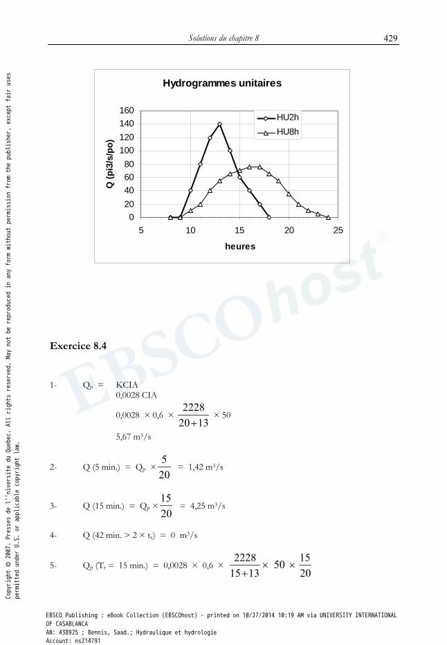
Solutions du chapitre 8
429
Exercice 8.4
1- Qp = KCIA 0,0028 CIA
0,0028 × 0,6 × 2228
20 13+ × 50
5,67 m3/s
2- Q (5 min.) = Qp ×520
= 1,42 m3/s
3- Q (15 min.) = Qp ×1520
= 4,25 m3/s
4- Q (42 min. > 2 × tc) = 0 m3/s
5- Qp (Tr = 15 min.) = 0,0028 × 0,6 × 2228 1550
15 13 20× ×
+
Hydrogrammes unitaires
020406080
100120140160
5 10 15 20 25
heures
Q (p
i3/s
/po)
HU2hHU8h
Copyright © 2007. Presses de l''niversite du Quebec. All rights reserved. May not be reproduced in any form without permission from the publisher, except fair uses
permitted under U.S. or applicable copyright law.
EBSCO Publishing : eBook Collection (EBSCOhost) - printed on 10/27/2014 10:19 AM via UNIVERSITY INTERNATIONALOF CASABLANCAAN: 438925 ; Bennis, Saad.; Hydraulique et hydrologieAccount: ns214791

Solutions du chapitre 8 430
Qp = 5,01 m3/s
6- Q (5 min) = Qp × 5
15 = 1,67 m3/s
7- Q (25 min) = 1015
Qp = 3,34 m3/s
8- Q (40 min) = 0
9- Qp (Tr = 25 min.) = 0,0028 × 0,6 × 50 × 2228
25 13+= 4,92 m3/s
10- Q (20 min.) = 4,92m3/s 11- Q (25 min.) = 4,92 m3/s 12- Q (45 min.) = 0 m3/s
Exercice 8.5 Avant :
D’après (8.11)
( ) ( )0,333 0,333
32503, 26 1,1 3, 26 1,1 0,3 109,58 min
2,5c
Lt C
S= ⋅ − ⋅ = ⋅ − ⋅ =
A = 5km2 = 500ha Selon (8.5), 30, 0028 0, 0028 0,3 500 22,19 9,32 /Q C A i m s= ⋅ ⋅ ⋅ = ⋅ ⋅ ⋅ = Utilisant la formule (5.14) :
3/8 3/8
1/ 2 1/ 2
0,014 9,32 1,710.3117 0,3117 0,01
n QD mS
⎛ ⎞⋅ ⋅⎛ ⎞= = =⎜ ⎟ ⎜ ⎟⋅ ⋅⎝ ⎠⎝ ⎠
Après :
0,3 0,5 0,5 0,9 0,6C = × + × =
Copyright © 2007. Presses de l''niversite du Quebec. All rights reserved. May not be reproduced in any form without permission from the publisher, except fair uses
permitted under U.S. or applicable copyright law.
EBSCO Publishing : eBook Collection (EBSCOhost) - printed on 10/27/2014 10:19 AM via UNIVERSITY INTERNATIONALOF CASABLANCAAN: 438925 ; Bennis, Saad.; Hydraulique et hydrologieAccount: ns214791