1

Answers to Parts B and C of the Mock Exam

Part B

Question 1

In this question we study the modelling of rational choice. At the centre of our story stand Mr

Oily who works for the energy sector (x). His income is comprised of a wage plus a bonus

which represents the company’s commitment to share the profits with its workers. The bonus is

such that it is calculated on the basis of energy prices ( xp ) and it is a fixed multiple, δ, of them

(i.e., the bonus is always Bpx ).

(a) The initial set-up is the standard case of individual choice with the exception that

income is now: BpwI x

0

00 :

(b) There is now an increase in energy prices which means that for Mr Oily the cost of

living has gone up but so has income. Will he become better or worse off?

2

It is clear enough to see that the intercept of the new budget line with the x-axis would be at a

lower level of x (i.e., his real income in terms of x fell. At the same time, his real income in

terms of y has risen. The easiest way to find out whether Mr Oily has become better or worse off

is to examine whether with the new budget line, he can carry on consuming the initial bundle A.

For A to be on both budget lines, the following must hold true:

Bpwypxp

Bpwypxp

xyx

xyx

1

00

0

0

1

0

00

0

0

0

But this means that the following must also be true:

00

0

0

1

00

0

0

0

)(

)(

wypBxp

wypBxp

yx

yx

And this will happen only when Bx 0 , which means that the factor by which the price is

multiplied to generate the profit share is the same as the quantity of energy consumed by Mr

Oily. While this is not impossible, there is something insufficiently general about it. We could

say that for sufficiently low level of consumption, the factor which multiplies the price may be

greater than the measure of energy consumed. In such a case, of course, the heavy line may

indeed go through A or even move beyond it (the diagram below). We may use this criterion to

distinguish between people who receive a small share of the profit and those who receive a

higher share. Clearly, those who receive a low share will fall into the category where A is no

longer feasible (as is in the above diagram) but someone whose share in profits is an enormous

multiplier of the price would clearly face a different situation. In other words, the larger are the

individual’s share in the profits, the more likely it is for him, or her, the benefit from the increase

in the price of energy.

3

(c) Would the family consume more or less energy products than before?

For someone whose share in the profit is sufficiently low, it is easy to see that they will consume

less. As A itself is no longer feasible, the person would have to buy less of it whether energy is

normal or inferior. In terms of the standard analysis it can clearly be seen that if energy products

are normal goods, Mr Oily will consume less of them as a result of an increase in price. The

move from A to C depicts the pure substitution effect which dictates to buy less energy products

and more of the other goods. However, as real income fell, the only way to treat energy as

normal goods would be by reducing their consumption further to the left to a point like, say, B.

The story is somewhat more complex if the multiplier factor is greater than the

consumption level:

4

Naturally, if the multiplier is sufficiently large to push the new budget well beyond A the agent

would definitely buy more energy. The more intriguing case is the one depicted above where the

multiplier factor is equal to the level of energy consumption. We can see here that as before the

substitution effect would take us from A to C. However, as real income increased, the normality

of x would mean the wish to buy more of it. This may lead us to a point like B where the final

consumption of energy would fall. It is important to note that in such a case it would necessarily

fall as a move beyond A on the heavy line is irrational.

(d) Would there be a difference in the analysis had the company simply paid the workers

a higher wages?

To make a sensibly analysis we must begin with an assumption that the income earned

by Mr Oily before and after the change is the same under the two regimes. Namely:

1

1

01

0

0

00

x

x

pwI

pwI

Evidently, in such a case there will be no difference in the position of the new budget lines nor

would there be any other difference in our analysis. Clearly, the question whether the new

budget line is to the left or the right of A depends on the relationship between the quantity of

energy consumed and the multiplier factor. But as we keep the level of income and change the

same, it will make no difference whether the agent gets his income as a bonus or as wages.

Question 2

This is a simple and straightforward question. There are no prizes for guessing that the question

is dealing with the competitive model. The specific application, which is required by this

question, is the recognition that the demand for Kiwi is comprised of two distinct groups who, as

we shall soon see, respond differently to change in the price of another good. Hence, the demand

for Kiwi is comprised of the Smoothie drinkers who treat Kiwi and Mango as complements and

the Five-a-day drinkers who treat them as gross substitute. We also have some information

5

about the price elasticity of their respective demand schedules.

(a) The initial equilibrium is therefore:

(b) We now experience an increase in the price of Mango. As the Smoothie drinkers treat the

two as complements, the increase in the price of Mango would decrease demand for Kiwi.

The Five-A-Day drinkers, on the other hand, treat the two as gross substitute and there

demand for Kiwi will therefore increase.

As we assumed that the Smoothie drinkers constitute a larger share of consumer, the overall

demand would fall. At A, there will now be excess supply of Kiwi; this will lead to a fall in price

(the move to B) and a fall in equilibrium output. Each firm will adjust its production to the new

profit maximising level (i

x1 ) where the average costs are higher than the marginal costs and

consequently, firms will be making losses. The Five-A-Day group of consumers would buy

more of the good and we cannot be sure what will happen to their overall spending. The

Smoothie groups would buy less and spend less.

(a) In the Long run, the following will occur:

D

Fx0

Sx0 0x

0

ix

P P P

Initial Set up

A AA A

S

SD

FD

iAC

iMC

0p

D

Sx0 0xF

x0

P P P

The short run effects of an increase in the price of Mango.

A AA

A

S

SD

FD

iAC

iMC

0p

'FD

'SD D’

1xSx1

Fx1

BB

B

1

ix

B

0

ix

1p

6

The loss, which firms make in the short run, will affect some by driving them out of the market.

These firms would not have sufficient assets to sustain their losses for a long period and they

will leave. As they do, supply will fall and the equilibrium price in the market will rise again.

Assuming the industry to be sufficiently small not to affect factor prices, the process will carry

on until we reach equilibrium at point C. As the price returns to its original level, each remaining

firm will produce as before (i

x0 ), where profits are at their normal rates. Altogether there are

fewer firms which explains the lower equilibrium level of output.

As price elasticity of the Smoothie drinkers is greater than unity, their spending will fall

further (relative to point B). They will also buy much less Kiwi. The Five-A-Day drinkers would

reduce their consumption relative to point B but their spending on Kiwi will increase (relative to

point B).

Question 4

This is a question about a monopolist who is facing a demand from two distinct groups of

consumers: the young who are obsessed with this fashion house because the lead singer of

Kullers wore them in concert and the older who only dress like this when no one sees them.

Clearly, the young are willing to pay higher prices for the clothes and their price elasticity would

be lower than that of the older people. The older people, on the other hand, would not be willing

to pay above a certain price, say p , and the price elasticity of their demand is likely to be much

greater than that of the young.

The first thing to establish is the shape of the demand facing the monopolist. It is clear

from the above description in the question that above p , the monopolists faces the demand

generated only by the young who have a low (though greater than unity) price elasticity. Below

that price, the combined demand generated by the two groups would yield higher price

elasticity:

D

Sx0 0xF

x0

P P P

The Long run effects of an increase in the price of Mango.

A AA

A

S

SD

FD

iAC

iMC

0p

'FD

'SD D’

1xSx1

Fx1

BB

B

1

ix

B

0

ix

1p

S’

2x

CC

Fx2

Sx2

C=C

7

Before we carry on we must ensure that it is indeed the case that the MR of the less elastic

demand would lie below the MR of the more elastic demand which is what we see above at the

point where the price equals p .

LH

LH

LH

H

H

L

L

H

H

L

L

MRMR

thenas

MRMRp

pMRpMR

11

11

11

1

11

1

]1

1[]1

1[

Which is what we have drawn in the diagram.

(a) Under which conditions would the monopolist, who cannot discriminate, sell to both

groups:

Overall demand

D

x

px

p

MR

8

Assuming, for simplicity sake that the marginal cost is constant:

We start from A which is the equilibrium when the monopolist is only selling to the first group.

To sell a unit beyond means that his marginal revenue will be below the marginal cost which

means that every additional unit reduces profit. This is true to the move between a and b. From c

to e, however, every additional unit adds to profits. Hence, whether or not the monopolist will

sell at A or B depends on whether the triangle abc is greater or smaller than the triangle cde.

(b) A new group (Onesis) becomes fashinable, comes into the market and is liked only

by young. This means that their price elasticity for the demand for Flamboyance would increase

(as there is a near substitute). We may thus face the following situation if the increase in the

young’s price elasticity was so great as to exceed those of the older people:

(c) Will he sell to the two groups?

D

x

px

p

MR

MCa

b

c

de

A

B

Overall demand

D

x

px

p

MR

9

Only if the marginal costs intersected with the MR of the two groups (depicted above).

Otherwise, he would only sell to the young.

Part C

Question 1

The government wishes to increase domestic investment and it proposes to achieve this by

offering tax incentives. People who save up to S would be exempt from tax on this amount. We

assume that the public makes full use of the offer and we are expected to explore the effects that

this would have on domestic income.

(a) The effect on the multiplier:

To see whether or not this change would affect the multiplier we must set up the model.

Although the question in not confined to a closed or open economy, we would conduct this part

of the examination in a closed economy as the issue at hand is not obviously related to external

activities of the economy.

We note at first the following: as the offer was taken in full, all individuals set aside the

amount of S for savings (note that this S is a number and not the saving function S(y)). This

means that their disposable income becomes: Y-S-T.

We must also identify the tax function. We know that lump-sum tax functions would not

affect the multiplier. As the sum S too is independent of income, it suggests that the introduction

of S would not affect the multiplier. The case in which the multiplier is more likely to be

affected is that of a proportional tax. We therefore begin the investigation by assuming a

proportional tax system:

D

x

px

p

MR

MC

10

)1(1

1)]1()([*

)1()]1()([),(

)()(

))(1())(()(

)()(

)(

1

1000

11000

0

0

1010

tctScGrIcy

ytctScGrIcryAE

GG

rIrI

SytccyTSyccyC

SytyT

yTSyyd

Clearly, the tax exemption on the amount S devoted to savings would have no impact on the

multiplier even with a proportional tax system (let alone with a lump-sum tax).

(b) We will now examine the effects that this change would have on economies in

different set-ups. The key thing to notice from the above equations is that the effect of

introducing tax exemption for S would be to reduce the autonomous component of the aggregate

expenditure function. This means, in general, a shift to the left of the IS;

(i) Closed economy fixed prices and wages:

The shift to the left of the IS would cause a fall in output and subsequently, a fall in the interest

rate. This would induce an increase in demand for investment. The policy would achieve its

objective but at a high price.

(ii) Closed economy with flexible prices and wages:

Y

r),( 00 PMLM

Y0

r0

A

Y1

),( 0TGIS

B

r1

),( 1TGIS

11

The initial excess supply of goods (due to the fall in aggregate demand) would push prices

down. This would increase the supply of liquid assets and shift the LM downwards. It would

also increase real wages and employers would wish to employ fewer workers. Income would fall

as well. However, as there is unemployment, employers would be in a stronger position to push

nominal wages down and thus reduce prices even further. This will also increase in the supply of

liquid assets and reduce interest rate further. Thus, demand for investment would increase and

replace completely the fall in demand for consumption. In this case, the policy was successful

without a heavy price.

(iii) Open economy without capital mobility and a fixed exchange rate policy:

Here we have an additional consideration. In the case of a closed economy we examined how

the extra savings reduced demand for consumption. In an open economy, this is also likely to

influence the demand for imports. While it is true that extra savings simply means the

redirection of output from consumption to other usages, the difference in the propensity to

import across the economy is likely to have an impact on the overall demand for imports.

Assuming that private consumption is an important element in the demand for imports, the fact

that people save more at any given level of income would also mean that they import less. If this

were the case, it would mean that at the current level of national income there would be a

surplus in the current account. This means that not only will S shift the IS to the left, it would

also shift the NX=0 constraint to the right. In such a case, the following will happen:

Y

Y

r

P

),( 00 PMLM

Y0

)( 0wSAS

r0

p0

),( 1TGIS

),( 10 PMLM

),( 20 PMLM

)( 1WSAS

p1

p2

r1

r2

A

BC

A

B

C

),,( 100 TGMAD

),( 0TGIS

),,( 000 TGMAD

12

In this case, the initial move from A to be is very similar to the one we examined before.

However, this time, the effect on the IS will be slightly smaller as the increase in demand for NX

would somewhat offset the fall in demand for consumption. We therefore move to point B

where the fall in income would further reduce demand for imports and this will create even

greater excess supply of foreign currency. As the Central Bank maintains a fixed exchange rate

policy it would exchange the surplus foreign currency for local currency, thus, increasing the

supply of real balances. This, in turn, would shift interest rate further down and would again

increase domestic investment. The story will continue until the gap in the current account is

closed at a higher level of national income and much lower level of interest rate. The policy in

this case, would be very successful.

An answer without a shift of the NX should also be acceptable in full, if the student deliberated

the effects of S on the demand for imports.

Question 2

This is a question which deals with some aspect of the debate about economic inactivity and re-

distributive policies. In our simplified story, we have a closed economy where those who are

outside the labour force receive benefits from the government which they use for consumption

only.

Critics of the government were alarmed by the rise in the number of people who are

outside the labour force while the level of benefits has not changed. They propose that the

government increased the level of benefits to help those who are economically inactive. They

also claim that the balanced budget approach of the government suggests that such an increase

would not affect the economy at all.

(a) We now examine the effect of the proposed policy in the case where the government is

committed to a balanced budget where spending is adjusted to the level of net tax raised. The

Y

r

)*

,,(0

001

p

pETGIS

),( 00 PMLM

Y0

r0A

B

0)*

(0

00 p

pENX

)*

,,(0

0000

p

pETGIS

),( 01 PMLM

Cr2

r1

Y1

0),*

(0

00 Sp

pENX

Y2

13

framework is that of a closed economy.

The initial set up of the economy is as follows:

Therefore, as B is not an argument in either the autonomous component or the multiplier, a

change in its values will have no impact on the economy. Nor would it make a difference if we

had fixed or flexible wages and prices.

(b) What if the government were not committed to a balanced budget?

In such a case we would have to amend the model in the following way:

The multiplier in such a case would be smaller than the one in the case of the balanced budget

but the autonomous component would be larger. Whether or not this would lead to a larger or

smaller initial equilibrium level of income depends on the state of the government’s budget

when it is not balanced. You were not asked to compare the two states so we shall leave it at that

but we advise you, by way of an exercise, to find out exactly how the two situations compare.

In this case, an increase in the amount of benefits paid out to those outside work would

have an impact:

])1([1

1)(*

])1([)(),(

])1([][),(

)(

)(

)1()(

1

0

10

10100

010

10

ttcrAy

yyttcrAryAE

mequilibriuin

yttcrIIcryAE

BtyyG

rIIrI

Bytccyc

)1(1

1)(*

)1()(),(

)1(][),(

)(

)1()(

1

0

10

100100

0

010

10

tcrAy

yytcrAryAE

mequilibriuin

ytcBGrIIcryAE

GG

rIIrI

Bytccyc

14

The increase in B would increase the autonomous components suggesting a greater demand at

each level of interest rate. This means a shift of the IS to the right and a new equilibrium at point

B where the economy expands and interest rate rises.

However, had prices and wages been flexible, the outcome would be very different:

An increase in the benefits would cause an increase in demand for consumption. It also reduces

the amount of net tax available which is an equivalent to a fiscal expansion as a smaller part of

government spending is covered by the re-direction of consumption from the private to the

public sector. It would therefore shift the IS and the AD to the right. This will generate excess

demand for goods and as a result, prices would rise thus reducing real wages and facilitating an

expansion of output but at the same time, reduce the supply of liquid assets which would shift

Y

r),( 00 PMLM

Y0

r0

A

Y1

),,( 00 BtGIS

B

r1

),,( 10 BtGIS

Y

Y

r

P

),( 00 PMLM

Y0

)( 0wSAS

r0

P0

A

),,( 00 BtGIS

),,,( 000 MBtGAD

),( 10 PMLM

Y1

BP1

r1

B

A

),,,( 010 MBtGAD

)( 1wSAS

C

),,( 10 BtGIS

P2

),( 20 PMLM

Cr2

15

the LM upwards. We have thus moved from point A to point B in the above diagram.

As workers demand to re-negotiate their contracts to compensate for the fall in their real

wages, nominal wages would increase (as shift upwards of the SAS curve). If they correctly

anticipate the effects that increase in wages have on prices, the economy would end up at point

C. Here, prices are higher still which would reduce the supply of liquid assets even further. The

LM would shift further upwards until a new equilibrium is reached at point C in the IS-LM

framework. Clearly, the increase in benefits paid out to those who are outside the labour force

ended up with a complete crowding out of investment. The funding of those who are

economically inactive would come at the expense of investment.

(c) The alternative to increasing the benefits it to bring more people into the labour force

and to reduce the dependency on the state by reducing the amount of benefits.

We begin by analysing the effect of expanding the labour force and before considering

the reduction in B:

To see the changes properly, we must start with the labour market:

The increase in the labour participation would mean an excess supply of labour which would,

eventually, lead to a decline in real wages. This, in turn, would also mean an increase in

potential output of this economy. Inevitably, the process of the change in real wages would be

comprised first of a fall in the nominal wage rate due to excess supply of labour. In terms of the

aggregate model, it would mean that we would have to shift to lower level SAS:

L

MPL

SL

0

0

p

w

L0 L2

B

1

1

p

w

S’L

A

16

The excess supply of labour would produce a decline in the nominal wages which would mean a

fall in the real wages and an increase in output. However, this extra supply of goods would

reduce prices and thus increase the real wages. The interaction between the two dynamics would

continue until we reach point B in the above diagram and in the labour market. Inevitably, the

fall in nominal wages would have to be sufficiently large to offset the fall in prices which would

have increased real wages. In the end, real wages would fall and output would rise.

The fall in prices would also cause an increase in the supply of liquid assets which, in

turn, would reduce the level of interest for which equilibrium prevails at any given level of

income. In other words, the LM schedule would shift downwards to the new equilibrium at point

B.

Now we can examine the effects of a reduction in B:

Y

Y

r

P

Y0

)( 0wSAS

r0

P0

A

)( 1wSAS

BP1

B

A

Y1

),,,( 000 MBtGAD

),,( 00 BtGIS

),( 00 PMLM

),( 10 PMLM

r1

Y

Y

r

P

Y0

)( 0wSAS

r0

P0

A

)( 1wSAS

BP1

B

A

Y1

),,,( 000 MBtGAD

),,( 00 BtGIS

),( 00 PMLM

),( 10 PMLM

r2

),,( 10 BtGIS

),,,( 010 MBtGAD

),( 20 PMLM

r1

C

CP2

Y2

)( 2wSAS

P3 D

),( 30 PMLM

r3

D

17

The fall in B would reduce demand for consumption and shift the IS and the AD to the left. This

will creates excess supply of goods which would reduce the prices and increase the supply of

liquid assets. Hence, the LM too would shift downwards leading to an equilibrium at point C

(recall that we start from B after the initial change of an increase in labour participation).

At this level of output, there would be unemployment and real wages would rise.

Employers would seek to reduce the nominal wages and given the unemployment in the

economy they would probably have the power to achieve this. If they correctly calculate the

effects that this reduction in wages would have on prices, the economy would end up at point D

with even lower prices which, in turn, would further shift the LM downwards. The process

would reach a final equilibrium at point D at the new level of potential output which is higher

than the one before the change; lower interest rate and lower prices. The critics were right but

the big question, of course, is how to do this.

Question 3

The government of an economy in recession believes that it is the high international interest rate

which keeps it from recovery. It is proposed to suspend all capital mobility (and we ignore now

questions of compensation, reputation and the like). The question is: will the closing of the

financial opening be beneficial to the economy? Notice that the policy is accompanied by a cut

of the reserve ratio for commercial banks.

To answer this question we must being by establishing whether or not at the initial

equilibrium (with perfect capital mobility) the capital account was in surplus or deficit. Had the

capital account been in surplus then the current account would be in deficit (i.e. NX<0). Had the

capital account been in deficit, the current account would be in surplus (i.e. NX>0).

We now analyse the two possibilities under different exchange rate regimes:

(a) The case of fixed exchange rate regime

In both diagrams A is the initial equilibrium when the capital account constraint was binding. In

YA

YB

0r

)*

(0

0

p

pEIS

),( 00 PMLM

0r

0y

),( 01 PMLM

AA

1r B

1y

B

1r

0)*

(0

0 p

pENX

Initial Surplus in NXInitial Deficit in NX

)*

(0

0

p

pEIS

),( 01 PMLM

),( 00 PMLM

0y

0)*

(0

0 p

pENX

),( 02 PMLM

1y

C

18

the right hand diagram we can see the case where at A, the capital account was in deficit (thus,

NX>0). In the left hand diagram we have the case where at A the capital account is in surplus

(thus, NX<0).

When capital mobility is suspended, the capital constraint is no longer binding. In the

case of the fixed exchange rate regime, the current account will now generate the binding

constraint.

In the right hand diagram, if at A there is a surplus in the current account (NX>0), the

binding constraint (NX=0) would be at a higher level of national income. As the reserve ratio

too, had been reduced, this would mean an increase in the supply of liquid assets and the LM

would shift downwards at the same time when the horizontal constraint is removed. The

economy will therefore move from A to B.

Provided that the increase in the supply of liquid asset was sufficient to shift the LM to

the new equilibrium, the process would be swift. Otherwise, there might be further adjustment as

the surplus in the current account is translated –under fixed exchange rate regime—to further

increases in the supply of liquid assets and thus, a further shift downwards of the LM.

The outcome of this suspension would be to increase output and reduced interest rate

which, in turn, would increase demand for investment. Notice that the change in the reserve ratio

made no difference to the outcome.

In the left hand diagram we have a very different story. The change in the reserve ratio

would shift the economy to point B. The removal of capital mobility means that there is now a

very large deficit in the current account. The excess demand for foreign currency would bring

about a fall in the supply of liquid assets and thus, a shift upwards of the LM. This will carry on

until equilibrium has been restored at point C. The consequence to the country would be both a

fall in output and a fall in investment.

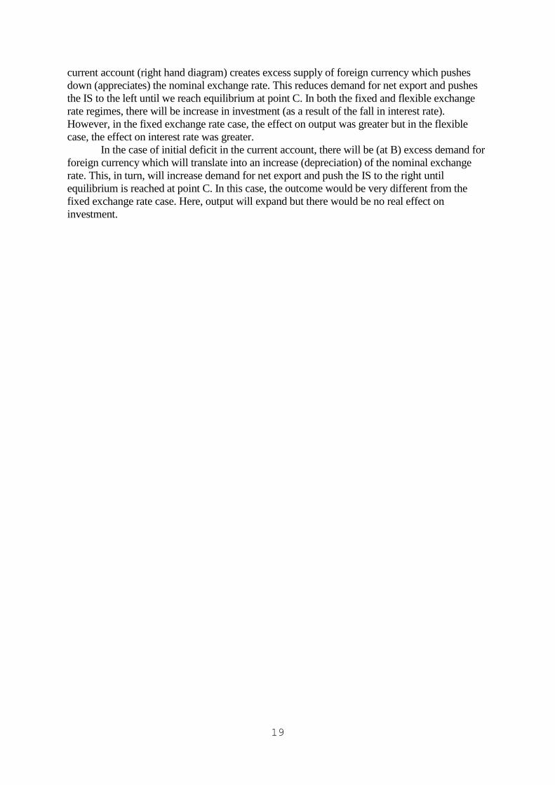
(b) Flexible exchange rate

The initial move from A to be is the same as before. This time, however, the surplus in the

YA

YB

0r

)*

(0

0

p

pEIS

),( 00 PMLM

0r

0y

),( 01 PMLM

AA

1r B

1y

B

Initial Surplus in NXInitial Deficit in NX

)*

(0

0

p

pEIS

),( 01 PMLM

),( 00 PMLM

0y 1y

C

)*

(0

1

p

pEIS

C2r

)*

(0

1

p

pEIS

19

current account (right hand diagram) creates excess supply of foreign currency which pushes

down (appreciates) the nominal exchange rate. This reduces demand for net export and pushes

the IS to the left until we reach equilibrium at point C. In both the fixed and flexible exchange

rate regimes, there will be increase in investment (as a result of the fall in interest rate).

However, in the fixed exchange rate case, the effect on output was greater but in the flexible

case, the effect on interest rate was greater.

In the case of initial deficit in the current account, there will be (at B) excess demand for

foreign currency which will translate into an increase (depreciation) of the nominal exchange

rate. This, in turn, will increase demand for net export and push the IS to the right until

equilibrium is reached at point C. In this case, the outcome would be very different from the

fixed exchange rate case. Here, output will expand but there would be no real effect on

investment.