solutions to chapter 10 problems - uitsweb.uconn.edu/tripathi/412/chap10-sol.pdf · solutions to...
TRANSCRIPT

SOLUTIONS TO CHAPTER 10 PROBLEMS
10.1. a. Since investment is likely to be affected by macroeconomic factors,
it is important to allow for these by including separate time intercepts; this
is done by using T - 1 time period dummies.
b. Putting the unobserved effect c in the equation is a simple way toi
account for time-constant features of a county that affect investment and
might also be correlated with the tax variable. Something like "average"
county economic climate, which affects investment, could easily be correlated
with tax rates because tax rates are, at least to a certain extent, selected
by state and local officials. If only a cross section were available, we
would have to find an instrument for the tax variable that is uncorrelated
with c and correlated with the tax rate. This is often a difficult task.i
c. Standard investment theories suggest that, ceteris paribus, larger
marginal tax rates decrease investment.
d. I would start with a fixed effects analysis to allow arbitrary
correlation between all time-varying explanatory variables and c . (Actually,i
doing pooled OLS is a useful initial exercise; these results can be compared
with those from an FE analysis). Such an analysis assumes strict exogeneity
of z , tax , and disaster in the sense that these are uncorrelated withit it it
the errors u for all t and s.is
I have no strong intuition for the likely serial correlation properties
of the {u }. These might have little serial correlation because we haveit
allowed for c , in which case I would use standard fixed effects. However, iti
seems more likely that the u are positively autocorrelated, in which case Iit
might use first differencing instead. In either case, I would compute the
109

fully robust standard errors along with the usual ones. Remember, with first-
differencing it is easy to test whether the changes Du are seriallyit
uncorrelated.
e. If tax and disaster do not have lagged effects on investment, thenit it
the only possible violation of the strict exogeneity assumption is if future
values of these variables are correlated with u . It is safe to say thatit
this is not a worry for the disaster variable: presumably, future natural
disasters are not determined by past investment. On the other hand, state
officials might look at the levels of past investment in determining future
tax policy, especially if there is a target level of tax revenue the officials
are are trying to achieve. This could be similar to setting property tax
rates: sometimes property tax rates are set depending on recent housing
values, since a larger base means a smaller rate can achieve the same amount
of revenue. Given that we allow tax to be correlated with c , this mightit i
not be much of a problem. But it cannot be ruled out ahead of time.
10.2. a. q , d , and G can be consistently estimated (assuming all elements of2 2
z are time-varying). The first period intercept, q , and the coefficient onit 1
female , d , cannot be estimated.i 1
b. Everything else equal, q measures the growth in wage for men over the2
period. This is because, if we set female = 0 and z = z , the change ini i1 i2
log wage is, on average, q (d2 = 0 and d2 = 1). We can think of this as2 1 2
being the growth in wage rates (for males) due to aggregate factors in the
economy. The parameter d measures the difference in wage growth rates2
between women and men, all else equal. If d = 0 then, for men and women with2
the same characteristics, average wage growth is the same.
110

c. Write
log(wage ) = q + z G + d female + c + ui1 1 i1 1 i i i1
log(wage ) = q + q + z G + d female + d female + c + u ,i2 1 2 i2 1 i 2 i i2
where I have used the fact that d2 = 0 and d2 = 1. Subtracting the first of1 2
these from the second gives
Dlog(wage ) = q + Dz G + d female + Du .i 2 i 2 i i
This equation shows explicitly that the growth in wages depends on Dz andi
gender. If z = z then Dz = 0, and the growth in wage for men is q andi1 i2 i 2
that for women is q + d , just as above. This shows that we can allow for c2 2 i
and still test for a gender differential in the growth of wages. But we
cannot say anything about the wage differential between men and women for a
given year.
----- ----- -----¨10.3. a. Let x = (x + x )/2, y = (y + y )/2, x = x - x ,i i1 i2 i i1 i2 i1 i1 i
-----¨ ¨ ¨x = x - x , and similarly for y and y . For T = 2 the fixed effectsi2 i2 i i1 i2
estimator can be written as
-1N N^ & * & *¨ ¨ ¨ ¨ ¨ ¨ ¨ ¨B = S (x’ x + x’ x ) S (x’ y + x’ y ) .FE i1 i1 i2 i2 i1 i1 i2 i27 8 7 8i=1 i=1
Now, by simple algebra,
x = (x - x )/2 = -Dx /2i1 i1 i2 i
x = (x - x )/2 = Dx /2i2 i2 i1 i
y = (y - y )/2 = -Dy /2i1 i1 i2 i
y = (y - y )/2 = Dy /2.i2 i2 i1 i
Therefore,
¨ ¨ ¨ ¨x’ x + x’ x = Dx’Dx /4 + Dx’Dx /4 = Dx’Dx /2i1 i1 i2 i2 i i i i i i
¨ ¨ ¨ ¨x’ y + x’ y = Dx’Dy /4 + Dx’Dy /4 = Dx’Dy /2,i1 i1 i2 i2 i i i i i i
111

and so
-1N N^ & * & *B = S Dx’Dx /2 S Dx’Dy /2FE i i i i7 8 7 8i=1 i=1
-1N N& * & * ^= S Dx’Dx S Dx’Dy = B .i i i i FD7 8 7 8i=1 i=1
^ ^ ^ ^¨ ¨ ¨ ¨b. Let u = y - x B and u = y - x B be the fixed effectsi1 i1 i1 FE i2 i2 i2 FE
^residuals for the two time periods for cross section observation i. Since BFE
^= B , and using the representations in (4.1’), we haveFD
^ ^ ^ ^u = -Dy /2 - (-Dx /2)B = -(Dy - Dx B )/2 _ -e /2i1 i i FD i i FD i
^ ^ ^ ^u = Dy /2 - (Dx /2)B = (Dy - Dx B )/2 _ e /2,i2 i i FD i i FD i
^ ^where e _ Dy - Dx B are the first difference residuals, i = 1,2,...,N.i i i FD
Therefore,
N N^2 ^2 ^2S (u + u ) = (1/2) S e .i1 i2 ii=1 i=1
This shows that the sum of squared residuals from the fixed effects regression
is exactly one have the sum of squared residuals from the first difference
regression. Since we know the variance estimate for fixed effects is the SSR
divided by N - K (when T = 2), and the variance estimate for first difference
is the SSR divided by N - K, the error variance from fixed effects is always
half the size as the error variance for first difference estimation, that is,
^2 ^2s = s /2 (contrary to what the problem asks you so show). What I wanted youu e
^ ^to show is that the variance matrix estimates of B and B are identical.FE FD
This is easy since the variance matrix estimate for fixed effects is
-1 -1 -1N N N^2& * ^2 & * ^2& *¨ ¨ ¨ ¨s S (x’ x + x’ x ) = (s /2) S Dx’Dx /2 = s S Dx’Dx ,u i1 i1 i2 i2 e i i e i i7 8 7 8 7 8i=1 i=1 i=1
which is the variance matrix estimator for first difference. Thus, the
standard errors, and in fact all other test statistics (F statistics) will be
numerically identical using the two approaches.
112

10.4. a. Including the aggregate time effect, d2 , can be very important.t
Without it, we must assume that any change in average y over the two time
periods is due to the program, and not to external, secular factors. For
example, if y is the unemployment rate for city i at time t, and progit it
denotes a job creation program, we want to be sure that we account for the
fact that the general economy may have worsened or improved over the period.
If d2 is omitted, and q < 0 (an improving economy, since unemployment hast 2
fallen), we might attribute a decrease in unemployment to the job creation
program, when in fact it had nothing to do with it. For general T, each time
period should have its own intercept (otherwise the analysis is not entirely
convincing).
b. The presence of c allows program participation to be correlated withi
unobserved individual heterogeneity. This is crucial in contexts where the
experimental group is not randomly assigned. Two examples are when
individuals "self-select" into the program and when program administrators
target a specific group that the program is intended to help.
c. If we first difference the equation, use the fact that prog = 0 fori1
all i, d2 = 0, and d2 = 1, we get1 2
y - y = q + d prog + u - u ,i2 i1 2 1 i2 i2 i1
or
Dy = q + d prog + Du .i 2 1 i2 i
Now, the FE (and FD) estimates of q and d are just the OLS estimators from2 1
the this equation (on cross section data). From basic two-variable regression
^with a dummy independent variable, q is the average value of Dy over the2
^ ^group with prog = 0, that is, the control group. Also, q + d is thei2 2 1
113
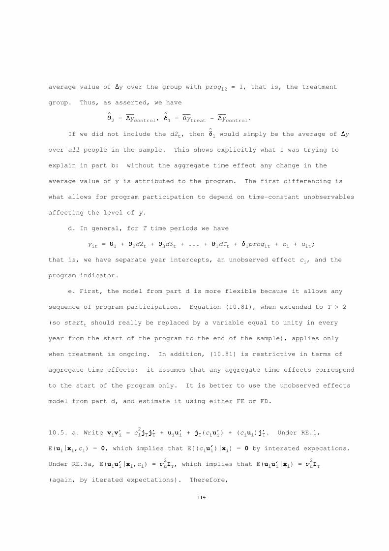
average value of Dy over the group with prog = 1, that is, the treatmenti2
group. Thus, as asserted, we have
^ ---------- ^ ---------- ----------q = Dy , d = Dy - Dy .2 control 1 treat control
^If we did not include the d2 , then d would simply be the average of Dyt 1
over all people in the sample. This shows explicitly what I was trying to
explain in part b: without the aggregate time effect any change in the
average value of y is attributed to the program. The first differencing is
what allows for program participation to depend on time-constant unobservables
affecting the level of y.
d. In general, for T time periods we have
y = q + q d2 + q d3 + ... + q dT + d prog + c + u ;it 1 2 t 3 t T t 1 it i it
that is, we have separate year intercepts, an unobserved effect c , and thei
program indicator.
e. First, the model from part d is more flexible because it allows any
sequence of program participation. Equation (10.81), when extended to T > 2
(so start should really be replaced by a variable equal to unity in everyt
year from the start of the program to the end of the sample), applies only
when treatment is ongoing. In addition, (10.81) is restrictive in terms of
aggregate time effects: it assumes that any aggregate time effects correspond
to the start of the program only. It is better to use the unobserved effects
model from part d, and estimate it using either FE or FD.
210.5. a. Write v v’ = c j j’ + u u’ + j (c u’) + (c u )j’. Under RE.1,i i i T T i i T i i i i T
E(u |x ,c ) = 0, which implies that E[(c u’)|x ) = 0 by interated expecations.i i i i i i
2 2Under RE.3a, E(u u’|x ,c ) = s I , which implies that E(u u’|x ) = s Ii i i i u T i i i u T
(again, by iterated expectations). Therefore,
114

2 2E(v v’|x ) = E(c |x )j j’ + E(u u’|x ) = h(x )j j’ + s I ,i i i i i T T i i i i T T u T
2where h(x ) _ Var(c |x ) = E(c |x ) (by RE.1b). This shows that thei i i i i
conditional variance matrix of v given x has the same covariance for all t $i i
2s, h(x ), and the same variance for all t, h(x ) + s . Therefore, while thei i u
variances and covariances depend on x in general, they do not depend on timei
separately.
-----b. The RE estimator is still consistent and rN-asymptotically normal
without assumption RE.3b, but the usual random effects variance estimator of
^B is no longer valid because E(v v’|x ) does not have the form (10.30)RE i i i
(because it depends on x ). The robust variance matrix estimator given ini
(7.49) should be used in obtaining standard errors or Wald statistics.
10.6. a. By stacking the formulas for the FD and FE estimators, and using
standard asymptotic arguments, we have, under FE.1 and the rank conditions,
N----- ^ -1& -1 *rN(Q - Q) = G N S s + o (1),i p7 8i=1
where G is the 2K * 2K block diagonal matrix with blocks A and A ,1 2
respectively, and s is the 2K * 1 vectori
& *DX’Dui is _ 2 2.i ¨ ¨X’u7 i i 8
^ ^b. Let Du denote the (T - 1) * 1 vector of FD residuals, and let ui i
denote the T * 1 vector of FE residuals. Plugging these into the formula for
N^ ^ -1 ^ ^ ^s givens s . Let D = N S s s’, and define G by replacing A and A withi i i i 1 2
i=1
^ ----- ^ ^-1^^-1their obvious consistent estimators. Then Avar[rN(Q - Q)] = G DG is a
----- ^consistent estimator of Avar rN(Q - Q).
115

c. Let R be the K * 2K partitioned matrix R = [I | -I ]. Then the nullK K
hypothesis imposed by the Hausman test is H : RQ = 0. So we can form a Wald-0
type statistic,
^ ^-1^^-1 -1 ^H = (RQ)’[RG DG R’] (RQ).
2Under FE.1 and the rank conditions for FD and FE, H has a limiting cK
distribution. The statistic requires no particular second moment assumptions
^ ^ ^of the kind in FE.3. Note that RQ = B - B .FD FE
10.7. I provide annotated Stata output, and I compute the nonrobust
regression-based statistic from equation (11.79):
. * random effects estimation
. iis id
. tis term
. xtreg trmgpa spring crsgpa frstsem season sat verbmath hsperc hssize black
female, re
Random-effects GLS regression
sd(u_id) = .3718544 Number of obs = 732
sd(e_id_t) = .4088283 n = 366
sd(e_id_t + u_id) = .5526448 T = 2
corr(u_id, X) = 0 (assumed) R-sq within = 0.2067
between = 0.5390
overall = 0.4785
chi2( 10) = 512.77
(theta = 0.3862) Prob > chi2 = 0.0000
------------------------------------------------------------------------------
trmgpa | Coef. Std. Err. z P>|z| [95% Conf. Interval]
---------+--------------------------------------------------------------------
spring | -.0606536 .0371605 -1.632 0.103 -.1334868 .0121797
crsgpa | 1.082365 .0930877 11.627 0.000 .8999166 1.264814
frstsem | .0029948 .0599542 0.050 0.960 -.1145132 .1205028
season | -.0440992 .0392381 -1.124 0.261 -.1210044 .0328061
sat | .0017052 .0001771 9.630 0.000 .0013582 .0020523
116

verbmath | -.1575199 .16351 -0.963 0.335 -.4779937 .1629538
hsperc | -.0084622 .0012426 -6.810 0.000 -.0108977 -.0060268
hssize | -.0000775 .0001248 -0.621 0.534 -.000322 .000167
black | -.2348189 .0681573 -3.445 0.000 -.3684048 -.1012331
female | .3581529 .0612948 5.843 0.000 .2380173 .4782886
_cons | -1.73492 .3566599 -4.864 0.000 -2.43396 -1.035879
------------------------------------------------------------------------------
. * fixed effects estimation, with time-varying variables only.
. xtreg trmgpa spring crsgpa frstsem season, fe
Fixed-effects (within) regression
sd(u_id) = .679133 Number of obs = 732
sd(e_id_t) = .4088283 n = 366
sd(e_id_t + u_id) = .792693 T = 2
corr(u_id, Xb) = -0.0893 R-sq within = 0.2069
between = 0.0333
overall = 0.0613
F( 4, 362) = 23.61
Prob > F = 0.0000
------------------------------------------------------------------------------
trmgpa | Coef. Std. Err. t P>|t| [95% Conf. Interval]
---------+--------------------------------------------------------------------
spring | -.0657817 .0391404 -1.681 0.094 -.1427528 .0111895
crsgpa | 1.140688 .1186538 9.614 0.000 .9073506 1.374025
frstsem | .0128523 .0688364 0.187 0.852 -.1225172 .1482218
season | -.0566454 .0414748 -1.366 0.173 -.1382072 .0249165
_cons | -.7708056 .3305004 -2.332 0.020 -1.420747 -.1208637
------------------------------------------------------------------------------
id | F(365,362) = 5.399 0.000 (366 categories)
. * Obtaining the regression-based Hausman test is a bit tedious. First,
compute the time-averages for all of the time-varying variables:
. egen atrmgpa = mean(trmgpa), by(id)
. egen aspring = mean(spring), by(id)
. egen acrsgpa = mean(crsgpa), by(id)
. egen afrstsem = mean(frstsem), by(id)
. egen aseason = mean(season), by(id)
. * Now obtain GLS transformations for both time-constant and
. * time-varying variables. Note that lamdahat = .386.
117

. di 1 - .386
.614
. gen bone = .614
. gen bsat = .614*sat
. gen bvrbmth = .614*verbmath
. gen bhsperc = .614*hsperc
. gen bhssize = .614*hssize
. gen bblack = .614*black
. gen bfemale = .614*female
. gen btrmgpa = trmgpa - .386*atrmgpa
. gen bspring = spring - .386*aspring
. gen bcrsgpa = crsgpa - .386*acrsgpa
. gen bfrstsem = frstsem - .386*afrstsem
. gen bseason = season - .386*aseason
. * Check to make sure that pooled OLS on transformed data is random
. * effects.
. reg btrmgpa bone bspring bcrsgpa bfrstsem bseason bsat bvrbmth bhsperc
bhssize bblack bfemale, nocons
Source | SS df MS Number of obs = 732
---------+------------------------------ F( 11, 721) = 862.67
Model | 1584.10163 11 144.009239 Prob > F = 0.0000
Residual | 120.359125 721 .1669336 R-squared = 0.9294
---------+------------------------------ Adj R-squared = 0.9283
Total | 1704.46076 732 2.3284983 Root MSE = .40858
------------------------------------------------------------------------------
btrmgpa | Coef. Std. Err. t P>|t| [95% Conf. Interval]
---------+--------------------------------------------------------------------
bone | -1.734843 .3566396 -4.864 0.000 -2.435019 -1.034666
bspring | -.060651 .0371666 -1.632 0.103 -.1336187 .0123167
bcrsgpa | 1.082336 .0930923 11.626 0.000 .8995719 1.265101
bfrstsem | .0029868 .0599604 0.050 0.960 -.114731 .1207046
bseason | -.0440905 .0392441 -1.123 0.262 -.1211368 .0329558
bsat | .0017052 .000177 9.632 0.000 .0013577 .0020528
bvrbmth | -.1575166 .1634784 -0.964 0.336 -.4784672 .163434
bhsperc | -.0084622 .0012424 -6.811 0.000 -.0109013 -.0060231
bhssize | -.0000775 .0001247 -0.621 0.535 -.0003224 .0001674
118

bblack | -.2348204 .0681441 -3.446 0.000 -.3686049 -.1010359
bfemale | .3581524 .0612839 5.844 0.000 .2378363 .4784686
------------------------------------------------------------------------------
. * These are the RE estimates, subject to rounding error.
. * Now add the time averages of the variables that change across i and t
. * to perform the Hausman test:
. reg btrmgpa bone bspring bcrsgpa bfrstsem bseason bsat bvrbmth bhsperc
bhssize bblack bfemale acrsgpa afrstsem aseason, nocons
Source | SS df MS Number of obs = 732
---------+------------------------------ F( 14, 718) = 676.85
Model | 1584.40773 14 113.171981 Prob > F = 0.0000
Residual | 120.053023 718 .167204767 R-squared = 0.9296
---------+------------------------------ Adj R-squared = 0.9282
Total | 1704.46076 732 2.3284983 Root MSE = .40891
------------------------------------------------------------------------------
btrmgpa | Coef. Std. Err. t P>|t| [95% Conf. Interval]
---------+--------------------------------------------------------------------
bone | -1.423761 .5182286 -2.747 0.006 -2.441186 -.4063367
bspring | -.0657817 .0391479 -1.680 0.093 -.1426398 .0110764
bcrsgpa | 1.140688 .1186766 9.612 0.000 .9076934 1.373683
bfrstsem | .0128523 .0688496 0.187 0.852 -.1223184 .148023
bseason | -.0566454 .0414828 -1.366 0.173 -.1380874 .0247967
bsat | .0016681 .0001804 9.247 0.000 .001314 .0020223
bvrbmth | -.1316462 .1654425 -0.796 0.426 -.4564551 .1931626
bhsperc | -.0084655 .0012551 -6.745 0.000 -.0109296 -.0060013
bhssize | -.0000783 .0001249 -0.627 0.531 -.0003236 .000167
bblack | -.2447934 .0685972 -3.569 0.000 -.3794684 -.1101184
bfemale | .3357016 .0711669 4.717 0.000 .1959815 .4754216
acrsgpa | -.1142992 .1234835 -0.926 0.355 -.3567312 .1281327
afrstsem | -.0480418 .0896965 -0.536 0.592 -.2241405 .1280569
aseason | .0763206 .0794119 0.961 0.337 -.0795867 .2322278
------------------------------------------------------------------------------
. test acrsgpa afrstsem aseason
( 1) acrsgpa = 0.0
( 2) afrstsem = 0.0
( 3) aseason = 0.0
F( 3, 718) = 0.61
Prob > F = 0.6085
. * Thus, we fail to reject the random effects assumptions even at very large
. * significance levels.
119

For comparison, the usual form of the Hausman test, which includes spring
2among the coefficients tested, gives p-value = .770, based on a c4
distribution (using Stata 7.0). It would have been easy to make the
regression-based test robust to any violation of RE.3: add ", robust
cluster(id)" to the regression command.
10.8. Here is my annotated Stata output, except for the heteroskedasticity-
robust standard errors asked for in part b. (Nothing much changes; in fact,
the standard errors actually get smaller.)
. * estimate by pooled OLS
. reg lcrime d78 clrprc1 clrprc2
Source | SS df MS Number of obs = 106
---------+------------------------------ F( 3, 102) = 30.27
Model | 18.7948264 3 6.26494214 Prob > F = 0.0000
Residual | 21.1114968 102 .206975459 R-squared = 0.4710
---------+------------------------------ Adj R-squared = 0.4554
Total | 39.9063233 105 .380060222 Root MSE = .45495
------------------------------------------------------------------------------
lcrime | Coef. Std. Err. t P>|t| [95% Conf. Interval]
---------+--------------------------------------------------------------------
d78 | -.0547246 .0944947 -0.579 0.564 -.2421544 .1327051
clrprc1 | -.0184955 .0053035 -3.487 0.000 -.0290149 -.007976
clrprc2 | -.0173881 .0054376 -3.198 0.002 -.0281735 -.0066026
_cons | 4.18122 .1878879 22.254 0.000 3.808545 4.553894
------------------------------------------------------------------------------
. * Test for serial correlation under strict exogeneity
. predict vhat, resid
. gen vhat_1 = vhat[_n-1] if d78
(53 missing values generated)
. reg vhat vhat_1
Source | SS df MS Number of obs = 53
---------+------------------------------ F( 1, 51) = 33.85
Model | 3.8092697 1 3.8092697 Prob > F = 0.0000
Residual | 5.73894345 51 .112528303 R-squared = 0.3990
120

---------+------------------------------ Adj R-squared = 0.3872
Total | 9.54821315 52 .183619484 Root MSE = .33545
------------------------------------------------------------------------------
vhat | Coef. Std. Err. t P>|t| [95% Conf. Interval]
---------+--------------------------------------------------------------------
vhat_1 | .5739582 .0986485 5.818 0.000 .3759132 .7720032
_cons | -3.01e-09 .0460779 -0.000 1.000 -.0925053 .0925053
------------------------------------------------------------------------------
. * Strong evidence of positive serial correlation in the composite error.
. * Now use first differences, as this is the same as FE:
. reg clcrime cclrprc1 cclrprc2
Source | SS df MS Number of obs = 53
---------+------------------------------ F( 2, 50) = 5.99
Model | 1.42294697 2 .711473484 Prob > F = 0.0046
Residual | 5.93723904 50 .118744781 R-squared = 0.1933
---------+------------------------------ Adj R-squared = 0.1611
Total | 7.36018601 52 .141542039 Root MSE = .34459
------------------------------------------------------------------------------
clcrime | Coef. Std. Err. t P>|t| [95% Conf. Interval]
---------+--------------------------------------------------------------------
cclrprc1 | -.0040475 .0047199 -0.858 0.395 -.0135276 .0054326
cclrprc2 | -.0131966 .0051946 -2.540 0.014 -.0236302 -.0027629
_cons | .0856556 .0637825 1.343 0.185 -.0424553 .2137665
------------------------------------------------------------------------------
At this point, we should discuss how to test H : b = b . One way to0 1 2
proceed is as follows. Write q = b - b , so that the null can be written as1 1 2
H : q = 0. Now substitute b = q + b into0 1 1 1 2
Dlcrime = b + b Dclrprc + b Dclrprc + Du0 1 -1 2 -2
to get
Dlcrime = b + q Dclrprc + b (Dclrprc + Dclrprc ) + Du.0 1 -1 2 -1 -2
Thus, we regress Dlcrime on Dclrprc and Dclrprc + Dclrprc and test the-1 -1 -2
coefficient on Dclrprc :-1
. gen cclrprcs = cclrprc1 + cclrprc2
(53 missing values generated)
. reg clcrime cclrprc1 cclrprcs
121

Source | SS df MS Number of obs = 53
---------+------------------------------ F( 2, 50) = 5.99
Model | 1.42294697 2 .711473484 Prob > F = 0.0046
Residual | 5.93723904 50 .118744781 R-squared = 0.1933
---------+------------------------------ Adj R-squared = 0.1611
Total | 7.36018601 52 .141542039 Root MSE = .34459
------------------------------------------------------------------------------
clcrime | Coef. Std. Err. t P>|t| [95% Conf. Interval]
---------+--------------------------------------------------------------------
cclrprc1 | .009149 .0085216 1.074 0.288 -.007967 .0262651
cclrprcs | -.0131966 .0051946 -2.540 0.014 -.0236302 -.0027629
_cons | .0856556 .0637825 1.343 0.185 -.0424553 .2137665
------------------------------------------------------------------------------
. * We fail to reject the null, so we might average the clearup percentage
. * over the past two years and then difference:
. reg clcrime cavgclr
Source | SS df MS Number of obs = 53
---------+------------------------------ F( 1, 51) = 10.80
Model | 1.28607105 1 1.28607105 Prob > F = 0.0018
Residual | 6.07411496 51 .119100293 R-squared = 0.1747
---------+------------------------------ Adj R-squared = 0.1586
Total | 7.36018601 52 .141542039 Root MSE = .34511
------------------------------------------------------------------------------
clcrime | Coef. Std. Err. t P>|t| [95% Conf. Interval]
---------+--------------------------------------------------------------------
cavgclr | -.0166511 .0050672 -3.286 0.002 -.0268239 -.0064783
_cons | .0993289 .0625916 1.587 0.119 -.0263289 .2249867
------------------------------------------------------------------------------
. * Now the effect is very significant, and the goodness-of-fit does not
. * suffer very much.
10.9. a. One simple way to compute a Hausman test is to just add the time
averages of all explanatory variables, excluding the dummy variables, and
estimating the equation by random effects. I should have done a better job of
spelling this out in the text. In other words, write
-----y = x B + w X + r , t = 1,...,T,it it i it
122

where x includes an overall intercept along with time dummies, as well asit
w , the covariates that change across i and t. We can estimate this equationit
by random effects and test H : X = 0. Conveniently, we can use this0
formulation to compute a test that is fully robust to violations of RE.3. The
Stata session follows. The "xtgee" command is needed to obtain the robust
test. (The generalized estimating equation approach in the linear random
effects context is iterated random effects estimation. In the example here,
it iterates only once.)
. xtreg lcrmrte lprbarr lprbconv lprbpris lavgsen lpolpc d82-d87, fe
Fixed-effects (within) regression Number of obs = 630
Group variable (i) : county Number of groups = 90
R-sq: within = 0.4342 Obs per group: min = 7
between = 0.4066 avg = 7.0
overall = 0.4042 max = 7
F(11,529) = 36.91
corr(u_i, Xb) = 0.2068 Prob > F = 0.0000
------------------------------------------------------------------------------
lcrmrte | Coef. Std. Err. t P>|t| [95% Conf. Interval]
-------------+----------------------------------------------------------------
lprbarr | -.3597944 .0324192 -11.10 0.000 -.4234806 -.2961083
lprbconv | -.2858733 .0212173 -13.47 0.000 -.3275538 -.2441928
lprbpris | -.1827812 .0324611 -5.63 0.000 -.2465496 -.1190127
lavgsen | -.0044879 .0264471 -0.17 0.865 -.0564421 .0474663
lpolpc | .4241142 .0263661 16.09 0.000 .3723191 .4759093
d82 | .0125802 .0215416 0.58 0.559 -.0297373 .0548977
d83 | -.0792813 .0213399 -3.72 0.000 -.1212027 -.0373598
d84 | -.1177281 .0216145 -5.45 0.000 -.1601888 -.0752673
d85 | -.1119561 .0218459 -5.12 0.000 -.1548715 -.0690407
d86 | -.0818268 .0214266 -3.82 0.000 -.1239185 -.0397352
d87 | -.0404704 .0210392 -1.92 0.055 -.0818011 .0008602
_cons | -1.604135 .1685739 -9.52 0.000 -1.935292 -1.272979
-------------+----------------------------------------------------------------
sigma_u | .43487416
sigma_e | .13871215
rho | .90765322 (fraction of variance due to u_i)
------------------------------------------------------------------------------
F test that all u_i=0: F(89, 529) = 45.87 Prob > F = 0.0000
123

. xtreg lcrmrte lprbarr lprbconv lprbpris lavgsen lpolpc d82-d87, re
Random-effects GLS regression Number of obs = 630
Group variable (i) : county Number of groups = 90
R-sq: within = 0.4287 Obs per group: min = 7
between = 0.4533 avg = 7.0
overall = 0.4454 max = 7
Random effects u_i ~ Gaussian Wald chi2(11) = 459.17
corr(u_i, X) = 0 (assumed) Prob > chi2 = 0.0000
------------------------------------------------------------------------------
lcrmrte | Coef. Std. Err. z P>|z| [95% Conf. Interval]
-------------+----------------------------------------------------------------
lprbarr | -.4252097 .0318705 -13.34 0.000 -.4876748 -.3627447
lprbconv | -.3271464 .0209708 -15.60 0.000 -.3682485 -.2860443
lprbpris | -.1793507 .0339945 -5.28 0.000 -.2459788 -.1127226
lavgsen | -.0083696 .0279544 -0.30 0.765 -.0631592 .0464201
lpolpc | .4294148 .0261488 16.42 0.000 .378164 .4806655
d82 | .0137442 .022943 0.60 0.549 -.0312232 .0587117
d83 | -.075388 .0227367 -3.32 0.001 -.1199511 -.0308249
d84 | -.1130975 .0230083 -4.92 0.000 -.158193 -.068002
d85 | -.1057261 .0232488 -4.55 0.000 -.1512928 -.0601593
d86 | -.0795307 .0228326 -3.48 0.000 -.1242817 -.0347796
d87 | -.0424581 .0223994 -1.90 0.058 -.0863601 .001444
_cons | -1.672632 .1749952 -9.56 0.000 -2.015617 -1.329648
-------------+----------------------------------------------------------------
sigma_u | .30032934
sigma_e | .13871215
rho | .82418424 (fraction of variance due to u_i)
------------------------------------------------------------------------------
. xthausman
Hausman specification test
---- Coefficients ----
| Fixed Random
lcrmrte | Effects Effects Difference
-------------+-----------------------------------------
lprbarr | -.3597944 -.4252097 .0654153
lprbconv | -.2858733 -.3271464 .0412731
lprbpris | -.1827812 -.1793507 -.0034305
lavgsen | -.0044879 -.0083696 .0038816
lpolpc | .4241142 .4294148 -.0053005
d82 | .0125802 .0137442 -.001164
d83 | -.0792813 -.075388 -.0038933
d84 | -.1177281 -.1130975 -.0046306
d85 | -.1119561 -.1057261 -.00623
d86 | -.0818268 -.0795307 -.0022962
d87 | -.0404704 -.0424581 .0019876
124

Test: Ho: difference in coefficients not systematic
chi2( 11) = (b-B)’[S^(-1)](b-B), S = (S_fe - S_re)
= 121.31
Prob>chi2 = 0.0000
. * This version of the Hausman test reports too many degrees-of-freedom.
. * It turns out that there are degeneracies in the asymptotic variance
. * of the Hausman statistic. This problem is easily overcome by only
. * testing the coefficients on the non-year dummies. To do this, we
. * compute the time averages for the explanatory variables, excluding
. * the time dummies.
. egen lprbata = mean(lprbarr), by(county)
. egen lprbcta = mean(lprbconv), by(county)
. egen lprbpta = mean(lprbpris), by(county)
. egen lavgta = mean(lavgsen), by(county)
. egen lpolta = mean(lpolpc), by(county)
. xtreg lcrmrte lprbarr lprbconv lprbpris lavgsen lpolpc d82-d87 lprbata-
lpolta, re
Random-effects GLS regression Number of obs = 630
Group variable (i) : county Number of groups = 90
R-sq: within = 0.4342 Obs per group: min = 7
between = 0.7099 avg = 7.0
overall = 0.6859 max = 7
Random effects u_i ~ Gaussian Wald chi2(16) = 611.57
corr(u_i, X) = 0 (assumed) Prob > chi2 = 0.0000
------------------------------------------------------------------------------
lcrmrte | Coef. Std. Err. z P>|z| [95% Conf. Interval]
-------------+----------------------------------------------------------------
lprbarr | -.3597944 .0324192 -11.10 0.000 -.4233349 -.296254
lprbconv | -.2858733 .0212173 -13.47 0.000 -.3274584 -.2442881
lprbpris | -.1827812 .0324611 -5.63 0.000 -.2464037 -.1191586
lavgsen | -.0044879 .0264471 -0.17 0.865 -.0563232 .0473474
lpolpc | .4241142 .0263661 16.09 0.000 .3724376 .4757908
d82 | .0125802 .0215416 0.58 0.559 -.0296405 .0548009
d83 | -.0792813 .0213399 -3.72 0.000 -.1211068 -.0374557
d84 | -.1177281 .0216145 -5.45 0.000 -.1600917 -.0753645
d85 | -.1119561 .0218459 -5.12 0.000 -.1547734 -.0691389
d86 | -.0818268 .0214266 -3.82 0.000 -.1238222 -.0398315
d87 | -.0404704 .0210392 -1.92 0.054 -.0817065 .0007657
lprbata | -.4530581 .0980908 -4.62 0.000 -.6453126 -.2608036
125

lprbcta | -.3061992 .073276 -4.18 0.000 -.4498175 -.1625808
lprbpta | 1.343451 .2397992 5.60 0.000 .8734534 1.813449
lavgta | -.126782 .210188 -0.60 0.546 -.5387428 .2851789
lpolta | -.0794158 .0763314 -1.04 0.298 -.2290227 .070191
_cons | -1.455678 .7064912 -2.06 0.039 -2.840375 -.0709804
-------------+----------------------------------------------------------------
sigma_u | .30032934
sigma_e | .13871215
rho | .82418424 (fraction of variance due to u_i)
------------------------------------------------------------------------------
. testparm lprbata-lpolta
( 1) lprbata = 0.0
( 2) lprbcta = 0.0
( 3) lprbpta = 0.0
( 4) lavgta = 0.0
( 5) lpolta = 0.0
chi2( 5) = 89.57
Prob > chi2 = 0.0000
. * This is a strong statistical rejection that the plims of fixed effects
. * and random effects are the same. Note that the estimates on the
. * original variables are simply the fixed effects estimates, including
. * those on the time dummies.
. * The above test maintains RE.3 in addition to RE.1. The following gives
. * a test that works without RE.3:
. xtgee lcrmrte lprbarr lprbconv lprbpris lavgsen lpolpc d82-d87 lprbata-
lpolta, corr(excha) robust
Iteration 1: tolerance = 6.134e-08
GEE population-averaged model Number of obs = 630
Group variable: county Number of groups = 90
Link: identity Obs per group: min = 7
Family: Gaussian avg = 7.0
Correlation: exchangeable max = 7
Wald chi2(16) = 401.23
Scale parameter: .1029064 Prob > chi2 = 0.0000
(standard errors adjusted for clustering on county)
------------------------------------------------------------------------------
| Semi-robust
lcrmrte | Coef. Std. Err. z P>|z| [95% Conf. Interval]
-------------+----------------------------------------------------------------
lprbarr | -.3597944 .0589455 -6.10 0.000 -.4753255 -.2442633
lprbconv | -.2858733 .0510695 -5.60 0.000 -.3859677 -.1857789
lprbpris | -.1827812 .0448835 -4.07 0.000 -.2707511 -.0948112
lavgsen | -.0044879 .033057 -0.14 0.892 -.0692785 .0603027
126

lpolpc | .4241142 .0841595 5.04 0.000 .2591647 .5890638
d82 | .0125802 .015866 0.79 0.428 -.0185167 .0436771
d83 | -.0792813 .0193921 -4.09 0.000 -.1172891 -.0412734
d84 | -.1177281 .0215211 -5.47 0.000 -.1599087 -.0755474
d85 | -.1119561 .025433 -4.40 0.000 -.1618038 -.0621084
d86 | -.0818268 .0234201 -3.49 0.000 -.1277294 -.0359242
d87 | -.0404704 .0239642 -1.69 0.091 -.0874394 .0064985
lprbata | -.4530581 .1072689 -4.22 0.000 -.6633013 -.2428149
lprbcta | -.3061992 .0986122 -3.11 0.002 -.4994755 -.1129229
lprbpta | 1.343451 .2902148 4.63 0.000 .7746406 1.912262
lavgta | -.126782 .2587182 -0.49 0.624 -.6338604 .3802965
lpolta | -.0794158 .0955707 -0.83 0.406 -.2667309 .1078992
_cons | -1.455678 .8395033 -1.73 0.083 -3.101074 .1897186
------------------------------------------------------------------------------
. testparm lprbata-lpolta
( 1) lprbata = 0.0
( 2) lprbcta = 0.0
( 3) lprbpta = 0.0
( 4) lavgta = 0.0
( 5) lpolta = 0.0
chi2( 5) = 62.11
Prob > chi2 = 0.0000
. * Perhaps not surprisingly, the robust statistic is smaller, but the
. * statistical rejection is still very strong.
b. Fixed effects estimation with the nine wage variables gives:
. xtreg lcrmrte lprbarr lprbconv lprbpris lavgsen lpolpc lwcon-lwloc d82-d87,
fe
Fixed-effects (within) regression Number of obs = 630
Group variable (i) : county Number of groups = 90
R-sq: within = 0.4575 Obs per group: min = 7
between = 0.2518 avg = 7.0
overall = 0.2687 max = 7
F(20,520) = 21.92
corr(u_i, Xb) = 0.0804 Prob > F = 0.0000
------------------------------------------------------------------------------
lcrmrte | Coef. Std. Err. t P>|t| [95% Conf. Interval]
-------------+----------------------------------------------------------------
lprbarr | -.3563515 .0321591 -11.08 0.000 -.4195292 -.2931738
lprbconv | -.2859539 .0210513 -13.58 0.000 -.3273099 -.2445979
lprbpris | -.1751355 .0323403 -5.42 0.000 -.2386693 -.1116017
lavgsen | -.0028739 .0262108 -0.11 0.913 -.054366 .0486181
127

lpolpc | .4229 .0263942 16.02 0.000 .3710476 .4747524
lwcon | -.0345448 .0391616 -0.88 0.378 -.1114792 .0423896
lwtuc | .0459747 .019034 2.42 0.016 .0085817 .0833677
lwtrd | -.0201766 .0406073 -0.50 0.619 -.0999511 .0595979
lwfir | -.0035445 .028333 -0.13 0.900 -.0592058 .0521168
lwser | .0101264 .0191915 0.53 0.598 -.027576 .0478289
lwmfg | -.3005691 .1094068 -2.75 0.006 -.5155028 -.0856354
lwfed | -.3331226 .176448 -1.89 0.060 -.6797612 .013516
lwsta | .0215209 .1130648 0.19 0.849 -.2005991 .2436409
lwloc | .1810215 .1180643 1.53 0.126 -.0509202 .4129632
d82 | .0188915 .0251244 0.75 0.452 -.0304662 .0682492
d83 | -.055286 .0330287 -1.67 0.095 -.1201721 .0096001
d84 | -.0615162 .0410805 -1.50 0.135 -.1422204 .0191879
d85 | -.0397115 .0561635 -0.71 0.480 -.1500468 .0706237
d86 | -.0001133 .0680124 -0.00 0.999 -.1337262 .1334996
d87 | .0537042 .0798953 0.67 0.502 -.1032531 .2106615
_cons | .8931726 1.424067 0.63 0.531 -1.904459 3.690805
-------------+----------------------------------------------------------------
sigma_u | .47756823
sigma_e | .13700505
rho | .92395784 (fraction of variance due to u_i)
------------------------------------------------------------------------------
F test that all u_i=0: F(89, 520) = 39.12 Prob > F = 0.0000
. testparm lwcon-lwloc
( 1) lwcon = 0.0
( 2) lwtuc = 0.0
( 3) lwtrd = 0.0
( 4) lwfir = 0.0
( 5) lwser = 0.0
( 6) lwmfg = 0.0
( 7) lwfed = 0.0
( 8) lwsta = 0.0
( 9) lwloc = 0.0
F( 9, 520) = 2.47
Prob > F = 0.0090
. * Jointly, the wage variables are significant (using the version of the
. * test that maintains FE.3), but the signs in some cases are hard to
. * interpret.
c. First, we need to compute the changes in log wages. Then, we just
used pooled OLS.
. sort county year
128

. gen clwcon = lwcon - lwcon[_n-1] if year > 81
(90 missing values generated)
. gen clwtuc = lwtuc - lwtuc[_n-1] if year > 81
(90 missing values generated)
. gen clwtrd = lwtrd - lwtrd[_n-1] if year > 81
(90 missing values generated)
. gen clwfir = lwfir - lwfir[_n-1] if year > 81
(90 missing values generated)
. gen clwser = lwser - lwser[_n-1] if year > 81
(90 missing values generated)
. gen clwmfg = lwmfg - lwmfg[_n-1] if year > 81
(90 missing values generated)
. gen clwfed = lwfed - lwfed[_n-1] if year > 81
(90 missing values generated)
. gen clwsta = lwsta - lwsta[_n-1] if year > 81
(90 missing values generated)
. gen clwloc = lwloc - lwloc[_n-1] if year > 81
(90 missing values generated)
. reg clcrmrte clprbarr clprbcon clprbpri clavgsen clpolpc clwcon-clwloc d83-
d87
Source | SS df MS Number of obs = 540
-------------+------------------------------ F( 19, 520) = 21.90
Model | 9.86742162 19 .51933798 Prob > F = 0.0000
Residual | 12.3293822 520 .02371035 R-squared = 0.4445
-------------+------------------------------ Adj R-squared = 0.4242
Total | 22.1968038 539 .041181454 Root MSE = .15398
------------------------------------------------------------------------------
clcrmrte | Coef. Std. Err. t P>|t| [95% Conf. Interval]
-------------+----------------------------------------------------------------
clprbarr | -.3230993 .0300195 -10.76 0.000 -.3820737 -.2641248
clprbcon | -.2402885 .0182474 -13.17 0.000 -.2761362 -.2044407
clprbpri | -.1693859 .02617 -6.47 0.000 -.2207978 -.117974
clavgsen | -.0156167 .0224126 -0.70 0.486 -.0596469 .0284136
clpolpc | .3977221 .026987 14.74 0.000 .3447051 .450739
clwcon | -.0442368 .0304142 -1.45 0.146 -.1039865 .015513
clwtuc | .0253997 .0142093 1.79 0.074 -.002515 .0533144
clwtrd | -.0290309 .0307907 -0.94 0.346 -.0895203 .0314586
clwfir | .009122 .0212318 0.43 0.668 -.0325886 .0508326
clwser | .0219549 .0144342 1.52 0.129 -.0064016 .0503113
clwmfg | -.1402482 .1019317 -1.38 0.169 -.3404967 .0600003
clwfed | .0174221 .1716065 0.10 0.919 -.319705 .3545493
129

clwsta | -.0517891 .0957109 -0.54 0.589 -.2398166 .1362385
clwloc | -.0305153 .1021028 -0.30 0.765 -.2310999 .1700694
d83 | -.1108653 .0268105 -4.14 0.000 -.1635355 -.0581951
d84 | -.0374103 .024533 -1.52 0.128 -.0856063 .0107856
d85 | -.0005856 .024078 -0.02 0.981 -.0478877 .0467164
d86 | .0314757 .0245099 1.28 0.200 -.0166749 .0796262
d87 | .0388632 .0247819 1.57 0.117 -.0098218 .0875482
_cons | .0198522 .0206974 0.96 0.338 -.0208086 .060513
------------------------------------------------------------------------------
. * There are no notable differences between the FE and FD estimates, or
. * their standard errors.
d. The following set of commands tests the differenced errors for serial
correlation:
. predict ehat, resid
(90 missing values generated)
. gen ehat_1 = ehat[_n-1] if year > 82
(180 missing values generated)
. reg ehat ehat_1
Source | SS df MS Number of obs = 450
-------------+------------------------------ F( 1, 448) = 21.29
Model | .490534556 1 .490534556 Prob > F = 0.0000
Residual | 10.3219221 448 .023040005 R-squared = 0.0454
-------------+------------------------------ Adj R-squared = 0.0432
Total | 10.8124566 449 .024081195 Root MSE = .15179
------------------------------------------------------------------------------
ehat | Coef. Std. Err. t P>|t| [95% Conf. Interval]
-------------+----------------------------------------------------------------
ehat_1 | -.222258 .0481686 -4.61 0.000 -.3169225 -.1275936
_cons | 5.97e-10 .0071554 0.00 1.000 -.0140624 .0140624
------------------------------------------------------------------------------
. * There is evidence of negative serial correlation, which suggests that the
. * idiosyncratic errors in levels may follow a stable AR(1) process.
10.10. a. To allow for different intercepts in the original model, I simply
include a year dummy for 1993 in the FD equation. (The three years of data
are 1987, 1990, and 1993.) The Stata output follows:
130

. reg cmrdrte d93 cexec cunem
Source | SS df MS Number of obs = 102
-------------+------------------------------ F( 3, 98) = 0.84
Model | 46.7620386 3 15.5873462 Prob > F = 0.4736
Residual | 1812.28688 98 18.4927233 R-squared = 0.0252
-------------+------------------------------ Adj R-squared = -0.0047
Total | 1859.04892 101 18.406425 Root MSE = 4.3003
------------------------------------------------------------------------------
cmrdrte | Coef. Std. Err. t P>|t| [95% Conf. Interval]
-------------+----------------------------------------------------------------
d93 | -1.296717 1.016118 -1.28 0.205 -3.313171 .7197367
cexec | -.1150682 .1473871 -0.78 0.437 -.407553 .1774166
cunem | .1630854 .3079049 0.53 0.598 -.4479419 .7741127
_cons | 1.51099 .6608967 2.29 0.024 .1994623 2.822518
------------------------------------------------------------------------------
. predict ehat, resid
(51 missing values generated)
. gen ehat_1 = ehat[_n-1] if d93
(102 missing values generated)
. reg ehat ehat_1
Source | SS df MS Number of obs = 51
-------------+------------------------------ F( 1, 49) = 0.06
Model | .075953071 1 .075953071 Prob > F = 0.8016
Residual | 58.3045094 49 1.18988795 R-squared = 0.0013
-------------+------------------------------ Adj R-squared = -0.0191
Total | 58.3804625 50 1.16760925 Root MSE = 1.0908
------------------------------------------------------------------------------
ehat | Coef. Std. Err. t P>|t| [95% Conf. Interval]
-------------+----------------------------------------------------------------
ehat_1 | .0065807 .0260465 0.25 0.802 -.0457618 .0589231
_cons | -9.10e-10 .1527453 -0.00 1.000 -.3069532 .3069532
------------------------------------------------------------------------------
There is no evidence for serial correlation in the {u : t = 1,2,3}.it
b. The FE estimates are similar to the FD estimates. While executions
have an estimated negative effect, and the unemployment rate a positive
effect, neither is close to being significant at the usual significance
levels. Note that the time dummy coefficients are not comparable across
131

estimation methods. (If I wanted these to be comparable, I would difference
the time dummies in the FD esimation.)
. xtreg mrdrte d90 d93 exec unem, fe
Fixed-effects (within) regression Number of obs = 153
Group variable (i) : id Number of groups = 51
R-sq: within = 0.0734 Obs per group: min = 3
between = 0.0037 avg = 3.0
overall = 0.0108 max = 3
F(4,98) = 1.94
corr(u_i, Xb) = 0.0010 Prob > F = 0.1098
------------------------------------------------------------------------------
mrdrte | Coef. Std. Err. t P>|t| [95% Conf. Interval]
-------------+----------------------------------------------------------------
d90 | 1.556215 .7453273 2.09 0.039 .0771369 3.035293
d93 | 1.733242 .7004381 2.47 0.015 .3432454 3.123239
exec | -.1383231 .1770059 -0.78 0.436 -.4895856 .2129395
unem | .2213158 .2963756 0.75 0.457 -.366832 .8094636
_cons | 5.822104 1.915611 3.04 0.003 2.020636 9.623572
-------------+----------------------------------------------------------------
sigma_u | 8.7527226
sigma_e | 3.5214244
rho | .86068589 (fraction of variance due to u_i)
------------------------------------------------------------------------------
F test that all u_i=0: F(50, 98) = 17.18 Prob > F = 0.0000
c. The explanatory variable exec might fail strict exogeneity if statesit
increase future executions in response to current positive shocks to the
murder rate. Given only a three year window, this is perhaps unlikely, as the
judicial process in capital cases tends to move slowly. Nevertheless, with a
longer time series, we could add exec in the equation and estimate it byi,t+1
fixed effects.
10.11. a. The key coefficient is b . Since AFDC participation gives women1
access to better nutrition and prenatal care, we hope that AFDC participation
132

causes the percent of low-weight births to fall. This only makes sense, of
course, when we think about holding economic variables fixed, and controlling
for quality of other kinds of health care. My expectation was that b would2
be negative: more physicians means relatively fewer low-weight births. The
variable bedspc is another proxy for health-care availibility, and we expect
b < 0. Higher per capita income should lead to lower lowbrth (b < 0). The3 4
effect of population on a per capita variable is ambiguous, especially since
it is not a density measure.
b. The Stata output follows. Both the usual and fully robust standard
errors are computed. The standard errors robust to serial correlation (and
heteroskedasticity) are, as expected, somewhat larger. (If you test for AR(1)
serial correlation in the composite error, v , it is very strong. In fact,it
the estimated AR(1) coefficient is slightly above one.) Only the per capita
income variable is statistically significant. The estimate implies that a 10
percent rise in per capita income is associated with a .25 percentage point
fall in the percent of low-weight births.
. reg lowbrth d90 afdcprc lphypc lbedspc lpcinc lpopul
Source | SS df MS Number of obs = 100
-------------+------------------------------ F( 6, 93) = 5.19
Model | 33.7710894 6 5.6285149 Prob > F = 0.0001
Residual | 100.834005 93 1.08423661 R-squared = 0.2509
-------------+------------------------------ Adj R-squared = 0.2026
Total | 134.605095 99 1.35964742 Root MSE = 1.0413
------------------------------------------------------------------------------
lowbrth | Coef. Std. Err. t P>|t| [95% Conf. Interval]
-------------+----------------------------------------------------------------
d90 | .5797136 .2761244 2.10 0.038 .0313853 1.128042
afdcprc | .0955932 .0921802 1.04 0.302 -.0874584 .2786448
lphypc | .3080648 .71546 0.43 0.668 -1.112697 1.728827
lbedspc | .2790041 .5130275 0.54 0.588 -.7397668 1.297775
lpcinc | -2.494685 .9783021 -2.55 0.012 -4.437399 -.5519712
lpopul | .739284 .7023191 1.05 0.295 -.6553825 2.133951
133

_cons | 26.57786 7.158022 3.71 0.000 12.36344 40.79227
------------------------------------------------------------------------------
. reg lowbrth d90 afdcprc lphypc lbedspc lpcinc lpopul, robust cluster(state)
Regression with robust standard errors Number of obs = 100
F( 6, 49) = 4.73
Prob > F = 0.0007
R-squared = 0.2509
Number of clusters (state) = 50 Root MSE = 1.0413
------------------------------------------------------------------------------
| Robust
lowbrth | Coef. Std. Err. t P>|t| [95% Conf. Interval]
-------------+----------------------------------------------------------------
d90 | .5797136 .2214303 2.62 0.012 .1347327 1.024694
afdcprc | .0955932 .1199883 0.80 0.429 -.1455324 .3367188
lphypc | .3080648 .9063342 0.34 0.735 -1.513282 2.129411
lbedspc | .2790041 .7853754 0.36 0.724 -1.299267 1.857275
lpcinc | -2.494685 1.203901 -2.07 0.044 -4.914014 -.0753567
lpopul | .739284 .9041915 0.82 0.418 -1.077757 2.556325
_cons | 26.57786 9.29106 2.86 0.006 7.906773 45.24894
------------------------------------------------------------------------------
c. The FD (equivalently, FE) estimates are give below. The
heteroskedasticity-robust standard error for the AFDC variable is actually
smaller. In any case, removing the state unobserved effect changes the sign
on the AFDC participation variable, and it is marginally significant. Oddly,
physicians-per-capita now has a positive, significant effect on percent of
low-weight births. The hospital beds-per-capita variable has the expected
negative effect.
. reg clowbrth cafdcprc clphypc clbedspc clpcinc clpopul
Source | SS df MS Number of obs = 50
-------------+------------------------------ F( 5, 44) = 2.53
Model | .861531934 5 .172306387 Prob > F = 0.0428
Residual | 3.00026764 44 .068187901 R-squared = 0.2231
-------------+------------------------------ Adj R-squared = 0.1348
Total | 3.86179958 49 .078812236 Root MSE = .26113
------------------------------------------------------------------------------
clowbrth | Coef. Std. Err. t P>|t| [95% Conf. Interval]
-------------+----------------------------------------------------------------
134

cafdcprc | -.1760763 .0903733 -1.95 0.058 -.3582116 .006059
clphypc | 5.894509 2.816689 2.09 0.042 .2178453 11.57117
clbedspc | -1.576195 .8852111 -1.78 0.082 -3.36022 .2078308
clpcinc | -.8455268 1.356773 -0.62 0.536 -3.579924 1.88887
clpopul | 3.441116 2.872175 1.20 0.237 -2.347372 9.229604
_cons | .1060158 .3090664 0.34 0.733 -.5168667 .7288983
------------------------------------------------------------------------------
d. Adding a quadratic in afdcprc yields, not surprisingly, a diminishing
impact of AFDC participation. The turning point in the quadratic is at about
afdcprc = 6.3, and only four states have AFDC participation rates about 6.3
percent. So, the largest effect is at low AFDC participation rates, but the
effect is negative until afdcprc = 6.3. This seems reasonable. However, the
quadratic is not statistically significant at the usual levels.
. reg clowbrth cafdcprc cafdcpsq clphypc clbedspc clpcinc clpopul
Source | SS df MS Number of obs = 50
-------------+------------------------------ F( 6, 43) = 2.39
Model | .964889165 6 .160814861 Prob > F = 0.0444
Residual | 2.89691041 43 .06737001 R-squared = 0.2499
-------------+------------------------------ Adj R-squared = 0.1452
Total | 3.86179958 49 .078812236 Root MSE = .25956
------------------------------------------------------------------------------
clowbrth | Coef. Std. Err. t P>|t| [95% Conf. Interval]
-------------+----------------------------------------------------------------
cafdcprc | -.5035049 .2791959 -1.80 0.078 -1.066557 .0595472
cafdcpsq | .0396094 .0319788 1.24 0.222 -.0248819 .1041008
clphypc | 6.620885 2.860505 2.31 0.025 .8521271 12.38964
clbedspc | -1.407963 .8903074 -1.58 0.121 -3.203439 .3875124
clpcinc | -.9987865 1.354276 -0.74 0.465 -3.729945 1.732372
clpopul | 4.429026 2.964218 1.49 0.142 -1.54889 10.40694
_cons | .1245915 .3075731 0.41 0.687 -.4956887 .7448718
------------------------------------------------------------------------------
. di .504/(2*.040)
6.3
. sum afdcprc if d90
Variable | Obs Mean Std. Dev. Min Max
-------------+-----------------------------------------------------
afdcprc | 50 4.162976 1.317277 1.688183 7.358795
135

. count if d90 & afdcprc > 6.3
4
10.12. a. Even if c is uncorrelated with x for all t, the usual OLSi it
standard errors do not account for the serial correlation in v = c + u .it i it
You can see that the robust standard errors are substantially larger than the
usual ones, in some cases more than double.
. reg lwage educ black hisp exper expersq married union d81-d87, robust
cluster(nr)
Regression with robust standard errors Number of obs = 4360
F( 14, 544) = 47.10
Prob > F = 0.0000
R-squared = 0.1893
Number of clusters (nr) = 545 Root MSE = .48033
------------------------------------------------------------------------------
| Robust
lwage | Coef. Std. Err. t P>|t| [95% Conf. Interval]
-------------+----------------------------------------------------------------
educ | .0913498 .0110822 8.24 0.000 .0695807 .1131189
black | -.1392342 .0505238 -2.76 0.006 -.2384798 -.0399887
hisp | .0160195 .0390781 0.41 0.682 -.060743 .092782
exper | .0672345 .0195958 3.43 0.001 .0287417 .1057273
expersq | -.0024117 .0010252 -2.35 0.019 -.0044255 -.0003979
married | .1082529 .026034 4.16 0.000 .0571135 .1593924
union | .1824613 .0274435 6.65 0.000 .1285531 .2363695
d81 | .05832 .028228 2.07 0.039 .0028707 .1137693
d82 | .0627744 .0369735 1.70 0.090 -.0098538 .1354027
d83 | .0620117 .046248 1.34 0.181 -.0288348 .1528583
d84 | .0904672 .057988 1.56 0.119 -.0234406 .204375
d85 | .1092463 .0668474 1.63 0.103 -.0220644 .240557
d86 | .1419596 .0762348 1.86 0.063 -.007791 .2917102
d87 | .1738334 .0852056 2.04 0.042 .0064612 .3412057
_cons | .0920558 .1609365 0.57 0.568 -.2240773 .4081888
------------------------------------------------------------------------------
. reg lwage educ black hisp exper expersq married union d81-d87
Source | SS df MS Number of obs = 4360
-------------+------------------------------ F( 14, 4345) = 72.46
Model | 234.048277 14 16.7177341 Prob > F = 0.0000
Residual | 1002.48136 4345 .230720682 R-squared = 0.1893
-------------+------------------------------ Adj R-squared = 0.1867
Total | 1236.52964 4359 .283672779 Root MSE = .48033
136

------------------------------------------------------------------------------
lwage | Coef. Std. Err. t P>|t| [95% Conf. Interval]
-------------+----------------------------------------------------------------
educ | .0913498 .0052374 17.44 0.000 .0810819 .1016177
black | -.1392342 .0235796 -5.90 0.000 -.1854622 -.0930062
hisp | .0160195 .0207971 0.77 0.441 -.0247535 .0567925
exper | .0672345 .0136948 4.91 0.000 .0403856 .0940834
expersq | -.0024117 .00082 -2.94 0.003 -.0040192 -.0008042
married | .1082529 .0156894 6.90 0.000 .0774937 .1390122
union | .1824613 .0171568 10.63 0.000 .1488253 .2160973
d81 | .05832 .0303536 1.92 0.055 -.0011886 .1178286
d82 | .0627744 .0332141 1.89 0.059 -.0023421 .1278909
d83 | .0620117 .0366601 1.69 0.091 -.0098608 .1338843
d84 | .0904672 .0400907 2.26 0.024 .011869 .1690654
d85 | .1092463 .0433525 2.52 0.012 .0242533 .1942393
d86 | .1419596 .046423 3.06 0.002 .0509469 .2329723
d87 | .1738334 .049433 3.52 0.000 .0769194 .2707474
_cons | .0920558 .0782701 1.18 0.240 -.0613935 .2455051
------------------------------------------------------------------------------
b. The random effects estimates on the time-constant variables are
similar to the pooled OLS estimates. The effect of experience is initially
large for the random effects estimates. The key difference is that the
marriage and union premiums are notably lower for random effects. The random
effects marriage premium is about 6.4%, while the pooled OLS estimate is about
10.8%. For union status, the random effects estimate is 10.6% compared with a
pooled OLS estimate of 18.2%.
. xtreg lwage educ black hisp exper expersq married union d81-d87, re
Random-effects GLS regression Number of obs = 4360
Group variable (i) : nr Number of groups = 545
R-sq: within = 0.1799 Obs per group: min = 8
between = 0.1860 avg = 8.0
overall = 0.1830 max = 8
Random effects u_i ~ Gaussian Wald chi2(14) = 957.77
corr(u_i, X) = 0 (assumed) Prob > chi2 = 0.0000
------------------------------------------------------------------------------
lwage | Coef. Std. Err. z P>|z| [95% Conf. Interval]
-------------+----------------------------------------------------------------
137

educ | .0918763 .0106597 8.62 0.000 .0709836 .1127689
black | -.1393767 .0477228 -2.92 0.003 -.2329117 -.0458417
hisp | .0217317 .0426063 0.51 0.610 -.0617751 .1052385
exper | .1057545 .0153668 6.88 0.000 .0756361 .1358729
expersq | -.0047239 .0006895 -6.85 0.000 -.0060753 -.0033726
married | .063986 .0167742 3.81 0.000 .0311091 .0968629
union | .1061344 .0178539 5.94 0.000 .0711415 .1411273
d81 | .040462 .0246946 1.64 0.101 -.0079385 .0888626
d82 | .0309212 .0323416 0.96 0.339 -.0324672 .0943096
d83 | .0202806 .041582 0.49 0.626 -.0612186 .1017798
d84 | .0431187 .0513163 0.84 0.401 -.0574595 .1436969
d85 | .0578155 .0612323 0.94 0.345 -.0621977 .1778286
d86 | .0919476 .0712293 1.29 0.197 -.0476592 .2315544
d87 | .1349289 .0813135 1.66 0.097 -.0244427 .2943005
_cons | .0235864 .1506683 0.16 0.876 -.271718 .3188907
-------------+----------------------------------------------------------------
sigma_u | .32460315
sigma_e | .35099001
rho | .46100216 (fraction of variance due to u_i)
------------------------------------------------------------------------------
c. The variable exper is redundant because everyone in the sample worksit
every year, so exper = exper , t = 1,...,7, for all i. The effects ofi,t+1 it
the initial levels of experience, exper , cannot be distinguished from c .i1 i
Then, because each experience variable follows the same linear time trend, the
effects cannot be separated from the aggregate time effects.
The following are the fixed effects estimates. The marriage and union
premiums fall even more, although both are still statistically significant and
economically relevant.
. xtreg lwage expersq married union d81-d87, fe
Fixed-effects (within) regression Number of obs = 4360
Group variable (i) : nr Number of groups = 545
R-sq: within = 0.1806 Obs per group: min = 8
between = 0.0286 avg = 8.0
overall = 0.0888 max = 8
F(10,3805) = 83.85
corr(u_i, Xb) = -0.1222 Prob > F = 0.0000
------------------------------------------------------------------------------
138

lwage | Coef. Std. Err. t P>|t| [95% Conf. Interval]
-------------+----------------------------------------------------------------
expersq | -.0051855 .0007044 -7.36 0.000 -.0065666 -.0038044
married | .0466804 .0183104 2.55 0.011 .0107811 .0825796
union | .0800019 .0193103 4.14 0.000 .0421423 .1178614
d81 | .1511912 .0219489 6.89 0.000 .1081584 .194224
d82 | .2529709 .0244185 10.36 0.000 .2050963 .3008454
d83 | .3544437 .0292419 12.12 0.000 .2971125 .4117749
d84 | .4901148 .0362266 13.53 0.000 .4190894 .5611402
d85 | .6174823 .0452435 13.65 0.000 .5287784 .7061861
d86 | .7654966 .0561277 13.64 0.000 .6554532 .8755399
d87 | .9250249 .0687731 13.45 0.000 .7901893 1.059861
_cons | 1.426019 .0183415 77.75 0.000 1.390058 1.461979
-------------+----------------------------------------------------------------
sigma_u | .39176195
sigma_e | .35099001
rho | .55472817 (fraction of variance due to u_i)
------------------------------------------------------------------------------
F test that all u_i=0: F(544, 3805) = 9.16 Prob > F = 0.0000
d. The following Stata session adds the year dummy-education interaction
terms:
. gen d81educ = d81*educ
. gen d82educ = d82*educ
. gen d83educ = d83*educ
. gen d84educ = d84*educ
. gen d85educ = d85*educ
. gen d86educ = d86*educ
. gen d87educ = d87*educ
. xtreg lwage expersq married union d81-d87 d81educ-d87educ, fe
Fixed-effects (within) regression Number of obs = 4360
Group variable (i) : nr Number of groups = 545
R-sq: within = 0.1814 Obs per group: min = 8
between = 0.0211 avg = 8.0
overall = 0.0784 max = 8
F(17,3798) = 49.49
corr(u_i, Xb) = -0.1732 Prob > F = 0.0000
139

------------------------------------------------------------------------------
lwage | Coef. Std. Err. t P>|t| [95% Conf. Interval]
-------------+----------------------------------------------------------------
expersq | -.0060437 .0008633 -7.00 0.000 -.0077362 -.0043512
married | .0474337 .0183277 2.59 0.010 .0115006 .0833667
union | .0789759 .0193328 4.09 0.000 .0410722 .1168796
d81 | .0984201 .145999 0.67 0.500 -.1878239 .3846641
d82 | .2472016 .1493785 1.65 0.098 -.0456682 .5400714
d83 | .408813 .1557146 2.63 0.009 .1035207 .7141053
d84 | .6399247 .1652396 3.87 0.000 .3159578 .9638916
d85 | .7729397 .1779911 4.34 0.000 .4239723 1.121907
d86 | .9699322 .1941747 5.00 0.000 .5892354 1.350629
d87 | 1.188777 .2135856 5.57 0.000 .7700231 1.60753
d81educ | .0049906 .012222 0.41 0.683 -.0189718 .028953
d82educ | .001651 .0123304 0.13 0.893 -.0225239 .0258259
d83educ | -.0026621 .0125098 -0.21 0.831 -.0271887 .0218644
d84educ | -.0098257 .0127593 -0.77 0.441 -.0348414 .01519
d85educ | -.0092145 .0130721 -0.70 0.481 -.0348436 .0164146
d86educ | -.0121382 .0134419 -0.90 0.367 -.0384922 .0142159
d87educ | -.0157892 .013868 -1.14 0.255 -.0429785 .0114002
_cons | 1.436283 .0192766 74.51 0.000 1.398489 1.474076
-------------+----------------------------------------------------------------
sigma_u | .39876325
sigma_e | .3511451
rho | .56324361 (fraction of variance due to u_i)
------------------------------------------------------------------------------
F test that all u_i=0: F(544, 3798) = 8.25 Prob > F = 0.0000
. testparm d81educ-d87educ
( 1) d81educ = 0.0
( 2) d82educ = 0.0
( 3) d83educ = 0.0
( 4) d84educ = 0.0
( 5) d85educ = 0.0
( 6) d86educ = 0.0
( 7) d87educ = 0.0
F( 7, 3798) = 0.52
Prob > F = 0.8202
There is no evidence that the return to education has changed over time for
the population represented by these men.
140

e. First, I created the lead variable, and then included it in an FE
estimation. As you can see, unionp1 is statistically significant, and its
coefficient is not small. This means that union fails the strict exogeneityit
assumption, and we might have to use an IV approach described in Chapter 11.
. gen unionp1 = union[_n+1] if year < 1987
(545 missing values generated)
. xtreg lwage expersq married union unionp1 d81-d86, fe
Fixed-effects (within) regression Number of obs = 3815
Group variable (i) : nr Number of groups = 545
R-sq: within = 0.1474 Obs per group: min = 7
between = 0.0305 avg = 7.0
overall = 0.0744 max = 7
F(10,3260) = 56.34
corr(u_i, Xb) = -0.1262 Prob > F = 0.0000
------------------------------------------------------------------------------
lwage | Coef. Std. Err. t P>|t| [95% Conf. Interval]
-------------+----------------------------------------------------------------
expersq | -.0054448 .0008771 -6.21 0.000 -.0071646 -.003725
married | .0448778 .0208817 2.15 0.032 .0039353 .0858203
union | .0763554 .0217672 3.51 0.000 .0336766 .1190342
unionp1 | .0497356 .0223618 2.22 0.026 .005891 .0935802
d81 | .1528275 .0226526 6.75 0.000 .1084128 .1972422
d82 | .2576486 .026211 9.83 0.000 .2062568 .3090403
d83 | .3618296 .0328716 11.01 0.000 .2973786 .4262806
d84 | .5023642 .0422128 11.90 0.000 .4195979 .5851305
d85 | .6342402 .0539623 11.75 0.000 .5284368 .7400435
d86 | .7841312 .0679011 11.55 0.000 .6509981 .9172642
_cons | 1.417924 .0204562 69.32 0.000 1.377815 1.458032
-------------+----------------------------------------------------------------
sigma_u | .39716048
sigma_e | .35740734
rho | .5525375 (fraction of variance due to u_i)
------------------------------------------------------------------------------
F test that all u_i=0: F(544, 3260) = 7.93 Prob > F = 0.0000
10.13. The short answer is: Yes, we can justify this procedure with fixed T
-----as N L 8. In particular, it produces a rN-consistent, asymptotically normal
141

estimator of B. Therefore, "fixed effects weighted least squares," where the
weights are known functions of exogenous variables (including x and possiblei
other covariates that do not appear in the conditional mean), is another case
where "estimating" the fixed effects leads to an estimator of B with good
properties. (As usual with fixed T, there is no sense in which we can
estimate the c consistently.) Verifying this claim takes much more work, buti
it is mostly just algebra.
First, in the sum of squared residuals, we can "concentrate" the a outi
^by finding a (b) as a function of (x ,y ) and b, substituting back into thei i i
sum of squared residuals, and then minimizing with respect to b only.
Straightforward algebra gives the first order conditions for each i as
T ^S (y - a - x b)/h = 0,it i it itt=1
which gives
T T^ & * & *a (b) = w S y /h - w S x /h bi i it it i it it7 8 7 8t=1 t=1
-----w -----w_ y - x b,i i
T T& * -----w & *where w _ 1/ S (1/h ) > 0 and y _ w S y /h , and a similari it i i it it7 8 7 8t=1 t=1
-----w -----w -----wdefinition holds for x . Note that y and x are simply weighted averages.i i i
-----w -----wIf h equals the same constant for all t, y and x are the usual timeit i i
averages.
^ ^Now we can plug each a (b) into the SSR to get the problem solved by B:i
N T -----w -----w 2min S S [(y - y ) - (x - x )b] /h .it i it i itK i=1t=1beR
-----wBut this is just a pooled weighted least squares regression of (y - y ) onit i
-----w ~ -----w -------------(x - x ) with weights 1/h . Equivalently, define y _ (y - y )/rh ,it i it it it i it
~ -----w ------------- ^x _ (x - x )/rh , all t = 1,...,T, i = 1,...,N. Then B can be expressedit it i it
in usual pooled OLS form:
142

N T -1 N T^ & ~ ~ * & ~ ~ *B = S S x’ x S S x’ y . (10.82)it it it it7 8 7 8i=1t=1 i=1t=1
-----wNote carefully how the initial y are weighted by 1/h to obtain y , butit it i
-------------where the usual 1/rh weighting shows up in the sum of squared residuals onit
the time-demeaned data (where the demeaming is a weighted average). Given
^(10.82), we can study the asymptotic (N L 8) properties of B. First, it is
T-----w -----w -----w -----w & *easy to show that y = x B + c + u , where u _ w S u /h . Subtractingi i i i i i it it7 8t=1
~ ~ ~this equation from y = x B + c + u for all t gives y = x B + u ,it it i it it it it
~ -----w ------------- ~where u _ (u - u )/rh . When we plug this in for y in (10.82) andit it i it it
divide by N in the appropriate places we get
N T -1 N T^ & -1 ~ ~ * & -1 ~ ~ *B = B + N S S x’ x N S S x’ u .it it it it7 8 7 8i=1t=1 i=1t=1T T~ ~ ~ -------------
Straightforward algebra shows that S x’ u = S x’ u /rh , i = 1,...,N,it it it it itt=1 t=1
and so we have the convenient expression
N T -1 N T^ & -1 ~ ~ * & -1 ~ -------------*B = B + N S S x’ x N S S x’ u /rh . (10.83)it it it it it7 8 7 8i=1t=1 i=1t=1
^From (10.83) we can immediately read off the consistency of B. Why? We
assumed that E(u |x ,h ,c ) = 0, which means u is uncorrelated with anyit i i i it
~ ~function of (x ,h ), including x . So E(x’ u ) = 0, t = 1,...,T. As longi i it it it
T& ~ ~ *as we assume rank S E(x’ x ) = K, we can use the usual proof to showit it7 8t=1
^ ^plim(B) = B. (We can even show that E(B|X,H) = B.)
^ -----It is also clear from (10.83) that B is rN-asymptotically normal under
mild assumptions. The asymptotic variance is generally
----- ^ -1 -1Avar rN(B - B) = A BA ,
where
T T~ ~ & ~ -------------*A _ S E(x’ x ) and B _ Var S x’ u /rh .it it it it it7 8t=1 t=1
If we assume that Cov(u ,u |x ,h ,c ) = 0, t $ s, in addition to theit is i i i
2variance assumption Var(u |x ,h ,c ) = s h , then it is easily shown that Bit i i i u it
2 ----- ^ 2 -1= s A, and so rN(B - B) = s A .u u
143

2The same subtleties that arise in estimating s for the usual fixedu
effects estimator crop up here as well. Assume the zero conditional
covariance assumption and correct variance specification in the previous
paragraph. Then, note that the residuals from the pooled OLS regression
~ ~y on x , t = 1,...,T, i = 1,...,N, (10.84)it it
^ ~ -----w ------------- ^say r , are estimating u = (u - u )/rh (in the sense that we obtain rit it it i it it
~ ^ ~2 2 -----wfrom u by replacing B with B). Now E(u ) = E[(u /h )] - 2E[(u u )/h ]it it it it it i it
-----w 2 2 2 2+ E[(u ) /h ] = s - 2s E[(w /h )] + s E[(w /h )], where the law ofi it u u i it u i it
-----w 2 2iterated expectations is applied several times, and E[(u ) |x ,h ] = s w hasi i i u i
~2 2been used. Therefore, E(u ) = s [1 - E(w /h )], t = 1,...,T, and soit u i it
T ~2 2 T 2S E(u ) = s {T - E[w WS (1/h )]} = s (T - 1).it u i it ut=1t=1
This contains the usual result for the within transformation as a special
2case. A consistent estimator of s is SSR/[N(T - 1) - K], where SSR is theu
usual sum of squared residuals from (10.84), and the subtraction of K is
^optional. The estimator of Avar(B) is then
-1N T^2& ~ ~ *s S S x’ x .u it it7 8i=1t=1
If we want to allow serial correlation in the {u }, or allowit
2Var(u |x ,h ,c ) $ s h , then we can just apply the robust formula for theit i i i u it
pooled OLS regression (10.84).
10.14. a. Since E(h |z ) = 0, z G and h are uncorrelated, so Var(c ) =i i i i i
2 2 2Var(z G) + s = G’Var(z )G + s > s . Assuming that Var(z ) is positivei h i u u i
definite, strict inequality holds whenever G $ 0.
b. If we estimate the model by fixed effects, the associated estimate of
2the variance of the unobserved effect is s . If we estimate the model byc
144

2random effects (with, of course, z included), the variance component is s .i h
This makes intuitive sense: with random effects, we are able to explicitly
control for time-constant variances, and so the z are effectively taken outi
of the error term.
10.15. (Bonus Question): Consider a standard unobserved effects model but
where we explicitly separate out aggregate time effects, say z , a 1 * Mt
vector, M < T - 1. Therefore, the model is
y = a + z G + x B + c + u , t = 1,...,T,it t it i it
where x is the 1 * K vector of explanatory variables that vary acrossit
individual and time. Because the z do not change across individual, we taket
them to be nonrandom. For example, z can contain year dummy variables ort
polynomials in time. Since we have included an overall intercept in the model
2 2 1/2we can assume E(c ) = 0. Let l = 1 - {1/[1 + T(s /s )} be the usual quasi-i c u
time-demeaning parameter for random effects estimation. In what follows, we
take l as known because that does not affect the asymptotic distribution
results.
a. Show that we can write the quasi-time-demeaned equation for random
effects estimation as
----- ----- ----- -----y - ly = m + (z - z)G + (x - lx ) + (v - lv ),it i t it i it i
T----- ----- -1where m = (1 - l)a + (1 - l)zG and v = c + u , and z = T S z isit i it t
t=1
nonrandom.
b. To simplify the algebra -- without changing the substance of the
findings -- assume that m = 0, and that we exclude an intercept. Write g =it
----- -----(z - z,x - lx ) and D’ = (G’,B’)’. We will study the asymptotict it i
145

-----distribution of the pooled OLS estimator y - ly on g , t = 1,...,T; i =it i it
1,...,N. Show that under RE.1 and RE.2,
N T----- ^ -1& -1/2 ----- *rN(D - D) = A N S S g’ (v - lv ) + o (1),RE 1 it it i p7 8i=1t=1T
where A _ S E(g’ g ). Further, verify that for any i,1 it itt=1
T T----- ----- -----S (z - z)(v - lv ) = S (z - z)u .t it i t itt=1 t=1
c. Show that under FE.1 and FE.2,
N T----- ^ -1& -1/2 *rN(D - D) = A N S S h’ u + o (1),FE 2 it it p7 8i=1t=1T----- -----
where h _ (z - z,x - x ) and A _ S E(h’ h ).it t it i 2 it itt=1
----- ^ ----- ^d. Under RE.1, RE.2, and FE.2, show that A rN(D - D) - A rN(D - D)1 RE 2 FE
has an asymptotic variance of rank K rather than M + K.
e. What implications does part d have for a Hausman test that compares
fixed effects and random effects, when the model contains aggregate time
variables of any sort? Does it matter whether or not we also assume RE.3?
Answer:
a. The usual quasi-time-demeaned equation can be written as
----- ----- ----- -----y - ly = (1 - l)a + (z - lz)G + (x - lx ) + (v - lv )it i t it i it i
----- -----= [(1 - l)a + (1 - l)zG] + (z - z)Gt
----- -----+ (x - lx ) + (v - lv ),it i it i
which is what we wanted to show.
b. The first part is just the usual linear representation of a pooled OLS
estimator laid out in Chapter 7. It also follows from the discussion of
random effects in Section 10.7.2. For the second part,
T T T----- ----- ----- ----- -----S (z - z)(v - lv ) = S (z - z)(1 - l)c - S (z - z)lut it i t i t it=1 t=1 t=1
T -----+ S (z - z)ut it
t=1T T T----- ----- ----- -----
= [(1 - l)c ] S (z - z) - (lu ) S (z - z) + S (z - z)ui t i t t itt=1 t=1 t=1
146
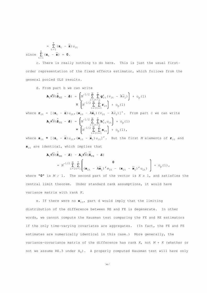
T -----= S (z - z)ut it
t=1T -----
since S (z - z) = 0.tt=1
c. There is really nothing to do here. This is just the usual first-
order representation of the fixed effects estimator, which follows from the
general pooled OLS results.
d. From part b we can write
N T----- ^ & -1/2 ----- *A rN(D - D) = N S S g’ (v - lv ) + o (1)1 RE it it i p7 8i=1t=1
N T& -1/2 *_ N S S r + o (1)it p7 8i=1t=1
----- ----- -----where r = [(z - z)u ,(x - lx )(v - lv )]’. From part c we can writeit t it it i it i
N T----- ^ & -1/2 *A rN(D - D) = N S S h’ u + o (1)2 FE it it p7 8i=1t=1
N T& -1/2 *_ N S S s + o (1),it p7 8i=1t=1
----- -----where s _ [(z - z)u ,(x - x )u ]’. But the first M elements of r andit t it it i it it
s are identical, which implies thatit
----- ^ ----- ^A rN(D - D) - A rN(D - D)1 RE 2 FE
& *N T 0-1/2= N S S 2 2 + o (1),----- ----- p
i=1t=1 (x - lx )’e - (x - x )’u )7 it i it it i it 8
where "0" is M * 1. The second part of the vector is K * 1, and satisfies the
central limit theorem. Under standard rank assumptions, it would have
variance matrix with rank K.
e. If there were no x , part d would imply that the limitingit
distribution of the difference between RE and FE is degenerate. In other
words, we cannot compute the Hausman test comparing the FE and RE estimators
if the only time-varying covariates are aggregates. (In fact, the FE and FE
estimates are numerically identical in this case.) More generally, the
variance-covariance matrix of the difference has rank K, not M + K (whether or
not we assume RE.3 under H ). A properly computed Hausman test will have only0
147

K degrees-of-freedom, not M + K, as is often resported by econometrics
packages. The regression-based test described in Problem 10.9 makes the
degeneracies obvious, and it is easily made robust in Stata using the "xtgee"
command.
148