solutions to selected problems in: reinforcement learning...
TRANSCRIPT
Solutions to Selected Problems In:
Reinforcement Learning: An Introduction
by Richard S. Sutton and Andrew G. Barto.
John L. Weatherwax∗
March 26, 2008
Chapter 1 (Introduction)
Exercise 1.1 (Self-Play):
If a reinforcement learning algorithm plays against itself it might develop a strategy wherethe algorithm facilitates winning by helping itself. In other words it might alternate between“good” moves and “bad” moves in such a way that the algorithm wins every game. Thus itwould seem that the algorithm would not learn a min/max playing strategy.
Exercise 1.2 (Symmetries):
We could improve our reinforcement learning algorithm by taking advantage of symmetryby simplifying the definition of the “state” and “action” upon which the algorithm wouldworks. By simplifying the state in such a way that the dimension decreases we can be moreconfident that our learned results will be statistically significant since the state space weoperate in is reduced. If our opponent was taking advantage of symmetries in the gametic-tac-toe our algorithm should also since this fact, would enable us to be a better gameplayer against this type of player. If our player does not use symmetries then our algorithmshould not either (except to reduce the state space as discussed above) since enforcing asymmetry on our opponent (that is not in fact there) should decrease our performance whenplaying against this type of opponent.
1
Exercise 1.3 (Greedy Play):
As will be discussed later in this book a greedy approach will not be able to learn moreoptimal moves as play unfolds. Thus there is a natural trade-off between attempting toexplore the space of possibilities and selecting the action on this step that has the greatestreward. Problems with direct greedy play would be that our player fails to be able tocapture moves that result in improved rewards because we never take a chance on unknown(or unexplored) actions.
Exercise 1.4 (Learning from Exploration):
If we do not learn from exploratory moves then the state probabilities learned would effec-tively be random in that we are not updating our undertaking of what happens when in agiven state and a given action is taken. If we learn from our exploratory moves then ourlimiting probabilities should be those from the desired distribution of state and action selec-tions. Obviously a more complete understanding of the probability densities should resultin a better play since the player better understands the “game” he or she is playing.
Exercise 1.5 (Other Improvements):
One possible way would be to have a saved library of scripted plays. For example the logicwould be something like, when in a set of known states always execute the following moves.This is somewhat like the game of chess where there are various “opening” positions thatexpert players have deemed good. Hopefully this might expedite the total learning processor at least improve our reinforcement players initial play.
Since the the tic-tac-toe problem is so simple we can solve this problem (using recursion) andcomputing all possible opponents moves and selecting at each step the move that optimizesour chance of winning. This is in fact a common introductory programming exercise.
Chapter 2 (Evaluative Feedback)
Action-Value Methods
See the Matlab file n armed testbed.m for code to generate the plots shown in Figure 2.1of the book. We performed experiments with two different values for the standard deviationof the rewards received: 1 and 10.
Exercise 2.1 (Discussions on the 10-armed testbed):
Plotting both the cumulative average reward and the cumulative percent optimal actionwe see that in both cases the strategy with more exploration i.e. ǫ = 0.1 will produce alarger cumulative reward and larger percentage of time the optimal reward is obtained. For1000 plays the ǫ = 0.1 strategy obtains a cumulative total reward of about 1300 while thegreedy strategy obtains a total reward of about 1000 or an improvement of 30%. The aboveexperiment is with the reward variance from each “arm” set at 1.0.
When we set the variance of each random draw to a larger number say σ2 = 10.0 we see thesame pattern.
I’ll mention a very simple approach that greatly improves the performance of the greedyalgorithm. This idea is motivated by the algorithms described in the book where they all startno knowledge of the true reward function Q∗(a). These algorithms initially approximatesthis at t = 0 with zero values before beginning of each strategy. If instead, we allow ouralgorithm to take one draw on each arm and uses the observed values that result as its initialapproximation for Q∗(a) the performance is considerably improved. If the variance of therewards on each arm is small then this set of initial trials will yield relatively good resultssince we have a very simple estimate (a single sample) of the rewards from each arm.
Softmax-Action-Selection
Exercise 2.2 (programming softmax-action selection):
See the Matlab file n armed testbed softmax.m for code to generate plots similar to thoseshown in Figure 2.1 of the book but using softmax action selection.
Exercise 2.3 (the logistic or sigmoid function):
With two actions (say x andy) the Gibbs distribution discussed in this section requirescomparing the following two probabilities
ex/τ
ex/τ + ey/τand
ey/τ
ex/τ + ey/τ.
By multiplying the first expression by e−x/τ on the top and the bottom we obtain
1
1 + e(y−x)/τ,
which is the definition of the logistic function. The temperature τ here plays the role of howquickly the incoming signal is “squashed”. The larger τ is the more quickly the functionsquashes its inputs and the distribution becomes uniform.
Evaluation versus Instruction
See the Matlab files binary bandit exps.m and binary bandit exps Script.m for code togenerate the plots shown in Figure 2.3 of the book. In addition, we plot the results fortwo “easy” problems denoted as the upper left and lower right corners of the diagram inFigure 2.2. These easy problems are where p1 = 0.05 and p2 = 0.85 and pA = 0.9 andpB = 0.1.
Incremental Implementation
Exercise 2.5 (the n-armed bandit with α = 1/k):
See the Matlab files exercise 2 5.m for code to simulate the n-armed bandit problem, withgreedy action selection and incremental computation of action values (here α = 1/k).
Tracking a Non-stationary Problem
Exercise 2.6:
We are told in this problem that the step sizes, αk(a), are not constant with the timestep buthave a k dependence. Following the discussion in the book we will derive an expression forQk in terms of its initial specification Q0, the received rewards rk, and the step size valuesαk. Now for each action a our action-value estimate is updated using
Qk = Qk−1 + αk(rk −Qk−1) ,
where we have dropped the dependence on the action taken (i.e. a) for notational simplicity.In the above formula we can recursively substitute for the earlier terms (e.g. replace Qk−1
with an expression involving Qk−2) to obtain the desired expression. We will follow thisprescription until the pattern is clear and at that point generalize. We find
Qk = Qk−1 + αk(rk −Qk−1)
= αkrk + (1− αk)Qk−1
= αkrk + (1− αk) [αk−1rk−1 + (1− αk−1)Qk−2]
= αkrk + (1− αk)αk−1rk−1 + (1− αk)(1− αk−1)Qk−2
= αkrk + (1− αk)αk−1rk−1 + (1− αk)(1− αk−1) [αk−2rk−2 + (1− αk−2)Qk−3]
= αkrk + (1− αk)αk−1rk−1 + (1− αk)(1− αk−1)αk−2rk−2
+ (1− αk)(1− αk−1)(1− αk−2)Qk−3
= · · ·= αkrk + (1− αk)αk−1rk−1 + (1− αk)(1− αk−1)αk−2rk−2 + · · ·

+ (1− αk)(1− αk−1)(1− αk−2) · · · (1− α3)α2r2
+ (1− αk)(1− αk−1)(1− αk−2) · · · (1− α2)α1r1
+ (1− αk)(1− αk−1)(1− αk−2) · · · (1− α2)(1− α1)Q0 .
Thus in the general case the weight on the prior reward Q0 is given by∏k
i=1(1− αi).
Exercise 2.7:
See the Matlab files exercise 2 7.m and exercise 2 7 Script.m for code to simulate then-armed bandit problem on a non-stationary problem. As suggested in the problem givenan initial set of action values Q∗(a) on each timestep the action values take a random walk.That is at the next timestep they are given by
Q∗(a) = Q∗(a) + σRWdW ,
where dW is a random variable drawn from a standard normal. We have introduced a variableσRW that determines how much non-stationary is introduced at each step. We expect that asσRW increases the sample-average method will perform increasingly worse than the action-value method with a constant step size α. This can be seen from the experiments performedwith the code.
Optimistic Initial Values
See the Matlab files opt initial values.m and opt initial values Script.m for code togenerate the plots shown in Figure 2.4 of the book.
Exercise 2.8:
If the initial play selected when using the optimistic method are by chance ones of the better
choices then the action value estimates Q(a) for these plays will be magnified resulting in anemphasis to continue playing this action. This results in large actions values being receivedon the initial draws and consequently very good initial play. In the same way, if the algorithminitially selects poor plays then initially the algorithm will perform poorly resulting in verypoor initial play.
Reinforcement Comparison
See the Matlab files reinforcement comparison methods.m and the driver “Script” file forcode to generate the plots shown in Figure 2.5 of the book.
Exercise 2.9:
The fact that the temperature parameter is not found in the softmax relationship for thisproblem is not a problem since we introduce another constant β in our action preferenceupdate equation. This parameter β has the affect of various temperature settings in a Gibbslike probability update.
Exercise 2.10:
The α parameter in the reference reward update equation determines how fast we convergeto a reference value α = 0 and convergence is immediate where when α = 1 the sequencer̄t changes with each reward. The same comments apply to the action preferences pt(a) andthe parameter β. Since at the beginning of our experiments we don’t know either of theseunknowns the reference reward value r̄ or the action preferences p(a) to appropriately learnthese we need two parameters. If we set α = β we would effectively be enforcing that therate of convergence of each of the estimates should be the same.
Exercise 2.11:
The action preference update equation is modified as follows
pt+1(at) = pt(at) + β(rt − r̄t)(1− πt(at)) .
This modification is implemented in the Matlab file exercise 2 11.m, and the driver “Script”file. The plots produced by this code indeed show that the addition of this factor does indeedimprove the performance of the algorithm.
Pursuit Methods
See the Matlab files persuit method.m and persuit method Script.m for code to generatethe plots shown in Figure 2.6 of the book.
Exercise 2.12:
The persuit algorithm is not guaranteed to always select the optimal action. For example ifthe initial rewards are such that we incorrectly update the wrong actions, causing π(a) tobecome biased away from its true value we could never actually draw from the optimal arm.Setting the initial action probabilities equal to a uniform distribution helps this. In the casewhere the prior distributions are set such that π = 1 for a specific arm and π = 0 for allothers emphasizes the fact that the algorithm does not fully explore the state space.
Exercise 2.15:
One idea is to have the algorithm perform an ǫ-persuit algorithm where ǫ percent of the timewe randomly try an arm. The remaining 1 − ǫ amount of the time we follow the standardpersuit algorithm. Thus even if the action probabilities πt(a) converge to something incorrectthe fact that ǫ percent of the time we are selecting a random arm means that in enough trialswe will explore the entire space.
As a practical detail, we could code our methods so that on the ǫ percent of the time it isexploring it is explicitly forbidden from drawing on the “greedy” arm. This would be thearm that would be most likely be selected using the action probabilities πt. That is, don’tdraw on the arm a∗ given by
a∗ = ArgMaxa(πt(a)) .
This modification may help in the exploration process since we don’t waste an exploratorydraw.
Associative Search
Exercise 2.16 (unknown bandits):
If you are not told which of the cases of the problem one faces, we can assume that onaverage half of the time we will be facing a case A instance and half of the time a case Binstance. In general if we knew which case we were facing we would like to pull differentarms (the optimal play would be to pull the second arm in the case of A instance and pullthe first arm in the case of a case B instance). Since we have no knowledge the best we canobtain is the average reward. The expectation of playing each type of game (assuming thatwe have no way to select which arm to pull and we select randomly ) is given by
E[A] = 0.5(0.1) + 0.5(0.9) = 0.5
E[B] = 0.5(0.2) + 0.5(0.8) = 0.5 .
So assuming a uniform distribution over which type of case we are given and where we playmany games is given by
0.5(0.5) + 0.5(0.5) = 0.5 .
In the case where one is told which case one is playing one could learn the optimal arm topull in each case and then play that arm repeatedly. In this case the expected reward forplaying many times is given by
0.5(0.2) + 0.5(0.9) = 0.55 ,
thus we see that when we know the type of the game we are playing our expected rewardincreases as one would expect.
Chapter 3 (The Reinforcement Learning Problem)
The Agent-Environment Interface
Exercise 3.1 (examples of reinforcement learning tasks):
One example might be the robot learning of how to escape a maze. The state could bethe robots position (and directional heading) in the maze. The actions could be one of thefollowing: to move forward, backwards, or sideways. The reward could be negative one ifthe robot collided with a wall and/or plus one once the solution to the maze is found.
Another example might be a reinforcement algorithm aimed a learning how to drive a cararound a race track. The state could be a vector representing the distance to each of thelateral sides (the walls to the left and right of the car), the directional heading, the velocityand acceleration of the car. The actions could be to change any of the state vectors i.e.to accelerate or decelerate or to change heading. The rewards could be zero if the car isproceeding comfortably along and minus one if the car collides with a wall.
A third example might be learning the optimal time to buy or sell securities given someinformation about the current state of the securities return. In this case the state would bethe magnitude and direction of the instantaneous return, the action might be the size of aposition to take (how much of a security to buy or sell) and whether to buy or sell. Thereward might be the corresponding profit or loss from this action. One would hope that overtime the reinforcement learning algorithm would learn how much and the given direction totake to maximize a profit.
Exercise 3.2 (other goal directed learning tasks):
One difficulty could be with learning tasks that result in a vector of rewards rather than justa scalar. In this case one is trying to maximize simultaneously several things. If there is noclear way to reduce this to a scalar problem it might be unclear how to apply reinforcementlearning ideas. One way to produce a scalar problem is to come up with a set of “weights”and take the inner product of the rewards with these weights.
Exercise 3.3 (driving as a reinforcement task):
The correct level at which to define the agent and the environment depends on what taskone wants to use the algorithm for. For example if one wants to model the car interactingwith the road it maybe simpler to use the situation where we model the implied torqueson the wheels. If one however want to model interacting drivers on various roads then itmaybe better to model everything at a much higher level, where we are considering “where”

to drive. For any given task some information maybe easier to obtain and may guide themodeler in selecting the level to work at.
Returns
Exercise 3.4 (pole-balancing as an episodic task):
In this case the returns at each time will be related to −γk as before but only up to some Kless than the episode end time T . This differs in that they is a ceiling (−γT ) above whichthe returns cannot get larger than.
Exercise 3.5 (running in a maze):
You have not communicated a “time limit” to the robot in this formulation. Since the agentsuffers no loss while exploring the maze one possible solution is to explore until our episodeof time elapses. Since we want our robot to actively seek out a solution to the maze problembetter performance may result if we prescribe a reward of −1 (or a penalty) for each timestepthe robot spends in the maze without finding the exit.
The Markov Property
Exercise 3.6 (broken vision system):
In a general principles, to have a Markov state means that the knowledge of this stateis sufficient to predict the next state and the expected reward given some action. Sincewe cannot see everything the photograph of the objects does not contain the entirety ofinformation needed to next predict what state (image) we will be presented with next. Forexample, we don’t know if something will pass over our head from behind us and land inour field of view. If we assume that everything we will ever see is in front of us then notknowing the objects velocities prevents us from having a full Markov state. If we assume thateverything is stationary then we would might say that we had a Markov state. Obviously ifour camera was broken for some length of time we would not be able to predict fully in thefuture what we might see and the last known image would not be a Markov state.
Markov Decision Processes
Exercise 3.7 (linking transition probabilities and expected rewards):
Consider first the expression for the expected next reward Ras,s′. This is defined as the
expectation of the reward rt+1 given the current state, the action taken, and the next statei.e.
Ras,s′ = E{rt+1|st = s, at = a, st+1 = s′} .
By the definition of expectation this is equal to
∑
r′r′P{rt+1 = r′|st = s, at = a, st+1 = s′} .
Where the sum is over all of the finite possible rewards r′. By the definition of conditionalprobability, the probability in the above can be written in terms of the joint conditionaldistribution as
P{rt+1 = r′|st = s, at = a, st+1 = s′} =P{st+1 = s′, rt+1 = r′|st = s, at = a}
P{st+1 = s′|st = s, at = a} .
In the above we recognize the denominator as equal to the definition of our transition prob-abilities for our finite Markov decision process namely P a
s,s′. Thus we obtain
Ras,s′ =
∑
r′r′
P{st+1 = s′, rt+1 = r′|st = s, at = a}P a
s,s′.
Multiplying both sides by P as,s′ we finally obtain the desired relationship
Ras,s′P
as,s′ =
∑
r′r′P{st+1 = s′, rt+1 = r′|st = s, at = a} .
Value Functions
I found it necessary to consider the derivation of Bellman’s equation in more detail, whichI do here. Remembering that the definition of V π(s) is given by Eπ{Rt|st = s}, and Rt =∑∞
k=0 γkrt+k+1 we have the first set of equations given in the book. That is
V π(s) = Eπ{Rt|st = s}
= Eπ{∞∑
k=0
γkrt+k+1|st = s}
To evaluate this expectation we will use the conditional expectation theorem which statesthat one can evaluate the expectation of a random variable say X by conditioning on allpossible other events (here Y and Y c). Mathematically, this statement is
E[X] = E[X|Y ]P{Y }+ E[X|Y c]P{Y c} .
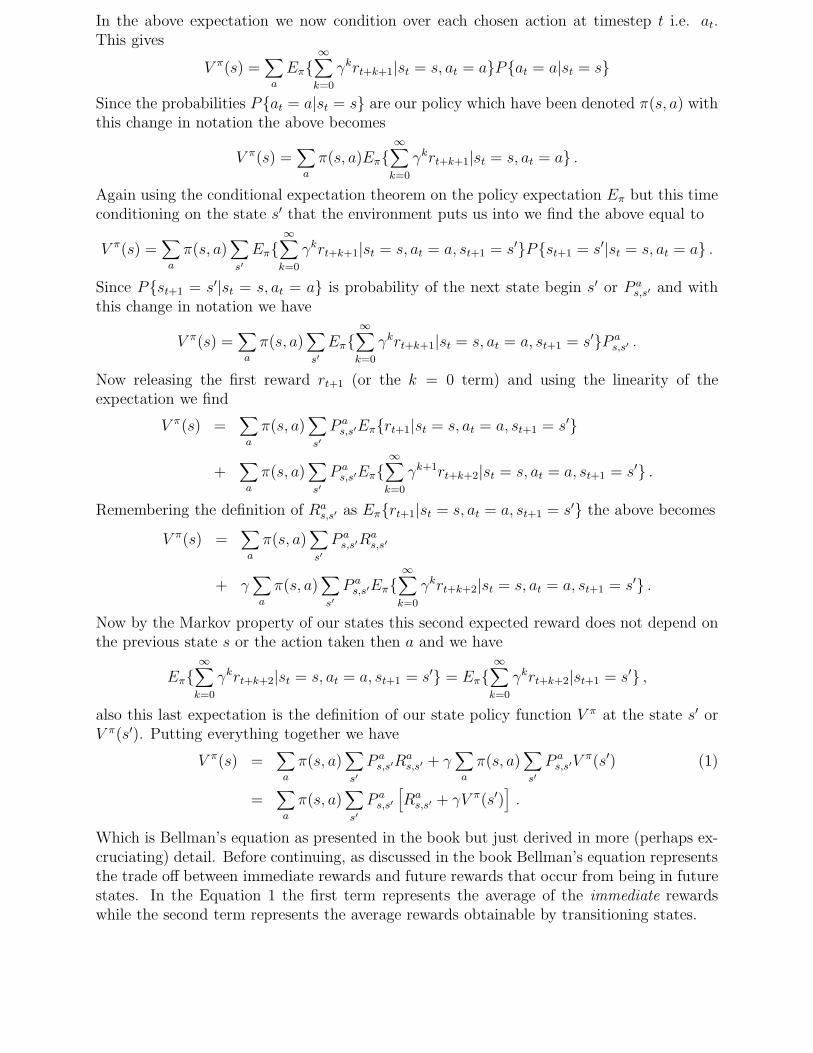
In the above expectation we now condition over each chosen action at timestep t i.e. at.This gives
V π(s) =∑
a
Eπ{∞∑
k=0
γkrt+k+1|st = s, at = a}P{at = a|st = s}
Since the probabilities P{at = a|st = s} are our policy which have been denoted π(s, a) withthis change in notation the above becomes
V π(s) =∑
a
π(s, a)Eπ{∞∑
k=0
γkrt+k+1|st = s, at = a} .
Again using the conditional expectation theorem on the policy expectation Eπ but this timeconditioning on the state s′ that the environment puts us into we find the above equal to
V π(s) =∑
a
π(s, a)∑
s′Eπ{
∞∑
k=0
γkrt+k+1|st = s, at = a, st+1 = s′}P{st+1 = s′|st = s, at = a} .
Since P{st+1 = s′|st = s, at = a} is probability of the next state begin s′ or P as,s′ and with
this change in notation we have
V π(s) =∑
a
π(s, a)∑
s′Eπ{
∞∑
k=0
γkrt+k+1|st = s, at = a, st+1 = s′}P as,s′ .
Now releasing the first reward rt+1 (or the k = 0 term) and using the linearity of theexpectation we find
V π(s) =∑
a
π(s, a)∑
s′P a
s,s′Eπ{rt+1|st = s, at = a, st+1 = s′}
+∑
a
π(s, a)∑
s′
P as,s′Eπ{
∞∑
k=0
γk+1rt+k+2|st = s, at = a, st+1 = s′} .
Remembering the definition of Ras,s′ as Eπ{rt+1|st = s, at = a, st+1 = s′} the above becomes
V π(s) =∑
a
π(s, a)∑
s′P a
s,s′Ras,s′
+ γ∑
a
π(s, a)∑
s′P a
s,s′Eπ{∞∑
k=0
γkrt+k+2|st = s, at = a, st+1 = s′} .
Now by the Markov property of our states this second expected reward does not depend onthe previous state s or the action taken then a and we have
Eπ{∞∑
k=0
γkrt+k+2|st = s, at = a, st+1 = s′} = Eπ{∞∑
k=0
γkrt+k+2|st+1 = s′} ,
also this last expectation is the definition of our state policy function V π at the state s′ orV π(s′). Putting everything together we have
V π(s) =∑
a
π(s, a)∑
s′P a
s,s′Ras,s′ + γ
∑
a
π(s, a)∑
s′P a
s,s′Vπ(s′) (1)
=∑
a
π(s, a)∑
s′P a
s,s′
[
Ras,s′ + γV π(s′)
]
.
Which is Bellman’s equation as presented in the book but just derived in more (perhaps ex-cruciating) detail. Before continuing, as discussed in the book Bellman’s equation representsthe trade off between immediate rewards and future rewards that occur from being in futurestates. In the Equation 1 the first term represents the average of the immediate rewardswhile the second term represents the average rewards obtainable by transitioning states.
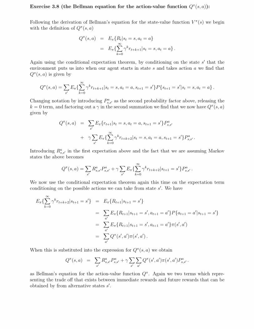
Exercise 3.8 (the Bellman equation for the action-value function Qπ(s, a)):
Following the derivation of Bellman’s equation for the state-value function V π(s) we beginwith the definition of Qπ(s, a)
Qπ(s, a) = Eπ{Rt|st = s, at = a}
= Eπ{∞∑
k=0
γkrt+k+1|st = s, at = a} .
Again using the conditional expectation theorem, by conditioning on the state s′ that theenvironment puts us into when our agent starts in state s and takes action a we find thatQπ(s, a) is given by
Qπ(s, a) =∑
s′Eπ{
∞∑
k=0
γkrt+k+1|st = s, at = a, st+1 = s′}P{st+1 = s′|st = s, at = a} .
Changing notation by introducing P as,s′ as the second probability factor above, releasing the
k = 0 term, and factoring out a γ in the second summation we find that we now have Qπ(s, a)given by
Qπ(s, a) =∑
s′Eπ{rt+1|st = s, at = a, st+1 = s′}P a
s,s′
+ γ∑
s′Eπ{
∞∑
k=0
γkrt+k+2|st = s, at = a, st+1 = s′}P as,s′ .
Introducing Ras,s′ in the first expectation above and the fact that we are assuming Markov
states the above becomes
Qπ(s, a) =∑
s′Ra
s,s′Pas,s′ + γ
∑
s′Eπ{
∞∑
k=0
γkrt+k+2|st+1 = s′}P as,s′ .
We now use the conditional expectation theorem again this time on the expectation termconditioning on the possible actions we can take from state s′. We have
Eπ{∞∑
k=0
γkrt+k+2|st+1 = s′} = Eπ{Rt+1|st+1 = s′}
=∑
a′
Eπ{Rt+1|st+1 = s′, at+1 = a′}P{at+1 = a′|st+1 = s′}
=∑
a′
Eπ{Rt+1|st+1 = s′, at+1 = a′}π(s′, a′)
=∑
a′
Qπ(s′, a′)π(s′, a′) .
When this is substituted into the expression for Qπ(s, a) we obtain
Qπ(s, a) =∑
s′
Ras,s′P
as,s′ + γ
∑
s′
∑
a′
Qπ(s′, a′)π(s′, a′)P as,s′ .
as Bellman’s equation for the action-value function Qπ. Again we two terms which repre-senting the trade off that exists between immediate rewards and future rewards that can beobtained by from alternative states s′.
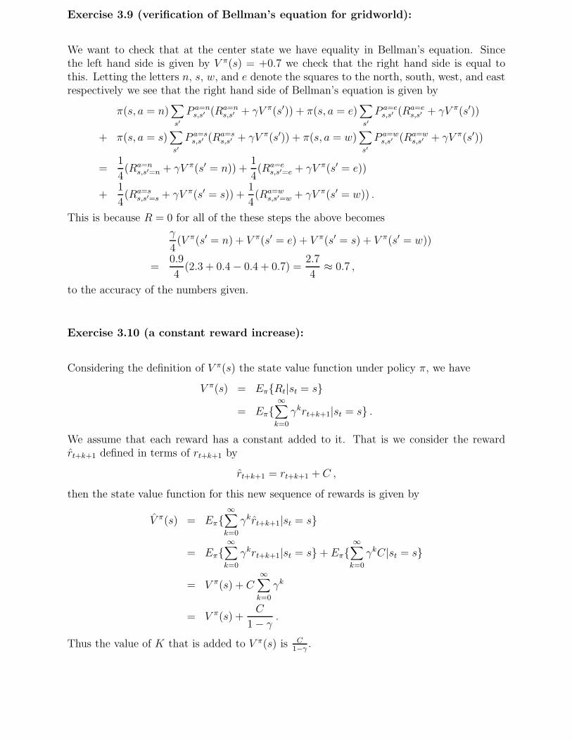
Exercise 3.9 (verification of Bellman’s equation for gridworld):
We want to check that at the center state we have equality in Bellman’s equation. Sincethe left hand side is given by V π(s) = +0.7 we check that the right hand side is equal tothis. Letting the letters n, s, w, and e denote the squares to the north, south, west, and eastrespectively we see that the right hand side of Bellman’s equation is given by
π(s, a = n)∑
s′P a=n
s,s′ (Ra=ns,s′ + γV π(s′)) + π(s, a = e)
∑
s′P a=e
s,s′ (Ra=es,s′ + γV π(s′))
+ π(s, a = s)∑
s′P a=s
s,s′ (Ra=ss,s′ + γV π(s′)) + π(s, a = w)
∑
s′P a=w
s,s′ (Ra=ws,s′ + γV π(s′))
=1
4(Ra=n
s,s′=n + γV π(s′ = n)) +1
4(Ra=e
s,s′=e + γV π(s′ = e))
+1
4(Ra=s
s,s′=s + γV π(s′ = s)) +1
4(Ra=w
s,s′=w + γV π(s′ = w)) .
This is because R = 0 for all of the these steps the above becomes
γ
4(V π(s′ = n) + V π(s′ = e) + V π(s′ = s) + V π(s′ = w))
=0.9
4(2.3 + 0.4− 0.4 + 0.7) =
2.7
4≈ 0.7 ,
to the accuracy of the numbers given.
Exercise 3.10 (a constant reward increase):
Considering the definition of V π(s) the state value function under policy π, we have
V π(s) = Eπ{Rt|st = s}
= Eπ{∞∑
k=0
γkrt+k+1|st = s} .
We assume that each reward has a constant added to it. That is we consider the rewardr̂t+k+1 defined in terms of rt+k+1 by
r̂t+k+1 = rt+k+1 + C ,
then the state value function for this new sequence of rewards is given by
V̂ π(s) = Eπ{∞∑
k=0
γkr̂t+k+1|st = s}
= Eπ{∞∑
k=0
γkrt+k+1|st = s}+ Eπ{∞∑
k=0
γkC|st = s}
= V π(s) + C∞∑
k=0
γk
= V π(s) +C
1− γ.
Thus the value of K that is added to V π(s) is C1−γ
.
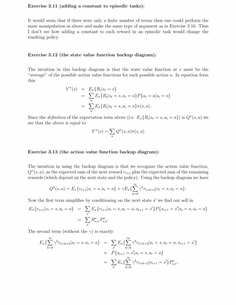
Exercise 3.11 (adding a constant to episodic tasks):
It would seem that if there were only a finite number of terms then one could perform thesame manipulation as above and make the same type of argument as in Exercise 3.10. ThusI don’t see how adding a constant to each reward in an episodic task would change theresulting policy.
Exercise 3.12 (the state value function backup diagram):
The intuition in this backup diagram is that the state value function at s must be the“average” of the possible action value functions for each possible action a. In equation formthis
V π(s) = Eπ{Rt|st = s}=
∑
a
Eπ{Rt|st = s, at = a}P{at = a|st = s}
=∑
a
Eπ{Rt|st = s, at = a}π(s, a) .
Since the definition of the expectation term above (i.e. Eπ{Rt|st = s, at = a}) is Qπ(s, a) wesee that the above is equal to
V π(s) =∑
a
Qπ(s, a)π(s, a)
Exercise 3.13 (the action value function backup diagram):
The intuition in using the backup diagram is that we recognize the action value function,Qπ(s, a), as the expected sum of the next reward rt+1 plus the expected sum of the remainingrewards (which depend on the next state and the policy). Using the backup diagram we have
Qπ(s, a) = Eπ{rt+1|st = s, at = a} + γEπ{∞∑
k=0
γkrt+k+2|st = s, at = a} .
Now the first term simplifies by conditioning on the next state s′ we find our self in
Eπ{rt+1|st = s, at = a} =∑
s′Eπ{rt+1|st = s, at = a, st+1 = s′}P{st+1 = s′|st = s, at = a}
=∑
s′Ra
s,s′Pas,s′
The second term (without the γ) is exactly
Eπ{∞∑
k=0
γkrt+k+2|st = s, at = a} =∑
s′Eπ{
∞∑
k=0
γkrt+k+2|st = s, at = a, st+1 = s′}
× P{st+1 = s′|st = s, at = a}
=∑
s′Eπ{
∞∑
k=0
γkrt+k+2|st+1 = s′}P as,s′ ,
since the sum of rewards (∑∞
k=0 γkrt+k+2) are received at times t + 1 onward at which point,after conditioning we are in state s′ and the previous state s and action a give no information(assuming our states are Markov). Finally, replacing the expectation
Eπ{∞∑
k=0
γkrt+k+2|st+1 = s′}
with V π(s′) we have shown that Qπ(s, a) is equal to
Qπ(s, a) =∑
s′
(Ras,s′ + γV π(s′))P a
s,s′ ,
Optimal Value Functions
See the Matlab code rr state bellman.m for code to numerically evaluate the optimalBellman equations for the recycling robot.
Exercise 3.14 (the optimal state-value function for golf):
If we assume a penalty (reward) of −1 for each stroke we take to get the ball in the hole, theoptimal state-value function V ∗(s) gives the expected number of swings to get the ball inthe hole using any type of club. Thus where we expect it to take many swings to get the ballin the hole using just a putter, we expect that using both a putter and a driver would allowone to get the ball in the hole in a quicker amount of time. Thus the optimal state-valuefunction for golf would qualitatively like that given in Figure 3.6 but would have smallernumbers on the outlying contours. This is because using both types of clubs we expect tobe able to get the ball in the hole in fewer swings than just using the putter.
Exercise 3.15 (the contours of the optimal action-value for putting):
The optimal action-value function Q∗(s, putter) means that we take the action of using aputter and then follow the optimal policy from that point onward. I would expect thattaking a putter first would be the optimal action for region of state space that are close tothe hole and this state value function would give an expected number of swings that werequite small. For regions of state space further away from the hole I would expect the choiceof using a putter as the first club to not be optimal and this would give action-value statesthat are slightly lower (and requiring more swings) in these regions of state space.
Exercise 3.16 (the Bellman equation for the recycling robot):
Bellman’s optimal equation for Q∗(s, a) is given by
Q∗(s, a) =∑
s′P a
s,s′(Ras,s′ + γ max
a′
Q(s′, a′)) .
We will evaluate this function for all the possible states the robot can be in and all thecorresponding actions the robot can take when in those states. To begin, if the robots is inthe state of “high” (h) (with any action a) the above becomes
Q∗(h, a) =∑
s′P a
h,s′(Rah,s′ + γ max
a′
Q∗(s′, a′)) .
In the high state the allowable actions are to either search (s) or wait (w). If we search, thepossible next states the environment would put us in are either high or low (l). Evaluatingthe above assuming an action of searching and summing over all possible resulting statesgives the following
Q∗(h, s) =∑
s′∈{h,l}
P sh,s′(R
sh,s′ + γ max
a′
Q∗(s′, a′))
= P sh,h(R
sh,h + γ max
a′
Q∗(h, a′)) + P sh,l(R
sh,l + γ max
a′
Q∗(l, a′)) .
Using the definition of the various transition probabilities and one step rewards we defineP s
h,h = α, P sh,l = 1− α, Rs
h,h = Rs, and Rsh,l = Rs so that the above becomes
Q∗(h, s) = α(Rs + γ maxa′
Q∗(h, a′)) + (1− α)(Rs + γ maxa′
Q∗(l, a′))
= Rs + αγ max{Q∗(h, s), Q∗(h, w)}+ (1− α)γ max{Q∗(l, s), Q∗(l, w), Q∗(l, rc)} .
In the same way, we can evaluate the action-value function Q∗(h, w) which is the situationwhere we begin in a high state and perform the action of waiting (w). In this case we find
Q∗(h, w) = P wh,h(R
wh,h + γ max
a′
(Q∗(h, a′)) + P wh,l(R
wh,l + γ max
a′
Q∗(l, a′))
= Rw + γ max{Q∗(h, s), Q∗(h, w)} .
Since P wh,h = 1 and P w
h,l = 0. Continuing the process we have action-value function when weare in a low state and we search, wait, or recharge (rc) given by as the following. For Q∗(l, s)we have the following
Q∗(l, s) = P sl,h(R
sh,l + γ max
a′
(Q∗(h, a′)) + P sl,l(R
sl,l + γ max
a′
Q∗(l, a′))
= (1− β)(−3 + γ max{Q∗(h, s), Q∗(h, w)})+ β(Rs + γ max{Q∗(l, s), Q∗(l, w), Q∗(l, rc)} .
For Q∗(l, w) the following
Q∗(l, w) = P wl,h(R
wl,h + γ max
a′
Q∗(h, a′)) + P wl,l(R
wl,l + γ max
a′
Q∗(l, a′))
= Rw + γ max{Q∗(l, s), Q∗(l, w), Q∗(l, rc)} .
Since P wl,h = 0 and P w
l,l = 1. Finally, we find that Q∗(l, rc) given by
Q∗(l, rc) = P rcl,h(R
rcl,h + γ max
a′
Q∗(h, a′)) + P rcl,l (R
rcl,l + γ max
a′
Q∗(l, a′))
= γ max{Q∗(h, s), Q∗(h, w)} .
Here for future reference we will list the optimal entire Bellman’s system for the recyclingrobot example. We have that
Q∗(h, s) = Rs + αγ max{Q∗(h, s), Q∗(h, w)}+ (1− α)γ max{Q∗(l, s), Q∗(l, w), Q∗(l, rc)}
Q∗(h, w) = Rw + γ max{Q∗(h, s), Q∗(h, w)}Q∗(l, s) = (1− β)(−3 + γ max{Q∗(h, s), Q∗(h, w)})
+ β(Rs + γ max{Q∗(l, s), Q∗(l, w), Q∗(l, rc)}Q∗(l, w) = Rw + γ max{Q∗(l, s), Q∗(l, w), Q∗(l, rc)}Q∗(l, rc) = γ max{Q∗(h, s), Q∗(h, w)} .
These could be solved by iteration once appropriate constants are specified. See the filerr action bellman.m for Matlab code to numerically evaluate the optimal Bellman equa-tions for the recycling robot.
Exercise 3.17 (evaluation of the gridworld optimal state-value function):
By definition, V ∗(s) is given by
V ∗(s) = maxa∈A(s)
Eπ∗{Rt|st = s, at = a}
= maxa∈A(s)
Eπ∗{∞∑
k=0
γkrt+k+1|st = s, at = a} .
We begin by assuming that the optimal policy for this gridworld example is given in Fig-ure 3.8c. In addition, the rewards structure for this problem is known. Specifically, it isminus one if we step off the gridworld, +10 at the position (1, 2) (in matrix notation), a +5at the position (1, 4) and zero otherwise. Using this information we can explicitly computethe right hand side of the above expression for V ∗(s). We have that V ∗ at the state (1, 2) isgiven by
V ∗((1, 2)) = +10 + γ · 0 + γ2 · 0 + γ3 · 0 + γ4 · 0 + γ5 · 10 + · · ·In the above formula, the pattern of terms above will continue indefinitely. We now describehow each term comes about so that the pattern is clear. The term +10 is the constant rewardgiven by the environment when we are moved from the position (1, 2) to the position (5, 2).The term γ · 0 comes from the reward given when the optimal step from position (5, 2) to(4, 2) is taken. The term γ2 · 0 comes from the optimal step from the position (4, 2) to (3, 2)with a zero reward. The term γ3 · 0 comes from the optimal step from the position (3, 2) to(2, 2) with a zero reward. The term γ4 · 0 comes from the optimal step from the position(2, 2) to (1, 2) with a zero reward. This final step places us at the position (1, 2) and lets usreceive the next reward of +10 and gives the term +10γ5.
We can in fact explicitly evaluate the above sum. We find
V ∗((1, 2)) = 10 + 10γ5 + 10γ10 + · · ·
= 10∞∑
k=0
γ5k =10
1− γ5.
if γ = 0.9 the above sum to three decimal places is given by 24.419.
Chapter 4 (Dynamic Programming)
Policy Evaluation
See the Matlab code iter poly gw inplace.m (for inplace) and iter poly gw not inplace.m
(for otherwise) to duplicate the example from this section on policy evaluation for the grid-world example.
Exercise 4.1 (evaluate Qπ for some states and actions):
Using the result derived by considering the backup diagram between the action-value andstate-value functions in Exercise 3.13 we recall that our action-value function Q can bewritten in terms of our state-value function V as
Qπ(s, a) =∑
s′Ra
s,s′Pas,s′ + γ
∑
s′P a
s,s′Vπ(s′) .
For first case of interest (denoting the terminal state by T ) we have
Qπ(11, down) = Rdown11,T · 1 + γ · 1 · V π(T ) = 0 .
Since we are assuming that all of our actions are deterministic, the reward for transitioningto the terminal state is zero, and that the state-value function evaluated at the terminalstate is zero.
For the second case of interest we have
Qπ(7, down) = Rdown7,11 · 1 + γ · 1 · V π(11)
= −1− 14γ = −13.6 .
Here have assumed that movement to any non terminal state gives a reward of −1, γ = 0.9,and V π(11) = 14 (which is the value found from the policy iterations given in Figure 4.2).
Exercise 4.2 (the addition of a new state):
I’ll assume that the transitions from the original states being unchanged means that the state-value function values do not change for the original grid locations when this newly addedstate is appended. Then we can iterate Equation 4.5 to obtain the state value function atthis new state i.e. V π(15). We find that
V π(15) =∑
a
π(15, a)∑
s′P a
15,s′(Ra15,s′ + γV (s′))
=1
4(Rleft
15,12 + γV (12) + Rup15,13 + γV (13)
+ Rright15,14 + γV (14) + Rdown
15,15 + γV (15)) .
Putting in what we know for the values of V π(·) as given by the numbers in Figure 4.2 fromthe book we see that V π(15) should equal
V π(15) =1
4(−1− 22γ − 1− 20γ − 1− γ14− 1 + γV (15))
= −1− 14γ +γ
4V (15) .
When we solve the above for V (15) we get V (15) = −4(1+14γ)4−γ
. If we take γ = 0.9 then we
find V (15) = −17.548.
If the action from state 13 now takes the agent to state 15 the above analysis can be performfor both the values V π(15) and now V π(13). This would give two equations derived like theabove containing and these two unknowns. These two equations would then be solved forthe two values of V . We now discuss this implementation. The “steady state” equation thatV π must satisfy is given by
V π(s) =∑
a
π(s, a)∑
s′P a
s,s′(Ras,s′ + γV π(s′)) .
With a uniform probability policy π(s, a) = 14
we have that the above is given by
V π(s) =1
4
∑
a
∑
s′P a
s,s′(Ras,s′ + γV π(s′)) ,
and since the steps are deterministic
P as,s′ =
{
1 ifs′ = a0 ifs′ 6= a
,
i.e. we end up at the state our action desires, our state value function V π is given by
V π(s) =1
4(Rup
s,up + γV π(up) + Rdowns,down + γV π(down)
+ Rrights,right + γV π(right) + Rleft
s,left + γV π(left)) .
In the above, the notation Rups,up means that in state s we choose the action “up” which
deterministically transfers us to the state one square above that of s. Next, since the rewards
are negative one (unless we enter a terminal state which cannot happen for the states 13 or15 we are considering) the equation that V π(13) must satisfy is given by
V π(13) =1
4(−4 + γV π(9) + γV π(15) + γV π(14) + γV π(12))
= −1 +γ
4(−20 + V π(15)− 14− 22)
= −1 +γ
4(−56 + V π(15)) .
Also V π(15) satisfies the earlier equation
V π(15) =1
4(−4 + γV π(13) + γV π(15) + γV π(14) + γV π(12))
= −1 +γ
4(V π(13) + V π(15)− 14− 22)
= −1 +γ
4(V π(13) + V π(15))− 9γ .
Thus the system of equations to be solved for V π(13) and V π(15) is
V π(13)− γ
4V π(15) = −1− 14γ
−γ
4V π(13) +
(
1− γ
4
)
V π(15) = −1− 9γ .
Since this is a linear system for V π(13) and V π(15) we can solve it in a number of ways.When we take γ = 0.9 solving the above system gives
V π(13) = −17.3 and V π(15) = −16.7 .
Out of pure laziness this is solved in the Matlab file ex 4 2 sys solv.m.
Exercise 4.3 (sequential action-value function approximations):
From the Bellman’s equation for the action value function Qπ(s, a) derived in Exercise 3.8we have
Qπ(s, a) =∑
s′Ra
s,s′Pas,s′ + γ
∑
s′
∑
a′
Qπ(s′, a′)π(s′, a′)P as,s′ .
Now an algorithm for computing Qπ(s, a) can be obtained by using the rule of thumb: “turnequality into assignment”. To do this we can let Qk be the previous estimate of our actionvalue function Q under policy π insert it into the right hand side of the above to obtain anew approximation of Qπ on the left hand side. As an iteration equation this is
Qπk+1(s, a) =
∑
s′Ra
s,s′Pas,s′ + γ
∑
s′
∑
a′
Qπk(s′, a′)π(s′, a′)P a
s,s′ .
Exercise 4.4 (avoiding infinite iterations with unbounded value functions):
If the value function becomes unbounded for particular states as a practical matter wecan implement policy evaluation in such a way that we skip updating states whose valuefunction is more negative than some specified threshold. When this is done our policyevaluation algorithm will simply ignore these states and process the more important ones.If it happens that after policy evaluation all values of V are truncated by this threshold thisis an indication that our threshold was too small and should be increased.
Policy Iteration
See the Matlab codes jcr example.m, jcr policy evaluation.m, jcr policy improvement.m,and jcr rhs state value bellman.m for results that duplicate Figure 4.4 from the book.
Exercise 4.5 (jacks car rental programming):
Please see the Matlab files: ex 4 5 policy evaluation.m, ex 4 5 policy improvement.m,ex 4 5 rhs state value bellman.m, and ex 4 5 Script.m. The script ex 4 5 Script.m isthe main driver and produces plots similar (but modified for the specifics of this problem)to those shown in the book for the default jack’s car rental problem.
Exercise 4.6 (policy iteration for action value functions Q):
The algorithms for action value functions are the same in principle as those for state valuefunctions except that the action value function algorithms are considering a combined stateaction variable (s, a) rather than just a state variable s alone. With this observation, policyiteration for the action-value function Q then becomes
1. Initialize Q(s, a) and π(s) arbitrarily for every s ∈ S and a ∈ A(s).
2. Policy Evaluation
• Repeat
– ∆← 0
– For every (s, a) pair perform
∗ q ← Q(s, a)
∗ Update Q(s, a) using
Q(s, a)←∑
s′Ra
s,s′Pas,s′ + γ
∑
s′
∑
a′
Qπ(s′, a′)π(s′, a′)P as,s′ .
∗ ∆← max(∆, |q −Q(s, a)|)• Until ∆ < Θ (small positive number)
3. Policy Improvement:
• policy stable← True
• For every (s, a) pair perform
– p← π(s, a)
– π(s, a)← ArgMaxs,a(Qπ(s, a))
– if p 6= π(s, a) then policy stable← False
• if policy stable then stop; else go to Policy Evaluation step.
Here Θ is a numerical convergence parameter that determines how accurate our ultimatesolution is. To see that by using the algorithm we will continue to obtain better policiesrecall that V π must equal
V π =∑
a
Qπ(s, a)π(s, a) .
By picking our policy π(s, a) to be the one that is largest with respect to Q we will result ina policy π′ such that V π′
(s) ≥ V π(s) i.e. we have found a better policy. This final updateequation of π(s, a0 is also Equation 5.1 from the book.
Value Iteration
Exercise 4.8 (discussion of the gamblers problem):
The gamblers problem is particularly unstable, but for the configuration specified in thebook the policy seems to try to get to 100 in the fewest number of total flips.
Exercise 4.9 (programming the gamblers problem):
Please see the Matlab files: gam rhs state value bellman.m, and gam Script.m. Thescript gam Script.m is the main driver and produces plots similar (but modified for thespecifics of this problem).

Chapter 5 (Monte Carlo Methods)
Monte Carlo Policy Evaluation
See the Matlab code cmpt bj value fn.m, determineReward.m, shufflecards.m, handValue.mand stateFromHand.m for a set of functions that duplicates the results presented in Fig-ure 5.2.
Exercise 5.1 (observations about the value function for blackjack):
The value function jumps for the last two rows because these rows correspond to a playerwith a hand that sums to 20 or 21. These hand values are great enough that with a largeprobability the player will win the game and receive a reward of one. The drop of on the lastrow on the left is due to the fact that the dealer is showing an ace and that because of thishas a finite probability of getting blackjack or a large hand value and consequently winningthe game which would yield a result of negative one. The front most values in the casewhere the player has a usable ace are greater than when the player does not have a usableace because in the former case the player knows that one ace is held by himself leaving onlythree aces left and correspondingly lowering the probability that the dealer has one.
Monte Carlo Control
See the Matlab file mc es bj Script.m for code that uses Monte Carlo exploring starts tosolve the blackjack problem and to reproduce the plots in Figure 5.5 from the book.
On-Policy Monte Carlo Control
See the Matlab file soft policy bj Script.m for the computation of the optimal policy forblackjack using soft policy evaluation.
Off-Policy Monte Carlo Control
Exercise 5.4 (programming the racetrack example):
See the Matlab files ex 5 4 Script.m, mk rt.m, gen rt episode.m, init unif policy.m,mcEstQ.m, rt pol mod.m and velState2PosActions.m for code to solve the racetrack ex-ample using on-policy Monte Carlo control method.

Exercise 5.6 (a recursive formulation of a weighted average):
Given Eq 5.4 in the book i.e.
Vn =
∑nk=1 wkRk∑n
k=1 wk,
We can derive recursive formulas for Vn in the following way. We begin by incrementing nby one to get Vn+1 and releasing the last term wn+1 as
Vn+1 =
∑n+1k=1 wkRk∑n+1
k=1 wk
=
∑nk=1 wkRk + wn+1Rn+1
∑n+1k=1 wk
=
∑nk=1 wk
∑n+1k=1 wk
(
∑nk=1 wkRk∑n
k=1 wk
)
+
(
wn+1∑n+1
k=1 wk
)
Rn+1 .
Defining the sum of the weights as Wn =∑n
k=1 wk we see that the above is equal to
Vn+1 =Wn
Wn+1Vn +
wn+1
Wn+1Rn+1 .
Writing the first expression Wn
Wn+1as Wn+1−wn+1
Wn+1= 1− wn+1
Wn+1the above becomes
Vn+1 = Vn −wn+1
Wn+1
Vn +wn+1
Wn+1
Rn+1
= Vn −wn+1
Wn+1(Rn+1 − Vn) ,
as expected.
Exercise 5.7 (recursive formulation of the off-policy control algorithm):
To modify the off-policy control algorithm Figure 5.7 to use incremental weight computationwe need to modify the lines that compute N(s, a), D(s, a), and Q(s, a) with the directalgorithm. In the non-incremental algorithm these are given by direct update equations
N(s, a) ← N(s, a) + wRt
D(s, a) ← D(s, a) + w
Q(s, a) ← N(s, a)
D(s, a).
While in the incremental weight algorithm these quantities are computed (with D(s, a)initialized to zero) as
D(s, a) ← D(s, a) + w
Q(s, a) ← Q(s, a) +w
D(s, a)(Rt −Q(s, a)) .
Chapter 6 (Temporal Difference Learning)
Advantages of TD Prediction Methods
See the files mk fig 6 6.m and mk arms error plt.m for Matlab code to duplicate the twofigures from this section.
Exercise 6.1 (TD learning v.s. MC learning):
I would expect that TD learning would be much better than MC learning in the case wherewe are moved to a new building since this is just a change in our initial route and some ofthe state encountered during the general episode will be the same. For example, on our drivehome many of the states are the same once we enter the highway and the value functionestimates for these states obtained when we worked in the original building should be veryclose to what we will compute starting from our new building. Staring with a very goodinitial guess should result in faster convergence.
I would expect this same phenomena to happen in our original learning task if our initialguess at the value function is very close to that of the true value function.
Exercise 6.2 (discussions on TD learning on a random walk):
Since this problem in undiscounted, we have λ = 1, and taking α = 0.1 for the TD(0) updateexpression we obtain the following
V (st)← V (st) + 0.1(rt+1 + V (st+1)− V (st)) .
For transitions among states that do not end in one of the terminal states we receive a zeroreward, and since initially our value function begins as a constant our first update is givenby V (st)← V (st) or no change in the value function. If we terminate on the left our rewardis (taking V (st+1) = 0 when st+1 is the left most terminal state) that the state A is updatedas
V (A)← V (A) + 0.1(0 + 0− V (A)) = 0.9V (A) = 0.45 .
Which agrees with the plotted value of V (A) for the first iteration. Thus on the first episodethe random walk took us off the left end of the domain and we decreased our state valuefunction by 0.05.
Exercise 6.4 (grown of the RMS error):
Large values of α imply that more of V (s) is updated at each timestep. This in turn makes theTD(0) algorithm solution depend more heavily on the specific returns received at each step

of the specific random walk sequence. What we are seeing is probably the perturbationsintroduced into V at every step due to the randomness of the specific step taken in therandom walk. At smaller values of α learning takes longer to do but is much less sensitiveto any specific/individual random step.
Optimality of TD(0)
See the files mk batch arms error plt.m, cmpt arms err.m, eg 6 2 learn.m, andeg rw batch learn.m for Matlab code to duplicate the two figure from this section.
Sarsa: On-Policy TD Control
See the code run all gw Script.m to run all of the gridworld experiments (including theexercises below). Specifically, to duplicate the results from this section run the codewindy gw Script.m, which calls windy gw.m. All gridworld policies are plotted using thefunction plot gw policy.m.
Exercise 6.6 (windy gridworld with king’s moves):
See the code wgw w kings Script.m and wgw w kings.m to run the version of the gridworldexperiments where our agent can take king’s moves. To see the results of a ninth action (windmovement only) see the code wgw w kings n wind Script.m and wgw w kings n wind.m.
Exercise 6.7 (stochastic wind)
See the code wgw w stoch wind Script.m and wgw w stoch wind.m to run the gridworldexperiments where our wind can be stochastic.
Q-learning: Off-Policy TD Control
See the Matlab code learn cw Script.m, learn cw.m, and plot cw policy.m to performthe cliff walk experiments from this section.
Exercise 6.9 (Q-learning is an off-policy control method):
Q-learning is an off-policy control method because the action selection is taken with respect toan ǫ-greedy algorithm while the action value function update is determined using a different
policy i.e. one that is directly greedy with respect to the action value function.
Exercise 6.10 (taking the expectation over actions):
The new method is off-policy. The action selection is ǫ-greedy while the action value updateis not it is an expectation. If the learning task is stationary i.e. does not change over time,I would expect this algorithm to perform slightly worse. The trade off is again withholdinggreedy action selection (which would seem to get the best immediate reward) with exploration(which might give better rewards in the future). Here our action value function updateexplicitly continues to explore by sampling all action value functions in its neighborhood i.e.the expression
∑
a
π(st, a)Q(st+1, a) ,
by using an average rather than taking the explicitly greedy selection.
R-Learning for Undiscounted Continual Tasks
See the code R learn acq Script.m, and R learn acq.m to perform the experiments withthe access-control queuing task from this section.
Exercise 6.11 (an on-policy method for undiscounted continual tasks)
We can get an on-policy method by not taking the maximum in the algorithm given in thissection and replacing that maximum with an appropriate policy specific action selection.This is analogous to the difference between Q-learning and SARSA. For example, the anon-policy algorithm would be
• Initialize ρ and Q(s, a) for all s and a arbitrarily
• Repeat Forever
– s← current state
– Choose action a from s using behavior policy say an ǫ greedy policy with respectto the current action value function Q(s, a)
– Take action a, observe reward r and new state s′.
– Choose action a′ according to the same policy used above i.e. an ǫ greedy policy
– Q(s, a)← Q(s, a) + α[r − ρ + Q(s′, a′)−Q(s, a)]
– If Q(s, a) = maxa Q(s, a) then
∗ ρ← ρ + β[r − ρ + maxa′ Q(s′, a′)−maxa Q(s, a)]
Note that to make the algorithm in the book on-policy we only need to remove the maximumin the Q update rule. This will cause Q to limit to Qπ where π is our policy i.e. say an theǫ greedy policy. The second two lines (the ones for updating ρ do not change because wewant our value of ρ to limit to ρπ.
Chapter 7 (Eligibility Traces)
n-step TD Prediction
Example 7.1 (n-step TD Methods on the Random Walk):
Here are some notes I created to better understand this example. Under the specific episodedescribed where we starting in state C and take our first step to D we have the one stepreturn update to apply to C of
R(1)t = rt+1 + γVt(st+1)
= 0 + γVt(D) = γVt(D) .
From this we would change Vt(C) by
Vt+1(C) = Vt(C) + α(R(1)t − Vt(C))
= Vt(C) + α(γVt(C)− Vt(C)) = Vt(C) ,
if we assume that this is an undiscounted problem i.e. γ = 1. So we see that under a one-stepTD method there is no update to state C for this random walk. The same arguments showthat Vt+1(D) is the same as Vt(D) i.e. there is no update to V for state D under the given
episode. For the update to state E on this episode since R(1)t = +1 we have that
Vt+1(E) = Vt(E) + α(R(1)t − Vt(E))
= Vt(E) + α(1− Vt(E))
= Vt(E) + α(0.5 + 0.5− Vt(E))
= Vt(E) + α(0.5) ,
Since V (E) was initially set to be 0.5. So we see that the value of V at E is incrementedupwards as claimed in the book. In a two-step method, for the state D we have
R(2)t = rt+1 + γrt+2 + γ2V (st+2)
= 0 + γ(+1) + γ2(0) = γ .
Since in our terminal state we take the state value function to be zero. Thus the two-stepTD method would update Vt(D) as
Vt+1(D) = Vt(D) + α(R(2)t − Vt(D))
= Vt(D) + α(γ − Vt(D))
= Vt(D) + α(0.5 + 0.5− Vt(D))
= Vt(D) + α(0.5) ,
or an increment upwards. The increment to V (E) with two-step TD would be the same aswith one-step TD so is given by the formula above. Thus with two-step TD we see that inaddition to incrementing V (E) we increment V (D) towards one also.
See rw online ntd learn.m, rw offline ntd learn.m, rw episode.m and the associateddriver scripts for code to duplicate the computational experiments for the n-step randomwalk.
The forward view of TD(λ)
Here I derive the expression presented in the book for the λ-return for an episodic tasks givenin this section of the book. We recall that t is a state index for the states s0, s1, s2, · · · , sT
which precede the returns r1, r2, · · · , rT−1. Now in state st we will receive rewards
rt+1, rt+2, rt+3, · · · , rT−1 ,
before entering terminal state. The total number of rewards received then (starting in statest) is given by
T − 1− (t + 1)− 1 = T − t− 1 .
Thus the n-step back up reward R(n)t starting at state st can only at most include T − t− 1
rewards before R(n)t = Rt, i.e. we have that
R(n)t = Rt when n ≥ T − t .
The defining equation for the lambda return Rλt is given by (and can be manipulated as)
Rλt = (1− λ)
∞∑
n=1
λn−1R(n)t
= (1− λ)T−t−1∑
n=1
λn−1R(n)t + (1− λ)
∞∑
n=T−t
λn−1R(n)t .
where we have broken the sum above at the point where the n-step returns equal the totalreturn. Evaluating the second summation we find
∞∑
n=T−t
λn−1R(n)t = Rt
∞∑
n=T−t
λn−1
= Rt
∞∑
n=0
λn+T−t−1
= RtλT−t−1
∞∑
n=0
λn
= RtλT−t−1
1− λ.
Combining this with the above is Equation 7.3 in the book.
Example 7.2 (λ-return on the random walk task):
See rw offline tdl learn Script.m and rw offline tdl learn.m for code to duplicatethe computational experiments showing performance of off-line TD(λ) return algorithm.
Exercise 7.4 (the n-step TD methods half life):
The λ-return is defined as
Rλt = (1− λ)
∞∑
n=1
λnR(n)t .
Defining τ to be the value of n such that
λτ ≈ 1
2⇒ τ ≈ ln(1/2)
ln(λ).
Thus given λ, the half life τ is given by this expression. For example if λ = 0.8, then wecompute that τ ≈ 3 so we are looking that many steps ahead before our weighting drops byone half.
The backwards view of TD(λ)
See rw online w et Script.m, and rw online w et.m for code to solve the random walktask using eligibility traces.
Equivalence of forward and backward views
See rw online tdl learn Script.m, rw online tdl learn.m for code to duplicate the com-putational experiments showing performance of on-line TD(λ) return algorithm.
SARSA(λ)
See the code gw w et.m and gw w et Script.m for an implementation of the gridworld ex-ample with eligibility traces.
Replacing Traces
See the code rw accumulating vs replacing Script.m and rw online w replacing traces.m
for an implementation of the comparison between accumulating v.s. replacing eligibilitytraces from this section.
Exercise 7.7 (learning a one-directional Markov chain):
See the code eg 7 5 episode.m, eg 7 5 learn at.m, eg 7 5 learn rt.m, and eg 7 5 Script.m
for code that compares accumulating and replacing eligibility traces on this Markov chainproblem.
Implementation issues
Example 7.9 (thresholding eligibility traces):
Before beginning we not that the online TD(λ) algorithm is given in the section entitled:The Backwards view of TD(λ). The algorithm we desire to create will update V (S) only ifin that state S our eligibility trace is greater than ǫ. The modification needed for the onlinealgorithm are given by
• Initialize V arbitrarily and e(S) = 0 for all s ∈ S
• Repeat For Every Episode
– Initialize s, the state to the start of this episode
– Repeat for every step in the episode
∗ a← action given by π for s
∗ Take action a observe reward r and next state s′
∗ δ ← r + γV (s′)− V (s)
∗ e(s)← e(s) + 1
∗ For all s, if e(s) > ǫ
· V (s)← V (s) + αδe(s)
· e(s)← γλe(s)
– s← s′
– Until s is the terminal state
Here we will update V (s), if our eligibility trace in that state is greater than ǫ. A possiblemodification to this algorithm would be to modify the “if e(s) > ǫ” statement above toinstead be “if αδe(s) > ǫ” since that is the actual expression used to update V (·).

Chapter 8 (Generalization and Function Approximation)
Linear Methods
See the code linAppFn.m, targetF.m, stp fn approx Script.m for a duplication of thefigure from this section of the book i.e. the reconstructed step function.
Example 8.7 (the placement of tiles for proper generalization):
We would want to run the tilings in a direction perpendicular to the direction where oneexpects tiling to help with generalization. Thus if we expect that x1, to be the dimensionwhere the value function depends then we run our tilings perpendicular to this dimensioni.e. parallel to the dimension x2. This is similar to the stripes example in the figure in thissection.
Control with Function Approximation
See the codes GetTiles Mex.C, GetTiles Mex Script.m, tiles.C, tiles.h, mnt car learn.m,get ctg.m, ret q in st.m, next state.m, mnt car learn Script.m, and do mnt car Exps.m
for some code to solve the mountain car example that is presented in this section.
Chapter 9 (Planning and Learning)
Integrated Planning, Acting, and Learning
Example 9.1 (Dyna Maze):
For code to perform the DynaMaze experiments from this section see the Matlab filesmk ex 9 1 mz.m, dynaQ maze.m, plot mz policy.m, dynaQ maze Script.m, anddo ex 9 1 exps.m.
Exercise 9.1 (eligibility traces v.s. planning):
An eligibility trace would update the action value function Q along the specific trace takenin state space, while the addition of the planning steps in the dynaQ algorithm can update

a great number of states, specifically ones that are not only on the last pass through statespace. In general this is many more than the direct eligibility traces could modify.
When the Model is Wrong
Example 9.2 (The blocking maze):
For code to perform the blocking maze experiment from this section see the Matlab filesmk ex 9 2 mz.m, dynaQplus maze.m, dynaQplus maze Script.m, and do ex 9 1 exps.m.
Example 9.3 (The shortcut maze):
For code to perform the blocking maze experiment from this section see the Matlab filesmk ex 9 3 mz.m
setting the value of κ in dynaQplus
For appropriate exploration and planning, in dynaQplus, the model estimated reward r istaken to be r+κ
√n where n is the number of timesteps since this particular action was tried
in this state. Since this additional factor is used to modify Q for it to make a difference,we must pick κ such that κ
√n is on the order of r. If we have r ∈ [−1, 0], representing a
penalty for each timestep during which we have not solved our problem and if n ∈ [0, 100],where 100 is taken to be the largest number of timesteps that elapse before this state/actionpair is visited. Then
√n ∈ [0, 10] and κ ≈ 0.1 to have κ
√n the same order as r. In the same
way we see that if n ∈ [0, Nmax] then we should take
κ = O
(
1√Nmax
)
,
here Nmax is the maximum number of timesteps that could possibly occur before we updatedthis state/action pair. Since we may not know this number beforehand, to simplify things, wecan take this to be the maximum number of timesteps that we use in training our algorithmwith.
Exercise 9.4 (a modified dynaQplus):
The suggested algorithm for this example was coded up and can be found as the Matlabfunction ex 9 4 dynaQplus.m. The one drawback that this algorithm has is that by only
modifying the action selection we are only able to make local exploratory excursions aboutthe given point in state space. The dynaQplus algorithm, on the other hand, by modifying
the action value function Q many times during planning is able to modify the action values toa point where (hopefully) long range exploration of state space can take place. The hopefullystatement above is because there is a delicate balance between the number of planning steps,this size of κ, and the size of the state space to achieve a given amount of exploration. Ifwe don’t have enough planning steps (or κ is too small, or the state space is too large) wewon’t be able to fully explore and find better policies through the states space. This meansthat on tasks where the environment becomes better this suggested algorithm should havetrouble “finding” this better solution, at least in comparison with other algorithms such asdynaQplus. In the shortcut task from the book we would expect this algorithm to not workas well as dynaQplus. In Figure 1 we see the found policies for both this algorithm and thedynaQplus algorithm. We see that while this algorithm finds a successful policy initially,it is not able to correct this decision when the environment changes. This is similar to theprocess of finding a local minimum when one desires to find a global minimum, we are notable to reinitialize the search for the better minimum. Both plots were generated with 5000timesteps and five planning steps. See the Matlab script ex 9 4 dynaQplus Script for thecode to run this example and to reproduce these plots.
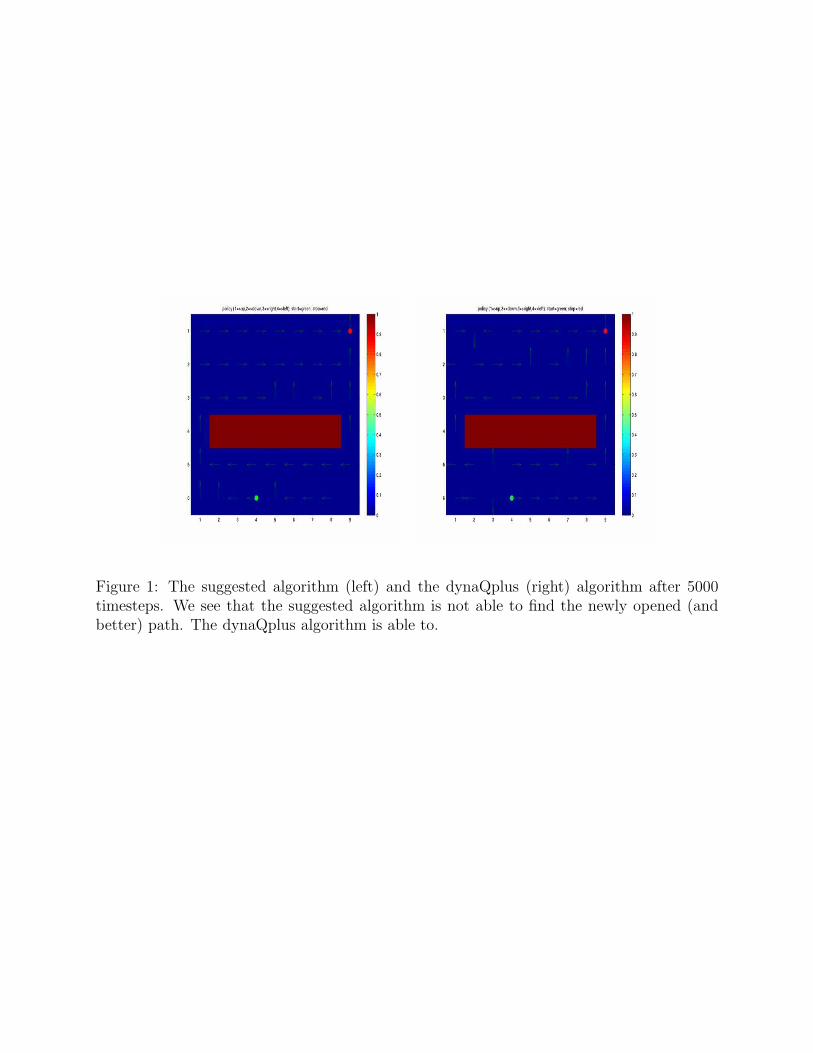
Figure 1: The suggested algorithm (left) and the dynaQplus (right) algorithm after 5000timesteps. We see that the suggested algorithm is not able to find the newly opened (andbetter) path. The dynaQplus algorithm is able to.