solvency capital requirement (scr) for market risks942698/fulltext01.pdf · degree project in...

IN DEGREE PROJECT TECHNOLOGY,FIRST CYCLE, 15 CREDITS

, STOCKHOLM SWEDEN 2016

Solvency Capital Requirement (SCR) for Market RisksA quantitative assessment of the Standard formula and its adequacy for a Swedish insurance company

BJÖRN WIDING

KTH ROYAL INSTITUTE OF TECHNOLOGYSCHOOL OF ENGINEERING SCIENCES

Solvency Capital Requirement (SCR) for

Market Risks

A quantitative assessment of the Standard formula and its adequacy for a Swedish insurance company

B J Ö R N W I D I N G

Degree Project in Applied Mathematics and Industrial Economics (15 credits) Degree Progr. in Industrial Engineering and Management (300 credits)

Royal Institute of Technology year 2016 Supervisors at KTH: Fredrik Armerin, Jonatan Freilich

Examiner: Henrik Hult

TRITA-MAT-K 2016:29 ISRN-KTH/MAT/K--16/29--SE Royal Institute of Technology SCI School of Engineering Sciences KTH SCI SE-100 44 Stockholm, Sweden URL: www.kth.se/sci

AbstractThe purpose of this project is to validate the adequacy of the Standard formula, used

to calculate the Solvency Capital Requirement (SCR), with respect to a Swedishinsurance company. The sub-modules evaluated are Equity risk (type 1) and Interestrate risk. The validation uses a quantitative assessment and the concept of Value atRisk (VaR). Additionally, investment strategies for risk free assets are evaluated

through a scenario based analysis.

The findings support that the Equity shock of -39%, as proposed in the Standardformula, is appropriate for a diversified portfolio of global equities. Furthermore, to

some extent; the Equity shock is also sufficient for a diversified global portfolio with anoverweight of Swedish equities. Additionally, the findings shows that the Standard

formula for Interest rate risks occasionally underestimates the true Interest rate risk.Furthermore, it’s shown that there are some advantage of selecting an investment

strategy that stabilizes the Own fund of an insurance company rather than a strategythat minimizes the SCR.

Keywords:Solvency II, Standard formula, Solvency Capital Requirement, Value at Risk, Principal

Component Analysis, Cornish Fisher expansion

iii

SammanfattningSyftet med detta arbete är att utvärdera Standardformeln, som används för att

beräkna solvenskapitalkravet (SCR) under Solvens II, med avseende på dess lämplighetför ett svensk försäkringsbolag. Modulerna som utvärderas är aktierisk (typ 1) ochränterisk. Utvärderingen genomförs med kvantitativa metoder och utifrån konceptetValue at Risk (VaR). Dessutom utvärderas investeringsstrategier för riskfria tillgångar

genom en scenariobaserad analys.

Resultaten stödjer att den av Standardformeln föreskrivna aktiechocken på -39% ärtillräcklig för en diversifierad global aktieportfölj. Dessutom är aktiechocken även

tillräcklig för en diversifierad global portfölj med en viss övervikt mot svenska aktier.Vidare visar resultaten att Standardformeln under vissa omständigheter underskattarränterisken. Slutligen visar den scenariobaserade analysen att det är fördelaktigt attvälja en investeringsstrategi som stabiliserar Own fund, hellre än en strategi som

minimerar SCR.

Nyckelord:Solvens II, Standardformeln, Kapitalbaskrav, Value at Risk, Principalkomponents

analys, Cornish Fisher expansion

iv

Acknowledgements

SPP

SPP offers saving- and pension solutions to companies, organizations and individuals.The investment focus is especially on sustainability and responsibility. The companyhas a little over 500 employees with head quarter in central Stockholm and is a part of

the Norwegian Storebrand group.

Three people deserve a special mention; they are Fredrik Ehn (actuary), RasmusThunberg (actuarial function) and Fredrik Mases (manager of the actuarial group).

Through this project they and others gave me valuable insights about the life insurancebusiness and the Solvency II regulation. I’m very thankful for their engagement andcontinuous support which made this project viable. Working at the office of SPP was

always a pleasant experience.

Many thanks!/ Björn

v

Contents

Abstract iii

Sammanfattning iv

Acknowledgements v

I Introduction and framework 1

1 Introduction 21.1 Background . . . . . . . . . . . . . . . . . . . . . . . . . . . . . . . . . . . 2

1.1.1 Valuing assets and liabilities . . . . . . . . . . . . . . . . . . . . . . 21.1.2 Solvency Capital Requirement (SCR) . . . . . . . . . . . . . . . . 2

1.2 Objective . . . . . . . . . . . . . . . . . . . . . . . . . . . . . . . . . . . . 31.3 Literature . . . . . . . . . . . . . . . . . . . . . . . . . . . . . . . . . . . . 31.4 Outline of the report . . . . . . . . . . . . . . . . . . . . . . . . . . . . . . 3

2 Preliminaries 52.1 Value at Risk (VaR) . . . . . . . . . . . . . . . . . . . . . . . . . . . . . . 5

2.1.1 Definition . . . . . . . . . . . . . . . . . . . . . . . . . . . . . . . . 52.1.2 Relation to the Quantile function . . . . . . . . . . . . . . . . . . . 52.1.3 Important properties of VaR and the Quantile function . . . . . . 62.1.4 Empirical estimation of VaR . . . . . . . . . . . . . . . . . . . . . 62.1.5 Estimation of VaR using parametric models . . . . . . . . . . . . . 7

2.2 Elliptical distribution . . . . . . . . . . . . . . . . . . . . . . . . . . . . . . 72.3 Principal Component Analysis . . . . . . . . . . . . . . . . . . . . . . . . 8

2.3.1 Principal Component Analysis on shifts in an interest term structure 92.4 Portfolio immunization . . . . . . . . . . . . . . . . . . . . . . . . . . . . . 11

3 Theoretical framework of Solvency II 123.1 Valuing assets and liabilities under Solvency II . . . . . . . . . . . . . . . 12

3.1.1 The risk free interest rate term structure for valuing liabilitiesunder Solvency II . . . . . . . . . . . . . . . . . . . . . . . . . . . . 12

3.2 Solvency Capital Requirement . . . . . . . . . . . . . . . . . . . . . . . . . 133.2.1 The Standard formula . . . . . . . . . . . . . . . . . . . . . . . . . 14

3.3 Implications on the valuation of liabilities and on the SCR for Interestrate risk . . . . . . . . . . . . . . . . . . . . . . . . . . . . . . . . . . . . . 15

vi

3.4 Replication on the Standard formula and the calibration of CEIOPS . . . 163.4.1 Equity risk . . . . . . . . . . . . . . . . . . . . . . . . . . . . . . . 163.4.2 Interest rate risk . . . . . . . . . . . . . . . . . . . . . . . . . . . . 17

II Evaluation of Investment strategies 19

4 Introduction 204.1 Research question . . . . . . . . . . . . . . . . . . . . . . . . . . . . . . . . 214.2 Limitation . . . . . . . . . . . . . . . . . . . . . . . . . . . . . . . . . . . . 21

5 Methodology 225.1 Arranging the portfolios . . . . . . . . . . . . . . . . . . . . . . . . . . . . 22

6 Results 24

7 Discussion and conclusion 26

III A Quantitative Assessment of the Standard formula 28

8 Objective 298.1 Research question . . . . . . . . . . . . . . . . . . . . . . . . . . . . . . . . 298.2 Limitations . . . . . . . . . . . . . . . . . . . . . . . . . . . . . . . . . . . 29

9 Methodology 309.1 Equity risk . . . . . . . . . . . . . . . . . . . . . . . . . . . . . . . . . . . 309.2 Interest rate risk . . . . . . . . . . . . . . . . . . . . . . . . . . . . . . . . 309.3 Data . . . . . . . . . . . . . . . . . . . . . . . . . . . . . . . . . . . . . . . 31

9.3.1 Equity Risk . . . . . . . . . . . . . . . . . . . . . . . . . . . . . . . 319.3.2 Interest rate risk . . . . . . . . . . . . . . . . . . . . . . . . . . . . 31

9.4 Software . . . . . . . . . . . . . . . . . . . . . . . . . . . . . . . . . . . . . 32

10 Results 3310.1 Equity risk . . . . . . . . . . . . . . . . . . . . . . . . . . . . . . . . . . . 3310.2 Interest rate risk . . . . . . . . . . . . . . . . . . . . . . . . . . . . . . . . 37

10.2.1 Modification of the model of relative stresses . . . . . . . . . . . . 3710.2.2 Principal Component Analysis on Swedish interest rates . . . . . . 3910.2.3 Final stress proposals on interest rates . . . . . . . . . . . . . . . . 4210.2.4 Back test . . . . . . . . . . . . . . . . . . . . . . . . . . . . . . . . 44

11 Discussion and conclusion 4811.1 Equity risk . . . . . . . . . . . . . . . . . . . . . . . . . . . . . . . . . . . 4811.2 Interest rate risk . . . . . . . . . . . . . . . . . . . . . . . . . . . . . . . . 49

Bibliography 52

vii

List of Figures

3.1 Market and extrapolated risk free rates per April 1, 2016 . . . . . . . . . 133.2 Comparison of stressed interest rates and stressed extrapolated interest

rates . . . . . . . . . . . . . . . . . . . . . . . . . . . . . . . . . . . . . . . 16

4.1 Extrapolated rates after parallel shifts . . . . . . . . . . . . . . . . . . . . 20

5.1 Illustration of the cash flows from assets and liabilities for the SCR min-imizing portfolio and for the Own fund stabilizing portfolio . . . . . . . . 23

6.1 Own fund and SCR under parallel shifts to the interest rate term structure 24

10.1 Histograms of the yearly returns of OMX30 and MSCI World . . . . . . . 3310.2 QQ-plots of the yearly returns of MSCI World and OMX30 from a daily

rolling window . . . . . . . . . . . . . . . . . . . . . . . . . . . . . . . . . 3510.3 QQ-plots of the yearly returns of S&P and AFGX . . . . . . . . . . . . . 3610.4 Historic changes to GB government lending rates. . . . . . . . . . . . . . . 3710.5 Principal Components . . . . . . . . . . . . . . . . . . . . . . . . . . . . . 3910.6 Histograms of the first and second Principal Values . . . . . . . . . . . . . 4010.7 QQ-plots of the first and second Principal Values . . . . . . . . . . . . . . 4110.8 Shift in risk free term structure between December 3, 2007 and December

3, 2008 . . . . . . . . . . . . . . . . . . . . . . . . . . . . . . . . . . . . . . 4610.9 Shift in risk free term structure between December 10, 2005 and December

10, 2006 . . . . . . . . . . . . . . . . . . . . . . . . . . . . . . . . . . . . . 47

viii

List of Tables

3.1 Interest rate stress factors of the Standard formula . . . . . . . . . . . . . 153.2 Interest rate stresses proposed by EIOPA and Interest rate stresses ob-

tained from a Principal Component analysis on shifts in the term structureof German government lending rates . . . . . . . . . . . . . . . . . . . . . 18

10.1 Statistical properties of the returns from MSCI World, OMX30, S&P andAFGX . . . . . . . . . . . . . . . . . . . . . . . . . . . . . . . . . . . . . . 34

10.2 0.5% quantile of the yearly returns of MSCI World and OMX30 from adaily rolling window . . . . . . . . . . . . . . . . . . . . . . . . . . . . . . 34

10.3 0.5% quantile of the yearly returns of MSCI World and OMX30 from amonthly rolling window . . . . . . . . . . . . . . . . . . . . . . . . . . . . 36

10.4 0.5% quantile of the yearly returns of AFGX and S&P . . . . . . . . . . . 3610.5 Quantiles of the first Principal Component of changes to Swedish zero rates 3810.6 Statistical properties of the first and second Principal Values . . . . . . . 4010.7 Quantiles of the first and second Principal Values . . . . . . . . . . . . . . 4110.8 Proposed stresses to interest rates . . . . . . . . . . . . . . . . . . . . . . 4210.9 Stressed rates per April 1, 2016 . . . . . . . . . . . . . . . . . . . . . . . . 4310.10Empirical left tail of the Own funds stabilizing Portfolio . . . . . . . . . . 4410.11Empirical left tail of the SCR minimizing Portfolio . . . . . . . . . . . . . 4410.12Result from the back test of the Own funds stabilizing portfolio . . . . . . 4510.13Result from the back test of the SCR minimizing portfolio . . . . . . . . . 45

11.1 Comparison of the losses associated to the stress proposed in the Standardformula and the stresses proposed in this thesis . . . . . . . . . . . . . . . 51

ix

Part I

Introduction and framework

1

Chapter 1

Introduction

1.1 Background

The regulation of Solvency II; applying to insurance companies within the EU, wasimplemented January 1, 2016. The regulation is divided into three pillars where Pillar1 determines how an insurance company should value its assets and liabilities, and theminimum capital an insurance company should hold.

1.1.1 Valuing assets and liabilities

As an equivalent to Equity according to the IFRS 1, Solvency II defines the Own fund ofan insurance company which is computed according to the specifications given in Pillar12. The regulation of Solvency II requires that an insurance company holds capital suchthat the Own fund is greater than or equal to the capital requirement. The excess Ownfund defines the Free capital of an insurance company.

1.1.2 Solvency Capital Requirement (SCR)

The capital requirement is computed by either the Standard formula3 or by an internalmodel decided by the insurance company and approved by the responsible authority (inSweden by Finansinspektionen). The Standard formula is a set of stresses on assetsand liabilities; the SCR is computed as the difference between the current value andthe stressed value of the assets and liabilities, i.e. the loss in net value associated withthe stress. The stresses has been defined by EIOPA4 with the objective that the SCRshould be equal to VaR99.5%(Loss) at one year horizon. Specifically, asset and liabilitytypes are divided into groups and subgroups and a SCR is computed for every groupand subgroup, finally; using a correlation matrix the total SCR is computed.

1International Financial Reporting Standards2Hocking et al., 2015.3EIOPA-14/209, 2014.4European Insurance and Occupational Pensions Authority

2

Chapter 1. Introduction

Prior to the calibration of the stresses, CEIOPS 5 made an assessment with thepurpose to estimate the VaR of an average European insurance company. The assessmenthas then been used as a foundation for the calibration of the stresses.

1.2 Objective

The objective of this project is to evaluate investment strategies for risk free assets usingthe framework of Solvency II and financial theory, and to assess the Standard formula onEquity risk (type 1) and Interest rate risk using mathematical and statistical theories.The two objectives are in different parts of the thesis. A more specific motivation of theobjectives are given in Chapter 4 and 8 respectively.

1.3 Literature

The source of literature for this project are mainly the documented assumptions of theStandard formula, the results from the calibration of the Standard formula6, and thetechnical specifications for determining SCR and the risk free term structure7.

Previous work on assessing the Solvency II regulation covers comparisons of theSolvency II regulation with other financial regulations e.g. Basel II/III and the SwissSolvency Test8, and the benefit and drawback for an insurer to develop an internalmodel9. There has also been assessments on some of the sub-modules such as Longevityrisk and Real estate risk10, and on the statistical methods used by EIOPA11. Althoughvery little is found on assessing other markets and market conditions than those assessedby EIOPA, these sources provides a good insight in the Solvency II regulation.

1.4 Outline of the report

Chapter 2 and 3 in this part; presents the mathematical theory and the partial frame-work of Solvency II respectively. The evaluation of investment strategies is presentedin Part II, with a further description of the objectives in Chapter 4, a description ofthe methodology in Chapter 5, a presentation of the results in Chapter 6 and a finaldiscussion and conclusion in Chapter 7. The quantitative assessment of the Standard

5Committee of European Insurance and Occupational Pensions Supervisors (replaced by EIOPA 2011)6EIOPA-14-32, 2014; CEIOPS-SEC-40-10, 2010.7EIOPA-14/209, 2014; EIOPA-BoS-15/035, 2015.8Al-Darwish et al., 2011; Eling, Schmeister, and Schmit, 2006.9Gatzert and Martin, 2012.

10Börger, 2010; Christiansen, Denuit, and Lazar, 2012; Amedee-Manesme and Barthélémy, 2012.11Bauer, Bergmann, and Reuss, 2009; Gatzert and Wesker, 2012; Pfeifer and Strassburger, 2008;

Sandström, 2007.

3


formula that is presented in Part III follows the same pattern, with objectives in Chapter8, methodology in Chapter 9, results in Chapter 10 and a final discussion and conclusionin Chapter 11.

4

Chapter 2

Preliminaries

The mathematical theory collected in this section is mainly from the excellent book Riskand Portfolio Analysis (Hult et al., 2012). Propositions from the book needed for thisthesis are given in this section. For proofs of the propositions, references will be madeto the book.

2.1 Value at Risk (VaR)

2.1.1 Definition

Value at Risk (VaR) at level p is a risk measure that with confidence p is less than thepossible loss L. The mathematical definition used in Solvency II is given by:

VaRp (L) = min {m : P (m < L) ≤ 1− p} (2.1)

2.1.2 Relation to the Quantile function

If L is considered to be a random variable then VaRp(L) is the (p)-quantile function ofL:

VaRp(L) = F−1L (p) (2.2)

where F−1L is defined as;

F−1L (p) = min {m : FL (m) ≥ p} (2.3)

This can be shown by expanding the definition of VaR as follows:

VaRp (X) = min {m : P (m < L) ≤ 1− p} =

= min {m : 1− P (L ≤ m) ≤ 1− p} =

5

Chapter 2. Preliminaries

= min {m : 1− FL (m) ≤ 1− p} =

= min {m : FL (m) ≥ p}

where the last statement equals the definition of the quantile function of L in 2.3.

2.1.3 Important properties of VaR and the Quantile function

From Proposition 6.2 in (Hult et al., 2012) VaR has the properties of Translation invari-ance and of Positive homogeneity meaning that:

VaRp(L+ c) = VaRp(L)− c (2.4)

where c is a constant, andVaRp(λL) = λVaRp(L) (2.5)

where λ is a constant.From proposition 6.3 and 6.4 in (Hult et al., 2012) the quantile function F−1

X has thefollowing important properties:

F−1g(Z) (p) = g

(F−1Z (p)

), (2.6)

if g is a left continuous non-decreasing function, and

F−1−X (p) = −F−1

X (1− p) (2.7)

Consequently, if g is a right continuous non-increasing function then −g is left continuousnon-decreasing which implies that:

F−1g(Z) (p) = −F−1

−g(Z) (1− p) = g(F−1Z (1− p)

)(2.8)

2.1.4 Empirical estimation of VaR

In the common case, the true VaR is unknown and one is therefore forced to makeestimations. Empirical VaR is a method where no assumptions about parametric distri-butions are made, instead VaR is estimated from the outcomes l1 . . . ln.

From the definition of the Quantile function in 2.3, the empirical Quantile functioncan be stated as:

F−1n,L (p) = L[n(1−p)]+1,n (2.9)

where L1,n . . . Ln,n are random variables ordered such that L1,n ≥ . . . ≥ Ln,n and[n (1− p)] = max {m : m < n (1− p)}. Using 2.2 and 2.9 the empirical VaR is as follows:

VaRp (L) = F−1n,L (p) = L[n(1−p)]+1,n (2.10)

6


Thus, the estimated empirical VaR is:

V̂aRp (L) = l[n(1−p)]+1,n (2.11)

where l1,n . . . ln,n are outcomes from L1,n . . . Ln,n, ordered such that l1,n ≥ . . . ≥ ln,n.

2.1.5 Estimation of VaR using parametric models

Contrary to Empirical VaR; when estimating VaR using a parametric model one assumesthat the outcomes l1 . . . ln, are outcomes from a known distribution. With this assump-tion follows that the Quantile function is known. Hence, by estimating the parametersθ of the parametric model function and using 2.2, the estimation of VaR is:

V̂aRp (L) = F−1L,θ̂

(p). (2.12)

Estimation of VaR using Cornish Fisher expansion

If VaR is to be estimated from data with higher order moments, i.e. where E [Xn] forn > 2 departs significantly from zero; then the normal distribution provides a poor fitto the data since the parameters of the normal distribution model only affects the firstand second order moments, i.e. mean and mean square. A remedy in such case is touse Cornish Fisher expansion1 to calibrate for higher order moments. The estimatedVaRp(X), calibrated for moment three and four with Cornish Fisher expansion is;

VaRp(L) ≈ µL + σL

(z + 1

6(z2 − 1)S + 124(z3 − 3z)(K − 3)− 1

36(2z3 − 5z)S2)

(2.13)

where z = Φ−1(p), µL = E [L], σ2L = Var(L), and where S is the Skewness and K − 3

the Excess kurtosis defined as:

S = E[(

X − µXσX

)3]

(2.14)

K − 3 =E[(X − µX)4

](E[(X − µX)2

])2 − 3 (2.15)

2.2 Elliptical distribution

Elliptical distributions are a special case of multivariate distributions. If the lossesL1 . . . Ln of n different assets and liabilities have an elliptical distribution with zero

1Amedee-Manesme and Barthélémy, 2012; Sandström, 2007.

7


mean, then VaR of the total loss of a portfolio consisting of the different assets andliabilities can be computed as follows2:

V aRp

(n∑i=1

Li

)=

√√√√ n∑i=1

n∑j=1

V aRp (Li)V aRp (Lj) ρ (Li, Lj) (2.16)

where ρ (Li, Lj) is the correlation between Li and Lj .

From pp. 274-278 in (Hult et al., 2012); a random vector Y is said to have a sphericaldistribution if OY d= Y, where O is an orthonormal matrix meaning the OOT = I.Furthermore, a random vector X is said to have an elliptical distribution if there existsa matrix A and a spherical distributed variable Y such that X d= µ + AY.

It is shown in (Hult et al., 2012), that if a vector Y ∈ Nd (0, I), then Y has a sphericaldistribution. Consequently, if a vector X ∈ Nd(µ,Σ), then X has a spherical distribu-tion; since

X d= µ + AY

where AAT = Σ.

2.3 Principal Component Analysis

From pp. 74-75 in (Hult et al., 2012); a Principal Component Analysis is an approach inwhich a random vector v ∈ Rn is broken down into n component vectors. This is doneby a linear transformation of v into v∗, such that the elements of v∗ are uncorrelatedwith each other.

Firstly, recall that a covariance matrix is positive semi-definite and hence can be ex-pressed as; Cov (v) = ODOT, where D is a diagonal matrix with non-negative eigenval-ues λ1, . . . , λn of Cov (v) and O is an orthonormal matrix, i.e. OTO = I, whose columns{o1 . . .on} are eigenvectors of Cov (v). The eigenvalues and the eigenvectors may be as-sumed to be ordered such that the diagonal elements of D appear in descending order,i.e. λ1 ≥ . . . ≥ λn.

Secondly, define v∗ as;v∗ = OT (v− E [v]) (2.17)

then the covariance matrix of v∗ is;

Cov (v∗) = E[OT (v− E [v]) (v− E [v])TO

]= OTCov (v)O = D

2Bauer, Bergmann, and Reuss, 2009.

8


which shows that the elements of v∗ are uncorrelated with each other and has variancesλ1, . . . λn.

Lastly, solving for v in 2.17 yields:

v = E [v] + Ov∗. (2.18)

This shows that v can be expressed in terms of the columns ofO times the correspondingelements of v∗. The Principal Components of v are defined by the columns of O, i.e.{o1 . . .on}. The Principal Values of v are defined by the variances of the {v∗

1 . . . v∗n},

i.e. {λ1 . . . λn}.

Furthermore, the total variance of v is:n∑i=1

λi (2.19)

And the variance explained by the j:th Principal Component is thus:

λj∑ni=1 λi

(2.20)

2.3.1 Principal Component Analysis on shifts in an interest term struc-ture

In a general manner, a Principal Component Analysis on shifts in an interest termstructure can be obtained by assuming that;

vk =(vk1 . . . v

kn

)T=(f(∆rk1 , rk−1

1 ) . . . f(∆rkn, rk−1n )

)T(2.21)

are outcomes from v, where ∆rk1 = rkj − rk−1j , and where rk−1

j and rkj are the rateswith maturity j at time k − 1 and k respectively. The function f can be appropriatelyselected, for example if the relative shifts are to be analyzed then;

f(∆rkj , rk−1j ) =

∆rkjrk−1j

while if the absolute shifts are to be analyzed then;

f(∆rkj , rk−1j ) = ∆rkj

9


Since vk1 = f(∆rk1 , rk−11 ), ∆rkj can be expressed in terms of rk−1

j and vkj , i.e.

∆rkj = ∆rkj (rk−1j , vkj )

Thus, the shift for all maturities ∆rk can be expressed as:

∆rk = ∆rk(rk−1,vk

)(2.22)

Using 2.17; for each outcome vk from v; there is a corresponding outcome v∗k from v∗.Hence, using 2.18; ∆rk can instead be expressed in terms of rk−1 and v∗k,

∆rk = ∆rk(rk−1,v∗k

)(2.23)

since E[v] and O are constant vectors.

Consider an interest rate term structure r0 and a portfolio at time 0. If the loss Lof the portfolio is dependent on the shift ∆r(r0,v∗) in the interest rate term structure;then, since r0 is known, the loss only depends on the outcome of v∗. Furthermore,the loss Lj caused by the shift ∆rj(r0, v

∗j ) from the j:th Principal Component can be

expressed as:Lj = hj

(∆rj(r0, v

∗j ))

= gj(v∗j )

From 2.2, 2.6 and 2.8; if gj(v∗j ) is a left continuous non-decreasing function, then;

VaRp(Lj) = gj

(F−1v∗j

(p))

= hj

(∆rj

(r0, F

−1v∗j

(p)))

(2.24)

and if gj(v∗j ) is a right continuous non-increasing function, then;

VaRp(Lj) = gj

(F−1v∗j

(1− p))

= hj

(∆rj

(r0, F

−1v∗j

(1− p)))

(2.25)

Thus, if the above holds; from 2.21, VaRp(Lj) can be estimated by extracting the change∆ri to the rate with maturity i for i = 1 . . . n as follows:

f(∆rki , rk−1i ) = E[f(∆rki , rk−1

i )] + oj,iF̂−1v∗j

(p) (2.26)

in the case where gj is left continuous non-decreasing, and

f(∆rki , rk−1i ) = E[f(∆rki , rk−1

i )] + oj,iF̂−1v∗j

(1− p) (2.27)

in the case where gj is right continuous non-increasing.

10


2.4 Portfolio immunization

Portfolio immunization refers to a match of the durations of assets and liabilities. Theinterpretation of a match in durations is that the value of the assets and the value ofthe liabilities remains equal to each other under a parallel shift in the interest termstructure, i.e. an equal shift to all rates. The value P and the duration D of a portfolioof liabilities are computed as follow:

P (r) =n∑i=0

cie−riti (2.28)

D(P,∆r) = −∇P (r)T∆rP (r) (2.29)

where ci is the cash flow at time ti and ri the rate to time ti.

By solving the Immunization equation pp. 72 (Hult et al., 2012); an asset portfoliothat consists of hj positions of bonds with duration Dj and hk positions of bonds withduration Dk will match the duration of the portfolio of liabilities. The Immunizationequation which is an interpretation of 2.28 and 2.29, can be written as follows:

(Pj PkPjDj PkDk

)(hjhk

)=(PD

)(2.30)

where Pj and Pk are the current prices of the bonds with durationDj andDk respectively.

The solution of the equation is thus:(hjhk

)= 1PjPk(Dk −Dj)

(PkP (Dk −D)PPj(D −Dj)

)(2.31)

11

Chapter 3

Theoretical framework ofSolvency II

This chapter covers the partial framework of Pillar 1 in Solvency II needed for thisproject. That is; the framework for valuing assets and liabilities and determine the Ownfunds, and; the framework for computing SCR on Equity risk (type 1) and Interest raterisk.

3.1 Valuing assets and liabilities under Solvency II

Under the Solvency II principle, Own funds (BOF) is the measure of importance whenevaluating the financial health of an insurance company. Similarly to Shareholders’equity under IFRS, Own fund is determined by:

BOF = Value of assets−Value of liabilities (3.1)

However, the framework for determine the value of assets and the value of the liabilitiesdiffers from IFRS.

According to the Solvency II framework: Assets are valued through their marketvalue. And liabilities are valued by the Best estimate principle; meaning that the lia-bilities are valued as the present value of probability weighted future cash flows, takingcustomer behavior and biometric factors into account. Thus, the best estimate shall cor-respond to the expected present value of future cash-flows required to settle the insuranceobligations.

3.1.1 The risk free interest rate term structure for valuing liabilitiesunder Solvency II

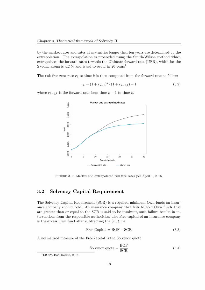
The risk free zero rates used for valuing the expected future cash flows of liabilities isdetermined by a combination of market rates and rates obtained by an extrapolation(Figure 3.1). Specifically for Sweden, rates at maturities up to ten years are determined

12

Chapter 3. Theoretical framework of Solvency II

by the market rates and rates at maturities longer then ten years are determined by theextrapolation. The extrapolation is proceeded using the Smith-Wilson method whichextrapolates the forward rates towards the Ultimate forward rate (UFR), which for theSweden krona is 4.2 % and is set to occur in 20 years1.

The risk free zero rate rk to time k is then computed from the forward rate as follow:

rk = (1 + rk−1)k · (1 + rk−1,k)− 1 (3.2)

where rk−1,k is the forward rate form time k − 1 to time k.

-1.0

0%

0.0

0%

1.0

0%

2.0

0%

3.0

0%

4.0

0%

0 5 10 15 20 25 30

Yiel

d

Term to Maturity

Market and extrapolated rates

Extrapolated rate Market rate

Extrapolated rates after a shift

Figure 3.1: Market and extrapolated risk free rates per April 1, 2016.

3.2 Solvency Capital Requirement

The Solvency Capital Requirement (SCR) is a required minimum Own funds an insur-ance company should hold. An insurance company that fails to hold Own funds thatare greater than or equal to the SCR is said to be insolvent, such failure results in in-terventions from the responsible authorities. The Free capital of an insurance companyis the excess Own fund after subtracting the SCR, i.e.

Free Capital = BOF− SCR (3.3)

A normalized measure of the Free capital is the Solvency quote

Solvency quote = BOFSCR (3.4)

1EIOPA-BoS-15/035, 2015.

13


3.2.1 The Standard formula

As previously mentioned, the Standard formula is a set of stresses which attempt tocapture various risks. The risks are divided into modules and sub-modules. For eachrisk, an SCR specific to the risk is computed. The total SCR of an insurance company isthen computed with the Square root formula, with the assumption that the losses fromeach risk have an elliptical distribution.

SCRTot =

√√√√ n∑i=1

n∑j=1

SCRi · SCRj · ρ (Li, Lj) (3.5)

Equity risk

The capital requirement for Equity risk, SCReq; is determined as the loss L in Own fundafter an Equity shock2.

SCReq = max (L|Equity shock, 0) (3.6)

Formula 3.6 ensures that the SCR is non-negative. For equities (type 1) the Equityshock is -39% plus a symmetrical adjustment.

Interest rate risk

The capital requirement for Interest rate risk; SCRint is determined by computing themaximum loss in Own fund under an upward and a downward stress to risk free interestrates3.

SCRint = max (LUp, LDown, 0) (3.7)

where LUp and LDown are the losses corresponding to the upward and the downwardstress respectively.

The upward stressed rate rUpk and the downward stressed rate rDownk to k years are

determined by relative stress factors as follows:

rUpk = max((1 + sUpk ) · rk, rk + 1%

)(3.8)

rDownk = min

((1 + sDown

k ) · rk, rk)

(3.9)

2EIOPA-14/209, 2014.3EIOPA-14/209, 2014.

14


Table 3.1: Interest rate stress factors of the Standard formula.

k sUpk

sDownk

1 75% −70%2 65% −70%3 56% −64%4 50% −59%5 46% −55%

6 42% −52%7 39% −49%8 36% −47%9 33% −44%

10 31% −42%

11 30% −39%12 29% −37%13 28% −35%14 28% −34%15 27% −33%

16 28% −31%17 28% −30%18 28% −29%19 29% −27%20 29% −26%

where sUpk and sDownk are the relative stress factors shown in Table 3.1 and rk is the

present rate to k years. This has the interpretation that the upward stressed rates areat least 100 basis points over the current rates, and that the downward stressed ratesare the same as the current rates when the current rates are negative, i.e. in times withnegative rates there is no downward stress.

3.3 Implications on the valuation of liabilities and on theSCR for Interest rate risk

As shown in Section 3.1, liabilities maturing after ten years are valued by rates obtainedwith the Smith-Wilson method. Additionally, the SCR on Interest rate risk is derivedfrom a stress that applies to every maturity in the risk free interest rate term structure(Section 3.2.1). The contradiction of the framework is that an actual shift results in anextrapolated risk free term structure while the shift considered for computing SCR isnot extrapolated.

The contradiction is illustrated in Figure 3.2, which displays a hypothetical eventwhere the risk free term structure experiences the same shift as the interest rate stressdefined in the Standard formula. Firstly, it’s worth to notice that the negative rates arenot stressed downwards and that the upward stressed rates are strictly parallel to and100 base points over the rate of April 1, 2016. Secondly, it’s clearly illustrated that therates for determine the SCR does not correspond to the rates that determines the valueof the liabilities after a shift. Consequently, there is a contradiction between hedgingagainst losses in liabilities and hedging with the purpose of minimizing the SCR.

15


Initial rates

-1.0

0%

0.0

0%

1.0

0%

2.0

0%

3.0

0%

4.0

0%

5.0

0%

0 5 10 15 20 25

Yiel

d

Term to Maturity

Extrapolated rates after a shift

Stress Up Stress Down Initial rates

Figure 3.2: Grey line: Risk free rates per April 1, 2016 (with extrapo-lation after ten years). Solid blue and red lines: Stressed rates accordingto the Standard formula. Dashed blue and red lines: Extrapolated ratesafter a hypothetical shift equal to the upward and downward stresses

proposed in the Standard formula, i.e. extrapolated stressed rates.

3.4 Replication on the Standard formula and the calibra-tion of CEIOPS

To capture VaR at one year horizon, any gain or loss expected for the coming year shouldbe included. However, the Standard formula is simplified by proposing instant stresses.Further, through the use of the Square root formula to compute the total SCR, it isassumed that gains and losses have an elliptical distribution.

3.4.1 Equity risk

The calibration of the Equity stress of CEIOPS was derived by estimating the Normalquantile of the return of the index MSCI World at 0.5%. Thus, it’s assumed that thereis no risk from change in volatility on the equity markets. Specifically, the yearly returnsfrom a rolling daily window was used to estimate the parameters of the normal distri-bution function through the Maximum likelihood method.

Mathematically, (using 2.2 and 2.8 in Section 2.1) VaR of the loss L from equities isestimated through the Standard formula under the assumption that

L = g (Re)

16


where g is a right continuous non-increasing function and Re is the equity return. Thus;

VaR99.5% (L) = g(F−1Re

(0.5%))

= L|F−1Re

(0.5%)

= max(L|F−1

Re(0.5%), 0

)= SCR

where the last equality holds if F−1Re

(0.5%) = Equity shock.

For a portfolio exposed to Equity risk from long positions in stocks only, g is clearlyright continuous non-increasing, since the portfolio value V1 at time t1 can be expressedin terms of the return Re and the present value of the portfolio V0, i.e. V1 = V0(1 +Re).Using 2.5 and 2.7 in Section 2.1.3.

VaR99.5% (V0 − V1) = VaR99.5% (V0 − V0(1 +Re)) =

= VaR99.5% (−V0Re) = −V0F−1Re

(0.5%) = L|F−1Re

(0.5%) =

= max(Loss|F−1

Re(0.5%), 0

)= SCR

if F−1Re

(0.5%) = Equity shock.

3.4.2 Interest rate risk

The calibration of the risk free interest rate stresses, performed by CEIOPS was derivedfrom a Principal Component Analysis on the relative change to interest rates. Thus,assuming that the magnitude of shifts in the risk free term structure is proportional tothe level of the rates. Recall Section 2.3.1; the analysis of CEOPS was performed byselecting fj(∆rj) in 2.21 as:

fj(rj ,∆rj) = ∆rjrj

The Principal Component Analysis was performed on German and British governmentlending rates, and on German and British swap rates. Although (CEIOPS-SEC-40-10, 2010) doesn’t contain information about the exact derive of the rate stresses, similarstresses can be derived from the first Principal Component of relative changes in Germangovernment lending rates (Table 3.2). Specifically, the stresses in Table 3.2 are derivedfrom using 2.26 and 2.27 in Section 2.3.1, where the quantiles are 0.25% and 99.75% andthe distribution function is the estimated normal distribution function.

Mathematically, through defining stresses from the first Principal Component; it isassumed that the loss L from shifts in the risk free term structure can be stated as afunction of the first Principal Component v∗

1:

L = g(v∗1)

17


Table 3.2: Interest rate stresses proposed by EIOPA and Interest ratestresses obtained from a Principal Component analysis on shifts in the

term structure of German government lending rates.

EIOPA German rates

1 75% −70% 74% −64%2 65% −70% 77% −69%3 56% −64% 73% −68%4 50% −59% 68% −65%5 46% −55% 63% −61%

6 42% −52% 57% −57%7 39% −49% 53% −53%8 36% −47% 49% −50%9 33% −44% 45% −47%

10 31% −42% 42% −44%

11 30% −39% 39% −42%12 29% −37% 37% −40%13 28% −35% 35% −38%14 28% −34% 33% −36%15 27% −33% 31% −35%

16 28% −31% 30% −33%17 28% −30% 29% −32%18 28% −29% 28% −31%19 29% −27% 27% −30%20 29% −26% 26% −30%

As the SCR is computed from the maximum loss from an upward and a downward shift(3.7 in Section 3.2.1); through 2.2, 2.6 and 2.8 in Section 2.1 it holds that;

SCR = VaR99.5%(L) = g(F−1v∗1

(0.5%))

if g is right continuous non-increasing, and;

SCR = VaR99.5%(L) = g(F−1v∗1

(99.5%))

if g is left continuous non-decreasing.

In the common case where the sensibility of a portfolio to interest rates is only throughfixed cash flows:

L =n∑i=0

ci

(1 + ri + ∆ri(ri, v∗1))i−

n∑i=0

ci

(1 + ri)i

It’s worth to notice that in this case there is no guarantee that g is either left continuousnon-decreasing, or right continuous non-increasing.

18

Part II

Evaluation of Investmentstrategies

19

Chapter 4

Introduction

In the framework of Solvency II there are contradictions in how to value liabilities anddetermine the Solvency Capital Requirement for interest rate risk (SCR) (Section 3.1,3.2.1 and 3.3). That is, the SCR is determined by the net loss caused by proposed shiftsto all risk free rates1, while the present value of the liabilities is determined from a termstructure of market rates up to ten years and extrapolated rates after ten years2. Theimplication of the later is that shifts in market rates mainly affect rates up to ten years.This is illustrated in Figure 4.1, which shows the extrapolated term structure of April 1,2016 and term structures after hypothetical parallel shifts to the market rates at -100,-50, +50 and +100 base points respectively.

-2.0

0%

-1.0

0%

0.0

0%

1.0

0%

2.0

0%

3.0

0%

4.0

0%

0 5 10 15 20 25 30

Yiel

d

Term to Maturity

Scenarios

-100bp -50bp 0 +50bp +100bp

Figure 4.1: Extrapolated rates per April 1, 2016 and after parallel shifts

For life insurance companies that commonly have liabilities with very long durations;the net loss from a parallel shift to all rates (which determines the SCR), and the net lossfrom a parallel shift only for rates up ten years (which affects the value of the liabilities),differs significantly. Thus, for an insurance company that aims to have a stable and andadequate Free capital; a question raised is whether to select an investment strategy for

1EIOPA-14/209, 2014.2EIOPA-BoS-15/035, 2015.

20


risk free assets that stabilizes the Own funds, or a strategy that minimizes the SCR (ora combination of the two).

Basse and Friedrich, 2008 argues that with the imposition of Solcency II, the invest-ment behaviors of insurance companies regarding risk free assets are likely to shift infavour for a strategy that minimizes the SCR. Specifically, they argue that the demandof insurance companies for bonds with long durations will increase; as the insurancecompanies starts to hedge its liabilities against parallel shifts in the term structure forall maturities, in order to minimize the SCR. Contrary, the same research finds no signsof such shift in behavior. Due to the recent introduction of Solvency II, it is reasonableto assume that the there are contrary beliefs within the insurance business of whichstrategy to prefer.

4.1 Research question

The question addressed in this part is if there are significant benefits or drawbacks ofthe strategies discussed above. The research will attempt to find the implications of thestrategies on Own funds and SCR, and in extension on Free capital.

4.2 Limitation

The selection of an investment strategy is a delicate question as the total SCR of aninsurance company is computed from the Square root formula, which accounts for cor-relations between various risks (3.5 in Section 3.2.1). This research will, however; belimited to interest rate risks, excluding the extending effects on the SCR for other risks.One could think of it as a simplified insurance company that only invests in risk freeassets and only have fixed cash flow from its liabilities.

21

Chapter 5

Methodology

Using the theoretical framework of Solvency II (Chapter 3) and especially the theorycaptured in Section 3.1, 3.2 and 3.3 combined with financial theory; the investmentstrategies will be investigated through a scenario based analysis. Four scenarios will beconsidered; a parallel shift to the risk free term structure downwards at 50 and 100 basepoints respectively, and a parallel shift to the risk free term structure upwards at 50 and100 base point respectively (Figure 4.1). I.e. parallel shifts of the risk free term structurewith -1, -0.5, +0.5 and +1 percentage points. The base case is the extrapolated risk freeterm structure of April 1, 2016. The scenarios of parallel shifts are chosen, since themain variation of the risk free interest rate term structure is explained by parallel shifts(CEIOPS-SEC-40-10, 2010) and Section 10.2.2.

Due to the confidentiality of insurance companies, real portfolios can’t be inves-tigated. Instead, hypothetical portfolios of assets and liabilities are constructed, suchthat the portfolios corresponds to the strategies discussed in previous chapter (and linearcombination of the strategies). The portfolios are constructed through the Immuniza-tion equation (2.30 in Section 2.4), which is commonly used by insurance companiesand other investors in order to implement hedging strategies. The exact method forconstructing the portfolios is described in Section 5.1.

For each scenario, the extrapolation proposed by EIOPA1, is proceeded using theSmith-Wilson risk free interest rate extrapolation tool, available at the website of EIOPA.From the extrapolated rates, the value of the portfolios are computed. Furthermore, foreach scenario; the SCR of the portfolios are computed through 3.7 (Section 3.2.1). Thecalculations are made with MS Excel which is a commonly used program for calculations.

5.1 Arranging the portfolios

The portfolios are arranged under the assumption that an insurance company has anegative cash flow from liabilities that declines over time. Furthermore, it is assumed

1EIOPA-BoS-15/035, 2015.

22

Chapter 5. Methodology

that the maturity of the cash flows spans from one to thirty years. For simplicity, thecash flow maturing in one year is selected to 1.0.

On the market, it is assumed that there are bonds available that matures in 0 yearsand in 10 years. From the Immunization equation: Weights of the bonds can be selectedfor a bond portfolio such that the bond portfolio matches the duration and the presentvalue of the liability portfolio. The implication of matching the duration of the port-folios is that the combined value of the bond portfolio and the portfolio of liabilities isinsensitive to parallel shifts in the interest term structure.

The cash flows from the portfolios are shown in Figure 5.1. As shown the hedgeagainst parallel shifts up to thirty years (the SCR minimizing strategy) is obtainedthrough a short positions in bonds maturing in 0 year, and consequently; a larger longposition in bonds maturing in 10 years.

-50

51

01

52

02

5

0 5 10 15 20 25 30Term to maturity

Strategy for stabilizing Own fund

Cashflow from liabilities Cashflow from riskfree assets

-50

51

01

52

02

5

0 5 10 15 20 25 30Term to maturity

Strategy for minimizing SCR

Figure 5.1: Illustration of the cash flows from assets and liabilities forthe SCR minimizing portfolio (upper plot) and for the Own fund stabi-

lizing portfolio (lower plot).

The combined net value of the bond portfolio and the portfolio of liabilities is indeed0 for both cases. For a better illustration of the results, cash equals 5% of the presentvalue of the liabilities is therefore added to both portfolios.

23

Chapter 6

Results

Figure 10.11 shows the behavior of Own fund and SCR under the parallel shifts in therisk free term structure. One should notice that the size of Own fund at base case isequals to the selection of excess cash (5% of the value of the liabilities). Hence, only theslope of the Own fund should be taken into consideration, not the level.

-0.5

0.5

1.5

-100bp -50bp 0 +50bp +100bp

Parallel shift in zero rates

SCR minimizing Portfolio

-0.5

0.5

1.5

-100bp -50bp 0 +50bp +100bp


40% SCR minimizing Portfolio and 60% Own fund stabilizing Portfolio

-0.5

0.5

1.5

-100bp -50bp 0 +50bp +100bp



SCR Own fund

-0.5

0.5

1.5

-100bp -50bp 0 +50bp +100bp



-0.5

0.5

1.5

-100bp -50bp 0 +50bp +100bp



-0.5

0.5

1.5

-100bp -50bp 0 +50bp +100bp


Own fund stabilizing Portfolio

Figure 6.1: Own fund and SCR under parallel shifts to the interest rateterm structure.

Notable for the SCR minimizing strategy (upper left plot) is that the SCR is low andstable, except when rates shifts downwards more then 50 base points. This is explained

24

Chapter 6. Results

by the fact that negative rates has no SCR stress downwards (Section 3.2.1); at the 100base points downward shift, rates with duration up to eight years are negative. Hence,under the downward stress in the particular scenario; the value of the liability increaseswhile the value of the assets remains approximately the same.

Contrary, the Own fund stabilizing strategy (lower right plot) shows to be very effi-cient for its purpose to stabilize Own fund. Clearly, as the bond portfolio leaning moreagainst the Own fund stabilizing portfolio the Own fund is stabilized. Furthermore,although the SCR is higher with the Own fund stabilizing strategy it’s converges to theSCR of the SCR minimizing portfolio in the case where rates are shifted downwards.Hence, the drawback of higher SCR with the Own fund stabilizing strategy vanishes inthe scenario where rates are shifted downwards.

The objective to achieve a stable adequate Free capital is for these scenarios bestachieved with the strategy where 40% is invested in the SCR minimizing portfolio and60% is invested in the Own fund stabilizing portfolio (upper right plot). However, theSCR can’t be negative (Section 3.2.1); therefore in a scenario where rates are shiftedupwards more then 100 base points, the SCR will stabilize while the Own fund willcontinue to decline.

Worth to notice is also that while the SCR minimizing portfolio closes the stateof insolvent (i.e. where SCR > Own Fund) as the term structure shifts upward, theOwn fund stabilizing portfolio closes the state of insolvent as the term structure shiftdownwards.

25

Chapter 7

Discussion and conclusion

In this research a SCR minimizing strategy and an Own fund stabilizing strategy andcombinations of them, has been investigated on their ability to create a stable adequateFree capital. The strategies has been simplified to a match the duration of the bondportfolio with the duration of all liabilities (SCR minimizing strategy), and a match ofthe duration of the bond portfolio with the liabilities maturing within ten years (Ownfund stabilizing strategy).

The strategies were implemented with the Immunization equation 2.31. The resultsshows that the Own fund could be stabilized very efficiently despite the slack in theextrapolation. The SCR however; couldn’t be minimized in the case were the interestterm structure shifted downwards 100 base points. The failure of the SCR minimizingstrategy derives from the fact that the SCR is not completely determined from proposedparallel shift for all rates. According to Section 3.2.1; as risk free rates declines, thestresses that determine the SCR declines as well. Hence, the theoretical approach ofthe Immunization equation did not completely fulfill its purpose of minimizing the SCR.Therefore, in order to successfully minimize the SCR other methods are needed.

The objective of obtain a stable and adequate Free Capital was best achieved througha bond portfolio with the strategy of stabilizing Own fund, or through a bond portfolioheavy weighted to the strategy of stabilizing Own fund. Contrary, the strategy of mini-mizing SCR had a negative effect on the stability of Free capital, through its destabilizingeffect on Own fund.

The trade off of the strategy is obviously a higher SCR. Consequently, when selectingstrategy an insurance company need to take into consideration how sensible it is to ahigh SCR. In figure 10.11 the level of Own fund at base case was determine as 5% of thevalue of the liabilities. In the case where the percentage is lower the pure strategy ofstabilizing Own fund might lead to a very small or negative Free capital. Hence, in suchcase a combination of e.g. 40% SCR minimizing strategy and 60% Own fund stabilizingstrategy might appear more attractive to an insurance company, while for an insurancecompany with a larger amount of cash the pure Own fund stabilizing strategy mightappear more attractive.

26

Chapter 7. Discussion and conclusion

Additionally, the results shows that the Free Capital were affected differently onupwards shifts and downward shift depending on strategy. Hence, another question totake into consideration is the likely future scenario for risk free rates. The downwardscenario is a scenario were record low rates are shifted further down. Assuming suchscenario is less probable than scenarios of upward shifts, then the Own fund stabilizingportfolio appears to be even more attractive.

In conclusion, there are significant benefits from selecting an investment strategy thatfocus on stabilizing Own fund. Partly this might explain why no evidence was found(Basse and Friedrich, 2008) that support that insurance companies are leaning towardsa strategy where the SCR is minimized.

27

Part III

A Quantitative Assessment of theStandard formula

28

Chapter 8

Objective

For an insurance company that chooses to use the Standard formula, a question raised iswhether the stress levels are appropriate with respect to the specific assets and liabilitiesof the firm. Evaluating the adequacy of the Standard formula is an important part ofthe Own Solvency and Risk Assessment-process (ORSA), which is proposed in Pillar2 of Solvency II and constitutes a essential part of the risk management process of aninsurance company. Additionally, since the assessment of CEIOPS the condition forsome asset types have changed, e.g. with the appearance of negative interest rates.

8.1 Research question

The question addressed in this part is weather the stress levels of EIOPA are valid foran insurance company that is not an “average European insurance company”.

8.2 Limitations

The assessment will be limited to the subgroups Equity risk (type one) and Interest raterisk. Assuming an insurance company takes higher weights of equity in their local marketthan an “average European insurer”; assessing Equity risk by comparing different equitymarkets is of importance. As mentioned above, the appearance of negative interestrates is a new phenomenon that has occurred in the Swedish monetary market after theassessment of CEIOPS. Furthermore, there is no downward stress on negative rates inthe Standard formula. Therefore, an assessment of the Interest rate risk, by investigatethe behavior of interest rates in times with low and negative rates is valuable.

29

Chapter 9

Methodology

9.1 Equity risk

As shown in Section 3.4.1, the model of the Standard formula for estimating VaR isaccurate if an insurance company is sensible to equities through long positions only.Although it’s unlikely the common case; it’s reasonable to assume that an insurancecompany is sensible through long positions in stocks to an extent such that

Loss = g(Re)

where g is a right continuous non-increasing function.

Therefore, the research will be on whether the Equity shock of -39% for equities oftype 1, is an adequate estimation of the 0.5% quantile of the returns from equities oftype 1. The assessment will consider the method used by EIOPA i.e. estimation of thequantile through the yearly returns from a daily rolling window with normal distribu-tion. And on the appropriateness of using the returns of MSCI World for estimating theEquity risk of insurance companies that might be more exposed to local indices.

9.2 Interest rate risk

Although it can not be guaranteed that g is either left continuous non-decreasing, orright continuous non-increasing (Section 3.4.2); it will be assumed that so is the case.The research will firstly be on finding a model that is adequate for both high and lowrates, since the model of relative changes to interest rates is unrealistic for rates closeto 0%. From the new model; interest rate stresses will be calibrated with historicalSwedish interest rates, in order to provide a relevant comparison with respect to aSwedish insurance company. Lastly, the new stresses proposed, and the stresses of theStandard formula; will be back tested by comparing the impact of the stresses on twoportfolios of fixed cash flows with the empirical VaR of the portfolios.

30


The portfolios selected for back testing are the SCR minimizing portfolio, and theOwn fund stabilizing portfolio (Chapter 5). As already argued, both portfolios corre-spond to natural investment strategies of life insurance companies. Specifically, a set ofthe two portfolios will be constructed each day such that the strategies of the portfoliosare obtained, given the interest term structure of the specific date; then the net value ofthe portfolios exactly one year after will be captured. The sets that correspond to theempirical VaR of the portfolios will then be used for evaluating the stresses proposedin the result, and the stresses proposed by EIOPA. I.e. the ability of the stresses toestimate the risk on year ahead will be evaluated.

9.3 Data

9.3.1 Equity Risk

The data for assessing Equity risk are daily last prices of the equity indices MSCI World(1973-2016), and OMX30 (1987-2016) from Bloomberg. MSCI World is an importantindex to assess since it’s a common benchmark for global funds. Additionally, the eq-uity chock was actually determined by the lower normal quantile of the return of theindex. OMX30 contains the return of the 30 largest companies listed on NASDAQ OMXStockholm and is often used as a benchmark for Swedish investors.

Complementary, the American equity index S&P (Standard & Poor’s Composite)and the Swedish equity index AFGX (Affärsvärldens generalindex) are used since bothindices cover over a century of yearly returns. AFGX is available at the website of thenewspaper Affärsvärlden; the exact composition of the index has changed several times1,however; the index provides a good reflection of the returns from the main Swedishequities. S&P is available at the homepage of Robert Shiller. The composition of theindex are american companies of varios sizes. Both S&P and AFGX are less diversifiedthan the global index MSCI World, hence they will mainly be viewed as "local indices"complementing OMX30.

9.3.2 Interest rate risk

The data for assessing Interest rate risk are the EUR and GBP government zero termstructures 2 from Deutsche Bundesbank and Bank of England respectively. Both indicesare available on the websites of the banks mentioned. The indices were used by CEIOPSfor their calibration and are therefore important for comparison. Additionally, Swaprates, i.e. forward rates; for Swedish interests rates available at Bloomberg are used.The Swap rates are recalculated into zero rates using 3.2 in Section 3.1.1.

1Waldenström, 2007.2The lending rates of the German and British governments

31


9.4 Software

For simulation and modeling, the free open source program R will be used because ofthe many features for statistic modeling. Complementary, data basis and calculationswill also be made with MS Excel which is a widely used program for calculation.

32

Chapter 10

Results

10.1 Equity risk

A comparison the returns from the indices MSCI World and OMX30 (Figure 10.1)shows that, unlike MSCI Wold, OMX30 has some very high returns, i.e. a fat right tail.Furthermore there is a much higher frequency of returns around -40% from OMX30 thenfrom MSCI World. Therefore the variance of the returns from OMX30 is higher thanthe variance of the returns from MSCI World. Worth to notice is also the clustering inthe tails which is drawback from using yearly returns from a daily rolling window.

MSCI World

−0.4 −0.2 0.0 0.2 0.4 0.6

0.0

1.0

2.0

3.0

OMX30

−0.5 0.0 0.5 1.0

0.0

1.0

2.0

Normal distribution

Figure 10.1: Histograms of the yearly returns of OMX30 and MSCIWorld from a daily rolling window.

33

Chapter 10. Results

From an analysis of the properties of the data it’s shown that not only does the returnfrom the indices differs in terms of variance, additionally; the returns from OMX30 hasa positive skew while the returns from MSCI World has a negative skew (Table 10.1).Similarly, the return from S&P has a negative skew, while the returns from AFGX has apositive skew. The result on the estimated VaR is thus that an estimation using normaldistribution will overestimate the VaR of the return from OMX30, while the VaR of thereturn from MSCI World will be underestimated. The fact the excess kurtosis of thereturn from OMX30 is lower then the excess kurtosis of the return from MSCI Worldwill further punish OMX30.

Table 10.1: Statistical properties of the returns from MSCI World,OMX30, S&P and AFGX.

MSCI World OMX30 SP AFGX

Expected value 0.08 0.13 0.06 0.10Variance 0.03 0.08 0.03 0.05Skewness -0.21 0.25 -0.35 0.37

Excess kurtosis 0.98 0.38 -0.41 0.31

A method for calibrate the normal distribution for skewness and excess kurtosis isthe Cornish Fisher expansion (Section 2.1.5). The method has previously been used inassessments of the Standard formula1. Additionally, the method is flexible since both itallows for calibration against both positive and negative skewness and excess kurtosis.

Shown in Table 10.2 are the 0.5% quantiles from the empirical estimations, and fromestimations by normal distribution and Cornish Fisher expansion to the third order (cal-ibrated for skewness) and fourth order (calibrated for skewness and excess kurtosis) re-spectively. To achieve a better comparison of the returns from MSCI World and OMX30respectively, and to investigate the robustness of the estimation; samples from differenttime periods has been used for MSCI World. Additionally, returns from a portfolioequally weighted into MSCI World and OMX30 (last column) has been investigated.

Table 10.2: 0.5% quantile of the yearly returns of MSCI World andOMX30 from a daily rolling window.

MSCI World MSCI World MSCI World OMX30 50/50(1973-2009) (1973-2015) (1987-2015) (1987-2015) (1987-2015)

Empirical −44.46% −44.28% −45.15% −44.97% −42.64%Normal −39.27% −37.00% −33.81% −57.68% −42.59%

Cornish Fisher (third order) −42.94% −40.27% −46.33% −51.85% −49.80%Cornish Fisher (fourth order) −47.17% −46.09% −48.13% −54.96% −47.72%

As expected, when calibrating for skewness; the quantiles of the returns from OMX30and MSCI World are closing each other. Worth to notice is also that the empiricalestimations of the quantile at 0.5% of the returns from the two indices and for samplesfrom different time periods are very close to each other. Furthermore, while the normalestimation of the 0.5% quantile of the returns from MSCI World for different time periodsis rather unstable, the Cornish Fisher fourth order estimation is very stable.

1Sandström, 2007.

34

Chapter 10. Results

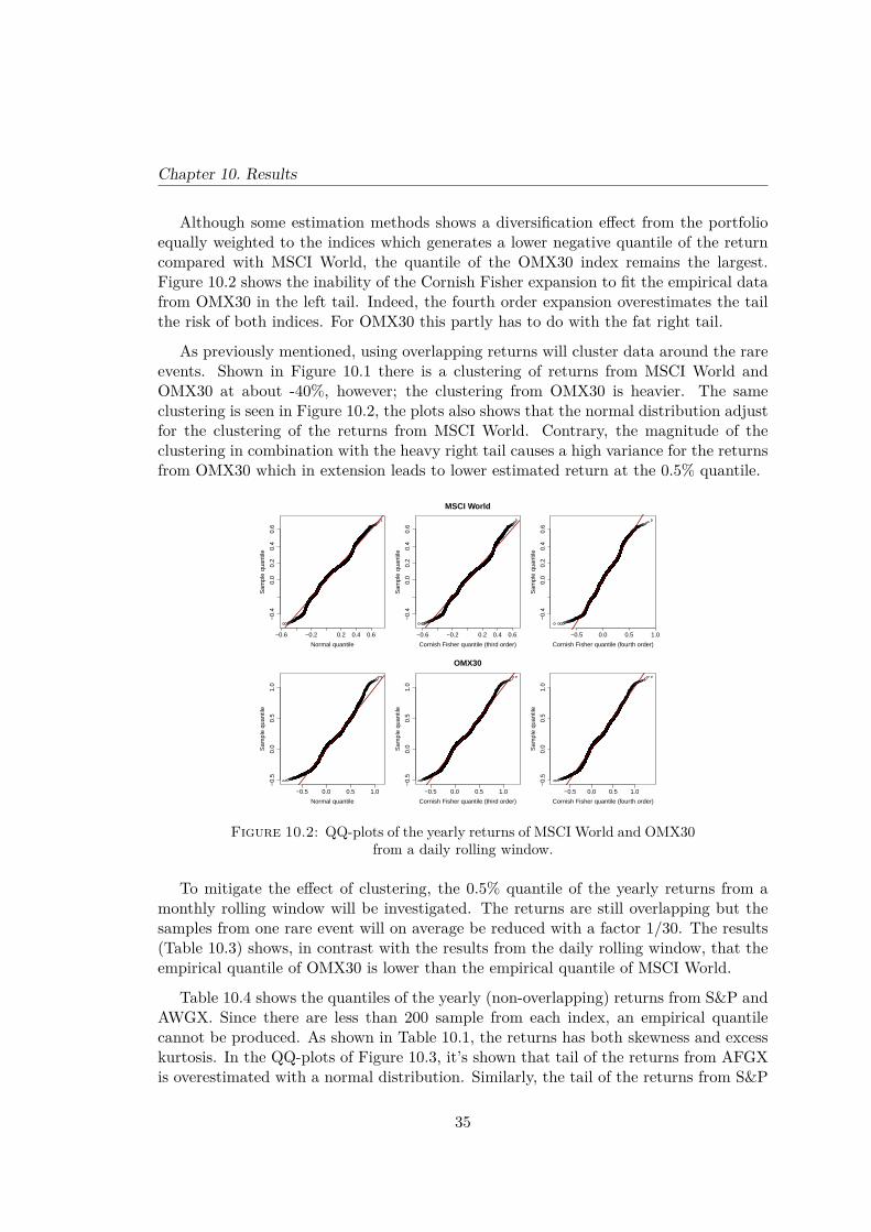
Although some estimation methods shows a diversification effect from the portfolioequally weighted to the indices which generates a lower negative quantile of the returncompared with MSCI World, the quantile of the OMX30 index remains the largest.Figure 10.2 shows the inability of the Cornish Fisher expansion to fit the empirical datafrom OMX30 in the left tail. Indeed, the fourth order expansion overestimates the tailthe risk of both indices. For OMX30 this partly has to do with the fat right tail.

As previously mentioned, using overlapping returns will cluster data around the rareevents. Shown in Figure 10.1 there is a clustering of returns from MSCI World andOMX30 at about -40%, however; the clustering from OMX30 is heavier. The sameclustering is seen in Figure 10.2, the plots also shows that the normal distribution adjustfor the clustering of the returns from MSCI World. Contrary, the magnitude of theclustering in combination with the heavy right tail causes a high variance for the returnsfrom OMX30 which in extension leads to lower estimated return at the 0.5% quantile.

−0.6 −0.2 0.2 0.4 0.6

−0.

40.

00.

20.

40.

6

Normal quantile

Sam

ple

quan

tile

−0.6 −0.2 0.2 0.4 0.6

−0.

40.

00.

20.

40.

6

MSCI World

Cornish Fisher quantile (third order)

Sam

ple

quan

tile

−0.5 0.0 0.5 1.0

−0.

40.

00.

20.

40.

6

Cornish Fisher quantile (fourth order)

Sam

ple

quan

tile

−0.5 0.0 0.5 1.0

−0.

50.

00.

51.

0

Normal quantile

Sam

ple

quan

tile

−0.5 0.0 0.5 1.0

−0.

50.

00.

51.

0

OMX30


Sam

ple

quan

tile

−0.5 0.0 0.5 1.0

−0.

50.

00.

51.

0


Sam

ple

quan

tile

Figure 10.2: QQ-plots of the yearly returns of MSCI World and OMX30from a daily rolling window.

To mitigate the effect of clustering, the 0.5% quantile of the yearly returns from amonthly rolling window will be investigated. The returns are still overlapping but thesamples from one rare event will on average be reduced with a factor 1/30. The results(Table 10.3) shows, in contrast with the results from the daily rolling window, that theempirical quantile of OMX30 is lower than the empirical quantile of MSCI World.

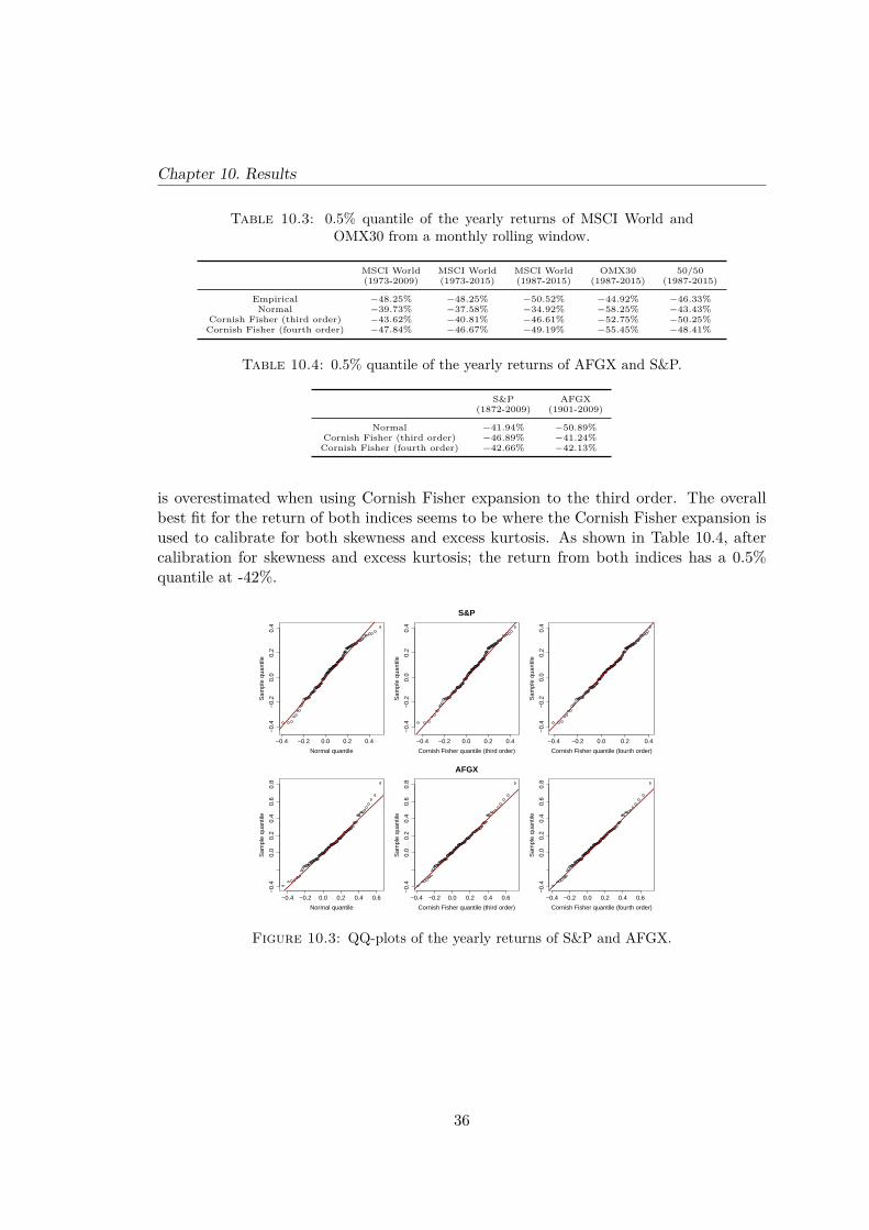
Table 10.4 shows the quantiles of the yearly (non-overlapping) returns from S&P andAWGX. Since there are less than 200 sample from each index, an empirical quantilecannot be produced. As shown in Table 10.1, the returns has both skewness and excesskurtosis. In the QQ-plots of Figure 10.3, it’s shown that tail of the returns from AFGXis overestimated with a normal distribution. Similarly, the tail of the returns from S&P

35

Chapter 10. Results

Table 10.3: 0.5% quantile of the yearly returns of MSCI World andOMX30 from a monthly rolling window.

MSCI World MSCI World MSCI World OMX30 50/50(1973-2009) (1973-2015) (1987-2015) (1987-2015) (1987-2015)

Empirical −48.25% −48.25% −50.52% −44.92% −46.33%Normal −39.73% −37.58% −34.92% −58.25% −43.43%

Cornish Fisher (third order) −43.62% −40.81% −46.61% −52.75% −50.25%Cornish Fisher (fourth order) −47.84% −46.67% −49.19% −55.45% −48.41%

Table 10.4: 0.5% quantile of the yearly returns of AFGX and S&P.

S&P AFGX(1872-2009) (1901-2009)

Normal −41.94% −50.89%Cornish Fisher (third order) −46.89% −41.24%

Cornish Fisher (fourth order) −42.66% −42.13%

is overestimated when using Cornish Fisher expansion to the third order. The overallbest fit for the return of both indices seems to be where the Cornish Fisher expansion isused to calibrate for both skewness and excess kurtosis. As shown in Table 10.4, aftercalibration for skewness and excess kurtosis; the return from both indices has a 0.5%quantile at -42%.

−0.4 −0.2 0.0 0.2 0.4

−0.

4−

0.2

0.0

0.2

0.4

Normal quantile

Sam

ple

quan

tile

−0.4 −0.2 0.0 0.2 0.4

−0.

4−

0.2

0.0

0.2

0.4

S&P


Sam

ple

quan

tile

−0.4 −0.2 0.0 0.2 0.4

−0.

4−

0.2

0.0

0.2

0.4


Sam

ple

quan

tile

−0.4 −0.2 0.0 0.2 0.4 0.6

−0.

40.

00.

20.

40.

60.

8

Normal quantile

Sam

ple

quan

tile

−0.4 −0.2 0.0 0.2 0.4 0.6

−0.

40.

00.

20.

40.

60.

8

AFGX


Sam

ple

quan

tile

−0.4 −0.2 0.0 0.2 0.4 0.6

−0.

40.

00.

20.

40.

60.

8


Sam

ple

quan

tile

Figure 10.3: QQ-plots of the yearly returns of S&P and AFGX.

36

Chapter 10. Results


10.2.1 Modification of the model of relative stresses

In this section, the analysis which aims to make an appropriate selection of f(rj ,∆rj)for the Principal Component analysis (2.21 in Section 2.3.1) is presented. As previ-ously mentioned; the relative change to interest rates will approach infinity as the ratesapproaches zero. This is shown in the middle plot of Figure 10.4; clearly, the relativechange spikes after 2012, as the rates approaches zero.

1980 1990 2000 2010

−6

−2

24

Absolute change in interest rate

1980 1990 2000 2010

−0.

50.

51.

5

Relative change in interest rate

1980 1990 2000 2010

−0.

40.

00.

4

"Relative/absolute mix" change in interest rate

5 year rate 10 year rate 15 year rate

Figure 10.4: Historic changes to GB government lending rates. Upperplot: Absolute change. Middle plot: Relative change. Lower plot: Change

relative to max(rate,4%).

In order to preform a successful Principal Components analysis, a model that is moreconsistent over time is needed. A natural first choice is to replace the model of relativechange with a model of absolute change. However, as seen in the upper plot of Figure10.4; the absolute change to interest rates is in fact higher in times with high rates thanin times with low rates. Indeed, the model of relative change seems reasonable from1980 until 2009.

In order to keep the benefits of the model of relative change and the benefits of themodel of absolute change a "Relative/absolute mix" model is proposed:

f(rj ,∆rj) = ∆rjmax(rj , rfloor)

37

Chapter 10. Results

where rfloor is the lowest possible value of the denominator.

From an ocular review, both the model of relative change and the model of absolutechange in Figure 10.4 seems to be consistent from the year of 2000 until the year of2007. On average the interest rates for different maturities were close to 4% during thespecific period. rfloor is therefore selected to 4% and the final "Relative/absolute mix"model is thus:

f(rj ,∆rj) = ∆rjmax(rj , 4%) (10.1)

As seen in the lower plot of Figure 10.4; with rfloor = 4%, the "Relative/absolute mix"model preforms well both under times with high and low interest rates. Although this ismainly a construction from an ocular review; 4% is indeed close to the Ultimate ForwardRate of 4.2%, which by EIOPA is considered to be the long term average rate2.

Table 10.5: Quantiles of the first Principal Component of changes toSwedish zero rates.

Absolute change Relative change Relative/absolute mix Relative/absolute mix(2001-2007) (2001-2007) (2001-2007) (2001-2015)

1 1.1% −1.5% 92% −75% 48% −38% 47% −56%2 1.6% −1.9% 85% −71% 50% −41% 49% −59%3 1.8% −2.1% 76% −66% 50% −42% 48% −59%4 1.9% −2.3% 69% −61% 50% −43% 47% −58%5 2.0% −2.4% 64% −58% 49% −44% 47% −57%

6 2.0% −2.4% 59% −55% 48% −44% 45% −56%7 1.9% −2.4% 56% −53% 47% −45% 44% −55%8 1.9% −2.4% 53% −51% 46% −45% 43% −54%9 1.9% −2.4% 51% −50% 45% −44% 42% −53%

10 1.9% −2.4% 49% −49% 45% −44% 42% −52%

11 1.8% −2.4% 48% −48% 44% −44% 42% −52%12 1.8% −2.4% 46% −47% 44% −44% 41% −51%13 1.8% −2.4% 45% −47% 43% −44% 41% −51%14 1.8% −2.4% 44% −46% 43% −44% 41% −51%15 1.8% −2.4% 43% −46% 42% −44% 41% −51%

16 1.7% −2.4% 43% −45% 42% −44% 40% −50%17 1.7% −2.4% 42% −45% 41% −45% 40% −50%18 1.7% −2.4% 41% −45% 41% −45% 40% −50%19 1.7% −2.4% 41% −45% 41% −45% 40% −50%20 1.7% −2.5% 40% −44% 40% −45% 40% −50%

21 1.7% −2.5% 40% −44% 40% −45% 40% −50%22 1.7% −2.5% 40% −44% 40% −45% 40% −50%23 1.7% −2.5% 39% −44% 40% −45% 40% −50%24 1.7% −2.5% 39% −44% 40% −45% 40% −50%25 1.7% −2.5% 39% −44% 39% −45% 40% −50%

26 1.7% −2.5% 38% −43% 39% −44% 40% −50%27 1.7% −2.5% 38% −43% 39% −44% 40% −50%28 1.7% −2.4% 38% −43% 39% −44% 40% −50%29 1.7% −2.4% 37% −43% 38% −44% 40% −50%30 1.7% −2.4% 37% −42% 38% −44% 40% −50%

The effect from introducing the "Relative/absolute mix" model to the Principal Com-ponent Analysis is shown in Table 10.5. The table presents the 0.25% and the 99.75%normal quantile of the first Principal Component. A significant difference between theoutcomes of relative changes (column 2) and of the "Relative/absolute mix" model (col-umn 3); is that the shifts derived from the "Relative/absolute mix" model are approx-imately the same for all maturities, while the relative shifts are higher for short rates

2EIOPA-BoS-15/035, 2015.

38

Chapter 10. Results

than for long rates. The Principal Component Analysis on Absolute changes (column 1)shows a similar result, i.e. the shifts are rather the same for all maturities. Tradition-ally short rates has been lower than long rates; it is therefore likely that the differentoutcomes of the models is derived from equal absolute shifts to all maturities, whichmeans higher relative shifts for short rates than for long rates. Hence, it’s reasonable toconclude that the absolute difference between the stressed rates and the current ratesshould be the same for all maturities.

Expanding the time period of the Relative/absolute mix model to 2015 (column 4);shows that the upward shifts are similar, however; the downward shifts increases for allmaturities, which possible can be derived from the downward trend of interest rates from2008. Nevertheless, the "Relative/absolute mix" model shows to be rather robust withrespect to the different time periods.

10.2.2 Principal Component Analysis on Swedish interest rates

In this section, the selection of f(rj ,∆rj) (10.1) in previous section is used to derivestresses on interest rates corresponding VaR0.5%(Loss). Figure 10.5 shows the first fourPrincipal Components derived from Swedish zero rates from 2001 to 2015, using the"Relative/absolute mix" model. The changes are yearly from a daily rolling window.

5 10 15 20 25 30

−0.

4−

0.2

0.0

0.2

0.4

0.6

Principal Components

Term to maturity

Prin

cipa

l Com

pone

nt le

vel

PC 1 PC 2 PC 3 PC 4

Figure 10.5: Principal Components of changes to Swedish zero ratesrelative to max(rate,4%).

39

Chapter 10. Results

As shown, the first Principal Component corresponds to almost equal shifts for allmaturities while the second Principal Component corresponds to shifts in opposite di-rections for long and short rates. The partial contributions of Principal Component oneand two to the total variance of changes to the term structure is 84.6% and 14.4% re-spectively, which makes the combined contribution 99%. Although Principal Componentone has the largest variance, to a life insurance company which can be assume to haveliabilities with long duration; Principal Component two represents shifts that might bemore detrimental. It’s thus reasonable to consider shifts derived from both PrincipalComponent one and two.

Principal Value 1

−2 −1 0 1 2

0.0

0.1

0.2

0.3

0.4

Principal Value 2

−0.5 0.0 0.5 1.0

0.0

0.5

1.0

1.5

Normal distribution

Figure 10.6: Histograms of the first and second Principal Values.

The histograms of Figure 10.6 show the distributions of Principal Value one and two.Worth to notice is that the first Principal Value has a very negative excess kurtosis,and that both Principal Values have a positive skew (Table 10.6). Furthermore, thesecond Principal Value has a clustering of outcomes around 1 which corresponds to alarge downward shift in short rates relative to long rates.

Table 10.6: Statistical properties of the first and second Principal Val-ues.

PV 1 PV 2

Expected value 0.00 0.00Variance 0.85 0.16Skewness 0.22 0.66

Excess kurtosis -1.08 -0.04

40

Chapter 10. Results

The fact that both Principal Values show skewness and excess kurtosis makes theCornish Fisher expansion to the fourth order appropriate for estimating the quantiles.Shown in the QQ-plots in Figure 10.7; a normal distribution will overestimate all quan-tiles except the upper quantile of the second Principal Value. A similar overestimationappears with a Cornish Fisher expansion to the third order. Although the drawback ofinstability in the tail, sometimes inherited from Cornish Fisher expansion, is seen in thelower tails of both Principal Values; Cornish Fisher expansion to the fourth order clearlyprovides the best fit.

−3 −2 −1 0 1 2 3

−1

01

2

Normal quantile

Sam

ple

quan

tile

−3 −2 −1 0 1 2 3

−1

01

2Principal Value 1


Sam

ple

quan

tile

−1 0 1 2−

10

12


Sam

ple

quan

tile

−1.0 −0.5 0.0 0.5 1.0

−0.

50.

00.

51.

0

Normal quantile

Sam

ple

quan

tile

−1.0 −0.5 0.0 0.5 1.0 1.5

−0.

50.

00.

51.

0

Principal Value 2


Sam

ple

quan

tile

−0.5 0.0 0.5 1.0 1.5

−0.

50.

00.

51.

0


Sam

ple

quan

tile

Figure 10.7: QQ-plots of the first and second Principal Values.

Table 10.6 shows the estimated quantiles of the Principal Values. Notable is thatthe Normal distribution and the Cornish Fisher expansions overestimate the empiricalquantile. Worth to notice is that the empirical quantiles are asymmetric which indicatesthat; the largest parallel shifts are downward shifts, and the largest change in curvatureis a decline to short rates against long rates.

Table 10.7: Quantiles of the first and second Principal Values

PV 1 PV 20.5% 99.5% 0.5% 99.5%

Empirical -1.69 1.81 -0.65 1.05Normal -2.36 2.36 -1.00 1.00

Cornish Fisher (third order) -2.17 2.60 -0.77 1.21Cornish Fisher (fourth order) -1.77 2.20 -0.68 1.11

41

Chapter 10. Results

10.2.3 Final stress proposals on interest rates

The stress proposals given in this section are from using

f(rj ,∆rj) = ∆rjmax(rj , 4%)

on 2.26 and 2.27 in Section 2.3.1. Theoretically, the stress proposals are computedfrom the Principal Components, the mean vector (right columns of Table 10.8) and thequantiles of the Principal Values (Table 10.6) using 2.24 in Section 2.3.1. However, thesamples evaluated are from a time period were the interest rates on average fell. As thereare contrary believes on the future drift of interest rates, and since the Standard formulais computed from instant stresses (assuming zero mean); the stresses presented in Table10.8 are computed assuming the mean vector is zero. Additionally to the stress levelsderived from the Cornish Fisher expansion, stresses derived from the normal distributionare also presented.

Table 10.8: Proposed stresses to interest rates for derived from the nor-mal quantile and the quantile from the Cornish Fisher expansion (fourthorder). Left columns: Stresses derived from Principal Component 1.Middle columns: Stresses derived from Principal Component 2. Right

columns: Mean and Principal Component vectors

PC 1 PC 2Normal CF 4 Normal CF 4 PC 1 PC 2 Mean

1 43% −43% 33% −40% 59% −59% 40% −66% −18% −59% −6%2 46% −46% 35% −43% 43% −43% 29% −47% −20% −43% −6%3 47% −47% 35% −44% 30% −30% 21% −34% −20% −30% −7%4 47% −47% 35% −44% 22% −22% 15% −25% −20% −22% −7%5 46% −46% 35% −43% 17% −17% 11% −18% −20% −17% −7%

6 46% −46% 34% −43% 12% −12% 8% −13% −19% −12% −6%7 45% −45% 34% −42% 8% −8% 5% −9% −19% −8% −6%8 44% −44% 33% −41% 5% −5% 3% −5% −19% −5% −6%9 44% −44% 33% −41% 2% −2% 2% −3% −19% −2% −6%

10 43% −43% 32% −40% 0% 0% 0% 0% −18% 0% −6%

11 43% −43% 32% −40% −1% 1% −1% 1% −18% 1% −6%12 43% −43% 32% −40% −3% 3% −2% 3% −18% 3% −6%13 43% −43% 32% −40% −4% 4% −3% 5% −18% 4% −6%14 43% −43% 32% −40% −6% 6% −4% 6% −18% 6% −6%15 42% −42% 32% −40% −7% 7% −5% 8% −18% 7% −6%

16 42% −42% 32% −39% −8% 8% −6% 9% −18% 8% −6%17 42% −42% 32% −39% −9% 9% −6% 10% −18% 9% −6%18 42% −42% 31% −39% −10% 10% −7% 11% −18% 10% −6%19 42% −42% 31% −39% −11% 11% −8% 12% −18% 11% −6%20 42% −42% 31% −39% −12% 12% −8% 13% −18% 12% −6%

21 42% −42% 31% −39% −13% 13% −9% 14% −18% 13% −5%22 42% −42% 31% −39% −13% 13% −9% 14% −18% 13% −5%23 42% −42% 31% −39% −14% 14% −9% 15% −18% 14% −5%24 42% −42% 31% −39% −14% 14% −10% 16% −18% 14% −5%25 42% −42% 31% −39% −15% 15% −10% 16% −18% 15% −5%

26 42% −42% 31% −39% −15% 15% −10% 16% −18% 15% −5%27 42% −42% 31% −39% −15% 15% −10% 17% −18% 15% −5%28 42% −42% 31% −39% −15% 15% −10% 17% −18% 15% −5%29 42% −42% 31% −39% −15% 15% −11% 17% −18% 15% −5%30 42% −42% 31% −39% −16% 16% −11% 18% −18% 16% −5%

42

Chapter 10. Results

For a better comparison of the stresses presented in Table 10.8 with the stressesproposed by EIOPA, the stressed rates computed from the actual rates of April 1, 20163are presented in 10.9.

Table 10.9: Stressed rates per April 1, 2016.

PC 1 PC 2 EIOPA RatesNormal CF 4 Normal CF 4 01/04/16

1 1.19% −2.29% 0.75% −2.17% 1.82% −2.92% 1.06% −3.18% 0.45% −0.55% −0.55%2 1.41% −2.29% 0.95% −2.16% 1.27% −2.15% 0.72% −2.34% 0.56% −0.44% −0.44%3 1.61% −2.13% 1.14% −2.00% 0.96% −1.48% 0.57% −1.61% 0.74% −0.26% −0.26%4 1.82% −1.92% 1.35% −1.79% 0.84% −0.94% 0.56% −1.04% 0.95% −0.05% −0.05%5 2.04% −1.68% 1.57% −1.55% 0.84% −0.48% 0.63% −0.56% 1.18% 0.10% 0.18%

6 2.24% −1.42% 1.78% −1.30% 0.89% −0.07% 0.73% −0.12% 1.41% 0.24% 0.41%7 2.41% −1.19% 1.96% −1.07% 0.93% 0.29% 0.83% 0.26% 1.61% 0.37% 0.61%8 2.55% −0.99% 2.11% −0.87% 0.97% 0.59% 0.91% 0.57% 1.78% 0.50% 0.78%9 2.68% −0.82% 2.24% −0.70% 1.02% 0.84% 0.99% 0.83% 1.93% 0.63% 0.93%

10 2.80% −0.66% 2.37% −0.54% 1.09% 1.05% 1.08% 1.05% 2.07% 0.74% 1.07%

11 2.95% −0.49% 2.52% −0.38% 1.19% 1.27% 1.20% 1.28% 2.23% 0.86% 1.23%12 3.13% −0.31% 2.70% −0.19% 1.31% 1.51% 1.34% 1.52% 2.41% 1.00% 1.41%13 3.30% −0.12% 2.87% −0.01% 1.43% 1.75% 1.48% 1.77% 2.59% 1.14% 1.59%14 3.46% 0.04% 3.03% 0.16% 1.52% 1.98% 1.59% 2.00% 2.75% 1.26% 1.75%15 3.60% 0.20% 3.17% 0.32% 1.61% 2.19% 1.70% 2.23% 2.90% 1.39% 1.90%

16 3.73% 0.35% 3.31% 0.46% 1.71% 2.37% 1.82% 2.41% 3.04% 1.47% 2.04%17 3.84% 0.48% 3.42% 0.59% 1.79% 2.53% 1.91% 2.57% 3.16% 1.56% 2.16%18 3.95% 0.59% 3.53% 0.71% 1.86% 2.68% 1.99% 2.72% 3.27% 1.64% 2.27%19 4.04% 0.70% 3.62% 0.81% 1.92% 2.82% 2.07% 2.86% 3.37% 1.68% 2.37%20 4.12% 0.80% 3.71% 0.91% 1.97% 2.95% 2.13% 3.00% 3.46% 1.75% 2.46%

21 4.20% 0.88% 3.79% 0.99% 2.04% 3.04% 2.20% 3.10% 3.54% 1.81% 2.54%22 4.28% 0.96% 3.87% 1.07% 2.10% 3.14% 2.26% 3.20% 3.62% 1.87% 2.62%23 4.36% 1.02% 3.94% 1.14% 2.15% 3.23% 2.32% 3.29% 3.69% 1.92% 2.69%24 4.42% 1.08% 4.00% 1.20% 2.19% 3.31% 2.37% 3.37% 3.75% 1.97% 2.75%25 4.48% 1.14% 4.06% 1.26% 2.23% 3.39% 2.41% 3.46% 3.81% 2.01% 2.81%

26 4.53% 1.19% 4.11% 1.31% 2.27% 3.45% 2.46% 3.52% 3.86% 2.05% 2.86%27 4.58% 1.24% 4.16% 1.36% 2.31% 3.51% 2.50% 3.58% 3.91% 2.09% 2.91%28 4.62% 1.28% 4.20% 1.40% 2.34% 3.56% 2.54% 3.63% 3.95% 2.13% 2.95%29 4.67% 1.33% 4.25% 1.45% 2.38% 3.62% 2.58% 3.69% 4.00% 2.16% 3.00%30 4.71% 1.37% 4.29% 1.49% 2.41% 3.67% 2.61% 3.74% 4.04% 2.20% 3.04%

The upward stress rates proposed by EIOPA are in this case one unit percent higherthen the rates per 01/04/16 for all maturities. Similarly, since the actual rates are lowerthan 4% for all maturities, the stressed rates derived from the first Principal Componentsare almost parallel to the actual rates. Specifically, the upward stress rates from the firstPrincipal Component are 1.3 unit percent above the actual rates when using the quantileof Cornish Fisher fourth order and 1.7 unit percent above the actual rates when usingthe quantile of normal distribution.

The downward stressed rates derived from the first Principal Component are conse-quently around 1.7 unit percent below the actual rates when using the quantile of thenormal distribution, however; due to the asymmetry of the quantiles from the CornishFisher expansion, the downward stressed rates derived from the Cornish Fisher expan-sion are around 1.6 unit percent below the actual rates. Contrary the downward stressedrates proposed by EIOPA are the same as current rates for short maturities, since thecurrent rates for short maturities are negative; and around 0.6 unit percent below thecurrent rates for long maturities.

3Extrapolated rates proposed by EIOPA (Figure 3.1)

43

Chapter 10. Results

10.2.4 Back test

Table 10.10 and 10.11 shows the left tail of the returns of the Own funds stabilizingportfolio and the SCR minimizing portfolio respectively. As described in Section 5.1;the portfolios were rearranged each day according to the desired strategy and such thatthe net value of the portfolios was zero. Hence, the net values of the portfolios exactlyone year after they were rearranged (last column) equal the loss of the portfolios fromthe previous year.

Table 10.10: Empirical left tail of the absolute yearly return of the Ownfunds stabilizing Portfolio from a daily rolling window

Date Liability value Asset value Net value

16-12-11 14.88 14.03 -0.8516-12-11 14.86 14.03 -0.8301-06-12 15.09 14.27 -0.8215-12-11 14.83 14.02 -0.8101-06-12 15.07 14.27 -0.8013-12-11 14.82 14.04 -0.7808-12-11 14.76 13.98 -0.7806-06-12 15.09 14.32 -0.7813-01-12 14.83 14.06 -0.7701-06-12 15.03 14.27 -0.7714-12-11 14.86 14.10 -0.7718-01-12 14.80 14.04 -0.7601-02-12 14.70 13.94 -0.7620-01-12 14.64 13.89 -0.7504-12-08 14.08 13.33 -0.7503-12-08 14.03 13.28 -0.75

Table 10.11: Empirical left tail of the absolute yearly return of the SCRminimizing Portfolio from a daily rolling window

Date Liability value Asset value Net value

11-06-04 9.95 9.55 -0.4011-06-04 9.94 9.55 -0.3926-08-11 13.10 12.71 -0.3916-06-04 9.97 9.59 -0.3911-06-04 9.93 9.55 -0.3817-06-04 9.93 9.57 -0.3610-06-04 9.94 9.58 -0.3523-09-11 13.42 13.08 -0.3425-08-11 13.02 12.69 -0.3324-10-06 11.07 10.73 -0.3323-09-11 13.41 13.08 -0.3301-07-04 9.98 9.65 -0.3307-07-06 10.84 10.51 -0.3307-06-11 11.82 11.49 -0.3308-06-11 11.86 11.54 -0.3310-10-06 11.14 10.82 -0.32

As shown in Table 10.10, the largest losses of the Own fund stabilizing portfolioappeared from late 2011 to mid 2012. This can be derived from a major decline in longrates during 2011, i.e. from a shift caused by the second Principal Component. The0.5% empirical quantile of the Own fund stabilizing portfolio and the SCR minimizingportfolio occurred however; December 3, 2008 and October 10, 2006 respectively.

Table 10.12 and 10.13 shows the results from the back tests of the stress proposalsin Table 10.8 and the stress proposals of EIOPA, on the 0.5% empirical quantiles of theportfolios. Specifically, the table presents the losses derived from the stressed rates one

44

Chapter 10. Results

year prior to that the empirical VaR occurred. The first two columns shows the lossesderived from the stresses of the first and second Principal Component. The third columnshows the square root formula of the Principal Components

√Loss2

1 + Loss22

with the assumption that the losses derived from the Principal Components are un-correlated and from an elliptical distribution. The fourth column shows the summationof the looses corresponding to the Principal Components

Loss1 + Loss2

The last column shows the actual loss and the loss derived from the stresses of EIOPA.

Table 10.12: Result from the back test of the Own funds stabilizingportfolio.

December 3, 2007 PC 1 PC 2√

Σ

Normal quantile 0.78 0.24 0.82 1.02 EIOPA 0.27CF 4 quantile 0.72 0.17 0.74 0.89 Actual loss 0.75

Table 10.13: Result from the back test of the SCR minimizing portfolio.

October 10, 2005 PC 1 PC 2√

Σ

Normal quantile 0.36 0.12 0.38 0.48 EIOPA 0.20CF 4 quantile 0.25 0.06 0.26 0.31 Actual loss 0.33

Both back tests show that the Standard formula underestimated the losses. Espe-cially, the Own funds stabilizing portfolio was underestimated with two thirds by theStandard Formula. Furthermore, the estimated loss using the normal quantile of thefirst Principal Component was an overestimation in both cases, while the quantile of theCornish Fisher expansion underestimated the losses.

45

Chapter 10. Results

0.0

0%

5.0

0%

10

.00

%

0 5 10 15 20 25 30

Yiel

d

Term to maturity

Risk free term structure

03-12-2007 03-12-2008

-0.5

0

0 5 10 15 20 25 30

"Rel

ativ

e/ab

solu

te m

ix"

shif

t

Term to maturity

Shift

Actual shift Shift explained by PC 1 and PC 2

-4.0

0%

0.0

0%

4.0

0%

0 5 10 15 20 25 30

Ab

solu

e sh

ift

Term to maturity

Stessed rates 03-12-2007

EIOPA PC1 PC2 Actual shift

Figure 10.8: Shift in risk free term structure between December 3,2007 and December 3, 2008. Upper plot: Risk free term structure beforeand after the shift. Middle plot: Shift relative to max(rate,4%) and thecombined influence from the first and second Principal Component for thespecific shift. Lower plot: The absolute shift and the absolute stresses at

December 3, 2007

Shown in the upper plot of Figure 10.8, the shift of the term structure correspondingto the empirical VaR of the Own funds stabilizing portfolio was close to a parallel shift,i.e. mainly a shift caused by the first Principal Component. As shown in the lower plot,the actual shift was indeed similar to the stress derived from the normal quantile of thefirst Principal Component. Contrary the stress proposal of EIOPA was not an equalstress to all rates since short rates had a higher stress than long rates. Thus, as shownin Table 10.12; the risk of liabilities increasing in value due to lower long rates was notcaptured by the Standard formula.

46

Chapter 10. Results

0.0

0%

5.0

0%

0 5 10 15 20 25 30

Yiel

d

Term to maturity

Risk free term structure

10-10-2005 10-10-2006

00

.5

0 5 10 15 20 25 30

"Rel

ativ

e/ab

solu

te m

ix"

shif

t

Term to maturity

Shift

Actual shift Shift explained by PC 1 and PC 2

-4.0

0%

0.0

0%

4.0

0%

0 5 10 15 20 25 30

Ab

solu

e sh

ift

Term to maturity

Stessed rates 10-10-2005

EIOPA PC1 PC2 Actual shift

Figure 10.9: Shift in risk free term structure between December 10,2005 and December 10, 2006. Upper plot: Risk free term structure beforeand after the shift. Middle plot: Shift relative to max(rate,4%) and thecombined influence from the first and second Principal Component for thespecific shift. Lower plot: The absolute shift and the absolute stresses at

December 10, 2005

Shown in the upper plot of Figure 10.10, the shift of the term structure correspondingto the empirical VaR of the SCR minimizing portfolio was an overall upward shift thatmainly applied to short rates, i.e. a shift caused by both Principal Components. Asshown in the lower plot, both the stress proposed by EIOPA and the stress derivedfrom the normal quantile of the first Principal Component were stresses correspondingto an almost parallel shift. Indeed, as earlier mentioned; the upward stress proposedby EIOPA and the upward stress derived from the first Principal Component are verysimilar.

Worth to notice is that the estimated VaR of 0.36 from the normal quantile of thefirst Principal Component (Table 10.13) did capture the risk only through an overesti-mation of the risk for a parallel shift, since the actual shift was caused by both PrincipalComponents combined. Indeed, the normal quantiles of the principal values did overes-timate the empirical quantiles as previously shown in table 10.6. The quantiles from theCornish Fisher expansion (fourth order) was however close to the empirical quantiles.A comparison of the Square root formula with the summation derived from the CornishFisher quantile in Table 10.13, shows that the square root formula underestimated thepotential loss, while the estimation from the summation proved to be very accurate.Thus, as argued by (Pfeifer and Strassburger, 2008); an improper assumption aboutelliptical distribution will underestimate the risk.

47

Chapter 11

Discussion and conclusion

11.1 Equity risk

As argued in 9.1, it is reasonable that

VaR99.5%(Loss) = max (Loss|Equity shock, 0) = SCReq1

if the Equity shock is selected such that

Equity shock = F−1Re

(0.5%)

where Re is the yearly equity return from equities of type 1.

The research was hence made on the proposed Equity shock of -39% for equities typeone, through an evaluation of the estimation of F−1

Re(0.5%) performed by CEIOPS, and

through a comparison of the underlying index for the proposed stress in the Standardformula (MSCI World) with the local indices OMX30, AWGX and S&P.

From the results; the empirical 0.5% quantile of the yearly returns from a daily rollingwindow (Tables 10.2) was near -45%. The QQ-plots on Figure 10.2 however, showed thata normal distribution for MCSI World successfully adjusted for the clustering at the lefttail, which likely was caused by the sample selection of overlapping returns. It’s thereforereasonable to argue that the true 0.5% quantile of the yearly returns from MSCI Worldis sufficiently close to the Normal quantile of -39%, which also is the Equity shock usedin the Standard formula.

Furthermore, the QQ-plots shows that a normal distribution, even after being cali-brated for skewness and excess kurtosis, was unable to perform a good fit of the left tailto the returns from OMX30. Therefore, the parametrical estimations of the 0.5% quan-tile of the returns from OMX30 was consistently lower than the empirical estimation.From the histograms in Figure 10.1; it’s shown that the clustering of the returns around-40% is heavier for OMX30 than for MSCI World. Indeed, the overall frequency of re-turns around -40% is higher for OMX30 than for MSCI World. It’s therefore reasonableto believe that the true 0.5% quantile of the returns of OMX30 is lower than for MSCIWorld.

48


One could argue that -45%, which was the empirical estimation of the 0.5% quantile(Table 10.2 and 10.3); is a good estimation of the 0.5% quantile of the yearly returns fromOMX30. However, it is once again reasonable to believe that the effect from clusteringcauses an overestimation of the risk. Comparing with the quantiles of the returns fromS&P and AFGX (Table 10.4), which both were estimated to -42% after being calibratedfor skewness and excess kurtosis; it might be more reasonable to argue that the truequantile is at -42%.

To make a more accurate estimation of the 0.5% quantile of the return from OMX30,further research is needed. However, if it’s assumed that an insurance company is ex-posed to both the returns from MSCI World and OMX30 with a weight in OMX30between 0% and 50%. Then it’s reasonable that; the effects from diversification shownin Table 10.2 and 10.3, combined with a 0.5% quantile of -39% for the return from MSCIWorld; makes the 0.5% quantile of the combined returns from MSCI World and OMX30sufficiently close to -39%.


Assumed in Section 9.2, the Lossi derived to the Principal Values v∗i for i = 1 . . . n can

be expressed asLoss = g(v∗

i )

where g is a non-decreasing left continuous function, or a non-increasing right continuousfunction. However, even if g represents the present value of future cash flows with respectto v∗

i , i.e.

g(v∗i ) =

m∑k=1

ck

(1 + rk(v∗i ))

k

as argued in Section 3.4.2; there is no guarantee that g in fact has the properties men-tioned above. Therefore, a further validation of the results using other methods, e.g.Monte Carlo simulation, might be valuable.

From the assessment of changes to interest rates in times with high and low rates(Section 10.2.1), it was shown that the change ∆rj to rate rj was consistent over timewhen expressed through the function f , where

f(∆rk) = ∆rkmax(rk, 4%)

Hence, as proposed in Section 10.2.1; the stressed rate rsk can be expressed as;

rsk = rk + max(rk, 4%) · skwhere sk is a stress factor for the rate with maturity k.

49


Furthermore, the back test (Table 10.12 and 10.13 in Section 10.2.4) showed that theexcessive stresses from the normal quantile of the first Principal Component was enoughto capture the losses from changes in the term structure caused by other PrincipalComponents. Thus, limiting the estimation of VaR to only consider an upward and adownward stress were for these cases adequate.

Comparing the upward stress derived from the first Principal Componentwith the upward stress proposed in the standard formula

In Section 10.2.3 it was shown that when the rates were below 4%, the stress fromthe first Principal Component was at around 1.7 unit percent when using the Normalquantile. Hence, for this case the upward stressed rate rUpk can be expressed as

rUpk ≈ max((1 + sUpk ) · rk, rk + 1.7%

)which indeed is similar to the model for the upward stressed rates proposed in the stan-dard formula. Furthermore, using the quantile of the Cornish Fisher expansion (whichwere much closer to the empirical quantile); the minimum absolute stress is insteadapproximately 1.3%. Accounting for any overestimation from using yearly changes tointerest rates from a daily rolling window; it is reasonable to argue that the minimumabsolute upward stress needed to estimate VaR99.5%(Loss) is sufficiently close to 1% asproposed in the Standard formula.

In a case were rates are high, the upward stress from the first Principal Componentaccording to the model proposed in Section 10.2.3 (Table 10.8 and 10.9) is close toequal to all rates regardless of maturity. Contrary the upward stress as proposed bythe Standard formula is stronger for short rates than for long rates (Table 3.1 in Section3.2.1). In the case where an insuarnce company mainly has long durations on its liabilities(and shorter durations on its assets), as assumed in Section 5; an upward stress asproposed in the Standard formula will indeed estimate a higher VaR than an upwardstress as proposed in Section 10.2.3.

Comparing the downward stress proposed derived from the first PrincipalComponent with the downward stress proposed in the standard formula

The fact that the Standard formula doesn’t stress negative rates is clearly a drawbackfrom the model since negative rates indeed can decline. From the result in Table 10.9(Section 10.2.3), a minimum absolute downward stress of approximately 1.7% and 1.6%is proposed when using the normal and the Cornish Fisher (fourth order) quantilesrespectively. A scenario where rates falls below -2% (Table 10.9 in Section 10.2.3) mighthowever be very unlikely as such scenario never has occurred in the past. Although aVaR at level 99.5% should capture the loss from very rare events; in order for rates to fallbelow -2% interventions from the central banks are likely to be needed. Thus, theories

50


of economics and the policies of central banks are needed to take into consideration asa complement to the statistical finding in this thesis. Nevertheless, there are clearlypossible scenarios where the rates will fall below the level of today.

Furthermore, as shown in the back test of the Own funds stabilizing portfolio (Table10.12 in Section 10.2.4), the standard formula underestimated the risk from a downwardshift to interest rates in a scenario where interest rates were well above zero (Figure 10.8in Section 10.2.4). Although, the loss shown in the back test was likely overestimatedfrom using overlapping returns, another reason for the underestimation of the Standardformula is derived from that the downward stresses proposed are stronger for short ratesthan for long rates. Opposed to upward stresses, if an insurance company mainly haslong durations on its liabilities, a parallel downward shift to interest rates is more harmfulthan if short rates declines more than long rates. Thus, a downward stress equal to allrates as proposed in Section 10.2.3 might be more accurate than the downward stressproposed in the Standard formula.

However, with the negative rates of April 1, 2016 the downward stresses proposedin the Standard formula are stronger for long rates than for short rates (Figure 3.2 inSection 3.3); which in fact does create downward stressed rates that are more harmfulto an insurance company with liabilities assets and liabilities as described above. This isillustrated in Table 11.1 where the impact of the downward stress proposed by EIOPAare compared with the impact from parallel shift at 1%, 1.6% and 1.7% respectively. Asshown, the SCR for the Own fund stabilizing portfolio is almost equal to the loss causedby a parallel shift at -1%. Although, parallel shifts at -1.6% and -1.7% causes higherlosses than the proposed SCR from the Own fund minimizing portfolio; taking intoaccount the possible overestimation from using overlapping changes to interest rates, itmight be that contrary to what first was believed the downward stress performs betterin times with low and negative interest rates than in times with high interest rates.

Table 11.1: Comparison of the losses associated to the stress proposedin the Standard formula and the stresses proposed in this thesis (simplified

to parallel shifts).

April 1, 2016 EIOPA -1% -1.6% -1.7%

Own fund stabilizing portfolio (Loss) 0.44 0.43 0.77 0.83SCR minimizing portfolio (Loss) 0.26 0 0 0

51

Bibliography

[1] Al-Darwish et al. WP/11/187 Possible Unintended Consequences of Basel III andSolvency II. International Monetary Fund. 2011.

[2] Amedee-Manesme and Barthélémy. “Cornish-Fisher expansion for real estate valueat risk”. In: (2012). url: http://EconPapers.repec.org/RePEc:arz:wpaper:eres2012-044.

[3] Basse and Friedrich. “Solvency II, asset liability management, and the Europeanbond market - theory and empirical evidence”. In: Zeitschrift f"ur die gesamteVersicherungswissenschaft 97.1 (2008), pp. 155–171.

[4] Bauer, Bergmann, and Reuss. Solvency II and Nested Simulations – a Least-Squares Monte Carlo Approach. Fakultät für Mathematik und Wirtschaftswis-senschaften, Universität Ulm. 2009.

[5] Börger. “Deterministic shock vs. stochastic value-at-risk - an analysis of the Sol-vency II standard model approach to longevity risk”. In: Blätter der DGVFM 31.2(2010), pp. 225–259.

[6] CEIOPS-SEC-40-10. Solvency II Calibration paper. CEIOPS. 2010.[7] Christiansen, Denuit, and Lazar. “The Solvency II square-root formula for sys-

tematic biometric risk”. In: Insurance: Mathematics and Economics 50.2 (2012),257–265.

[8] EIOPA-14-32. Theunderlying assumptions in the standard formula for the Sol-vency Capital Requirementcalculation. EIOPA. Westhafen Tower, Westhafenplatz1-60327 Frankfurt–Germany, 2014.

[9] EIOPA-14/209. Technical Specification for the Preparatory Phase (Part I). EIOPA.Westhafen Tower, Westhafenplatz 1-60327 Frankfurt–Germany, 2014.

[10] EIOPA-BoS-15/035. Technical documentation of the methodology to derive EIOPA’srisk-free interest rate term structures. EIOPA. 2015.

[11] Eling, Schmeister, and Schmit. “The Solvency II Process: Overview and CriticalAnalysis”. In: Risk Management and Insurance Review 10.1 (2006), pp. 69–85.

[12] Gatzert and Martin. “Quantifying credit and market risk under Solvency II: Stan-dard approach versus internal model”. In: Insurance: Mathematics and Economics51.3 (2012), pp. 649–666.

[13] Gatzert and Wesker. “A Comparative Assessment of Basel II/III and Solvency II”.In: The Geneva Papers 37 (2012), pp. 539–570.

52

http://EconPapers.repec.org/RePEc:arz:wpaper:eres2012-044

http://EconPapers.repec.org/RePEc:arz:wpaper:eres2012-044

BIBLIOGRAPHY

[14] Hocking et al. Solvency II Primer. Morgan Stanley Research. 2015.[15] Hult et al. Risk and Portfolio Analysis, Principles and Methods. Vol. 1. Springer,

2012.[16] Pfeifer and Strassburger. “Solvency II: stability problems with the SCR aggrega-

tion formula”. In: Scandinavian Actuarial Journal 1 (2008), pp. 61–77.[17] Sandström. “Solvency II: Calibration for skewness”. In: Scandinavian Actuarial

Journal 2 (2007), pp. 126–134.[18] Waldenström. Svenska aktiekurser, aktieavkastningar och obligationsräntor 1856–2006.

2007.

53

TRITA -MAT-K 2016:29

ISRN -KTH/MAT/K--16/29--SE

www.kth.se

solvency capital requirement (scr) for market risks942698/fulltext01.pdf · degree project in...

Documents