Solving a Large Scale Integer Program

with Open-Source-Software

Master thesis

Submitted at the University of Zurich

Faculty of Economics, Business Administration and IT

Degree program Master of Arts in Business Administration

Author: Bernhard Aeschbacher

Blumenaustrasse 35

8645 Jona

01-122-407

Examiner: Prof. Dr. K. Schmedders

Chair for Quantitative Business Administration

Zurich, August 23, 2012

Department of Business Administration

Chair for Quantitative Business Administration

I

Executive summary

Large linear and integer programs with thousands of variables and constraints are usually

solved by algebraic model languages. OpenSolver is newly available open-source-software. It

is an add-in in Microsoft Excel and promises to solve large scale linear and (mixed) integer

programs. In order to verify the practical suitability of OpenSolver, a large mixed integer pro-

gram is implemented in Excel and solved with OpenSolver. The model is about scheduling

five physicians at an emergency department in a hospital. It contains approximately 1,900

variables and 5,700 constraints. OpenSolver is able to solve the model and provides an opti-

mal solution in less than five minutes. The open-source applet even provides optimal results

for a model expansion for up to eight physicians.

OpenSolver is perfectly suited for problems with several hundred decision variables and con-

straints. For larger problems, the spreadsheet is getting complex, since every single variable

and constraint is represented by a cell. Optimization problems in practice often contain tens of

thousands variables and constraints. For these models, an algebraic model language like

GAMS is clearly advantageous compared to OpenSolver.

Building schedules in hospitals is still made manually, which leads to suboptimal schedules. It

is not yet common to use integer programming for scheduling staff. Future work could entail

a newly built tool that enables schedule planners to integrate integer programming in their

daily business.

Keywords: Mixed integer programming, staff scheduling, OpenSolver.

II

Task formulation

Aufgabenstellung:

Lineare und ganzzahlige Optimierungsprobleme mit tausenden von Variablen und Ne-

benbedingungen können üblicherweise nur mit algebraischen Modellsprachen wie

AMPL oder GAMS gelöst werden. Die Algorithmen des Excel "Solver" können sol-

che grossen Probleme nicht lösen. Nun verspricht die Open-Source Software "Open-

Solver" ebenfalls grosse Probleme in Excel lösen zu können. Im Rahmen dieser Arbeit

soll diese Behauptung anhand eines grossen Anwendungsproblems untersucht werden.

Die verschiedenen Lösungsmethoden in unterschiedlichen Softwaresystemen sollen

betrachtet und Vor- und Nachteile kritisch diskutiert werden.

Ein grosses Optimierungsproblem soll detailliert vorgestellt und mit verschiedener

Software gelöst werden. Darüber hinaus soll eine umfangreiche Sensitivitätsanalyse

vorgenommen werden.

Eine Betrachtung, ob die Open-Source Software für Excel die Versprechungen hält,

soll die Arbeit abschliessen.

III

Table of content

Executive summary ..................................................................................................................... I

Task formulation ....................................................................................................................... II

Table of content ........................................................................................................................ III

List of figures ........................................................................................................................... VI

List of tables ............................................................................................................................ VII

List of acronyms .................................................................................................................... VIII

1 Introduction: Scheduling staff as a mixed integer linear program ..................................... 1

2 Literature on scheduling staff ............................................................................................. 2

2.1 Constraint classification .............................................................................................. 2

2.2 Schedule types ............................................................................................................. 3

2.3 Solution approaches for scheduling problems ............................................................. 4

3 An overview of mixed integer programming ..................................................................... 7

3.1 A short clean-up of optimization terms ....................................................................... 7

3.2 The crux of mixed integer programming ..................................................................... 8

3.3 Branch and bound algorithm ..................................................................................... 11

3.4 Cutting planes method ............................................................................................... 14

3.5 Sensitivity analysis .................................................................................................... 15

3.5.1 Changing the objective function coefficients ..................................................... 15

3.5.2 Changing the right hand side of a constraint ...................................................... 16

3.5.3 Sensitivity analysis in mixed integer programming ........................................... 18

4 The scheduling model ...................................................................................................... 19

4.1 Introduction to the scheduling model ........................................................................ 19

4.1.1 Compulsory rules ............................................................................................... 19

4.1.2 Flexible rules ...................................................................................................... 19

IV

4.2 Model formulation ..................................................................................................... 20

4.2.1 Sets ..................................................................................................................... 20

4.2.2 Variables ............................................................................................................. 20

4.2.3 Objective function .............................................................................................. 22

4.2.4 Constraints .......................................................................................................... 22

4.3 Reformulations .......................................................................................................... 31

4.3.1 Fusing equations ................................................................................................. 31

4.3.2 Reformulation of equations (29) to (44) and (46) to (50) by avoiding the

auxiliary variables ............................................................................................................ 32

4.3.3 Missing constraints in the original model .......................................................... 36

4.3.4 Avoiding the proportion parameters in equation (11) ........................................ 38

4.4 Model expansion for up to eight physicians .............................................................. 39

4.5 Symmetry................................................................................................................... 41

5 Tools used to solve the scheduling problem .................................................................... 42

5.1 Excel and OpenSolver ............................................................................................... 42

5.2 GAMS and NEOS Server .......................................................................................... 42

6 Results .............................................................................................................................. 44

6.1 LP relaxation.............................................................................................................. 44

6.2 Excel and OpenSolver ............................................................................................... 44

6.3 GAMS code and NEOS Server ................................................................................. 45

6.4 Sensitivity analysis .................................................................................................... 46

6.4.1 Changing the objective function coefficients ..................................................... 47

6.4.2 Changing the right hand side of a constraint ...................................................... 47

6.5 Model expansion for up to eight physicians .............................................................. 50

6.6 A comparison of OpenSolver and GAMS ................................................................. 51

6.7 The auxiliary variables are not helpful ...................................................................... 52

7 Conclusion: OpenSolver perfectly fits for medium-sized integer programs .................... 54

V

8 Outlook: A broader dissemination of mixed integer programming for scheduling ......... 55

List of References ..................................................................................................................... 56

Appendix .................................................................................................................................. 58

GAMS code .......................................................................................................................... 58

Original formulation ......................................................................................................... 58

Reformulation ................................................................................................................... 62

Expansion up to eight physicians ..................................................................................... 65

Schedules calculated with GAMS and NEOS Server for up to eight physicians ............ 67

Excel spreadsheet (excerpt) .................................................................................................. 68

Original formulation ......................................................................................................... 68

Reformulation ................................................................................................................... 73

Expansion for up to eight physicians ............................................................................... 77

Using NEOS Server ............................................................................................................. 81

Installation hints for OpenSolver ......................................................................................... 84

Using OpenSolver ................................................................................................................ 85

E-Mail exchange with Yann Ferrand ................................................................................... 88

Avoided constraints due to reformulation ............................................................................ 92

Statutory declaration ................................................................................................................ 93

VI

List of figures

Figure 1: LP feasible region, objective function and corner point solution ............................. 10

Figure 2: LP feasible region and optimal IP solution ............................................................... 11

Figure 3: Branch and bound algorithm (source: Pochet & Wolsey, 2006, p. 87). ................... 12

Figure 4: Cutting plane (source: Trick, 1998). ......................................................................... 15

Figure 5: Changing an objective function coefficient (source: Bisschop, 2011). .................... 16

Figure 6: Relaxing the right hand side of a constraint (source: Bisschop, 2011). ................... 17

Figure 7: Illustration of the allowable range for a constraint's RHS. ....................................... 17

Figure 8: Screenshot of NEOS Server with solvers available for IP and MILP. ..................... 81

Figure 9: The input page on NEOS server. .............................................................................. 82

Figure 10: Solver screen of NEOS with job-number and password for a query. ..................... 82

Figure 11: Main screen of NEOS Server with the query option. ............................................. 83

Figure 12: Query screen on NEOS. .......................................................................................... 83

Figure 13: The Open solver module in the data tab (left) and solve options. .......................... 85

Figure 14: Model dialog box. ................................................................................................... 86

Figure 15: OpenSolver emphasizes in color the model. ........................................................... 86

Figure 16: OpenSolver menu with Quick Solve. ..................................................................... 87

VII

List of tables

Table 1: Input parameters for the workload and lower and upper bound on the number of

shifts (source: Ferrand et al., 2011). ......................................................................................... 24

Table 2: Variable analysis for equations (29) to (31). .............................................................. 27

Table 3: Variable analysis for equations (33) to (36). .............................................................. 28

Table 4: Variable analysis for equations (37) to (39). .............................................................. 29

Table 5: Variable analysis for equation (40). ........................................................................... 29

Table 6: Possible variable combinations in equation (44). ...................................................... 30

Table 7: Variable analysis and corresponding LHS for equation (15r). .................................. 32

Table 8: Variable analysis and resulting LHS for equation (29r). ........................................... 33

Table 9: Variable analysis and resulting LHS for equation (33r). ........................................... 34

Table 10: Variable analysis and LHS for equation (37r). ........................................................ 34

Table 11: Variable Analysis and resulting LHS for equation (46r). ........................................ 36

Table 12: Simplified model for the expansion for up to eight physicians ............................... 40

Table 13: Schedule with the original model. ............................................................................ 44

Table 14: Schedule with the modified formulation. ................................................................. 45

Table 15: Schedule with the original model calculated with GAMS and NEOS Server. ........ 46

Table 16: Schedule with the reformulated model calculated with GAMS and NEOS Server. 46

Table 17: Sensitivity analysis of the workload (source: own research). .................................. 48

Table 18: Sensitivity analysis of the proportion of shifts (source: own research). .................. 49

Table 19: Schedule calculated with OpenSolver for six physicians. ....................................... 50

Table 20: Schedule calculated with OpenSolver for seven physicians. ................................... 51

Table 21: Schedule calculated with OpenSolver for eight physicians. .................................... 51

Table 22: Schedule for six physicians. ..................................................................................... 67

Table 23: Schedule for seven physicians. ................................................................................ 67

Table 24: Schedule for eight physicians. ................................................................................. 67

Table 25: Number of constraints in the original and modified version. .................................. 92

VIII

List of acronyms

AMPL A Mathematical Programming Language

CBC COIN Branch and Cut

CP Constraint Programming

COIN-OR COmputational INfrastructure for Operations Research

GAMS General Algebraic Modeling System

GDX Gams Data Exchange

IP Integer Program

LHS Left Hand Side (of an equation)

LP Linear Program

MILP Mixed Integer Linear Program

MIP Mixed Integer Program

NEOS Network-Enabled Optimization System

OFC Objective Function Coefficient

OR/MS Operations Research and Management Science

RHS Right Hand Side (of an equation)

1

1 Introduction: Scheduling staff as a mixed integer linear pro-

gram

Large linear and integer programs with thousands of variables and constraints are usually

solved by algebraic model languages such as AMPL (A Mathematical Programming Lan-

guage) or GAMS (General Algebraic Modeling System). The standard solver in Microsoft

Excel is unable to solve problems of this dimension since it is limited to 200 variables.1 In

2011, the open-source-software OpenSolver was published.2 It promises to solve large scale

linear and integer programs. One main objective of the present thesis is to test whether

OpenSolver is useful for practical applications. For this purpose, a staff scheduling model

with approximately 1,900 variables and 5,700 constraints is implemented in an Excel spread-

sheet and solved with OpenSolver. In order to verify the results obtained with OpenSolver,

the schedule is implemented in a conventional GAMS-model.

The scheduling model used in this thesis is described in an article by Ferrand et al. (2011).

The article was published in Interfaces, a journal on operations research and management

science (OR/MS) focusing on practical applications to decisions and policies in organizations

and industries. The model is about scheduling physicians in a newly opened emergency de-

partment of the Cincinnati Children's Hospital Medical Center. In the past, schedules were

built around the requests for time off. The schedule planner used a web-based scheduling

tool3 which provides a simple framework, but is unable to account for regulatory constraints.

Hence the planner had to verify all constraints manually. The human brain is unable to con-

sider a large bunch of rules simultaneously. The optimization approach in operations research

shall help the planner to overcome these limitations by computing power.

The reminder of this thesis is as follows: Section 2 provides an overview of the literature on

scheduling staff. Chapter 3 gives an introduction to mixed integer programming (MIP) and

section 4 presents the scheduling model. Section 5 introduces the two software tools used,

namely OpenSolver and GAMS. The resulting schedules are presented in section 6. The thesis

closes with a conclusion in chapter 7 and an outlook in chapter 8.

1 For further information about Frontline Solver for Excel see http://www.solver.com/excel2010/solverhelp.htm.

2 Unfortunately, OpenSolver does not run with OpenOffice Calc, which is the open-source alternative to Mi-

crosoft Excel. For further information on OpenSolver see http://opensolver.org/. 3 More information about the scheduling tool on www.peakesoftware.com.

2

2 Literature on scheduling staff

Scheduling staff is a widely spread issue, especially in businesses with shift work, such as in

hospitals, public transport or security. There are much more publications on nurse scheduling

than on physician scheduling in the literature about hospital scheduling. The reason for this

imbalance is that nurses usually work under a collective agreement, while physicians' sched-

ules consider also their individual satisfaction (Gendreau et al., 2007). The latter requires

more manual work and is therefore less suitable for scientific debates.

Developing a schedule manually is hard work: When a planner wants to assign a particular

shift, it may happens that none of the physicians available can be assigned without violating

compulsory rules. The planner has to backtrack over previous assignments. He is possibly

satisfied with a suboptimal solution, even though it violates some flexible rules (Beaulieu et

al., 2000). Scheduling literature supports the planners to build attractive schedules.

2.1 Constraint classification

In many schedules, there are compulsory (or hard) and flexible (or soft) rules which are occa-

sionally in conflict with each other (Gendreau et al., 2007). Flexible rules are constraints that

are desirable to be fulfilled. Due to the occasional conflicting nature of these rules, some of

the soft rules are violated in order to build a feasible schedule. In contrast, compulsory con-

straints must be fulfilled, otherwise the schedule becomes infeasible. It is important for the

schedule planner to create an attractive schedule. In consequence, job satisfaction and produc-

tivity increase and absences may reduce (Brunner, 2010). An attractive schedule is tanta-

mount to violate as little flexible rules as possible.

Gendreau et al. (2007) distinguish four types of constraints in scheduling models:

1. Supply and demand constraints

2. Workload constraints

3. Fairness constraints

4. Ergonomic constraints

The supply is given by the availability of the hired physicians. On the other hand, there is a

demand for physicians. The demand is either uniform, where the required number of staff is

the same for every shift, or non-uniform, where the required number of physicians differs, e.g.

on weekends. The scheduling model in chapter 4 does not deal with demand modeling, since

the demand in the emergency department is exactly one physician per shift. Moreover, if a

3

shift is not covered, a physician of another department steps into the breach. In the case of

two physicians assigned for one shift, one of them renders his service in another hospital de-

partment.

Constraints about workload ensure that every physician is assigned to the right number of

shifts within a specific interval, also considering part-time employment. Fairness constraints

ensure a fair distribution of different types of shifts among physicians with the same experi-

ence. Senior physicians may have more freedom and benefits regarding the schedule. They

often work fewer weekends and night shifts than younger physicians. Last but not least, there

are the ergonomic constraints considering the physicians' health. One example is an upper

limit for consecutive overnight shifts. Too short intervals between two shifts should be avoid-

ed as well. There is at least 16 hours of rest time between two shifts. In addition, physiologi-

cal research has shown that it is easier for the human body to cope with a clockwise rotation

of the shifts (forward rotation) rather than with a counterclockwise change (Whitehead,

Thomas & Slapper, 1992): Day shifts should be followed by evening shifts, and evening shifts

by night shifts. It would be best for the circadian rhythm not to change the shifts at all.

2.2 Schedule types

Most schedules imply three different shifts, particularly day, evening and night shifts. Some

schedules even use flexible starting times and shift lengths (e.g. in Brunner, 2010), which

complicates the process of building a satisfying schedule.

The succession of shifts is cyclic or acyclic. Carter and Lapierre (2001) distinguish between

acyclic schedules, cyclic schedules with rotation and without rotation.

An acyclic schedule has no repeating patterns and is built from scratch for every period.

Therefore, it is easy for the schedule planner to consider specific requirements such as the

physicians' vacation and requests for days off.

A cyclic schedule with rotation consists of a several weeks lasting pattern of shifts. Every

physician works the same succession of shifts, each starting at a different day of the schedule,

usually with seven days in between. Also the cycle duration has to be divisible by seven in

regarding to specific weekend assignments. Once a physician reaches the end of the cycle; he

starts at the beginning again. A drawback of a cyclic schedule is that it cannot take into ac-

count personal preferences. But it is fair in the way that all physicians work the same se-

quences.

4

A cyclic schedule without rotation deals with personal preferences, since each physician re-

peats his individual cycle. The scheduling model in chapter 4 is a cyclic schedule without

rotation, because not all physicians work the same number of shifts. Also the shift patterns

differ among the physicians.

Exceptional impacts such as holidays and day off requests cause manual adjustments, even in

automatically generated schedules. A vacation can easily be inserted by adding an additional

constraint, which assures that during the vacation all decision variables of the corresponding

physician remain zero. As a consequence, the total number of shifts per cycle must be re-

duced, according to the physician's workload. Further adjustments may be required; for ex-

ample a reduction of the number of weekend shifts per cycle.

2.3 Solution approaches for scheduling problems

Gendreau et al. (2007) list the four most widely used solution approaches for scheduling prob-

lems:

1. Mathematical programming

2. Column generation

3. Tabu search

4. Constraint programming

The mathematical programming includes mixed integer linear programming (MILP). It is the

optimization of an objective function subject to constraints. The objective of a scheduling

problem is to minimize the sum of penalties caused by violated soft constraints, also known as

deviation variables. Unfortunately, solving a large MILP can be highly time-consuming, even

with actual solvers and computers (see chapter 3.2).

The scheduling model in chapter 4 is a MILP. A very similar problem is described in Beau-

lieu et al. (2000): Working rules are translated into constraints. These constraints are all linear

equalities or inequalities. The objective function contains a weighted sum of all deviations

from the soft constraints. The goal is to minimize this sum. An important issue in the model is

the large dimension with 40,000 variables and 75,000 constraints, which seems to be imprac-

tically large. To overcome this problem, the authors solve six four-week schedules instead of

the six month schedule at once. Every four-week model is not independently solved, but it

takes into consideration the schedules in the previous months. Even with this diminishment,

they are not able to find a feasible solution due to the conflicting nature of some constraints.

5

Hence, they introduce heuristic approaches by identifying constraints that are in conflict with

each other. These constraints are removed from the model. If a feasible solution is obtained

without the conflicting constraints, they are reintroduced with a less restrictive formulation:

The constraints are relaxed by changing its right hand side (RHS). At the end of the day, the

authors in Beaulieu et al. (2000) are able to construct better schedules compared to the manual

work of the planner. This example shows that some ingenuity is necessary to solve large

MILP models.

Another solution technique to overcome problems of solving large MILP is the column gen-

eration method: A large, complex problem is approached by a simpler and smaller auxiliary

problem, also known as the master problem. This master problem only contains a few varia-

bles and/or constraints. After solving the master problem, it is analyzed which of the variables

not yet included in the master problem improve the result most. These variables are added to

the problem and so forth. The process is repeated until a satisfactory solution is found.

The tabu search, a technique for solving hard combinatorial problems, is a local search tech-

nique. It starts from an initial feasible solution, which is found by an appropriate heuristic or

randomly. The algorithm is searching for better solutions in the neighborhood of the initial

solution. There are at least two stumbling blocks about local search algorithms like tabu

search: Cycling around some feasible solutions has to be prevented. This is easily achieved by

keeping a tabu list with the previous solutions. These solutions are no longer valid for future

iterations. And the algorithm must not stop at an optimal solution which is only locally opti-

mal.

Constraint programming (CP) has emerged from artificial intelligence research. CP comprises

variables and constraints, exactly like mathematical programming. The constraints restrict the

values that the variables can take simultaneously. The goal of CP is to find a feasible variable

combination that satisfies all constraints (Tsang, 2006). CP provides some very useful and

unique tools. One of them is the "alldifferent"-constraint: Every variable involved must take a

different value. This property is also achievable with mathematical programming, but the im-

plementation is more complex.

The main focus in CP is on the feasibility of a solution, namely all constraints must be met. In

contrast, mathematical programming goes one step further: The goal is not only a feasible, but

rather an optimal or almost optimal solution. CP is usually faster in finding a feasible solution

6

compared to mathematical programming, but it is not very efficient in finding an optimal so-

lution.

For a more detailed overview about the different solution approaches for scheduling, Ernst et

al. (2004a and 2004b) composed an extensive bibliography containing reviews of more than

700 articles on computational methods of rostering and personnel scheduling, including

schedules for nurses and physicians.

7

3 An overview of mixed integer programming

This chapter employs an overview on solution strategies used by popular solvers for mixed

integer programming (MIP), namely the branch and bound algorithm and the cutting plane

method. The chapter also provides an introduction in the sensitivity analysis.

Before focusing on solving strategies for MIP, a short clean-up of the terms in optimization

may be useful.

3.1 A short clean-up of optimization terms

MIP is a subtype of linear programming (LP or linear optimization). The most important at-

tribute of a LP is that all equations are linear. Conversely, non-linear optimization (NLP) in-

cludes also non-linear equations and is harder to solve. A LP has the following standard form:

Or in an explicit form:

A LP may diverge from the standard form above. The scheduling model in chapter 4 de-

scribes a minimization problem instead of maximization problem. Some constraints may be

defined with larger or equal (≥) or with equality (=). Or the variables are permitted to take a

negative value.

The LP above maximizes the value of the objective function, also known as z-value. Assum-

ing a company wants to optimize its profit, then the objective function represents the compa-

ny's profit function. The vector x contains the variables x1, x2, … xn. Every variable xi stands

for a different product. Vectors b and c consist of known parameters. The constraints repre-

8

sent the different production divisions j. Parameter bj is an upper budgetary (or time or anoth-

er scarce resource) bound of division j. Coefficient ci in the objective function stands for the

revenue per product xi produced. The coefficients in matrix A are the production costs per

item produced in the production divisions. The produced items times production costs must be

lower or equal to the budget for each division. The coefficients are exogenously given and are

not changed during the optimization. This is the task of the sensitivity analysis. The only

changeable numbers for the optimization process are the decision variables in vector x.

It is impossible to produce a negative quantity, hence the variables xi are usually constrained

to be non-negative, all xi are larger or equal to zero. Moreover, it is usually not practical to

produce a fraction of a product (e.g. half a ship). To overcome this problem in case the opti-

mal solution delivers fractional values, the variables xi can be constrained to be integer

(

). The resulting problem is an integer program (IP) or integer linear program (ILP).

The solution space of an IP is non-convex and therefore much more difficult to solve com-

pared to a convex LP.

In some problems, all decision variables xi are either 0 or 1. This is a binary integer program

(BIP), which is a sub-category of IP.

Finally, there is the case where some of the variables are constrained to be integers, others

may accept real numbers. This combination is a mixed integer program (MIP) or mixed inte-

ger linear program (MILP). MIP is a sub-category of IP. Solvers struggle with the same diffi-

culties in both MIP and IP; hence both acronyms are subsequently used as synonyms.

The scheduling model in chapter 4 is a MIP, including both binary and real variables.

3.2 The crux of mixed integer programming

The basic idea of the scheduling model in chapter 4 is to introduce a binary variable for every

shift: There are three shifts (namely day, evening and overnight shifts) times 56 days in the

eight week cycle times five physicians, which is a total of 840 binary variables. A variable

with value 1 means that the particular shift is serviced by the correspondent physician. A val-

ue 0 means that the physician does not work the particular shift. At first sight, it seems to be

an easy task to set a bulk of binary variable to either 0 or 1. Furthermore, an IP is always a

subproblem with a finite number of feasible solutions of its corresponding LP with infinitely

many solutions. For this reason, it should be easy to solve such a problem. But the sheer num-

ber of alternatives to set 840 binary variables is causing a serious headache: There are

9

(this is a 7 followed by 252 zeros!) different alternatives with 840 binary

variables. A lot of these alternatives are not feasible solutions because they do not fulfill all

constraints, but this must be verified first. The task of solving an IP is getting even more

complicated if the decision variables are pure integers and may take a value other than 0 or 1.

There are different approaches to solve an IP. One approach is the complete enumeration,

where the objective function values for all feasible alternatives are calculated are compared

with each other. In the end, the best alternative is chosen. The complete enumeration is not

very promising considering the large number of alternatives.

It is smarter to solve the LP relaxation of an IP first. The LP relaxation is the IP without the

integer constraint for the decision variables. Even for fairly large LPs with several thousand

variables and constraints, current solvers are able to find an optimal solution for the LP relax-

ation within seconds.

If there is only one optimal solution for the relaxation, LP theory shows that it must be a cor-

ner point solution. A corner point is the intersection of two or more constraints. If there are

multiple optimal solutions, then at least two are adjacent corner points, connected by an edge

representing a constraint. Figure 1 is a maximization problem and indicates why the optimal

point is always a corner point solution: The feasible region is within the grey area and formed

by the following constraints:

The three parallel lines represent the objective function with different z-values. The higher the

line, the higher is the z-value. Hence the optimal solution is the corner point (2, 6). If the ob-

jective function was parallel to a constraint (e.g. ⁄ ), then all points on the line

between the two corner points (2, 6) and (4, 3) would be optimal.

10

Figure 1: LP feasible region,

4 objective function and corner point solution (source: Hillier &

Lieberman, 2001, p. 29).

The simplex method, presented by Dantzig in 1947 (Dantzig, 1954) takes advantage of this

property and starts at a feasible corner point, if possible at the origin (e.g. all decision varia-

bles equal to 0; but the origin is not always a part of the feasible region). Then it moves to the

adjacent corner point feasible solution with the best z-value. The simplex method ends with

the optimality test: A corner point feasible solution is optimal, if no better adjacent corner

point is found (Hillier & Lieberman, 2001).

With some luck, the LP relaxation delivers an integer solution which is at the same time op-

timal for the IP. Therefore, a solver always solves the LP relaxation first, before starting the

drudgery of solving an IP.

Normally, the solution obtained by the LP relaxation contains fractional variables. The sim-

plest idea to receive an integer solution is to round the fractional variables. Unfortunately, one

may quit the feasible region by rounding the variables. It is also possible that the optimal IP

4 All illustrations in this thesis are two dimensional with only two decision variables. The feasible region is a

plane. This is a simplification of practical n-dimensional linear programs with a polyhedral feasible region.

Furthermore, it is rather clumsy that all illustrations show maximization problems while the thesis is about a

minimization problem.

11

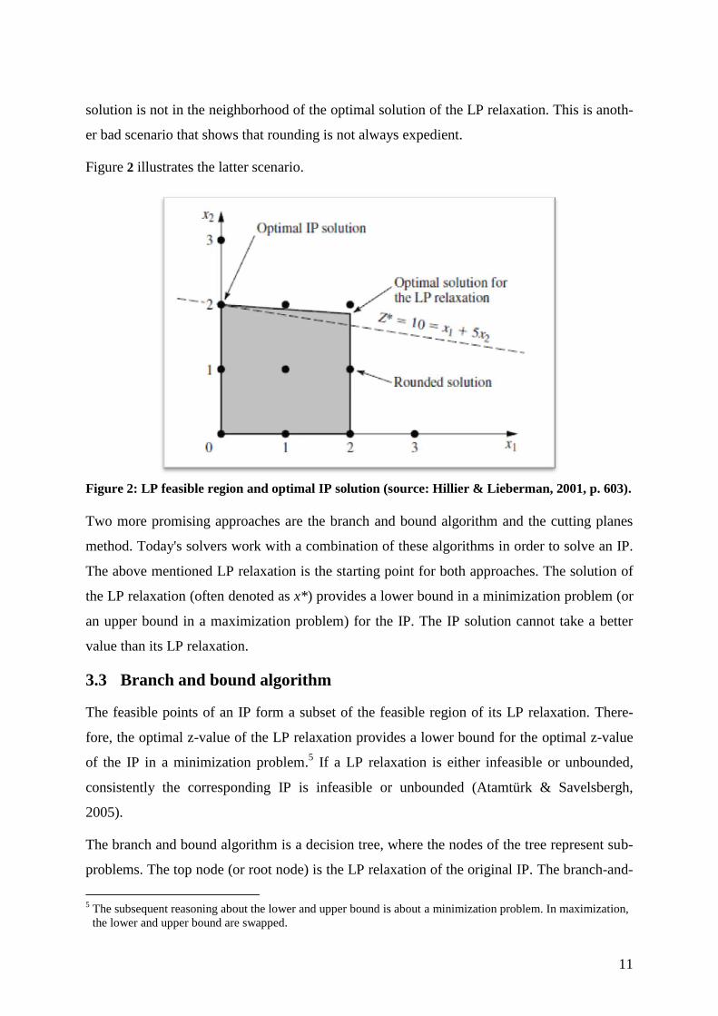
solution is not in the neighborhood of the optimal solution of the LP relaxation. This is anoth-

er bad scenario that shows that rounding is not always expedient.

Figure 2 illustrates the latter scenario.

Figure 2: LP feasible region and optimal IP solution (source: Hillier & Lieberman, 2001, p. 603).

Two more promising approaches are the branch and bound algorithm and the cutting planes

method. Today's solvers work with a combination of these algorithms in order to solve an IP.

The above mentioned LP relaxation is the starting point for both approaches. The solution of

the LP relaxation (often denoted as x*) provides a lower bound in a minimization problem (or

an upper bound in a maximization problem) for the IP. The IP solution cannot take a better

value than its LP relaxation.

3.3 Branch and bound algorithm

The feasible points of an IP form a subset of the feasible region of its LP relaxation. There-

fore, the optimal z-value of the LP relaxation provides a lower bound for the optimal z-value

of the IP in a minimization problem.5 If a LP relaxation is either infeasible or unbounded,

consistently the corresponding IP is infeasible or unbounded (Atamtürk & Savelsbergh,

2005).

The branch and bound algorithm is a decision tree, where the nodes of the tree represent sub-

problems. The top node (or root node) is the LP relaxation of the original IP. The branch-and-

5 The subsequent reasoning about the lower and upper bound is about a minimization problem. In maximization,

the lower and upper bound are swapped.

12

bound algorithm iteratively divides the solution space into subproblems, referred to as chil-

dren nodes. The subproblems have the same complexity as the original IP, but the solution

space is getting smaller. Two children nodes are created by rounding a variable xi with a frac-

tional, non-integer value in the LP relaxation. In order to split the problem, new constraints

are introduced: For the first subproblem variable xi is smaller or equal to the rounded down

integer, while for the second subproblem variable xi is larger or equal to the next rounded up

integer. For instance, if a variable xi takes a value of 3.4 in the LP relaxation, then the LP re-

laxation is divided into two subproblems by adding a new constraint to each subproblem: The

next lower integer value is 3, the next higher is 4. To one subproblem the constraint xi ≤ 3 is

added, to the other xi ≥ 4. In case of binary variables (1 or 0), one can simply introduce the

new constraints in the form xi = 0 and xi = 1, respectively.

The resulting two subproblems are again solved as a LP relaxation. If the solver does not find

an integer solution, the subproblems are further branched, as long as an integer solution is

found.

Figure 3: Branch and bound algorithm (source: Pochet & Wolsey, 2006, p. 87).

Figure 3 is a visualization of the division of the LP relaxation feasible region in subproblems.

The LP relaxation (green area) has its optimum at point a, which is not an integer solution.

The picture shows a branching on variable x1. The LP relaxation of the two subproblems P1

13

and P2 do not deliver integer solutions (points b and c). Hence further branching on variable

x2 is required.

Once the first feasible integer solution is found, its z-value is the first incumbent and an upper

bound of the IP. This is not necessarily the optimal solution. Thus the algorithm further ex-

plores nodes, until an optimal or a near optimal solution is found. For this purpose, the user

defines a stop criterion in the solver's settings.

The branching mechanism has two important decisions at every step: Which fractional varia-

ble is chosen next for further branching and which node is examined first. The effectiveness

of the branch and bound depends strongly on how quickly the upper and lower bound con-

verge (Atamtürk and Savelsbergh, 2005). Therefore, one would like to choose the variable for

branching that limits these bounds as fast as possible. One strategy is to branch the most frac-

tional variable, in other words the variable whose fraction is closest to ½. However, Achter-

berg, Koch and Martin (2005) show that this strategy performs even worse than the random

choice of a branching variable.

More promising, but also more laborious, is the strong branching technique: A branching is

made on a trial basis on every fractional variable. The most promising variable is chosen for

the further branching. Because strong branching implies a lot of calculation, it is not efficient

to perform it at every node.

A third strategy to find the most promising variable for further branching is the pseudo cost

branching: For each fractional variable, an estimate is provided for the decrease of the objec-

tive function value if the variable is rounded down and rounded up (Lodi, 2010). The pseudo

cost is defined as:

and

Parameter represents the pseudo costs at rounding down variable xi, is the change of

the z-value in the objective function by rounding down the variable and fi is the fraction of the

variable (e.g. if the variable xi has a value of 7.3, its corresponding fraction fi is 0.3).

The algorithm chooses the variable with the maximum decrease of the z-value by rounding up

or down.

After having chosen the variable for further branching, the second upcoming decision is the

node selection. There are two different strategies: Choosing the most promising node, which

14

is the node with the smallest upper bound (in a minimization problem). This is known as best

bound or best first search. The second strategy is the depth first or diving search. This is

where all children nodes of a subproblem are examined. One only backtracks if a node is

fathomed and further branching on this node becomes impossible or needless. This occurs if

the problem becomes infeasible or its bound is inferior to the current incumbent. The best first

strategy explores fewer nodes but needs more memory, because there are more active sub-

problems which need to be elicited. In addition, the subproblems have only a weak resem-

blance to each other, which leads to longer calculation. On the other hand, the depth first

search explores more and sometimes useless nodes. But the changes from one subproblem to

the next are small, since only one bound of a variable changes. This allows the solver to cal-

culate the new subproblem in a shorter time.

Most solvers use hybrid techniques, mixing best first and depth first search. At the beginning,

it is most promising to concentrate on depth first search in order to find a good solution quick-

ly. In a later stage of the search, the emphasis is more on the best first search in order to im-

prove the global bound (Atamtürk & Savelsbergh, 2005).

The lower bound (in a minimization problem) is the best possible solution of a current node

and its descendants. The incumbent is the best integer feasible solution found so far. Pruning

a node is the term for eliminating a node. This happens if a node's bounding function is worse

than the actual incumbent or if a node does not contain a feasible solution, namely when a

constraint cannot be satisfied. The branch and bound algorithm stops if the incumbent z-value

is equal to the value of the initial LP relaxation, or if all nodes are pruned, hence the incum-

bent is the best possible solution.

3.4 Cutting planes method

The cutting planes method cuts down the solution space at its periphery, as opposed to branch

and bound that severs the solution space into two halves. The method was first described by

Ralph E. Gomory in 1958 (Gomory, 1958). Additional constraints are added to the LP relaxa-

tion. These constraints are referred to as cutting planes or cuts. They cut away a part of the LP

feasible region without losing any integer feasible points.

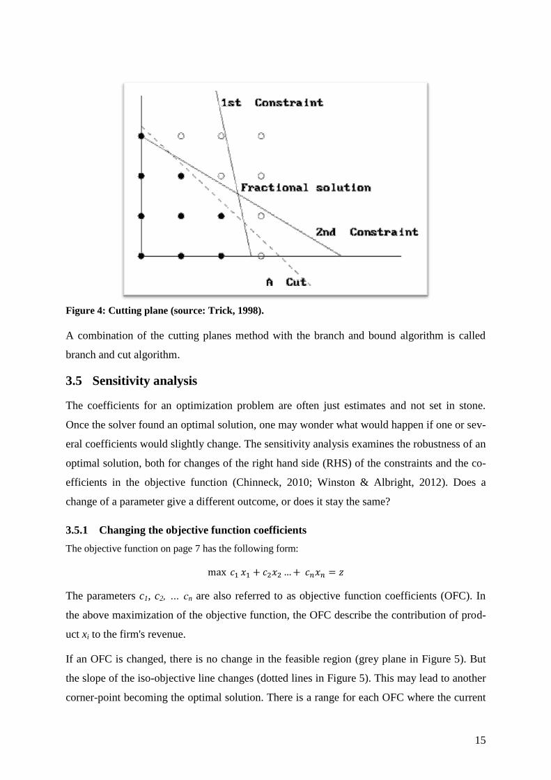
Figure 4 shows a cutting plane (dotted line) that does not cut away any integer solution from

the feasible region. It is even possible to add cuts that remove a part of the MIP feasible re-

gion, as long as the integer optimal solution remains in the solution space.

15

Figure 4: Cutting plane (source: Trick, 1998).

A combination of the cutting planes method with the branch and bound algorithm is called

branch and cut algorithm.

3.5 Sensitivity analysis

The coefficients for an optimization problem are often just estimates and not set in stone.

Once the solver found an optimal solution, one may wonder what would happen if one or sev-

eral coefficients would slightly change. The sensitivity analysis examines the robustness of an

optimal solution, both for changes of the right hand side (RHS) of the constraints and the co-

efficients in the objective function (Chinneck, 2010; Winston & Albright, 2012). Does a

change of a parameter give a different outcome, or does it stay the same?

3.5.1 Changing the objective function coefficients

The objective function on page 7 has the following form:

The parameters c1, c2, … cn are also referred to as objective function coefficients (OFC). In

the above maximization of the objective function, the OFC describe the contribution of prod-

uct xi to the firm's revenue.

If an OFC is changed, there is no change in the feasible region (grey plane in Figure 5). But

the slope of the iso-objective line changes (dotted lines in Figure 5). This may lead to another

corner-point becoming the optimal solution. There is a range for each OFC where the current

16

optimal point stays the best solution. This range is specified with an allowable increase and an

allowable decrease of the coefficient. Nevertheless, the z-value changes, except the corre-

sponding decision variable is zero. For this case a solver's sensitivity report specifies how

much higher the coefficient (in a maximization problem) must be before the corresponding

variable becomes positive, also known as "reduced cost".

Figure 5: Changing an objective function coefficient (source: Bisschop, 2011).

In Figure 5, the optimal point for objective function 1 is point a on the horizontal axis. The

objective function 3 has its optimal corner point b. There are multiple optimal solutions for

objective function 2 all along the line between a and b including both corner points. This is

because the iso-objective line is parallel to the constraint connecting the two points a and b.

3.5.2 Changing the right hand side of a constraint

The RHS of a constraint (b1 in the equation below) represents an upper bound of a scarce re-

source in a production process.

An increase of the RHS in a smaller or equal-constraint means that the constraint is relaxed. The

shadow price of a constraint's RHS quantifies the change in the objective function value by

changing the RHS by one unit. If a constraint is nonbinding, its shadow price is zero.

A change in the RHS of a binding constraint also changes the feasible region of the optimiza-

tion problem. The slope of the constraint line does not change, but its position is higher or

17

lower, as the arrow in Figure 6 indicates. If the moving constraint belongs to the optimal cor-

ner point solution, then this affects also the optimal solution as the dotted lines in Figure 6

show.

Figure 6: Relaxing the right hand side of a constraint (source: Bisschop, 2011).

Figure 7: Illustration of the allowable range for a constraint's RHS (source: Bisschop, 2011).

A sensitivity report also indicates how much the RHS is allowed to change, before another

corner point becomes optimal. Figure 7 illustrates the allowable range of the RHS. The three

parallel lines represent the same constraint with various RHS. In the original problem, corner

point a is the optimal solution. A tightening of the RHS moves the constraint downwards, or

rather to the left. The optimal solution is still the same corner point, but it moves to the left

towards point b. A further moving to the left would also change the optimal corner point,

18

since another constraint is becoming active (or binding): The green constraint gets inactive

and the blue gets active. The same is true for a relaxing of the RHS towards the optimal point

c. If the constraint is moving further to the right, it becomes nonbinding.

3.5.3 Sensitivity analysis in mixed integer programming

The above contemplation does not take into account the integer restrictions of an IP, but is

rather based on LP. IP optimal solutions are usually interior points of its LP relaxation feasi-

ble region. Hence the statements of a sensitivity analysis must be interpreted with caution.

Sensitivity analysis for IP is still at an early stage. Existing concepts make use of the duality

theory (e.g. Wolsey, 1981 and Guzelsoy & Ralphs, 2011). There is no implementation of sen-

sitivity analysis for IP in solvers, which is also true for the standard solver for Excel.

Hence the sensitivity analysis executed in section 6.4 is rather of qualitative than quantitative

nature: In a first step, modifiable variables are detected. Afterwards, its values are changed

manually and the impact on the problem is evaluated. OpenSolver provides a Quick Solve

feature which should accelerate this hand-knitted analysis. According to Mason (2012), they

are able to reduce the run time for their scheduling problem from one hour to one minute.

Unfortunately, Quick Solve does not accelerate the calculation time in the present MIP, the

reason for this phenomenon is unknown.

19

4 The scheduling model

4.1 Introduction to the scheduling model

Ferrand et al. (2011) developed a schedule for the five physicians of a recently opened emer-

gency department at the Cincinnati Children's Hospital Medical Center by formulating a MIP.

In cooperation with the physicians, they defined a set of compulsory and flexible rules for the

schedule.

4.1.1 Compulsory rules

A particular schedule is only feasible if all compulsory rules are met: The total number of

shifts assigned to each physician is fixed. The proportion for each type of shifts is as close as

possible to one-third. At least 20% of the AM shifts must be assigned on Friday. The total

number of shifts worked on a Friday and weekends is fixed.

The physicians have their preferences: Weekend shifts should be batched together. They nev-

er work more than two weekends in a row. At most four shifts are assigned in any given

week. There are no single workdays; at least two workdays are batched together. If the last

worked day is an overnight shift, the physician has at least two days off. If the last shift

worked is a PM shift, the break should be at least one day off followed by either a PM or

overnight shift, or two days if the next assigned shift is an AM shift. If the last worked day is

an AM shift, then the break can be only one day.

4.1.2 Flexible rules

There are three flexible rules which are nice to have, but must not be fulfilled, in contrast to

the compulsory rules. If a flexible rule is violated, a penalty kicks in in the objective function.

The goal of the optimization is to minimize these penalties due to violations of the soft con-

straints. Unlike the standard form of an objective function presented in chapter 3.1, the objec-

tive function does not have the form of a sum-product ( ), but is rather a weighted sum of

deviations.

The three flexible rules are the following:

1. Only one physician is assigned to work a shift.

2. If a weekend is off, then also the previous Friday or the following Monday should be

off.

20

3. Not more than two consecutive overnight shifts should be assigned in a Monday to

Thursday time slot.

One physician works only overnight, hence the last rule does not apply to him.

4.2 Model formulation

In this section the model is presented as in the original formulation of Ferrand et al. (2011).

Section 4.3 reflects on how the model can be simplified, both for a better comprehensibility

and an easier implementation in Excel or GAMS. Contrary to the reasoning in the paper of

Ferrand et al. (2011), the simplified is not significantly slower (see section 6.7).

4.2.1 Sets

I 1,2,3 set of shifts, 1 ≡ AM, 2 ≡ PM, 3 ≡ overnight shift

J 1,…, 56 set of days within the eight-week cycle

K 1,…, 5 set of physicians in the team

L 1,…, 8 set of weeks within the eight-week cycle

4.2.2 Variables

The decision variables define each physician's work schedule. There is one variable for

each shift at each day and each physician, altogether 840 binary variables (3 shifts times 56

days times 5 physicians).

1 if physician k works shift i on day j, 0 otherwise

A second group of variables measures the deviation from three flexible rules introduced

above. The deviation variables are nonnegative and continuous variables. Elsewise the solver

would tend to give these variables a negative value, since the objective function is a weighted

sum of the deviation variables and its z-value is minimized. This would provoke an unwished

deviation from the desired goals and lead to a negative and meaningless z-value in the objec-

tive function.

It is not necessary and even counterproductive to define these deviation-variables (or d-

variables) as binary variables, even though they all take a value of 1 or 0. All d-variables are

defined in combination with the binary x-variables. They automatically adopt a binary value.

Nonetheless it is helpful to define the d-variables as continuous variables: The fewer binary variables

in a model, the faster the calculation is.

21

deviation from the goal of ensuring that only one physician is assigned to work shift i

on day j

deviations from the goal that if weekend l is off, also the adjacent Friday or Monday

is a day off for physician k

deviation from the goal of physician k working two or fewer overnights in a row from

Monday to Thursday

There are 168 variables, 40

variables and between 32 and 96 variables, depending

on the exact problem definition (see section 0 0).

Finally, there is a group of auxiliary variables (or s-variables) concerning the successive

working days and days off. These variables are continuous. As before the d-variables, also the

s-variables are defined in combination with the binary x-variables and only take binary val-

ues.

1 if physician k does not work on day (j-1) but works on day j, 0 otherwise

1 if physician k works on day (j-1) but not on day j, 0 otherwise

1 if physician k does not work on Saturday j, 0 otherwise, for j = 6,13,…,55

1 if physician k does not work on Sunday j, 0 otherwise, for j = 7,14,…,56

1 if physician k does not work overnight on day j, 0 otherwise

There are 280 and as many

variables, 40 and

variables and 128 variables.

To sum up, only the -variables are defined as binary variables, although all variables take a bina-

ry value. The model in its original design contains 840 binary, 304 positive and 768 continuous varia-

bles thus a total of 1,912 variables.

The model can be formulated in a way that all s-variables can be omitted. In the modified ver-

sion, the number of variables is reduced to 840 binary, 240 positive and 0 continuous variables thus a

total of 1080 variables!

22

4.2.3 Objective function

The objective function aims to minimize the deviation from the soft constraints. There is more

weight on the deviation of the goal that only one physician is assigned per shift ( ), which is

the prioritized goal.

∑∑

∑∑

∑∑

4.2.4 Constraints

a) Constraints regarding breaks between two shifts

If physician k works in the afternoon on day j, then he does not work in the morning on either

day (j+1) or (j+2).

In other words, if is 1 (this variable represents the afternoon shift of physician k at day j),

then ( ) and ( ) (thus the AM shift the next and the next but one day of physician k

at day j) have to be 0 in order to meet equations (2) and (3). If is 0, the other variables

can either be 0 or 1.

Equations (2) to (7) apply for ∀ j, k.

( ) (2)

( ) (3)

If physician k works overnight on day j, then he does not work the AM and PM shift of the

next two days (j+1) and (j+2).

( ) (4)

( ) (5)

( ) (6)

( ) (7)

b) Constraints on the demand

There are two physicians assigned per shift at most, or even better only one physician. If there

are two physicians assigned to the same shift, then one of them should be physician 3 or 5,

since these two physicians are required to work a fraction of their workload at another hospi-

tal department.

23

Equations (8) and (9) apply for ∀ i, j.

∑

(8a)

(8b)

(9)

Equation (8a) defines the deviation variable : In case two physicians are assigned for one

shift, is 1. If there is no or only one physician assigned for a shift,

is 0. Equation (8b)

assures that at most two physicians are assigned. If there were three, equation (8a) would be

violated. Eventually, equation (9) guarantees that if two physicians are assigned (accordingly

is one), at least one of both variables and is also one.

c) Constraint on the supply

The physicians work a certain amount of shifts per eight-week cycle. Parameter represents

the workload of physician k per cycle. This parameter is exogenously given (see Table 1 be-

low).

∑∑

∀ (10)

d) Constraints regarding a fair distribution of shifts

The proportion of AM, PM and overnight shifts for each physician is limited as close as pos-

sible to one third for each type of shifts. This constraint does not apply for physician 1, be-

cause he only works overnight.

∑

∀ (11)

Parameter aik is the lower and bik the upper bound on the number of shifts of type i for physi-

cian k per cycle. These parameters should be as close as possible to one third of the workload

. Also the fractions are also exogenously given:

24

k Lk aik bik

1 24 - -

2 24 8 8

3 19 6 7

4 26 8 9

5 26 8 9

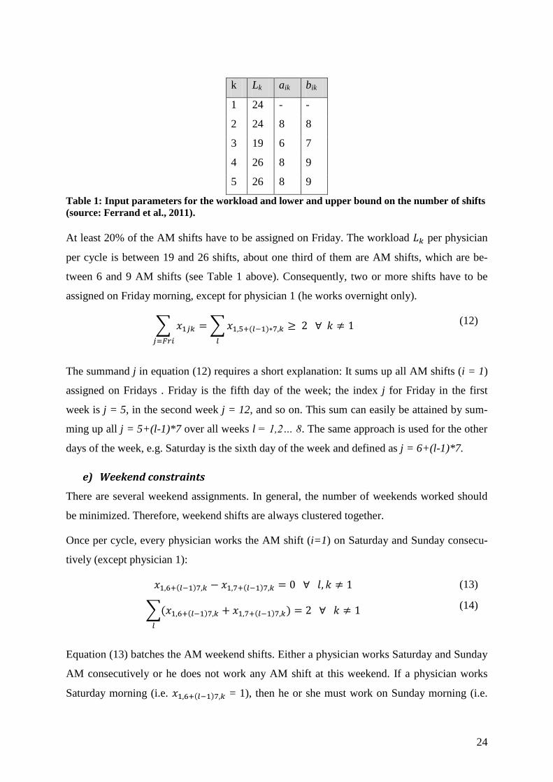
Table 1: Input parameters for the workload and lower and upper bound on the number of shifts

(source: Ferrand et al., 2011).

At least 20% of the AM shifts have to be assigned on Friday. The workload per physician

per cycle is between 19 and 26 shifts, about one third of them are AM shifts, which are be-

tween 6 and 9 AM shifts (see Table 1 above). Consequently, two or more shifts have to be

assigned on Friday morning, except for physician 1 (he works overnight only).

∑

∑ ( )

∀ (12)

The summand j in equation (12) requires a short explanation: It sums up all AM shifts (i = 1)

assigned on Fridays . Friday is the fifth day of the week; the index j for Friday in the first

week is j = 5, in the second week j = 12, and so on. This sum can easily be attained by sum-

ming up all j = 5+(l-1)*7 over all weeks l = 1,2… 8. The same approach is used for the other

days of the week, e.g. Saturday is the sixth day of the week and defined as j = 6+(l-1)*7.

e) Weekend constraints

There are several weekend assignments. In general, the number of weekends worked should

be minimized. Therefore, weekend shifts are always clustered together.

Once per cycle, every physician works the AM shift (i=1) on Saturday and Sunday consecu-

tively (except physician 1):

( ) ( ) ∀ (13)

∑( ( ) ( ) )

∀ (14)

Equation (13) batches the AM weekend shifts. Either a physician works Saturday and Sunday

AM consecutively or he does not work any AM shift at this weekend. If a physician works

Saturday morning (i.e. ( ) = 1), then he or she must work on Sunday morning (i.e.

25

( ) = 1) in order to fulfill equation (13). The physicians work AM shifts at exactly

one weekend per cycle; which is induced by equation (14).

Once per cycle, physicians 2, 3 and 5 work the PM shift (i=2) Friday, Saturday and Sunday

consecutively:

( ) ( ) ∀ (15)

( ) ( ) ∀ (16)

∑( ( ) ( ) ( ) )

(17)

Equations (15) and (16) batch the PM shifts from Friday, Saturday and Sunday, while equa-

tion (17) effectuates that PM shifts are scheduled at exactly one weekend.

Physician 4 is required to work three Fridays PM or overnight shifts per cycle. Therefore, two

Friday PM shifts and one Friday overnight shift are assigned on in equations (20) and (21).

Equation (18) allows in combination with equation (19) that physician 4 works Friday PM but

not Saturday PM at the same weekend. To sum up, physician 4 works one weekend PM shifts

consecutively, another weekend overnight shifts consecutively (besides, this is redundant with

equations (23) to (25)) and an additional PM shift on a Friday with the following weekend

off. This explains the RHS value of 7 (4 PM + 3 overnight shifts) in equation (22), which

sums up all PM and overnight shifts (i=2,3) from Friday to Sunday over the eight week cycle.

( ) ( ) ∀ (18)

( ) ( ) ∀ (19)

∑ ( )

(20)

∑ ( )

(21)

∑∑( ( ) ( ) ( ) )

(22)

26

Physicians 2 to 5 once work Friday, Saturday and Sunday overnight consecutively, physician

1 three times:

( ) ( ) ∀ (23)

( ) ( ) ∀ (24)

∑( ( ) ( ) ( ) )

{ ∀

(25)

Equations (23) and (24) batch the weekend overnight shifts. Equation (25) causes one week-

end with overnight shifts for physicians 2 to 5 and three weekends with overnight shifts for

physician 1.

No physician works more than two weekends (Saturday and Sunday) in a row. The sum of all

weekend shifts per physician at three consecutive weekends is less or equal to 4:

∑∑ ( )

( ) ∀ [ ] (26)

f) Constraints concerning weekly workload and succession of shifts

The physicians work at most four shifts in any given week:

∑∑ ( )

∀ (27)

There is a maximum of three consecutive working days, except for physician 1, who works at

most four consecutive days (see equation (45)).

∑∑

∀ [ ] (28)

The next four sets of constraints can be achieved with a simpler formulation with fewer ine-

qualities by avoiding auxiliary variables. Ferrand et al. (2011) claims that the solver performs

better with the auxiliary variables, because each constraint comprises fewer binary variables.

According to the authors, this is especially important if the model is expanded to a longer cy-

cle or to more physicians. Despite these concerns in Ferrand et al. (2011), a simpler model

27

formulation by avoiding the s-variables is proposed in section 0. For a critical acclaim of this

issue see section 6.7.

The working days are batched to at least two consecutive days (except for physician 1 who

works at least three consecutive days, see equations (46) to (50)). Equations (29) to (31) de-

fine the variable . Equation (32) ensures that if a physician is not working on day (j-1) but

on day j, then he must work also on day (j+1). Equations (29) to (32) apply for ∀ .

∑

(29)

∑ ( )

(30)

∑

∑ ( )

(31)

∑ ( )

(32)

∑ ( ) ∑

conflicting

equations

1 1 1 30

1 0 1 -

1 0 0 29

1 1 0 29, 30

0 1 1 -

0 0 1 31

0 1 0 -

0 0 0 -

Table 2: Variable analysis for equations (29) to (31).

Table 2 above shows that is 1 if and only if a physician is working on day j but not work-

ing on day (j-1). In all other cases, is 0. If

is 1, then a physician has to be assigned for a

shift on day (j+1), which is ensured with equation (32).

Between groups of overnight shifts, the physicians have at least two days off. Equations (33)

to (35) define , and equation (36) ensures that if a physician is working overnight on day (j-

1) but not on day j, then he cannot be assigned to work overnight on day (j+1). Equations (33)

to (36) apply for ∀ .

28

( ) (33)

(34)

( ) (35)

( ) (36)

( )

conflicting

equations

1 1 1 34

1 0 1 33, 34

1 0 0 33

1 1 0 -

0 1 1 -

0 0 1 -

0 1 0 35

0 0 0 -

Table 3: Variable analysis for equations (33) to (36).

Variable is 1, if and only if a physician is working overnight on day (j-1), but not working

overnight on day j. If so, the physician cannot be assigned for an overnight shift on day (j+1),

as defined in equation (36). In all other cases is 0.

Equation (36) only considers the overnight shift of day (j+1). There is no statement about the

AM and PM shift. This is not necessary because it is impossible to assign an AM or PM shift

on day (j+1) due to equations (6) and (7).

The next two groups of constraints are about the soft rules. If these constraints are not ful-

filled, a penalty comes into play.

If the physician has a weekend off, also the adjacent Friday or Monday is a day off. Equations

(37) to (39) define and

. Equation (40) ensures that if a physician has a weekend off,

then either Monday or Friday is off too; otherwise, a penalty comes into play. Equations (37)

to (40) apply for ∀ .

( ) ∑ ( )

(37)

( ) ∑ ( )

(38)

29

( ) ( )

∑ ( )

∑ ( )

(39)6

( ) ( )

∑ ∑

( )

(40)

If a physician works on Saturday, then has to be 0 due to equation (37). The same is true

for Sunday shifts and in equation (38). Weekend shifts are always batched (due to equa-

tions (13), (16), (19) and (24)); in other words both sums ∑ ( ) and ∑ ( )

are either 0 or 1. If a weekend is off (which is equivalent to both sums are 0), and

are

both 1 in order to fulfill equation (39). As a consequence, only the following two combina-

tions are possible:

∑ ( ) ∑ ( )

1 1 0 0

0 0 1 1

Table 4: Variable analysis for equations (37) to (39).

The following table shows all possible combinations with regard to equation (40). Only if the

weekend (Saturday and Sunday) is off and the physician works at both Friday and Monday,

the penalty kicks in.

∑ ∑ ∑ ∑

1 1 1 0 0 1 1

1 1 1 0 0 0 0

1 1 0 0 0 1 0

1 1 0 0 0 0 0

0 0 0 or 1 1 1 0 or 1 0

Table 5: Variable analysis for equation (40).

For physicians 2 to 5, it would be more intelligible to formulate equation (40) as follows:

( ) ( )

∑ ∑

( )

But this formulation is invalid for physician 1: Because he works up to four consecutive

shifts, it is also possible that he works from Friday to Monday in a row. The above formula-

tion would charge a penalty in that case, which is incorrect. In order to eliminate this error,

both s-variables are multiplied by 2 and the RHS is adjusted to 5.

6 This equation could be formulated more precisely with equality instead of larger or equal.

30

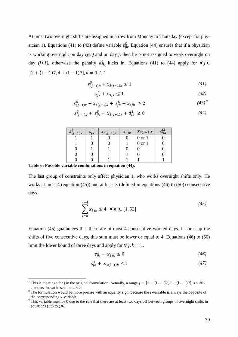
At most two overnight shifts are assigned in a row from Monday to Thursday (except for phy-

sician 1). Equations (41) to (43) define variable . Equation (44) ensures that if a physician

is working overnight on day (j-1) and on day j, then he is not assigned to work overnight on

day (j+1), otherwise the penalty kicks in. Equations (41) to (44) apply for ∀

[ ( ) ( ) ] . 7

( ) ( ) (41)

(42)

( ) ( )

(43) 8

( )

( ) (44)

( )

( ) ( )

1 1 0 0 0 or 1 0

1 0 0 1 0 or 1 0

0 1 1 0 09 0

0 0 1 1 0 0

0 0 1 1 1 1

Table 6: Possible variable combinations in equation (44).

The last group of constraints only affect physician 1, who works overnight shifts only. He

works at most 4 (equation (45)) and at least 3 (defined in equations (46) to (50)) consecutive

days.

∑

∀ [ ] (45)

Equation (45) guarantees that there are at most 4 consecutive worked days. It sums up the

shifts of five consecutive days, this sum must be lower or equal to 4. Equations (46) to (50)

limit the lower bound of three days and apply for ∀ .

(46)

( ) (47)

7 This is the range for j in the original formulation. Actually, a range [ ( ) ( ) ] is suffi-

cient, as shown in section 4.3.2. 8 The formulation would be more precise with an equality sign, because the s-variable is always the opposite of

the corresponding x-variable. 9 This variable must be 0 due to the rule that there are at least two days off between groups of overnight shifts in

equations (33) to (36).

31

( ) (48)

( ) (49)

( ) (50)

Equations (46) to (49) are similar to equations (29) to (32), except that physician 1 works

overnight shifts only. Equation (50) intends that at least three consecutive worked days are

batched. Variable is one, if physician 1 works on day j, but not on day (j-1). In this situa-

tion, he must work on days (j+1) - this is achieved in equation (49) - and also on day (j+2) in

order to fulfill equation (50).

4.3 Reformulations

During the implementation of the original model, it became evident that some equations can

be fused together, dropped or formulated in a simpler way. Other equations are missing in the

original formulation. Thanks to the reformulation effort, the number of constraints is reduced

from 5,777 in the original formulation to 3,336 in the modified formulation.

4.3.1 Fusing equations

Equations (4) and (5) as well as (6) and (7) can be fused together: If a physician works over-

night, he cannot be assigned for both the AM and PM shift of the next two days, so these var-

iables are all 0. Even if there is no overnight shift, a physician works at most one shift the

following day. Hence the sum of the variables for the AM and PM shift the next day does not

exceed 1.

( ) ( ) (4r)10

( ) ( ) (6r)

Also equations (15) and (16) can be fused together by summing up both equations. Table 7

below shows that also the new equation batches the PM weekend shifts (Friday to Sunday).

( ) ( ) ( ) ∀ (15r)

10

The r stands for reformulated.

32

LHS11

feasible

1 1 1 0 yes

0 0 0 0 yes

1 0 0 2 no

0 1 0 -1 no

0 0 1 -1 no

1 1 0 1 no

1 0 1 1 no

0 1 1 -2 no

Table 7: Variable analysis and corresponding LHS for equation (15r).

Equations (21) and (22) about the weekend assignments for physician 4 are rather confusing,

since they unnecessarily mix PM and overnight shifts. It is easier to consider these two types

of shifts independently, because equations (23) to (25) exclusively deal with the overnight

shifts at weekends for all physicians. Equation (21) is redundant to equations (23) and (25)

and can be left out. Equation (22) is reformulated ignoring the overnight shifts of physician 4.

The RHS is 4 because physician 4 works once Friday to Sunday PM shifts consecutively plus

an additional Friday PM shift followed by a weekend off.

∑( ( ) ( ) ( ) )

(22r)

Equations (23) and (24) can be merged together, as equations (15) and (16).

( ) ( ) ( ) ∀ (23r)

4.3.2 Reformulation of equations (29) to (44) and (46) to (50) by avoiding the auxiliary

variables

These 20 equations representing 2,840 constraints can be replaced by only five new equa-

tions, resulting in 688 constraints. The reformulation avoids 2,152 constraints and all 768

s-variables!12

The authors justify their formulation with a tighter problem formulation for the

branch and bound algorithm. Their reasoning: Every equation only includes few variables,

which accelerates the calculation time. Fewer variables per equation imply less recalculation

of each equation in the branch and bound algorithm. But the quantity of equations and varia-

bles, although discrete, is much higher, which results in more calculation. The authors believe

11

LHS stands for left-hand side. 12

A listing of these numbers is done in the appendix.

33

that their tighter equation formulation outweighs the enhanced number of equations, especial-

ly for a larger problem with more than five physicians.13

a) Equations (29) to (32): Physician k works at least two consecutive days

The four equations can be replaced by the equation (29r):

∑( ( ) ( ) )

∀ (29r)

case ∑ ( ) ∑ ∑ ( ) ∑ ( ) ∑ ( ) LHS

i 1 1 1 1

ii 0 0 0 0

iii 1 1 0 0 1

iv 0 1 0 - 1

v 0 0 1 1 1

vi 1 1 0 0

vii 1 1 0 1 1 2

viii 0 1 1 0

Table 8: Variable analysis and resulting LHS for equation (29r).

The table above shows all possible combinations. Basically, only case iv) is not allowed, be-

cause a working day is surrounded by two days off. There is also a single workday in case iii).

This is only allowed if the physician works also on day (j-1). Otherwise, the above constraint

is not fulfilled for day (j-1). The same is true for case v), which is only feasible if the physi-

cian is working on day (j+3), and case vii), where the physician has to work on either day (j-

1) and (j+3).

b) Equations (33) to (36): Give at least two days off between groups of overnight

shifts

Since an overnight shift is never followed by an AM or PM shift at the next and the next but

one day (this is ensured by equations (4) to (7)), equation (33r) only comprises the overnight

shifts.

( ) ( ) ∀ (33r)

13

See e-mail correspondence with Yann Ferrand in the appendix.

34

( ) ( ) LHS

i 1 1 1 1

ii 0 0 0 0

iii 1 0 0 1

iv 0 1 0 - 1

v 0 0 1 1

vi 1 1 0 0

vii 1 0 1 2

viii 0 1 1 0

Table 9: Variable analysis and resulting LHS for equation (33r).

The only infeasible combination is case vii), because there is only one day off between two

overnight shifts. Note that combinations iv), vi) and viii) are basically feasible in this narrow

observation, but no overnight shift on day (j-1) and/or (j+3) is allowed.

c) Equations (37) to (40): If a weekend is off, then also the previous Friday or

the following Monday is off

∑( )

∀

(37r)

Or, the same formulation with index l:

∑( ( ) ( ) ( ) ( ) )

∀

(37r)

If Saturday and Sunday are off and the adjacent Friday and Monday are both working days, a

penalty kicks in.

∑ ∑ ∑ ∑ LHS

i 1 0 0 1 1 1

ii 1 0 0 0 0 1

iii 0 0 0 1 0 1

iv 0 0 0 0 0 0

v14

1 1 1 1 0 0

vi 1 1 1 0 0 - 1

vii 0 1 1 1 0 - 1

viii 0 1 1 0 0 - 2

Table 10: Variable analysis and LHS for equation (37r).

14

Only physician 1 is allowed to work four consecutive days (equation (45)).

35

d) Equations (41) to (44): Assign at most two overnight shifts in a row from

Monday to Thursday

( ) ( )

∀ [ ( ) ( ) ]

(41r)

This reformulation uses a narrower range for j than the original formulation. It is assumed that

a succession of overnight shifts on Wednesday, Thursday and Friday does not cause a penalty.

A more detailed consideration demonstrates that this succession is not even possible at all!

Equations (23) to (25) batch Friday overnight shifts with weekend overnight shifts. If a physi-

cian works Friday night, he works also Saturday and Sunday night, which are three consecu-

tive workdays. Since the physicians work at most three consecutive days, it is impossible that

a physician works Thursday and Friday night consecutively. Therefore, it is sufficient to

check only for the time slot from Monday to Thursday. If there are three consecutive over-

night shifts from Monday to Thursday, the penalty kicks in.

Physicians 2 to 5 work at most three shifts in a row. If the last shift is an overnight shift, there

are at least two days off, as defined in equations (33) to (36) or (33r) respectively. With this

fact in mind, it is even sufficient to check if there are more than two overnight shifts assigned

in a Monday to Thursday time slot. If so, the penalty kicks in. As a consequence, only a

single constraint remains per week and physician:

∑

∀ ( )

(41rr)

e) Equations (46) to (50): Physician 1 works at least three consecutive days

This issue can be achieved in two steps: In the first step equation (29r) becomes also valid for

physician 1, which ensures that at least two consecutive days are grouped.

∑( ( ) ( ) )

∀ (29r)

After ensuring that physician 1 is assigned to at least two consecutive days, a third or fourth

workday is attached due to equation (46r).

36

∑( ( ) ( ) ( ) )

∀ (46r)

The following table does not list all combinations, but only combinations that fulfill equation

(29r).

∑ ∑ ( ) ∑ ( ) ∑ ( ) LHS

i 1 1 1 1 0

ii 1 1 1 0 1

iii 0 1 1 1 1

iv 1 0 0 0 - 1

v 1 1 0 0 0

vi 0 1 1 0 2

vii 0 0 1 1 0

viii 0 0 0 1 - 1

Table 11: Variable Analysis and resulting LHS for equation (46r).

Cases i) to iii) conform to both equations and to the rule that physician 1 works at least 3 con-

secutive days. Case vi) does not satisfy equation (46r), because only two worked days are

batched. The other cases fulfill equation (46r), but need an expanded consideration of the

neighboring days (j-2), (j-1), (j+4) and (j+5).

4.3.3 Missing constraints in the original model

There are three issues missing in the original problem formulation.

f) Physician 1 only works overnight

There is no constraint that physician 1 only works overnight. Therefore, an additional con-

straint is proposed:

∀ (51)

Equation (51) is mandatory for a correct solution, otherwise physician 1 is also assigned for

AM and PM shifts.

g) The cyclic nature of the schedule

All calculations in this thesis control if all constraints remain valid over the end of one cycle

to the beginning of the next cycle. This issue is not considered in the above formulations. In

order to do so, the sets for days and weeks are extended to 70 days and 10 weeks. This repre-

sents the first two weeks of the subsequent cycle. In addition, a new constraint is added:

37

( ) ∀ (52)

Thanks to equation (52), all variables of the subsequent cycle (j=56, …, 70) are recur-

rent. Some equations need to be slightly adapted.

The adaption is demonstrated for equation (26): The physicians never work more than two

weekends in a row, which is ensured by equation (26):

∑∑ ( )

( ) ∀ [ ] (26)

In order to control for the cyclic nature of the schedule, equation (26) must apply for

∀ [ ]

Without this adaption, it would be allowed to work in the last week of the cycle and the first

two weeks of the subsequent cycle.

Furthermore, many equations include variables of the following days, e.g. ( ) . For j = 56,

these equations only provide meaningful results if they interact with the variables of the sub-

sequent cycle.15

h) A physician works not more than one shift per day

It is not allowed to work two shifts consecutively and more than one shift per day, but there is

no such constraint in the model. Therefore, equation (53) is proposed:

∑

∀ (53)

Even if this constraint is missing, it is implicitly integrated in the system of constraints, albeit

hidden: In the original formulation, equation (30) assures that only one shift is assigned on

day (j-1) for each physician:

∑ ( )

∀ (30)

15

In the Excel spreadsheet, the equations interacting with the subsequent cycle are highlighted in yellow.

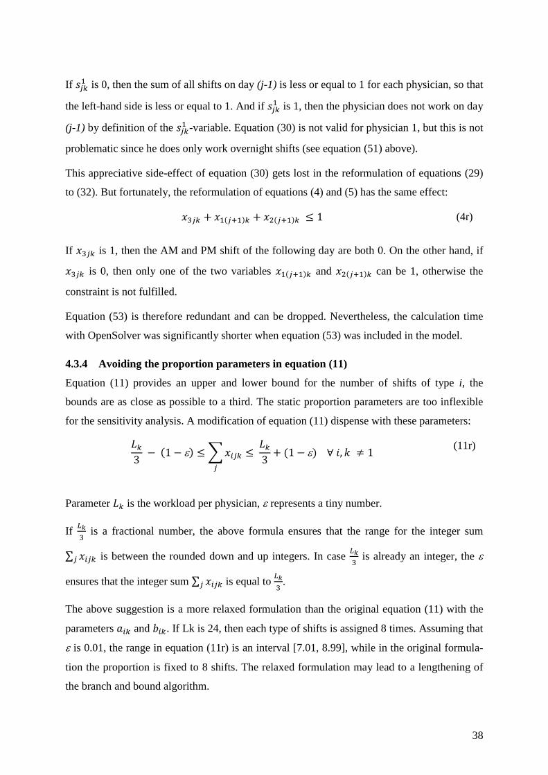
38

If is 0, then the sum of all shifts on day (j-1) is less or equal to 1 for each physician, so that

the left-hand side is less or equal to 1. And if is 1, then the physician does not work on day

(j-1) by definition of the -variable. Equation (30) is not valid for physician 1, but this is not

problematic since he does only work overnight shifts (see equation (51) above).

This appreciative side-effect of equation (30) gets lost in the reformulation of equations (29)

to (32). But fortunately, the reformulation of equations (4) and (5) has the same effect:

( ) ( ) (4r)

If is 1, then the AM and PM shift of the following day are both 0. On the other hand, if

is 0, then only one of the two variables ( ) and ( ) can be 1, otherwise the

constraint is not fulfilled.

Equation (53) is therefore redundant and can be dropped. Nevertheless, the calculation time

with OpenSolver was significantly shorter when equation (53) was included in the model.

4.3.4 Avoiding the proportion parameters in equation (11)

Equation (11) provides an upper and lower bound for the number of shifts of type i, the

bounds are as close as possible to a third. The static proportion parameters are too inflexible

for the sensitivity analysis. A modification of equation (11) dispense with these parameters:

( ) ∑

( ) ∀

(11r)

Parameter is the workload per physician, represents a tiny number.

If

is a fractional number, the above formula ensures that the range for the integer sum

∑ is between the rounded down and up integers. In case

is already an integer, the

ensures that the integer sum ∑ is equal to

.

The above suggestion is a more relaxed formulation than the original equation (11) with the

parameters and . If Lk is 24, then each type of shifts is assigned 8 times. Assuming that

is 0.01, the range in equation (11r) is an interval [7.01, 8.99], while in the original formula-

tion the proportion is fixed to 8 shifts. The relaxed formulation may lead to a lengthening of

the branch and bound algorithm.

39

4.4 Model expansion for up to eight physicians

Ferrand et al. (2011) want to expand the model by adding up to three physicians in order to

run the emergency department independently from external physicians. In this thesis, a first

successful attempt is made: Section 6.5 demonstrates optimal solutions for a simplified

scheduling model with six, seven and eight physicians.

It is not known what individual agreements the new physicians wish to have or if the existing

agreements endure. Instead of assuming any imaginative agreements for the newly added

physicians, the scheduling model is fundamentally simplified and standardized for all physi-

cians.

The present scheduling model is a cyclic schedule without rotation. It allows individual

agreements for each physician. If there are no individual agreements in a standardized model,

a cyclic schedule with rotation would be the best approach to solve the problem. Nevertheless,

the expanded model is formulated as a cyclic schedule without rotation. This allows the

schedule planner to insert individual agreements in the model.

The standardized model contains the following constraints: Each physician is working 24

shifts during the eight week cycle and is assigned to all types of shifts (in particular also phy-

sician 1 works AM and PM shifts). All constraints about individual agreements are dropped.

The weekend shifts remain batched and every physician works exactly three weekends, one

weekend for each type of shifts. All other constraints remain unaltered.

The following table gives an overview of the standardized model's constraints:

Issue Equation No.

After a PM shift, there are no AM shifts assigned the next two days. (2), (3)

After an overnight shift, a physician does not work AM and PM the next

two days.

(4r), (6r)

There are at most two physicians assigned per shift. If more than one phy-

sician is assigned, a penalty kicks in.

(8a), (8b)

40

Every physician works 24 shifts per cycle.

∀

(10e)16

The physicians work exactly eight shifts of each type.

( ) ∀

(11e)

Every physician works three weekends (Saturday and Sunday) per cycle,

one weekend for each type of shifts.

( ) ( ) ∀ (13e)

∑( ( ) ( ) )

∀ (14e)

They never work more than two weekends in a row. (26)

They work at most four shifts per week. (27)

Assign at most three consecutive working days… (28)

… and at least two consecutive days. (29r)

There are at least two days off between groups of overnight shifts. (33r)

If a weekend is off, also the adjacent Friday or Monday is of, otherwise a

penalty kicks in.

(37r)

They do not work more than two overnight shifts in a Monday to Thursday

time window, otherwise a penalty is charged.

(41rr)

They work at most one shift per day. (52)

At least one physician is assigned per each shift (only in the model with

eight physicians).

∑

∀

(54e)

Table 12: Simplified model for the expansion for up to eight physicians (source: own research).

Equation (54e) only applies for the model with eight physicians. It ensures that for every shift

at least one physician is assigned, which is a condition for autonomy. The solver covers every

16

Equations accompanied by an e (for expansion) are introduced for the expanded model. Equations with an r

are the reformulated equations from section 0.

41

shift anyway, even if equation (54e) is dropped. A deserted shift would lead to a double occu-

pancy for another shift, causing an unnecessary deviation.

4.5 Symmetry

Symmetry occurs, if variables are permuted without changing the structure of an IP (Margot,

2010). Symmetry causes additional calculation tasks in the branch and bound algorithm, since

there are several identical solutions. Because of the cyclic nature of the present schedule, the

beginning of a cycle could be in any week. To avoid this aspect of symmetry, a succession of

workdays which occurs only once per cycle can be fixed in the first week. For instance, there

is the exactly one weekend where physician 2 works Friday to Sunday PM shifts consecutive-

ly. Fixing this weekend in the first week is preventing the solver of seven symmetric solu-

tions. The schedule for all physicians is generated around this fixed weekend. There is much

more symmetry in the scheduling model occurring, but according to Margot (2010) it is diffi-

cult to identify symmetry and, as a consequence, making predictions how many symmetrical

solutions exist.

There are other strategies than fixing variables in order to avoid symmetry: Margot (2010)

supposes, amongst others, additional strategies:

- A perturbation in the objective function, for example by adding a small random per-

turbation to the objective function coefficients.

- Adding symmetry breaking inequalities, which remove equivalent subproblems in the

branch and bound algorithm.

The perturbation strategy is helpful for the scheduling model: The deviation variables and

in the objective function do have the same weight. As a consequence, a solution with one

penalty is ceteris paribus equivalent to a solution with one

penalty. In order to avoid

this type of symmetry, the deviation variables in the objective function are all valued with a

different weight:

∑∑

∑∑

∑∑

Now, a -deviation is preferred to a

-deviation, since the penalty of the latter weights

higher.

42

5 Tools used to solve the scheduling problem

The scheduling model was implemented with two different tools, one is an Excel spreadsheet

in combination with the OpenSolver, on the other is a GAMS code in combination with

NEOS Server.

5.1 Excel and OpenSolver

The scheduling model with its approximately 1,900 variables and 5,700 constraints in its orig-

inal formulation is set up in an ordinary Excel file. A cell is reserved for every variable. The

left hand side of every constraint is calculated in a separate cell. Consequently, the spread-

sheet with the original problem formulation includes 1,900 cells for the variables and approx-

imately 4,700 formulas representing the major part of the constraints. Not every constraint

requires a formula, since some constraints only compare different values. Equation (8b) for

example ensures that the -variables are lower or equal to 1.

The standard solver in Excel is restricted to 200 variables and constraints. It is therefore un-

employable for this large-scale problem. OpenSolver overcomes this barrier and has no size

limitations. OpenSolver uses the CBC Solver,17

which is another open-source project of the

Operations Research community.

5.2 GAMS and NEOS Server

GAMS is an algebraic modeling language (General algebraic modeling system) and available

as a free demo version.18

The demo version has its limitation at 300 variables and constraints,

which is not sufficient for the scheduling model.

Instead of purchasing a costly license for an unconstrained GAMS version, NEOS (Network-

enabled optimization system) Server is a free alternative to solve large problems.19

NEOS is

an environment provided by the University of Wisconsin-Madison, which allows users to

solve large optimization problems over the internet. It provides solvers for many different

kinds of optimization, among others linear programs, integer programs, mixed integer linear

programs or nonlinearly constrained optimization. The user chooses a solver and uploads a

specification of the problem, for example as an AMPL or GAMS code.20

17

CBC stands for COIN Branch and Cut, COIN in turn is the COmputational INfrastructure for Operations Re-

search, which is an open-source platform for the Operations Research community. 18

The free demo version of GAMS is available on http://www.gams.com/download/. 19

The NEOS Server is retrievable on http://www.neos-server.org/neos/. 20

There is a manual for the NEOS Server is in the appendix.

43

NEOS Server normally sends a solution back in only a few minutes. The results are displayed

directly in the browser window and can be downloaded as a GDX-file (GAMS data ex-

change). The GDXviewer, a tool that is also included in the GAMS demo version, organizes

the results and allows to export the results in an Excel file or in another database format.

44

6 Results

6.1 LP relaxation

The LP relaxation of the scheduling problem provides a lower bound with a z-value of 15.

This is the best possible z-value for any feasible integer solution. Consequently, it is impossi-

ble to formulate a schedule without any deviation.

Indeed, exactly one overnight shift is assigned to two physicians. This is inevitable due to

equation (25): Each physician is assigned to work overnight shifts at one weekend (three

weekends for physician 1). This implies that only seven (3 + 4*1) weekends are covered with

overnight shifts. At least 54 overnight shifts have to be assigned, in particular 24 shifts for

physician 1, six shifts for physician 3 and eight shifts for all others. These numbers are in ac-

cordance with the lower bounds in equation (11). However, only 53 overnight shifts can be

assigned due to equation (25) (56– 3 days, because one weekend is not covered).

The term "optimal solution" stands for the best solution achievable with the deviation illus-

trated above, since it is not possible to obtain a schedule without any deviation. Different pro-

posals to avoid the deviation are made in the sensitivity analysis in section 6.4.

6.2 Excel and OpenSolver

The OpenSolver in Excel achieves an optimal solution with a z-value of 15 in only 4.5

minutes by applying the original model formulation.21

The solution time for the modified

formulation is 9 minutes.

Ferrand et al. (2011) work with similar computer power, but they need about six hours to ob-

tain an optimal solution with an AMPL code in combination with the CPLEX solver. Open-

Solver is up to 80 times faster to solve the same problem!

Table 13: Schedule with the original model.

22

21

The laptop is a 64 bit Windows 7 notebook with an Intel Core i7 2.7 GHz processor and 4 GB RAM. 22

A print of the Excel spreadsheet is published in the appendix.

i j

1 2 3 4 5 6 7 8 9 10 11 12 13 14 15 16 17 18 19 20 21 22 23 24 25 26 27 28

1 - - 4 4 4 3 3 - - - 3 3 5 5 - - - 3 3 4 4 4 - 4 4 4 - -

2 - - - - 2 2 2 3 4 2 2 - - - 5 2 - - 5 5 5 2 5 5 - 3 3 3

3 2 5 5 1 1 1 1 5 5 4 4 - - - 4 4 2 2 1 1 1 1 2 2 5 1 1 1

i j

29 30 31 32 33 34 35 36 37 38 39 40 41 42 43 44 45 46 47 48 49 50 51 52 53 54 55 56

1 5 5 - 5 5 - - - - - 2 2 - - - - 2 2 2 - - - 2 5 5 5 2 2

2 - 4 4 - - - - 3 5 5 5 - - - 3 3 4 4 4 - - - - 2 - 4 4 4

3 1 3 3 4 2 2 2 1 1+3 1 1 4 4 4 1 1 1 1 5 5 5 1 1 1 1 3 3 3

45

Table 14: Schedule with the modified formulation.

The Excel spreadsheet translates the 840 decision variables xijk in a schedule. Table 13 shows

the schedule with the original problem formulation. Table 14 is the solution of the modified

problem formulation. Both have an optimal z-value of 15, but the work patterns differ. This is

due to the symmetry in the formulation. Some symmetry issues are defused, e.g. the PM

weekend shifts for physician 2 are fixed for the first week in both models (red frame) and also

the objective function coefficient do all have a different weight (which is not visible in the

schedule). The five physicians do not have the capacity to cover all shifts: 50 out of the 168

shifts remain vacant and are covered with physicians from other departments.

Holiday assignments are not included; they ought to be added manually. Ferrand et al. (2011)

describe more precisely how to implement these assignments, as well as the occurring anoma-

lies due to legal holidays.

By comparison, the solution presented in the paper of Ferrand et al. (2011) has a z-value of

60: Four night shifts are assigned to two physicians. Yann Ferrand explains that they stopped

the solver before achieving an optimal solution. 23

Moreover, the physicians are happy with

the solution proposed so that there is no need to propose a schedule with a better (lower) z-

value. There is no disadvantage arising if a shift is assigned twice, because one of the physi-

cians will work in another department.

6.3 GAMS code and NEOS Server

NEOS Server returns a feasible solution within two to five minutes (with both formulations).

But the attempts to obtain an optimal solution with a z-value of 15 failed. NEOS Server pro-

vides various solvers, but all solvers only achieve a z-value of 16: In addition to the inevitable

deviation of one double assignment, there is an unexpected -deviation. One physician is

assigned to three overnight shifts in the Monday to Thursday time window. This is inexplica-

23

See the e-mail exchange in the appendix.

i j

1 2 3 4 5 6 7 8 9 10 11 12 13 14 15 16 17 18 19 20 21 22 23 24 25 26 27 28

1 - - 3 5 5 - - - - 4 4 4 - - - - 4 4 4 - - - 4 2 2 2 - -

2 5 - - 3 2 2 2 - 2 2 2 3 3 3 - 3 3 - 5 5 5 - 5 5 5 - - -

3 1 1 1 1 4 4 4 1 1 1 1 5 5 5 1 1 1 1 2 2 2 3 3 4 4 1 1 1

i j

29 30 31 32 33 34 35 36 37 38 39 40 41 42 43 44 45 46 47 48 49 50 51 52 53 54 55 56

1 - 5 - - 3 3 3 - 2 - 3 3 4 4 5 5 - 5 5 2 2 - - - 2 2 5 5

2 4 4 5 4 4 - - - 5 2 2 - - - 4 3 - - 4 4 4 - - 4 - - - -

3 1 2 2 5 1 1 1 1 4 4+5 5 - - - 2 2 3 1 1 1 1 2 5 5 4 3 3 3

46

ble, because the default stopping criterion for the absolute gap is 0,24

which implies that the

solver should not stop before finding the optimal IP solution.

Nevertheless, an optimal schedule is achieved by forcing the objective function to take a z-

value of 15. Table 15 and 16 show the schedules generated with GAMS in combination with

NEOS Server for both formulations.25

The shift patterns are again different to the solutions

calculated with OpenSolver. Repeating the calculation with the same GAMS code and solver

always returns an identical schedule. If a different formulation or solver is used, also the

schedule varies.

Table 15: Schedule with the original model calculated with GAMS and NEOS Server.

Table 16: Schedule with the reformulated model calculated with GAMS and NEOS Server.

6.4 Sensitivity analysis

The scheduling model differs from an input-output optimization. The latter maximizes profit

or minimizes costs by optimizing the production mix, whereas the scheduling model mini-

mizes the deviation from a desired condition by arranging the shifts. Therefore it is not possi-

ble to implement a classical sensitivity analysis. Nonetheless, some parameters and equations

are interesting for a closer consideration.

24

For further information on the stopping criterion:

http://support.gams.com/doku.php?id=solver:what_is_optca_optcr 25

The GAMS code is attached in the Appendix.

i j

1 2 3 4 5 6 7 8 9 10 11 12 13 14 15 16 17 18 19 20 21 22 23 24 25 26 27 28

1 - - 5 5 5 2 2 2 - 3 2 2 - - - - - 2 2 - - 5 5 4 5 5 - -

2 2 4 - - - - - 4 4 4 3 - - - - - 5 5 3 3 3 - 3 3 4 4 - -

3 1 2 4 4 3 3 3 1 1 1 1 5 5 5 1 1 1 1 4 4 4 1 1 1 1 2 2 2

i j

29 30 31 32 33 34 35 36 37 38 39 40 41 42 43 44 45 46 47 48 49 50 51 52 53 54 55 56

1 - - 4 4 4 - - - 3 4 4 4 5 5 - - - 3 3 4 4 2 - - - 3 3 3

2 - 5 - - 2 2 2 5 2 - - - - - 2 2 2 - 5 5 5 - 5 5 - 4 4 4

3 3 3 5 5 1 1 1 1 5 2+3 2 - - - 5 4 4 1 1 1 1 4 2 2 5 1 1 1

i j

1 2 3 4 5 6 7 8 9 10 11 12 13 14 15 16 17 18 19 20 21 22 23 24 25 26 27 28

1 5 5 - 5 5 - - - - 4 4 4 2 2 - 4 - 2 2 3 3 - - 3 3 3 - -

2 - - 2 2 3 3 3 2 2 3 3 5 5 5 3 5 5 5 - - - - 2 4 4 4 - -

3 1 1 1 1 4 4 4 1 1 1 1 - - - 2 3 4 4 1 1 1 1+5 5 2 2 1 1 1

i j

29 30 31 32 33 34 35 36 37 38 39 40 41 42 43 44 45 46 47 48 49 50 51 52 53 54 55 56

1 2 2 - 2 2 5 5 - - - 3 3 4 4 - - 5 5 5 - - - - 4 4 4 - -

2 5 4 - - - - - 5 4 4 - 2 2 2 - - - - 4 4 4 - 5 - - - - -

3 1 5 4 4 3 3 3 1 1 1 1 5 5 5 4 2 2 1 1 1 1 3 3 5 5 2 2 2

47

6.4.1 Changing the objective function coefficients

Changes in the objective function coefficients (OFC) may change the z-value, but do not af-

fect the optimal solution. Since only a -deviation occurs, a different weight for the OFC

does not change the schedule. However, it is plausible that the branch and bound algorithm

follows another solution path with a different weight of the OFCs. Therefore, the OFCs be-

come relevant if also a near optimal feasible solution is satisfactory for a schedule planner.

The coefficients for and

are both one and thus have the same weight. Increasing one of

the coefficients would define a preference between these two deviation variables.

Thanks to the different weight of the deviation variables, the solution time for the original

formulation with OpenSolver could be reduced from 45 minutes to only 4.5 minutes!

6.4.2 Changing the right hand side of a constraint

Relaxing a right hand side (RHS) of a constraint normally improves (reduces) the z-value and

vice versa. In the scheduling model, not all constraints allow to change its RHS:

There is no possibility to change constraints on regulatory issues. Equations concerning logi-

cal implications are unsuitable for a sensitivity analysis, including equations that pool shifts

together or the equations that define the auxiliary variables (only in the original formulation).

Changes in constraints about weekend assignments are delicate, supposing the particular im-

portance for the physicians' social life.

Three equations are interesting for a closer consideration:

- The workload of each physician (equation (10)).

- The proportion of shifts (equation (11)).

- The maximum number of shifts per week (equation (27)) and successive shifts (equation

(28)).

a) Changing the workload

Changes in the workload of each physician are very limited due to the fixed upper and lower

bounds for each type of shifts in equation (11). The proportion parameters aik and bik are de-

termined statically. In order to execute a meaningful analysis of changes in the workload, the

proportion parameters need to be adjusted. This is done either manually or dynamically by

using the modified equation (11r) in section 4.3.4, which allows flexible bounds. Table 17

shows the impact of a change in the workload on the objective function z-value.

48

Physician Initial Lk Impact on z-value

1 24 Increase of Lk: Every additional shift increases the z-value by 15,

because this causes an additional overnight shift which is as-

signed to two physicians.

Decrease: A decrease to 23 shifts results in a z-value of 0. Fur-

ther decrease of the workload has no impact on the z-value.

2 24 Increase: An increase to 25 or 26 shifts does not affect the z-

value, since the additional shifts are AM and PM shifts. The

thresholds to 27 and 30 increase the z-value by 15, because an

additional overnight shift is assigned due to the proportion guide-

lines. An upper bound for feasibility is 32, since it is not possible

to assign more than four shifts per week (4 shifts times 8 weeks).

Decrease: 23 shifts decrease the z-value to 0, because one over-

night shift of physician 2 may be canceled.

3 19 Increase: An increase to 20 shifts does no impact the z-value, the

additional shift is an AM or PM shift. Only the thresholds to 21

and 24 shifts increase the z-value by 15.

Decrease: A decrease to 18 shifts does not affect the z-value. If

the workload is decreased to 17 shifts, one overnight shift is can-

celed and the z-value becomes 0.

4 and 5 26 Increase: The increase to 27 and 30 shifts each increases the z-

value by 15.

Decrease: It is only the thresholds from 24 to 23 shifts that has

an impact on the z-value.

Table 17: Sensitivity analysis of the workload (source: own research).

49

b) Changing the proportion of shifts

Changes in equation (11) are only possible in one direction: It is only possible to relax the

bounds, since the bounds are as tight as possible yet in the original formulation. The upper

bound may be increased, the lower bound decreased. As a consequence, the only possible

impact on the z-value by changing the bounds is an improvement towards a value of 0. In the

original formulation, an overnight shift is assigned to two physicians. If the lower bound for

the number of overnight shifts is relaxed, a decrease of the z-value to 0 is possible.

Physician Initial

aik and bik

Impact on z-value

1 NA Physician 1 only works overnight shifts.

2 both 8 If only the lower bound for overnight shifts is decreased to 7, the

upper bounds hinder a better z-value. Physician 2 is still assigned

to 8 AM, PM and overnight shifts. A simultaneous decrease of

the lower bound for overnight shifts and increase of the upper

bound for AM and/or PM shifts to 9 enables a z-value of 0.

3 6 and 7 Decreasing the lower bound for overnight shifts to 5 leads to a z-

value of 0. Physician 3 works 5 overnight and 7 AM and PM

shifts.

4 and 5 8 and 9 The situation for physicians 4 and 5 is the same as for physician

2: Only a simultaneous increase of the AM or PM upper bound

and a decrease of the PM lower bound reduce the z-value to 0.

Table 18: Sensitivity analysis of the proportion of shifts (source: own research).

c) Changing in the maximum number of shifts

A change in the RHS of equation (28) also implies an adjustment on the left hand side, which

is basically not provided in sensitivity analysis. In addition, both equations (27) and (28) ena-

ble recovery phases which are important for the physician's health and working motivation. If

the planner considers relaxing these constraints, it should be made only together with an in-

troduction of a new deviation variable. More than four shifts in one week or more than three

successive shifts should remain an exception.

50

In short, the reason for the deviation in the scheduling model is that the supply for overnight

shifts is one higher than the demand. A change in the weekly workload or a higher maximum

of consecutive working days does not solve the problem. If a physician is instead motivated to

work an additional weekend overnight shift, the z-value can be reduced to 0.

6.5 Model expansion for up to eight physicians

For the sake of a better understanding, the model expansion is executed with the simplified

model in section 4.4.

If the emergency department engages six or seven physicians, some shifts still remain vacant.

With a team of eight physicians, the supply is 192 shifts (8 physicians times 24 shifts) is larg-

er than the demand of 168 shifts (56 days times 3 shifts). It should be possible to run the

emergency department autonomically with eight physicians, apart from holiday proxies, ab-

sences due to illness, etc.

With six physicians, the supply is 144 shifts in contrast to the demand of 168 shifts. There are

24 unoccupied shifts. The optimal z-value is 0, because all soft constraints are satisfied with-

out penalty.

Table 19: Schedule calculated with OpenSolver for six physicians.

26

Table 19 shows a schedule for six physicians. Half of the 24 abandoned shifts are at the

weekend, because every physician only works at three weekends.

With seven physicians, the supply is 168 shifts, which is exactly the same as the demand.

Nonetheless the supply is not enough in order to run the department autonomous, because the

constraints are too restrictive (e.g. the weekend constraints) and because physicians are occa-

sionally absent due to holidays etc.

26

The schedules calculated with GAMS are listed in the appendix.

i j

1 2 3 4 5 6 7 8 9 10 11 12 13 14 15 16 17 18 19 20 21 22 23 24 25 26 27 28

1 5 5 1 6 6 - - 2 1 1 1 5 5 5 - 4 5 5 1 1 1 6 6 4 6 - 3 3

2 6 3 3 1 1 - - 3 2 4 4 - 2 2 2 6 4 2 5 4 4 - 5 5 4 6 5 5

3 2 2 4 4 4 5 5 5 3 6 6 6 - - 3 3 6 6 2 3 3 3 2 2 1 1 2 2

i j

29 30 31 32 33 34 35 36 37 38 39 40 41 42 43 44 45 46 47 48 49 50 51 52 53 54 55 56

1 - 3 3 4 2 2 2 3 4 4 6 1 - - 5 2 2 3 - 4 4 2 2 3 3 4 6 6

2 - 1 5 5 4 1 1 1 3 2 2 2 3 3 3 5 1 1 6 6 6 4 6 6 - 3 - -

3 - - 1 3 - 6 6 5 5 5 4 6 1 1 - 4 4 2 3 - - 5 5 1 1 1 4 4

51

Table 20: Schedule calculated with OpenSolver for seven physicians.

Six weekend shifts (each two AM, PM and overnight shifts) remain vacant, because the seven

physicians work three weekends each. On the other hand, six shifts in the week are double-

crewed. The optimal z-value for seven physicians is 90 (6 shifts times 15, the latter number is

the level of the weight coefficient for ).

The supply with eight physicians is 192 shifts (8 physicians times 24 shifts) and stand oppo-

site a demand of 168 shifts. There are 24 shifts with double assignments. The z-value is 360

(24 shifts times 15, the weight coefficient). The weekend shifts are assigned by only one phy-

sician without exception, because the demand for weekend shifts meets the supply.

Table 21: Schedule calculated with OpenSolver for eight physicians.

6.6 A comparison of OpenSolver and GAMS

In Excel, every variable and every constraint (or more precisely every calculation for the left

hand side of a constraint) has its own cell. The Excel spreadsheet for the original formulation

contains approximately 4,700 formulas. This results in some drawbacks: The spreadsheet is

getting large and it is hard to keep track of things. Consequently, the formulation becomes

prone to error. If a left hand side of a constraint is adapted, every associated constraint must

be changed. This quickly results in hundreds of changes. Even if copy-and-paste reduces the

workload, there is still a lot of work. A possible troubleshooting is like finding a needle in a

haystack.

The expansion of the scheduling model to more physicians makes the spreadsheet larger, be-

cause the number of variables and constraints grows. Cells for the new variables have to be

i j

1 2 3 4 5 6 7 8 9 10 11 12 13 14 15 16 17 18 19 20 21 22 23 24 25 26 27 28

1 6 4 1 1 1 3 3 3 6 6 7 7 6 6 2 5 4 4 6 2 2 7 4 2 2 5 7 7

2 7 6 4 4 2 2 2 4 1+2 1+2 5 5 4 4 1 3 3 7 7 6 6 3 3 4 1 1 3 3

3 5 7 6 5 5 7 7 7 4 3 1+3 3 - - 6 1+2 5 5 4 1 1 1 7 6 6 6 5 5

i j

29 30 31 32 33 34 35 36 37 38 39 40 41 42 43 44 45 46 47 48 49 50 51 52 53 54 55 56

1 7 6 5 3 3 - - 4 5 5 2 2 5 5 3 5 1+2 1 6 4 4 7 7 3 3+4 1 1 1

2 4 4 6 5 5 7 7 7 6 3 7 1 1 1 7 3 5 2 2 - - 5 2 6 6 6 5 5

3 2 2 1 1 1 2 2 2 4 6 3 7 4 4 4 7 7 3 3 6 6 4 5 2 2 4 3 3

i j

1 2 3 4 5 6 7 8 9 10 11 12 13 14 15 16 17 18 19 20 21 22 23 24 25 26 27 28

1 8 5 5 4 4+7 3 3 3+6 1 3 7 7 1 1 6 1+4 1 2+8 2 7 7 3 3 5 5 6 5 5

2 6 1 6 6 2 2 2 5 5 1 3+5 5 8 8 8 6+7 4+7 6 8 4 4 8 2 2 3 7 7 7

3 4 8 1 5 6 7 7 8 6+8 4 4 3+4 2 2 2 3 3 1 6 5 5 1+7 1+8 1 2 3 6 6

i j

29 30 31 32 33 34 35 36 37 38 39 40 41 42 43 44 45 46 47 48 49 50 51 52 53 54 55 56

1 8 1+2 1+7 5+7 6+7 2 2 1 5 4 2 2 8 8 8 4 4 3 3 4 4 2 6 6 8 8 6 6

2 4 4 2+3 1+3 5 6 6 8 1+8 5 4 4 5 5 7 7 6 7 8 1 1 4 2+3 3 1+2 1 3 3

3 5 8 8 4 4 3 3 2 6 6+7 3+7 3 1 1 1 2+5 2+5 6 7 8 8 7 7 5 5 2 4 4

52

added. Every constraint in relation with the added physician(s) needs to be newly built or

adapted. Compared to this, an expansion in a GAMS code is unsurpassed easy: One only need

to adapt the upper bound of the set of physicians to the new number.27

It is in general easier to change the model in a GAMS code, because not every single con-

straint is written out: Constraints applying for several shifts, days, physicians or weeks are

defined in one equation. Furthermore, the calculation time with NEOS Server is impressively

fast: Results are available within minutes and the server is quite reliable. However, if there are

many other jobs running on the server, it happens that the process is canceled and no result is

returned. Also the forwarding from the processing screen to the result screen not always

works properly. In that case, the results can be fetched by a query on the server's website.28

Both Excel with OpenSolver and GAMS with NEOS Server provide high quality results in a

very short time. OpenSolver provided optimal solutions for every model, while NEOS Server

often retuned a suboptimal solution near the optimum. NEOS Server is faster than OpenSolv-

er, which is not surprising since the computing power of NEOS Server is superior to the one

of a personal computer.

At the end of the day it is more appropriate to solve large-scale programs with an algebraic

modeling system such as AMPL or GAMS, even if writing a code requires some specific

knowledge.

6.7 The auxiliary variables are not helpful

The major simplification of the model shown in chapter 0 provokes the question, whether it is

really efficient to include the auxiliary variables (s-variables) with all the additional con-

straints in the model. The reformulation of equations (29) to (44) and (46) to (50) reduces a

set of 21 equations to only five equations. Simultaneously, more than 2,100 constraints are

eliminated!

Ferrand et al. (2011) argue that they present "[…] a tighter problem formulation because each

constraint comprises fewer binary variables, allowing the solver to reach the solution faster

when branching from the LP relaxation" (Ferrand et al., 2011, p. 531). By adding more physi-

cians, the number of nodes in the branch and bound algorithm grows exponentially, not line-

arly. In prevision of an extension of the model and in order to receive a satisfying result in a

27

Only the upper bound of the physicians' set, which is on line 8 in the GAMS code, must be adapted for a mod-

el expansion to more physicians. The GAMS code is published in the appendix. 28

There is an instruction in the appendix.

53

practical time, Ferrand et al. (2011) try to keep the number of nodes in the branch and bound

algorithm as low as possible by accepting a more complicated model.

The question is whether the constraints really comprise fewer binary variables in the original

model compared to the modified model. Indeed, the equations in the original model comprise

up to three binary variables less compared to the modification, only the modified equation

(37r) contains as many binary variables as its original formulation.

There is no evidence why the use of auxiliary variables fastens the branch and bound algo-

rithm. The formulation with the s-variables performs better with regard to the number of

nodes passed in the branch and bound algorithm. OpenSolver passes 914 nodes in 4.5 minutes

in the formulation with s-variables, compared to 6,444 nodes in 9 minutes with the modified

model. Because the reformulation contains fewer constraints; the solver calculates every node

faster.

Yann Ferrand claims that the formulation with the s-variables prevents some x-variables from

taking a value of ½.29

More fractional values lead to more branching. There is no evidence for

this issue in the first LP relaxation. OpenSolver does not reveal its insights about the further

development of the LP relaxations in the branch and bound algorithm. But the fact that the

original formulation only passes a fractional amount of nodes gives strong evidence to Yann

Ferrand's statement.

The gain of time due to the auxiliary variables is relatively small as against the complexity of

the original model. Instead, the computing time is severely reduced by a simple change in the

weight of the objective function coefficients. Consequently, there are better ways to make the

scheduling model more efficient than utilizing the s-variables.

29

See the e-mail exchange in the appendix.

54

7 Conclusion: OpenSolver perfectly fits for medium-sized inte-

ger programs

Both approaches, GAMS in combination with NEOS Server and Open Solver with Excel,

provide optimal or close to optimal solutions. The suggested solutions are better and calculat-

ed in a shorter time than in the original implementation in Ferrand et al. (2011). The fact that

OpenSolver provides a solution in less than five minutes, compared to the six hours in Fer-

rand et al. (2011) is an overwhelming result. It is an important recognition that the calculation

time of an MIP reacts extremely sensitive, sometimes even to minor changes in the model.

Consequently, dealing with MIP requires a constant curiosity and the courage to try new

paths.

Despite the difficulty of solving large MIP models, this thesis shows that it is possible to ex-

pand the scheduling model for up to eight physicians. Even for eight physicians, an optimal

solution is found in a reasonable time. With eight physicians, the emergency department can

be operated independently without support from physicians of other departments.

OpenSolver is perfectly suited for MIP with several hundred decision variables and con-

straints. Even if there are no restrictions about the model size, it is rather the practical imple-

mentation that limits the use of OpenSolver: Every single variable and constraint is represent-

ed by a cell in the spreadsheet. It is inconceivable to keep the overview in a model with tens

of thousands variables and constraints. Practical problems often exhibit a large size with thou-

sands or millions of variables and constraints, as a brief glance in the description of practical

applications in the journal Interfaces demonstrates. For large problems, an algebraic model

language like GAMS offers clear advantages.

OpenSolver is a functional tool for small problems, although such problems are basically

solvable with Excel's standard solver. Nevertheless, OpenSolver is much faster in solving

MIPs thanks to the assistance of the open-source CBC-solver. A drawback of OpenSolver

compared to the standard solver is the poor sensitivity analysis. It is only possible to display

the right hand side (RHS) shadow prizes. Information about allowable increase and decrease

of variables and RHS as well as reduced costs in the objective function remain unknown. At

the end of the day, OpenSolver fulfills the promise of solving large LP and MIP models in

Excel.

55

8 Outlook: A broader dissemination of mixed integer program-

ming for scheduling

This thesis shows that the scheduling model can be improved. This process is not yet at the

end, as the following impulse shows: It is noticeable that all solutions in this thesis suffer

from only one deviation, namely the double occupancy of shifts. The other deviation variables

are no issue at all. A further development of the scheduling model may adapt the objective

function to this fact: The unproblematic flexible rules, namely the maximum number of over-

night shifts and the extended free weekends, may become mandatory. Other deviation varia-

bles for new flexible rules can be implemented in the objective function instead.

One main issue is the difficulty to handle large MIPs with many variables and constraints.

Considering the dizzying speed of development of solvers and hardware in the last decade,

future solvers will be able to solve even larger problems in a decent time. Refined formula-

tions with reduced symmetry accelerate the branch and bound algorithm and consequently the

solution process.

Unfortunately, exceptional impacts on a schedule must still be integrated in the program code

manually, such as individual agreements or holiday assignments. This embarrasses an exten-

sive application of MIP for scheduling for planners without programming knowledge. It is

desirable to develop user-friendly software which adapts all necessary changes in the MIP for

these exceptional impacts. This software should also provide an interface in order to modify

all parameters, including the number of physicians, workload per physician, distribution of

shifts, cycle length etc. After configuring all parameters, the software would generate the MIP

code and transmit it to the solver.

56

List of References

Achterberg, T., Koch, T., & Martin, A. (2005). Branching rules revisited. Operations

Research Letters, 33, pp. 42-54.

Atamtürk, A., & Savelsbergh, M. W. (2005). Integer-Programming Software Systems. Annals

of Operations Research, pp. 67-124.

Beaulieu, H., Ferland, J. A., Gendron, B., & Michelon, P. (2000). A mathematical

programming approach for scheduling physicians in the emergency room. Health care

management science, 3 (3), pp. 193-200.

Bisschop, J. (2011). AIMMS Optimizaiton Modeling. Haarlem: Paragon Decision Technology.

Brunner, J. O. (2010). Flexible Shift Planning in the Service Industry. The Case of Physicians

in Hospitals. Berlin: Springer Verlag.

Carter, M. W., & Lapierre, S. D. (2001). Scheduling Emergency Room Physicians. Health

Care Management Science, 4, pp. 347-360.

Chinneck, J. W. (2010). Practical Optimization: A Gentle Introduction. Retrieved May 5,

2012, from www.sce.carleton.ca/faculty/chinneck/po.html

Czyzyk, J., Mesnier, M. P., & Moré, J. J. (1998). The NEOS Server. IEEE Computational

Science & Engineering, 5, pp. 68-75.

Dantzig, G. B. (1954). A comment on Edie's traffic delay at toll boths. Operations Research,

2, pp. 339-341.

Ernst, A. T., Jiang, H., Krishnamoorthy, M., & Sier, D. (2004b). Staff scheduling and

rostering: A review of applications, methods and models. European Journal of

Operational Research, 153, pp. 3-27.

Ernst, A. T., Jiang, M., Krishnamoorthy, M., Owens, B., & Sier, D. (2004a). An Annotated

Bibliography of Personnel Scheduling and Rostering. Annals of Operations Research,

127, pp. 21-144.

Ferrand, Y., Magazine, M., Rao, U., & Glass, T. F. (2011). Building Cyclic Schedules for

Emergency Department Physicians. Interfaces, 41(6), pp. 521-533.

Gendreau, M., Ferland, J., Gendron, B., Hail, N., Jaumard, B., Lapierre, S., et al. (2007).

Physician Scheduling in Emergency Rooms. In E. K. Burke, & H. Rudová, Practice

and Theory of Automated Timetabling VI (pp. 53-67). Berlin: Springer Verlag.

Gomory, R. E. (1958). Outline of an Algorithm for Integer Solutions to Linear Programs.

Bulletin of the American Mathematical Society, 64, pp. 275-278.

57

Guzelsoy, M., & Ralphs, T. K. (2011). Integer Programming Duality. Wiley Encyclopedia of

Operations Research and Management Science.

Hillier, F. S., & Lieberman, G. J. (2001). Introduction to Operations Research (7th ed.). New

York: McGraw-Hill.

Lodi, A. (2010). Mixed Integer Programming Computation. In M. Jünger, T. M. Liebling, D.

Naddef, G. L. Nemhauser, W. R. Pulleyblank, G. Reinelt, et al. (Eds.), 50 Years of

Integer Programming 1958-2008: From the Early Years to the State-Of-The-Art (pp.

619-645). Berlin: Srpinger.

Margot, F. (2010). Symmetry in Integer Linear Programming. In M. Jünger, T. M. Liebling,

D. Naddef, G. L. Nemhauser, W. R. Pulleyblank, G. Reinelt, et al. (Eds.), 50 Years of

Integer Programming 1958-2008 (pp. 647-686). Berlin: Springer.

Mason, A. J. (2012). OpenSolver - An Open Source Add-in to Solve Linear and Integer

Programmes in Excel. In D. Klatte, H.-J. Lüthi, & K. Schmedders, Operations

Research Proceedings 2011. Selected Papers of the International Conference on

Operations Research (OR 2011), August 30 - September 2, 2011, Zurich, Switzerland.

(pp. 407-412). Berlin: Springer.

Pochet, Y., & Wolsey, L. A. (2006). Production Planning by Mixed Integer Programming.

New York: Springer.

Trick, M. A. (1997). Retrieved July 5, 2012, from A Tutorial on Integer Programming:

http://mat.gsia.cmu.edu/orclass/integer/integer.html

Tsang, E. (1993). Foundations of Constraint Satisfaction. London: Academic Press.

Whitehead, D. C., Thomas, H., & Slapper, D. R. (1992). A rational approach to shift work in

emergency medicine. Annals of Emergency Medicine, 21 (10), pp. 1250-1258.

Winston, W. L., & Albright, S. C. (2012). Practical Management Science (4th ed.). Mason,

Ohio: Cengage Learning.

Wolsey, L. A. (1981). Integer Programming Duality: Price Functions and Sensitivity

Analysis. Mathematical Programming, 20, pp. 173-195.

58

Appendix

GAMS code

Original formulation

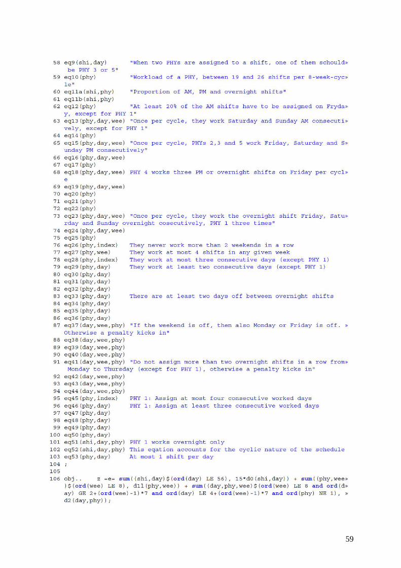
59

60

61

62

Reformulation

63

64

65

Expansion up to eight physicians

66

67

Schedules calculated with GAMS and NEOS Server for up to eight physicians

Table 22: Schedule for six physicians.

Table 23: Schedule for seven physicians.

Table 24: Schedule for eight physicians.

i j

1 2 3 4 5 6 7 8 9 10 11 12 13 14 15 16 17 18 19 20 21 22 23 24 25 26 27 28

1 5 5 1 6 6 - - 2 1 1 1 5 5 5 - 4 5 5 1 1 1 6 6 4 6 - 3 3

2 6 3 3 1 1 - - 3 2 4 4 - 2 2 2 6 4 2 5 4 4 - 5 5 4 6 5 5

3 2 2 4 4 4 5 5 5 3 6 6 6 - - 3 3 6 6 2 3 3 3 2 2 1 1 2 2

i j

29 30 31 32 33 34 35 36 37 38 39 40 41 42 43 44 45 46 47 48 49 50 51 52 53 54 55 56

1 - 3 3 4 2 2 2 3 4 4 6 1 - - 5 2 2 3 - 4 4 2 2 3 3 4 6 6

2 - 1 5 5 4 1 1 1 3 2 2 2 3 3 3 5 1 1 6 6 6 4 6 6 - 3 - -

3 - - 1 3 - 6 6 5 5 5 4 6 1 1 - 4 4 2 3 - - 5 5 1 1 1 4 4

i j

1 2 3 4 5 6 7 8 9 10 11 12 13 14 15 16 17 18 19 20 21 22 23 24 25 26 27 28

1 5 5 3 4 1 1 1 6 1 1 7 3 5 5 1 4 5 2 3 3 3 6 5+6 3 4 4 6 6

2 7 2 6 3 4 7 7 7 6 4 4 4 2 2 6 6 7 5 5 - - 7 1 1 3 2 1 1

3 4 7 2 6 3 5 5 2 2 6 1 7 3 3 2 1 4 7 2 4 4 4 7 5 5 3 2 2

i j

29 30 31 32 33 34 35 36 37 38 39 40 41 42 43 44 45 46 47 48 49 50 51 52 53 54 55 56

1 7 4 6 6 1 7 7 6 3 1 5 5 2 2 2 4 7 2+3 2 4 4 7 7 7 2 2 - -

2 5 5 2 2 2 5 5 7 2 3 4 7 3 3 6 5 1+5 1 1 6 6 4 3 3 1+3 6 4 4

3 1 7 4 3 3 1 1 5 6 2+6 1 1+4 7 7 3 6 4 7 3 - - 6 5 5 5 1 6 6

i j

1 2 3 4 5 6 7 8 9 10 11 12 13 14 15 16 17 18 19 20 21 22 23 24 25 26 27 28

1 4 3 8 2+8 5 5 5 6 6 2+3 3 4 4 4 5 5+7 7 4 1 1 1 3 7 1 4 4 7 7

2 7 6 6 1 2 4 4 4 5 1 1 1 8 8 3+8 2 8 5 4 6 6 8 8 7 6+8 6+8 2 2

3 1 4+7 3 6 1 3 3 8 7+8 5+7 2+7 2 6 6 6 3 2 7+8 5 2 2 6 3 3 1 5 5 5

i j

29 30 31 32 33 34 35 36 37 38 39 40 41 42 43 44 45 46 47 48 49 50 51 52 53 54 55 56

1 1 1+8 5 5 5 6 6 8 1 2+3 2+6 6 2 2 1 2 6+7 6 8 8 8 2 3 4+7 7 8 3 3

2 3 3 1 2 7 3 3 4 4 7 3+7 5 5 5 3 1+5 5 4+7 6 7 7 5 2 3+6 2+4 2 1 1

3 2 4 4+8 4+8 2 7 7 6 8 1 1 7 4 4 4 3 2+3 5 4 1 1 1 5 5 6 6 8 8

68

Excel spreadsheet (excerpt)

Original formulation

Ob

ject

ive

Sch

ed

ule

De

cisi

on

var

iab

les

De

viat

ion

var

iab

les

Au

xili

ary

vari

able

s

fun

ctio

nx i

jkd

0d

1/d

2s1

s2s3

/s4/

s5

12

34

5

lj i

12

31

23

12

31

23

12

31

23

12

31

23

45

12

34

51

23

45

12

34

5l

151

Mo

1-

-2

00

00

01

00

00

00

00

00

00

00

00

00

00

00

00

10

00

00

11

1

Tu2

--

50

00

00

00

00

00

00

01

00

00

00

00

00

00

10

10

00

11

11

02

Sum

We

34

-5

00

00

00

00

01

00

00

10

00

00

00

00

00

10

00

00

00

11

00

3

d-v

aria

ble

sTh

44

-1

00

10

00

00

01

00

00

00

00

00

00

01

00

00

00

00

10

10

11

4

d0

1Fr

54

21

00

10

10

00

01

00

00

00

00

00

00

00

10

00

00

00

01

01

11

5

d1

0Sa

63

21

00

10

10

10

00

00

00

00

00

00

00

00

01

00

00

00

01

11

01

6

d2

0Su

73

21

00

10

10

10

00

00

00

00

00

00

00

00

00

00

00

00

01

11

10

7

2M

o8

-3

50

00

00

00

10

00

00

01

00

00

00

00

00

00

11

00

00

10

00

18

Tu9

-4

50

00

00

00

00

01

00

01

00

00

00

00

00

01

00

00

00

00

00

0

We

10-

24

00

00

10

00

00

01

00

00

00

00

00

00

10

00

00

00

10

00

11

1

Th11

32

40

00

01

01

00

00

10

00

00

00

00

00

00

10

00

00

00

11

11

02

Fr12

3-

-0

00

00

01

00

00

00

00

00

00

00

00

00

00

00

00

10

01

10

03

Sa13

5-

-0

00

00

00

00

00

01

00

00

00

00

00

00

00

10

00

00

01

01

14

Su14

5-

-0

00

00

00

00

00

01

00

00

00

00

00

00

00

00

00

00

10

11

15

3M

o15

-5

40

00

00

00

00

00

10

10

00

00

00

00

00

01

00

00

00

11

10

16

Tu16

-2

40

00

01

00

00

00

10

00

00

00

00

00

01

00

00

00

00

11

11

07

We

17-

-2

00

00

01

00

00

00

00

00

00

00

00

00

00

00

00

01

01

00

01

8

Th18

3-

20

00

00

11

00

00

00

00

00

00

00

00

00

10

00

00

00

00

00

0

Fr19

35

10

01

00

01

00

00

00

10

00

00

00

00

10

00

10

10

00

00

11

11

Sa20

45

10

01

00

00

00

10

00

10

00

00

00

00

00

01

00

00

00

01

11

0

Su21

45

10

01

00

00

00

10

00

10

00

00

00

00

00

00

00

00

00

01

11

0

4M

o22

42

10

01

01

00

00

10

00

00

00

00

00

00

01

00

00

00

00

01

11

1

Tu23

-5

20

00

00

10

00

00

00

10

00

00

00

00

00

00

11

00

00

01

11

02

We

244

52

00

00

01

00

01

00

01

00

00

00

00

00

00

10

00

00

00

11

10

Th25

4-

50

00

00

00

00

10

00

01

00

00

00

00

00

00

00

10

00

01

10

1

Fr26

43

10

01

00

00

10

10

00

00

00

00

00

00

10

10

00

00

01

01

10

1

Sa27

-3

10

01

00

00

10

00

00

00

00

00

00

00

00

00

00

00

00

01

10

13

Su28

-3

10

01

00

00

10

00

00

00

00

00

00

00

00

00

00

00

00

01

10

1

5M

o29

5-

10

01

00

00

00

00

01

00

00

00

00

00

00

00

10

00

00

00

11

1

Tu30

54

30

00

00

00

01

01

01

00

00

00

00

00

00

11

01

00

00

00

11

1

We

31-

43

00

00

00

00

10

10

00

00

00

00

00

00

00

00

00

00

00

11

11

4

Th32

5-

40

00

00

00

00

00

11

00

00

00

00

00

00

00

10

01

00

00

11

1

Fr33

5-

20

00

00

10

00

00

01

00

00

00

00

00

01

00

00

00

10

00

11

1

min

1> 1>

1=

0=Bin

ary

69

Co

nst

rain

ts

Eq. N

o. 2

34+

56+

78

910

1112

13

RH

S≤

1≤

1≤

1≤

1≤

1≥

d0

23

45

= 0

12

34

51

23

45

12

34

51

23

45

12

31

23

12

34

51

23

12

31

23

12

31

23

45

l2

34

5

00

00

00

00

10

01

00

00

10

10

00

10

00

2424

1926

268

88

67

69

98

99

80

22

22

10

00

0

00

01

00

00

10

00

01

10

00

11

00

10

01

=≤

=2

00

00

00

01

00

00

10

00

01

10

10

11

10

10

01

2424

1926

268

88

77

79

99

99

90

22

22

30

00

0

00

01

00

01

00

11

01

01

11

00

10

10

00

≥4

00

00

01

10

00

11

00

11

10

01

11

00

11

10

00

88

86

66

88

88

88

50

00

0

01

10

00

10

00

11

10

01

01

00

11

11

00

60

00

0

01

00

00

10

00

10

10

01

00

10

11

11

00

70

00

0

00

10

00

01

00

00

01

10

10

01

01

10

11

80

00

0

00

01

00

01

10

01

00

10

11

01

01

10

01

01

10

00

11

00

01

11

00

01

10

01

10

00

01

10

00

10

01

00

11

00

00

11

11

11

00

00

00

10

00

01

00

00

10

00

01

10

01

00

00

00

10

00

00

00

00

10

00

01

10

01

00

00

00

00

00

00

00

00

10

10

00

10

01

00

00

00

10

00

01

01

01

00

00

10

01

10

10

01

00

00

11

00

00

01

00

01

10

01

10

00

00

10

00

01

00

01

10

00

11

01

00

10

00

00

10

00

00

10

01

10

10

10

11

10

11

00

00

01

10

00

11

10

01

11

00

11

11

11

10

00

01

10

00

11

10

01

11

10

10

11

10

10

00

01

10

00

01

11

01

01

00

01

11

10

10

01

00

00

10

10

10

00

11

00

11

11

10

00

00

01

10

00

11

01

01

10

10

10

01

10

10

00

01

10

00

11

01

01

00

11

10

11

10

10

00

01

00

00

00

00

11

10

01

01

10

10

01

00

10

00

01

00

10

10

01

01

00

11

10

10

00

10

00

01

01

10

10

01

00

01

01

10

10

00

10

10

01

01

10

00

11

00

11

01

10

10

00

00

10

00

00

10

01

11

00

10

10

11

00

00

01

00

00

11

00

11

00

01

01

11

11

01

00

01

10

00

11

00

10

10

01

01

01

10

01

00

00

10

00

00

00

01

10

00

10

10

11

00

00

00

00

00

00

01

00

00

10

00

10

11

00

1>1>

1>1>

1>

0=

==

<

><

70

1415

+16

173

1819

20-2

223

+24

2526

2728

29

=2=

0=

3≥

0=

0=

0≤

4≤

4≤

3≤

0

23

45

23

52

35

44

44

41

23

45

12

34

51

23

45

12

34

52

34

52

34

5

22

22

00

03

33

00

21

70

00

00

93

33

34

24

24

44

23

21

02

2-1

00

0

00

00

0=

==

00

00

0=

==

==

40

32

40

23

34

10

32

00

00

00

00

02

17

00

00

09

33

33

42

42

23

32

44

21

31

00

0-1

00

00

00

00

00

22

42

04

33

43

32

20

00

-10

00

00

00

00

00

02

22

21

32

34

33

11

00

-10

00

00

00

00

00

02

34

24

22

33

23

12

-10

00

00

01

00

00

00

24

42

24

32

33

22

22

-1-1

00

00

00

00

00

00

24

42

24

43

33

22

32

0-1

00

22

31

00

0-1

22

21

00

-10

12

12

-10

-10

01

13

0-1

00

10

23

00

00

20

22

00

0-1

31

21

00

0-1

32

11

00

-10

22

12

-10

00

12

23

-10

00

11

33

0-1

00

20

33

00

0-1

30

33

00

-1-1

30

33

00

-10

21

33

-10

00

12

32

-10

0-1

03

21

00

-1-1

03

11

00

-10

03

12

0-1

00

03

22

0-1

00

02

33

00

00

12

33

00

0-1

21

22

0-1

-10

30

12

00

-10

31

01

00

0-1

2=

==

3>0>

0=0<

0=0=

4>

3=

4>

71

3031

3233

3435

3637

/38

39

≤ 1

≥ 0

≤ 0

≤ 0

≤ 1

≥ 0

≤ 1

≤ 1

≥ 2

23

45

23

45

23

45

12

34

51

23

45

12

34

51

23

45

l1

23

45

l1

23

45

00

0-1

01

10

00

01

01

1Sa

11

11

11

22

22

2

10

01

10

00

00

-10

00

00

00

10

01

00

00

10

10

01

Su1

11

11

22

22

22

00

11

00

00

00

00

00

00

-10

00

01

00

00

01

00

00

2Sa

11

11

13

22

22

2

00

11

00

01

-10

-10

00

00

01

00

01

10

00

01

00

01

Su1

11

11

42

22

22

10

10

00

00

0-1

00

-10

00

01

00

00

00

00

01

00

00

3Sa

11

11

15

22

22

2

11

10

00

10

-10

00

-10

00

01

00

00

00

00

01

00

00

Su1

11

11

62

22

22

11

00

00

00

0-1

0-1

-10

00

01

00

00

00

00

00

00

01

4Sa

11

11

17

22

22

2

11

01

10

00

00

-10

00

00

01

00

01

00

00

11

00

01

Su1

11

11

82

22

22

01

11

01

00

-10

00

00

00

-10

00

01

00

00

00

00

10

5Sa

11

11

1

10

11

00

01

0-1

-10

00

00

00

00

11

00

01

00

00

11

Su1

11

11

11

10

00

00

00

00

00

0-1

00

00

10

00

00

00

00

00

6Sa

11

11

1

11

10

10

10

00

0-1

00

00

00

00

10

00

00

00

00

10

Su1

11

11

01

01

01

00

00

00

00

00

00

00

00

00

00

00

00

00

7Sa

11

11

1

00

01

00

00

00

-1-1

00

00

00

00

00

00

00

00

00

10

Su1

11

11

00

11

00

00

-10

00

00

00

00

00

10

00

01

00

00

10

8Sa

11

11

1

10

11

00

01

00

00

00

0-1

00

00

10

00

00

00

10

00

Su1

11

11

10

10

00

10

-1-1

00

00

00

00

10

10

01

00

00

10

10

11

00

00

00

00

0-1

0-1

00

00

10

00

00

00

01

00

00

11

01

10

00

00

-10

00

00

01

10

00

10

00

01

10

00

01

11

01

00

00

0-1

-10

00

01

00

00

00

00

01

00

00

00

11

00

00

-10

-10

-10

00

01

00

00

00

00

01

00

00

10

11

00

01

00

0-1

-10

00

01

00

00

00

00

00

10

00

10

11

00

10

-10

-10

00

00

01

10

00

01

00

01

10

00

10

11

00

00

00

0-1

0-1

00

00

10

00

00

00

00

00

01

10

11

10

00

0-1

-10

00

00

00

10

01

00

00

11

10

00

01

11

00

01

00

00

00

00

01

00

01

10

00

01

00

01

01

10

00

10

0-1

00

-10

00

01

00

00

00

00

01

00

00

01

00

00

00

00

0-1

-10

00

01

00

00

00

00

01

00

00

01

01

01

00

0-1

-10

-10

00

01

00

00

00

00

00

0-1

00

01

11

00

00

00

00

00

00

01

01

00

00

10

01

0-1

00

01

11

00

01

00

-1-1

00

-10

00

01

00

00

00

00

00

10

01

11

01

00

-10

00

00

00

00

01

10

00

01

00

11

00

10

11

00

10

00

00

00

00

00

10

10

01

00

00

10

10

1>0<

0>

0>

1>

0<

1>

1>

2<

72

4041

4243

4445

4647

4849

50

≤ 5

≤ 1

≤ 1

≥ 2

≥ 0

≤ 4

≤ 0

≤ 1

≥ 0

≤ 0

≤ 0

12

34

5l

23

45

23

45

23

45

23

45

11

11

11

33

35

52

00

0

44

55

31

Tu1

11

11

11

12

22

21

22

03

00

00

-1

45

53

3W

e1

11

11

11

12

22

22

22

04

00

0-1

-1

44

35

5Th

11

11

11

11

22

22

22

21

40

10

00

53

54

52

Tu1

11

11

11

12

22

22

21

03

-11

0-1

-1

55

53

4W

e1

11

11

11

12

22

22

20

12

-11

0-1

0

55

45

3Th

11

11

11

11

22

22

22

02

1-1

10

00

43

33

53

Tu1

11

11

11

12

22

21

20

20

01

10

0

We

11

11

11

11

22

22

02

12

00

00

00

Th1

11

11

11

12

22

20

22

20

00

00

0

4Tu

11

11

11

11

22

22

02

22

00

00

00

We

11

11

11

11

22

22

02

21

00

00

00

Th1

11

11

11

12

22

21

22

10

00

00

0

5Tu

11

11

11

11

22

22

20

22

00

00

00

We

11

11

11

11

22

22

20

12

10

00

00

Th1

11

11

11

12

22

21

11

22

00

00

0

6Tu

11

11

11

11

22

22

21

22

30

00

0-1

We

11

11

11

11

22

22

21

22

40

00

-1-1

Th1

01

11

11

12

22

22

21

24

01

00

0

7Tu

10

11

11

11

22

22

22

22

3-1

10

-1-1

We

11

11

11

11

22

22

22

22

2-1

10

-10

Th1

11

11

11

12

22

22

22

12

-11

00

0

8Tu

10

11

11

11

22

22

22

22

20

11

00

We

11

11

11

11

22

22

22

22

30

00

0-1

Th1

11

11

11

12

22

22

12

24

00

0-1

-1

40

10

00

3-1

10

-1-1

2-1

10

-10

1-1

10

00

00

11

00

00

00

00

10

00

00

20

00

00

1>1>

2<0<

4>0>

1>0<

0>0>

5>

73

Reformulation

Ob

ject

ive

De

cisi

on

var

iab

les

De

viat

ion

var

.C

on

stra

ints

fun

ctio

nx i

jkd

0d

1/d

2Eq

. No

. 2

3

12

34

5R

HS

≤ 1

≤ 1

lj i

12

31

23

12

31

23

12

31

23

12

31

23

45

l1

23

45

12

34

5

151

Mo

1-

51

00

10

00

00

00

00

01

00

00

00

00

01

00

00

10

01

01

Tu2

--

10

01

00

00

00

00

00

00

00

00

00

00

20

01

00

00

00

1

Sum

We

33

-1

00

10

00

10

00

00

00

00

00

00

00

03

00

00

10

00

01

d-v

aria

ble

sTh

45

31

00

10

00

01

00

00

10

00

00

00

00

04

00

10

10

01

00

d0

1Fr

55

24

00

00

10

00

00

01

10

00

00

00

00

05

01

00

00

10

00

d1

0Sa

6-

24

00

00

10

00

00

01

00

00

00

00

00

06

01

00

00

10

00

d2

0Su

7-

24

00

00

10

00

00

01

00

00

00

00

00

07

01

00

00

10

00

2M

o8

--

10

01

00

00

00

00

00

00

00

00

00

00

80

00

00

00

01

0

Tu9

-2

10

01

01

00

00

00

00

00

00

00

00

00

01

01

00

10

10

We

104

21

00

10

10

00

01

00

00

00

00

00

00

01

01

01

00

10

10

Th11

42

10

01

01

00

00

10

00

00

00

00

00

00

20

10

10

01

00

0

Fr12

43

50

00

00

00

10

10

00

01

00

00

00

00

30

01

00

00

10

0

Sa13

-3

50

00

00

00

10

00

00

01

00

00

00

00

40

01

00

00

10

0

Su14

-3

50

00

00

00

10

00

00

01

00

00

00

00

50

01

00

00

10

0

3M

o15

--

10

01

00

00

00

00

00

00

00

00

00

00

60

00

00

00

01

0

Tu16

-3

10

01

00

00

10

00

00

00

00

00

00

00

70

01

10

00

11

0

We

174

31

00

10

00

01

01

00

00

00

00

00

00

08

00

11

00

01

10

Th18

4-

10

01

00

00

00

10

00

00

00

00

00

00

00

01

00

00

00

Fr19

45

20

00

00

10

00

10

00

10

00

00

00

00

00

00

10

00

01

Sa20

-5

20

00

00

10

00

00

00

10

00

00

00

00

00

00

10

00

01

Su21

-5

20

00

00

10

00

00

00

10

00

00

00

00

00

00

10

00

11

4M

o22

--

30

00

00

00

01

00

00

00

00

00

00

00

00

01

00

10

00

Tu23

45

30

00

00

00

01

10

00

10

00

00

00

00

01

00

10

10

01

We

242

54

00

01

00

00

00

01

01

00

00

00

00

00

10

01

01

00

1

Th25

25

40

00

10

00

00

00

10

10

00

00

00

00

01

00

10

00

01

Fr26

2-

10

01

10

00

00

00

00

00

00

00

00

00

00

00

00

00

00

Sa27

--

10

01

00

00

00

00

00

00

00

00

00

00

00

00

00

00

00

Su28

--

10

01

00

00

00

00

00

00

00

00

00

00

00

00

00

00

01

5M

o29

-4

10

01

00

00

00

01

00

00

00

00

00

00

00

01

10

00

10

Tu30

54

20

00

00

10

00

01

01

00

00

00

00

00

00

01

00

00

10

We

31-

52

00

00

01

00

00

00

01

00

00

00

00

00

00

01

00

10

1

Th32

-4

50

00

00

00

00

01

00

01

00

00

00

00

00

11

00

01

10

Fr33

34

10

01

00

01

00

01

00

00

00

00

00

00

00

11

00

01

10

min

0=1>

1>1>

1=

Bin

ary

74

4r6r

89

1011

1213

1415

r

≤ 1

≤ 1

≤ 1

≥ d

02

34

5=

0=2

= 0

12

34

51

23

45

12

31

23

12

34

51

23

12

31

23

12

31

23

45

l2

34

52

34

52

35

10

00

01

01

00

01

10

10

2424

1926

268

88

67

69

98

99

80

22

22

10

00

02

22

20

00

10

10

01

01

01

00

10

00

=≤

=2

00

00

00

0

10

10

11

10

01

10

11

00

2424

1926

268

88

77

79

99

99

90

22

22

30

00

00

00

11

00

11

10

00

11

11

10

≥4

00

00

00

0

01

01

00

10

10

11

11

00

88

86

66

88

88

88

50

00

00

00

01

01

00

00

10

01

10

00

60

00

00

00

00

01

00

10

10

01

10

00

70

00

00

00

11

00

01

10

10

00

10

00

80

00

00

00

11

01

01

10

10

01

10

00

11

01

01

01

10

11

10

00

10

11

01

01

00

11

10

00

00

10

10

01

01

11

10

11

00

10

10

00

01

01

10

11

00

00

10

01

01

01

10

11

10

10

01

01

10

00

10

00

10

11

01

00

10

01

10

10

10

01

01

00

11

11

10

10

10

01

11

00

01

10

10

00

01

00

10

10

01

11

10

10

01

00

10

10

00

01

10

10

01

00

00

10

11

01

10

10

00

11

10

11

01

00

10

01

01

10

10

11

01

11

10

11

01

01

10

10

10

11

10

10

01

01

00

00

10

11

10

10

10

00

01

00

00

10

10

00

10

00

01

00

10

00

10

00

10

01

01

00

11

00

10

00

10

01

11

00

01

01

10

00

01

00

10

10

10

11

11

00

01

01

00

11

10

01

10

10

00

11

10

01

01

01

10

01

10

10

01

01

00

11

11

00

0=0=

1>

2=

< >

<

==

1>1>

75

1718

1920

22r

23r

2526

2728

29r

33r

= 3

≥ 0

= 0

=2=4

= 0

≤ 4

≤4≤

3≥

0≤

1

23

54

44

41

23

45

12

34

51

23

45

12

34

52

34

51

23

45

12

34

5

33

30

02

40

00

00

93

33

30

44

24

43

23

30

20

21

01

01

10

00

0

00

==

00

00

0=

==

==

22

40

44

33

33

12

12

10

00

11

00

00

00

24

00

00

09

33

33

42

30

24

32

33

22

22

01

01

00

00

10

00

00

00

04

04

20

33

23

33

13

21

01

00

10

00

0

10

00

00

04

24

40

42

34

33

03

10

10

11

00

01

0

00

00

00

02

23

42

13

24

33

02

01

00

00

10

00

0

00

00

00

02

44

42

44

24

43

02

00

20

10

00

01

0

00

00

00

00

24

24

03

32

43

02

01

00

10

10

00

0

31

31

11

00

01

00

00

22

32

00

11

10

00

01

13

23

11

00

01

00

00

03

13

00

11

10

00

01

03

02

10

00

01

00

00

03

11

00

20

10

00

01

02

20

10

01

01

00

00

12

31

10

00

01

00

00

21

32

01

11

10

10

00

30

23

10

00

01

00

00

31

13

01

01

10

10

00

22

13

00

10

00

01

00

22

23

01

01

20

10

00

22

33

01

00

00

00

10

31

33

00

11

10

01

00

30

22

11

00

01

00

00

20

11

00

01

10

00

10

10

10

11

00

01

00

00

10

21

10

01

01

00

00

20

22

01

00

10

10

00

20

33

10

00

01

00

00

21

33

00

02

10

00

01

12

22

11

10

01

10

0-1

03

21

00

00

10

00

01

03

10

10

11

01

00

00

3=

==

0<

0<0=

0=4>

4>

3>1>

=

76

37r

41rr

4546

r52

≤ 1

≤ 2

≤ 4

≤ 1

l1

23

45

23

45

11

23

45

11

-10

-11

00

00

40

00

01

21

0-1

1-1

00

00

31

00

00

30

-11

1-1

00

00

20

01

00

40

10

10

02

20

2-1

01

01

50

0-1

10

20

01

2-1

10

11

60

11

-11

00

22

30

10

10

7-1

-10

-11

21

00

41

10

10

81

1-1

0-1

10

12

40

00

00

31

10

00

20

10

10

2-1

10

10

2-1

01

11

30

01

01

41

01

01

40

00

00

31

01

00

20

01

10

1-1

00

10

00

10

11

00

10

01

00

10

01

10

01

00

2-1

01

11

30

10

11

41

10

11

40

10

00

31

00

00

20

00

00

2-1

00

10

2-1

10

11

30

10

01

41

00

11

40

01

10

2>

4>1>

1>

1>

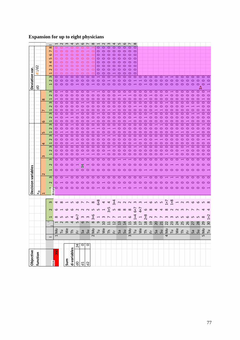
77

Expansion for up to eight physicians

Ob

ject

ive

De

cisi

on

var

iab

les

De

viat

ion

var

.

fun

ctio

nx i

jkd

0d

1/d

2

12

34

56

78

lj i

12

31

23

12

31

23

12

31

23

12

31

23

12

31

23

12

34

56

78

l

360

1M

o1

86

40

00

00

00

00

00

10

00

01

00

00

10

00

00

00

00

01

00

1

Tu2

51

80

10

00

00

00

00

01

00

00

00

00

00

10

00

00

00

00

00

2

Sum

We

35

61

00

10

00

00

00

00

10

00

10

00

00

00

00

00

00

00

00

13

d-v

aria

ble

sTh

44

65

00

00

00

00

01

00

00

10

10

00

00

00

00

00

00

00

00

04

d0

24Fr

54+

72

60

00

01

00

00

10

00

00

00

11

00

00

01

00

00

00

00

00

5

d1

0Sa

63

27

00

00

10

10

00

00

00

00

00

00

10

00

00

00

00

00

00

06

d2

0Su

73

27

00

00

10

10

00

00

00

00

00

00

10

00

00

00

00

00

01

07

2M

o8

3+6

58

00

00

00

10

00

00

01

01

00

00

00

01

10

00

00

00

00

18

Tu9

15

6+8

10

00

00

00

00

00

01

00

01

00

00

01

00

10

00

00

00

01

We

103

14

01

00

00

10

00

01

00

00

00

00

00

00

00

00

00

00

00

02

Th11

73+

54

00

00

00

01

00

01

01

00

00

10

00

00

01

00

00

00

00

03

Fr12

75

3+4

00

00

00

00

10

01

01

00

00

10

00

00

00

11

00

00

00

04

Sa13

18

21

00

00

10

00

00

00

00

00

00

00

01

00

00

00

00

00

00

5

Su14

18

21

00

00

10

00

00

00

00

00

00

00

01

00

00

00

00

00

00

6

3M

o15

68

20

00

00

10

00

00

00

00

10

00

00

01

00

00

00

00

00

00

7

Tu16

1+4

6+7

31

00

00

00

01

10

00

00

01

00

10

00

01

10

00

00

00

00

8

We

171

4+7

31

00

00

00

01

01

00

00

00

00

10

00

00

10

00

00

00

00

Th18

2+8

61

00

11

00

00

00

00

00

00

10

00

01

00

10

00

00

00

00

0

Fr19

28

60

00

10

00

00

00

00

00

00

10

00

01

00

00

00

00

00

00

Sa20

74

50

00

00

00

00

01

00

01

00

01

00

00

00

00

00

00

00

00

Su21

74

50

00

00

00

00

01

00

01

00

01

00

00

00

00

00

00

00

00

4M

o22

38

1+7

00

10

00

10

00

00

00

00

00

00

10

10

00

10

00

00

00

0

Tu23

32

1+8

00

10

10

10

00

00

00

00

00

00

00

01

00

10

00

00

00

0

We

245

21

00

10

10

00

00

00

10

00

00

00

00

00

00

00

00

00

00

0

Th25

53

20

00

00

10

10

00

01

00

00

00

00

00

00

00

00

00

00

00

Fr26

67

30

00

00

00

01

00

00

00

10

00

10

00

00

00

00

00

00

00

Sa27

57

60

00

00

00

00

00

01

00

00

10

10

00

00

00

00

00

00

00

Su28

57

60

00

00

00

00

00

01

00

00

10

10

00

00

00

00

00

00

00

5M

o29

84

50

00

00

00

00

01

00

01

00

00

00

10

00

00

00

00

00

00

Tu30

1+2

48

10

01

00

00

00

10

00

00

00

00

00

01

10

00

00

00

00

0

min

1>

1=

Bin

ary

78

Co

nst

rain

ts

Eq. N

o.

23

4r6r

810

e11

e13

e

RH

S≤

1≤

1≤

1≤

1≤

1=2

4=8

= 0

12

34

56

78

12

34

56

78

12

34

56

78

12

34

56

78

12

31

23

45

67

8k

12

3k

l1

23

00

00

11

00

00

00

11

00

10

01

10

00

00

01

11

00

11

124

2424

2424

2424

241

88

81

10

00

10

00

10

00

10

01

00

00

00

00

11

01

00

01

01

01

11

12

88

82

00

0

00

01

01

00

00

01

01

10

10

01

01

00

11

01

00

10

11

13

88

83

00

0

00

01

01

10

00

10

01

00

01

01

10

10

01

10

10

00

11

14

88

84

00

0

01

10

00

00

01

10

00

00

01

10

01

00

01

10

01

00

11

15

88

85

00

0

01

10

00

00

01

10

01

00

01

10

00

10

00

10

11

10

11

16

88

86

00

0

01

10

01

00

11

00

00

00

00

10

11

10

10

00

10

10

11

17

88

87

00

0

10

00

10

00

00

10

10

00

10

00

10

01

10

10

00

01

11

18

88

88

00

0

00

10

10

00

00

00

10

10

10

10

01

01

00

10

11

11

11

12

10

00

10

00

00

10

10

00

00

10

00

11

10

10

00

01

10

10

11

12

00

0

00

10

10

10

10

10

10

00

00

01

10

10

10

01

00

01

11

13

00

0

10

00

10

00

10

00

10

00

10

11

00

01

10

11

00

01

11

14

00

0

10

00

00

01

00

00

01

01

11

00

00

01

01

00

01

01

11

15

00

0

00

00

01

01

10

01

00

01

01

00

01

01

11

01

01

10

11

16

00

0

10

01

00

01

10

00

00

01

11

01

01

10

11

01

00

10

11

17

00

0

10

00

01

10

01

00

01

11

10

11

00

10

01

10

01

01

11

18

00

0

01

01

00

11

01

01

00

10

01

10

01

01

01

10

00

01

11

13

10

00

01

00

01

00

00

00

01

10

11

00

00

01

10

01

00

10

11

12

00

0

00

00

00

11

00

00

00

11

00

01

01

10

00

01

01

10

11

13

00

0

00

01

00

10

00

11

00

00

00

01

10

10

00

10

10

01

11

14

00

0

00

11

00

00

00

11

00

00

00

10

10

01

01

10

10

00

11

15

00

0

00

10

00

01

00

00

10

01

11

10

00

10

11

00

10

10

11

16

00

0

01

00

10

00

01

00

10

00

11

00

10

01

10

10

10

01

11

17

00

0

01

00

10

00

01

00

01

00

10

10

10

00

10

00

01

10

11

18

00

0

00

10

01

00

00

10

10

00

01

00

01

10

01

00

10

10

11

14

10

00

00

00

10

10

00

00

10

10

00

10

10

10

00

10

10

10

11

12

00

0

00

00

10

10

00

00

00

11

00

00

11

10

00

01

01

01

11

13

00

0

00

00

00

11

11

00

00

10

00

01

01

01

11

01

01

00

11

14

00

0

11

01

00

00

10

01

00

10

11

01

10

00

11

10

10

10

11

15

00

0

10

01

00

10

00

01

10

10

11

10

00

11

10

10

10

11

11

16

00

0

1>1>

1>

8=

24=

1>1>

79

14e

2627

2829

r33

r37

r

=2≤

4≤4

≤ 3

≥ 0

≤ 1

≤ 1

k1

23

12

34

56

78

12

34

56

78

12

34

56

78

12

34

56

78

12

34

56

78

l1

23

45

67

8

12

22

24

42

20

42

23

23

34

32

20

02

33

02

00

01

02

00

10

01

00

0-1

10

-1-1

11

1-1

1

22

22

22

42

42

42

42

43

42

24

21

02

33

11

00

01

10

01

-10

00

10

01

2-2

-11

11

11

-1

32

22

02

42

44

40

33

24

24

43

12

12

23

20

11

00

01

10

10

00

-11

00

31

11

-2-2

1-1

1

42

22

22

40

44

22

33

40

43

42

03

22

12

30

00

10

10

00

00

00

1-1

10

40

01

1-1

-1-1

1

52

22

42

42

22

04

34

44

33

33

03

31

12

31

01

01

01

10

00

00

01

00

51

-1-2

11

-11

1

62

22

40

44

22

04

43

23

42

24

12

30

22

22

00

10

11

01

00

00

00

01

6-1

11

1-2

01

-1

72

22

22

44

02

22

32

24

22

44

21

31

22

12

11

00

00

10

00

00

01

10

7-2

11

-10

01

-1

82

22

24

42

02

22

24

43

24

22

20

32

32

12

00

21

00

00

00

01

0-1

00

81

1-2

-10

-10

1

20

33

31

21

00

00

21

11

00

00

01

01

21

33

20

21

10

11

00

00

00

11

00

00

22

22

20

22

11

00

00

01

01

-10

00

00

23

11

11

13

00

11

10

10

00

11

00

00

33

11

02

13

01

00

01

01

01

00

00

00

32

22

02

22

20

11

00

10

00

10

00

00

32

22

03

22

01

00

00

01

01

00

00

00

32

22

03

22

11

00

02

01

10

00

00

00

22

12

12

22

00

11

00

10

-10

10

01

00

12

02

22

22

10

01

10

10

10

00

1-1

00

11

12

21

32

01

00

01

01

00

00

01

00

21

22

20

32

10

10

00

11

10

00

00

10

32

21

20

22

01

01

10

00

00

00

10

-11

33

30

20

12

10

00

10

10

10

00

00

1-1

23

30

21

11

01

20

00

01

01

00

00

01

12

20

32

20

10

00

01

10

1-1

10

00

00

01

20

33

30

01

00

20

00

01

-10

01

00

00

11

33

31

00

10

01

10

00

10

00

00

11

02

32

22

00

01

10

01

00

00

10

00

22

12

21

23

11

00

01

10

00

00

-11

01

32

23

20

23

00

10

10

11

00

00

10

00

32

23

21

32

10

02

10

00

00

01

00

00

0<

4>4>

3>1>

1>2=

80

41rr

5253

≤ 2

≥ 1

≤ 1

12

34

56

78

12

31

23

45

67

8

10

01

10

01

11

10

00

10

10

1

00

02

01

02

11

11

00

01

00

1

11

20

00

00

11

11

00

01

10

0

21

00

00

11

11

10

00

11

10

0

00

01

10

02

21

10

10

10

11

0

01

10

02

20

11

10

11

00

01

0

12

00

21

00

11

10

11

00

01

0

00

00

20

20

21

10

01

01

10

1

11

21

00

01

10

1

11

11

01

10

00

0

12

10

01

11

01

0

11

20

01

11

01

0

11

11

10

00

00

1

11

11

10

00

00

1

11

10

10

00

10

1

22

11

01

10

11

0

12

11

01

10

01

0

21

11

10

00

10

1

11

10

10

00

10

1

11

10

00

11

01

0

11

10

00

11

01

0

11

21

01

00

01

1

11

21

11

00

00

1

11

11

10

01

00

0

11

10

11

01

00

0

11

10

01

00

11

0

11

10

00

01

11

0

11

10

00

01

11

0

11

10

00

11

00

1

21

11

10

10

00

1

2>

1>1<

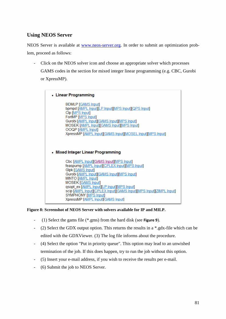
81

Using NEOS Server

NEOS Server is available at www.neos-server.org. In order to submit an optimization prob-

lem, proceed as follows:

- Click on the NEOS solver icon and choose an appropriate solver which processes

GAMS codes in the section for mixed integer linear programming (e.g. CBC, Gurobi

or XpressMP).

Figure 8: Screenshot of NEOS Server with solvers available for IP and MILP.

- (1) Select the gams file (*.gms) from the hard disk (see Figure 9).

- (2) Select the GDX output option. This returns the results in a *.gdx-file which can be

edited with the GDXViewer. (3) The log file informs about the procedure.

- (4) Select the option "Put in priority queue". This option may lead to an unwished

termination of the job. If this does happen, try to run the job without this option.

- (5) Insert your e-mail address, if you wish to receive the results per e-mail.

- (6) Submit the job to NEOS Server.

82

Figure 9: The input page on NEOS server.

Sometimes, NEOS does not automatically forward from the solving screen to the result

screen. In this case, the results for the job can be fetched by a query:

- Note the job number and password (see Figure 10).

- Go to the initial Homepage of NEOS and click on "view current job queues" (see Fig-

ure 11).

- Insert the job number and password and select "View Job Results" (see Figure 12).

Figure 10: Solver screen of NEOS with job-number and password for a query.

83

Figure 11: Main screen of NEOS Server with the query option.

Figure 12: Query screen on NEOS.

84

Installation hints for OpenSolver

OpenSolver is downloaded as a .zip file on http://opensolver.org/installing-opensolver. After

extracting the .zip file on the hard disk, double-click on the add-in OpenSolver.xlam. Excel is

opened and OpenSolver shows up in the data toolbar. Make sure to activate the macros when

asked to do so.

In order to activate the OpenSolver add-in permanently, open the options in the file tab and

choose the add-ins category. At the bottom of the dialog box, make sure that Excel add-ins is

selected in the Manage box and click "Go". Select "Browse…" and choose the OpenSolver

add-in. At the next start of Excel, OpenSolver shows up automatically.30

30

The installation hints are for Microsoft Excel 2010. Add-in settings may differ in other versions.

85

Using OpenSolver

The following user advices require basic knowledge in linear programming and Excel's stand-

ard solver from Frontline.

OpenSolver provides some options (see Figure 13): The calculation time can be limited, either

with the maximum solution time in seconds or with the branch and bound tolerance in per-

cent. With a tolerance of 100%, OpenSolver stops at the first found feasible integer solution.

A tolerance of 50% means that OpenSolver terminates the branch and bound algorithm as

soon as the optimal LP relaxation value is within the range of the best solution found so far

(the incumbent) plus/minus 50%. In a setting with an optimal value of 15 and a tolerance of

50%, the solver stops as soon as the incumbent is 30 or lower. If the tolerance is only 20%,

the solver does not stop before the incumbent is 18 or lower.

The Quick AutoModel was not tested in the present thesis, since the scheduling model is too

comprehensive for this tool.

Figure 13: The Open solver module in the data tab (left) and solve options.

A handicap of OpenSolver is illustrated in Figure 14: Compared to the Excel's standard solv-

er, OpenSolver does not support range names. Although new constraints can be added by us-

ing range names, but the names are not displayed in the constraint overview. On the other

hand, the constraints can be highlighted graphically in the spreadsheet (see Figure 15). This

feature is activated by the option "Show model after saving" in the model dialog box or by the

icon "Show/Hide Model" in the OpenSolver toolbar. When the model is set up, you can click

on the icon "Solve" in the toolbar and OpenSolver starts the calculation.

86

Figure 14: Model dialog box.

Figure 15: OpenSolver emphasizes in color the model.

87

Figure 16: OpenSolver menu with Quick Solve.

The OpenSolver icon in the toolbar allows to solve the LP relaxation of an IP or to use Quick

Solve. Quick Solve is useful tool if a model is repeatedly solved with some parameters chang-

ing. After choosing the modifiable parameters and initializing Quick Solve, OpenSolver

should provide the solution with the changed parameters in a short time. Unfortunately, Quick

Solve did not accelerate the computation time of the scheduling model.

.

88

E-Mail exchange with Yann Ferrand

Mail to Yann Ferrand on April 29, 2012:

Dear Mister Ferrand

I am writing my master thesis at the chair of Karl Schmedders, Professor of Quantitative

Business Administration at the University of Zurich. One goal of my thesis is to find out

whether the open-source-software OpenSolver for Excel is able to solve large Integer Pro-

grams IP. In search of an appropriate problem in academic literature I found your paper and

modeled it in Excel.

To my surprise, OpenSolver found a solution with a z-value (objective function) of 0 in less

than two hours.

Additionally, I modeled your IP with GAMS and solved it on the NEOS-Server. NEOS-

Server calculates the solution within seconds! The distribution of the shifts is different to the

solution in OpenSolver. However, the z-value of the objective function is 0 again.

Both solutions account the fact that the end of one cycle is connected to the beginning of the

subsequent cycle.

I wonder why I get a different solution compared to yours; and have two possible explana-

tions: (1) I made wrong assumptions or (2) there are additional constraints not mentioned in

the paper. May you have an idea for the different results?

These are basically the assumptions made:

- I merged equations 4 and 5 to x3jk + x1(j+1)k + x2(j+1)k ≤ 1

If physician k works overnight, he or she does not work AM and PM the next day. And if he

does not work overnight, he or she works one shift at most the next day. Therefore, the sum of

the three variables is always less or equal 1.

- Equations 6 and 7 are merged in the same way.

- Equation 10: Physicians 1 and 2 work 24 shifts per cycle, physician 3 works 19 shifts and

physicians 4 and 5 work 26 shifts (I counted the number of shifts in Table 1 in your paper).

- Equation 11: The upper bound is 9 (except for physician 3: 7).

Both my solutions (with OpenSolver and GAMS) are attached.

89

I would be glad if my thesis could support your enhancement of the cyclic schedule, as you

describe in the conclusion-section, and hope to receive a favorable answer.

Answer from Yann Ferrand on May 5, 2012:

Thank you very much for your email, I am thrilled that you are interested in this problem.

Regarding your assumptions:

1) I don't suspect merging equations 4 and 5, and 6 and 7 is a problem.

2) For equation 10, you are correct: the right hand side (RHS) is respectively for physicians 1

through 5: 24, 24, 19, 26 and 26.

3) For equation 11, I think this is where you have an issue: there is both upper and lower

bound. Physician 1 is mentioned in the article (all 24 shifts are night shifts), for physician 2

the bounds are 8 and 8; for physician 3 they are 6 and 7; and physicians 4 and 5 they are 8 and

9. For all but physician 1, these same bounds apply for day/evening/night shifts.

Now, in your GAMS file solution (edits attached), I see that physician 2 is working 6 night

shifts, and physician 3 is working 5 night shifts. This is not enough. Right now I cannot recall

the exact reason why, but I remember that it was impossible to avoid assigning 2 physicians

to some of the night shifts, the reason has to do with the number of night slots available, and

the minimum requirements for night shifts for all the physicians.

I would rerun your formulation with those lower bounds for the number of shifts of each type,

and see what you get.

Another precision: in several instances I tried I could get a feasible solution in a few hours by

terminating the search (my objective would not be 0, and the solver would keep searching).

I look forward to hearing from you about your progress.

Mail to Yann Ferrand on May 7, 2012:

Thank you so much for your helpful answer. I really forgot about equation 11 and did not

check the lower bound of the distribution of the different shifts. I guess that after implement-

ing the lower bounds, the new optimal z-value should be 15, which means that exactly one

overnight shift is assigned to 2 physicians. The reason for this is in equation 25: each physi-

90

cian is assigned to work overnight shifts at exactly one weekend (3 weekends for physician

1); hence 7 (3 + 4*1) weekends are covered with overnight shifts. In total, there are at least 54

overnight shifts to be assigned (24 + 8 + 6 + 8 + 8, in accordance with the lower bounds) but

only 53 overnight shifts can be assigned due to equation 25 (56 – 3; one weekend is not cov-

ered). As soon as my new solution is beyond the shadow of a doubt I’ll send you the new re-

sults.

Another issue: I am reformulating equations 29 to 44 and 46 to 50 eliminating the s-variables

(and ignoring your hint of a tight problem formulation). Please find attached a file with a pos-

sible reformulation.

Answer from Yann Ferrand on May 8, 2012:

You are correct on your reasoning about the number of night shifts and the weekend night

shifts assignments, that's what I was trying to remember the other day. Now, the reason we

went with the solution in the paper as opposed to one where there is only 1 shift with double

assignments is that the physicians liked this particular solution we proposed.

Also, the tight problem formulation may not be a big issue in this instance with 5 physicians,

but with 6 physicians it helps. Also, with 7 and 8 physicians I could not get solutions with this

formulation.

Let me know what kind of solutions you get once you have them, it would be great if you

were able to generate good solutions with the open solver!

Mail to Yann Ferrand on July 18, 2012:

I got stuck a bit at the theory section of my thesis. One point remains unclear to me: Open-

Solver indeed passes through much fewer nodes (9,030 nodes) with your formulation with the

s-variables, compared to the formulation without the s-variables (39,000 nodes!). Anyway,

the solution time with OpenSolver is similar with both approaches: the optimal solution of 15

is obtained within 45 minutes with the s-variables and within 52 minutes without the s-

variables.

As a “goodie” in my thesis I formulated the problem with 6 and 7 physicians and received an

optimal solution using NEOS-server (with a GAMS input).

91

I’ll gladly send you a copy of the thesis by end of August.

Answer from Yann Ferrand on July 19, 2012:

Thank you for the update. This is good news that you found a solution for bigger size prob-

lems. The formulation with the s-variables prevents some x-variables from taking a value of

½, which then lead to more branching.

92

Avoided constraints due to reformulation

Section 0 claims that 2,152 constraints can be eliminated by the formulation without s-

variables. The following table gives an explanation of this number:

group of

equations

# of constraints in original problem # of constraints in reformulation

29-32 4eq * 4ph * 56d = 896 1eq * 4ph * 56d = 224

33-36 4eq * 5ph * 56d = 1,120 1eq * 5ph * 56d = 280

37-40 4eq * 5ph * 8w = 160 1eq * 5ph * 8w = 40

41-44 4eq * 4ph * 3d * 8w = 384 1eq * 4ph * 8w = 32

46-50 5eq * 1ph * 56d = 280 2eq31

* 1ph * 56d = 112

∑ 2,840 688

Table 25: Number of constraints in the original and modified version.32

The original formulation contains 2,152 constraints more than the reformulation.

31

It is only one new equation (56 constraints). But this equation requires that equation (29r) must hold also for

physician 1. Therefore, the reformulation of equations (46) to (50) results in 112 constraints. 32

The abbreviations stand for: eq: equations, ph: physicians, d: days, w: weeks

93

Statutory declaration

I herewith declare that I have completed the present thesis independently making use only of

the specified literature and aids. Sentences or parts of sentences quoted literally are marked as

quotations; identification of other references with regard to the statement and scope of the

work is quoted. The thesis in this form or in any other form has not been submitted to an ex-

amination body and has not been published.

Date: _______________________ Signature: ______________________