solving big data challenges for enterprise application ... · solving big data challenges for...
TRANSCRIPT
Solving Big Data Challenges for Enterprise ApplicationPerformance Management
Tilmann RablMiddleware Systems
Research GroupUniversity of Toronto, Canada
Mohammad SadoghiMiddleware Systems
Research GroupUniversity of Toronto, Canada
Hans-Arno JacobsenMiddleware Systems
Research GroupUniversity of Toronto, Canada
[email protected] Gomez-Villamor
DAMA-UPCUniversitat Politecnica de
Catalunya, Spain
Victor Muntes-MuleroCA Labs EuropeBarcelona, Spain
Serge MankovskiiCA Labs
San Francisco, [email protected]
ABSTRACTAs the complexity of enterprise systems increases, the need formonitoring and analyzing such systems also grows. A number ofcompanies have built sophisticated monitoring tools that go far be-yond simple resource utilization reports. For example, based oninstrumentation and specialized APIs, it is now possible to monitorsingle method invocations and trace individual transactions acrossgeographically distributed systems. This high-level of detail en-ables more precise forms of analysis and prediction but comes atthe price of high data rates (i.e., big data). To maximize the benefitof data monitoring, the data has to be stored for an extended periodof time for ulterior analysis. This new wave of big data analyticsimposes new challenges especially for the application performancemonitoring systems. The monitoring data has to be stored in a sys-tem that can sustain the high data rates and at the same time enablean up-to-date view of the underlying infrastructure. With the ad-vent of modern key-value stores, a variety of data storage systemshave emerged that are built with a focus on scalability and high datarates as predominant in this monitoring use case.
In this work, we present our experience and a comprehensiveperformance evaluation of six modern (open-source) data stores inthe context of application performance monitoring as part of CATechnologies initiative. We evaluated these systems with data andworkloads that can be found in application performance monitor-ing, as well as, on-line advertisement, power monitoring, and manyother use cases. We present our insights not only as performanceresults but also as lessons learned and our experience relating tothe setup and configuration complexity of these data stores in anindustry setting.
1. INTRODUCTIONLarge scale enterprise systems today can comprise complete data
centers with thousands of servers. These systems are heteroge-neous and have many interdependencies which makes their admin-istration a very complex task. To give administrators an on-lineview of the system health, monitoring frameworks have been de-veloped. Common examples are Ganglia [20] and Nagios [12].These are widely used in open-source projects and academia (e.g.,Wikipedia1). However, in industry settings, in presence of stringentresponse time and availability requirements, a more thorough viewof the monitored system is needed. Application Performance Man-agement (APM) tools, such as Dynatrace2, Quest PerformaSure3,AppDynamics4, and CA APM5 provide a more sophisticated viewon the monitored system. These tools instrument the applicationsto retrieve information about the response times of specific servicesor combinations of services, as well as about failure rates, resourceutilization, etc. Different monitoring targets such as the responsetime of a specific servlet or the CPU utilization of a host are usu-ally referred to as metrics. In modern enterprise systems it is notuncommon to have thousands of different metrics that are reportedfrom a single host machine. In order to allow for detailed on-lineas well as off-line analysis of this data, it is persisted at a cen-tralized store. With the continuous growth of enterprise systems,sometimes extending over multiple data centers, and the need totrack and report more detailed information, that has to be stored forlonger periods of time, a centralized storage philosophy is no longerviable. This is critical since monitoring systems are required to in-troduce a low overhead – i.e., 1-2% on the system resources [2]– to not degrade the monitored system’s performance and to keepmaintenance budgets low. Because of these requirements, emerg-ing storage systems have to be explored in order to develop an APMplatform for monitoring big data with a tight resource budget andfast response time.
1Wikipedia’s Ganglia installation can be accessed at http://ganglia.wikimedia.org/latest/.2Dynatrace homepage - http://www.dynatrace.com3PerformaSure homepage - http://www.quest.com/performasure/4AppDynamics homepage - http://www.appdynamics.com5CA APM homepage - http://www.ca.com/us/application-management.aspx
1724
Permission to make digital or hard copies of all or part of this work forpersonal or classroom use is granted without fee provided that copies arenot made or distributed for profit or commercial advantage and that copiesbear this notice and the full citation on the first page. To copy otherwise, torepublish, to post on servers or to redistribute to lists, requires prior specificpermission and/or a fee. Articles from this volume were invited to presenttheir results at The 38th International Conference on Very Large Data Bases,August 27th - 31st 2012, Istanbul, Turkey.Proceedings of the VLDB Endowment, Vol. 5, No. 12Copyright 2012 VLDB Endowment 2150-8097/12/08... $ 10.00.
arX
iv:1
208.
4167
v1 [
cs.D
B]
21
Aug
201
2
APM has similar requirements to current Web-based informa-tion systems such as weaker consistency requirements, geograph-ical distribution, and asynchronous processing. Furthermore, theamount of data generated by monitoring applications can be enor-mous. Consider a common customer scenario: The customer’s datacenter has 10K nodes, in which each node can report up to 50Kmetrics with an average of 10K metrics. As mentioned above, thehigh number of metrics result from the need for a high-degree ofdetail in monitoring, – an individual metric for response time, fail-ure rate, resource utilization, etc. of each system component canbe reported. In the example above, with a modest monitoring in-terval of 10 seconds, 10 million individual measurements are re-ported per second. Even though a single measurement is small insize, below 100 bytes, the mass of measurements poses similar bigdata challenges as those found in Web information system applica-tions such as on-line advertisement [9] or on-line analytics for so-cial Web data [25]. These applications use modern storage systemswith focus on scalability as opposed to relational database systemswith a strong focus on consistency. Because of the similarity ofAPM storage requirements to the requirements of Web informa-tion system applications, obvious candidates for new APM storagesystems are key-value stores and their derivatives. Therefore, wepresent a performance evaluation of different key-value stores andrelated systems for APM storage.
Specifically, we present our benchmarking effort on open sourcekey-value stores and their close competitors. We compare the throu-ghput of Apache Cassandra, Apache HBase, Project Voldemort,Redis, VoltDB, and a MySQL Cluster. Although, there would havebeen other candidates for the performance comparison, these sys-tems cover a broad area of modern storage architectures. In contrastto previous work (e.g., [7, 23, 22]), we present details on the maxi-mum sustainable throughput of each system. We test the systems intwo different hardware setups: (1) a memory- and (2) a disk-boundsetup.
Our contributions are threefold: (1) we present the use case andbig data challenge of application performance management andspecify its data and workload requirements; (2) we present an up-to-date performance comparison of six different data store archi-tectures on two differently structured compute clusters; and, (3)finally, we report on details of our experiences with these systemsfrom an industry perspective.
The rest of the paper is organized as follows. In the next section,we describe our use case: application performance management.Section 3 gives an overview of the benchmarking setup and thetestbed. In Section 4, we introduce the benchmarked data stores. InSection 5, we discuss our benchmarking results in detail. Section 6summarizes additional findings that we made during our bench-marking effort. In Section 7, we discuss related work before con-cluding in Section 8 with future work.
2. APPLICATION PERFORMANCE MAN-AGEMENT
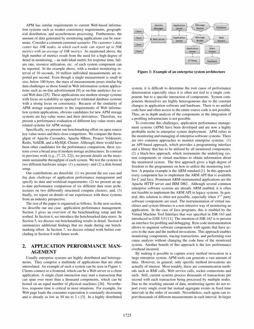
Usually enterprise systems are highly distributed and heteroge-neous. They comprise a multitude of applications that are ofteninterrelated. An example of such a system can be seen in Figure 1.Clients connect to a frontend, which can be a Web server or a clientapplication. A single client interaction may start a transaction thatcan span over more than a thousand components, which can behosted on an equal number of physical machines [26]. Neverthe-less, response time is critical in most situations. For example, forWeb page loads the consumer expectation is constantly decreasingand is already as low as 50 ms to 2 s [3]. In a highly distributed
Application
server Database
Client
Identity
Manager
Message
Queue
Client
Client
ClientWeb server
Application
server
Application
server
Database
Web
Service
Main
Frame
3rd Party
Message
Broker
Figure 1: Example of an enterprise system architecture
system, it is difficult to determine the root cause of performancedeterioration especially since it is often not tied to a single com-ponent, but to a specific interaction of components. System com-ponents themselves are highly heterogeneous due to the constantchanges in application software and hardware. There is no unifiedcode base and often access to the entire source code is not possible.Thus, an in depth analysis of the components or the integration ofa profiling infrastructure is not possible.
To overcome this challenges, application performance manage-ment systems (APM) have been developed and are now a highlyprofitable niche in enterprise system deployment. APM refers tothe monitoring and managing of enterprise software systems. Thereare two common approaches to monitor enterprise systems: (1)an API-based approach, which provides a programming interfaceand a library that has to be utilized by all monitored components;(2) a black-box approach, which instruments the underlying sys-tem components or virtual machines to obtain information aboutthe monitored system. The first approach gives a high degree offreedom to the programmer on how to utilize the monitoring tool-box. A popular example is the ARM standard [1]. In this approachevery component has to implement the ARM API that is availablefor C and Java. Prominent ARM-instrumented applications are theApache HTTP server and IBM DB2. Although several commonenterprise software systems are already ARM enabled, it is oftennot feasible to implement the ARM API in legacy systems. In gen-eral, this solution is often not possible, especially when 3rd partysoftware components are used. The instrumentation of virtual ma-chines and system libraries is a non-intrusive way of monitoring anapplication. In the case of Java programs, this is enabled by theVirtual Machine Tool Interface that was specified in JSR-163 andintroduced in J2SE 5.0 [11]. The intention of JSR-163 is to presentan interface for profiling and debugging. Byte code instrumentationallows to augment software components with agents that have ac-cess to the state and the method invocations. This approach enablesmonitoring components, tracing transactions, and performing rootcause analysis without changing the code base of the monitoredsystem. Another benefit of this approach is the low performanceoverhead incurred.
By making it possible to capture every method invocation in alarge enterprise system, APM tools can generate a vast amount ofdata. However, in general, only specific method invocations areactually of interest. Most notably, these are communication meth-ods such as RMI calls, Web service calls, socket connections andsuch. Still, current systems process thousands of transactions persecond with each transaction being processed by multiple nodes.Due to the resulting amount of data, monitoring agents do not re-port every single event but instead aggregate events in fixed timeintervals in the order of seconds. Nevertheless, each agent can re-port thousands of different measurements in each interval. In larger
1725
deployments, i.e., hundreds to thousands of hosts, this results in asustained rate of millions of measurements per second. This in-formation is valuable for later analysis and, therefore, should bestored in a long-term archive. At the same time, the most recentdata has to be readily available for on-line monitoring and for gen-erating emergency notifications. Typical requirements are slidingwindow aggregates over the most recent data of a certain type ofmeasurement or metric as well as aggregates over multiple metricsof the same type measured on different machines. For instance twotypical on-line queries are:
• What was the maximum number of connections on host Xwithin the last 10 minutes?
• What was the average CPU utilization of Web servers of typeY within the last 15 minutes?
For the archived data more analytical queries are as follows:
• What was the average total response time for Web requestsserved by replications of servlet X in December 2011?
• What was maximum average response time of calls from ap-plication Y to database Z within the last month?
While the on-line queries have to be processed in real-time, i.e.,in subsecond ranges, historical queries may finish in the order ofminutes. In comparison to the insertion rate, these queries are how-ever issued rarely. Even large clusters are monitored by a modestnumber of administrators which makes the ad-hoc query rate rathersmall. Some of the metrics are monitored by certain triggers thatissue notifications in extreme cases. However, the overall writeto read ratio is 100:1 or more (i.e., write-dominated workloads).While the writes are simple inserts, the reads often scan a small setof records. For example, for a ten minute scan window with 10seconds resolution, the number of scanned values is 60.
An important prerequisite for APM is that the performance of themonitored application should not be deteriorated by the monitoring(i.e., monitoring should not effect SLAs.) As a rule of thumb, amaximum tolerable overhead is five percent, but a smaller rate ispreferable. This is also true for the size of the storage system. Thismeans that for an enterprise system of hundreds of nodes only tensof nodes may be dedicated to archiving monitoring data.
3. BENCHMARK AND SETUPAs explained above, the APM data is in general relatively simple.
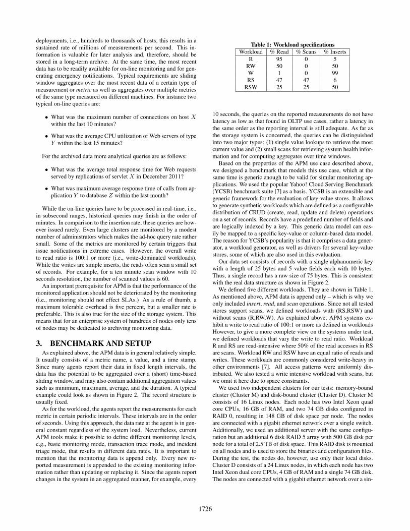
It usually consists of a metric name, a value, and a time stamp.Since many agents report their data in fixed length intervals, thedata has the potential to be aggregated over a (short) time-basedsliding window, and may also contain additional aggregation valuessuch as minimum, maximum, average, and the duration. A typicalexample could look as shown in Figure 2. The record structure isusually fixed.
As for the workload, the agents report the measurements for eachmetric in certain periodic intervals. These intervals are in the orderof seconds. Using this approach, the data rate at the agent is in gen-eral constant regardless of the system load. Nevertheless, currentAPM tools make it possible to define different monitoring levels,e.g., basic monitoring mode, transaction trace mode, and incidenttriage mode, that results in different data rates. It is important tomention that the monitoring data is append only. Every new re-ported measurement is appended to the existing monitoring infor-mation rather than updating or replacing it. Since the agents reportchanges in the system in an aggregated manner, for example, every
Table 1: Workload specificationsWorkload % Read % Scans % Inserts
R 95 0 5RW 50 0 50W 1 0 99RS 47 47 6
RSW 25 25 50
10 seconds, the queries on the reported measurements do not havelatency as low as that found in OLTP use cases, rather a latency inthe same order as the reporting interval is still adequate. As far asthe storage system is concerned, the queries can be distinguishedinto two major types: (1) single value lookups to retrieve the mostcurrent value and (2) small scans for retrieving system health infor-mation and for computing aggregates over time windows.
Based on the properties of the APM use case described above,we designed a benchmark that models this use case, which at thesame time is generic enough to be valid for similar monitoring ap-plications. We used the popular Yahoo! Cloud Serving Benchmark(YCSB) benchmark suite [7] as a basis. YCSB is an extensible andgeneric framework for the evaluation of key-value stores. It allowsto generate synthetic workloads which are defined as a configurabledistribution of CRUD (create, read, update and delete) operationson a set of records. Records have a predefined number of fields andare logically indexed by a key. This generic data model can eas-ily be mapped to a specific key-value or column-based data model.The reason for YCSB’s popularity is that it comprises a data gener-ator, a workload generator, as well as drivers for several key-valuestores, some of which are also used in this evaluation.
Our data set consists of records with a single alphanumeric keywith a length of 25 bytes and 5 value fields each with 10 bytes.Thus, a single record has a raw size of 75 bytes. This is consistentwith the real data structure as shown in Figure 2.
We defined five different workloads. They are shown in Table 1.As mentioned above, APM data is append only – which is why weonly included insert, read, and scan operations. Since not all testedstores support scans, we defined workloads with (RS,RSW) andwithout scans (R,RW,W). As explained above, APM systems ex-hibit a write to read ratio of 100:1 or more as defined in workloadsHowever, to give a more complete view on the systems under test,we defined workloads that vary the write to read ratio. WorkloadR and RS are read-intensive where 50% of the read accesses in RSare scans. Workload RW and RSW have an equal ratio of reads andwrites. These workloads are commonly considered write-heavy inother environments [7]. All access patterns were uniformly dis-tributed. We also tested a write intensive workload with scans, butwe omit it here due to space constraints.
We used two independent clusters for our tests: memory-boundcluster (Cluster M) and disk-bound cluster (Cluster D). Cluster Mconsists of 16 Linux nodes. Each node has two Intel Xeon quadcore CPUs, 16 GB of RAM, and two 74 GB disks configured inRAID 0, resulting in 148 GB of disk space per node. The nodesare connected with a gigabit ethernet network over a single switch.Additionally, we used an additional server with the same configu-ration but an additional 6 disk RAID 5 array with 500 GB disk pernode for a total of 2.5 TB of disk space. This RAID disk is mountedon all nodes and is used to store the binaries and configuration files.During the test, the nodes do, however, use only their local disks.Cluster D consists of a 24 Linux nodes, in which each node has twoIntel Xeon dual core CPUs, 4 GB of RAM and a single 74 GB disk.The nodes are connected with a gigabit ethernet network over a sin-
1726
Metric Name Value Min Max Timestamp DurationHostA/AgentX/ServletB/AverageResponseTime 4 1 6 1332988833 15
Figure 2: Example of an APM measurement
gle switch. We use the Cluster M for memory-bound experimentsand the Cluster D for disk-bound tests.
For Cluster M the size of the data set was set to 10 millionrecords per node resulting 700 MB of raw data per node. The rawdata in this context does not include the keys which increases thetotal data footprint. For Cluster D we tested a single setup with 150million records for a total of 10.5 GB of raw data and thus mak-ing memory-only processing impossible. Each test was run for 600seconds and the reported results are the average of at least 3 inde-pendent executions. We automated the benchmarking process asmuch as possible to be able to experiment with many different set-tings. For each system, we wrote a set of scripts that performed thecomplete benchmark for a given configuration. The scripts installedthe systems from scratch for each workload on the required numberof nodes, thus making sure that there was no interference betweendifferent setups. We made extensive use of the Parallel DistributedShell (pdsh). Many configuration parameters were adapted withinthe scripts using the stream editor sed.
Our workloads were generated using 128 connections per servernode, i.e., 8 connections per core in Cluster M. In Cluster D, wereduced the number of connection to 2 per core to not overloadthe system. The number of connections is equal to the number ofindependently simulated clients for most systems. Thus, we scaledthe number of threads from 128 for one node up to 1536 for 12nodes, all of them working as intensively as possible. To be on thesafe side, we used up to 5 nodes to generate the workload in orderto fully saturate the storage systems. So no client node was runningmore than 307 threads. We set a scan-length of 50 records as wellas fetched all the fields of the record for read operations.
4. BENCHMARKED KEY-VALUE STORESWe benchmarked six different open-source key-value stores. We
chose them to get an overview of the performance impact of dif-ferent storage architectures and design decisions. Our goal wasnot only to get a pure performance comparison but also a broadoverview of available solutions. According to Cartell, new gener-ation data stores can be classified in four main categories [4]. Wechose each two of the following classes according to this classifi-cation:
Key-value stores: Project Voldemort and Redis
Extensible record stores: HBase and Cassandra
Scalable relational stores: MySQL Cluster and VoltDB
Our choice of systems was based on previously reported perfor-mance results, popularity and maturity. Cartell also describes afourth type of store, document stores. However, in our initial re-search we did not find any document store that seemed to matchour requirements and therefore did not include them in the com-parison. In the following, we give a basic overview on the bench-marked systems focusing on the differences. Detailed descriptionscan be found in the referenced literature.
4.1 HBaseHBase [28] is an open source, distributed, column-oriented data-
base system based on Google’s BigTable [5]. HBase is written in
Java, runs on top of Apache Hadoop and Apache ZooKeeper [15]and uses the Hadoop Distributed Filesystem (HDFS) [27] (also anopen source implementation of Google’s file system GFS [13]) inorder to provide fault-tolerance and replication.
Specifically, it provides linear and modular scalability, strictlyconsistent data access, automatic and configurable sharding of data.Tables in HBase can be accessed through an API as well as serve asthe input and output for MapReduce jobs run in Hadoop. In short,applications store data into tables which consist of rows and col-umn families containing columns. Moreover, each row may have adifferent set of columns. Furthermore, all columns are indexed witha user-provided key column and are grouped into column families.Also, all table cells – the intersection of row and column coordi-nates – are versioned and their content is an uninterpreted array ofbytes.
For our benchmarks, we used HBase v0.90.4 running on top ofHadoop v0.20.205.0. The configuration was done using a dedicatednode for the running master processes (NameNode and Secondary-NameNode), therefore for all the benchmarks the specified numberof servers correspond to nodes running slave processes (DataNodesand TaskTrackers) as well as HBase’s region server processes. Weused the already implemented HBase YCSB client, which requiredone table for all the data, storing each field into a different column.
4.2 CassandraApache Cassandra is a second generation distributed key value
store developed at Facebook [19]. It was designed to handle verylarge amounts of data spread out across many commodity serverswhile providing a highly available service without single point offailure allowing replication even across multiple data centers aswell as for choosing between synchronous or asynchronous repli-cation for each update. Also, its elasticity allows read and writethroughput, both increasing linearly as new machines are added,with no downtime or interruption to applications. In short, its ar-chitecture is a mixture of Google’s BigTable [5] and Amazon’s Dy-namo [8]. As in Amazon’s Dynamo, every node in the cluster hasthe same role, so there is no single point of failure as there is inthe case of HBase. The data model provides a structured key-valuestore where columns are added only to specified keys, so differentkeys can have different number of columns in any given family asin HBase. The main differences between Cassandra and HBase arecolumns that can be grouped into column families in a nested wayand consistency requirements that can be specified at query time.Moreover, whereas Cassandra is a write-oriented system, HBasewas designed to get high performance for intensive read workloads.
For our benchmark, we used the recent 1.0.0-rc2 version andused mainly the default configuration. Since we aim for a highwrite throughput and have only small scans, we used the defaultRandomPartitioner that distributes the data across the nodes ran-domly. We used the already implemented Cassandra YCSB clientwhich required to set just one column family to store all the fields,each of them corresponding to a column.
4.3 VoldemortProject Voldemort [29] is a distributed key-value store (devel-
oped by LinkedIn) that provides highly scalable storage system.
1727
With a simpler design compared to a relational database, Volde-mort neither tries to support general relational model nor to guar-antee full ACID properties, instead it simply offers a distributed,fault-tolerant, persistent hash table. In Voldemort, data is automat-ically replicated and partitioned across nodes such that each nodeis responsible for only a subset of data independent from all othernodes. This data model eliminates the central point of failure or theneed for central coordination and allows cluster expansion withoutrebalancing all data, which ultimately allow horizontal scaling ofVoldemort.
Through simple API, data placement and replication can easilybe tuned to accommodate a wide range of application domains. Forinstance, to add persistence, Voldemort can use different storagesystems such as embedded databases (e.g., BerkeleyDB) or stand-alone relational data stores (e.g., MySQL). Other notable featuresof Voldemort are in-memory caching coupled with storage system– so a separate caching tier is no longer required and multi-versiondata model for improved data availability in case of system failure.
In our benchmark, we used version 0.90.1. with the embed-ded BerkeleyDB storage and the already implemented VoldemortYCSB client. Specifically, when configuring the cluster, we settwo partitions per node. In both clusters, we set Voldemort to useabout 75% of the memory whereas the remaining 25% was used forthe embedded BerkeleyDB storage. The data is stored in a singletable where each key is associated with an indexed set of values.
4.4 RedisRedis [24] is an in-memory, key-value data store with the data
durability option. Redis data model supports strings, hashes, lists,sets, and sorted sets. Although Redis is designed for in-memorydata, depending on the use case, data can be (semi-) persisted eitherby taking snapshot of the data and dumping it on disk periodicallyor by maintaining an append-only log of all operations.
Furthermore, Redis can be replicated using a master-slave archi-tecture. Specifically, Redis supports relaxed form of master-slavereplication, in which data from any master can be replicated to anynumber of slaves while a slave may acts as a master to other slavesallowing Redis to model a single-rooted replication tree.
Moreover, Redis replication is non-blocking on both the mas-ter and slave, which means that the master can continue servingqueries when one or more slaves are synchronizing and slaves cananswer queries using the old version of the data during the synchro-nization. This replication model allows for having multiple slavesto answer read-only queries resulting in highly scalable architec-ture.
For our benchmark, we used version 2.4.2. Although a Rediscluster version is expected in the future, at the time of writing thispaper, the cluster version is in an unstable state and we were notable to run a complete test. Therefore, we deployed a single-nodeversion on each of the nodes and used the Jedis6 library to imple-ment a distributed store. We updated the default Redis YCSB clientto use ShardedJedisPool, a class which automatically shards andaccordingly accesses the data in a set of independent Redis servers.This gives considerable advantage to Redis in our benchmark sincethere is no interaction between the Redis instances. For the storageof the data, YCSB uses a hash map as well as a sorted set.
4.5 VoltDBVoltDB [30] is an ACID compliant relational in-memory database
system derived from the research prototype H-Store [17]. It has ashared nothing architecture and is designed to run on a multi-node6Jedis, a Java client for Redis - http://github.com/xetorthio/jedis.
cluster by dividing the database into disjoint partitions by makingeach node the unique owner and responsible for a subset of thepartitions. The unit of transaction is a stored procedure which isJava interspersed with SQL. Forcing stored procedures as the unitof transaction and executing them at the partition containing thenecessary data makes it possible to eliminate round trip messag-ing between SQL statements. The statements are executed seriallyand in a single threaded manner without any locking or latching.The data is in-memory, hence, if it is local to a node a stored pro-cedure can execute without any I/O or network access, providingvery high throughput for transactional workloads. Furthermore,VoltDB supports multi-partition transactions, which require datafrom more than one partition and are therefore more expensive toexecute. Multi-partition transactions can completely be avoided ifthe database is cleanly partitionable.
For our benchmarking we used VoltDB v2.1.3 and the defaultconfiguration. We set 6 sites per host which is the recommenda-tion for our platform. We implemented an YCSB client driver forVoltDB that connects to all servers as suggested in the documenta-tion. We set a single table with 5 columns for each of the fields andthe key as the primary key as well as being the column which allowsVoltDB for computing the partition of the table. This way, as read,write and insert operations are performed for a single key, they areimplemented as single-partition transactions and just the scan op-eration is a multi-partition transaction. Also, we implemented therequired stored procedures for each of the operations as well as theVoltDB YCSB client.
4.6 MySQLMySQL [21] is the world’s most used relational database system
with full SQL support and ACID properties. MySQL supports twomain storage engines: MyISAM (for managing non-transactionaltables) and InnoDB (for providing standard transactional support).In addition, MySQL delivers an in-memory storage abstraction fortemporary or non-persistent data. Furthermore, the MySQL clus-ter edition is a distributed, multi-master database with no singlepoint of failure. In MySQL cluster, tables are automatically shardedacross a pool of low-cost commodity nodes, enabling the databaseto scale horizontally to serve read and write-intensive workloads.
For our benchmarking we used MySQL v5.5.17 and InnoDBas the storage engine. Although MySQL cluster already providesshared-nothing distribution capabilities, instead we spread indepen-dent single-node servers on each node. Thus, we were able to usethe already implemented RDBMS YCSB client which connects tothe databases using JDBC and shards the data using a consistenthashing algorithm. For the storage of the data, a single table with acolumn for each value was used.
5. EXPERIMENTAL RESULTSIn this section, we report the results of our benchmarking efforts.
For each workload, we present the throughput and the latenciesof operations. Since there are huge variations in the latencies, wepresent our results using logarithmic scale. We will first report ourresults and point out significant values, then we will discuss theresults. Most of our experiments were conducted on Cluster Mwhich is the faster system with more main memory. Unless weexplicitly specify the systems were tested on Cluster M.
5.1 Workload RThe first workload was Workload R, which was the most read
intensive with 95% reads and only 5% writes. This kind of work-load is common in many social web information systems wherethe read operations are dominant. As explained above, we used 10
1728
0
20000
40000
60000
80000
100000
120000
140000
160000
180000
2 4 6 8 10 12
Thro
ughput (O
pera
tions/s
ec)
Number of Nodes
CassandraHBase
VoldemortVoltDB
RedisMySQL
Figure 3: Throughput for Workload R
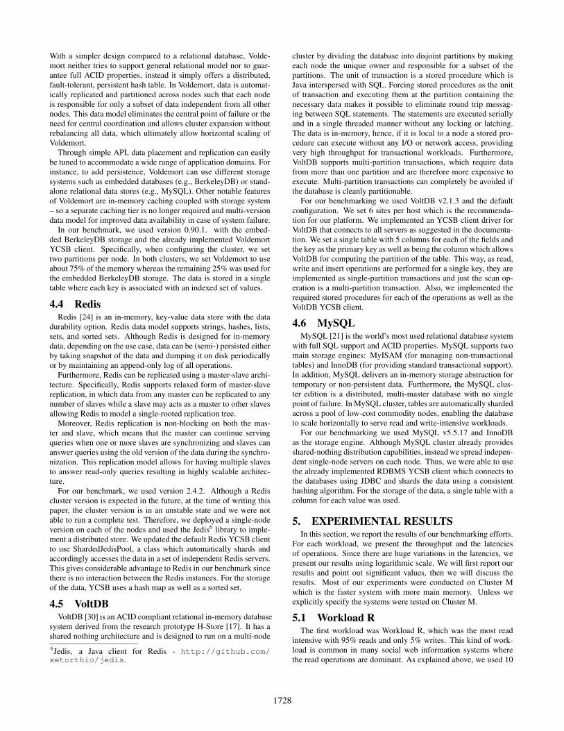
million records per node, thus, scaling the problem size with thecluster size. For each run, we used a freshly installed system andloaded the data. We ran the workload for 10 minutes with max-imum throughput. Figure 3 shows the maximum throughput forworkload R for all six systems.
In the experiment with only one node, Redis has the highestthroughput (more than 50K ops/sec) followed by VoltDB. Thereare no significant differences between the throughput of Cassan-dra and MySQL, which is about half that of Redis (25K ops/sec).Voldemort is 2 times slower than Cassandra (with 12K ops/sec).The slowest system in this test on a single node is HBase with 2.5Koperation per second. However, it is interesting to observe that thethree web data stores that were explicitly built for scalability in webscale – i.e. Cassandra, Voldemort, and HBase – demonstrate a nicelinear behavior in the maximum throughput.
As discussed previously, we were not able to run the cluster ver-sion of Redis, therefore, we used the Jedis library that shards thedata on standalone instances for multiple nodes. In theory, this is abig advantage for Redis, since it does not have to deal with propa-gating data and such. This also puts much more load on the client,therefore, we had to double the number of machines for the YCSBclients for Redis to fully saturate the standalone instances. How-ever, the results do not show the expected scalability. During thetests, we noticed that the data distribution is unbalanced. This ac-tually caused one Redis node to consistently run out of memoryin the 12 node configuration7. For VoltDB, all configurations thatwe tested showed a slow-down for multiple nodes. It seems thatthe synchronous querying in YCSB is not suitable for a distributedVoltDB configuration. For MySQL we used a similar approach asfor Redis. Each MySQL node was independent and the client man-aged the sharding. Interestingly, the YCSB client for MySQL dida much better sharding than the Jedis library, and we observed analmost perfect speed-up from one to two nodes. For higher numberof nodes the increase of the throughput decreased slightly but wascomparable to the throughput of Cassandra.
Workload R was read-intensive and modeled after the require-ments of web information systems. Thus, we expected a low la-tency for read operations at the three web data stores. The averagelatencies for read operations for Workload R can be seen in Figure4. As mentioned before, the latencies are presented in logarithmicscale. For most systems, the read latencies are fairly stable, whilethey differ strongly in the actual value. Again, Cassandra, HBase,and Voldemort illustrate a similar pattern – the latency increasesslightly for two nodes and then stays constant. Project Voldemort
7We tried both supported hashing algorithms in Jedis, Mur-MurHash and MD5, with the same result. The presented resultsare achieved with MurMurHash
0.1
1
10
100
2 4 6 8 10 12
Late
ncy (
ms)
- Logarith
mic
Number of Nodes
CassandraHBase
VoldemortVoltDB
RedisMySQL
Figure 4: Read latency for Workload R
0.01
0.1
1
10
100
2 4 6 8 10 12
Late
ncy (
ms)
- Logarith
mic
Number of Nodes
CassandraHBase
VoldemortVoltDB
RedisMySQL
Figure 5: Write latency for Workload R
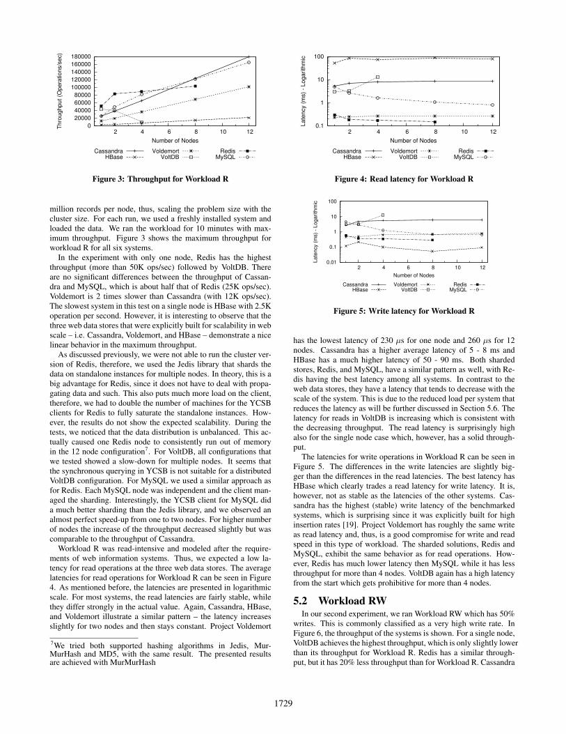
has the lowest latency of 230 µs for one node and 260 µs for 12nodes. Cassandra has a higher average latency of 5 - 8 ms andHBase has a much higher latency of 50 - 90 ms. Both shardedstores, Redis, and MySQL, have a similar pattern as well, with Re-dis having the best latency among all systems. In contrast to theweb data stores, they have a latency that tends to decrease with thescale of the system. This is due to the reduced load per system thatreduces the latency as will be further discussed in Section 5.6. Thelatency for reads in VoltDB is increasing which is consistent withthe decreasing throughput. The read latency is surprisingly highalso for the single node case which, however, has a solid through-put.
The latencies for write operations in Workload R can be seen inFigure 5. The differences in the write latencies are slightly big-ger than the differences in the read latencies. The best latency hasHBase which clearly trades a read latency for write latency. It is,however, not as stable as the latencies of the other systems. Cas-sandra has the highest (stable) write latency of the benchmarkedsystems, which is surprising since it was explicitly built for highinsertion rates [19]. Project Voldemort has roughly the same writeas read latency and, thus, is a good compromise for write and readspeed in this type of workload. The sharded solutions, Redis andMySQL, exhibit the same behavior as for read operations. How-ever, Redis has much lower latency then MySQL while it has lessthroughput for more than 4 nodes. VoltDB again has a high latencyfrom the start which gets prohibitive for more than 4 nodes.
5.2 Workload RWIn our second experiment, we ran Workload RW which has 50%
writes. This is commonly classified as a very high write rate. InFigure 6, the throughput of the systems is shown. For a single node,VoltDB achieves the highest throughput, which is only slightly lowerthan its throughput for Workload R. Redis has a similar through-put, but it has 20% less throughput than for Workload R. Cassandra
1729
0
50000
100000
150000
200000
250000
2 4 6 8 10 12
Thro
ughput (O
ps/s
ec)
Number of Nodes
CassandraHBase
VoldemortVoltDB
RedisMySQL
Figure 6: Throughput for Workload RW
0.1
1
10
100
1000
2 4 6 8 10 12
Late
ncy (
ms)
- Logarith
mic
Number of Nodes
CassandraHBase
VoldemortVoltDB
RedisMySQL
Figure 7: Read latency for Workload RW
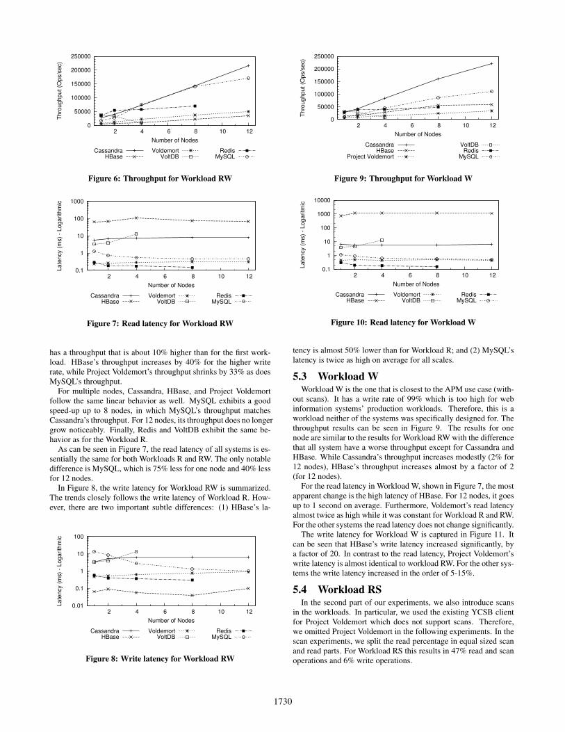
has a throughput that is about 10% higher than for the first work-load. HBase’s throughput increases by 40% for the higher writerate, while Project Voldemort’s throughput shrinks by 33% as doesMySQL’s throughput.
For multiple nodes, Cassandra, HBase, and Project Voldemortfollow the same linear behavior as well. MySQL exhibits a goodspeed-up up to 8 nodes, in which MySQL’s throughput matchesCassandra’s throughput. For 12 nodes, its throughput does no longergrow noticeably. Finally, Redis and VoltDB exhibit the same be-havior as for the Workload R.
As can be seen in Figure 7, the read latency of all systems is es-sentially the same for both Workloads R and RW. The only notabledifference is MySQL, which is 75% less for one node and 40% lessfor 12 nodes.
In Figure 8, the write latency for Workload RW is summarized.The trends closely follows the write latency of Workload R. How-ever, there are two important subtle differences: (1) HBase’s la-
0.01
0.1
1
10
100
2 4 6 8 10 12
Late
ncy (
ms)
- Logarith
mic
Number of Nodes
CassandraHBase
VoldemortVoltDB
RedisMySQL
Figure 8: Write latency for Workload RW
0
50000
100000
150000
200000
250000
2 4 6 8 10 12
Thro
ughput (O
ps/s
ec)
Number of Nodes
CassandraHBase
Project Voldemort
VoltDBRedis
MySQL
Figure 9: Throughput for Workload W
0.1
1
10
100
1000
10000
2 4 6 8 10 12
Late
ncy (
ms)
- Logaritm
ic
Number of Nodes
CassandraHBase
VoldemortVoltDB
RedisMySQL
Figure 10: Read latency for Workload W
tency is almost 50% lower than for Workload R; and (2) MySQL’slatency is twice as high on average for all scales.
5.3 Workload WWorkload W is the one that is closest to the APM use case (with-
out scans). It has a write rate of 99% which is too high for webinformation systems’ production workloads. Therefore, this is aworkload neither of the systems was specifically designed for. Thethroughput results can be seen in Figure 9. The results for onenode are similar to the results for Workload RW with the differencethat all system have a worse throughput except for Cassandra andHBase. While Cassandra’s throughput increases modestly (2% for12 nodes), HBase’s throughput increases almost by a factor of 2(for 12 nodes).
For the read latency in Workload W, shown in Figure 7, the mostapparent change is the high latency of HBase. For 12 nodes, it goesup to 1 second on average. Furthermore, Voldemort’s read latencyalmost twice as high while it was constant for Workload R and RW.For the other systems the read latency does not change significantly.
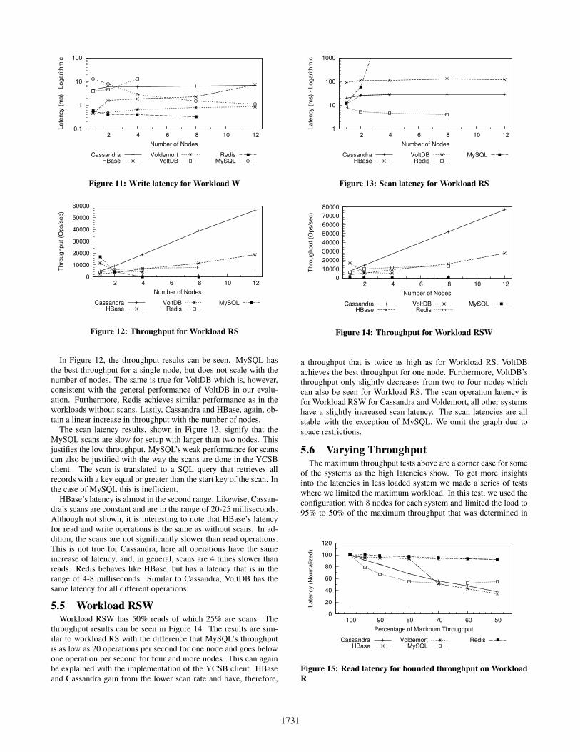
The write latency for Workload W is captured in Figure 11. Itcan be seen that HBase’s write latency increased significantly, bya factor of 20. In contrast to the read latency, Project Voldemort’swrite latency is almost identical to workload RW. For the other sys-tems the write latency increased in the order of 5-15%.
5.4 Workload RSIn the second part of our experiments, we also introduce scans
in the workloads. In particular, we used the existing YCSB clientfor Project Voldemort which does not support scans. Therefore,we omitted Project Voldemort in the following experiments. In thescan experiments, we split the read percentage in equal sized scanand read parts. For Workload RS this results in 47% read and scanoperations and 6% write operations.
1730
0.1
1
10
100
2 4 6 8 10 12
Late
ncy (
ms)
- Logarith
mic
Number of Nodes
CassandraHBase
VoldemortVoltDB
RedisMySQL
Figure 11: Write latency for Workload W
0
10000
20000
30000
40000
50000
60000
2 4 6 8 10 12
Thro
ughput (O
ps/s
ec)
Number of Nodes
CassandraHBase
VoltDBRedis
MySQL
Figure 12: Throughput for Workload RS
In Figure 12, the throughput results can be seen. MySQL hasthe best throughput for a single node, but does not scale with thenumber of nodes. The same is true for VoltDB which is, however,consistent with the general performance of VoltDB in our evalu-ation. Furthermore, Redis achieves similar performance as in theworkloads without scans. Lastly, Cassandra and HBase, again, ob-tain a linear increase in throughput with the number of nodes.
The scan latency results, shown in Figure 13, signify that theMySQL scans are slow for setup with larger than two nodes. Thisjustifies the low throughput. MySQL’s weak performance for scanscan also be justified with the way the scans are done in the YCSBclient. The scan is translated to a SQL query that retrieves allrecords with a key equal or greater than the start key of the scan. Inthe case of MySQL this is inefficient.
HBase’s latency is almost in the second range. Likewise, Cassan-dra’s scans are constant and are in the range of 20-25 milliseconds.Although not shown, it is interesting to note that HBase’s latencyfor read and write operations is the same as without scans. In ad-dition, the scans are not significantly slower than read operations.This is not true for Cassandra, here all operations have the sameincrease of latency, and, in general, scans are 4 times slower thanreads. Redis behaves like HBase, but has a latency that is in therange of 4-8 milliseconds. Similar to Cassandra, VoltDB has thesame latency for all different operations.
5.5 Workload RSWWorkload RSW has 50% reads of which 25% are scans. The
throughput results can be seen in Figure 14. The results are sim-ilar to workload RS with the difference that MySQL’s throughputis as low as 20 operations per second for one node and goes belowone operation per second for four and more nodes. This can againbe explained with the implementation of the YCSB client. HBaseand Cassandra gain from the lower scan rate and have, therefore,
1
10
100
1000
2 4 6 8 10 12
Late
ncy (
ms)
- Logarith
mic
Number of Nodes
CassandraHBase
VoltDBRedis
MySQL
Figure 13: Scan latency for Workload RS
0
10000
20000
30000
40000
50000
60000
70000
80000
2 4 6 8 10 12
Thro
ughput (O
ps/s
ec)
Number of Nodes
CassandraHBase
VoltDBRedis
MySQL
Figure 14: Throughput for Workload RSW
a throughput that is twice as high as for Workload RS. VoltDBachieves the best throughput for one node. Furthermore, VoltDB’sthroughput only slightly decreases from two to four nodes whichcan also be seen for Workload RS. The scan operation latency isfor Workload RSW for Cassandra and Voldemort, all other systemshave a slightly increased scan latency. The scan latencies are allstable with the exception of MySQL. We omit the graph due tospace restrictions.
5.6 Varying ThroughputThe maximum throughput tests above are a corner case for some
of the systems as the high latencies show. To get more insightsinto the latencies in less loaded system we made a series of testswhere we limited the maximum workload. In this test, we used theconfiguration with 8 nodes for each system and limited the load to95% to 50% of the maximum throughput that was determined in
0
20
40
60
80
100
120
50 60 70 80 90 100
Late
ncy (
Norm
aliz
ed)
Percentage of Maximum Throughput
CassandraHBase
VoldemortMySQL
Redis
Figure 15: Read latency for bounded throughput on WorkloadR
1731
0
50
100
150
200
250
50 60 70 80 90 100
Late
ncy (
Norm
aliz
ed)
Percentage of Maximum Throughput
CassandraHBase
VoldemortMySQL
Redis
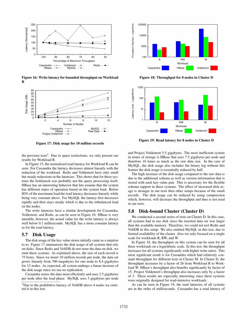
Figure 16: Write latency for bounded throughput on WorkloadR
0 10 20 30 40 50 60 70 80 90
2 4 6 8 10 12
Dis
k U
sage (
GB
)
Number of Nodes
CassandraHBase
Project Voldemort
MySQLRaw Data
Figure 17: Disk usage for 10 million records
the previous tests8. Due to space restrictions, we only present ourresults for Workload R.
In Figure 15, the normalized read latency for Workload R can beseen. For Cassandra the latency decreases almost linearly with thereduction of the workload. Redis and Voldemort have only smallbut steady reductions in the latencies. This shows that for these sys-tems the bottleneck was probably not the query processing itself.HBase has an interesting behavior that lets assume that the systemhas different states of operation based on the system load. Below80% of the maximum load the read latency decreases linearly whilebeing very constant above. For MySQL the latency first decreasesrapidly and then stays steady which is due to the imbalanced loadon the nodes.
The write latencies have a similar development for Cassandra,Voldemort, and Redis, as can be seen in Figure 16. HBase is veryunstable, however, the actual value for the write latency is alwayswell below 0.1 milliseconds. MySQL has a more constant latencyas for the read latency.
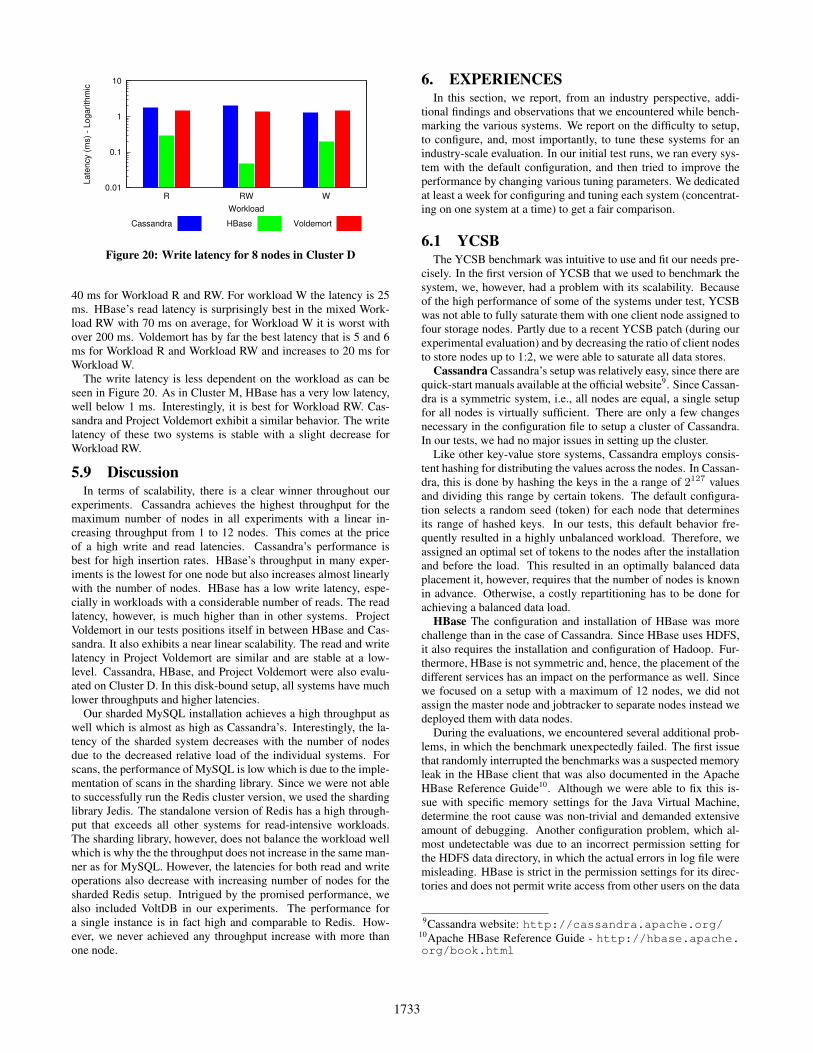
5.7 Disk UsageThe disk usage of the key value stores initially came as a surprise
to us. Figure 17 summarizes the disk usage of all systems that relyon disks. Since Redis and VoltDB do not store the data on disk, weomit these systems. As explained above, the size of each record is75 bytes. Since we insert 10 million records per node, the data setgrows linearly from 700 megabytes for one node to 8.4 gigabytesfor 12 nodes. As expected, all system undergo a linear increase ofthe disk usage since we use no replication.
Cassandra stores the data most efficiently and uses 2.5 gigabytesper node after the load phase. MySQL uses 5 gigabytes per node8Due to the prohibitive latency of VoltDB above 4 nodes we omit-ted it in this test.
100
1000
10000
100000
R RW W
Thro
ughput (O
ps/s
ec)
- Logarith
mic
Workload
Cassandra HBase Voldemort
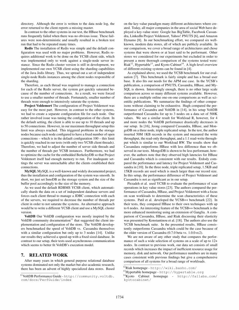
Figure 18: Throughput for 8 nodes in Cluster D
1
10
100
1000
R RW W
Late
ncy (
ms)
- Logarith
mic
Workload
Cassandra HBase Voldemort
Figure 19: Read latency for 8 nodes in Cluster D
and Project Voldemort 5.5 gigabytes. The most inefficient systemin terms of storage is HBase that uses 7.5 gigabytes per node andtherefore 10 times as much as the raw data size. In the case ofMySQL, the disk usage also includes the binary log without thisfeature the disk usage is essentially reduced by half.
The high increase of the disk usage compared to the raw data isdue to the additional schema as well as version information that isstored with each key-value pair. This is necessary for the flexibleschema support in these systems. The effect of increased disk us-age is stronger in our tests then other setups because of the smallrecords. The disk usage can be reduced by using compressionwhich, however, will decrease the throughput and thus is not usedin our tests.
5.8 Disk-bound Cluster (Cluster D)We conducted a second series of tests on Cluster D. In this case,
all systems had to use disk since the inserted data set was largerthan the available memory. Therefore, we could not test Redis andVoltDB in this setup. We also omitted MySQL in this test, due tolimited availability of the cluster. Also we only focused on a singlescale for workloads R, RW, and W.
In Figure 18, the throughput on this system can be seen for allthree workloads on a logarithmic scale. In this test, the throughputincreases for all systems significantly with higher write ratios. Thismost significant result is for Cassandra which had relatively con-stant throughput for different tests in Cluster M. In Cluster D, thethroughput increases by a factor of 26 from Workload R to Work-load W. HBase’s throughput also benefits significantly by factor of15. Project Voldemort’s throughput also increases only by a factorof 3. These results are especially interesting since these systemswere originally designed for read-intensive workloads.
As can be seen in Figure 19, the read latencies of all systemsare in the order of milliseconds. Cassandra has a read latency of
1732
0.01
0.1
1
10
R RW W
Late
ncy (
ms)
- Logarith
mic
Workload
Cassandra HBase Voldemort
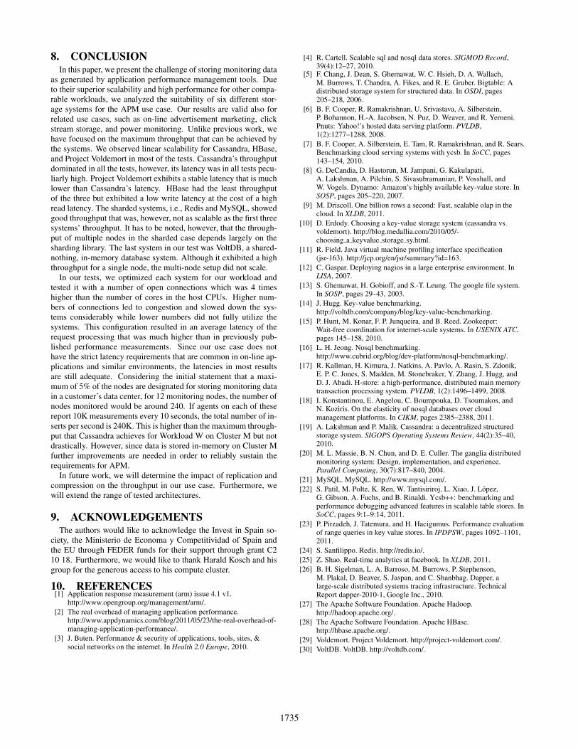
Figure 20: Write latency for 8 nodes in Cluster D
40 ms for Workload R and RW. For workload W the latency is 25ms. HBase’s read latency is surprisingly best in the mixed Work-load RW with 70 ms on average, for Workload W it is worst withover 200 ms. Voldemort has by far the best latency that is 5 and 6ms for Workload R and Workload RW and increases to 20 ms forWorkload W.
The write latency is less dependent on the workload as can beseen in Figure 20. As in Cluster M, HBase has a very low latency,well below 1 ms. Interestingly, it is best for Workload RW. Cas-sandra and Project Voldemort exhibit a similar behavior. The writelatency of these two systems is stable with a slight decrease forWorkload RW.
5.9 DiscussionIn terms of scalability, there is a clear winner throughout our
experiments. Cassandra achieves the highest throughput for themaximum number of nodes in all experiments with a linear in-creasing throughput from 1 to 12 nodes. This comes at the priceof a high write and read latencies. Cassandra’s performance isbest for high insertion rates. HBase’s throughput in many exper-iments is the lowest for one node but also increases almost linearlywith the number of nodes. HBase has a low write latency, espe-cially in workloads with a considerable number of reads. The readlatency, however, is much higher than in other systems. ProjectVoldemort in our tests positions itself in between HBase and Cas-sandra. It also exhibits a near linear scalability. The read and writelatency in Project Voldemort are similar and are stable at a low-level. Cassandra, HBase, and Project Voldemort were also evalu-ated on Cluster D. In this disk-bound setup, all systems have muchlower throughputs and higher latencies.
Our sharded MySQL installation achieves a high throughput aswell which is almost as high as Cassandra’s. Interestingly, the la-tency of the sharded system decreases with the number of nodesdue to the decreased relative load of the individual systems. Forscans, the performance of MySQL is low which is due to the imple-mentation of scans in the sharding library. Since we were not ableto successfully run the Redis cluster version, we used the shardinglibrary Jedis. The standalone version of Redis has a high through-put that exceeds all other systems for read-intensive workloads.The sharding library, however, does not balance the workload wellwhich is why the the throughput does not increase in the same man-ner as for MySQL. However, the latencies for both read and writeoperations also decrease with increasing number of nodes for thesharded Redis setup. Intrigued by the promised performance, wealso included VoltDB in our experiments. The performance fora single instance is in fact high and comparable to Redis. How-ever, we never achieved any throughput increase with more thanone node.
6. EXPERIENCESIn this section, we report, from an industry perspective, addi-
tional findings and observations that we encountered while bench-marking the various systems. We report on the difficulty to setup,to configure, and, most importantly, to tune these systems for anindustry-scale evaluation. In our initial test runs, we ran every sys-tem with the default configuration, and then tried to improve theperformance by changing various tuning parameters. We dedicatedat least a week for configuring and tuning each system (concentrat-ing on one system at a time) to get a fair comparison.
6.1 YCSBThe YCSB benchmark was intuitive to use and fit our needs pre-
cisely. In the first version of YCSB that we used to benchmark thesystem, we, however, had a problem with its scalability. Becauseof the high performance of some of the systems under test, YCSBwas not able to fully saturate them with one client node assigned tofour storage nodes. Partly due to a recent YCSB patch (during ourexperimental evaluation) and by decreasing the ratio of client nodesto store nodes up to 1:2, we were able to saturate all data stores.
Cassandra Cassandra’s setup was relatively easy, since there arequick-start manuals available at the official website9. Since Cassan-dra is a symmetric system, i.e., all nodes are equal, a single setupfor all nodes is virtually sufficient. There are only a few changesnecessary in the configuration file to setup a cluster of Cassandra.In our tests, we had no major issues in setting up the cluster.
Like other key-value store systems, Cassandra employs consis-tent hashing for distributing the values across the nodes. In Cassan-dra, this is done by hashing the keys in the a range of 2127 valuesand dividing this range by certain tokens. The default configura-tion selects a random seed (token) for each node that determinesits range of hashed keys. In our tests, this default behavior fre-quently resulted in a highly unbalanced workload. Therefore, weassigned an optimal set of tokens to the nodes after the installationand before the load. This resulted in an optimally balanced dataplacement it, however, requires that the number of nodes is knownin advance. Otherwise, a costly repartitioning has to be done forachieving a balanced data load.
HBase The configuration and installation of HBase was morechallenge than in the case of Cassandra. Since HBase uses HDFS,it also requires the installation and configuration of Hadoop. Fur-thermore, HBase is not symmetric and, hence, the placement of thedifferent services has an impact on the performance as well. Sincewe focused on a setup with a maximum of 12 nodes, we did notassign the master node and jobtracker to separate nodes instead wedeployed them with data nodes.
During the evaluations, we encountered several additional prob-lems, in which the benchmark unexpectedly failed. The first issuethat randomly interrupted the benchmarks was a suspected memoryleak in the HBase client that was also documented in the ApacheHBase Reference Guide10. Although we were able to fix this is-sue with specific memory settings for the Java Virtual Machine,determine the root cause was non-trivial and demanded extensiveamount of debugging. Another configuration problem, which al-most undetectable was due to an incorrect permission setting forthe HDFS data directory, in which the actual errors in log file weremisleading. HBase is strict in the permission settings for its direc-tories and does not permit write access from other users on the data
9Cassandra website: http://cassandra.apache.org/10Apache HBase Reference Guide - http://hbase.apache.org/book.html
1733
directory. Although the error is written to the data node log, theerror returned to the client reports a missing master.
In contrast to the other systems in our test, the HBase benchmarkruns frequently failed when there was no obvious issue. These fail-ures were non-deterministic and usually resulted in a broken testrun that had to be repeated many times.
Redis The installation of Redis was simple and the default con-figuration was used with no major problems. However, Redis re-quires additional work to be done on the YCSB client side, whichwas implemented only to work against a single-node server in-stance. Since the Redis cluster version is still in development, weimplemented our own YCSB client using the sharding capabilitiesof the Java Jedis library. Thus, we spread out a set of independentsingle-node Redis instances among the client nodes responsible ofthe sharding.
Therefore, as each thread was required to manage a connectionfor each of the Redis server, the system got quickly saturated be-cause of the number of connections. As a result, we were forcedto use a smaller number of threads. Fortunately, smaller number ofthreads were enough to intensively saturate the systems.
Project Voldemort The configuration of Project Voldemort waseasy for the most part. However, in contrast to the other systems,we had to create a separate configuration file for each node. Onerather involved issue was tuning the configuration of the client. Inthe default setting, the client is able to use up to 10 threads and upto 50 connections. However, in our maximum throughput setup thislimit was always reached. This triggered problems in the storagenodes because each node configured to have a fixed number of openconnections – which is in the default configuration 100 – this limitis quickly reached in our tests (with only two YCSB client threads).Therefore, we had to adjust the number of server side threads andthe number of threads per YCSB instances. Furthermore, we hadto optimize the cache for the embedded BerkeleyDB so that ProjectVoldemort itself had enough memory to run. For inadequate set-tings the server was unreachable after the clients established theirconnections.
MySQL MySQL is a well-known and widely documented project,thus the installation and configuration of the system was smooth. Inshort, we just set InnoDB as the storage system and the size of thebuffer pool accordingly to the size of the memory.
As we used the default RDBMS YCSB client, which automati-cally shards the data on a set of independent database servers andforces each client thread to manage a JDBC connection with eachof the servers, we required to decrease the number of threads perclient in order to not saturate the systems. An alternative approachwould be to write a different YCSB client and use a MySQL clusterversion.
VoltDB Our VoltDB configuration was mostly inspired by theVoltDB community documentation11 that suggested the client im-plementation and configuration of the store. The VoltDB develop-ers benchmarked the speed of VoltDB vs. Cassandra themselveswith a similar configuration but only up to 3 nodes [14]. Unlikeour results they achieved a speed-up with a fixed sized database. Incontrast to our setup, their tests used asynchronous communicationwhich seems to better fit VoltDB’s execution model.
7. RELATED WORKAfter many years in which general purpose relational database
systems dominated not only the market but also academic research,there has been an advent of highly specialized data stores. Based
11VoltDB Performance Guide - http://community.voltdb.com/docs/PerfGuide/index
on the key-value paradigm many different architectures where cre-ated. Today, all major companies in the area of social Web have de-ployed a key-value store: Google has BigTable, Facebook Cassan-dra, LinkedIn Project Voldemort, Yahoo! PNUTS [6], and AmazonDynamo [8]. In our benchmarking effort, we compared six well-known, modern data stores, all of which are publicly available. Inour comparison, we cover a broad range of architectures and chosesystems that were shown or at least said to be performant. Otherstores we considered for our experiments but excluded in order topresent a more thorough comparison of the systems tested were:Riak12, Hypertable13, and Kyoto Cabinet14. A high-level overviewof different existing systems can be found in [4].
As explained above, we used the YCSB benchmark for our eval-uation [7]. This benchmark is fairly simple and has a broad userbase. It also fits our needs for the APM use case. In the YCSB’spublication, a comparison of PNUTS, Cassandra, HBase, and My-SQL is shown. Interestingly enough, there is no other large scalecomparison across so many different systems available. However,there are a multiple online one-on-one comparisons as well as sci-entific publications. We summarize the findings of other compar-isons without claiming to be exhaustive. Hugh compared the per-formance of Cassandra and VoltDB in [14], in his setup VoltDBoutperformed Cassandra for up to 3 nodes on a data set of 500Kvalues. We see a similar result for Workload R, however, for 4and more nodes the VoltDB performance drastically decreases inour setup. In [16], Jeong compared Cassandra, HBase, and Mon-goDB on a three node, triple replicated setup. In the test, the authorinserted 50M 1KB records in the system and measured the writethroughput, the read-only throughput, and a 1:1 read-write through-put which is similar to our Workload RW. The results show thatCassandara outperforms HBase with less difference than we ob-served in our tests. MongoDB is shown to be less performant, how-ever, the authors note that they observed high latencies for HBaseand Cassandra which is consistent with our results. Erdody com-pared the performance and latency for Project Voldemort and Cas-sandra in [10]. In the three node, triple replicated setup, 1.5KB and15KB records are used which is much larger than our record size.In this setup, the performance difference of Project Voldemort andCassandra is not as significant as in our setup.
Pirzadeh et al. used YCSB to evaluate the performance of scanoperations in key value stores [23]. The authors compared the per-formance of Cassandra, HBase, and Project Voldemort with a focuson scan workloads to determine the scan characteristics of thesesystems. Patil et al. developed the YCSB++ benchmark [22]. Intheir tests, they compared HBase to their own techniques with upto 6 nodes. An interesting feature of the YCSB++ benchmark is themore enhanced monitoring using an extension of Ganglia. A com-parison of Cassandra, HBase, and Riak discussing their elasticitywas presented by Konstantinou et al. [18]. The authors also use theYCSB benchmark suite. In the presented results, HBase consis-tently outperforms Cassandra which could be the case because ofthe older version of Cassandra (0.7.0 beta vs. 1.0.0-rc2).
We are not aware of any other study that compares the perfor-mance of such a wide selection of systems on a scale of up to 12+nodes. In contrast to previous work, our data set consists of smallrecords which increases the impact of inefficient resource usage formemory, disk and network. Our performance numbers are in manycases consistent with previous findings but give a comprehensivecomparison of all systems for a broad range of workloads.
12Riak homepage - http://wiki.basho.com/13Hypertable homepage - http://hypertable.org14Kyoto Cabinet homepage - http://fallabs.com/kyotocabinet/
1734
8. CONCLUSIONIn this paper, we present the challenge of storing monitoring data
as generated by application performance management tools. Dueto their superior scalability and high performance for other compa-rable workloads, we analyzed the suitability of six different stor-age systems for the APM use case. Our results are valid also forrelated use cases, such as on-line advertisement marketing, clickstream storage, and power monitoring. Unlike previous work, wehave focused on the maximum throughput that can be achieved bythe systems. We observed linear scalability for Cassandra, HBase,and Project Voldemort in most of the tests. Cassandra’s throughputdominated in all the tests, however, its latency was in all tests pecu-liarly high. Project Voldemort exhibits a stable latency that is muchlower than Cassandra’s latency. HBase had the least throughputof the three but exhibited a low write latency at the cost of a highread latency. The sharded systems, i.e., Redis and MySQL, showedgood throughput that was, however, not as scalable as the first threesystems’ throughput. It has to be noted, however, that the through-put of multiple nodes in the sharded case depends largely on thesharding library. The last system in our test was VoltDB, a shared-nothing, in-memory database system. Although it exhibited a highthroughput for a single node, the multi-node setup did not scale.
In our tests, we optimized each system for our workload andtested it with a number of open connections which was 4 timeshigher than the number of cores in the host CPUs. Higher num-bers of connections led to congestion and slowed down the sys-tems considerably while lower numbers did not fully utilize thesystems. This configuration resulted in an average latency of therequest processing that was much higher than in previously pub-lished performance measurements. Since our use case does nothave the strict latency requirements that are common in on-line ap-plications and similar environments, the latencies in most resultsare still adequate. Considering the initial statement that a maxi-mum of 5% of the nodes are designated for storing monitoring datain a customer’s data center, for 12 monitoring nodes, the number ofnodes monitored would be around 240. If agents on each of thesereport 10K measurements every 10 seconds, the total number of in-serts per second is 240K. This is higher than the maximum through-put that Cassandra achieves for Workload W on Cluster M but notdrastically. However, since data is stored in-memory on Cluster Mfurther improvements are needed in order to reliably sustain therequirements for APM.
In future work, we will determine the impact of replication andcompression on the throughput in our use case. Furthermore, wewill extend the range of tested architectures.
9. ACKNOWLEDGEMENTSThe authors would like to acknowledge the Invest in Spain so-
ciety, the Ministerio de Economa y Competitividad of Spain andthe EU through FEDER funds for their support through grant C210 18. Furthermore, we would like to thank Harald Kosch and hisgroup for the generous access to his compute cluster.
10. REFERENCES[1] Application response measurement (arm) issue 4.1 v1.
http://www.opengroup.org/management/arm/.[2] The real overhead of managing application performance.
http://www.appdynamics.com/blog/2011/05/23/the-real-overhead-of-managing-application-performance/.
[3] J. Buten. Performance & security of applications, tools, sites, &social networks on the internet. In Health 2.0 Europe, 2010.
[4] R. Cartell. Scalable sql and nosql data stores. SIGMOD Record,39(4):12–27, 2010.
[5] F. Chang, J. Dean, S. Ghemawat, W. C. Hsieh, D. A. Wallach,M. Burrows, T. Chandra, A. Fikes, and R. E. Gruber. Bigtable: Adistributed storage system for structured data. In OSDI, pages205–218, 2006.
[6] B. F. Cooper, R. Ramakrishnan, U. Srivastava, A. Silberstein,P. Bohannon, H.-A. Jacobsen, N. Puz, D. Weaver, and R. Yerneni.Pnuts: Yahoo!’s hosted data serving platform. PVLDB,1(2):1277–1288, 2008.
[7] B. F. Cooper, A. Silberstein, E. Tam, R. Ramakrishnan, and R. Sears.Benchmarking cloud serving systems with ycsb. In SoCC, pages143–154, 2010.
[8] G. DeCandia, D. Hastorun, M. Jampani, G. Kakulapati,A. Lakshman, A. Pilchin, S. Sivasubramanian, P. Vosshall, andW. Vogels. Dynamo: Amazon’s highly available key-value store. InSOSP, pages 205–220, 2007.
[9] M. Driscoll. One billion rows a second: Fast, scalable olap in thecloud. In XLDB, 2011.
[10] D. Erdody. Choosing a key-value storage system (cassandra vs.voldemort). http://blog.medallia.com/2010/05/-choosing a keyvalue storage sy.html.
[11] R. Field. Java virtual machine profiling interface specification(jsr-163). http://jcp.org/en/jsr/summary?id=163.
[12] C. Gaspar. Deploying nagios in a large enterprise environment. InLISA, 2007.
[13] S. Ghemawat, H. Gobioff, and S.-T. Leung. The google file system.In SOSP, pages 29–43, 2003.
[14] J. Hugg. Key-value benchmarking.http://voltdb.com/company/blog/key-value-benchmarking.
[15] P. Hunt, M. Konar, F. P. Junqueira, and B. Reed. Zookeeper:Wait-free coordination for internet-scale systems. In USENIX ATC,pages 145–158, 2010.
[16] L. H. Jeong. Nosql benchmarking.http://www.cubrid.org/blog/dev-platform/nosql-benchmarking/.
[17] R. Kallman, H. Kimura, J. Natkins, A. Pavlo, A. Rasin, S. Zdonik,E. P. C. Jones, S. Madden, M. Stonebraker, Y. Zhang, J. Hugg, andD. J. Abadi. H-store: a high-performance, distributed main memorytransaction processing system. PVLDB, 1(2):1496–1499, 2008.
[18] I. Konstantinou, E. Angelou, C. Boumpouka, D. Tsoumakos, andN. Koziris. On the elasticity of nosql databases over cloudmanagement platforms. In CIKM, pages 2385–2388, 2011.
[19] A. Lakshman and P. Malik. Cassandra: a decentralized structuredstorage system. SIGOPS Operating Systems Review, 44(2):35–40,2010.
[20] M. L. Massie, B. N. Chun, and D. E. Culler. The ganglia distributedmonitoring system: Design, implementation, and experience.Parallel Computing, 30(7):817–840, 2004.
[21] MySQL. MySQL. http://www.mysql.com/.[22] S. Patil, M. Polte, K. Ren, W. Tantisiriroj, L. Xiao, J. Lopez,
G. Gibson, A. Fuchs, and B. Rinaldi. Ycsb++: benchmarking andperformance debugging advanced features in scalable table stores. InSoCC, pages 9:1–9:14, 2011.
[23] P. Pirzadeh, J. Tatemura, and H. Hacigumus. Performance evaluationof range queries in key value stores. In IPDPSW, pages 1092–1101,2011.
[24] S. Sanfilippo. Redis. http://redis.io/.[25] Z. Shao. Real-time analytics at facebook. In XLDB, 2011.[26] B. H. Sigelman, L. A. Barroso, M. Burrows, P. Stephenson,
M. Plakal, D. Beaver, S. Jaspan, and C. Shanbhag. Dapper, alarge-scale distributed systems tracing infrastructure. TechnicalReport dapper-2010-1, Google Inc., 2010.
[27] The Apache Software Foundation. Apache Hadoop.http://hadoop.apache.org/.
[28] The Apache Software Foundation. Apache HBase.http://hbase.apache.org/.
[29] Voldemort. Project Voldemort. http://project-voldemort.com/.[30] VoltDB. VoltDB. http://voltdb.com/.
1735