solving connectivity problems via basic linear algebra
TRANSCRIPT
Solving connectivity problems via basic LinearAlgebra
Samir DattaChennai Mathematical Institute
Includes joint work with
Raghav Kulkarni Anish Mukherjee Thomas Schwentick
Thomas Zeume
NMI Workshop on ComplexityIIT Gandhinagar
November 6, 2016

Outline
1 Part I: Disjoint Paths
2 Part II: Dynamic Reachability
3 Conclusion
Two fundamental problems
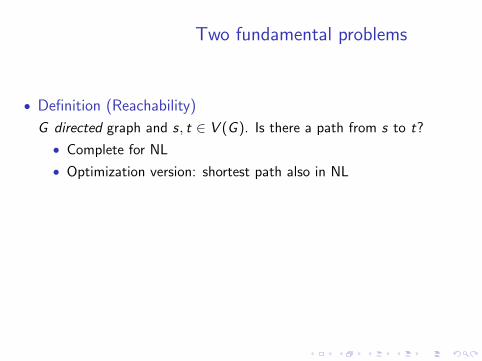
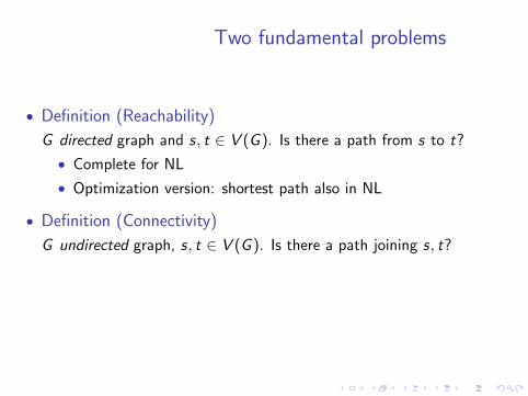
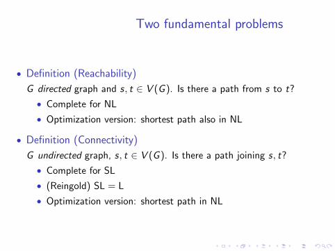
• Definition (Reachability)
G directed graph and s, t ∈ V (G ). Is there a path from s to t?
• Complete for NL
• Optimization version: shortest path also in NL
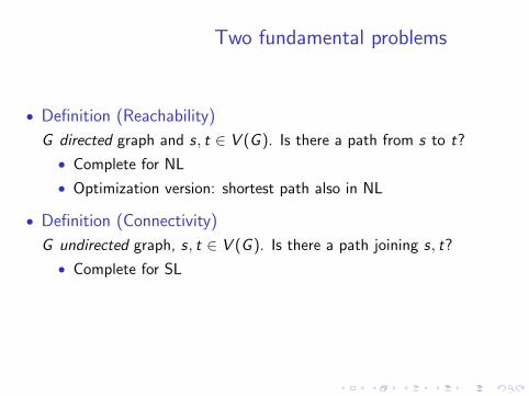
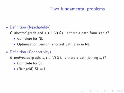
• Definition (Connectivity)
G undirected graph, s, t ∈ V (G ). Is there a path joining s, t?
• Complete for SL
• (Reingold) SL = L
• Optimization version: shortest path in NL
Two fundamental problems
• Definition (Reachability)
G directed graph and s, t ∈ V (G ). Is there a path from s to t?
• Complete for NL
• Optimization version: shortest path also in NL
• Definition (Connectivity)
G undirected graph, s, t ∈ V (G ). Is there a path joining s, t?
• Complete for SL
• (Reingold) SL = L
• Optimization version: shortest path in NL
Disjoint Path Problem
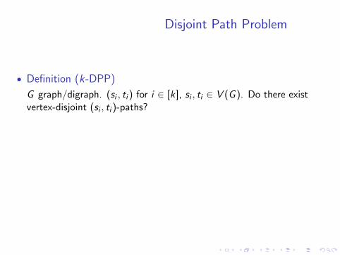
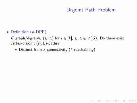
• Definition (k-DPP)
G graph/digraph. (si , ti ) for i ∈ [k], si , ti ∈ V (G ). Do there existvertex-disjoint (si , ti )-paths?
• Distinct from k-connectivity (k-reachability)
• NP-complete for directed graphs for k = 2
• NP-complete for undirected graphs when k part of input.
• (Robertson-Seymour) Cubic time (fixed k) in undirectedgraphs.
• Special cases: Planar graphs/DAGs well studied.
Disjoint Path Problem
• Definition (k-DPP)
G graph/digraph. (si , ti ) for i ∈ [k], si , ti ∈ V (G ). Do there existvertex-disjoint (si , ti )-paths?
• Distinct from k-connectivity (k-reachability)
• NP-complete for directed graphs for k = 2
• NP-complete for undirected graphs when k part of input.
• (Robertson-Seymour) Cubic time (fixed k) in undirectedgraphs.
• Special cases: Planar graphs/DAGs well studied.
One-face Min-sum Disjoint Path Problem
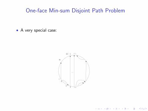
• A very special case:
• k-DPP instance with undirected planar graph, and• All terminals on single face, and• Want solution with minimum total length of paths.
12
4
2k
2k − 1
3
One-face Min-sum Disjoint Path Problem
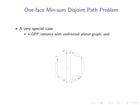
• A very special case:• k-DPP instance with undirected planar graph, and
• All terminals on single face, and• Want solution with minimum total length of paths.
12
4
2k
2k − 1
3
One-face Min-sum Disjoint Path Problem
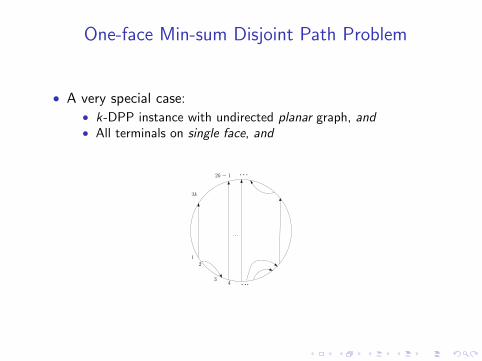
• A very special case:• k-DPP instance with undirected planar graph, and• All terminals on single face, and
• Want solution with minimum total length of paths.
12
4
2k
2k − 1
3
One-face Min-sum Disjoint Path Problem
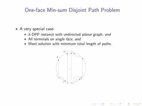
• A very special case:• k-DPP instance with undirected planar graph, and• All terminals on single face, and• Want solution with minimum total length of paths.
12
4
2k
2k − 1
3
One-face Min-sum Disjoint Path Problem:Motivation
• Directed general case remains NP-hard in the plane thoughfixed parameter tractable in k .
• NP-hardness in undirected case: open for k > 2.
• (Bjorklund-Husfeldt’14) Randomized polynomial timealgorithm in undirected case for 2-DPP.
One-face Min-sum Disjoint Path Problem:Motivation
• Directed general case remains NP-hard in the plane thoughfixed parameter tractable in k .
• NP-hardness in undirected case: open for k > 2.
• (Bjorklund-Husfeldt’14) Randomized polynomial timealgorithm in undirected case for 2-DPP.
One-face Min-sum Disjoint Path Problem:Motivation
• Directed general case remains NP-hard in the plane thoughfixed parameter tractable in k .
• NP-hardness in undirected case: open for k > 2.
• (Bjorklund-Husfeldt’14) Randomized polynomial timealgorithm in undirected case for 2-DPP.
One-face Min-sum Disjoint Path Problem:Motivation
• (de Verdiere-Schrijver’08) Two-face case with sources andsinks on two different faces in time O(kn log n).
• (Kobayashi-Sommer’10) One-face min-sum 3-DPP inpolynomial time
• (Borradaile-Nayyeri-Zafarani’15) One-face min-sum k-DPP in“serial” configuration in polynomial time (in n as well as k).
One-face min-sum Disjoint Path Problem:Our Results
Theorem
• The count of One-face min-sum k-DPP solutions can bereduced to O(4k) determinant computations.
• Finding a witness to the problem can be randomly reduced toO(4k) determinant computations.
• Can also do the above sequentially in deterministic O(4knω)time (ω matrix multiplication constant).
Determinant
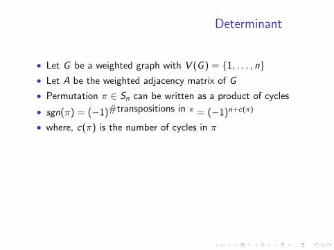
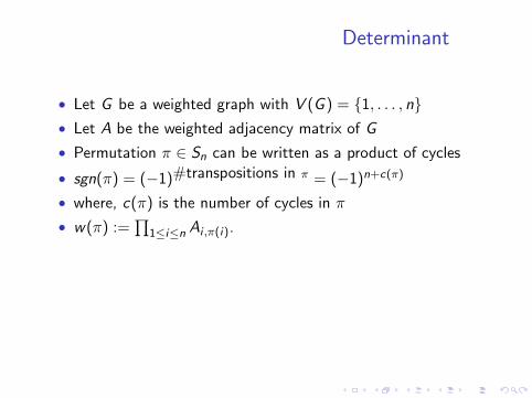
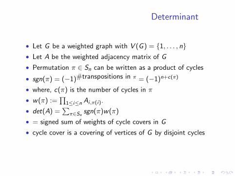
• Let G be a weighted graph with V (G ) = {1, . . . , n}
• Let A be the weighted adjacency matrix of G
• Permutation π ∈ Sn can be written as a product of cycles
• sgn(π) = (−1)#transpositions in π = (−1)n+c(π)
• where, c(π) is the number of cycles in π
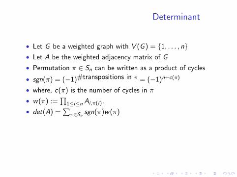
• w(π) :=∏
1≤i≤n Ai ,π(i).
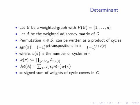
• det(A) =∑
π∈Sn sgn(π)w(π)
• = signed sum of weights of cycle covers in G
• cycle cover is a covering of vertices of G by disjoint cycles
• (cycles include self loops)
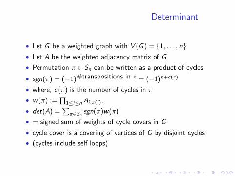
Determinant
• Let G be a weighted graph with V (G ) = {1, . . . , n}• Let A be the weighted adjacency matrix of G
• Permutation π ∈ Sn can be written as a product of cycles
• sgn(π) = (−1)#transpositions in π = (−1)n+c(π)
• where, c(π) is the number of cycles in π
• w(π) :=∏
1≤i≤n Ai ,π(i).
• det(A) =∑
π∈Sn sgn(π)w(π)
• = signed sum of weights of cycle covers in G
• cycle cover is a covering of vertices of G by disjoint cycles
• (cycles include self loops)
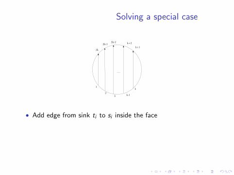
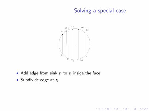
Solving a special case
1
23 k-1
k
k+1
k+22k-22k-1
2k
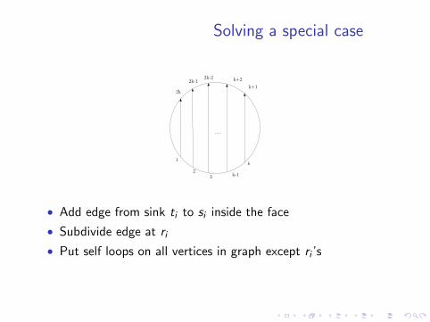
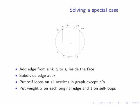
• Add edge from sink ti to si inside the face
• Subdivide edge at ri
• Put self loops on all vertices in graph except ri ’s
• Put weight x on each original edge and 1 on self-loops
Solving a special case
1
23 k-1
k
k+1
k+22k-22k-1
2k
• Add edge from sink ti to si inside the face
• Subdivide edge at ri
• Put self loops on all vertices in graph except ri ’s
• Put weight x on each original edge and 1 on self-loops
Solving a special case
1
23 k-1
k
k+1
k+22k-22k-1
2k
• Add edge from sink ti to si inside the face
• Subdivide edge at ri
• Put self loops on all vertices in graph except ri ’s
• Put weight x on each original edge and 1 on self-loops
Solving a special case
1
23 k-1
k
k+1
k+22k-22k-1
2k
• Add edge from sink ti to si inside the face
• Subdivide edge at ri
• Put self loops on all vertices in graph except ri ’s
• Put weight x on each original edge and 1 on self-loops
Solving a special case
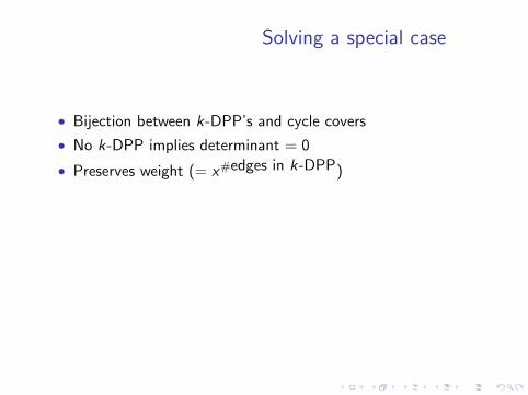
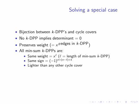
• Bijection between k-DPP’s and cycle covers
• No k-DPP implies determinant = 0
• Preserves weight (= x#edges in k-DPP)
• All min-sum k-DPPs are:
• Same weight = x` (` = length of min-sum k-DPP)• Same sign = (−1)n+(n−`)+k
• Lighter than any other cycle cover
• coefficient of smallest degree term counts #-min-sum k-DPPs
• As easy as determinant
Solving a special case
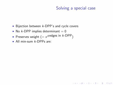
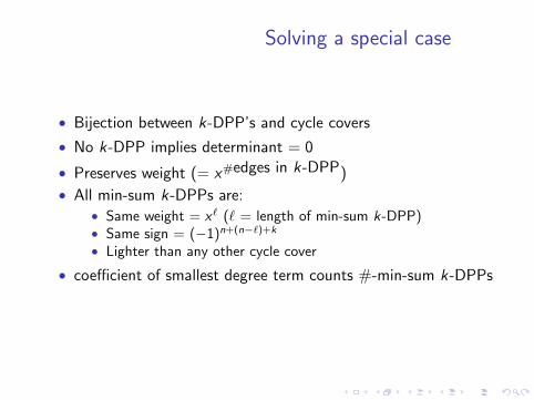
• Bijection between k-DPP’s and cycle covers
• No k-DPP implies determinant = 0
• Preserves weight (= x#edges in k-DPP)
• All min-sum k-DPPs are:
• Same weight = x` (` = length of min-sum k-DPP)• Same sign = (−1)n+(n−`)+k
• Lighter than any other cycle cover
• coefficient of smallest degree term counts #-min-sum k-DPPs
• As easy as determinant
Solving a special case
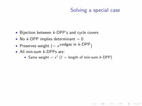
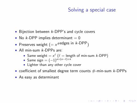
• Bijection between k-DPP’s and cycle covers
• No k-DPP implies determinant = 0
• Preserves weight (= x#edges in k-DPP)
• All min-sum k-DPPs are:
• Same weight = x` (` = length of min-sum k-DPP)• Same sign = (−1)n+(n−`)+k
• Lighter than any other cycle cover
• coefficient of smallest degree term counts #-min-sum k-DPPs
• As easy as determinant
Solving a special case
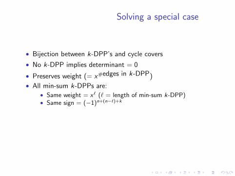
• Bijection between k-DPP’s and cycle covers
• No k-DPP implies determinant = 0
• Preserves weight (= x#edges in k-DPP)
• All min-sum k-DPPs are:• Same weight = x` (` = length of min-sum k-DPP)
• Same sign = (−1)n+(n−`)+k
• Lighter than any other cycle cover
• coefficient of smallest degree term counts #-min-sum k-DPPs
• As easy as determinant
Solving a special case
• Bijection between k-DPP’s and cycle covers
• No k-DPP implies determinant = 0
• Preserves weight (= x#edges in k-DPP)
• All min-sum k-DPPs are:• Same weight = x` (` = length of min-sum k-DPP)• Same sign = (−1)n+(n−`)+k
• Lighter than any other cycle cover
• coefficient of smallest degree term counts #-min-sum k-DPPs
• As easy as determinant
Solving a special case
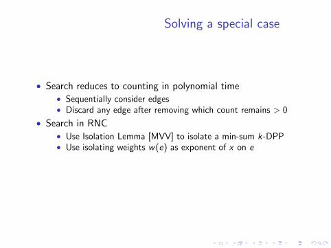
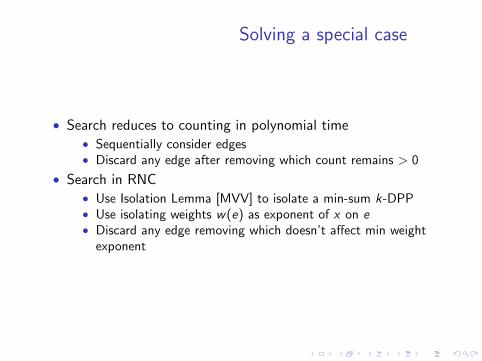
• Search reduces to counting in polynomial time
• Sequentially consider edges• Discard any edge after removing which count remains > 0
• Search in RNC
• Use Isolation Lemma [MVV] to isolate a min-sum k-DPP• Use isolating weights w(e) as exponent of x on e• Discard any edge removing which doesn’t affect min weight
exponent
Solving a special case
• Search reduces to counting in polynomial time• Sequentially consider edges
• Discard any edge after removing which count remains > 0
• Search in RNC
• Use Isolation Lemma [MVV] to isolate a min-sum k-DPP• Use isolating weights w(e) as exponent of x on e• Discard any edge removing which doesn’t affect min weight
exponent
Solving a special case
• Search reduces to counting in polynomial time• Sequentially consider edges• Discard any edge after removing which count remains > 0
• Search in RNC• Use Isolation Lemma [MVV] to isolate a min-sum k-DPP
• Use isolating weights w(e) as exponent of x on e• Discard any edge removing which doesn’t affect min weight
exponent
Solving a special case
• Search reduces to counting in polynomial time• Sequentially consider edges• Discard any edge after removing which count remains > 0
• Search in RNC• Use Isolation Lemma [MVV] to isolate a min-sum k-DPP• Use isolating weights w(e) as exponent of x on e
• Discard any edge removing which doesn’t affect min weightexponent
Solving a special case
• Search reduces to counting in polynomial time• Sequentially consider edges• Discard any edge after removing which count remains > 0
• Search in RNC• Use Isolation Lemma [MVV] to isolate a min-sum k-DPP• Use isolating weights w(e) as exponent of x on e• Discard any edge removing which doesn’t affect min weight
exponent
Issues with general case
1
2 3
4
5
67
8
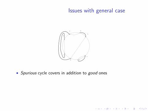
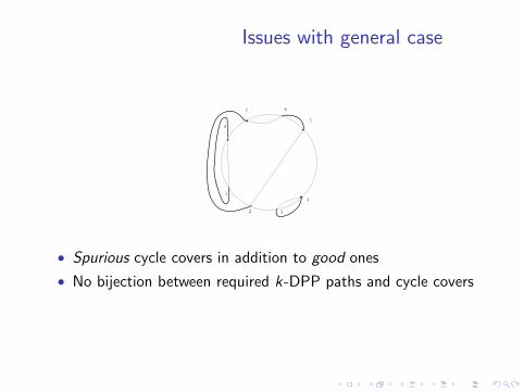
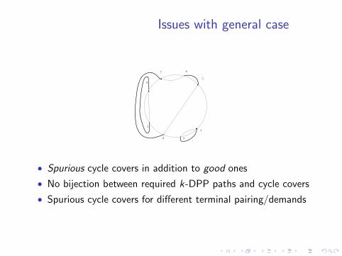
• Spurious cycle covers in addition to good ones
• No bijection between required k-DPP paths and cycle covers
• Spurious cycle covers for different terminal pairing/demands
Issues with general case
1
2 3
4
5
67
8
• Spurious cycle covers in addition to good ones
• No bijection between required k-DPP paths and cycle covers
• Spurious cycle covers for different terminal pairing/demands
Issues with general case
1
2 3
4
5
67
8
• Spurious cycle covers in addition to good ones
• No bijection between required k-DPP paths and cycle covers
• Spurious cycle covers for different terminal pairing/demands

Fixing issues with general case
1
2 3
4
5
67
8
1
2 3
4
5
67
8
1
2 3
4
5
67
8
• Spurious cycle covers canceled by cycle covers with newdemands
• Further spurious cycles - canceled by another demand set -etc.
• Need to prove that process converges

Fixing issues with general case
1
2 3
4
5
67
8
1
2 3
4
5
67
8
1
2 3
4
5
67
8
• Spurious cycle covers canceled by cycle covers with newdemands
• Further spurious cycles - canceled by another demand set -etc.
• Need to prove that process converges

Fixing issues with general case
1
2 3
4
5
67
8
1
2 3
4
5
67
8
1
2 3
4
5
67
8
• Spurious cycle covers canceled by cycle covers with newdemands
• Further spurious cycles - canceled by another demand set -etc.
• Need to prove that process converges
Fixing issues with general case
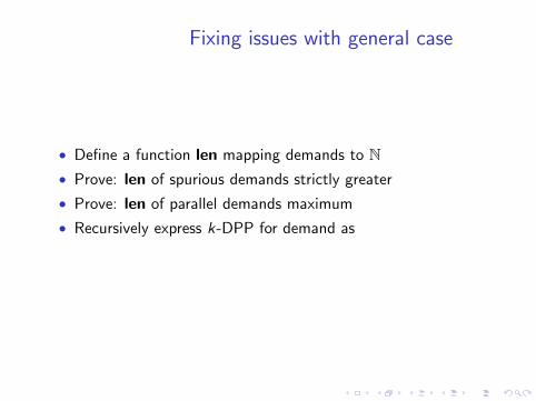
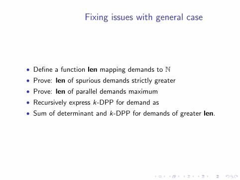
• Define a function len mapping demands to N
• Prove: len of spurious demands strictly greater
• Prove: len of parallel demands maximum
• Recursively express k-DPP for demand as
• Sum of determinant and k-DPP for demands of greater len.
Fixing issues with general case
• Define a function len mapping demands to N• Prove: len of spurious demands strictly greater
• Prove: len of parallel demands maximum
• Recursively express k-DPP for demand as
• Sum of determinant and k-DPP for demands of greater len.
Fixing issues with general case
• Define a function len mapping demands to N• Prove: len of spurious demands strictly greater
• Prove: len of parallel demands maximum
• Recursively express k-DPP for demand as
• Sum of determinant and k-DPP for demands of greater len.
Fixing issues with general case
• Define a function len mapping demands to N• Prove: len of spurious demands strictly greater
• Prove: len of parallel demands maximum
• Recursively express k-DPP for demand as
• Sum of determinant and k-DPP for demands of greater len.
Fixing issues with general case
• Define a function len mapping demands to N• Prove: len of spurious demands strictly greater
• Prove: len of parallel demands maximum
• Recursively express k-DPP for demand as
• Sum of determinant and k-DPP for demands of greater len.

Outline
1 Part I: Disjoint Paths
2 Part II: Dynamic Reachability
3 Conclusion

Two fundamental problems
• Definition (Reachability)
G directed graph and s, t ∈ V (G ). Is there a path from s to t?
• Complete for NL
• Optimization version: shortest path also in NL
• Definition (Connectivity)
G undirected graph, s, t ∈ V (G ). Is there a path joining s, t?
• Complete for SL
• (Reingold) SL = L
• Optimization version: shortest path in NL
Dynamic Complexity
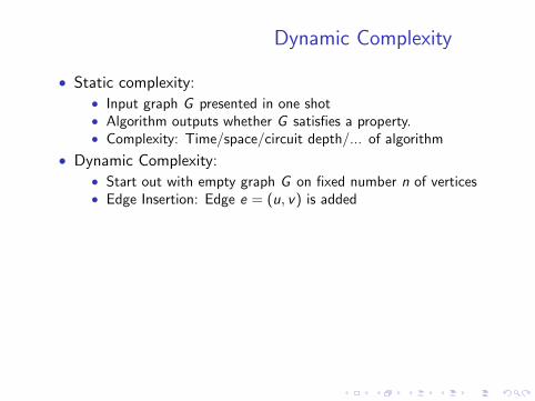
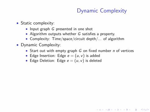
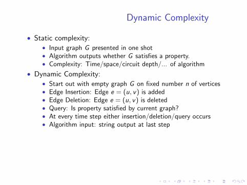
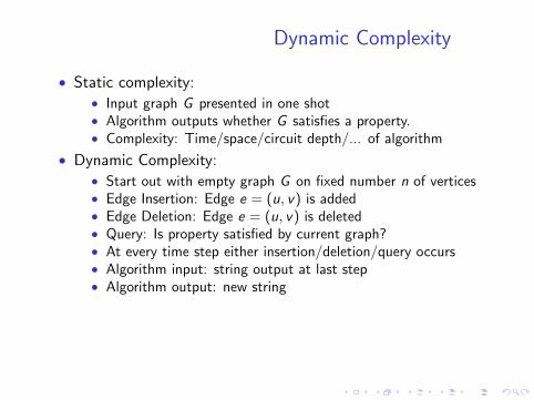
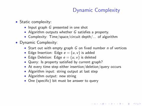
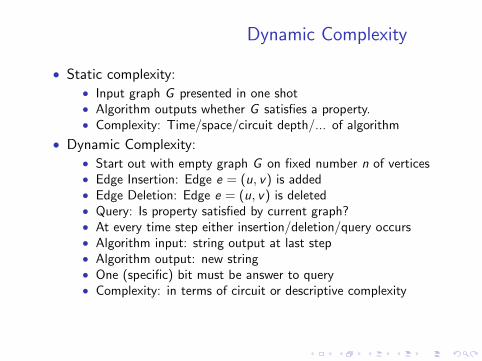
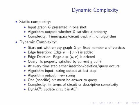
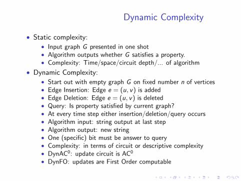
• Static complexity:
• Input graph G presented in one shot• Algorithm outputs whether G satisfies a property.• Complexity: Time/space/circuit depth/... of algorithm
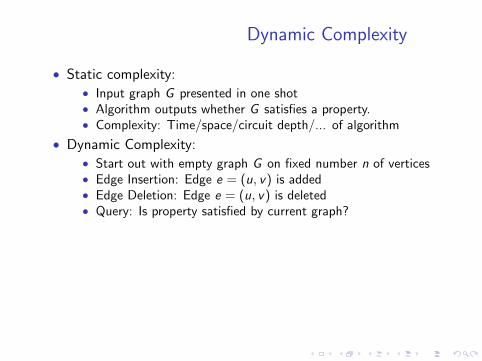
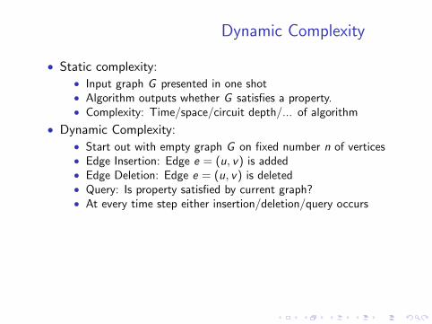
• Dynamic Complexity:
• Start out with empty graph G on fixed number n of vertices• Edge Insertion: Edge e = (u, v) is added• Edge Deletion: Edge e = (u, v) is deleted• Query: Is property satisfied by current graph?• At every time step either insertion/deletion/query occurs• Algorithm input: string output at last step• Algorithm output: new string• One (specific) bit must be answer to query• Complexity: in terms of circuit or descriptive complexity• DynAC0: update circuit is AC0
• DynFO: updates are First Order computable
Dynamic Complexity
• Static complexity:• Input graph G presented in one shot
• Algorithm outputs whether G satisfies a property.• Complexity: Time/space/circuit depth/... of algorithm
• Dynamic Complexity:
• Start out with empty graph G on fixed number n of vertices• Edge Insertion: Edge e = (u, v) is added• Edge Deletion: Edge e = (u, v) is deleted• Query: Is property satisfied by current graph?• At every time step either insertion/deletion/query occurs• Algorithm input: string output at last step• Algorithm output: new string• One (specific) bit must be answer to query• Complexity: in terms of circuit or descriptive complexity• DynAC0: update circuit is AC0
• DynFO: updates are First Order computable
Dynamic Complexity
• Static complexity:• Input graph G presented in one shot• Algorithm outputs whether G satisfies a property.
• Complexity: Time/space/circuit depth/... of algorithm
• Dynamic Complexity:
• Start out with empty graph G on fixed number n of vertices• Edge Insertion: Edge e = (u, v) is added• Edge Deletion: Edge e = (u, v) is deleted• Query: Is property satisfied by current graph?• At every time step either insertion/deletion/query occurs• Algorithm input: string output at last step• Algorithm output: new string• One (specific) bit must be answer to query• Complexity: in terms of circuit or descriptive complexity• DynAC0: update circuit is AC0
• DynFO: updates are First Order computable
Dynamic Complexity
• Static complexity:• Input graph G presented in one shot• Algorithm outputs whether G satisfies a property.• Complexity: Time/space/circuit depth/... of algorithm
• Dynamic Complexity:• Start out with empty graph G on fixed number n of vertices
• Edge Insertion: Edge e = (u, v) is added• Edge Deletion: Edge e = (u, v) is deleted• Query: Is property satisfied by current graph?• At every time step either insertion/deletion/query occurs• Algorithm input: string output at last step• Algorithm output: new string• One (specific) bit must be answer to query• Complexity: in terms of circuit or descriptive complexity• DynAC0: update circuit is AC0
• DynFO: updates are First Order computable
Dynamic Complexity
• Static complexity:• Input graph G presented in one shot• Algorithm outputs whether G satisfies a property.• Complexity: Time/space/circuit depth/... of algorithm
• Dynamic Complexity:• Start out with empty graph G on fixed number n of vertices• Edge Insertion: Edge e = (u, v) is added
• Edge Deletion: Edge e = (u, v) is deleted• Query: Is property satisfied by current graph?• At every time step either insertion/deletion/query occurs• Algorithm input: string output at last step• Algorithm output: new string• One (specific) bit must be answer to query• Complexity: in terms of circuit or descriptive complexity• DynAC0: update circuit is AC0
• DynFO: updates are First Order computable
Dynamic Complexity
• Static complexity:• Input graph G presented in one shot• Algorithm outputs whether G satisfies a property.• Complexity: Time/space/circuit depth/... of algorithm
• Dynamic Complexity:• Start out with empty graph G on fixed number n of vertices• Edge Insertion: Edge e = (u, v) is added• Edge Deletion: Edge e = (u, v) is deleted
• Query: Is property satisfied by current graph?• At every time step either insertion/deletion/query occurs• Algorithm input: string output at last step• Algorithm output: new string• One (specific) bit must be answer to query• Complexity: in terms of circuit or descriptive complexity• DynAC0: update circuit is AC0
• DynFO: updates are First Order computable
Dynamic Complexity
• Static complexity:• Input graph G presented in one shot• Algorithm outputs whether G satisfies a property.• Complexity: Time/space/circuit depth/... of algorithm
• Dynamic Complexity:• Start out with empty graph G on fixed number n of vertices• Edge Insertion: Edge e = (u, v) is added• Edge Deletion: Edge e = (u, v) is deleted• Query: Is property satisfied by current graph?
• At every time step either insertion/deletion/query occurs• Algorithm input: string output at last step• Algorithm output: new string• One (specific) bit must be answer to query• Complexity: in terms of circuit or descriptive complexity• DynAC0: update circuit is AC0
• DynFO: updates are First Order computable
Dynamic Complexity
• Static complexity:• Input graph G presented in one shot• Algorithm outputs whether G satisfies a property.• Complexity: Time/space/circuit depth/... of algorithm
• Dynamic Complexity:• Start out with empty graph G on fixed number n of vertices• Edge Insertion: Edge e = (u, v) is added• Edge Deletion: Edge e = (u, v) is deleted• Query: Is property satisfied by current graph?• At every time step either insertion/deletion/query occurs
• Algorithm input: string output at last step• Algorithm output: new string• One (specific) bit must be answer to query• Complexity: in terms of circuit or descriptive complexity• DynAC0: update circuit is AC0
• DynFO: updates are First Order computable
Dynamic Complexity
• Static complexity:• Input graph G presented in one shot• Algorithm outputs whether G satisfies a property.• Complexity: Time/space/circuit depth/... of algorithm
• Dynamic Complexity:• Start out with empty graph G on fixed number n of vertices• Edge Insertion: Edge e = (u, v) is added• Edge Deletion: Edge e = (u, v) is deleted• Query: Is property satisfied by current graph?• At every time step either insertion/deletion/query occurs• Algorithm input: string output at last step
• Algorithm output: new string• One (specific) bit must be answer to query• Complexity: in terms of circuit or descriptive complexity• DynAC0: update circuit is AC0
• DynFO: updates are First Order computable
Dynamic Complexity
• Static complexity:• Input graph G presented in one shot• Algorithm outputs whether G satisfies a property.• Complexity: Time/space/circuit depth/... of algorithm
• Dynamic Complexity:• Start out with empty graph G on fixed number n of vertices• Edge Insertion: Edge e = (u, v) is added• Edge Deletion: Edge e = (u, v) is deleted• Query: Is property satisfied by current graph?• At every time step either insertion/deletion/query occurs• Algorithm input: string output at last step• Algorithm output: new string
• One (specific) bit must be answer to query• Complexity: in terms of circuit or descriptive complexity• DynAC0: update circuit is AC0
• DynFO: updates are First Order computable
Dynamic Complexity
• Static complexity:• Input graph G presented in one shot• Algorithm outputs whether G satisfies a property.• Complexity: Time/space/circuit depth/... of algorithm
• Dynamic Complexity:• Start out with empty graph G on fixed number n of vertices• Edge Insertion: Edge e = (u, v) is added• Edge Deletion: Edge e = (u, v) is deleted• Query: Is property satisfied by current graph?• At every time step either insertion/deletion/query occurs• Algorithm input: string output at last step• Algorithm output: new string• One (specific) bit must be answer to query
• Complexity: in terms of circuit or descriptive complexity• DynAC0: update circuit is AC0
• DynFO: updates are First Order computable
Dynamic Complexity
• Static complexity:• Input graph G presented in one shot• Algorithm outputs whether G satisfies a property.• Complexity: Time/space/circuit depth/... of algorithm
• Dynamic Complexity:• Start out with empty graph G on fixed number n of vertices• Edge Insertion: Edge e = (u, v) is added• Edge Deletion: Edge e = (u, v) is deleted• Query: Is property satisfied by current graph?• At every time step either insertion/deletion/query occurs• Algorithm input: string output at last step• Algorithm output: new string• One (specific) bit must be answer to query• Complexity: in terms of circuit or descriptive complexity
• DynAC0: update circuit is AC0
• DynFO: updates are First Order computable
Dynamic Complexity
• Static complexity:• Input graph G presented in one shot• Algorithm outputs whether G satisfies a property.• Complexity: Time/space/circuit depth/... of algorithm
• Dynamic Complexity:• Start out with empty graph G on fixed number n of vertices• Edge Insertion: Edge e = (u, v) is added• Edge Deletion: Edge e = (u, v) is deleted• Query: Is property satisfied by current graph?• At every time step either insertion/deletion/query occurs• Algorithm input: string output at last step• Algorithm output: new string• One (specific) bit must be answer to query• Complexity: in terms of circuit or descriptive complexity• DynAC0: update circuit is AC0
• DynFO: updates are First Order computable
Dynamic Reachability
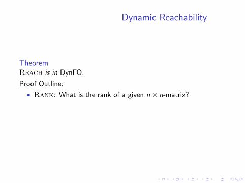
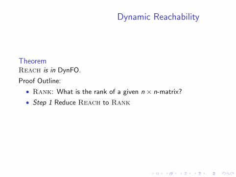
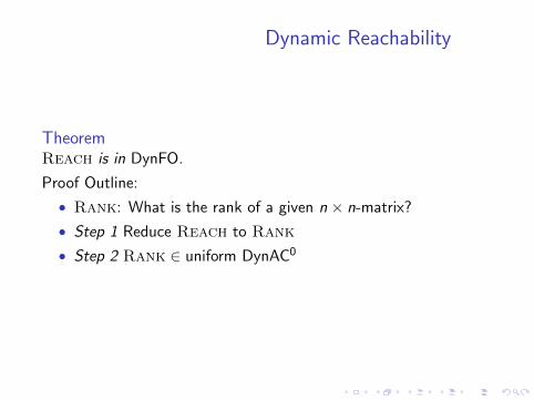
TheoremReach is in DynFO.
Proof Outline:
• Rank: What is the rank of a given n × n-matrix?
• Step 1 Reduce Reach to Rank
• Step 2 Rank ∈ uniform DynAC0
• Step 3 DynFO ≈ uniform DynAC0
Dynamic Reachability
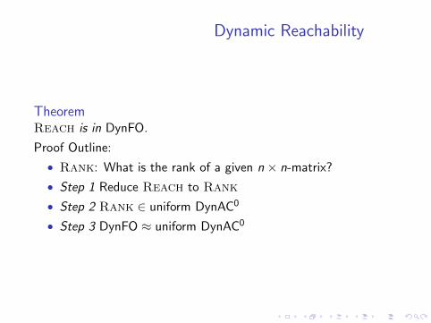
TheoremReach is in DynFO.
Proof Outline:
• Rank: What is the rank of a given n × n-matrix?
• Step 1 Reduce Reach to Rank
• Step 2 Rank ∈ uniform DynAC0
• Step 3 DynFO ≈ uniform DynAC0
Dynamic Reachability
TheoremReach is in DynFO.
Proof Outline:
• Rank: What is the rank of a given n × n-matrix?
• Step 1 Reduce Reach to Rank
• Step 2 Rank ∈ uniform DynAC0
• Step 3 DynFO ≈ uniform DynAC0
Dynamic Reachability
TheoremReach is in DynFO.
Proof Outline:
• Rank: What is the rank of a given n × n-matrix?
• Step 1 Reduce Reach to Rank
• Step 2 Rank ∈ uniform DynAC0
• Step 3 DynFO ≈ uniform DynAC0
Reducing Reach to Rank
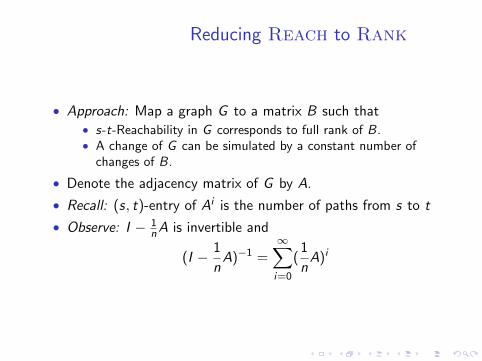
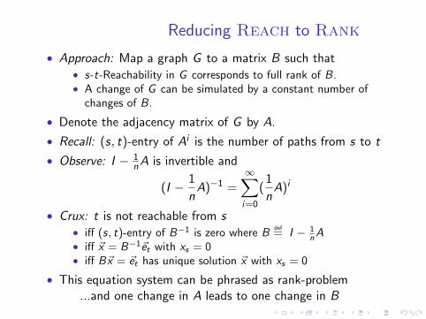
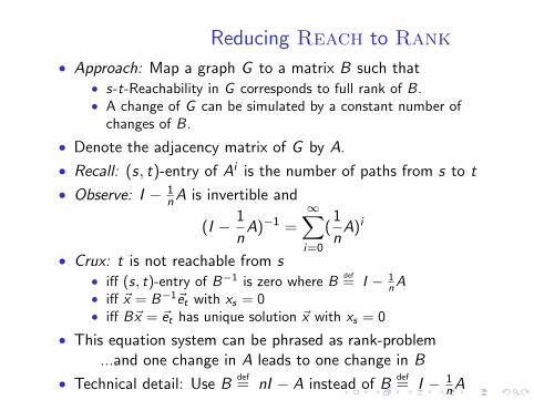
• Approach: Map a graph G to a matrix B such that• s-t-Reachability in G corresponds to full rank of B.• A change of G can be simulated by a constant number of
changes of B.
Reducing Reach to Rank
• Approach: Map a graph G to a matrix B such that• s-t-Reachability in G corresponds to full rank of B.• A change of G can be simulated by a constant number of
changes of B.
• Denote the adjacency matrix of G by A.
• Recall: (s, t)-entry of Ai is the number of paths from s to t
• Observe: I − 1nA is invertible and
(I − 1
nA)−1 =
∞∑i=0
(1
nA)i
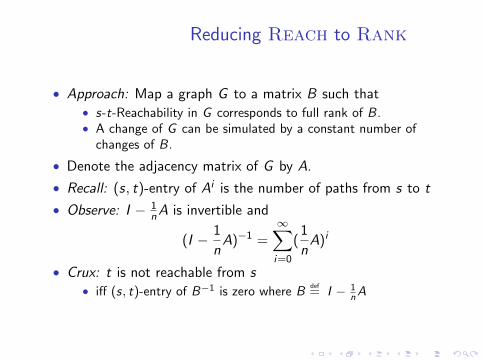
• Crux: t is not reachable from s• iff (s, t)-entry of B−1 is zero where B
def= I − 1
nA
Reducing Reach to Rank
• Approach: Map a graph G to a matrix B such that• s-t-Reachability in G corresponds to full rank of B.• A change of G can be simulated by a constant number of
changes of B.
• Denote the adjacency matrix of G by A.
• Recall: (s, t)-entry of Ai is the number of paths from s to t
• Observe: I − 1nA is invertible and
(I − 1
nA)−1 =
∞∑i=0
(1
nA)i
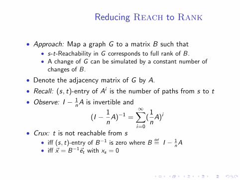
• Crux: t is not reachable from s• iff (s, t)-entry of B−1 is zero where B
def= I − 1
nA• iff ~x = B−1~et with xs = 0
Reducing Reach to Rank
• Approach: Map a graph G to a matrix B such that• s-t-Reachability in G corresponds to full rank of B.• A change of G can be simulated by a constant number of
changes of B.
• Denote the adjacency matrix of G by A.
• Recall: (s, t)-entry of Ai is the number of paths from s to t
• Observe: I − 1nA is invertible and
(I − 1
nA)−1 =
∞∑i=0
(1
nA)i
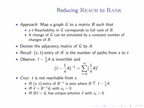
• Crux: t is not reachable from s• iff (s, t)-entry of B−1 is zero where B
def= I − 1
nA• iff ~x = B−1~et with xs = 0• iff B~x = ~et has unique solution ~x with xs = 0
Reducing Reach to Rank
• Approach: Map a graph G to a matrix B such that• s-t-Reachability in G corresponds to full rank of B.• A change of G can be simulated by a constant number of
changes of B.
• Denote the adjacency matrix of G by A.
• Recall: (s, t)-entry of Ai is the number of paths from s to t
• Observe: I − 1nA is invertible and
(I − 1
nA)−1 =
∞∑i=0
(1
nA)i
• Crux: t is not reachable from s• iff (s, t)-entry of B−1 is zero where B
def= I − 1
nA• iff ~x = B−1~et with xs = 0• iff B~x = ~et has unique solution ~x with xs = 0
• This equation system can be phrased as rank-problem...and one change in A leads to one change in B
• Technical detail: Use Bdef= nI − A instead of B
def= I − 1
nA
Reducing Rank to mod-p-Rank
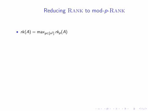
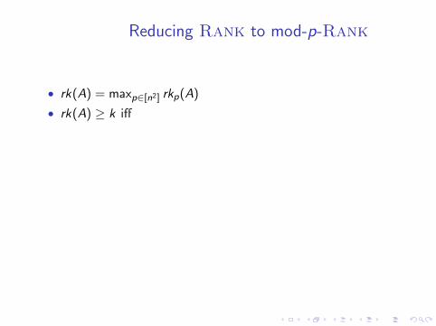
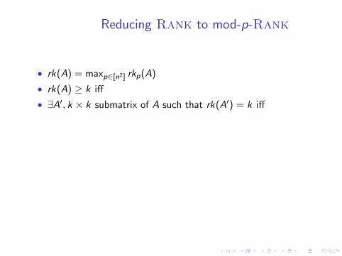
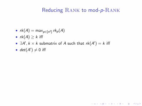
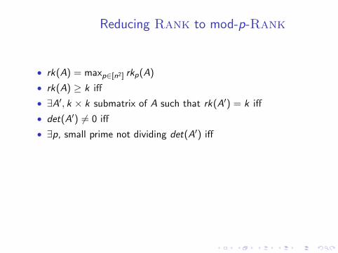
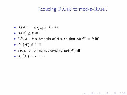
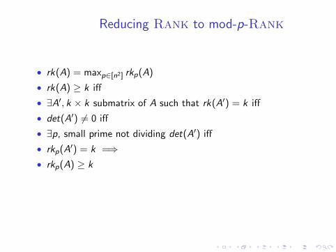
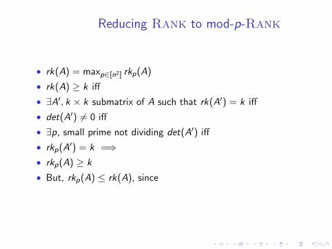
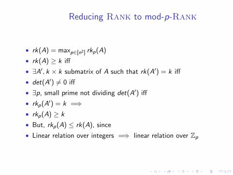
• rk(A) = maxp∈[n2] rkp(A)
• rk(A) ≥ k iff
• ∃A′, k × k submatrix of A such that rk(A′) = k iff
• det(A′) 6= 0 iff
• ∃p, small prime not dividing det(A′) iff
• rkp(A′) = k =⇒• rkp(A) ≥ k
• But, rkp(A) ≤ rk(A), since
• Linear relation over integers =⇒ linear relation over Zp
Reducing Rank to mod-p-Rank
• rk(A) = maxp∈[n2] rkp(A)
• rk(A) ≥ k iff
• ∃A′, k × k submatrix of A such that rk(A′) = k iff
• det(A′) 6= 0 iff
• ∃p, small prime not dividing det(A′) iff
• rkp(A′) = k =⇒
• rkp(A) ≥ k
• But, rkp(A) ≤ rk(A), since
• Linear relation over integers =⇒ linear relation over Zp
Reducing Rank to mod-p-Rank
• rk(A) = maxp∈[n2] rkp(A)
• rk(A) ≥ k iff
• ∃A′, k × k submatrix of A such that rk(A′) = k iff
• det(A′) 6= 0 iff
• ∃p, small prime not dividing det(A′) iff
• rkp(A′) = k =⇒• rkp(A) ≥ k
• But, rkp(A) ≤ rk(A), since
• Linear relation over integers =⇒ linear relation over Zp
Reducing Rank to mod-p-Rank
• rk(A) = maxp∈[n2] rkp(A)
• rk(A) ≥ k iff
• ∃A′, k × k submatrix of A such that rk(A′) = k iff
• det(A′) 6= 0 iff
• ∃p, small prime not dividing det(A′) iff
• rkp(A′) = k =⇒• rkp(A) ≥ k
• But, rkp(A) ≤ rk(A), since
• Linear relation over integers =⇒ linear relation over Zp
Maintaining row-echelon form
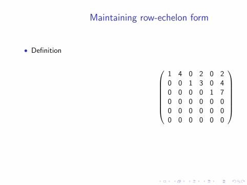
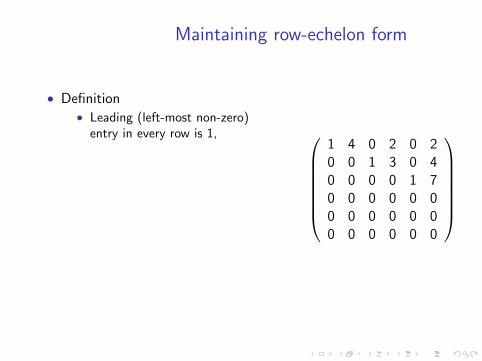
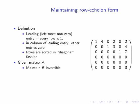
• Definition
• Leading (left-most non-zero)entry in every row is 1,
• in column of leading entry: otherentries zero
• Rows are sorted in “diagonal”fashion
• Given matrix A
• Maintain B invertible• Maintain E in row echelon form• such that E = BA
• Rank(A) is #non-zero rows of E
1 4 0 2 0 20 0 1 3 0 40 0 0 0 1 70 0 0 0 0 00 0 0 0 0 00 0 0 0 0 0
Maintaining row-echelon form
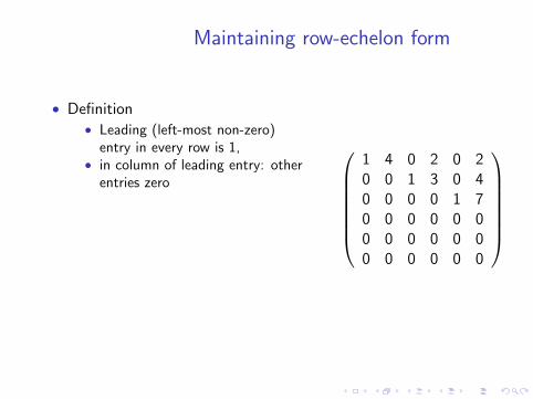
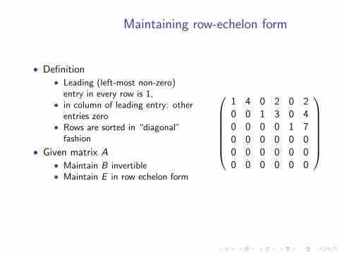
• Definition• Leading (left-most non-zero)
entry in every row is 1,
• in column of leading entry: otherentries zero
• Rows are sorted in “diagonal”fashion
• Given matrix A
• Maintain B invertible• Maintain E in row echelon form• such that E = BA
• Rank(A) is #non-zero rows of E
1 4 0 2 0 20 0 1 3 0 40 0 0 0 1 70 0 0 0 0 00 0 0 0 0 00 0 0 0 0 0
Maintaining row-echelon form
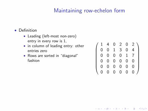
• Definition• Leading (left-most non-zero)
entry in every row is 1,• in column of leading entry: other
entries zero
• Rows are sorted in “diagonal”fashion
• Given matrix A
• Maintain B invertible• Maintain E in row echelon form• such that E = BA
• Rank(A) is #non-zero rows of E
1 4 0 2 0 20 0 1 3 0 40 0 0 0 1 70 0 0 0 0 00 0 0 0 0 00 0 0 0 0 0
Maintaining row-echelon form
• Definition• Leading (left-most non-zero)
entry in every row is 1,• in column of leading entry: other
entries zero• Rows are sorted in “diagonal”
fashion
• Given matrix A
• Maintain B invertible• Maintain E in row echelon form• such that E = BA
• Rank(A) is #non-zero rows of E
1 4 0 2 0 20 0 1 3 0 40 0 0 0 1 70 0 0 0 0 00 0 0 0 0 00 0 0 0 0 0
Maintaining row-echelon form
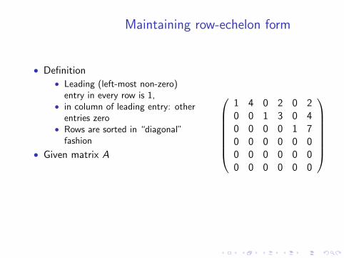
• Definition• Leading (left-most non-zero)
entry in every row is 1,• in column of leading entry: other
entries zero• Rows are sorted in “diagonal”
fashion
• Given matrix A
• Maintain B invertible• Maintain E in row echelon form• such that E = BA
• Rank(A) is #non-zero rows of E
1 4 0 2 0 20 0 1 3 0 40 0 0 0 1 70 0 0 0 0 00 0 0 0 0 00 0 0 0 0 0
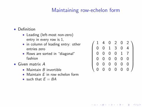
Maintaining row-echelon form
• Definition• Leading (left-most non-zero)
entry in every row is 1,• in column of leading entry: other
entries zero• Rows are sorted in “diagonal”
fashion
• Given matrix A• Maintain B invertible
• Maintain E in row echelon form• such that E = BA
• Rank(A) is #non-zero rows of E
1 4 0 2 0 20 0 1 3 0 40 0 0 0 1 70 0 0 0 0 00 0 0 0 0 00 0 0 0 0 0
Maintaining row-echelon form
• Definition• Leading (left-most non-zero)
entry in every row is 1,• in column of leading entry: other
entries zero• Rows are sorted in “diagonal”
fashion
• Given matrix A• Maintain B invertible• Maintain E in row echelon form
• such that E = BA
• Rank(A) is #non-zero rows of E
1 4 0 2 0 20 0 1 3 0 40 0 0 0 1 70 0 0 0 0 00 0 0 0 0 00 0 0 0 0 0
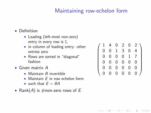
Maintaining row-echelon form
• Definition• Leading (left-most non-zero)
entry in every row is 1,• in column of leading entry: other
entries zero• Rows are sorted in “diagonal”
fashion
• Given matrix A• Maintain B invertible• Maintain E in row echelon form• such that E = BA
• Rank(A) is #non-zero rows of E
1 4 0 2 0 20 0 1 3 0 40 0 0 0 1 70 0 0 0 0 00 0 0 0 0 00 0 0 0 0 0
Maintaining row-echelon form
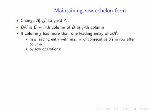
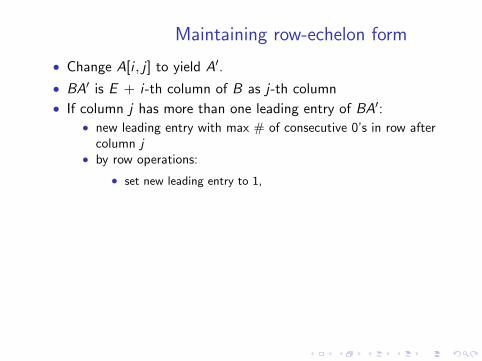
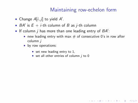
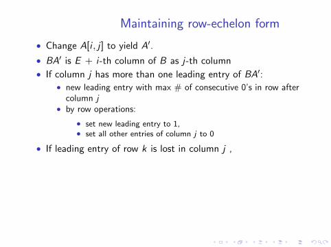
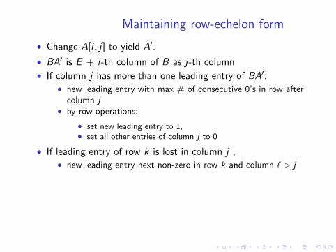
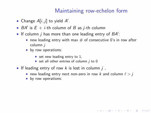
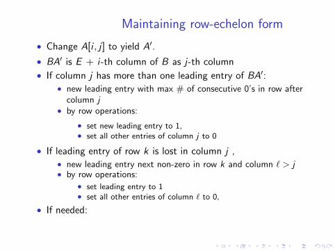
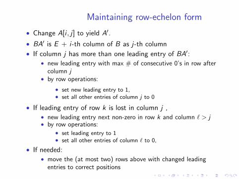
• Change A[i , j ] to yield A′.
• BA′ is E + i-th column of B as j-th column
• If column j has more than one leading entry of BA′:
• new leading entry with max # of consecutive 0’s in row aftercolumn j
• by row operations:
• set new leading entry to 1,• set all other entries of column j to 0
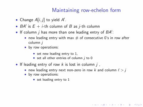
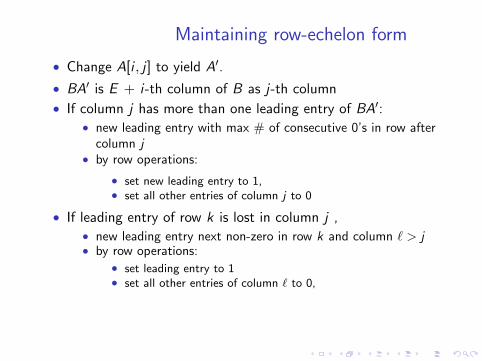
• If leading entry of row k is lost in column j ,
• new leading entry next non-zero in row k and column ` > j• by row operations:
• set leading entry to 1• set all other entries of column ` to 0,
• If needed:
• move the (at most two) rows above with changed leadingentries to correct positions
Maintaining row-echelon form
• Change A[i , j ] to yield A′.
• BA′ is E + i-th column of B as j-th column
• If column j has more than one leading entry of BA′:
• new leading entry with max # of consecutive 0’s in row aftercolumn j
• by row operations:
• set new leading entry to 1,• set all other entries of column j to 0
• If leading entry of row k is lost in column j ,
• new leading entry next non-zero in row k and column ` > j• by row operations:
• set leading entry to 1• set all other entries of column ` to 0,
• If needed:
• move the (at most two) rows above with changed leadingentries to correct positions
Maintaining row-echelon form
• Change A[i , j ] to yield A′.
• BA′ is E + i-th column of B as j-th column
• If column j has more than one leading entry of BA′:• new leading entry with max # of consecutive 0’s in row after
column j
• by row operations:
• set new leading entry to 1,• set all other entries of column j to 0
• If leading entry of row k is lost in column j ,
• new leading entry next non-zero in row k and column ` > j• by row operations:
• set leading entry to 1• set all other entries of column ` to 0,
• If needed:
• move the (at most two) rows above with changed leadingentries to correct positions
Maintaining row-echelon form
• Change A[i , j ] to yield A′.
• BA′ is E + i-th column of B as j-th column
• If column j has more than one leading entry of BA′:• new leading entry with max # of consecutive 0’s in row after
column j• by row operations:
• set new leading entry to 1,
• set all other entries of column j to 0
• If leading entry of row k is lost in column j ,
• new leading entry next non-zero in row k and column ` > j• by row operations:
• set leading entry to 1• set all other entries of column ` to 0,
• If needed:
• move the (at most two) rows above with changed leadingentries to correct positions
Maintaining row-echelon form
• Change A[i , j ] to yield A′.
• BA′ is E + i-th column of B as j-th column
• If column j has more than one leading entry of BA′:• new leading entry with max # of consecutive 0’s in row after
column j• by row operations:
• set new leading entry to 1,• set all other entries of column j to 0
• If leading entry of row k is lost in column j ,
• new leading entry next non-zero in row k and column ` > j• by row operations:
• set leading entry to 1• set all other entries of column ` to 0,
• If needed:
• move the (at most two) rows above with changed leadingentries to correct positions
Maintaining row-echelon form
• Change A[i , j ] to yield A′.
• BA′ is E + i-th column of B as j-th column
• If column j has more than one leading entry of BA′:• new leading entry with max # of consecutive 0’s in row after
column j• by row operations:
• set new leading entry to 1,• set all other entries of column j to 0
• If leading entry of row k is lost in column j ,• new leading entry next non-zero in row k and column ` > j
• by row operations:
• set leading entry to 1• set all other entries of column ` to 0,
• If needed:
• move the (at most two) rows above with changed leadingentries to correct positions
Maintaining row-echelon form
• Change A[i , j ] to yield A′.
• BA′ is E + i-th column of B as j-th column
• If column j has more than one leading entry of BA′:• new leading entry with max # of consecutive 0’s in row after
column j• by row operations:
• set new leading entry to 1,• set all other entries of column j to 0
• If leading entry of row k is lost in column j ,• new leading entry next non-zero in row k and column ` > j• by row operations:
• set leading entry to 1
• set all other entries of column ` to 0,
• If needed:
• move the (at most two) rows above with changed leadingentries to correct positions
Maintaining row-echelon form
• Change A[i , j ] to yield A′.
• BA′ is E + i-th column of B as j-th column
• If column j has more than one leading entry of BA′:• new leading entry with max # of consecutive 0’s in row after
column j• by row operations:
• set new leading entry to 1,• set all other entries of column j to 0
• If leading entry of row k is lost in column j ,• new leading entry next non-zero in row k and column ` > j• by row operations:
• set leading entry to 1• set all other entries of column ` to 0,
• If needed:
• move the (at most two) rows above with changed leadingentries to correct positions
Maintaining row-echelon form
• Change A[i , j ] to yield A′.
• BA′ is E + i-th column of B as j-th column
• If column j has more than one leading entry of BA′:• new leading entry with max # of consecutive 0’s in row after
column j• by row operations:
• set new leading entry to 1,• set all other entries of column j to 0
• If leading entry of row k is lost in column j ,• new leading entry next non-zero in row k and column ` > j• by row operations:
• set leading entry to 1• set all other entries of column ` to 0,
• If needed:• move the (at most two) rows above with changed leading
entries to correct positions
Outline
1 Part I: Disjoint Paths
2 Part II: Dynamic Reachability
3 Conclusion
Conclusion
• Considered two connectivity problems:
• One-face k-DPP• Dynamic Reachability
• Writing and solving linear equations, key to solution
• Scratched the surface of Linear Algebra
Conclusion
• Considered two connectivity problems:• One-face k-DPP
• Dynamic Reachability
• Writing and solving linear equations, key to solution
• Scratched the surface of Linear Algebra
Conclusion
• Considered two connectivity problems:• One-face k-DPP• Dynamic Reachability
• Writing and solving linear equations, key to solution
• Scratched the surface of Linear Algebra
Conclusion
• Considered two connectivity problems:• One-face k-DPP• Dynamic Reachability
• Writing and solving linear equations, key to solution
• Scratched the surface of Linear Algebra
Conclusion
• Considered two connectivity problems:• One-face k-DPP• Dynamic Reachability
• Writing and solving linear equations, key to solution
• Scratched the surface of Linear Algebra
Open Questions
• Derandomize construction of One-face k-DPP solution?
• “Deparameterize” counting or even decision of above?
• From 4knO(1) to kO(1)nO(1)?• Serial/parallel cases can be deparameterized [Borradaile et al.]• Contrariwise, does there exist a crossover gadget?
• Is directed distance in DynAC0? What about pathconstruction?
Open Questions
• Derandomize construction of One-face k-DPP solution?
• “Deparameterize” counting or even decision of above?• From 4knO(1) to kO(1)nO(1)?
• Serial/parallel cases can be deparameterized [Borradaile et al.]• Contrariwise, does there exist a crossover gadget?
• Is directed distance in DynAC0? What about pathconstruction?
Open Questions
• Derandomize construction of One-face k-DPP solution?
• “Deparameterize” counting or even decision of above?• From 4knO(1) to kO(1)nO(1)?• Serial/parallel cases can be deparameterized [Borradaile et al.]
• Contrariwise, does there exist a crossover gadget?
• Is directed distance in DynAC0? What about pathconstruction?
Open Questions
• Derandomize construction of One-face k-DPP solution?
• “Deparameterize” counting or even decision of above?• From 4knO(1) to kO(1)nO(1)?• Serial/parallel cases can be deparameterized [Borradaile et al.]• Contrariwise, does there exist a crossover gadget?
• Is directed distance in DynAC0? What about pathconstruction?

Thanks!