solving games and all that - accueil - tel
TRANSCRIPT

HAL Id: tel-01022750https://tel.archives-ouvertes.fr/tel-01022750
Submitted on 10 Jul 2014
HAL is a multi-disciplinary open accessarchive for the deposit and dissemination of sci-entific research documents, whether they are pub-lished or not. The documents may come fromteaching and research institutions in France orabroad, or from public or private research centers.
L’archive ouverte pluridisciplinaire HAL, estdestinée au dépôt et à la diffusion de documentsscientifiques de niveau recherche, publiés ou non,émanant des établissements d’enseignement et derecherche français ou étrangers, des laboratoirespublics ou privés.
Solving Games and All ThatAbdallah Saffidine
To cite this version:Abdallah Saffidine. Solving Games and All That. Artificial Intelligence [cs.AI]. Université ParisDauphine - Paris IX, 2013. English. �NNT : 2013PA090069�. �tel-01022750�
UNIVERSITE PARIS-DAUPHINE — ECOLE DOCTORALE DE DAUPHINE
SOLVING GAMES AND ALL THAT
ABDALLAH SAFFIDINE
MANUSCRIT POUR L’OBTENTION D’UN DOCTORAT ES SCIENCES
SPECIALITE INFORMATIQUE
8 JUILLET 2013
Tristan CAZENAVE . . . . . . . . . . . . . . . . . . . . . . . . . . . . . . . . . . . . . . . . . . . . . . . . . . Directeur de these
Stefan EDELKAMP . . . . . . . . . . . . . . . . . . . . . . . . . . . . . . . . . . . . . . . . . . . . . . . . . . . . . . . . . Rapporteur
Olivier TEYTAUD . . . . . . . . . . . . . . . . . . . . . . . . . . . . . . . . . . . . . . . . . . . . . . . . . . . . . . . . . . Rapporteur
Andreas HERZIG . . . . . . . . . . . . . . . . . . . . . . . . . . . . . . . . . . . . . . . . . . . . . . . . . . . . . .Membre du jury
Martin MULLER . . . . . . . . . . . . . . . . . . . . . . . . . . . . . . . . . . . . . . . . . . . . . . . . . . . . . . Membre du jury
Universite Paris-Dauphine
Place du Marechal de Lattre de Tassigny
75116 Paris, France


Abstract
Efficient best-first search algorithms have been developed for determin-
istic two-player games with two outcomes. We present a formal framework
to represent such best-first search algorithms. The framework is general
enough to express popular algorithms such as Proof Number Search, Monte
Carlo Tree Search, and the Product Propagation algorithm. We then show
how a similar framework can be devised for two more general settings:
two-player games with multiple outcomes, and the model checking problem
in modal logic K. This gives rise to new Proof Number and Monte Carlo
inspired search algorithms for these settings.
Similarly, the alpha-beta pruning technique is known to be very impor-
tant in games with sequential actions. We propose an extension of this
technique for stacked-matrix games, a generalization of zero-sum perfect
information two-player games that allows simultaneous moves.
Keywords: Artificial Intelligence, Monte Carlo Tree Search, Proof Number
Search, Modal Logic K, Alpha-beta Pruning
Resume
Il existe des algorithmes en meilleur d’abord efficace pour la resolution
des jeux deterministes a deux joueurs et a deux issues. Nous proposons un
cadre formel pour la representation de tels algorithms en meilleur d’abord.
Le cadre est suffisamment general pour exprimer des algorithmes populaires
tels Proof Number Search, Monte Carlo Tree Search, ainsi que l’algorithme
Product Propagation. Nous montrons par ailleurs comment adapter ce cadre
a deux situations plus generales : les jeux a deux-joueurs a plusieurs issues,
et le probleme de model checking en logique modale K. Cela donne lieu a
de nouveaux algorithmes pour ces situations inspirees des methodes Proof
Number et Monte Carlo.
La technique de l’elagage alpha-beta est cruciale dans les jeux a actions
sequentielles. Nous proposons une extension de cette technique aux stacked-
matrix games, une generalisation des jeux a deux joueurs, a information
parfaite et somme nulle qui permet des actions simultanees.
Mots cles : Intelligence Artificielle, Monte Carlo Tree Search, Proof Number
Search, Logique Modale K, Elagage Alpha-beta
i

Contents
Contents ii
Acknowledgments v
1 Introduction 1
1.1 Motivation . . . . . . . . . . . . . . . . . . . . . . . . . . . . . . 1
1.2 Organization and Contributions . . . . . . . . . . . . . . . . . . 3
1.3 Contributions not detailed in this thesis . . . . . . . . . . . . . . 5
1.4 Basic Notions and Notations . . . . . . . . . . . . . . . . . . . . 14
2 Two-Outcome Games 17
2.1 Game Model . . . . . . . . . . . . . . . . . . . . . . . . . . . . 18
2.2 Depth First Search . . . . . . . . . . . . . . . . . . . . . . . . . 23
2.3 Best First Search . . . . . . . . . . . . . . . . . . . . . . . . . . 26
2.4 Proof Number Search . . . . . . . . . . . . . . . . . . . . . . . . 31
2.5 Monte Carlo Tree Search . . . . . . . . . . . . . . . . . . . . . . 34
2.6 Product Propagation . . . . . . . . . . . . . . . . . . . . . . . . 36
3 Multi-Outcome Games 45
3.1 Introduction . . . . . . . . . . . . . . . . . . . . . . . . . . . . . 46
3.2 Model . . . . . . . . . . . . . . . . . . . . . . . . . . . . . . . . 47
3.3 Iterative perspective . . . . . . . . . . . . . . . . . . . . . . . . 48
3.4 MiniMax and Alpha-Beta . . . . . . . . . . . . . . . . . . . . . . 49
3.5 Multiple-Outcome Best First Search . . . . . . . . . . . . . . . . 49
3.6 Multization . . . . . . . . . . . . . . . . . . . . . . . . . . . . . 58
ii

Contents
3.7 Multiple-Outcome Proof Number Search . . . . . . . . . . . . . 60
3.8 Experimental results . . . . . . . . . . . . . . . . . . . . . . . . 64
3.9 Conclusion and discussion . . . . . . . . . . . . . . . . . . . . . 69
4 Modal Logic K Model Checking 71
4.1 Introduction . . . . . . . . . . . . . . . . . . . . . . . . . . . . . 72
4.2 Definitions . . . . . . . . . . . . . . . . . . . . . . . . . . . . . . 74
4.3 Model Checking Algorithms . . . . . . . . . . . . . . . . . . . . 80
4.4 Minimal Proof Search . . . . . . . . . . . . . . . . . . . . . . . 85
4.5 Sequential solution concepts in MMLK . . . . . . . . . . . . . . . 94
4.6 Understanding game tree algorithms . . . . . . . . . . . . . . . 98
4.7 Related work and discussion . . . . . . . . . . . . . . . . . . . . 104
4.8 Conclusion . . . . . . . . . . . . . . . . . . . . . . . . . . . . . 107
5 Games with Simultaneous Moves 109
5.1 Stacked-matrix games . . . . . . . . . . . . . . . . . . . . . . . 110
5.2 Solution Concepts for Stacked-matrix Games . . . . . . . . . . . 115
5.3 Simultaneous Move Pruning . . . . . . . . . . . . . . . . . . . . 120
5.4 Fast approximate search for combat games . . . . . . . . . . . . 128
5.5 Experiments . . . . . . . . . . . . . . . . . . . . . . . . . . . . . 133
5.6 Conclusion and Future Work . . . . . . . . . . . . . . . . . . . . 139
6 Conclusion 143
A Combat game abstract model 145
Bibliography 147
iii


Acknowledgments
My doctoral studies have come to a happy conclusion. As I contemplate the
journey, I see that a score of people have had a distinct positive influence on my
last three years. I cannot list the name of every single person that I am grateful
to, but I will try to exhibit a representative sample.
Tristan Cazenave, you are passionate about games and artificial intelligence,
hard-working, and yet you manage to lead a balanced life. More than a research
advisor, you have been a role model. The more I observe you, the more I know
I want to be an academic.
Stefan Edelkamp and Olivier Teytaud, you immediately agreed to review
my thesis despite your busy schedule and you provided valuable feedback.
Discussing with you has always been enlightening and I look forward to starting
working with you. Andreas Herzig and Martin Muller, you accepted to serve on
my thesis committee. I am also thankful for the short and long research visits
that I made in your respective groups.
Mohamed-Ali Aloulou, Cristina Bazgan, Denis Bouyssou, Virginie Gabrel,
Vangelis Paschos, and Alexis Tsoukias, be it for books, for conferences, research
visits, or even to go spend a year in another university on another continent, I
was always generously supported.
Caroline Farge, Valerie Lamauve, Mireille Le Barbier, Christine Vermont,
and the other staff from University Paris-Dauphine, everyday, you build bridges
between the bureaucracy and the absent-minded researchers and students so
that the administrative labyrinth becomes less of a hassle. In particular Katerina
Kinta, Nathalie Paul de la Neuville, and Olivier Rouyer, you always spent the
time needed to solve my daily riddles, even when the situation was complicated
v

ACKNOWLEDGMENTS
or didn’t make sense.
Jerome Lang, you introduced me to another research community and acted
as a mentor giving me advice and answering my many questions about the
research process. Hans van Ditmarsch, from the day we met, you treated me
like a colleague rather than a student, it surely helped me gain confidence.
Flavien Balbo, Edouard Bonnet, Denis Cornaz, and Suzanne Pinson, you trusted
me and teaching for/with you was a real pleasure.
Michael Bowling, Michael Buro, Ryan Hayward, Mike Johanson, Martin
Muller, Rick Valenzano and the members of the Hex, Heuristic Search, Monte
Carlo, Poker, and Skat Meeting Groups, with you I benefited from an unlimited
supply of ideas and insights.
My coauthors, Chris Archibald, Edouard Bonnet, Michael Buro, Cedric Buron,
Tristan Cazenave, Dave Churchill, Hans van Ditmarsch, Edith Elkind, Hilmar
Finnsson, Florian Jamain, Nicolas Jouandeau, Marc Lanctot, Jerome Lang, Jean
Mehat, Michael Schofield, Joel Veness, and Mark Winands, as well as other
people I have collaborated with, for your creative input.
Nathanael Barrot, Amel Benhamiche, Morgan Chopin, Miguel Couceiro,
Tom Denat, Eunjung Kim, Renaud Lacour, Dalal Madakat, Mohamed Amine
Mouhoub, Nicolas Paget, Lydia Tlilane, and the other CS faculty, PhD students,
interns, and alumni in Dauphine, you all contributed to a friendly and wel-
coming atmosphere in our workplace. Emeric Tourniaire, you recognize that
form matters and you were always ready to help improve my presentation and
typography skills. Raouia Taktak, somehow it always was comforting to meet
you in the hallway in the middle of the night as we both tried to finish writing
our respective dissertations.
Anthony Bosse and Camille Crepon, you were there in the bad times and
you were there in the good times, I am lucky to count you among my friends.
Vincent Nimal, you always were in an another country but I knew I could reach
you and talk to you any time I wanted. Sarah Juma, with your patience and
understanding, I have learned more than any higher education can provide.
Marc Bellemare, thank you for the welcome you gave me in Edmonton when
I arrived in your country and in Quebec when I was about to leave it, you’ve
been so helpful all the way long. James, Mohsen, and Nikos, living, drinking,
cooking, and watching movies with you guys made Canada feel home despite
the cold winter.
vi

Felicity Allen, Marc Bellemare, Edouard Bonnet, Dave Churchill, Tim Furtak,
Richard Gibson, Florian Jamain, Marc Lanctot, Arpad Rimmel, Fabien Teytaud,
Joel Veness, you were always ready to play, be it abstract games, board games,
card games, or video games. Michael Buro, Rob Holte, and Jonathan Scha-
effer, the GAMES parties you organized are among my favorite memories of
Edmonton.
Bonita Akai, Eric Smith, and the members of the University of Alberta Improv
Group, it was a lot of fun to spend time with you and you definitely contributed
to the balance of my Canadian life. Pierre Puy, Richard Soudee, and the member
of the Association de Theatre a Dauphine, I enjoyed spending those Friday
evenings and nights with you.
Pilar Billiet and Mate Rabinovski, whenever I needed to escape my Parisian
routine, you offered me a quiet, cultural, and gastronomical break. Therese
Baskoff, Helene and Matthieu Brochard, Daniele Geesen, and Monique Nybelen,
without you, the final day of my PhD would have been much less enjoyable.
Thank you for your help.
My grand-parents, Grand-Mere, for your jokes, always unexpected and
creative, and Grand-Pere, for your experienced input and sharp guidance,
always relevant. Mum and Dad, you always cared to make your work and
projects accessible to other people. Thank you for showing me that there is
much fun to be found at work. Sonya, my sister, with such a positive bias in
your eyes, I can only feel better when you talk to me.
Finally, I would also like to express a thought for Hamid, Nabila, Pierrot,
Thierry, and the rest of my family whom I haven’t seen much in the last few years,
for Jonathan Protzenko, Sebastien Tavenas, Jorick Vanbeselaere, Sebastien
Wemama, and my other friends, for those too few but cheering and joyful times.
vii


1 Introduction
1.1 Motivation
The term multi-agent system has been used in many different situations and
it does not correspond to a single unified formalism. Indeed, formal concepts
such as extensive-form games, multi-agent environments, or Kripke structures
can all be thought of as referring to some kind of multi-agent system.
A large fraction of the multi-agent systems lend themselves to a multi-stage
interpretation. This multi-stage interpretation is non only relevant in domains
where agents perform actions sequentially, but also, say, in epistemic logics
where agents can have higher order knowledge/beliefs or perform introspection.
The underlying structure of these multi-stage problems is that of a graph where
the vertex correspond to states of the world and the edges correspond to the
actions the agents can take or to the applications of modal operators in epistemic
logic.
Properties of the system can thus be reduced to properties of the underlying
graph. The algorithmic stance adopted in this thesis consists of expressing
concrete heuristics or algorithms that allow to understand a multi-agent system
through the exploration of the corresponding graph. In most non-trivial such
multi-agent systems, the underlying graph is too large to be kept in memory
and explored fully. This consideration gives rise to the Search paradigm. In
Search, the graph is represented implicitly, typically with some starting vertex
and a successor function that returns edges or vertices adjacent to its argument.
Opposite to this high-level description of search problems in general, we
have a variety of concrete applications, research communities, and, accordingly,
1

1. INTRODUCTION
typical assumptions on the graphs of interest. As a result, many classical search
algorithms are developed with these assumptions in mind and seem to be
tailored to a specific class of multi-agent systems. The conducting line of our
work is to study whether and how such algorithms can be generalized and some
assumptions lifted so as to encompass a larger class of multi-agent systems.
The research presented in this thesis has two main starting points, the alpha-
pruning technique for the depth-first search algorithm known as minimax on
the one hand, and the Monte Carlo Tree Search (MCTS) and Proof Number
Search (PNS) algorithms on the other hand.
The minimax algorithm which is a generalization of depth-first search to
sequential two-player zero-sum games can be significantly improved by the
alpha-beta pruning technique. Alpha-beta pruning avoids searching subtrees
which are provably not needed to solve the problem at hand. Two important
facts contribute to the popularity of alpha-beta pruning in game search. It is
a safe pruning technique in that the result returned by the depth-first search
is not affected when pruning is enabled. Discarding subtrees according to
the alpha-beta pruning criterion can lead to considerable savings in terms of
running time. Indeed, Knuth and Moore have shown that if a uniform tree of
size n was explored by the minimax algorithm, alpha-beta pruning might only
necessitate the exploration of a subtree of size√n.
Alpha-beta pruning contributed to the creating of very strong artificial
players in numerous games from CHESS to OTHELLO. However, the original
algorithm for alpha-beta pruning only applied to deterministic sequential zero-
sum two-player games of perfect information (called multi-outcome games
in this thesis, see Chapter 3). This is quite a strong restriction indeed and
there have been many attempts at broadening the class of multi-agent systems
that can benefit from alpha-beta-like safe pruning. Ballard and Hauk et al.
have shown how to relax the deterministic assumption so that safe pruning
could be applied to stochastic sequential zero-sum two-player games of perfect
information [13, 61]. Sturtevant has then shown how the two-player and the
zero-sum assumptions could be alleviated [147, 148]. In Chapter 5, we lift the
sequentiality assumption and show how safe alpha-beta-style pruning can be
performed in zero-sum two-player games with simultaneous moves. Thus, two
tasks remain to be completed before safe alpha-beta pruning can be applied to
a truly general class of multi-agent system. Creating a unified formalism that
2
1.2. Organization and Contributions
would allow combining the aforementioned techniques and providing pruning
criteria for imperfect information games in extensive-form.
The PNS and MCTS algorithms were first suggested as ways to respectively
solve and play deterministic sequential two-player Win/Loss games of perfect
information (called two-outcome games in this thesis, see Chapter 2). Both
algorithms proved very successful at their original tasks. Variants of PNS [74]
were essential to solve a number of games, among which CHECKERS [136],
FANORONA [131], as well as medium sizes of HEX [8]. On the other hand, the
invention of the Upper Confidence bound for Trees (UCT) [76] and MCTS [40]
algorithms paved the way for the Monte Carlo revolution that improved consid-
erably the computer playing level in a number of games, including GO [85],
HEX [7], and General Game Playing (GGP) [47] (see the recent survey by Browne
et al. for an overview [20]).
Besides actual games, these algorithms have been used in other settings that
can be represented under a similar formalism, notably chemical synthesis [64]
and energy management problems [39].
In their simplest form, the PNS and MCTS algorithms maintain a partial game
tree in memory and they share another important feature. They can be both
expressed as the iteration of the following four-step process: descend the tree
until a leaf is reached, expand the leaf, collect some information on the new
generated leaves, backpropagate this information in the tree up to the root.
This leads us to define a Best First Search (BFS) framework consisting exactly
of these four steps and parameterized by an information scheme. The information
scheme determines the precise way the tree is to be traverse, the kind of
information collected at leaves and how information is backpropagated. The
BFS framework is first defined in Chapter 2 for two-outcome games and then
extended to multi-outcome games and to Multi-agent Modal Logic K (MMLK)
model checking.
1.2 Organization and Contributions
The common formalism used throughout this thesis is the transition system (see
Definition 1 in Section 1.4). Transition systems have been used in a variety
of domains, and particularly in verification and model checking [11]. In this
thesis, we shall focus on a few selected classes of multi-agent systems for which
3

1. INTRODUCTION
we will present and develop appropriate solving techniques. Each chapter of
this thesis is organized around a specific class and we will see how they can all
be viewed as particular transition systems where a few additional assumptions
hold.
Chapter 2 Two-player two-outcome games
Chapter 3 Two-player multi-outcome games
Chapter 4 Models of Multi-agent Modal Logic K
Chapter 5 Stacked-matrix games
More precisely, the contributions presented in this thesis include
• – A formal BFS framework for two-outcome games based on the new
concept of information scheme;
– information schemes generating the PNS, MCTS Solver, and Product
Propagation (PP) algorithms;
– an experimental investigation of PP demonstrating that PP can some-
times perform significantly better than the better known algorithms
PNS and MCTS;
• – an extension of the BFS framework to multi-outcome games through
the new concept of multi-outcome information scheme;
– an information scheme defining the Score Bounded Monte Carlo Tree
Search (SBMCTS) algorithm, a generalization of MCTS Solver;
– a principled approach to transforming a two-outcome information
scheme into a multi-outcome information scheme;
– the application of this approach to develop Multiple-Outcome Proof
Number Search (MOPNS), a generalization of PNS to multi-outcome
games and an experimental study of MOPNS;
• – an adaptation of the proposed BFS framework to the model checking
problem in MMLK, yielding several new model checking algorithms
for MMLK;
4

1.3. Contributions not detailed in this thesis
– Minimal Proof Search (MPS), an optimal algorithm to find (dis)proofs
of minimal size for the model checking problem in MMLK.
– a formal definition of many solution concepts popular in sequential
games via MMLK formula classes, including ladders in two-player
games, and paranoid wins in multi-player games;
– the use of MMLK reasoning to prove formal properties about these
solution concepts and to provide a classification of number of algo-
rithms for sequential games;
• – a generalization of Alpha-Beta pruning in games with simultaneous
moves, Simultaneous Move Alpha-Beta (SMAB);
– an efficient heuristic algorithm for games with simultaneous moves
under tight time constraints in the domain of Real-Time Strategy
(RTS) games, Alpha-Beta (Considering Durations) (ABCD);
– an experimental investigation of these new algorithms.
1.3 Contributions not detailed in this thesis
1.3.1 Endgames and retrograde analysis
The algorithms presented in this thesis are based on forward search. Given
an initial state s0, they try to compute some property of s0, typically its game
theoretic value, by examining states that can be reached from s0.
It is sometimes possible to statically, i.e., without search, compute the game
theoretic value of a game position even though it might no be a final position.
We developed a domain specific technique for the game of BREAKTHROUGH
called race patterns that allows to compute the winner of positions that might
need a dozen additional moves before the winner can reach a final state [126].
We also proposed a parallelization of the PN2 algorithm on a distributed system
in a fashion reminiscent of Job-Level Proof Number Search [168]. An imple-
mentation of race patterns and the parallelization of PN2 on a 64-client system
allowed us to solve BREAKTHROUGH positions up to size 6× 5 while the largest
position solved before was 5× 5.
An interesting characteristic of a number of domains that we try to solve is
that they are convergent, that is, there are few states in the endgames compared
5

1. INTRODUCTION
to the middle game. For example, CHESS is convergent as the number of possible
states shrinks as the number of pieces on the board decreases. It is possible to
take advantage of this characteristic by building endgame databases that store
the game theoretic value of endgame positions that have been precomputed.
In CHESS, endgame databases, or rather one particularly efficient encoding
called Nalimov tables, are now pervasive and used by every competitive CHESS
playing engine [152, 104]. Endgame databases have been crucial to solving
other games such as CHECKERS [135], AWARI [116], and FANORONA [131].
An endgame database does actually not need to contain all endgame posi-
tions but only a representative position for every symmetry equivalence class.
Geometrical symmetry is the most common type of symmetry and it typically
involves flipping or rotating the game board [42]. Another kind of symmetry
occur in trick-taking card games, where different cards can take corresponding
roles. We call this it material symmetry and we show argue that it occurs in a
variety of games besides trick-taking card games.
We argue that material symmetry can often be detected via the graph
representing the possible interaction of the different game elements (the mate-
rial) [128]. Indeed, we show in three different games, SKAT, DOMINOES, and
CHINESE DARK CHESS that material symmetry reduces to the subgraph isomor-
phism problem in the corresponding interaction graph. Our method yields
a principled and relatively domain-agnostic approach to detecting material
symmetry that can leverage graph theory research [154]. While creating a
domain-specific algorithm for detecting material symmetry in SKAT and DOMI-
NOES is not hard, interactions between pieces in CHINESE DARK CHESS are
quite intricate and earlier work on CHINESE DARK CHESS discarded any material
symmetry. On the other hand, the interaction graph follows directly from the
rules of the game and we show that material symmetry can lead to equivalent
databases that are an order of magnitude smaller.
[126] Abdallah Saffidine, Nicolas Jouandeau, and Tristan Cazenave. Solv-
ing Breakthough with race patterns and Job-Level Proof Number Search.
In H. van den Herik and Aske Plaat, editors, Advances in Computer
Games, volume 7168 of Lecture Notes in Computer Science, pages 196–207.
Springer-Verlag, Berlin / Heidelberg, November 2011. ISBN 978-3-642-
31865-8. doi: 10.1007/978-3-642-31866-5 17
6
1.3. Contributions not detailed in this thesis
[128] Abdallah Saffidine, Nicolas Jouandeau, Cedric Buron, and Tristan
Cazenave. Material symmetry to partition endgame tables. In 8th In-
ternational Conference on Computers and Games (CG). Yokohama, Japan,
August 2013
1.3.2 Monte Carlo Methods
Monte Carlo methods are being more and more used for game tree search.
Besides the Score Bounded Monte Carlo Tree Search algorithm that we detail in
Chapter 3, we have investigated two aspects of these Monte Carlo methods. In
a first line of work, we focused on the MCTS algorithm and studied how trans-
positions could be taken into account [125]. After showing a few theoretical
shortcomings of some naive approaches to handling transpositions, we proposed
a parameterized model to use transposition information. The parameter space
of our model is general enough to represent the naive approach used in most
implementations of the MCTS algorithm, the alternative algorithms proposed
by Childs et al. [27], as well a whole range of new settings. In an extensive
experimental study ranging over a dozen domains we show that it is consistently
possible to improve upon the standard way of dealing with transposition. That
is, we show that the parameter setting simulating the standard approaches
almost always perform significantly worse than the optimal parameter setting.
In a second line of work, we propose a new Monte Carlo algorithm for
stochastic two-player games with a high branching factor at chance nodes [83].
The algorithms we propose are quite similar to EXPECTIMAX and its pruning
variants STAR1 and STAR2 [61]. The only difference is that instead of looping
over all possible moves at a chance nodes, we sample a bounded subset of moves.
This allows searching faster or much deeper trees at the cost of some inaccuracy
in the computed value. We show that the computed value is accurate with a
high probability that does not depend on the true branching factor at chance
nodes. This results constitute a generalization of sparse sampling from Markov
Decision Processes to stochastic adversarial games [72]. It can also be related to
the double progressive widening idea [38]. We conduct an experimental study
on four games and show that the new approach consistently outperforms their
non-sampling counterparts.
[125] Abdallah Saffidine, Tristan Cazenave, and Jean Mehat. UCD: Upper
7

1. INTRODUCTION
Confidence bound for rooted Directed acyclic graphs. Knowledge-Based
Systems, 34:26–33, December 2011. doi: 10.1016/j.knosys.2011.11.014
[83] Marc Lanctot, Abdallah Saffidine, Joel Veness, Chris Archibald, and
Mark Winands. Monte carlo *-minimax search. In 23rd International Joint
Conference on Artificial Intelligence (IJCAI), Beijing, China, August 2013.
AAAI Press
1.3.3 Analysis of the Game Description Language
The formalism use throughout this thesis is based on transition systems. These
transition systems notably include a state space and a transition relation. How-
ever, in practice the state space is implicit and uses a domain specific state
representation. In that case, the transition relation is given by domain specific
game rules.
The most straightforward approach to running concrete algorithms on a
domain, is to implement the mechanics of the domain directly in some program-
ming language and to provide procedure to manipulate states in a specified
interface. The algorithms to be tested are implemented in the same program-
ming language and can be adapted to use the specified interface.
One downside to this approach is that describing game rules in the same
procedural language as the algorithms might be tedious for some games. Even
more so, this approach makes automatic comparison between competing al-
gorithms implemented by different people rather difficult. Indeed, when we
compare two implementations of two competing algorithms based on two dif-
ferent implementation of the domain, determining whether a speed-up is due
to an improvement on the algorithm side or is due to a domain-specific trick is
usually tricky, particularly when the implementations are not publicly available.
An alternative approach is to develop a standard modeling language to
represent domains and then have interfaces from the language of the domains
to the programming language of the algorithms. We can then measure the
merits of various algorithms on the very same domain without fear that domain
specific improvements might creep in some implementations only.
This idea was successfully brought into effect in multiple research communi-
ties. For instance, the PROMELA language was designed to represent distributed
system and makes it possible to implement model checking or verification
8

1.3. Contributions not detailed in this thesis
algorithms in a domain agnostic way [67, 68]. In planning, the Planning Do-
main Description Language (PDDL) was developed to be used as part of the
international planning competitions [48, 65].
In the games community, the Game Description Language (GDL) was in-
troduced to model a large variety of multi-agent transition systems [93]. GDL
was used as a domain language in the yearly GGP competition and hundreds of
games have been specified in this language. Interfacing domain written in GDL
with a game playing engine is traditionally based on a Prolog interpreter such
as YAP [37], and Prolog bindings in the programming language of the playing
engine.
A few other methods have since been suggested to deal with GDL and provide
the needed interface. For instance, under some assumptions, it is possible to
ground the game rules and use an Answer-Set Programming solver [151, 101] to
determine legal transitions or even solve some single-agent instances. We have
proposed an compiling approach to GDL based on forward chaining [121]. The
compilation strategy is based on successive program transformations that have
proved successful in other domains (notably the Glasgow Haskell Compiler [96]
and the CompCert C compiler [87]). The forward chaining approach we
use is adapted from the Datalog interpretation scheme advocated by Liu and
Stoller [89], but we outlined a few optimizations specific to GDL.
Most compilers and interpreters for GDL actually only support a subset of
the language. This is not a shortcoming unbeknownst to the authors of the
said systems but rather a design choice. These implementations indeed impose
restrictions on GDL to allow for further optimizations at the cost of not handling a
small subset of the games appearing in practice. A popular such restriction is to
prevent nested function constants in terms, or at least to have bounded nesting
depth which is the case for the vast majority of GGP games used in international
competitions. We motivate formally this design choice by showing that the full
Game Description Language is Turing complete [120]. As a consequence many
properties of GDL rules are undecidable. Bounding the nesting depth (as well as
other typical restrictions) make these properties decidable.
More recently, we have improved the forward chaining compilation of
GDL in a new implementation that introduces an additional set of lower-level
optimizations, leading to very efficient generated code [140].
[121] Abdallah Saffidine and Tristan Cazenave. A forward chaining
9

1. INTRODUCTION
based game description language compiler. In IJCAI Workshop on General
Intelligence in Game-Playing Agents (GIGA), pages 69–75, Barcelona, Spain,
July 2011
[120] Abdallah Saffidine. The Game Description Language is Turing-
complete. IEEE Transactions on Computational Intelligence and AI in Games,
2013. submitted
[140] Michael Schofield and Abdallah Saffidine. High speed forward
chaining for general game playing. In IJCAI Workshop on General In-
telligence in Game-Playing Agents (GIGA), Beijing, China, August 2013.
submitted
1.3.4 Complexity of Solving Games
Multiple approaches for solving games are presented in this thesis, but all of
them rely on an explicit exploration of at least a fraction of the state space.
Since the state space can be implicitly represented, e.g., when the game is
specified in the GDL (see Section 1.3.3), the state space is usually exponentially
bigger than the domain specific representation of a state.
As a result, the algorithms we advocate typically are exponential in the
size of the input. Since they can in principle solve games of any size, they are
particularly adapted to games that are computationally complex, as polynomial
algorithms for such games are unlikely.
Determining the computational complexity of generalized version of games
is a popular research topic [63]. The complexity class of the most famous games
such as CHECKERS, CHESS, GO was established shortly after the very definition of
the corresponding class [50, 49, 115]. Since then, other interesting games have
been classified, including OTHELLO [71] and AMAZONS [53]. Reisch proved the
PSPACE completeness of the most famous connection game, HEX, in the early
80s [113]. We have since then proved that HAVANNAH and TWIXT, two other
notable connection games, were PSPACE-complete [15].
Trick-taking card games encompass classics such CONTRACT BRIDGE, SKAT,
HEARTS, SPADES, TAROT, and WHIST as well as hundreds of more exotic variants.1
1A detailed description of these games and many other can be found on.http://www.pagat.com/class/trick.html.
10

1.3. Contributions not detailed in this thesis
A significant body of Artificial Intelligence (AI) research has studied trick-taking
card games [22, 57, 51, 80, 94] and Perfect Information Monte Carlo (PIMC)
sampling is now used as a base component of virtually every state-of-the-art
trick-taking game engine [88, 57, 150, 91]. Given that most techniques based
on PIMC sampling rely on solving perfect information instance of such trick-
taking games, establishing complexity of the perfect information variant of
these games is a pressing issue.
Despite their huge popularity in the general population as well as among
researchers, BRIDGE and other trick-taking card games remained for a long time
virtually unaffected by the stream of complexity results on games. In his thesis,
Hearn proposed the following explanation to the standing lack of hardness
result for such games [62, p122].
There is no natural geometric structure to exploit in BRIDGE as there
is in a typical board game.
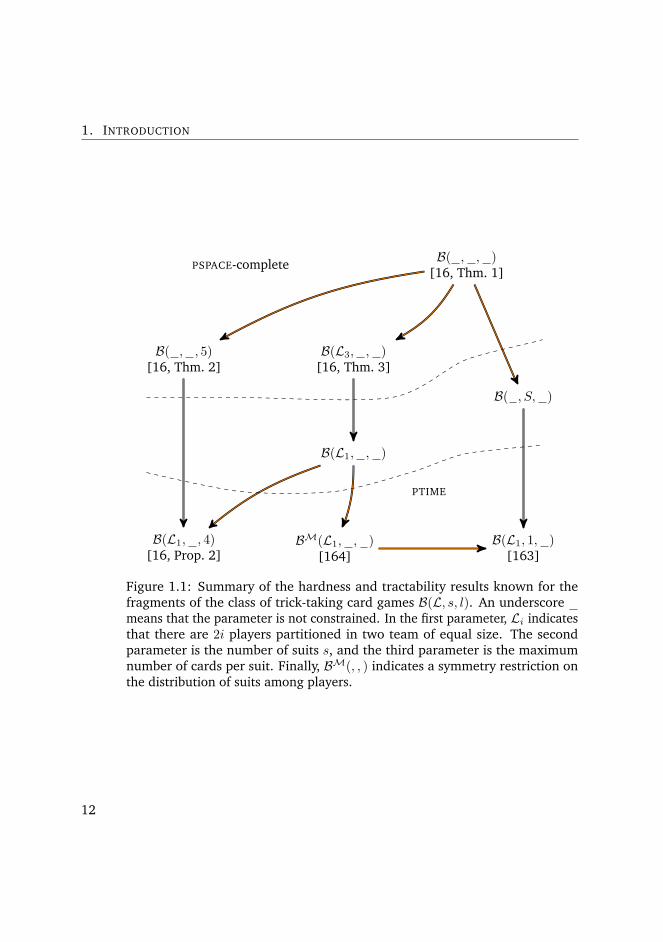
In a recent paper [16], we propose a general model for perfect information
trick-taking card games and prove that solving an instance is PSPACE-complete.
The model can be restricted along many dimensions, including the number of
suits, the number of players, and the number of cards per suit. This allows to
define fragments of the class of trick-taking card games and it makes it possible
to study where the hardness comes from. In particular, tractability results by
Wastlund fall within the framework [163, 164]. We also show that bounding
the number of players or bounding the number of cards per suit is not sufficient
to avoid PSPACE-hardness. The results of the paper can be summed up in the
complexity landscape of Figure 1.1.
[15] Edouard Bonnet, Florian Jamain, and Abdallah Saffidine. Havan-
nah and Twixt are PSPACE-complete. In 8th International Conference on
Computers and Games (CG). Yokohama, Japan, August 2013
[16] Edouard Bonnet, Florian Jamain, and Abdallah Saffidine. On the
complexity of trick-taking card games. In 23rd International Joint Confer-
ence on Artificial Intelligence (IJCAI), Beijing, China, August 2013. AAAI
Press
11
1. INTRODUCTION
B( , , )[16, Thm. 1]
B( , , 5)[16, Thm. 2]
B(L3, , )[16, Thm. 3]
B( , S, )
B(L1, , 4)[16, Prop. 2]
B(L1, , )
BM(L1, , )[164]
B(L1, 1, )[163]
PTIME
PSPACE-complete
Figure 1.1: Summary of the hardness and tractability results known for thefragments of the class of trick-taking card games B(L, s, l). An underscoremeans that the parameter is not constrained. In the first parameter, Li indicatesthat there are 2i players partitioned in two team of equal size. The secondparameter is the number of suits s, and the third parameter is the maximumnumber of cards per suit. Finally, BM(, , ) indicates a symmetry restriction onthe distribution of suits among players.
12

1.3. Contributions not detailed in this thesis
1.3.5 Computational Social Choice
If studying algorithms that compute Nash equilibria and other solution concepts
in specific situations constitute one end of the multi-agent/algorithmic game
theory spectrum, then computational social choice can be seen as the other
end of the spectrum. In computational social choice, one is indeed interested
in solution concepts in their generality. Typical computational social choice
investigations include the following questions.
• What properties does a particular solution concept have?
• Is there a solution concept satisfying a given list of axiom?
• Is the computation of a given property in a given class of multi-agent
systems tractable?
• Can we define a class of multi-agent systems that could approximate a
given real-life interaction among agents?
• If so, what new solution concepts are relevant in the proposed class and
how do they relate to existing solution concepts in previously defined
classes?
A subfield of computational social choice of special interest to us is that of
elections. Elections occur in multiple real-life situations and insight from social
choice theory can be fruitfully applied to settings as varied as political elections,
deciding which movie a group of friend should watch, or even selecting a subset
of submissions to be presented at a conference. Another setting closer to the
main topic of this thesis can also benefit from social choice insights: ensemble
based decision making [112] has recently been successfully applied to the games
of SHOGI [107] and GO [95] via a majority voting system.
Given a set of candidates and a set of voters, a preference profile is a
mapping from each voter to a linear order on the candidates. A voting rule maps
a preference profile to an elected candidate. It is also possible to define voting
rules that map preference profiles to sets of elected candidates. Social choice
theorist study abstract properties of voting rules to understand which rule is
more appropriate to which situation. We refer to Moulin’s book for a detailed
treatment of the field [99].
13
1. INTRODUCTION
An very important solution concept in single winner elections is that of
a Condorcet winner. A Condorcet winner is a candidate that is preferred by
majority of voters to every other candidates in one-to-one elections. A Condorcet
winner does not always exists for a given preference profile, but when one does,
it is reasonable to expect that it should be elected. We proposed a generalization
of the Condorcet winner principle to multiple winner elections [43]. We say that
a set of candidates is a Condorcet winning set if no other candidate is preferred
to all candidates in the set by a majority of voter. Just as Condorcet winners,
Condorcet winning sets satisfy a number of desirable social choice properties.
Just as Condorcet winners, Condorcet winning sets of size 2 are not guaranteed
to exist and we ask whether for any size k, there exists a profile Pk such that Pk
does not admit any Condorcet winning set of size k.
Another line of work that we have started exploring deals with voters’
knowledge of the profile [160]. The fact that voters may or may not know each
other’s linear order on the candidate has multiple consequences, for instance
on the possibilities of manipulation. We propose a model based on epistemic
logic that accounts for uncertainty that voters may have about the profile. This
model makes it possible to model higher-order knowledge, e.g., we can model
that a voter v1 does not know the preference of another voter v3, but that v1knows that yet another voter v2 knows v3’s linear order.
[43] Edith Elkind, Jerome Lang, and Abdallah Saffidine. Choosing col-
lectively optimal sets of alternatives based on the Condorcet criterion.
In Toby Walsh, editor, 22nd International Joint Conference on Artificial
Intelligence (IJCAI), pages 186–191, Barcelona, Spain, July 2011. AAAI
Press. ISBN 978-1-57735-516-8
[160] Hans van Ditmarsch, Jerome Lang, and Abdallah Saffidine. Strategic
voting and the logic of knowledge. In Burkhard C. Schipper, editor, 14th
conference on Theoretical Aspects of Rationality and Knowledge (TARK),
pages 196–205, Chennai, India, January 2013. ISBN 978-0-615-74716-3
1.4 Basic Notions and Notations
We now introduce a few definitions and notations that we will use throughout
the thesis.
14
1.4. Basic Notions and Notations
Definition 1. A transition system T is a tuple 〈S,R,−→, L, λ〉 such that
• S is a set of states;
• R is a set of transition labels;
• −→⊆ S ×R× S is a transition relation;
• L is a set of state labels;
• λ : S → 2L is a labeling function. This function associate a set of labels to
each state.
For two states s, s′ ∈ S and a transition label a ∈ R, we write sa−→ s′ instead
of (s, a, s′) ∈−→. If s is a bound state variable, we indulge in writing ∃s a−→ s′
instead of ∃s′ ∈ S, s a−→ s′. Similarly, if s′ is bound, the same notation ∃s a−→ s′
means ∃s ∈ S, s a−→ s′. In the same way, we allow the shortcut ∀s a−→ s′.
We recall that multisets are a generalization of sets where elements are
allowed to appear multiple times. If A is a set, then 2A denotes the power set of
A, that is, the set of all sets made with elements taken from A. Let NA denote
the set of multisets of A, that is, the set of all multisets made with elements
taken from A. We denote the carrier of a multiset M by M∗, that is M∗ is the
set of all elements appearing in M .
We recall that a total preorder on a set is a total, reflexive, and transitive
binary relation. Let A be a set and 4 a total preorder on A. 4 is total so every
pair of elements are in relation: ∀a, b ∈ A we have a 4 b or b 4 a. 4 is reflexive
so every element is in relation with itself: ∀a ∈ A we have a 4 a. 4 is transitive
so ∀a, b, c ∈ A we have a 4 b and b 4 c implies a 4 c.
Basically, a total preorder can be seen as a total order relation where distinct
elements can be on the “same level”. It is possible to have a 6= b, a 4 b, and
b 4 a at the same time.
We extend the notation to allow comparing sets. If 4 is a total preorder on A
and A1 and A2 are two subsets of A, we write A1 4 A2 when ∀a1 ∈ A1, ∀a2 ∈A2, a1 4 a2.
We also extend the notation to have a strict preorder: a ≺ b if and only if
a 4 b and b 64 a. Finally, we extend the strict notation to allow comparing sets,
we write A1 ≺ A2 when ∀a1 ∈ A1, ∀a2 ∈ A2, a1 ≺ a2.
15


2 Two-Outcome Games
We define a formal model of deterministic two-player perfect infor-
mation two-outcome games. We develop a generic best-first-search
framework for such two-outcome games and prove several properties
of this class of best-first-search algorithms. The properties that we ob-
tain include correctness, progression, and completeness in finite acyclic
games. We show that multiple standard algorithms fall within the
framework, including PNS, MCTS, and PP.
The Chapter includes results from the following paper.
[124] Abdallah Saffidine and Tristan Cazenave. Developments on
product propagation. In 8th International Conference on Computers
and Games (CG). Yokohama, Japan, August 2013
Contents
2.1 Game Model . . . . . . . . . . . . . . . . . . . . . . . . . . 18
2.2 Depth First Search . . . . . . . . . . . . . . . . . . . . . . . 23
2.3 Best First Search . . . . . . . . . . . . . . . . . . . . . . . . 26
2.3.1 Formal definitions . . . . . . . . . . . . . . . . . . . 26
2.3.2 Algorithmic description . . . . . . . . . . . . . . . . 28
2.3.3 Properties . . . . . . . . . . . . . . . . . . . . . . . 30
2.4 Proof Number Search . . . . . . . . . . . . . . . . . . . . . 31
2.4.1 The Proof Number Search Best First Scheme . . . . 32
2.5 Monte Carlo Tree Search . . . . . . . . . . . . . . . . . . . . 34
2.6 Product Propagation . . . . . . . . . . . . . . . . . . . . . . 36
2.6.1 Experimental Results . . . . . . . . . . . . . . . . . 38
2.6.2 Results on the game of Y . . . . . . . . . . . . . . . 38
17

2. TWO-OUTCOME GAMES
2.6.3 Results on DOMINEERING . . . . . . . . . . . . . . . 40
2.6.4 Results on NOGO . . . . . . . . . . . . . . . . . . . . 42
2.6.5 Conclusion . . . . . . . . . . . . . . . . . . . . . . . 43
2.1 Game Model
We base the definition of two-outcome games on that of transition system (see
Definition 1). Transition labels are interpreted as agents or players.
Definition 2. A two-outcome game is a transition system 〈S,R,−→, L, λ〉 where
the following restriction holds.
• There are two distinguished agents Max ∈ R and Min ∈ R
• State turns are exclusive: ¬∃s1, s2, s3 ∈ S, s1 Max−−→ s2 ∧ s1 Min−−→ s3.
• There is a distinguished label: Win ∈ L;
We define the max states A and the min states B as the sets of states that
allow respectively Max and Min transitions: A = {s ∈ S, ∃s′ ∈ S, s Max−−→ s′} and
B = {s ∈ S, ∃s′ ∈ S, s Min−−→ s′}.We say that a state is final if it allows no transition for Max nor Min. We
denote the set of final states by F . F = S \ (A ∪ B). States that are not final
are called internal. For two states s1, s2 ∈ S, we say that s2 is a successor of s1if it can be reached by a Max or a Min transition. Formally, we write s1 −→ s2
when s1Max−−→ s2 ∨ s1 Min−−→ s2.
Remark 1. From the turn exclusivity assumption, we derive that A, B, and F
constitute a partition of S.
We say that a state is won, if it is final and it is labelled as a Win: s ∈F ∧Win ∈ λ(s). We say that a state is lost if it is final and it is not won.
Note that we have not mentionned any other agent beside Max and Min nor
any state label besides Win. Other agents and other state labels will have no
influence in this Chapter and we will assume without loss of generality that
R = {Max,Min} and L = {Win}.
18

2.1. Game Model
The game graph is a Direct Acyclic Graph (DAG) if there are no sequences
s0 −→ s1 −→ . . . −→ sk −→ s0. When the game graph is a finite DAG, we can define
the height h of a state to be the maximal distance from that state to a final state.
If s ∈ F then h(s) = 0 and if s ∈ A ∪B then h(s) = 1 +maxs−→s′ h(s′).
Definition 3. A weak Max-solution to a two-outcome game is a subset of states
Σ ⊆ S such that
If s ∈ F then s ∈ Σ⇒ Win ∈ λ(s) (2.1)
If s ∈ A then s ∈ Σ⇒ ∃s Max−−→ s′, s′ ∈ Σ (2.2)
If s ∈ B then s ∈ Σ⇒ ∀s Min−−→ s′, s′ ∈ Σ (2.3)
Conversely, a weak Min-solution is a subset of states Σ ⊆ S such that
If s ∈ F then s ∈ Σ⇒ Win /∈ λ(s) (2.4)
If s ∈ A then s ∈ Σ⇒ ∀s Max−−→ s′, s′ ∈ Σ (2.5)
If s ∈ B then s ∈ Σ⇒ ∃s Min−−→ s′, s′ ∈ Σ (2.6)
Remark 2. Weak Max-solutions on the one hand, and weak Min-solutions on the
other hand are closed under union but are not closed under intersection.
The class of systems that we focus on in this Chapter and in Chapter 3 are
called zero-sum games. It means that the goals of the two players are literally
opposed. A possible understanding of the zero-sum concept in the proposed
formalism for two-outcome games is that each state is either part of some weak
Max-solution, or part of some weak Min-solution, but not both.
Proposition 1. Let Σ be a weak Max-solution and Σ′ be a weak Min-solution. If
the game graph is a finite DAG, then these solutions do not intersect: Σ ∩ Σ′ = ∅.
Proof. Since the game graph is a finite DAG, the height of states is well defined.
We prove the proposition by induction on the height of states.
Base case: if a state s has height h(s) = 0, then it is a final state. If it is part
of the Max-solution, s ∈ Σ, then we know it has label Win, Win ∈ λ(s) and it
cannot be in the weak Min-solution.
Induction case: assume there is no state of height less or equal to n in Σ∩Σ′
and obtain there no state of height n + 1 in Σ ∩ Σ′. Let us take s ∈ Σ such
19

2. TWO-OUTCOME GAMES
that h(s) = n+ 1 and prove that s /∈ Σ′. If s ∈ A then by definition of a weak
Max-solution s has a successor c ∈ Σ. Since all successors of s have height
less or equal to n, we know that h(c) ≤ n. From the induction hypothesis, we
obtain that c is not in Σ′. Hence, s cannot be in Σ′ either as it would require all
successors and c in particular to be in Σ′.
Proposition 2. Let s be a state, if the game graph is a finite DAG, then s belongs
to a weak solution.
Proof. Since the game graph is a finite DAG, the height of states is well defined.
We prove the proposition by induction on the height of states.
Base case: if a state s has height h(s) = 0, then it is a final state. If it has
label Win, then we known s is part of a Max-solution, for instance Σ = {s}.Otherwise, it is part of a Min-solution, for instance Σ = {s}.
Induction case: assume all states of height less or equal to n are part of a
weak solution and obtain that any state of height n+1 is part of a weak solution.
Let us take s ∈ A such that h(s) = n+ 1. Since all successors of s have height
less or equal to n, we know that they are all part of a weak solution. If one
of them is part of weak Max-solution Σ, then Σ ∪ {s} is a weak Max-solution
that contains s. Otherwise, each successor s′ is part of a weak Min-solution
Σs′ . Since weak Min-solutions are closed under union, we can take the union of
these Min-solutions and obtain a Min-solution: Σ =⋃
s−→s′ Σs′ . It is easy to see
that Σ ∪ {s} is a weak Min-solution that contains s.
The same idea works if we take s ∈ B instead, and we omit the details.
Definition 4. A strong solution to a two-outcome game is a partition of S,
(Σ, S \ Σ) such that
If s ∈ F then s ∈ Σ⇔ Win ∈ λ(s) (2.7)
If s ∈ A then s ∈ Σ⇔ ∃s Max−−→ s′, s′ ∈ Σ (2.8)
If s ∈ B then s ∈ Σ⇔ ∀s Min−−→ s′, s′ ∈ Σ (2.9)
Proposition 1 and Proposition 2 directly lead to the following caracterisation
of strong solutions.
Theorem 1 (Existence and unicity of a strong solution). If the game graph is a
finite DAG, then a unique strong solution exists and can be constructed by taking Σ
20

2.1. Game Model
to be the states that are part of some weak Max-solution and S \Σ to be the states
that are part of some weak Min-solution.
Remark 3. A strong solution is a pair of weak solutions that are maximal for the
inclusion relation.
From now on, we will extend the notion of won and lost states to non-final
states by saying that a state is won if it is part of a weak Max-solution and that
it is lost if it is part a weak Min-solution.
It is now possible to give a formal meaning to Allis’s notion of solving a
game ultra-weakly, weakly, and strongly [3, 156].
Remark 4. A game with a specified initial state s0 is ultra-weakly solved when
we have determined whether s0 was won or s0 was lost.
A game with a specified initial state s0 is weakly solved when we have exhibited
a weak solution that contains s0.
A game is strongly solved when we have exhibited a strong solution.
While the finite DAG assumption in the previous statements might seem
quite restrictive, it is the simplest hypothesis that leads to well-definedness and
exclusion of won and lost values for non terminal states. Indeed, if the game
graph allows cycles or if is not finite, then Theorem 1 might not hold anymore.
Example 1. Consider the game G1 = 〈S1, R,−→1, L, λ1〉 with 4 states, S1 =
{s1, s2}, and a cyclic transition relation −→1. The transition relation is defined
extensively as s0Max−−→1 s1, s0
Max−−→1 s2, s1Min−−→1 s0, and s1
Min−−→1 s3. The only
final state to be labelled Win is s3. A graphical representation of G1 is presented
in Figure 2.1a.
G1 admits two strong solutions, ({s0, s1, s3}, {s2}) and ({s3}, {s0, s1, s2}).While s3 is undeniably a win state and s2 is undeniably a lost state, s0 and s1could be considered both at the same time.
Example 2. Consider the game G2 = 〈S2, R,−→2, L, λ2〉 defined so that there
are infinitely many states, S2 = {si, i ∈ N}, and the transition relation −→2 is
such that s2iMax−−→ s2i+1 and s2i+1
Min−−→ s2i+2. λ2 is set so that no states are
labelled Win. A graphical representation of G2 is presented in Figure 2.1b.
G2 admits two strong solutions, (S2, ∅) and (∅, S2). Put another way, we can
consider that all the states are winning or that all the states are losing.
21

2. TWO-OUTCOME GAMES
s0 s1
s2 s3
Max
MinMax Min
(a) Cyclic game graph
max min lost won
s0 s1 s2 . . .
Max Min
(b) Infinite game graph
Figure 2.1: Examples of two-outcome games in which the conclusions of Theo-rem 1 do not apply.
In practice, the vast majority of games actually satisfy this hypothesis. Take
CHESS, for instance, while it is usually possible from a state s to reach after a
couple moves a state s′ where the pieces are set in the same way as in s, s and s′
are actually different. If the sequence of moves that lead from s to s′ is repeated
in s′ we reach yet another state s′′ with the same piece setting. However, s′′ is a
final state because of the threefold repetition rule whereas s and s′ were internal
states. As a consequence, s′ is a different state than s since the aformentionned
sequence of moves does not have the same effect. Therefore, in such a modeling
of CHESS, the game graph is acyclic. The 50-moves rule, acyclicity, and the
fact that there finitely many piece settings ensure that there are finitely many
different states.
Another modeling of CHESS only encodes the piece setting into the state and
relies on the history of reached position to determine values for position. While
introducing dependency on the history is not necessary to define CHESS and
gives rise to a complicated model in which very few formal results have been
established, it is popular among game programmers and researchers as it allows
a representation with fewer distinct states.
The ancient game of GO takes an alternative approach to deal with short
loops in the piece setting graph. The Ko rule makes it illegal to play a move in
a position s that would lead to the same piece setting as the predecessor of s.
This rule makes it necessary to take into account short term history. Observe
that the Ko rule does not prevent cycles of length greater than two in the piece
22
2.2. Depth First Search
setting graph. Another rule called superko rule makes such cycles illegal, but
the superko rule has only been adopted by Chinese, America, and New Zealand
GO federation. On the other hand, Japanese and Korean rules allow long cycles
in the piece setting graph. As a consequence, the game can theoretically last for
an infinite number of moves without ever reaching a final position. In practice,
when a long cycle occurs in Japanese and Korean professionnal play, the two
players can agree to stop the game. This is not understood as a draw as it
would be in CHESS, but is rather seen as a no result outcome and the players are
required to play a new game to determie a winner.
In the rest of this Chapter, we will mostly be concerned with providing
search algorithms for weakly solving games that have a finite game graph with
a DAG structure.
2.2 Depth First Search
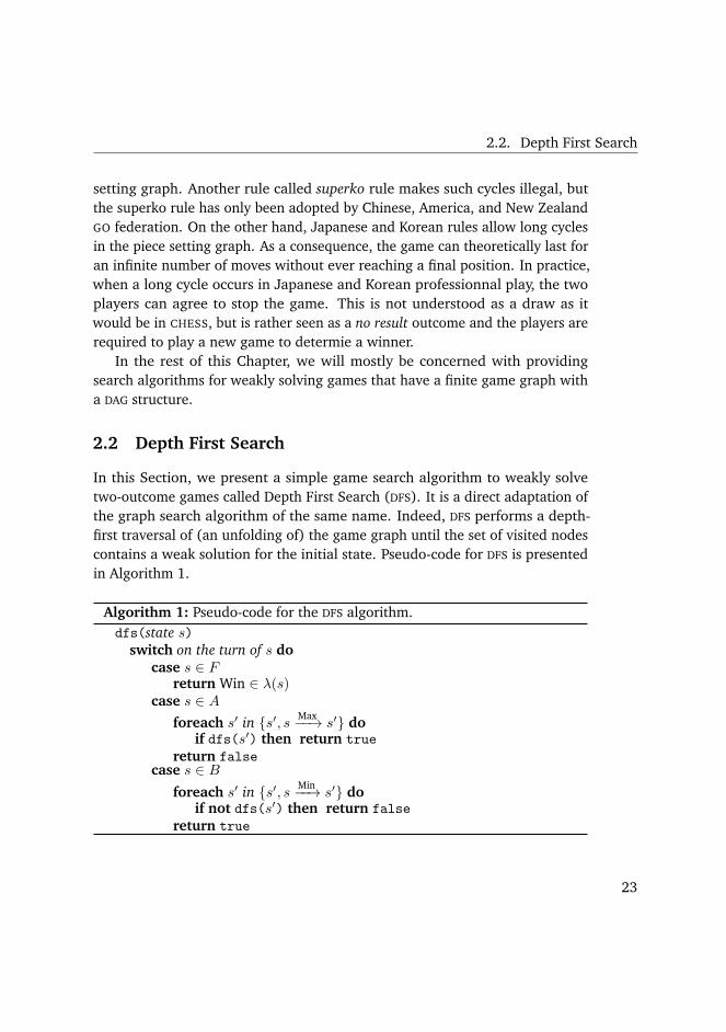
In this Section, we present a simple game search algorithm to weakly solve
two-outcome games called Depth First Search (DFS). It is a direct adaptation of
the graph search algorithm of the same name. Indeed, DFS performs a depth-
first traversal of (an unfolding of) the game graph until the set of visited nodes
contains a weak solution for the initial state. Pseudo-code for DFS is presented
in Algorithm 1.
Algorithm 1: Pseudo-code for the DFS algorithm.
dfs(state s)switch on the turn of s do
case s ∈ Freturn Win ∈ λ(s)
case s ∈ Aforeach s′ in {s′, s Max−−→ s′} do
if dfs(s′) then return true
return falsecase s ∈ B
foreach s′ in {s′, s Min−−→ s′} doif not dfs(s′) then return false
return true
23
2. TWO-OUTCOME GAMES
Remark 5. The specification of DFS in Algorithm 1 is non-deterministic. One
consequence of this non-determinism is that the algorithm might or might not
converge for a given game. This will be expanded upon in Example 3.
If the game graph is a finite DAG, then its unfolding is a finite tree. The DFS
algorithm visits each state of the unfolded tree at most once so it can only visit
a finite number of states in the unfolding. This is summed up in Proposition 3.
Proposition 3 (Termination). If the game graph is a finite DAG, then the DFS
algorithm terminates.
Proof. If the game graph is a finite DAG, then the height of states is well-defined.
We prove the proposition by induction on the height of the argument state s.
Base case: h(s) = 0. When s is a final state, DFS returns without performing
a recursive call.
Induction case: Assume DFS terminates whenever given an argument of
height less or equal to n and prove that it terminates when given an argument s
of height n+ 1. Let s be a state of height n+ 1. s is either a max state or a min
state, and all its successors have height less or equal to n. Since the game graph
is finite, we know that s only has finitely many successors. We conclude that
when DFS is called with s as argument, finitely many recursive calls to DFS are
performed and so the algorithm terminates.
The DFS algorithm is correct, that is, if dfs(s) terminates, then it returns
true only when there exists a weak Max-solution containing s, and it returns
false only when there exists a weak Min solution containing s.
Proposition 4 (Correctness). If DFS returns true when given argument s, then
there exists a weak Max-solution including s. If it returns false then there is a
weak Min-solution including s.
Proof. Induction on the depth of the call-graph of DFS.
This property establised by Proposition 4 does not rely on the finite DAG
assumption. However, if we make the finite DAG assumption, then Proposition 3
and 4 combine and lead to the following completeness result.
24

2.2. Depth First Search
s0
s1
s2
s3
s4
s5
s6
s7
Max
Max
Min
Min
Min
Max
Max
Max
Max
Figure 2.2: Example of a two-outcome game in which the DFS algorithm mightor might not terminate. s6 is a lost final node and s7 is a won final node.
Theorem 2 (Completeness in finite DAG). When called on a state s of a game
which graph is a finite DAG, then DFS terminates and returns true exactly when s
is won and returns false exactly when s is lost.
If the game graph is allowed to be infinite or to contain cycles, then DFS
might or might not terminate.
Example 3. Consider the game presented in Figure 2.2. The graph of the
game presents a cycle, {s1, s3}, and the game indeed has two strong solutions,
({s0, s1, s2, s3, s4, s5, s7}, {s6}) and ({s0, s2, s4, s5, s7}, {s1, s3, s6}). s0 is part of
the Max weak-solution of every strong solution, so it can be considered as a
won state. Still, it is possible that a call to DFS with s0 as argument does not
terminate and it is also possible that it terminates and returns true. Indeed, s0has two successor states, s1 and s2, and DFS is called recursively in either of the
two non-deterministically. On the one hand, if the first recursive call from s0takes s1 as argument, then the algorithm gets stuck in an infinite loop. On the
other hand, if the first recursive call from s0 takes s2 as argument, then that
calls returns true and the loop is shortcut without calling DFS on s1.
25
2. TWO-OUTCOME GAMES
2.3 Best First Search
We propose in this section a generic Best First Search (BFS) framework. The
framework can be seen as a template that makes it easy to define game tree
search algorithms for two-outcome games. The framework is general enough to
encompass PNS and MCTS in particular.
2.3.1 Formal definitions
Definition 5. An information scheme is a tuple 〈V,⊤,⊥,4, H〉 such that V is a
set of information values; ⊤ ⊂ V and ⊥ ⊂ V are two distinguished sets of top
values and bottom values.
4 is a selection relation parameterized by a player and an information
context: ∀v ∈ V we have 4vmax and 4v
min two total preorders on V .
H is an update function parameterized by a player. It aggregates multiple
pieces of information into a single information value. Since we allow pieces of
information to be repeated, we need to use multisets rather than sets. We have
Hmax : NV → V and Hmin : NV → V .
This set represents the information that can be associated to nodes of the
tree. The intended interpretation of v1 4vp v2 is that v2 is preferred to v1 by
player p under context v.
We extend the notation for the selection relation as follows: v1 4p v2 is
short for ∀v ∈ V, v1 4vp v2. It is not hard to see that 4p is also a total preorder.
Definition 6. We define the set of solved values as S = ⊤ ∪ ⊥ and the set of
unsolved values as U = V \ S.
Example 4. Let the set of information values be the real numbers with both
infinites: V = R ∪ {−∞,+∞}, the bottom values be the singleton ⊥ = {−∞},and the top values be ⊤ = {+∞}. We can define a selection relation 4 that
is independent of the context as ∀x ∈ V , a 4xMax b iff a ≤ b and a 4x
Min b iff
a ≥ b. Finally, we can take for the update function the standard max and min
operators: HMax = max and HMin = min. Together, these elements make an
information scheme: MinMaxISdef= 〈V,⊤,⊥,4, H〉.
The set of solved values is S = {−∞,+∞} and the set of unsolved values is
U = R.
26
2.3. Best First Search
Definition 7. An information scheme 〈V,⊤,⊥,4, H〉 is well formed if the fol-
lowing requirements are met. The top and bottom values do not overlap.
⊤ ∩⊥ = ∅ (2.10)
The selection relation avoids lost values for max and avoid won values for min.
⊥ ≺max V \ ⊥ and ⊤ ≺min V \ ⊤ (2.11)
A top value is sufficient to allow a top max update. A multiset with only bottom
values leads to a bottom max update.
M∗ ∩ ⊤ 6= ∅ implies Hmax(M) ∈ ⊤M∗ ⊆ ⊥ implies Hmax(M) ∈ ⊥
(2.12)
A bottom value is sufficient to allow a bottom min update. A multiset with only
top values leads to a top min update.
M∗ ∩ ⊥ 6= ∅ implies Hmin(M) ∈ ⊥M∗ ⊆ ⊤ implies Hmin(M) ∈ ⊤
(2.13)
An update cannot create top and bottom values without justification.
M∗ ∩ S = ∅ implies Hp(M) /∈ S (2.14)
Proposition 5. The information scheme defined in Example 4 is well formed.
We will only be interested in well-formed information scheme.
Definition 8. Let G = 〈S,R,−→, L, λ〉 be a two-outcome game, and let I =
〈V,⊤,⊥,4, H〉 be a well-formed information scheme, and ζ be an information
function ζ : S → V . Then 〈G, I, ζ〉 is a best first scheme if the following two
constraints are met.
• The information function needs to be consistent. If a state s is associated
to a top value ζ(s) ∈ ⊤ then there exists a weak Max-solution containing
s. Conversely, if a state s is associated to a bottom value ζ(s) ∈ ⊥ then
there exists a weak Min-solution containing s.
27
2. TWO-OUTCOME GAMES
• The information function needs to be informative. If a state is final, then
it is associated to a solved value by the information function. s ∈ F ⇒ζ(s) ∈ S.
While the consistency requirement might seem daunting at first, there are
multiple ways to create information function that are consistent by construction.
For instance, any function returning a top or a bottom value when and only
when the argument state is final is consistent.
2.3.2 Algorithmic description
We now show how we can construct a best first search algorithm based on a
best first scheme as defined in Definition 8. The basic idea is to progressively
build a tree in memory and to associate an information value and a game state
to each node of the tree until a weak solution can be derived from the tree.
We assume that each node n of the tree gives access to the following fields.
n.info ∈ V is the information value associated to the node. n.state ∈ S is the
state associated to the node. If n is not a leaf, then n.chidren is the set of
children of n. If n is not the root node, then n.parent is the parent node of n.
We allow comparing nodes directly based on the selection relation 4: for any
two nodes n1 and n2, we have n1 4vp n2 iff n1.info 4v
p n2.info. We also indulge
in applying the update function to nodes rather than to the corresponding
information value: if C is a set of nodes and M is the corresponding multiset of
information values, M = {n.info, n ∈ C}, then H(C) is short for H(M).
Algorithm 2 develops an exploration tree for a given state s. To be able
to orient the search efficiently towards proving a win or a loss for player Max
instead of just exploring, we need to attach additional information to the nodes
beyond their state label.
If the root node is not solved, then more information needs to be added to
the tree. Therefore a (non-terminal) leaf needs to be expanded. To select it, the
tree is recursively descended selecting at each node the next child according to
the 4 relation.
Once the node to be expanded, n, is reached, each of its children are added
to the tree and they are evaluated with ζ. Thus the status of n changes from
leaf to internal node and its value has to be updated with the H function. This
update may in turn lead to an update of the value of its ancestors.
28

2.3. Best First Search
After the values of the nodes along the descent path are updated, another
leaf can be expanded. The process continues iteratively with a descent of the
tree, its expansion and the consecutive update until the root node is solved.
Algorithm 2: Generic pseudo-code for a best-first search algorithm intwo-player games.
extend(node n)foreach s′ in {s′, n.state→ s′} do
new node n′
n′.state← s′ ; n′.info← ζ(s′)Add n′ to n.children
backpropagate(node n)old info← n.infoswitch on the turn of n.state do
case n.state ∈ A n.info← Hmax(n.children)case n.state ∈ B n.info← Hmin(n.children)
if old info = n.info ∨ n = r then return nelse return backpropagate(n.parent)
bfs(state s)new node rr.state← s ; r.info← ζ(s)n← rwhile r.info /∈ S do
while n is not a leaf doC ← n.childrenswitch on the turn of n.state do
case n.state ∈ A n← any element ∈ C maximizing 4n.infomax
case n.state ∈ B n← any element ∈ C maximizing 4n.infomin
extend(n)n← backpropagate(n)
return r
29

2. TWO-OUTCOME GAMES
2.3.3 Properties
We turn on to proving a few properties of BFS algorithms generated with the
proposed framework. That is, we assume given a blabla and we prove formal
properties on this system. Thus any best first scheme constructed with this
framework will satisfy the properties presented in this section. The typical
application of this work is to alleviate the proof burden of the algorithm designer
as it is now sufficient to show that a new system is actually a best first scheme.
Proposition 6 (Correctness). If n.info ∈ ⊤ then n.state is contained in a weak
Max-solution. Conversely if n.info ∈ ⊥ then n.state is contained in a weak Min-
solution.
Proof. Structural induction on the current tree using the consistency of the
evaluation function.
Proposition 7. If n is a node reached by the BFS algorithm during the descent,
then it is not solved yet: n.info /∈ S.
Proof. Proof by induction.
Base case: When n is the root of the tree, n = r, we have r.info /∈ S by
hypothesis.
Induction case: assume n is a child node of p, p.info /∈ S, and n maximizes
the selection relation. Let M = {n′.info for n′ ∈ p.children}. If p is a Max state,
p.state ∈ A, we note that p.info = Hmax(M).
Given that p is not solved, we have in particular that p.info /∈ ⊥ and therefore
M∗ 6⊆ ⊥ from Equation (2.12). As a result, at least one element in M does not
belong to ⊥. Let n′ be a node such that n′.info /∈ ⊥. n maximizes 4max so n′ is
not strictly preferred to n. Since 4max avoids lost values and n′.info is not lost,
then we know that n cannot be lost either (Equation (2.11)). Thus, n.info /∈ ⊥.
We also have that p.info /∈ ⊤ and therefore M∗ ∩ ⊤ = ∅ from Equation
(2.12). As a result, no element in M belongs to ⊤. In particular, n.info /∈ ⊤ and
so we conclude that n is not be solved: n.info /∈ S.
The case where p is a Min state is similar and is omitted.
Proposition 8 (Progression). If n is a leaf node reached by the BFS algorithm
during the descent, then the corresponding position is not final: n.state /∈ F .
30
2.4. Proof Number Search
Proof. We have assumed in Definition 8 that the evaluation function ζ was in-
formative. That is, n.state ∈ F implies n.info ∈ S. We know from Proposition 7
that n.info /∈ S. Hence, we can conclude that n.state /∈ F .
The direct consequence of Proposition 8 is that the extend() procedure
always add at least one node to the tree. Therefore, the size of the tree grows
after each iteration.
Proposition 9 (Convergence in finite games). If the game graph is finite and
acyclic, the BFS algorithm terminates.
We will see in Section 2.4, 2.5, and 2.6 a few classical algorithms can be
expressed the suggested formalism and inherit its theoretical properties. Many
more are possible, for instance the results we obtain also apply to the best first
scheme derived from Example 4 .
2.4 Proof Number Search
PNS [4, 74] is a best first search algorithm that enables to dynamically focus
the search on the parts of the search tree that seem to be easier to solve. PNS
based algorithms have been successfully used in many games and especially as
a solver for difficult games such as CHECKERS [137], SHOGI [141], and GO [73].
There has been a lot of developments of the original PNS algorithm [4].
An important problem related to PNS is memory consumption as the tree has
to be kept in memory. In order to alleviate this problem, V. Allis proposed
PN2 [3]. It consists in using a secondary PNS at the leaves of the principal PNS.
It allows to have much more information than the original PNS for equivalent
memory, but costs more computation time. PN2 has recently been used to solve
FANORONA [131].
The main alternative to PN2 is the DFPN algorithm [103]. DFPN is a depth-first
variant of PNS based on the iterative deepening idea. DFPN will explore the game
tree in the same order as PNS with a lower memory footprint but at the cost of
re-expanding some nodes.
We call effort numbers heuristic numbers which try to quantify the amount
of information needed to prove some fact about the value of a position. The
higher the number, the larger the missing piece of information needed to prove
31

2. TWO-OUTCOME GAMES
the result. When an effort number reaches 0, then the corresponding fact has
been proved to be true, while if it reaches∞ then the corresponding fact has
been proved to be false.
In PNS we try to decide whether a node belongs to a weak Max-solution.
That is, we simultaneously try to find a weak Max-solution containing it and
to prove that it does not belongs to any weak Max-solution. We will use the
standard PNS terminology for the remaining of this Section, that is, we say that
we prove a node when we find a weak Max-solution containing it, and that we
disprove a node when we find a weak Min-solution containing it.
2.4.1 The Proof Number Search Best First Scheme
We use N∗ to denote the set of positive integers: N∗ = {1, 2, . . .}.
The information value associated to nodes contains two parts: we have
v = (p, d) with p, d ∈ N ∪ {∞}. The proof number (p) represents an estimation
of the remaining effort needed to prove the node, while the disproof number (d)
represents an estimation of the remaining effort needed to disprove the node.
When Max solution has been found we have p(n) = 0 and d(n) =∞, and when
a Min solution has been found we have p(n) =∞ and d(n) = 0.
V = N∗ × N
∗ ∪ {(0,∞), (∞, 0)}⊤ = {(0,∞)} and ⊥ = {(∞, 0)}
(2.15)
The basic idea in PNS is to strive for proofs that seem to be easier to obtain.
Thus, we define the selection relation so that if Max is on turn, then the selected
child minimizes the proof number and if Min is on turn, the selected child
minimizes the disproof number.
(p, d) 4max (p′, d′) iff p′ ≤ p(p, d) 4min (p′, d′) iff d′ ≤ d
(2.16)
If an internal node n corresponds to a Max position, then proving one child
of n is sufficient to prove n and disproving n requires disproving all its children.
As a consequence, the (greatest lower bound on the) amount of effort needed
to prove n is the amount of effort needed for the easiest child of n to be proved,
and the amount of effort needed to prove n is bounded below by the sum of
32

2.4. Proof Number Search
efforts for all children of n. A similar intuition for Min nodes leads to the update
functions.
Hmax(M) =
min(p,d)∈M
p,∑
(p,d)∈M
d
Hmin(M) =
∑
(p,d)∈M
p, min(p,d)∈M
d
(2.17)
It is not hard to see that for any multiset of V , M , we have HMax(M) ∈ Vand HMin(M) ∈ V . Therefore we have an information scheme.
Proposition 10. The information scheme is well-formed.
The evaluation function, also known as the initialization function in the PNS
litterature, is a simple admissible bound on the effort to prove or disprove a
node. If the node corresponds to a final position, then we know its value. If
it is a Win, the remaining effort need to prove it is p = 0 and the remaining
effort to disprove it can be set to d =∞ since we know this node cannot ever
be disproved. Conversely, if the final node is not a Win then we set the proof
number to∞ and the disproof number to 0.
If the node n corresponds to a non-final position, then (dis)proving will
require expanding at least one node (this very node n), so we set p = 1 and
d = 1. This can be summed up with the following initialization formulas.
∀s ∈ A ∪B,ζ(s) = (1, 1)
∀s ∈ F,Win ∈ λ(s)⇒ ζ(s) = (0,∞)
∀s ∈ F,Win /∈ λ(s)⇒ ζ(s) = (∞, 0)(2.18)
ζ is consistent and informative. Therefore, we have a best first scheme. From
Proposition 6 and Proposition 9 we have that PNS is correct, and converges in
finite acyclic games.
Example 5. Here is an example of finite game with a cycle in which PNS does
not converge.
Example 6. Here is an example of an infinite game without cycles in which PNS
does not converge.
33

2. TWO-OUTCOME GAMES
2.5 Monte Carlo Tree Search
MCTS is a very successful algorithm for multiple complete information games
such as GO [40, 41, 54, 86, 114], HEX [25, 7], or LINES OF ACTION [166].
MCTS is a recent game tree search technique based on multi-armed bandit
problems [20]. MCTS has enabled a huge leap forward in the playing level of
artificial GO players. It has been extended to prove wins and losses under the
name MCTS Solver [165, 46]. It is this MCTS Solver algorithm that we describe
here.
The basic idea in MCTS is to evaluate whether a state s is favourable to
Max via Monte Carlo playouts in the tree below s. A Monte Carlo playout is
a random path of the tree below s ending in a terminal state. Performing a
playout and checking the type of the corresponding terminal state can be done
as demonstrated in Algorithm 3.
Monte Carlo programs usually deal with transpositions the simple way: they
do not modify the UCT formula and develop a DAG instead of a tree.
Algorithm 3: Pseudo-code for a Monte Carlo Playout.
playout(state s)switch on the turn of s do
case s ∈ F ∧Win ∈ λ(s) return 1case s ∈ F ∧Win /∈ λ(s) return 0otherwise
s′ ← random state such that s→ s′
return playout(s′)
MCTS explores the Game Automaton (GA) in a best first way by using aggre-
gates of information given by the playouts.
V = N× N∗ × {0, 1, 2}
⊤ = N× N∗ × {2}
⊥ = N× N∗ × {0}
(2.19)
An information value is a triple (r, t, s) where t denotes the total number of
playouts rooted below n and r denotes the number of playouts ending in a Win
state among them.
34

2.5. Monte Carlo Tree Search
We also have the label s that represents the solution status and allows
to avoid solved subtrees. s can take three values: 0, 2, or 1. These values
respectively mean that the corresponding node was weakly Min-solved, weakly
Max-solved, or not solved yet for this node.
(r, t, s) 4(r0,t0,s0)max (r′, t′, s′) iff
s < s′
s = s′ and rt+√
2 ln t0t≤ p′
t′+√
2 ln t0t′
(r, t, s) 4(r0,t0,s0)min (r′, t′, s′) iff
s′ < s
s = s′ and −rt
+√
2 ln t0t≤ −r′
t′+√
2 ln t0t′
(2.20)
When a node is not solved yet, we are faced with an exploration-exploitation
dilemma between running playouts in nodes which have not been explored
much (t is small) and running playouts in nodes which seem successful (high rt
ratio). This concern is addressed using the UCB formula [9, 20].
∀s ∈ A ∪B, ζ(s) = (playout(s), 1, 1)
∀s ∈ F,Win ∈ λ(s)⇒ ζ(s) = (1, 1, 2)
∀s ∈ F,Win /∈ λ(s)⇒ ζ(s) = (0, 1, 0)
(2.21)
To initialize a value corresponding to a non terminal position s we call the
playout(s) procedure (Algorithm 3). If the position s is terminal, then the
initial value depends on whether s is a Win state.
Hmax(M) = (∑
(r,t,s)∈M
r,∑
(r,t,s)∈M
t, max(r,t,s)∈M
s)
Hmin(M) = (∑
(r,t,s)∈M
r,∑
(r,t,s)∈M
t, min(r,t,s)∈M
s)(2.22)
The total number of playouts rooted at a node can be viewed as the sum of
the number of playouts rooted at each child. Similarly, the number of playouts
ending in a Win state is the sum of the corresponding number at each child.
35

2. TWO-OUTCOME GAMES
Proposition 11. ζ is informative and consistent, the information scheme is well-
formed, and so we have a best first scheme.
Remark 6. The evaluation of a leaf node in MCTS as presented in Equation 2.21
takes the form of games played randomly until a terminal position. It can also be
the value of a heuristical evaluation function after a few random moves [92, 166].
We denote the latter variant as MCTS-E.
2.6 Product Propagation
PP is a way to backup probabilistic information in a two-player game tree
search [144]. It has been advocated as an alternative to minimaxing that does
not exhibit the minimax pathology [110, 69, 70].
PP was recently proposed as an algorithm to solve games, combining ideas
from PNS and probabilistic reasoning [146]. In Stern’s paper, PP was found to
be about as performant as PNS for capturing GO problems.
In this Chapter, we express PP as an instance of the BFS framework presented
in Section 2.3 and conduct an extensive experimental study of PP, comparing
it to various other paradigmatic solving algorithms and improving its memory
consumption and its solving time. Doing so, we hope to establish that PP is an
important algorithm for solving games that the game search practician should
know about. Indeed, we exhibit multiple domains in which PP performs better
than the other tested game solving algorithms.
The baseline game tree search algorithms that we use to establish PP’s
value are DFS (see Section 2.2); PNS [4, 155, 74] (see Section 2.4); and MCTS
Solver [165] which was recently used to solve the game of HAVANNAH on size
4 [46] (see Section 2.5).
In PP, each node n is associated to a single number PP called the probability
propagation number for n, such that PP ∈ [0, 1]. The PP of a leaf corresponding
to a Max win is 1 and the PP of a Max loss is 0.
V = [0, 1], ⊤ = {1}, and ⊥ = {0} (2.23)
The probability propagation number of a node n can intuitively be under-
stood as the likelihood of n being a Max win given the partially explored game
tree. With this interpretation in mind, natural update rules can be proposed.
36

2.6. Product Propagation
If n is an internal Min node, then it is a win for Max if and only if all children
are win for Max themselves. Thus, the probability that n is win is the joint
probability that all children are win. If we assume all children are independent,
then we obtain that the PP of n is the product of the PP of the children for Min
nodes. A similar line of reasoning leads to the formula for Max nodes.
Hmax(M) = 1−∏
p∈M
(1− p)
Hmin(M) =∏
p∈M
p(2.24)
To define the PP of a non-terminal leaf l, the simplest is to assume no
information is available and initiate the PP information value to 12 .
∀s ∈ A ∪B, ζ(s) = 0.5
∀s ∈ F,Win ∈ λ(s)⇒ ζ(s) = 1
∀s ∈ F,Win /∈ λ(s)⇒ ζ(s) = 0
(2.25)
Note that this explanation is just a loose interpretation of the probability
propagation numbers and not a formal justification. Indeed, the independence
assumption does not hold in practice, and in concrete games n is either a win
or a loss for Max but it is not a random event. However, this probabilistic
analogy mainly serves as an intuition for the algorithm and it is reasonable not
to feel constrained by the lack of independance as the algorithm performs well
nontheless.
To be able to use the generic BFS framework, we still need to specify which
leaf of the tree is to be expanded. The most straightforward approach is to
select the child maximizing PP when at a Max node, and to select the child
minimizing PP when at a Min node.
p 4max p′ if and only if p ≤ p′
p 4min p′ if and only if p′ ≤ p
(2.26)
Proposition 12. ζ is informative and consistent, the information scheme is well-
formed, and so we have a best first scheme.
Note that it is also possible to use a heuristical evaluation function taking
values in (0, 1) to evaluate leaves.
37
2. TWO-OUTCOME GAMES
2.6.1 Experimental Results
While the performance of PP as a solver has matched that of PNS in GO [146],
it has proven to be disappointing in SHOGI.1 We now exhibit several domains
where the PP search paradigm outperforms more classical algorithms.
In the following sets of experiments, we do not use any domain specific
knowledge besides an evaluation function where appropriate. We are aware
that the use of such techniques would improve the solving ability of all our
programs. Nevertheless, we believe that showing that a generic and non-
optimized implementation of PP performs better than generic and non-optimized
implementations of PNS, MCTS, or DFS in a variety of domains provides good
reason to think that the ideas underlying PP are of importance in game solving.
Besides PP, PNS, MCTS, and DFS, we also try to incorporate transpositions in
PP and PNS [139]. We thus obtain PP with Transpositions (PPT) and PNS with
Transpositions (PNT). Finally, we also adapt the PN2 [19] idea to PP and try
the resulting PP2 algorithm, that is, instead of directly using an heuristical
evaluation function to evaluate leaves that correspond to internal position, we
perform a nested call to PP.
2.6.2 Results on the game of Y
The game of Y was discovered independently by Claude Shannon in the 50s,
and in 1970 by Schensted and Titus. It is played on a triangular board with a
hexagonal paving. Players take turns adding one stone of their color on empty
cells of the board. A player wins when they succeed in connecting all three
edges with a single connected group of stones of their color. Just as HEX, Y
enjoys the no-draw property.
The current best evaluation function for Y is the reduction evaluation func-
tion [162]. This evaluation function naturally takes values in [0, 1] with 0
(resp. 1) corresponding to a Min (resp. Max) win.
PNS with the mobility initialization could not solve any position in less than 3
minutes in a preliminary set of about 50 positions. As a result we did not include
this solver in our experiment with a larger set of positions. The experiments on
Y was carried out as follows. We generated 77, 012 opening positions on a board
1Akihiro Kishimoto, personnal communication.
38

2.6. Product Propagation
Table 2.1: Number of positions solved by each algorithm and number of posi-tions on which each algorithm was performing best.
PP MCTS MCTS-E
Positions solved 77,010 76,434 69,298Solved fastest 68,477 3,645 4,878Fewest iterations 22,621 35,444 18,942
of size 6. We then ran PP using the reduction evaluation function, MCTS using
playouts with a random policy, and a variant of MCTS using the same reduction
evaluation instead of random playouts (MCTS-E). For each solver, we recorded
the total number of positions solved within 60 seconds. Then, for each solving
algorithm, we computed the number of positions among those 77, 012 which
were solved faster by this solver than by the two other solver, as well as the
number of positions which needed fewer iterations of the algorithm to be solved.
The results are presented in Table 2.1.
We see that the PP algorithms was able to solve the highest number of
positions, 77, 010 positions out of 77, 012 could be solved within 60 seconds. We
also note that for a very large proportion of positions (68, 477), PP is the fastest
algorithm. However, MCTS needs fewer iterations than the other two algorithms
on 35, 444 positions. A possible interpretation of these results is that although
iterations of MCTS are a bit more informative than iterations of PP, they take
much longer. As a result, PP is better suited to situations where time is the most
important constraint, while MCTS is more appropriate when memory efficiency
is a bottleneck. Note that if we discard MCTS-E results, then 72, 830 positions are
solved fastest by PP, 4, 180 positions are solved fastest by MCTS, 30, 719 positions
need fewest iterations to be solved by PP, and 46, 291 need fewest iterations by
MCTS.
Figure 2.3 displays some of these results graphically. We sampled about 150
positions of various difficulty from the set of 77, 012 Y positions, and plotted the
time needed to solve such positions by each algorithm against the time needed
by PP. We see that positions that are easy for PP are likely to be easy for both
MCTS solvers, while positions hard for PP are likely to be hard for both other
solvers as well.
39

2. TWO-OUTCOME GAMES
0.1
1
10
0.1 1 10
Tim
e
PP time
PP timeMCTS time
MCTS-E time
Figure 2.3: Time needed to solve various opening positions in the game of Y.
2.6.3 Results on DOMINEERING
DOMINEERING is played on a rectangular board. The first player places a vertical
2× 1 rectangle anywhere on the board. The second player places an horizontal
2× 1 rectangle, and the games continues like that until a player has no legal
moves. The first player that has no legal moves has lost.
DOMINEERING has already been studied in previous work by game search
specialists as well as combinatorial game theorists [18, 82].2 While these
papers focusing on DOMINEERING obtain solution for relatively large boards,
we have kept ourselves to a naive implementation of both the game rules and
the algorithms. In particular, we do not perform any symmetry detection nor
make use of combinatorial game theory techniques such as decomposition into
subgames.
We presents results for the following algorithms: DFS, PNT [139], PN2 [19],
PP, PPT and PP2. The PNS algorithm could not find a single solution within 107
node expansion when transpositions where not detected and it is thus left out.
For PP variants, the probability of a non solved leaf is computed as the
2Some results can also be found on http://www.personeel.unimaas.nl/uiterwijk/
Domineering_results.html.
40
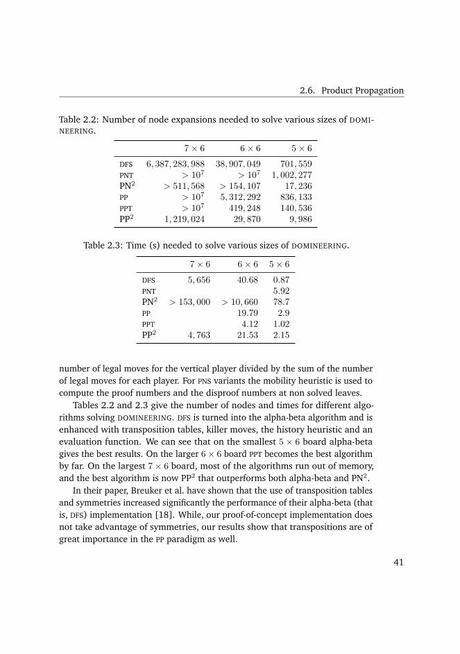
2.6. Product Propagation
Table 2.2: Number of node expansions needed to solve various sizes of DOMI-NEERING.
7× 6 6× 6 5× 6
DFS 6, 387, 283, 988 38, 907, 049 701, 559PNT > 107 > 107 1, 002, 277PN2 > 511, 568 > 154, 107 17, 236PP > 107 5, 312, 292 836, 133PPT > 107 419, 248 140, 536PP2 1, 219, 024 29, 870 9, 986
Table 2.3: Time (s) needed to solve various sizes of DOMINEERING.
7× 6 6× 6 5× 6
DFS 5, 656 40.68 0.87PNT 5.92PN2 > 153, 000 > 10, 660 78.7PP 19.79 2.9PPT 4.12 1.02PP2 4, 763 21.53 2.15
number of legal moves for the vertical player divided by the sum of the number
of legal moves for each player. For PNS variants the mobility heuristic is used to
compute the proof numbers and the disproof numbers at non solved leaves.
Tables 2.2 and 2.3 give the number of nodes and times for different algo-
rithms solving DOMINEERING. DFS is turned into the alpha-beta algorithm and is
enhanced with transposition tables, killer moves, the history heuristic and an
evaluation function. We can see that on the smallest 5 × 6 board alpha-beta
gives the best results. On the larger 6× 6 board PPT becomes the best algorithm
by far. On the largest 7× 6 board, most of the algorithms run out of memory,
and the best algorithm is now PP2 that outperforms both alpha-beta and PN2.
In their paper, Breuker et al. have shown that the use of transposition tables
and symmetries increased significantly the performance of their alpha-beta (that
is, DFS) implementation [18]. While, our proof-of-concept implementation does
not take advantage of symmetries, our results show that transpositions are of
great importance in the PP paradigm as well.
41

2. TWO-OUTCOME GAMES
Table 2.4: Number of node expansions needed to solve various sizes of NOGO.
18× 1 20× 1 22× 1
DFS 4, 444, 384 154, 006, 001 3, 133, 818, 285PNT 2, 015, 179 > 107 > 107
PN2 > 22, 679 > 29, 098PP 1, 675, 159 > 107 > 107
PPT 206, 172 657, 045 4, 853, 527PP2 14, 246
Table 2.5: Time (s) needed to solve various sizes of NOGO.
18× 1 20× 1 22× 1
DFS 10.43 361.0 7, 564PNT 144.2 > 809PN2 > 3, 607 > 4, 583PP 39.96 > 257.0PPT 21.06 85.11 801.0PP2 109.7
2.6.4 Results on NOGO
NOGO is the misere version of the game of GO. It was presented in the BIRS
2011 workshop on combinatorial game theory [28].3 The first player to capture
has lost.
We present results for the following algorithms: DFS, PNT [139], PN2 [19],
PP, PPT and PP2. Again, the PNS algorithm could not find a single solution within
107 node expansion and is left out.
For standard board sizes such as 4 × 4 or 5 × 4, DFS gives the best results
among the algorithms we study in this paper. We have noticed that for N × 1
boards for N > 20, PPT becomes competitive. Results for a few board sizes are
given in Table 2.4 for the number of nodes and in Table 2.5 for the times.
3http://www.birs.ca/events/2011/5-day-workshops/11w5073
42

2.6. Product Propagation
2.6.5 Conclusion
In this Section, we have presented how to define and use Product Propagation
(PP) in order to solve abstract two-player games. We briefly described how to
extend PP so as to handle transpositions and to reduce memory consumption
with the PP2 algorithm. For the three games that have been tested (i.e., Y,
DOMINEERING, and NOGO), we found that our extensions of PP are able to better
solve games than the other solving algorithms.
Being a BFS algorithm, PP is quite related to PNS and MCTS. As such, it seems
natural to try and adapt ideas that proved successful for these algorithms to the
Product Propagation paradigm. For instance, while PNS and PP are originally
designed for two-outcome games, future work could adapt the ideas underlying
MOPNS [123] (see Section 3.7) to turn PP into an algorithm addressing more
general games. Adapting more elaborate schemes for transpositions could also
prove interesting [100, 73, 125].
43


3 Multi-Outcome Games
We define a formal model of deterministic two-player perfect infor-
mation zero-sum games called multi-outcome game. We adapt the
concept of information scheme to multi-outcome game and obtain a
Best First Search (BFS) framework.
We show that a generalization of Monte Carlo Tree Search (MCTS)
Solver, termed Score Bounded Monte Carlo Tree Search (SBMCTS), can
be obtained as an instance of the BFS framework. We then develop a
principled approach to create a multi-outcome information scheme
based on two-outcome information scheme that we call multization.
We use it to derive a new Multiple-Outcome Proof Number Search
(MOPNS) algorithm that generalizes Proof Number Search (PNS) to
multi-outcome games.
The Chapter includes results from the following papers.
[26] Tristan Cazenave and Abdallah Saffidine. Score bounded Monte-
Carlo tree search. In H. van den Herik, Hiroyuki Iida, and Aske Plaat,
editors, Computers and Games, volume 6515 of Lecture Notes in
Computer Science, pages 93–104. Springer-Verlag, Berlin / Heidelberg,
2011. ISBN 978-3-642-17927-3. doi: 10.1007/978-3-642-17928-0
9
[123] Abdallah Saffidine and Tristan Cazenave. Multiple-outcome
proof number search. In Luc De Raedt, Christian Bessiere, Didier
Dubois, Patrick Doherty, Paolo Frasconi, Fredrik Heintz, and Peter
Lucas, editors, 20th European Conference on Artificial Intelligence
(ECAI), volume 242 of Frontiers in Artificial Intelligence and Appli-
cations, pages 708–713, Montpellier, France, August 2012. IOS Press.
45

3. MULTI-OUTCOME GAMES
ISBN 978-1-61499-097-0. doi: 10.3233/978-1-61499-098-7-708
Contents
3.1 Introduction . . . . . . . . . . . . . . . . . . . . . . . . . . 46
3.2 Model . . . . . . . . . . . . . . . . . . . . . . . . . . . . . . 47
3.3 Iterative perspective . . . . . . . . . . . . . . . . . . . . . . 48
3.4 MiniMax and Alpha-Beta . . . . . . . . . . . . . . . . . . . 49
3.5 Multiple-Outcome Best First Search . . . . . . . . . . . . . . 49
3.5.1 Formal Definitions . . . . . . . . . . . . . . . . . . . 50
3.5.2 Properties . . . . . . . . . . . . . . . . . . . . . . . 54
3.5.3 Score Bounded Monte Carlo Tree Search . . . . . . 56
3.6 Multization . . . . . . . . . . . . . . . . . . . . . . . . . . . 58
3.7 Multiple-Outcome Proof Number Search . . . . . . . . . . . 60
3.7.1 Effort Numbers . . . . . . . . . . . . . . . . . . . . 60
3.7.2 Determination of the effort . . . . . . . . . . . . . . 61
3.7.3 Properties . . . . . . . . . . . . . . . . . . . . . . . 61
3.7.4 Descent policy . . . . . . . . . . . . . . . . . . . . . 62
3.7.5 Applicability of classical improvements . . . . . . . 63
3.8 Experimental results . . . . . . . . . . . . . . . . . . . . . . 64
3.8.1 CONNECT FOUR . . . . . . . . . . . . . . . . . . . . 65
3.8.2 WOODPUSH . . . . . . . . . . . . . . . . . . . . . . . 67
3.9 Conclusion and discussion . . . . . . . . . . . . . . . . . . . 69
3.1 Introduction
Many interesting games have more than two outcomes, for instance CHESS,
DRAUGHTS and CONNECT FOUR have three outcomes: Win, Draw, and Lose. A
game of WOODPUSH of size s has a number of possible outcomes bounded by
s× s× (s+ 1). We describe the game of WOODPUSH in Section 3.8.2. Matches
in General Game Playing (GGP) typically are associated to an integer score
in [0, 100]. For many games, it is not only interesting to know whether the
maximizing player can obtain the maximal outcome, but also what is the exact
score of the game. That is, what is the best outcome the maximizing player can
achieve assuming perfect play from the opponent.
46

3.2. Model
3.2 Model
Definition 9. A multi-outcome game is a transition system 〈S,R,−→, L, λ〉 where
the following restriction holds.
• There are two distinguished agents Max ∈ R and Min ∈ R
• State turns are exclusive: ¬∃s1, s2, s3 ∈ S, s1 Max−−→ s2 ∧ s1 Min−−→ s3.
• There is a finite ordered set of distinguished labels called outcomes: O =
{o1 < o2 < · · · < om−1} ⊆ L;
We define A and B as the sets of states that allow respectively Max and Min
transitions: A = {s ∈ S, ∃s′ ∈ S, s Max−−→ s′} and B = {s ∈ S, ∃s′ ∈ S, s Min−−→ s′}.We say that a state is final if there it allows no transition for Max nor Min.
We denote the set of final states by F . F = S \ (A∪B). States that are not final
are called internal. For two states s1, s2 ∈ S, we say that s2 is a successor of s1if it can be reached by a Max or a Min transition. Formally, we write s1 −→ s2
when s1Max−−→ s2 ∨ s1 Min−−→ s2.
From the turn exclusivity assumption, we derive that A, B, and F constitute
a partition of S.
Let o0 and om two new state labels not appearing in L. We denote O ∪{o0, om} with O. We extend the ordering on O to O by taking o0 < oi < om for
all 0 < i < m.
Definition 10. The score of a final state s ∈ F , σ(s), is defined as the maximum
outcome if any outcome appears in s, and o0 otherwise. σ(s) = max(O ∩ λ(s))if O ∩ λ(s) 6= ∅, and σ(s) = o0 if O ∩ λ(s) = ∅.
Definition 11. A weak Max-o-solution to a multi-outcome game is a labelling
of states Σomax ⊆ S such that
• If s ∈ F then s ∈ Σomax ⇒ σ(s) ≥ o
• If s ∈ A then s ∈ Σomax ⇒ ∃s
Max−−→ s′, s′ ∈ Σomax
• If s ∈ B then s ∈ Σomax ⇒ ∀s
Min−−→ s′, s′ ∈ Σomax
47

3. MULTI-OUTCOME GAMES
Definition 12. A weak Min-o-solution to a multi-outcome game is a labelling of
states Σomin ⊆ S such that
• If s ∈ F then s ∈ Σomin ⇒ σ(s) < o
• If s ∈ A then s ∈ Σomin ⇒ ∀s
Max−−→ s′, s′ ∈ Σomin
• If s ∈ B then s ∈ Σomin ⇒ ∃s
Min−−→ s′, s′ ∈ Σomin
Definition 13. A weak-solution to a multi-outcome game is a pair of labellings of
states (Σoimax,Σ
oi+1
min ) ⊆ S×S such that Σoimax is a weak Max-oi-solution and Σ
oi+1
min
is a weak-Min-oi+1-solution, and with non-empty intersection: Σoimax∩Σ
oi+1
min 6= ∅.In that case, for any state s in the intersection we say that oi is the value of s.
Conversely, it is possible to prove that if the game graph is finite Direct
Acyclic Graph (DAG), then each state is associated to exactly one value.
We say that a multi-outcome game with a distinguished initial state s0 is
weakly-solved when we can exhibit a weak-solution containing s. Multi-outcome
games that have been weakly solved include CONNECT 4 [2], CHECKERS [137],
and FANORONA [132].
3.3 Iterative perspective
Let 〈S,R,−→, L, λ〉 with outcome set O a multi-outcome game. For any outcome
o ∈ O, 〈S,R,−→, L, λ〉 can be seen as a two-outcome game with distinguished
label o. The transformed games have exactly the same rules and game graph as
the original one but have different distinguished outcomes.
Proposition 13. We can combine solutions on the various two-outcome games
and obtain a solution to the multi-outcome game.
If there are more than two possible outcomes, the minimax value of the
starting position can still be found with a two-outcome algorithm by using a
binary search on the possible outcomes [4]. If there are m different outcomes,
then the binary search will make about lg(m) calls to the two-outcome algorithm.
If the score of a position is already known, e.g., from expert knowledge, but
needs to be proved, then two calls to a two-outcome algorithm are necessary
and sufficient.
48

3.4. MiniMax and Alpha-Beta
3.4 MiniMax and Alpha-Beta
The MiniMax value of a game tree is calculated based on the assumption that
the two players, called Max and Min, will choose their next move such that
when it is Max’s turn he will select the action that maximizes his gain while Min
will select the one that minimizes it on his turn. MiniMax values are propagated
from the leaves of the game tree to its root using this rule. Alpha-beta uses
the MiniMax value to prune a subtree when it has proof that a move will not
affect the decision at the root node [118]. This happens when a partial search
of the subtree reveals that the opponent has the opportunity to lower an already
established MiniMax value backed up from a different subtree.
Algorithm 4: Pseudo-code for the MiniMax algorithm.
minimax(state s)switch on the turn of s do
case s ∈ Freturn σ(s)
case s ∈ Aα← o0
foreach s′ in {s′, s Max−−→ s′} doα← max{α, minimax(s′)}
return αcase s ∈ B
β ← om
foreach s′ in {s′, s Min−−→ s′} doβ ← min{β, minimax(s′)}
return β
3.5 Multiple-Outcome Best First Search
We have seen in Section 3.3 that it was possible to use two-outcome algorithms
iteratively to solve multi-outcome games. While this approach works in principle
and was sometimes used in games with three outcomes [131], it seems wasteful
not to reuse the state-space exploration effort between the different passes of
49

3. MULTI-OUTCOME GAMES
Algorithm 5: Pseudo-code for the alpha-beta algorithm.
alpha-beta(state s, outcome α, outcome β)switch on the turn of s do
case s ∈ Freturn σ(s)
case s ∈ Aforeach s′ in {s′, s Max−−→ s′} do
α← max{α, alpha-beta(s′, α, β)}if β ≤ α then break
return αcase s ∈ B
foreach s′ in {s′, s Min−−→ s′} doβ ← min{β, alpha-beta(s′, α, β)}if β ≤ α then break
return β
the search. In this Section we propose a one pass Multiple-Outcome Best First
Search (MOBFS) algorithm that can solve multi-outcome games.
3.5.1 Formal Definitions
Definition 14. An information scheme is a tuple 〈V,O,⊤,⊥,4, H〉 such that
• V is a set of information values. This set represents the information that
can be associated to nodes of the tree.
• ⊤ = {⊤o}o∈Oand ⊥ = {⊥o}o∈O
are two collections of distinguished set
of values, where for all o ∈ O, ⊤o ⊂ V and ⊥o ⊂ V . We call ⊤o the set of
positive values associated to o and ⊥o the set of negative values associated
to o.
• 4 is a selection relation parameterized by a player and a context based
on a pair of information values. ∀v, v′ ∈ V we have 4v,v′
max and 4v,v′
min two
total preorders on V . The intended interpretation of v1 4v,v′
p v2 is that v2is preferred to v1 by player p under context (v, v′).
• H is an update function parameterized by a player. It aggregates multiple
pieces of information into a single information value. Since we allow
50

3.5. Multiple-Outcome Best First Search
pieces of information to be repeated, we need to use multisets rather than
sets. Hmax : NV → V and Hmin : NV → V .
The intended interpretation of ⊤ and ⊥ is that if a value belongs to ⊤o then
we know that Max can ensure an outcome o or better is reached. Conversely,
if a value belongs to ⊥o then we know that Min can ensure an outcome o or
better is not reached.
Definition 15. We define the set of solved values as S =⋃
0≤i<m⊥oi+1 ∩ ⊤oi
and the set of unsolved values as U = V \ S.
As an example of an information scheme, we propose the following Blind
information scheme. While the definition is very straightforward and is not
based on elaborate concepts, we will see later (in Proposition 15 that this
information scheme is precise enough to allow solving multi-outcome games.
Our presentation follows Definition 14.
Example 7. Let O = {o1, . . . , om−1} and let Blind be the information scheme
defined by
V = {(p, n), 0 ≤ p < n ≤ m}⊤oi = {(p, n) ∈ V, i ≤ p}⊥oi = {(p, n) ∈ V, n ≤ i}
(3.1)
Intuitively the first field of the information value reflects the highest outcome
that has been proved to be achievable by Max. The second field reflects the
lowest outcome known not to be achievable by Max.
(p, n) 4max (p′, n′) iff n ≤ n′
(p, n) 4min (p′, n′) iff p′ ≤ p(3.2)
The selection relation can be seen as Max being optimistic and always preferring
values with a better potential outcome. Conversely, Min prefers values
Hmax(M) = ( max(p,n)∈M
p, max(p,n)∈M
n)
Hmin(M) = ( min(p,n)∈M
p, min(p,n)∈M
n)(3.3)
51
3. MULTI-OUTCOME GAMES
The set of solved values for Blind is S such that
S =⋃
0≤i<m
{(p, n), i ≤ p < n ≤ i+ 1} = {(i, i+ 1), 0 ≤ i ≤ m} (3.4)
Definition 16. An information scheme 〈V,O,⊤,⊥,4, H〉 is well formed if the
following requirements are met.
• The sets of positive and negative values are respectively decreasing and
increasing. For all oi < oj , ⊤oj ⊆ ⊤oi and ⊥oi ⊆ ⊥oj .
• Any value is positive for o0 and any value is negative for om. ⊤o0 = V and
⊥om = V .
• No value is both positive and negative for a given outcome o. That is, the
corresponding sets do not overlap ⊤o ∩ ⊥o = ∅.
• The selection relation avoids dominated values: ⊤oi ∩⊥oi+1 ≺max V \ (S∪⊥oi+1) and ⊤oi ∩ ⊥oi+1 ≺min V \ (S ∪ ⊤oi).
• A positive value is sufficient to allow a positive max update: M∗∩⊤oi 6= ∅implies Hmax(M) ∈ ⊤oi . A multiset with only negative values leads to a
negative max update: M∗ ⊆ ⊥oi implies Hmax(M) ∈ ⊥oi .
• A negative value is sufficient to allow a negative min update: M∗∩⊥oi 6= ∅implies Hmin(M) ∈ ⊥oi . A multiset with only positive values leads to a
positive min update: M∗ ⊆ ⊤oi implies Hmin(M) ∈ ⊤oi .
• An update cannot create positive and negative values without justification.
For any oi ∈ O, M∗∩ (⊤oi) = ∅ implies Hp(M) /∈ ⊤oi and M∗∩ (⊥oi) = ∅implies Hp(M) /∈ ⊥oi .
As a consequence we have ⊤om = ⊥o0 = ∅.We can practice proving well-formedness on this simple information scheme
presented in Example 7. As we shall see in Section 3.5.2, knowing that an
information scheme is well-formed allows to derive many useful properties such
as correctness of the resulting BFS algorithm.
Proposition 14. The Blind information scheme presented in Example 7 is well-
formed.
52

3.5. Multiple-Outcome Best First Search
Proof. The positive and negative sets are decreasing and increasing. For all
oi < oj ,
⊤oj = {(p, n), i ≤ j ≤ p < n ≤ m} ⊆ ⊤oi = {(p, n), i ≤ p < n ≤ m}⊥oi = {(p, n), 0 ≤ p < n ≤ i ≤ j} ⊆ ⊥oj = {(p, n), 0 ≤ p < n ≤ j}
(3.5)
The positive set for o0 and the negative set for om are exactly the possible
information values.
⊤o0 = ⊥om = {(p, n), 0 ≤ p < n ≤ m} = V (3.6)
The top and bottom values for outcome oi do not overlap.
⊤oi ∩ ⊥oi = {(p, n), i ≤ p < n ≤ i} = ∅ (3.7)
• The selection relation for Max avoids dominated values. On the one hand
⊤oi ∩⊥oi+1 = {(p, n), i ≤ p < n ≤ i+1} = {(i, i+1)}. On the other hand,
V \ (S ∪ ⊥oi+1) ⊆ V \ ⊥oi+1 = {(p, n), i + 1 < n}, and we have indeed
(i, i+ 1) ≺max {(p, n), i+ 1 < n}.The same reasoning shows that the selection relation for Min avoid domi-
nated values.
• Let M be a multiset of information values, and let (p0, n0) = Hmax(M).
Assume M∗ ∩ ⊤oi 6= ∅ and take (p, n) ∈ M∗ ∩ ⊤oi . We know that i ≤ p,
and also that p ≤ p0. Therefore i ≤ p0 and Hmax(M) ∈ ⊤oi .
Similarly, if we assume M∗ ⊆ ⊥oi , then for all (p, n) ∈M∗, we have n ≤ i.As a result, n0 ≤ i and Hmax(M) ∈ ⊥oi .
• The same reasoning on the Min update function leads to the expected
result.
• Finally, it is easy to derive a similar argument to show that an update
cannot create positive and negative values without justification.
Definition 17. Let G = 〈S,R,−→, L, λ〉 be a multi-outcome game with outcome
set O, I = 〈V,O,⊤,⊥,4, H〉 be a well-formed information scheme, and ζ be
an information function ζ : S → V . Then 〈G, I, ζ〉 is a best first scheme if the
following constraints are met.
53
3. MULTI-OUTCOME GAMES
• The information function needs to be consistent. If a state s is associated to
a top value ζ(s) ∈ ⊤oi then there exists a weak Max-oi-solution containing
s. Conversely, if a state s is associated to a bottom value ζ(s) ∈ ⊥oi+1 then
there exists a weak Min-oi+1-solution containing s.
• The evaluation function needs to be informative. If a state is final, then it is
associated to a solved value by the evaluation function. s ∈ F ⇒ ζ(s) ∈ S.
Proposition 15. Consider ζ such that for every final state s ∈ F , ζ(s) = (i, i+ 1)
where oi = σ(s), and for every non final state s ∈ A ∪ B, ζ(s) = (0,m). Then
combining ζ to the Blind information scheme defined in Example 7 gives a best
first scheme.
3.5.2 Properties
We define the score of a node as the score of the corresponding position: σ(n) =
σ(n.state). We define the pessimistic and optimistic bounds for an information
value v as pess(v) = max{o ∈ O, v ∈ ⊥o} and opti(v) = min{o ∈ O, v ∈ ⊤o}.The definition of these bounds is naturally extended to nodes.
Definition 18. The pessimistic bound for a node n is defined as pess(n) =
max{o ∈ O, n..info ∈ ⊥o}. Similarly, the optimistic bound for a node n is
defined as opti(n) = min{o ∈ O, n..info ∈ ⊤o}.
The pessimistic bound is the worst value possible for n consistent with the
current information in the tree. And the optimistic bound is the best value
possible for n consistent with the current information in the tree. It can be
useful in some implementations or proofs to observe that the bounds can be
computed recursively from the leaf nodes upwards.
Proposition 16. Let n be an internal node.
If n.state ∈ A
pess(n) = maxc∈n.children
pess(c)
opti(n) = maxc∈n.children
opti(c)(3.8)
If n.state ∈ B
pess(n) = minc∈n.children
pess(c)
opti(n) = minc∈n.children
opti(c)(3.9)
54

3.5. Multiple-Outcome Best First Search
Proof. Proof by induction on the height of the node making use of the well-
formedness of the heredity function H.
The following inequality gives their name to the bounds.
Proposition 17. The pessimistic (resp. optimistic) bound of a node is a lower
(resp. upper) bound on the score associated to the corresponding position.
pess(n) ≤ σ(n) ≤ opti(n). (3.10)
Proof. Proof by induction on the height of the node making use of the consis-
tency of the evaluation function ζ.
For any node n, we know the exact score of the position corresponding to n
as soon as the two bounds match pess(n) = opti(n). Although the definition is
different, these bounds coincide with those described in SBMCTS [26].
We also define relevancy bounds that are similar to alpha and beta bounds in
the classic Alpha-Beta algorithm [118]. For a node n, the lower relevancy bound
is noted α(n) and the upper relevancy bound is noted β(n). These bounds
are calculated using the optimistic and pessimistic bounds as follows. If n
is the root of the tree, then α(n) = pess(n) and β(n) = opti(n). Otherwise,
n has a parent f in the tree. In that case, we use the relevancy bounds of
the parent of n: if n ∈ f .children, we set α(n) = max{α(f), pess(n)} and
β(n) = min{β(f), opti(n)}.The relevancy bounds of a node n take their name from the fact that if
σ(n) ≤ α(n) or if σ(n) ≥ β(n), then having more information about σ(n.state)
will not contribute to solving the root of the tree. Therefore they enable safe
pruning.
Proposition 18. For each node n, if we have β(n) ≤ α(n) then the the subtree of
n need not be explored any further.
Subtrees starting at a pruned node can be completely removed from the
main memory as they will not be used anymore in the proof. This improvement
is crucial as lack of memory is one of the main bottleneck of PNS and MOPNS.
55

3. MULTI-OUTCOME GAMES
3.5.3 Score Bounded Monte Carlo Tree Search
An MCTS solver which backs up exact MiniMax values of the sequential zero-
sum two-outcome game Lines of Action was introduced in [165]. SBMCTS [26]
expands on this idea and generalized the MCTS solver concept to any sequential
zero-sum game. Score bounded search allows for pruning in the absence of
exact MiniMax values as long as there is some information available to establish
bounds.
Because simulations do not usually methodically explore the game tree, it is
to be expected that we cannot easily assign MiniMax values to the states when
we explore them as we are only sampling the subtree below. Even though we
may not have explored every reachable state, the sampling information builds
up and can be used to get tighter and tighter bounds on state values. These
bounds are called pessimistic and optimistic, referring to the payoff Max believes
he can get in the worst and best case, respectively. The default bounds are the
minimum and maximum achievable values. Instead of backing up a MiniMax
value, the bounds of a state are deduced from the bounds of subsequent states
and used in Alpha-Beta fashion by checking whether lower and upper bounds
coincide.
An information value is a 4-tuple v = (r, t, p, n).1 Let n be a node in the
BFS tree and v the associated information value. v1 denotes the total reward
accumulated from playouts rooted below node n, v2 denotes the total number
of such playouts. v3 is a the greatest lower bound on the score of n that has
been obtained so far while v4 is the smallest upper bound on the score of n.
V = {(r, t, p, n), r ∈ N, t ∈ N∗, 0 ≤ p < n ≤ m}
⊤oi = {v ∈ V, i ≤ v3}⊥oi = {v ∈ V, v4 ≤ i}
(3.11)
The selection relation relies on the Upper Confidence Bound (UCB) formula
to decide which node is more interesting unless the score bounds prove that
one is inferior or superior to the other. The only contextual information that
we need to compare two sibling nodes is the number of playouts accumulated
1We extend the vector notation to tuples: if v = (r, t, p, n) then v1 = r, v2 = t, v3 = p, andv4 = n.
56

3.5. Multiple-Outcome Best First Search
below the father. This contextual information is needed for the computation
of the exploration factor in the UCB formula. We will use 4t as short for(r′,t′,p′,n′) 4(r,t,p,n).
v 4t0max v
′ iff
v4 ≤ v′3 or
v′3 < v4, v3 < v′4, and v1v2(m−1) +
√2 ln t0v2≤ v′
1
v′
2(m−1) +
√2 ln t0v′
2
v 4t0min v
′ iff
v′4 ≤ v3 or
v′3 < v4, v3 < v′4, and −v1
v2(m−1) +√
2 ln t0v2≤ −v′
1
v′
2(m−1) +
√2 ln t0v′
2
(3.12)
The accumulated reward is the sum of the accumulated rewards over the
children nodes and the total number of playouts is also the sum of the number
of playouts over the cildren. The score bounds are the greastest or smallest
bounds found among the bounds of the children depending on which player
controls the node.
Hmax(M) =
(∑
v∈M
v1,∑
v∈M
v2,maxv∈M
v3,maxv∈M
v4
)
Hmin(M) =
(∑
v∈M
v1,∑
v∈M
v2, minv∈M
v3, minv∈M
v4
) (3.13)
To initialize a value corresponding to a non terminal position s we call the
playout(s) procedure (Algorithm 6). As no definite information is known
about the game theoretic value associated to s, the score bounds are set to safe
initial values. If the position s is terminal, then the information value depends
on the score of s, σ(s).
∀s ∈ A ∪B, ζ(s) = (playout(s), 1, 0,m)
∀s ∈ F, ζ(s) = (i, 1, i, i+ 1) such that oi = σ(s)(3.14)
The set of solved values for SBMCTS is S such that
S = {(r, t, i, i+ 1), r ∈ N, t ∈ N∗, 0 ≤ i < m} (3.15)
S = {v ∈ V, v4 = v3 + 1} (3.16)
57

3. MULTI-OUTCOME GAMES
Algorithm 6: Pseudo-code for a Monte Carlo Playout in SBMCTS.
playout(state s)if s ∈ F then return i such that oi = σ(s)else
s′ ← random state such that s→ s′
return playout(s′)
Theorem 3. The information scheme for SBMCTS is well-formed.
3.6 Multization
MOBFS is a new framework to derive a BFS algorithm for multiple-outcome games
based on a BFS algorithm for two-outcome game. We apply the MOBFS idea to
PNS and Product Propagation (PP) to create MOPNS (Section 3.7).
We have seen in Section 2.3 that a two-outcome BFS algorithm could be
defined by specifying a two-outcome best first scheme. We now show how such
a scheme can be used to build a multi-outcome best first scheme. Create
such a multi-outcome information scheme only requires a base two-outcome
information scheme and a priority relation π.
Assume the outcome set is O = {o1 < o2 < · · · < om−1}. The multi-outcome
BFS algorithm we propose will associate m− 1 node values v1, . . . , vm−1 to each
node in the constructed tree. For a node n, value vi(n) corresponds to the
current information about the decision problem corresponding to oi:
Is the game theoretic value of n greater or equal to oi?
At each iteration of the new BFS algorithm, we compute which coordinate
of the information value at the root maximizes the priority relation and call it
attractive outcome. We then project the multi-outcome node values according
to the attractive outcome and use those projections and the two-outcome BFS
algorithm to perform the iteration. Put another way, the attractive outcome is
the outcome that constitutes the focus of an iteration of the multi-outcome BFS
algorithm.
Definition 19. We say that the priority relation π is well-formed if it prefers
unsolved values to solved ones: SπU .
58

3.6. Multization
Definition 20. Let 〈V,⊤,⊥,4, H〉 a two-outcome information scheme, and
O = {o1, . . . , om−1} a set of outcomes. We define a multi-outcome information
scheme 〈V ,O, {⊤o}o∈O, {⊥o}o∈O
,444,H〉 as follows. The set of information
values is the cartesian product of the original set.
V = V × · · · × V = V m−1 (3.17)
For each outcome oi ∈ O,
⊤oi = {(t1, . . . , ti, vi+1, . . . , vm−1), tj ∈ ⊤, vj ∈ V }
⊥oi = {(v1, . . . , vi−1, bi, . . . , bm−1), bj ∈ ⊥, vj ∈ V }
(3.18)
with the understanding that ⊤o0 = ⊥om = {(v1, . . . , vm−1), vj ∈ V } = V ′ and
⊤om = ⊥
o0 = ∅.The selection relation uses the priority relation to determine on which
coordinate the base selection should be applied.
v 444r,u
w iff vi 4ri,ui wi where i is such that ri maximize π in r. (3.19)
The update function applies the base update to each coordinate.
H(M) = (H({v1}v∈M ), . . . , H({vm−1}v∈M )) (3.20)
Theorem 4. If the base information scheme and the priority relation are well-
formed, then the multi-outcome version is well-formed as well.
We now show that pruning does not interfere with the descent policy in the
sense that it will not affect the number of descents performed before the root is
solved. For this purpose, we prove that the descent policy does not lead to a
node which can be pruned.
Proposition 19. If r is not solved, then for all nodes n traversed by the root
descent policy, α(n) < o∗ ≤ β(n).
Proof. We first prove the inequality for the root node. If the root position r is
not solved, then by definition of the attractive outcome, o∗ > pess(r) = α(r).
Using Proposition 20, we know that all outcomes better than the optimistic
bound cannot be achieved: ∀o > opti(r) = β(r), G(o, r) =∞. Since G(r, o∗) +
S(r, o∗) 6=∞, then α(r) < o∗ ≤ β(r).
59

3. MULTI-OUTCOME GAMES
For the induction step, suppose n is a Max node that satisfies the in-
equality. We need to show that c = argminc∈chil(n) G(c, o∗) also satisfies
the inequality. Recall that the pessimistic bounds of n and c satisfy the fol-
lowing order: pess(c) ≤ pess(n) and obtain the first part of the inequality
α(c) = α(n) < o∗. From the induction hypothesis, o∗ ≤ β(n) ≤ opti(n), so
from Proposition 20 G(n, o∗) 6=∞, moreover, the selection process ensures that
G(c, o∗) = G(n, o∗) 6= ∞, therefore G(c, o∗) 6= ∞ which using Proposition 21
leads to o∗ ≤ opti(c). Thus, o∗ ≤ β(c). The induction step when n is a Min node
is similar and is omitted.
3.7 Multiple-Outcome Proof Number Search
In this chapter, we propose a new effort number based algorithm that enables to
solve games with multiple outcomes. The principle guiding our algorithm is to
use the same tree for all possible outcomes. When using a dichotomic PNS, the
search trees are independent of each other and the same subtrees are expanded
again. We avoid this re-expansion sharing the common nodes. Moreover we can
safely prune some nodes using considerations on bounds as in Score Bounded
MCTS [26].
MOPNS aims at applying the ideas from PNS to multi-outcome games. How-
ever, contrary to dichotomic PNS and iterative PNS, MOPNS dynamically adapts
the search depending on the outcomes and searches the same tree for all the
possible outcomes.
In PNS, two effort numbers are associated with every node, whereas in MOPNS,
if there are m outcomes, then 2m effort numbers are associated with every node.
In PNS, only completely solved subtrees can be pruned, while pruning plays a
more important role in MOPNS and can be compared to alpha-beta pruning.
3.7.1 Effort Numbers
MOPNS also uses the concept of effort numbers but different numbers are used
here in order to account for the multiple outcomes. Let n be a node in the game
tree, and o ∈ O an outcome. The greater number, G(n, o), is an estimation of
the number of node expansions required to prove that the value of n is greater
than or equal to o (from the point of view of Max), while conversely the smaller
60

3.7. Multiple-Outcome Proof Number Search
Outcome G S
Win 500 10Draw 0 ∞
Figure 3.1: Example of effort numbers for a three-outcome game with distin-guished outcomes O = {Win,Draw}
number, S(n, o), is an estimation of the number of node expansions required to
prove that the value of n is strictly smaller than o. If G(n, oi) = S(n, oi+1) = 0
then n is solved and its value is σ(n) = oi.
Figure 3.1 features an example of effort numbers for a three-outcome game.
The effort numbers show that in the position under consideration Max can force
a draw and it seems unlikely that at that point the Max can force a win.
3.7.2 Determination of the effort
The effort numbers of internal nodes are obtained in a very similar fashion to
PNS, G is analogous to p and S is analogous to d. Every effort number of a leaf
is initialized at 1, while the effort numbers of an internal node are calculated
with the sum and min formulae as shown in Figure 3.2a.
If n is a terminal node and its value is σ(n), then the effort numbers are
associated as shown in Figure 3.2b. We have for all o ≤ σ(n), G(n, o) = 0 and
for all o ≥ σ(n), S(n, o) = 0.
3.7.3 Properties
G(n, oi) = 0 (resp. S(n, oi+1) = 0) means that the value of n has been proved
to be greater than (resp. smaller) or equal to oi, i.e., Max (resp. Min) can force
the outcome to be at least oi (resp. at most oi). Conversely G(n, oi) =∞ means
that it is impossible to prove that the value of n is greater than or equal to oi,
i.e., Max cannot force the outcome to be greater than or equal to oi.
As can be observed in Figure 3.1, the effort numbers are monotonic in the
outcomes. If oi ≤ oj then G(n, oi) ≤ G(n, oj) and S(n, oi) ≥ S(n, oj). Intuitively,
this property states that the better an outcome is, the harder it will be to obtain
it or to obtain better.
61

3. MULTI-OUTCOME GAMES
Node type G(n, o) S(n, o)
Leaf 1 1Max minc∈chil(n) G(c, o)
∑
c∈chil(n) S(c, o)
Min∑
c∈chil(n) G(c, o) minc∈chil(n) S(c, o)
(a) Internal node
Outcome G S
om ∞ 0. . . ∞ 0σ(n) 0 0. . . 0 ∞o1 0 ∞
(b) Terminal node
Figure 3.2: Determination of effort numbers for MOPNS
0 and∞ are permanent values since when an effort number reached 0 or∞,
its value will not change as the tree grows and more information is available.
Several properties link the permanent values of a given node. The proofs are
straightforward recursions from the leaves and are omitted for lack of space.
Care must only be taken that the initialization of leaves satisfies the property
which is the case for all the initializations discussed here.
Proposition 20. If G(n, o) = 0 then for all o′ ≤ o, S(n, o′) =∞ and similarly if
S(n, o) = 0 then for all o′ ≥ o, G(n, o′) =∞.
Proposition 21. If G(n, o) = ∞ then S(n, o) = 0 and similarly if S(n, o) = ∞then G(n, o) = 0.
3.7.4 Descent policy
We call attracting outcome of a node n, the outcome o∗(n) that minimizes the
sum of the corresponding effort numbers.
o∗(n) = argmino
(G(n, o) + S(n, o)) (3.21)
62

3.7. Multiple-Outcome Proof Number Search
Put another way, we define the priority relation π as
(p, d)π(p′, d′) if and only if p+ d ≤ p′ + d′ (3.22)
As a consequence of the existence of a minimax value for each position, for
all node n, there always exists at least one outcome o, such that G(n, o) 6=∞and S(n, o) 6=∞. Hence, G(n, o∗(n)) + S(n, o∗(n)) 6=∞.
Consider Figure 3.1, if these effort numbers were associated to a Max node,
then the attracting outcome would be Win, while if they were associated to a
Min node then the attracting outcome would be Draw.
Proposition 22. For finite two outcome games, MOPNS and PNS develop the same
tree.
Proof. If we know the game is finite, the Max is sure to obtain at least the
worst outcome so we can initialize the greater number for the worst outcome
to 0, we can also initialize the smaller number for the best outcome to 0.
If there are two outcomes only then one is distinguished: O = {Win}. We
then have the following relation between effort numbers in PNS and MOPNS:
G(n,Win) = p, S(n,Win) = d. If the game is finite with two outcomes, then
the attracting outcome of the root is Win. Hence, MOPNS and PNS behave in the
same manner.
3.7.5 Applicability of classical improvements
Many improvements of PNS are directly applicable to MOPNS. For instance, the
current-node enhancement presented in [3] takes advantage of the fact that
many consecutive descents occur in the same subtree. This optimization allow
to obtain a notable speed-up and can be straightforwardly applied to MOPNS.
It is possible to initialize leaves in a more elaborate way than presented in
Figure 3.2a. Most initializations available to PNS can be used with MOPNS, for
instance the mobility initialization [155] in a Max node n consists in setting the
initial smaller number to the number of legal moves: G(n, o) = 1, S(n, o) =
| chil(n)|. In a Min node, we would have G(n, o) = | chil(n)|, S(n, o) = 1.
A generalization of PN2 is also straightforward. If n is a new leaf and d
descents have been performed in the main tree, then we run a nested MOPNS
independent from the main search starting with n as root. After at most d
63

3. MULTI-OUTCOME GAMES
descents are performed, the nested search is stopped and the effort numbers
of the root are used as initialization numbers for n in the main search. We can
safely propagate the interest bounds to the nested search to obtain even more
pruning.
Similarly, a transformation of MOPNS into a depth-first search is possible as
well, adapting the idea of Nagai [103]. Just as in Depth-First Proof Number
Search (DFPN), only two threshold numbers would be needed during the descent,
one threshold would correspond to the greater number for the current attractive
outome at the root and one threshold would correspond to the smaller number
for the distractive outcome.
Finally, given that MOPNS is very close in spirit to PNS, a careful implementer
should not face many problems adapting the various improvements that make
DFPN such a successful technique in practice. Let us mention in particular
Nagai’s garbage collection technique [103], Kishimoto and Muller’s solution to
the Graph History Interaction problem [73], and Pawlewicz and Lew’s 1 + ε
trick [109].
3.8 Experimental results
To assess the validity of our approach, we implemented a prototype of MOPNS
and tested it on two games with multiple outcomes, namely CONNECT FOUR and
WOODPUSH. Our prototype does not detect transposition and is implemented
via the best first search approach described earlier. As such, we compare it
to the original best-first variation of PNS, also without transposition detection.
Note that the domain of CONNECT FOUR and WOODPUSH are acyclic, so we do
not need to use the advanced techniques presented by Kishimoto and Muller to
address the Graph History Interaction problem [73]. Additionally, the positions
that constitute our testbed were easy enough that they could be solved by search
trees of at most a few million nodes. Thus, the individual search trees for PNS
as well as MOPNS could fit in memory without ever pruning potentially useful
nodes.
In our implementation, the two algorithms share a generic code for the best
first search module and only differ on the initialization, the update, and the
selection procedures. The experimental results were obtained running OCaml
64

3.8. Experimental results
3.11.2 under Ubuntu on a laptop with Intel T3400 CPU at 2.2 GHz and 1.8 GiB
ofmemory.
For each test position and each possible outcome, we performed one run of
the PNS algorithm and recorded the time the number of node creation it needed.
We then discarded all but the two runs needed to prove the final result. For
instance, if a position in WOODPUSH admitted non-zero integer scores between
−5 and +5 and its perfect play score was 2, we would run PNS ten times, and
finally output the measurements for the run proving that the score is greater or
equal to 2 and the measurements for the run disproving that the score is greater
or equal to 3. This policy is beneficial to PNS compared to doing a binary search
for the outcome.
To compare MOPNS to PNS on a wide range of positions, we created the list of
all positions reached after a given number of moves from the starting position
of a given size. These positions range from being vastly favourable to Min to
vastly favourable to Max, and from trivial (solved in a few milliseconds) to more
involved (each run being around two to three minutes).
3.8.1 CONNECT FOUR
CONNECT FOUR is a commercial two-player game where players drop a red
or a yellow piece on a 7 × 6 grid. The first player to align four pieces either
horizontally, vertically or diagonally wins the game. The game ends in a draw if
the board is filled and neither player has an alignment. The game was solved
by James D. Allen and Victor Allis in 1988 [2].
Table 3.1 presents aggregate data over our experiments on size 4× 5 and
5× 5. In both cases, we used the positions occuring after 4 moves. In the first
case, 16 positions among the 256 positions tested were a first player win, 222
were a draw while 18 were a first player loss. In the second list of positions,
there were 334 wins, 267 draws, and 24 losses.
Figure 3.3 plots the number of node creations needed to solve each of the
256 4× 5 positions. We can see that for a majority of positions, MOPNS needed
fewer node creations than PNS. There are 16 positions that needed the same
number of node creations by both algorithm and these positions are exactly the
positions that are first player wins.
65

3. MULTI-OUTCOME GAMES
Table 3.1: Cumulated time and number of node creation for the MOPNS andPNS algorithms in the game of CONNECT FOUR. For both algorithm, Lowest time
indicates the number of positions that were soved faster by this algorithm, whileLowest node creations indicates the number of positions which needed fewernode creations.
MOPNS PNS
Size 4× 5,256 positionsafter 4 moves
Total time (seconds) 99 85Total node creations 16,947,536 20,175,238Lowest time 21 235Lowest node creations 227 13
Size 5× 5,625 positionsafter 4 moves
Total time (seconds) 11,230 9055Total node creations 1,557,490,694 1,757,370,222Lowest time 55 570Lowest node creations 406 140
104
105
104 105
Nod
ecr
eati
on
s
PNS node creations
MOPNSPNS
Figure 3.3: Comparison of the number of node creations for MOPNS and PNS forsolving 256 CONNECT FOUR positions on size 4× 5.
66

3.8. Experimental results
# #
Figure 3.4: WOODPUSH starting position on size (10, 2)
3.8.2 WOODPUSH
The game of WOODPUSH is a recent game invented by combinatorial game
theorists to analyze a game that involves forbidden repetition of the same
position [1, 24]. A starting position consists of some pieces for the left player
and some for the right player put on an array of predefined length as shown in
Figure 3.4. A Left move consists in sliding one of the left pieces to the right. If
some pieces are on the way of the sliding piece, they are jumped over. When a
piece has an opponent piece behind it, it can move backward and push all the
pieces behind, provided it does not repeat the previous position. The game is
won when the opponent has no more pieces on the board. The score of a game
is the number of moves that the winner can play before the board is completely
empty.
The experimental protocol for WOODPUSH was similar to that of CONNECT
FOUR. The first list of problems corresponds to positions occuring after 4 moves
on a board of length 8 with 3 pieces for each player. The second list of problems
corresponds to positions occuring after 8 moves on a board of length 13 with 2
pieces for each player. Table 3.2 presents aggregates data for the solving time
and the number of node creations, while Figure 3.5 presents the number of
node creations for each problem in the second list.
In WOODPUSH (8, 3), it is possible to create final positions with scores ranging
from−18 to 18 but these positions might not be accessible from the start position.
Indeed, in our experiments, no final position with a score below −5 or over 5
was ever reached. However, while the scores remained between −5 and 5, the
exact range varied depending on the problem. While doing a binary search for
the outcome is the natural generic process for solving a multi-outcome game
with PNS, we decided to compare MOPNS to the ideal case for PNS which only
involves two runs per position. On the other hand, we only assumed for MOPNS
that the outcome was in [−5, 5]. Therefore, the results presented in Table 3.2
and Figure 3.5 significantly favour PNS.
Tables 3.3 and 3.4 detail the results for the position presented in Figure 3.6.
67

3. MULTI-OUTCOME GAMES
Table 3.2: Cumulated time and number of node creation for the MOPNS and PNS
algorithms in the game of WOODPUSH.
MOPNS PNS
Size (8, 3), 99positionsafter 4 moves
Total time (seconds) 718 702Total node creations 31,328,178 34,869,213Lowest time 25 74Lowest node creations 76 23
Size (13, 2),256 positionsafter 8 moves
Total time (seconds) 4796 4573Total node creations 155,756,022 174,285,199Lowest time 98 158Lowest node creations 205 51
105
106
105 106
Nod
ecr
eati
on
s
PNS node creations
MOPNSPNS
Figure 3.5: Comparison of the number of node creations for MOPNS and PNS forsolving 256 WOODPUSH positions on size (13, 2).
68

3.9. Conclusion and discussion
Table 3.3: Detailed results for PNS on the 86th WOODPUSH problem of size (8, 3).
PNS
Setting ≥ −4 ≥ −3 ≥ −2 ≥ −1 ≥ 1 ≥ 2 ≥ 3 ≥ 4 ≥ 5
Time 0.508 0.500 0.884 1.188 1.200 1.204 3.084 1.360 1.356Nodes 39340 39340 68035 84184 84568 84545 178841 98069 98069Result true true true true true true false false false
Table 3.4: Detailed results for the multi-outcome algorithms on the 86th WOOD-PUSH problem of size (8, 3).
Dichotomic PNS MOPNS
Setting [−5, 5] [1, 3] [−5, 5] [1, 3]
Time 6.676 4.288 4.556 3.684Nodes 351366 263386 210183 191127Result 2 2 2 2
# # #
Figure 3.6: 86th WOODPUSH problem on size (8, 3).
The PNS tree did not access any position with a score lower or equal to −4 nor
any position with a score greater or equal to 5.
3.9 Conclusion and discussion
We have presented a generalized Proof Number algorithm that solves games
with multiple outcomes in one run. Running PNS multiple times to prove an
outcome develops the same nodes multiple times while in MOPNS these nodes
are developed only once. MOPNS has been formally proved equivalent to PNS in
two-outcome games and we have shown how safe pruning could be performed
in multiple outcome games. For small CONNECT FOUR and WOODPUSH boards,
in most cases MOPNS solves the games with fewer node creations than PNS even
if it already knows the optimal outcome of the game and no binary search is
needed.
Conspiracy numbers search [97, 133] also deals with a range of possible
69

3. MULTI-OUTCOME GAMES
evaluations at the leaves of the search tree. However, the algorithm works with
a heuristic evaluation function whereas MOPNS has no evaluation function and
only scores solved positions. Moreover the development of the tree is not the
same for MOPNS and for Conspiracy numbers search since MOPNS tries to prove
the outcome that costs the less effort whereas Conspiracy numbers search tries
to eliminate unlikely values of the evaluation function.
The Iterative PNS algorithm [98] also deals with multiple outcomes but uses
the usual proof and disproof numbers as well as a value for each node and a
cache. The main difference between Iterative PNS and the proposed MOPNS, is
that Iterative PNS tries to find the value of the game by eliminating outcomes step
by step. On the other hand, MOPNS can dynamically focus on newly promising
values even if previously promising values have not been completly outruled
yet.
We have assumed in this thesis that the game structure was unfolded into
a tree. In most practical cases it actually is a DAG and in some cases the graph
contains cycles.2 The theoretical results presented in this article still hold in the
DAG case, provided the definition of the relevancy bounds is adapted to reflect
the fact that a node may have multiple parents and some of them might not
yet be in the tree. The double count problem of PNS will also affect MOPNS in
DAGs, but it is possible to take advantage of previous work on the handling of
transpositions in PNS [139, 100]. Similarly, the problems encountered by MOPNS
in cyclic graphs are similar to that of PNS and DFPN in cyclic graphs. Fortunately,
it should be straightforward to adapt Kishimoto and Muller’s ideas [73] from
DFPN to a depth-first version of MOPNS.
In future work, we plan on trying to adapt the PN2 paralellization scheme
suggested by Saffidine et al. [126] to games with multiple outcomes via MOPNS.
We would also like to study a depth-first version of MOPNS that can be obtained
via Nagai’s transformation [103].
Finally, studying how MOPNS can be extended to deal with problems where
the outcome space is not known beforehand or is continuous in order to develop
an effort number algorithm for non-deterministic two-player games is definitely
an attractive research agenda.
2For instance, the original rules for CHESS result in a DAG because of the 50-moves rule, butthis rule is usually abstracted away, resulting in a cyclic structure.
70

4 Modal Logic K Model Checking
In this chapter, we investigate the relationship between Multi-agent
Modal Logic K (MMLK) and sequential game search. Drawing inspira-
tion from game search algorithms such as MCTS, PNS, or A*, we suggest
several new model checking algorithms for MMLK. We prove that one of
these algorithms, Minimal Proof Search (MPS), allows to find minimal
witness/counterexample for the model checking problem optimally.
We show how to express formally multiple solution concepts of sequen-
tial games in MMLK. Indeed, the testing of many solution concepts on
sequential games can be seen a model cheking problem for MMLK in
disguise. Finally, we use the MMLK model checking framework to obtain
a classification of more than a dozen game tree search algorithms.
This Chapter includes results from the following papers.
[122] Abdallah Saffidine and Tristan Cazenave. A general multi-agent
modal logic K framework for game tree search. In Computer Games
Workshop @ ECAI, Montpellier, France, August 2012
[119] Abdallah Saffidine. Minimal proof search for modal logic K
model checking. In Luis del Cerro, Andreas Herzig, and Jerome Mengin,
editors, 13th European Conference on Logics in Artificial Intelligence
(JELIA), volume 7519 of Lecture Notes in Computer Science, pages
346–358. Springer, Berlin / Heidelberg, September 2012. ISBN 978-3-
642-33352-1
Contents
4.1 Introduction . . . . . . . . . . . . . . . . . . . . . . . . . . 72
4.2 Definitions . . . . . . . . . . . . . . . . . . . . . . . . . . . 74
71

4. MODAL LOGIC K MODEL CHECKING
4.2.1 Game model . . . . . . . . . . . . . . . . . . . . . . 74
4.2.2 Multi-agent Modal Logic K . . . . . . . . . . . . . . 76
4.2.3 The Model Checking Problem . . . . . . . . . . . . 77
4.2.4 Proofs and Counterexamples . . . . . . . . . . . . . 77
4.2.5 Cost Functions . . . . . . . . . . . . . . . . . . . . . 79
4.3 Model Checking Algorithms . . . . . . . . . . . . . . . . . . 80
4.3.1 Depth First Proof Search . . . . . . . . . . . . . . . 80
4.3.2 Best-first Search Algorithms . . . . . . . . . . . . . 80
4.3.3 Proof Number Proof Search . . . . . . . . . . . . . . 83
4.3.4 Monte Carlo Proof Search . . . . . . . . . . . . . . 83
4.4 Minimal Proof Search . . . . . . . . . . . . . . . . . . . . . 85
4.4.1 Heuristics . . . . . . . . . . . . . . . . . . . . . . . 87
4.4.2 Correctness . . . . . . . . . . . . . . . . . . . . . . 89
4.4.3 Minimality of the (Dis)Proofs . . . . . . . . . . . . . 91
4.4.4 Optimality . . . . . . . . . . . . . . . . . . . . . . . 92
4.5 Sequential solution concepts in MMLK . . . . . . . . . . . . . 94
4.6 Understanding game tree algorithms . . . . . . . . . . . . . 98
4.6.1 One-player games . . . . . . . . . . . . . . . . . . . 98
4.6.2 Two-player games . . . . . . . . . . . . . . . . . . . 100
4.6.3 Multiplayer games . . . . . . . . . . . . . . . . . . 100
4.6.4 Expressing properties of the algorithms . . . . . . . 101
4.6.5 Examining new combinations . . . . . . . . . . . . 104
4.7 Related work and discussion . . . . . . . . . . . . . . . . . 104
4.8 Conclusion . . . . . . . . . . . . . . . . . . . . . . . . . . . 107
4.1 Introduction
Model checking for temporal logics such as LTL or CTL is a major research area
with important applications in software and hardware verification [32]. Model
checking for agent logics such as ATL or S5 is now also regarded as an important
topic with a variety of applications [158, 161, 90]. On the other hand, Modal
Logic K is usually considered the basis upon which more elaborate modal logics
are built, such as S5, PDL, LTL, CTL, or ATL [14, 143]. Multi-agent Modal Logic
72

4.1. Introduction
K (MMLK) can also be used directly to model (sequential) perfect information
games.
A natural question in perfect information games is indeed whether some
agent can achieve a specified goal from a given position. The other agents can
either be assumed to be cooperative, or adversarial. For example, an instance of
such a question in CHESS is: “Can White force a capture of the black Queen in
exactly 5 moves?” In CHINESE CHECKERS, we could ask whether one player can
force a win within ten moves. Ladder detection in GO and helpmate solving in
CHESS also belong to this framework. The latter is an example of a cooperative
situation.
While And/Or trees are as expressive as the combination of MMLK and Game
Automata (GAs), we believe that the separation of concerns between the logic
and the Game Automaton is beneficial in practice. For instance, if the properties
to be checked are encoded in the logic rather than in the graph, there is no need
to rewrite the rules of CHESS if one is interested in finding helpmates instead of
checkmates, or if one just wants to know if any piece can be captured in two
moves from a given position. The encoding through an And/Or graph would be
different in every such situation while in our approach, only the modal logic
formula needs to be adapted.
The first contribution in this chapter is a formal definition of (dis)proof in
MMLK model checking, as well as a very general definition of (dis)proof cost.1
We then provide with a variety of new algorithms to solve MMLK model
checking problem (Section 4.3). These algorithms are based on the depth-first
search and the best-first search approaches that we have seen in Chapter 2 and
that we adapt to the setting of this chapter. They include a generalization of
Proof Number Search (PNS), the practical importance of which has been stressed
already, and an algorithm inspired by Monte Carlo Tree Search (MCTS). To
do so, we extend the concept of Monte Carlo playouts which are generalized
into Monte Carlo probes (Section 4.3.4). Finally, we develop Minimal Proof
Search (MPS), a model checking algorithm that outputs (dis)proofs of minimal
size for the proposed broad definition of (dis)proof cost. Besides proving the
correctness and admissibility of MPS, we also argue that it is optimal.
1Following the convention in Proof Number Search, we use the term proof and disproof insteadof witness and counterexample which are more common in the model checking literature.
73

4. MODAL LOGIC K MODEL CHECKING
In Section 4.5, we show that many abstract properties of games can be
formally expressed as MMLK formulas. We tighten the correspondence between
sequential games and MMLK model checking in Section 4.6 by showing that
numerous previous game tree search algorithms can be directly expressed as
combinations of model checking problems and model checking algorithms
(Section 4.6).
We demonstrate that the MMLK allows new solution concepts to be rigorously
defined and conveniently expressed. Moreover, many new algorithms can be
derived through new combinations of the proposed search algorithms and
existing or new solution concepts (formulas). Finally, it is a convenient formal
model to prove properties about game algorithms.
We believe that these contributions can be of interest to a broad class of
researchers. Indeed, the model checking algorithms we develop for MMLK could
serve as a basis for model checking algorithms for more elaborate logics such as
LTL, CTL, and ATL. The games that fall under our formalism constitute a significant
fragment of the games encountered in General Game Playing (GGP) [55]. We
also express a generalization of the MCTS algorithm that can be used even when
not looking for a winning strategy. Finally, the unifying framework we provide
makes understanding a wide class of game tree search algorithms relatively
easy, and the implementation is straightforward.
4.2 Definitions
We define in this section various formal objects that will be used throughout
the chapter. The GA is the underlying system which is to be formally verified.
The MMLK is the language to express the various properties we want to model
check GAs against. Finally, a (dis)proof is a tree structure that shows whether a
property is true on a state in a GA.
4.2.1 Game model
We now define the model we use to represent games. We focus on a subset of the
strategy games that are studied in Game Theory. The games we are interested
in are turn-based games with perfect and complete information. Despite these
restrictions, the class of games considered is quite large, including classics such
74

4.2. Definitions
as CHESS and GO, but also multiplayer games such as CHINESE CHECKERS, or
single player games such as SOKOBAN.
A GA is a kind of labelled transition system where both the states and the
transitions are labelled. If a GA is interpreted as a perfect information game,
then the states of the game automaton correspond to possible positions over
the board, a transition corresponds to a move from one position to the next and
its label is the player making that move. The state labels are domain specific
information about states, for instance we could have a label for each triple
(piece, owner, position) in CHESS-like games. The formal definition of GAs is
almost exactly that of transition systems (see Definition 1).
Definition 21. A Game Automaton is a 5-tuple G = 〈L,R, S, λ, δ〉 with the
following components:
• L is a non-empty set of atoms (or state labels);
• R is a non-empty finite set of agents (or transition labels, or players);
• S is a set of game states;
• λ : S → 2L maps each state q to its labels;
• δ : S ×R→ 2S is a transition function that maps a state and an agent to
a set of next states.
In the following, we will use p, p′, p1, . . . for atoms, a for an arbitrary agent,
and q, q′, q1, . . . for game states. We write qa−→ q′ when q′ ∈ δ(q, a) and we read
agent a can move from q to q′. We understand δ as: in a state q, agent a is free
to choose as the next state any q′ such that qa−→ q′. Note that δ returns the set
of successors, so it need not be a partial function to allow for states without
successors. If an agent a has no moves in a state q, we have δ(q, a) = ∅.Note that we do not require the GA to define δ such that a 6= a′ implies
δ(q, a) = ∅ or δ(q, a′) = ∅. Although the games are sequential, we do not
assume that positions are tied to a player on turn. This is natural for some
games such as GO or HEX. If the turn player is tightly linked to the position, we
can simply consider that the other players have no legal moves, or we can add
a pass move for the other players that will not change the position.
75
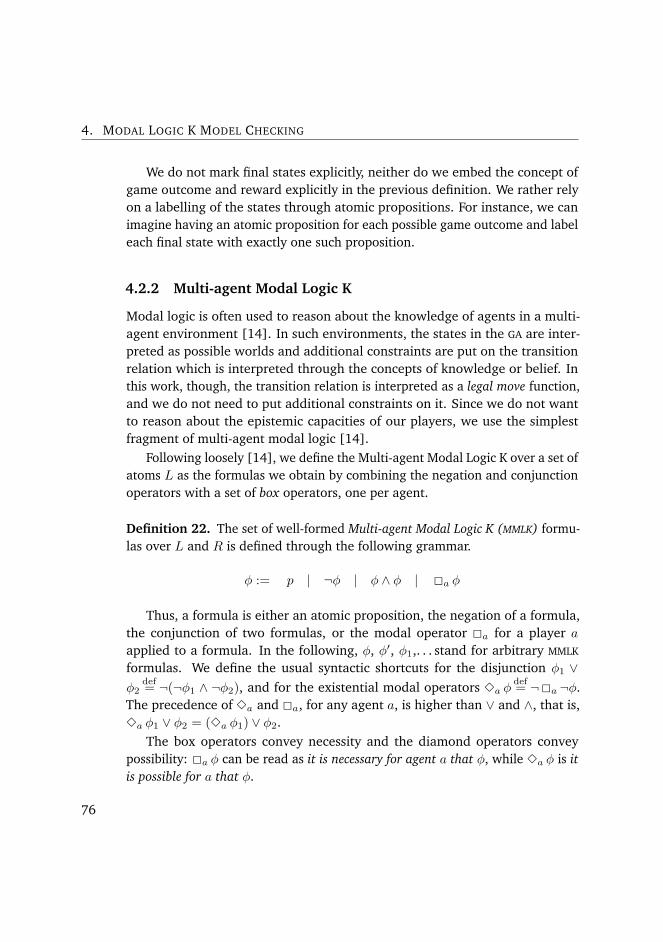
4. MODAL LOGIC K MODEL CHECKING
We do not mark final states explicitly, neither do we embed the concept of
game outcome and reward explicitly in the previous definition. We rather rely
on a labelling of the states through atomic propositions. For instance, we can
imagine having an atomic proposition for each possible game outcome and label
each final state with exactly one such proposition.
4.2.2 Multi-agent Modal Logic K
Modal logic is often used to reason about the knowledge of agents in a multi-
agent environment [14]. In such environments, the states in the GA are inter-
preted as possible worlds and additional constraints are put on the transition
relation which is interpreted through the concepts of knowledge or belief. In
this work, though, the transition relation is interpreted as a legal move function,
and we do not need to put additional constraints on it. Since we do not want
to reason about the epistemic capacities of our players, we use the simplest
fragment of multi-agent modal logic [14].
Following loosely [14], we define the Multi-agent Modal Logic K over a set of
atoms L as the formulas we obtain by combining the negation and conjunction
operators with a set of box operators, one per agent.
Definition 22. The set of well-formed Multi-agent Modal Logic K (MMLK) formu-
las over L and R is defined through the following grammar.
φ := p | ¬φ | φ ∧ φ | 2a φ
Thus, a formula is either an atomic proposition, the negation of a formula,
the conjunction of two formulas, or the modal operator 2a for a player a
applied to a formula. In the following, φ, φ′, φ1,. . . stand for arbitrary MMLK
formulas. We define the usual syntactic shortcuts for the disjunction φ1 ∨φ2
def= ¬(¬φ1 ∧ ¬φ2), and for the existential modal operators 3a φ
def= ¬2a ¬φ.
The precedence of 3a and 2a, for any agent a, is higher than ∨ and ∧, that is,
3a φ1 ∨ φ2 = (3a φ1) ∨ φ2.
The box operators convey necessity and the diamond operators convey
possibility: 2a φ can be read as it is necessary for agent a that φ, while 3a φ is it
is possible for a that φ.
76

4.2. Definitions
4.2.3 The Model Checking Problem
We can now interpret MMLK formulas over GAs via the satisfaction relation |=.
Intuitively, a state in a GA constitutes the context of a formula, while a formula
constitutes a property of a state. A formula might be satisfied in some contexts
and not satisfied in other contexts, and some properties hold in a state while
others do not. Determining whether a given formula φ holds in a given state q
(in a given implicit GA) is what is commonly referred to as the model checking
problem. If it is the case, we write q |= φ, otherwise we write q 6|= φ.
It is possible to decide whether q |= φ by examining the structure of φ, the
labels of q, as well as the accessible states.
Definition 23. The formulas satisfied by a state q can be constructed by induc-
tion as follows.
• If p is a label of q, that is if p ∈ λ(q), then q |= p;
• if q 6|= φ then q |= ¬φ;
• if q |= φ1 and q |= φ2 then q |= φ1 ∧ φ2;
• if for all q′ such that qa−→ q′, we have q′ |= φ, then q |= 2a φ.
It can be shown that the semantics for the syntactic shortcuts defined previ-
ously behave as expected. q |= φ1∨φ2 if and only if q |= φ1 or q |= φ2; q |= 3a φ
if there exists a q′ such that qa−→ q′ and q′ |= φ.
This semantical interpretation of MMLK allow an alternative understanding
of the box and diamond operators. We can also read 2a φ as all moves for agent
a lead to states where φ holds and read 3a φ as there exists a move for agent a
leading to a state where φ holds.
4.2.4 Proofs and Counterexamples
In practice, we never explicitly construct the complete set of formulas satisfied
by a state. So when some computation tells us that a formula φ is indeed (not)
satisfied by a state q, some sort of evidence might be desirable. In software
model checking, a model of the program replaces the GA, and a formula in a
temporal logic acts as a specification of the program. If a correct model checker
asserts that the program does not satisfy the specification, it means that the
77

4. MODAL LOGIC K MODEL CHECKING
program or the specification contained a bug. In those cases, it can be very
useful for the programmers to have access to an evidence by the model checker
of the mismatch between the formula and the system as it is likely to lead them
to the bug.
In this section we give a formal definition of what constitutes a proof or
a disproof for the class of model checking problems we are interested in. It
is possible to relate the following definitions to the more general concept of
tree-like counterexamples used in model checking ACTL [33].
Definition 24. An exploration tree for a formula φ in a state q is a tree with
root n associated with a pair (q, φ) with q a state and φ a formula, such that n
satisfies the following properties.
• If n is associated with (q, p) with p ∈ L, then it has no children;
• if n is associated with (q,¬φ) then n has at most one child and it is an
exploration tree associated with (q, φ);
• if a node n is associated with (q, φ1 ∧ φ2) then any child of n (if any) is an
exploration tree associated with (q, φ1) or with (q, φ2);
• if a node n is associated with (q,2a φ) then any child of n (if any) is an
exploration tree associated with (q′, φ) for some q′ such that qa−→ q′.
• In any case, no two children of n are associated with the same pair.
Unless stated otherwise, we will not distinguish between a tree and its root
node. In the rest of the paper, n, n′, n1, . . . will be used to denote nodes in
exploration trees.
Definition 25. A proof (resp. a disproof) that q |= φ is an exploration tree with
a root n associated with (q, φ) satisfying the following hypotheses.
• If φ = p with p ∈ L, then p ∈ λ(q) (resp. p /∈ λ(q));
• if φ = ¬φ′, then n has exactly one child n′ and this child is a disproof
(resp. proof);
• if φ = φ1 ∧ φ2, then n has exactly two children n1 and n2 such that n1 is a
proof that q |= φ1 and n2 is a proof that q |= φ2 (resp. n has exactly one
child n′ and n′ is a disproof that q |= φ1 or n′ is a disproof that q |= φ2);
78

4.2. Definitions
• if φ = 2a φ′, then n has exactly one child n′ for each q
a−→ q′, and n′ is a
proof for q′ |= φ′ (resp. n has exactly one child n′ and n′ is a disproof for
q′ |= φ′ for some qa−→ q′).
4.2.5 Cost Functions
To remain as general as possible with respect to the definitions of a small
(dis)proof in the introduction, we introduce a cost function k as well as cost
aggregators A∧ and A2. These functions can then be instantiated in a domain
dependent manner to get the optimal algorithm for the domain definition of
minimality. This approach has been used before in the context of A* and
AO* [111].
We assume given a base cost function k : L→ R+, as well as a conjunction
cost aggregator A∧ : NR+∪{∞} → R
+ ∪ {∞} and a box modal cost aggregator
A2 : Σ× NR
+∪{∞} → R+ ∪ {∞}, where N
R+∪{∞} denotes the set of multisets
of R+ ∪ {∞}.We assume the aggregators are increasing in the sense that adding elements
to the input increases the cost. For all costs x ≤ y ∈ R+ ∪ {∞}, multisets of
costs X ∈ NR
+∪{∞}, and for all agents a, we have for the conjunction cost
aggregator A∧(X) ≤ A∧({x} ∪X) ≤ A∧({y} ∪X), and for the box aggregator
A2(a,X) ≤ A2(a, {x} ∪X) ≤ A2(a, {y} ∪X).
We further assume that aggregating infinite costs results in infinite costs
and that aggregating finite numbers of finite costs results in finite costs. For all
costs x ∈ R+, multisets of costs X ∈ N
R+∪{∞}, and for all agents a, A∧({∞}) =
A2(a, {∞}) =∞ and that A∧(X) <∞⇒ A∧({x} ∪X) <∞ and A2(a,X) <
∞⇒ A2(a, {x} ∪X) <∞.
Note that in our presentation, there is no cost to a negation. The justification
is that we want a proof aggregating over a disjunction to cost as much as a
disproof aggregating over a conjunction with children of the same cost, without
having to include the disjunction and the diamond operator in the base syntax.
Given k, A∧, and A2, it is possible to define the global cost function for a
(dis)proof as shown in Table 4.1.
Example 8. Suppose we are interested in the nested depth of the 2 operators
in the (dis)proof. Then we define k = 0, A∧ = max, and A2(a,X) = 1+maxX
for all a.
79

4. MODAL LOGIC K MODEL CHECKING
Table 4.1: Cost K of a proof or a disproof for a node n as a function of the basecost function k and the aggregators A∧ and A2. C is the set of children of n.
Label of n Children of n K(n)
(q, p) ∅ k(p)(q,¬φ) {c} K(c)(q, φ1 ∧ φ2) C A∧({K(c)|c ∈ C})(q,2a φ) C A2(a, {K(c)|c ∈ C})
Example 9. Suppose we are interested in the number of atomic queries to
the underlying system (the GA). Then we define k = 1, A∧(X) =∑X, and
A2(a,X) =∑X for all a.
Example 10. Suppose we are interested in minimizing the amount of expansive
interactions with the underlying system. Then we define A∧(X) =∑X, and
A2(a,X) = k2a+∑X for all a. In this case, we understand that k(p) is the
price for querying p in any state, and k2ais the price for getting access to the
transition function for agent a in any state.
4.3 Model Checking Algorithms
We now define several model checking algorithms. That is, we present algo-
rithms that allow to decide whether a state q satisfies a formula φ (q |= φ).
4.3.1 Depth First Proof Search
Checking whether a formula is satisfied on a state can be decided by a depth-first
search on the game tree as dictated by the semantics given in Section 4.2.2.
Pseudo-code for the resulting algorithm, called Depth First Proof Search (DFPS)
is presented in Algorithm 7.
4.3.2 Best-first Search Algorithms
We can propose several alternatives to the DFPS algorithm to check a given
formula in a given state. We adapt the generic Best First Search (BFS) framework
proposed in Chapter 2 to express model checking algorithms. Best-first search
80

4.3. Model Checking Algorithms
Algorithm 7: Pseudo-code for the DFPS algorithm.
dfps(state q, formula φ)switch on the shape of φ do
case p ∈ L return p ∈ λ(q)case φ1 ∧ φ2 return dfps(q, φ1) ∧ dfps(q, φ2)case ¬φ1 return ¬ dfps(q, φ1)case 2a φ1
foreach q′ in {q′, q a−→ q′} doif not dfps(q′, φ1) then return false
return true
algorithms must maintain a partial tree in memory, the shape of which is
determined by the formula to be checked.
Nodes are mapped to a (state q, formula φ) label. A leaf is terminal if its
label is an atomic proposition p ∈ λ otherwise it is non-terminal. Each node is
associated to a unique position, but a position may be associated to multiple
nodes. 2
The following static observations can be made about partial trees:
• an internal node labelled (q,¬φ) has exactly one child and it is labelled
(q, φ);
• an internal node labelled (q, φ1 ∧ φ2) has exactly two children which are
labelled (q, φ1) and (q, φ2);
• an internal node labelled (q,2a φ) has as many children as there are
legal transition for a in q. Each child is labelled (q′, φ) where q′ is the
corresponding state.
The generic framework is described in Algorithm 8. An instance must
provide a data type for node specific information which we call node value and
the following procedures. The info-term defines the value of terminal leaves.
The init-leaf procedure is called when initialising a new leaf. The update
2While it is possible to store the state q associated to a node n in memory, it usually is moreefficient to store move information on edges and reconstruct q from the root position and the pathto n.
81

4. MODAL LOGIC K MODEL CHECKING
Algorithm 8: Pseudo-code for a best-first search algorithm.
extend(node n)switch on the shape of n.formula do
case φ1 ∧ φ2foreach i in {1, 2} do
ni ← new nodeni.state← q ; ni.formula← φi ; ni.info← ζ(q, φi)Add ni as childi of n
case ¬φn′ ← new noden′.state← q ; n′.formula← φ ; n′.info← ζ(q, φ)Add n′ as the child of n
case 2a φ
foreach q′ in {q′, n.statea−→ q′} do
n′ ← new noden′.state← q′ ; n′.formula← φ ; n′.info← ζ(q′, φ)Add n′ to n.children
backpropagate(node n)old info← n.infoswitch on the shape of n.formula do
case φ1 ∧ φ2 n.info← H∧(n.child1, n.child2)case ¬φ n.info← H¬(n.child)case 2a φ n.info← H2(n.children)
if old info = n.info ∨ n = r then return nelse return backpropagate(n.parent)
bfs(state q, formula φ)r ← new noder.state← q ; r.formula← φ ; r.info← ζ(q, φ)n← rwhile r.info /∈ S do
while n is not a leaf doswitch on the shape of n.formula do
case φ1 ∧ φ2 n← max4n.info∧
{n.child1, n.child2}case ¬φ n← n.childcase 2a φ n← max4n.info
2
{n.children}n← select-child(n)
extend(n)n← backpropagate(n)
return r82
4.3. Model Checking Algorithms
procedure determines how the value of an internal node evolves as a function
of its label and the value of the children. The select-child procedure decides
which child is best to be explored next depending on the node’s value and label
and the value of each child. We present possible instances in Sections 4.3.3 and
4.3.4.
The backpropagate procedure implements a small optimization known as
the current node enhancement [4]. Basically, if the information about a node n
are not changed, then the information about the ancestors of n will not change
either and so the next descend will reach n. Thus, it is possible to shortcut the
process and start the next descent at n directly.
4.3.3 Proof Number Proof Search
We present a first instance of the generic best-first search algorithm described
in Section 4.3.2 under the name Proof Number Proof Search (PNPS). This
algorithm uses the concept of effort numbers and is inspired from Proof Number
Search (PNS) [4, 155].
The node specific information needed for PNPS is a pair of numbers which
can be positive, equal to zero, or infinite. We call them proof number (p) and
disproof number (d). Basically, if a subformula φ is to be proved in a state s and
n is the corresponding node in the constructed partial tree, then the p (resp. d)
in a node n is a lower bound on the number of nodes to be added to the tree to
be able to exhibit a proof that s |= φ (resp. s 6|= φ). When the p reached 0 (and
the d reaches∞), the fact has been proved and when the p reached∞ (and the
d reaches 0) the fact has been disproved.
The info-term and init-leaf procedures are described in Table 4.2, while
Table 4.3 and 4.4 describe the update and select-child procedures, respec-
tively. If domain specific information is available, we can initialize the p and d
in init-leaf with heuristical values.
4.3.4 Monte Carlo Proof Search
MCTS is a recent game tree search technique based on multi-armed bandit
problems [20]. MCTS has enabled a huge leap forward in the playing level
of artificial GO players. It has been extended to prove wins and losses under
83

4. MODAL LOGIC K MODEL CHECKING
Table 4.2: Initial values for leaf nodes in PNPS.
Node label p d
info-term(q, p) when p ∈ λ(q) 0 ∞(q, p) when p /∈ λ(q) ∞ 0
init-leaf (q, φ) 1 1
Table 4.3: Determination of values for internal nodes in PNPS.
Node label Children p d
(q,¬φ) {c} d(c) p(c)(q, φ1 ∧ φ2) C
∑
C p minC d(q,2a φ) C
∑
C p minC d
Table 4.4: Selection policy for PNPS.
Node label Children Chosen child
(q,¬φ) {c} c(q, φ1 ∧ φ2) C argminC d(q,2a φ) C argminC d
the name MCTS Solver [165] and it can be seen as the origin of the algorithm
presented in this section which we call Monte Carlo Proof Search (MCPS).
The basic idea in MCPS is to evaluate whether a state s satisfies a formula via
probes in the tree below s. Monte Carlo probes are a generalization of Monte
Carlo playouts used in MCTS. A Monte Carlo playout is a random path of the
tree below s, whereas a Monte Carlo probe is a random subtree with a shape
determined by an MMLK formula. A probe is said to be successful if the formulas
at the leaves are satisfied in the corresponding states. Determining whether a
new probe generated on the fly is successful can be done as demonstrated in
Algorithm 9.
Like MCTS, MCPS explores the GA in a best first way by using aggregates of
information given by the playouts. For each node n, we need to know the total
number of probes rooted below n (denoted by t) and the number of successful
probes among them (denoted by r). We are then faced with an exploration-
84

4.4. Minimal Proof Search
Algorithm 9: Pseudo-code for a Monte Carlo Probe.
probe(state q, formula φ)switch on the shape of φ do
case p ∈ Lreturn p ∈ λ(q)
case φ1 ∧ φ2return probe(q, φ1) ∧ probe(q, φ2)
case ¬φ1return ¬ probe(q, φ1)
case 2a φ1q′ ← random state such that q
a−→ q′
return probe(q′, φ1)
Table 4.5: Initialisation for leaf values in MCPS for a node n.
Node label s r t
info-term(q, p) where p ∈ λ(q) ⊤ 1 1(q, p) where p /∈ λ(n) ⊥ 0 1
init-leaf (q, φ) ? probe(q, φ) 1
exploitation dilemma between running probes in nodes which have not been
explored much (t is small) and running probes in nodes which seem successful
(high rt
ratio). This concern is addressed using the UCB formula [20].
Similarly to MCTS Solver, we will add another label to the value of nodes
called s. s represents the proof status and allows to avoid solved subtrees.
s can take three values: ⊤, ⊥, or ?. These values respectively mean that
the corresponding subformula was proved, disproved, or neither proved nor
disproved for this node.
We describe the info-term, init-leaf, update, and select-child proce-
dures in Table 4.5, Table 4.6, and Table 4.7.
4.4 Minimal Proof Search
Let q |= φ be a model checking problem and n1 and n2 two proofs as defined in
Section 4.2.4. Even if n1 is not a subtree of n2, there might be reasons to prefer,
85

4. MODAL LOGIC K MODEL CHECKING
Table 4.6: Determination of values for internal nodes in MCPS.
Node label Children s r t
(q,¬φ) {c} ¬s(c) t(c)− r(c) t(c)(q, φ1 ∧ φ2) C
∧
C s∑
C r∑
C t(q,2a φ) C
∧
C s∑
C r∑
C t
Table 4.7: Selection policy for MCPS in a node n.
Node label Children Chosen child
(q,¬φ) {c} c
(q, φ1 ∧ φ2) C argmaxC,s(c)=?t−rt
+√
2 ln t(n)t
(q,2a φ) C argmaxC,s(c)=?t−rt
+√
2 ln t(n)t
n1 over n2. For instance, we can imagine that n1 contains fewer nodes than n2,
or that the depth of n1 is smaller than that of n2.
In this chapter, we put forward a model checking algorithm for MMLK that
we call Minimal Proof Search (MPS). As the name indicates, given a model
checking problem q |= φ, the MPS algorithm outputs a proof that q satisfies φ or
a counterexample, this proof/counterexample being minimal for some definition
of size. Perfect information games provide at least two motivations for small
proofs. In game playing, people are usually interested in “short” proofs, for
instance a CHESS player would rather deliver checkmate in three moves than
in nine moves even if both options grant them the victory. In game solving,
“compact” proofs can be stored and independently checked efficiently.
Our goal is related both to heuristic search and software model checking.
On one hand, the celebrated A* algorithm outputs a path of minimal cost from
a starting state to a goal state. This path can be seen as the proof that the
goal state is reachable, and the cost of the path is the size of the proof. On the
other hand, finding small counterexamples is an important subject in software
model checking. For a failure to meet a specification often indicates a bug in
the program, and a small counterexample makes finding and correcting the bug
easier [59].
Like A*, MPS is optimal, in the sense that any algorithm provided with the
86

4.4. Minimal Proof Search
Table 4.8: Definition of the heuristic functions I and J .
Shape of φ I(φ) J(φ)
p k(p) k(p)¬φ′ J(φ′) I(φ′)φ1 ∧ φ2 A∧({I(φ1), I(φ2)}) mini∈{1,2}A∧({J(φi)})2a φ
′ A2(a, ∅) A2(a, {J(φ′)})
same information and guaranteed to find a proof of minimal size needs to do as
many node expansions as MPS.
4.4.1 Heuristics
We define two heuristic functions I and J to estimate the minimal amount of
interaction needed with the underlying system to say anything about a formula
φ. These functions are defined in Table 4.8, I(φ) is a lower bound on the
minimal amount of interaction to prove φ and J(φ) is a lower bound on the
minimal amount of interaction to disprove φ.
The heuristics I and J are admissible, that is, they never overestimate the
cost of a (dis)proof.
Proposition 23. Given a formula φ, for any state q, for any proof n that q |= φ
(resp. disproof), I(φ) ≤ K(n) (resp. J(φ) ≤ K(n)).
Proof. We proceed by structural induction on the shape of formulas. For the
base case φ = p, if n is a proof that q |= p, then the n label of n is (q, p) and its
cost is K(n) = k(p), which is indeed greater or equal to I(p) = J(p) = k(p).
For the induction case, take the formulas φ1 and φ2 and assume that for any
proofs (resp. disproofs) n1 and n2, the cost is greater than the heuristic value:
I(φ1) ≤ K(n1) and I(φ2) ≤ K(n2) (resp. J(φ1) ≤ K(n1) and J(φ2) ≤ K(n2)).
For any proof (resp. disproof) nwith label (q,¬φa) and child c, the cost of n is
the cost of the disproof (resp. proof) c: K(n) = K(c). The disproof (resp. proof)
c is associated with (q, φ1) and we know from the induction hypothesis that
J(φ1) ≤ K(c) (resp. I(φ1) ≤ K(c)). By definition of the heuristics, I(φ) = J(φ1)
(resp. J(φ) = I(φ1)), therefore we have I(φ) ≤ K(n) (resp. J(φ) ≤ K(n)).
87
4. MODAL LOGIC K MODEL CHECKING
For any proof (resp. disproof) n with label (q, φ1 ∧ φ2) and children c1, c2(resp. child c), the cost of n is the sum of the costs of the children: K(n) =
K(c1) + K(c2) (resp. K(n) = K(c)). The nodes c1 and c2 are associated
with (q, φ1) and (q, φ2) (resp. c is associated with (q, φ1) or to (q, φ2)) and we
know from the induction hypothesis that I(φ1) ≤ K(c1) and I(φ2) ≤ K(c2)
(resp. J(φ1) ≤ K(c) or J(φ2) ≤ K(c)). By definition of the heuristics, I(φ) =
I(φ1)+I(φ2) (resp. J(φ) = min{J(φ1), J(φ2)}), therefore we have I(φ) ≤ K(n)
(resp. J(φ) ≤ K(n)).
The remaining case is very similar and is omitted.
Lemma 1. For any formula φ, I(φ) <∞ and J(φ) <∞.
Proof. We proceed by structural induction on φ. For the base case, φ = p, simply
recall that the range of k is R+. The induction case results directly from the
assumptions on the aggregators.
We inscribe the MPS algorithm in a best first search framework inspired
by game tree search. We then specify a function for initializing the leaves, a
function to update tree after a leaf has been expanded, a selection function to
decide which part of the tree to expand next, and a stopping condition for the
overall algorithm.
Algorithm 8 develops an exploration tree for a given state q and formula
φ. To be able to orient the search efficiently towards proving or disproving the
model checking problem q |= φ instead of just exploring, we need to attach
additional information to the nodes beyond their (state, formula) label. This
information takes the form of two effort numbers, called the minimal proof
number and minimal disproof number. Given a node n associated with a pair
(q, φ), the minimal proof number of n, MPN(n), is an indication on the cost of a
proof for q |= φ. Conversely, the minimal disproof number of n, MDN(n), is an
indication on the cost of a disproof for q |= φ. For a more precise relationship
between MPN(n) and the cost of a proof see Prop. 28.
The algorithm stops when the minimal (dis)proof number reaches∞ as it
corresponds to the exploration tree containing a (dis)proof of minimal cost (see
Prop. 26).
The values for the effort numbers in terminal leaves and in newly created
leaves are defined in Table 4.9. The values for the effort numbers of an internal
88

4.4. Minimal Proof Search
Table 4.9: Values for terminal nodes and initial values for leaves.
Node label MPN MDN
info-term(q, p) where p ∈ λ(q) k(p) ∞(q, p) where p /∈ λ(q) ∞ k(p)
init-leaf (q, φ) I(φ) J(φ)
Table 4.10: Determination of values for internal nodes.
Node label Children MPN MDN
(q,¬φ) {c} MDN(c) MPN(c)(q, φ1 ∧ φ2) C A∧({MPN(c)|c ∈ C}) minC A∧({MDN})(q,2a φ) C A2(a, {MPN(c)|c ∈ C}) minC A2(a, {MDN})
Table 4.11: Selection policy.
Node label Children Chosen child
(q,¬φ) {c} c(q, φ1 ∧ φ2) C argminC A∧({MDN})(q,2a φ) C argminC A2(a, {MDN})
node as a function of its children are defined in Table 4.10. Finally, the selection
procedure base on the effort numbers to decide how to descend the global tree
is given in Table 4.11. The stopping condition, Table 4.9, 4.10, and 4.11, as
well as Algorithm 8 together define Minimal Proof Search (MPS).
Before studying some theoretical properties of (dis)proofs, minimal (dis)proof
numbers, and MPS, let us point out that for any exploration tree, not necessarily
produced by MPS, we can associate to each node an MPN and an MDN by
using the initialization described in Table 4.9 and the heredity rule described in
Table 4.10.
4.4.2 Correctness
The first property we want to prove about MPS is that the descent does not get
stuck in a solved subtree.
89

4. MODAL LOGIC K MODEL CHECKING
Proposition 24. For any internal node n with finite effort numbers, the child
c selected by the procedure described in Table 4.11 has finite effort numbers.
MPN(n) 6=∞ and MDN(n) 6=∞ imply MPN(c) 6=∞ and MDN(c) 6=∞.
Proof. If the formula associated with n has shape ¬φ, then MDN(c) = MPN(n) 6=∞ and MPN(c) = MDN(n) 6=∞.
If the formula associated with n is a conjunction, then it suffices to note that
no child of n has an infinite minimal proof number and at least one child has a
finite minimal disproof number, and the result follows from the definition of the
selection procedure. This also holds if the formula associated with n is of the
form 2a φ′.
As a result, each descent ends in a non solved leaf. Either the associated
formula is of the form p and the leaf gets solved, or the leaf becomes an internal
node and its children are associated with structurally smaller formulas.
Proposition 25. The MPS algorithm terminates in a finite number of steps.
Proof. Let F be the set of lists of formulas ordered by decreasing structural
complexity, that is, F = {l = (φ0, . . . , φn)|n ∈ N, φ0 ≥ · · · ≥ φn}. Note that the
lexicographical ordering (based on structural complexity) <F is wellfounded
on F . Recall that there is no infinite descending chains with respect to a
well-founded relation.
Consider at some time t the list lt of formulas associated with the non
solved leaves of the tree. Assuming that lt is ordered by decreasing structural
complexity, we have lt ∈ F . Observe that a step of the algorithm results in a list
lt+1 smaller than lt according to the lexicographical ordering and that successive
steps of the algorithm result in a descending chain in F . Conclude that the
algorithm terminates after a finite number of steps for any input formula φ with
associated list l0 = (φ).
Since the algorithm terminates, we know that the root of the tree will
eventually be labelled with a infinite minimal (dis)proof number and thus will
be solved. It remains to be shown that this definition of a solved tree coincides
with containing (dis)proof starting at the root.
90

4.4. Minimal Proof Search
Proposition 26. If a node n is associated with (q, φ), then MDN(n) =∞ (resp.
MPN(n) = ∞) if and only if the tree corresponding to n contains a proof (resp.
disproof) that q |= φ as a subtree with root n.
Proof. We proceed by structural induction on the shape of trees.
For the base case when n has no children, either φ = p or φ is not atomic.
In the first case, n is a terminal node so contains a (dis)proof (n itself) and we
obtain the result by definition of MPN nad MDN as per Table 4.9. In the second
case, φ is not atomic and n has no children so n does not contain a proof nor a
disproof. Table 4.9 and Lemma 1 show that the effort numbers are both finite.
For the induction case when φ = ¬φ′, we know that n has one child c
associated to φ′. If c contains a proof (resp. disproof) that q |= φ′, then n
contains a disproof (resp. proof) that q |= φ. By induction hypothesis, we know
that MPN(c) =∞ (resp. MDN(c) =∞) therefore, using Table 4.10, we know
that MDN(n) = ∞ (resp. MPN(n) = ∞). Conversely if c does not contain a
proof nor a disproof, then n does not contain a proof nor a disproof, and we know
from the induction hypothesis and Table 4.10 than MPN(n) = MDN(c) < ∞and MDN(n) = MPN(c) <∞.
The other induction cases are similar but make use of the assumption that
aggregating inifinite costs results in infinite costs and that aggregating finite
numbers of finite costs results in finite costs.
Theorem 5. The MPS algorithm takes a formula φ and a state q as arguments and
returns after a finite number of steps an exploration tree that contains a (dis)proof
that q |= φ.
4.4.3 Minimality of the (Dis)Proofs
Now that we know that MPS terminates and returns a tree containing a (dis)proof,
we need to prove that this (dis)proof is of minimal cost.
The two following propositions can be proved by a simple structural induc-
tion on the exploration tree, using Table 4.9 and the admissibility of I and J for
the base case and Table 4.10 for the inductive case.
Proposition 27. If a node n is solved, then the cost of the contained (dis)proof is
given by the minimal (dis)proof number of n.
91

4. MODAL LOGIC K MODEL CHECKING
Proof. Straightforward structural induction on the shape of the tree using the
first half of Table 4.9 for the base case and Table 4.10 for the induction step.
Proposition 28. If a node n is associated with (q, φ), then for any proof m (resp.
disproof) that q |= φ, we have MPN(n) ≤ K(m) (resp. MDN(n) ≤ K(m)).
Proof. Structural induction on the shape of the tree, using the second half of
Table 4.9 and the admissibility of I and J (Prop. 23) for the base case and
Table 4.10 for the inductive case.
Since the aggregators for the cost function are increasing functions, then
MPN(n) and MDN(n) are non decreasing as we add more nodes to the tree n.
Proposition 29. For each disproved internal node n in a tree returned by the MPS
algorithm, at least one of the children of n minimizing the MDN is disproved.
Sketch. If we only increase the minimal (dis)proof number of a leaf, then for
each ancestor, at least one of either the minimal proof number of the minimal
disproof number remains constant.
Take a disproved internal node n, and assume we used the selection pro-
cedure described in Table 4.11. On the iteration that lead to n being solved,
the child c of n selected was minimizing the MDN and this number remained
constant since MPN(c) raised from a finite value to∞.
Since the MDN of the siblings of c have not changed, then c is still minimiz-
ing the MDN after it is solved.
Theorem 6. The tree returned by the MPS algorithm contains a (dis)proof of
minimal cost.
4.4.4 Optimality
The MPS algorithm is not optimal in the most general sense because it is pos-
sible to have better algorithm in some cases by using transpositions, domain
knowledge, or logical reasoning on the formula to be satisfied.
For instance, take φ1 = 3a(p∧¬p) and φ2 some non trivial formula satisfied
in a state q. If we run the MPS algorithm to prove that q |= φ1∨φ2, it will explore
at least a little the possibility of proving q |= φ1 before finding the minimal proof
through φ2. We can imagine that a more “clever” algorithm would recognize
92
4.4. Minimal Proof Search
that φ1 is never satisfiable and would directly find the minimal proof through
φ2.
Another possibility to outperform MPS is to make use of transpositions to
shortcut some computations. MPS indeed explores structures according to the
MMLK formula shape, and it is well-known in modal logic that bisimilar structures
cannot be distinguished by MMLK formulas. It is possible to express an algorithm
similar to MPS that would take transpositions into account, adapting ideas from
PNS [139, 100, 73]. We chose not to do so in this article for simplicity reasons.
Still, MPS can be considered optimal among the programs that do not use
reasoning on the formula itself, transpositions or domain knowledge. Stating
and proving this property formally is not conceptually hard, but we have not
been able to find simple definitions and a short proof that would not submerge
the reader with technicalities. Therefore we decided only to describe the main
ideas of the argument from a high-level perspective.
Definition 26. A pair (q′, φ′) is similar to a pair (q, φ) with respect to an ex-
ploration tree n associated with (q, φ) if q′ can substitute for q and φ′ for φ in
n.
Let n associated with (q, φ) be an exploration tree with a finite MPN (resp.
MDN), then we can construct a pair (q′, φ′) similar to (q, φ) with respect to n
such that there is a proof that q′ |= φ′ of cost exactly MPN(n) (resp. a disproof
of cost MDN(n)).
Definition 27. An algorithm A is purely exploratory if the following holds. Call
n the tree returned by A when run on a pair (q, φ). For every pair (q′, φ′) similar
to (q, φ) with respect to n, running A on (q′, φ′) returns a tree structurally
equivalent to n.
Depth first search, if we were to return the explored tree, and MPS are both
examples of purely exploratory algorithms.
Proposition 30. If a purely exploratory algorithm A is run on a problem (q, φ)
and returns a solved exploration tree n where MPN(n) (resp. MDN(n)) is smaller
than the cost of the contained proof (resp. disproof), then we can construct a
problem (q′, φ′) similar with respect to n such that A will return a structurally
equivalent tree with the same proof (resp. disproof) while there exists a proof of
cost MPN(n) (resp. disproof of cost MDN(n)).
93

4. MODAL LOGIC K MODEL CHECKING
Note that if the cost of a solved exploration tree n is equal to its MPN (resp.
MDN), then we can make MPS construct a solved shared root subtree of n just
by influencing the tie-breaking in the selection policy described in Table 4.11.
Theorem 7. If a purely exploratory algorithm A returns a solved exploration tree
n, either this tree (or a subtree) can be generated by MPS or A is not guaranteed to
return a tree containing a (dis)proof of minimal cost on all possible inputs.
4.5 Sequential solution concepts in MMLK
We now proceed to define several classes of formulas to express interesting
properties about games.
We will assume for the remainder of the paper that one distinguished player
is denoted by A and the other players (if any) are denoted by B (or B1, . . . ,
Bk). Assume a distinguished atomic propositions w, understood as a label of
final positions won by A. We also use a variant of the normal play assumption,
namely, when a position s is won by A, no other player has a legal move in s.
When a position s is lost by A, then A has no legal moves in s but other players
have a pass move that loop to s. That is, for every state s lost by A, we have
sB−→ s.
Reachability A natural question that arises in one-player games is reachability.
In this setting, we are not interested in reaching a specific state, but rather in
reaching any state satisfying a given property.
Definition 28. We say that a player A can reach a state satisfying φ from a state
q in exactly n steps if q |= 3A . . .3A︸ ︷︷ ︸
n times
φ.
Winning strategy The concept of winning strategies in a finite number of
moves in an alternating two-player game can also be represented as as a
formula.
Definition 29. Player A has a winning strategy of depth less or equal to 2n+ 1
in state q if q |= ωn+1, where ω1 = w ∨3A w and ωn = w ∨3A2B ωn−1.
94

4.5. Sequential solution concepts in MMLK
(a) HEX position featuring a ladder for Black. (b) CHESS position featuring a helpmatefor Black in four moves.
Figure 4.1: Positions illustrating the solution concepts of ladder and helpmate.
Ladders The concept of ladder occurs in several games, particularly HEX and
GO [102]. A threatening move for player A is a move such that, if it was possible
for A to play a second time in a row, then A could win. A ladder is a sequence
of threatening moves by A followed by defending moves by B, ending with A
fulfilling their objective.
Definition 30. Player A has a ladder of depth less or equal to 2n+1 in state s if
q |= L2n+1, where L1 = w∨3A w and L2n+1 = w∨3A((w∨3A w)∧2B L2n−1).
For instance, Figure 4.1a presents a position of the game HEX where the goal
for each player is to connect their border by putting stones of their color. In this
position, Black can play a successful ladder thereby connecting the left group to
the bottom right border.
Helpmates In a CHESS helpmate, the situation seems vastly favourable to
player Black, but the problemist must find a way to have the Black king check-
mated. Both players move towards this end, so it can be seen as a cooperative
game. Black usually starts in helpmate studies. See Figure 4.1b for an example.
A helpmate in at most 2n plies can be represented through the formula Hn
where H0 = w and Hn = w ∨3B 3A Hn−1.
95

4. MODAL LOGIC K MODEL CHECKING
(a) HEX position featuring a progress tree of depth7 for Black.
(b) CHESS endgame featuring a progresstree of depth 11 for White.
Figure 4.2: Positions illustrating the concept of progress tree.
Selfmates A selfmate, on the other hand, is a situation where Black forces
White to checkmate the Black King, while White must do their best to avoid this.
Black starts moving in a selfmate and a position with a selfmate satifies Sn for
some n, where S0 = w and Sn = w ∨3B 2A Sn−1.
Progress Trees It occurs in many two-player games that at some point near
the end of the game, one player has a winning sequence of n moves that is
relatively independent of the opponent’s moves. For instance Figure 4.2 presents
a HEX position won for Black and a CHESS position won for White. In both cases,
the opponent’s moves cannot even delay the end of the game.
To capture this intuition, we define a new solution concept we name progress
tree. The idea giving its name to the concept of progress trees is that we want
the player to focus on those moves that brings them closer to a winning state,
and discard the moves that are out of the winning path.
Definition 31. Player A has a progress tree of depth 2n + 1 in a state q if
q |= PTn+1, where PT1 = w ∨3A w and PTn = w ∨3A(πn−1 ∧2B PTn−1).
We can check states for progress trees using any of the model checking
algorithms presented earlier, effectively giving rise to four new specialized
96

4.5. Sequential solution concepts in MMLK
Table 4.12: Search statistics for a DFPS on positions along a principal variationof the CHESS problem in Figure 4.2b.
Model checkingproblem
Time (s)Number of queries
atomic listmoves play
PT3 0.1 6040 328 5897ω3 0.2 11172 624 5587
PT4 1.4 99269 5312 98696ω4 3.5 194429 10621 97217
PT5 23.6 1674454 88047 1668752ω5 63.8 3382102 181442 1691055
PT6 260.4 25183612 1297975 25106324ω6 953.6 52209939 2759895 26104986
algorithms. Note that if a player has a progress tree of depth 2n + 1 in some
state, then they also have a winning strategy of depth 2n + 1 from that state
(see Proposition 31). Therefore, if we prove that a player has a progress tree in
some position, then we can deduce that they have a winning strategy.
We tested a naive implementation of the DFPS model checking algorithms on
the position in Figure 4.2b to check for progress trees and winning strategies.
The principal variations consists for White in moving the pawn up to the last
row and move the resulting queen to the bottom-right hand corner to deliver
checkmate. To study how the solving difficulty increases with respect to the size
of the formula to be checked, we model checked every position on a principal
variation and present the results in Table 4.12.
We can see that proving that a progress tree exists becomes significantly
faster than proving an arbitrary winning strategy as the size of the problem
increases. We can also notice that the overhead of checking for a path at each α
node of the search is more than compensated by the early pruning of moves not
contributing to the winning strategy.
97

4. MODAL LOGIC K MODEL CHECKING
4.6 Understanding game tree algorithms
We now turn to show how the MMLK Model Checking framework can be used
to develop new research in game tree search. As such, the goal of this section
is not to put forward a single well performing algorithm, nor to prove difficult
theorems with elaborate proofs, but rather to demonstrate that the MMLK Model
Checking is an appropriate tool for designing and reasoning about new game
tree search algorithms.
By defining appropriate formulas classes, we can simulate many existing
algorithms by solving model checking problems in MMLK with specific search
algorithms.
Definition 32. Let φ be a formula, S be a model checking algorithm and A be
a specific game algorithm. We say that (φ, S) simulates A if for every game, for
every state q where A can be applied, we have the following: solving q |= φ
with S will explore exactly the same states in the same order and return the
same result as algorithm A applied to initial state q.
Table 4.13 presents how combining the formulas defined later in this section
with model checking algorithms for MMLK allows to simulate many important
algorithms. We use the model checking algorithms defined in Section 4.3,
DFPS, PNPS, and MCPS as well as MPS proposed by Saffidine [119]. For instance,
using the DFPS algorithm to model-check an APSn formula on a HEX position
represented as a state of a GA is exactly the same as running the Abstract Proof
Search algorithm on that position.
4.6.1 One-player games
Many one-player games, the so-called puzzles, involve finding a path to a
terminal state. Ideally this path should be the shortest possible. Examples of
such puzzles include the 15-PUZZLE and RUBIK’S CUBE.
Recall that we defined a class of formulas for reachability in exactly n steps
in Definition 28. Similarly we define now a class of formulas representing the
existence of a path to a winning terminal state within n moves.
Definition 33. We say that agent A has a winning path from a state q if q
satisfies πn where πn is defined as π0 = w and πn = w ∨3A πn−1 if n > 0.
98

4.6. Understanding game tree algorithms
Table
4.1
3:
Dif
fere
nt
alg
ori
thm
sexpre
ssed
as
aco
mbin
ati
on
of
afo
rmu
lacl
ass
an
da
searc
hpara
dig
m.
Form
ula
Mod
el
Ch
eck
ing
Alg
ori
thm
DFP
SP
NP
SM
CP
SM
PS
πn
Depth
-firs
tse
arc
hG
reed
yB
FS
[11
1]
Sin
gle
-pla
yer
MC
TS
[13
2]
A*
[60
]ωn
αβ
[75
]P
NS
[4]
MC
TS
solv
er
[16
5]
DFP
N+
[10
3]
PA
nPara
noid
[14
9]
Para
noid
PN
S[1
29
]M
ult
i-pla
yer
MC
TS
[10
5]
λd,n
Lam
bd
ase
arc
h[1
53
]Lam
bd
aP
NS
[16
9]1
βn
Best
reply
searc
h[1
30
]M
CT
S-B
RS
[10
6]
APSn
Abst
ract
pro
of
searc
h[2
3]
1W
eact
uall
yn
eed
toch
an
ge
the
upd
ate
rule
for
thep
inin
tern
alφ1∧φ2
nod
es
inP
NP
Sfr
om∑
Cp
tomax
Cp.
99

4. MODAL LOGIC K MODEL CHECKING
4.6.2 Two-player games
We already defined the winning strategy formulas ωn in Definition 29. We will
now express a few other interesting formulas that can be satisfied in states in
two player games.
λ-Trees λ-trees have been introduced [153] as a generalisation of ladders as
seen in Section 4.5. We will refrain from describing the intuition behind λ-trees
here and will be satisfied with giving the formal corresponding property as they
only constitute an example of the applicability of our framework.
Definition 34. A state q has an λ-tree of order d and maximal depth n for
player A if q |= λd,n, where λ0,n = λd,0 = w, λd,1 = w ∨ 3A w, and λd,n =
w ∨3A(λd−1,n−1 ∧2B λd,n−2).
λ-trees are a generalisation of ladders as defined in Definition 30 since a
ladder is a λ-tree of order d = 1.
Abstract proof trees Abstract proof trees were introduced to address some
perceived practical limitations of αβ when facing a huge number of moves.
They have been used to solve capture problems for the game of GO. We limit
ourselves here to describing how we can specify in MMLK that a state is root to
an an abstract proof tree. Again, we refer the reader to the literature for the
intuition about abstract proof trees and their original definition [23].
Definition 35. A state q has an abstract proof tree of order n for player A
if q |= APSn, where APS0 = w, APS1 = w ∨ 3A w, and APSn = w ∨3A(APSn−1 ∧2B APSn−1).
Other concepts Many other interesting concepts can be similarly implemented
via a class of appropriate formulas. Notably minimax search with iterative
deepening, the Null-move assumption, and Dual Lambda-search [145] can be
related to model checking some MMLK formulas with DFPS.
4.6.3 Multiplayer games
Paranoid Algorithm The Paranoid Hypothesis was developed to allow for
αβ style safe pruning in multiplayer games [149]. It transforms the original
100

4.6. Understanding game tree algorithms
k + 1-player game into a two-player game A versus B. In the new game, the
player B takes the place of B1, . . . , Bk and B is trying to prevent player A
from reaching a won position. Assuming the original turn order is fixed and is
A,B1, . . . , Bk, A,B1, . . . , we can reproduce a similar idea in MMLK.
Definition 36. Player A has a paranoid win of depth (k + 1)n in a state q if
q |= PAn,0, where PAn,0 is defined as follows.
PA0,i = w
PAn,0 = w ∨3A PAn−1,1
PAn,i = 2Bi PAn−1,i+1 for 1 ≤ i < k
PAn,k = 2Bk PAn−1,0
(4.1)
Observe that in a k + 1-player game, if 0 ≤ j < k then PA(k+1)n+j,j can be
expressed as 2Bj 2Bj+1 . . .2Bk PA(k+1)n,0
Best Reply Search Best Reply Search (BRS) is a new search algorithm for
multiplayer games [130]. It consists of performing a minimax search where
only one opponent is allowed to play after A. For instance a principal variation
in a BRS search with k = 3 opponents could involve the following turn order A,
B2, A, B1, A, B1, A, B3, A, . . . instead of the regular A, B1, B2, B3, A, B1, B2,
B3, . . . .
The rationale behind BRS is that the number of moves studied for the player
in turn in any variation should only depend on the depth of the search and not
on the number of opponents. This leads to an artificial player selecting moves
exhibiting longer term planning. This performs well in games where skipping
a move does not influence the global position too much, such as CHINESE
CHECKERS.
Definition 37. Player A has a best-reply search win of depth 2n+ 1 in a state q
if q |= βn, where β1 = w ∨3A w and βn = w ∨3A
∧k
i=12Bi βn−1.
4.6.4 Expressing properties of the algorithms
We now demonstrate that using the MMLK model checking framework for game
tree search makes some formal reasoning straightforward. Again, the goal of
101

4. MODAL LOGIC K MODEL CHECKING
this section is not to demonstrate strong theorems with elaborate proofs but
rather show that the framework is convenient for expressing certain properties
and helps reasoning on them.
It is easy to prove by induction on the depth that lambda trees, abstract proof
trees, and progress trees all have winning strategies as logical consequence.
Proposition 31. For all order d and depth n, we have |= λd,2n+1 → ωn+1,
|= APSn → ωn, and |= PTn → ωn.
Proof. We prove the implication between λ-trees and winning strategy by in-
duction on the depth n. The proofs for abstract proof trees and progress trees
are similar and are omitted.
Base case n = 0. If the depth is n = 0 then we have λd,1 = w ∨3A w and
ω1 = w ∨3A w so the property holds.
Induction case, assuming |= λd,2n+1 → ωn+1, let us show that |= λd,2n+3 →ωn+2. If d = 0, then λd,2n+3 = w so the property holds. Else, d > 0 and we
have λd,2n+3 = w ∨3A(λd−1,2n+2 ∧ 2B λd,2n+1). By induction hypothesis we
obtain |= λd,2n+3 → w ∨ 3A(λd−1,2n+2 ∧ 2B ωn+1). By weakening we have
|= λd,2n+3 → w ∨3A2B ωn+1, that is |= λd,2n+3 → w ∨ ωn+2.
Therefore, whenever we succeed in proving that a position features, say, an
abstract proof tree, then we know it also has a winning strategy for the same
player: for any state q, q |= APSn implies q |= ωn.
On the other hand, in many games, it is possible to have a position featuring
a winning strategy but no lambda tree, abstract proof tree, or even progress
tree. Before studying the other direction further, we need to rule out games
featuring zugzwangs, that is, positions in which a player would rather pass and
let an opponent make the next move.
Definition 38. A φ-zugzwang for player A against players B1, . . . , Bk is a state
q such that q |= ¬φ∧(∨i2Bi φ). A game is zugzwang-free for a set of formulas Φ
and player A against players B1, . . . , Bk if for every state q, and every formula
φ ∈ Φ, q is not a φ-zugzwang for A against B1, . . . , Bk.
We denote the set games that are zugzwang-free for Φ as Z(Φ). A formula
ψ is valid in zugzwang-free games for Φ, if for any game G in Z(Φ) and any
state s, we have G, s |= ψ. In such case we write |=Z(Φ) ψ.
102

4.6. Understanding game tree algorithms
We can use this definition to show that in games zugzwang-free for winning
strategies, such as CONNECT-6 or HEX, an abstract proof tree and a progress tree
are equivalent to a winning strategy of the same depth.
Proposition 32. Consider a two-player game zugzwang-free for winning strategies.
For any depth n and any state q, q |= ωn implies q |= APSn and q |= ωn
implies q |= PTn. That is |=Z(Φ) ωn → APSn and |=Z(Φ) ωn → PTn where
Φ = {ωi, i ∈ N}.
Proof. We prove the result involving abstract proof trees and winning strategies
by induction on n. The other result can obtained with a similar proof. Assume a
zugzwang-free game for winning strategies. We want to prove that for any state
q in the game, if q |= ωn then we have q |= APSnSince ω0 = APS0 = w, the property holds for the base case, n = 0.
Assume that for all q, q |= ωn implies q |= APSn, and take q such that
q |= ωn+1. Since ωn+1 = w ∨ 3A2B ωn then either q |= w in which case
q |= APSn+1 or we can find q′ such that q′ |= 2B WS and qA−→ q′. In this case,
it remains to prove that q′ |= APSn and q′ |= 2B APSn.
To show that q′ |= 2B APSn, consider q′′ such that q′B−→ q′′. We know that
q′ |= 2B ωn so q′′ |= ωn and by induction hypothesis, we have q′′ |= APSn.
To show that q′ |= APSn, recall that the game is zugzwang-free for winning
strategies, and in particular, it is zugzwang-free for ωn. It means that there
is no state q such that q |= ¬ωn ∧ 2B ωn. By taking q to be q′, we have
q′ |= ωn ∨ ¬2B ωn. Since we know that q′ |= 2B ωn we derive that q′ |= ωn.
The induction hypothesis allows us to conclude.
The usual understanding of zugzwang is in two player games with φ a
winning strategy formula or a formula representing forcing some material gain
in CHESS. The more general definition we have given allows for multiplayer
games and other solution concepts besides winning strategies. For instance, it is
possible to show that best reply wins are more common than paranoid wins in
games which are zugzwang-free for paranoid wins.
Proposition 33. Consider a multiplayer game with k + 1 players, zugzwang-free
for paranoid wins. For any depth n and any state q, q |= PA(k+1)n,0 implies
q |= βn. That is |=Z(Φ) PA(k+1)n,0 → βn where Φ = {PAi,j , i ∈ N, j ∈ N}.
103

4. MODAL LOGIC K MODEL CHECKING
As a result, in such a game, if a search for a best reply win fails, we know
there is no need to carry a search for a paranoid win. Since looking for a best
reply win of depth 2n + 1 is usually much faster than looking for a paranoid
win of depth (k + 1)n, this formal result can be seen as a partial explanation of
the experimental success of Best Reply Search in CHINESE CHECKERS [130].
4.6.5 Examining new combinations
We have seen that we could obtain previously known algorithms by combining
model checking algorithms with solution concepts. On the one hand, some
solution concepts such winning path and winning strategy, were combined with
the four possible search paradigms in previous work. On the other hand, other
solution concepts such as abstract proof trees were only investigated within the
depth-first paradigm.
It is perfectly possible to model check a paranoid win using the MCPS algo-
rithm, for instance, leading to a new Minimal Paranoid Win Search algorithm.
Similarly model checking abstract proof trees with PNPS would lead to a new
Proof Number based Abstract Proof Search (PNAPS) algorithm. Preliminary
experiments in HEX without any specific domain knowledge added seem to
indicate that PNAPS does not seem to perform as well as Abstract Proof Search,
though.
Finally, most of the empty cells in Table 4.13 can be considered as new
algorithms waiting for an optimized implementation and a careful evaluation.
4.7 Related work and discussion
In CTL model checking, finding a minimal witness or a minimal counterexample
is NP-complete [31]. MMLK model checking, on the contrary, though PTIME-
complete [84], allows finding minimal witnesses/counterexamples relatively
efficiently as we shall see in this chapter.
The tableau-based model checking approach by Cleaveland for the µ-calculus
seems to be similar to ours [34], however it would need to be adapted to
handle (dis)proof cost. Also, in our understanding, the proof procedure check1
presented by Cleaveland can be seen as an unguided Depth First Search (DFS)
while our approach is guided towards regions of minimal cost.
104

4.7. Related work and discussion
The two algorithms most closely related to MPS are AO*, a generalization
of A* to And/Or trees, and DFPN+ [103], a variant of DFPN, itself a depth-first
variant of PNS [4].
DFPN+ is typically only used to find a winning strategy for either player in
two-player games. MPS, on the contrary, can be applied to solve other interesting
problems without a cumbersome And/Or graph prior conversion. Example of
such problems range from finding ladders in two-player games to finiding
paranoid wins in multi-player games. Another improvement over DFPN+ is
that we allow for a variety of (dis)proof size definitions. While DFPN+ is set to
minimize the total edge cost in the proof, we can imagine minimizing, say, the
number of leaves or the depth of the (dis)proof.
Besides the ease of modelling allowed by MMLK rather than And/Or graphs,
another advantage of MPS over AO* is that if the problem is not solvable, then
MPS finds a minimal disproof while AO* does not provide such a guarantee.
In his thesis, Nagai derived the DFPN algorithm from the equivalent best-first
algorithm PNS [103]. Similarly, we can obtain a depth-first version of MPS from
the best first search version presented here by adapting Nagai’s transformation.
Such a depth-first version should probably be favoured in practice, however we
decided to present the best first version in this article for two main reasons. We
believe the best-first search presentation is more accessible to the non-specialists.
The proofs seemed to be easier to work through in the chosen setting, and they
can later be extended to the depth-first setting.
Another trend of related work is connecting modal logic and game the-
ory [157, 167, 81]. In this area, the focus is on the concept of Nash equilibria,
extensive form games, and coalition formation. As a result, more powerful
logic than the restricted MMLK are used [6, 159, 58]. Studying how the model
checking algorithms presented in this chapter can be extended for these settings
is an interesting path for future work.
We have shown that the Multi-agent Modal Logic K was a convenient tool to
express various kind of threats in a game independent way. Victor Allis provided
one of the earliest study of the concept of threats in his Threat space search
algorithm used to solve GOMOKU [5].
Previous work by Schaeffer et al. was also concerned with providing a
unifying view of heuristic search and the optimization tricks that appeared in
both single-agent search and two-player game search [134].
105

4. MODAL LOGIC K MODEL CHECKING
The model used in this chapter differs from the one used in GGP called
Multi-Agent Environment (MAE) [138]. In an MAE, a transition correspond to
a joint-action. That is, each player decide a move simultaneously and the
combination of these moves determines the next state. In a GA, as used in this
chapter, the moves are always sequential. It is possible to simulate sequential
moves in an MAE by using pass moves for the non acting agents, however this
ties the turn player into the game representation. As a result, testing for solution
concepts where the player to move in a given position is variable is not possible
with an MAE. For instance, it is not possible to formally test for the existence of
a ladder in a GGP representation of the game of GO because we need to compute
the successors of a given position after a white move and alternatively after a
black move.
We envision a depth-first adaptation of MPS similar to Nagai’s transformation
of PNS into DFPN. Alternatively, we can draw inspiration from PN2 [4] and
replace the heuristic functions I and J by a nested call to MPS, leading to an
MPS2 algorithm trading time for memory. These two alternative algorithms
would directly inherit the correctness and minimality theorems for MPS. The
optimality theorem would also transpose in the depth-first case, but it would not
be completely satisfactory. Indeed, even though the explored tree will still be
admissibly minimal, several nodes inside the tree will have been forgotten and
re-expanded multiple times. This trade-off is reminiscent of the one between A*
and its depth-first variation IDA* [78].
Representing problems with unit edge costs is already possible within the
framework presented in Section 4.2.5. It is not hard to adapt MPS to the more
general case as we just need to replace the agent labels on the transitions with
(agent, cost) labels. This more general perspective was not developed in this
chapter because the notation would be heavier while it would not add much to
the intuition and the general understanding of the ideas behind MPS.
Effective handling of transpositions is another interesting topic for future
work. It is already nontrivial in PNS [73] and MCTS [125], but it is an even richer
subject in this model checking setting as we might want to prove different facts
about a given position in the same search. Finding minimal (dis)proofs is more
challenging when taking transpositions into account because of the double count
problem. While it is possible to obtain a correct algorithm returning minimal
(dis)proofs by using functions based on propagating sets of individual costs
106

4.8. Conclusion
instead of real values in Section 4.2.5, similarly to previous work in PNS [100],
such a solution would hardly be efficient in practice and would not necessarily
be optimal. The existing literature on PNS and transpositions can certainly
be helpful in addressing efficient handling of transpositions in MMLK model
checking [139, 100, 73].
4.8 Conclusion
We have seen the MMLK was an appropriate framework for formal definitions of
solution concepts for perfect information games. We have shown that research
on game tree search could be a source of inspiration when designing algorithms
to solve the model checking problem for MMLK. Also, combining modal formulas
and a model checking algorithms yields a variety of game tree search algorithms
that can be modeled in the same framework. This makes it easy to test known
algorithms as well to define new ones. Finally, non-trivial properties of game
search algorithms can be proved in the modal logic formalism with just a few
formula manipulations.
Table 4.13 reveals many interesting previously untested possible combina-
tions of formula classes and search algorithms. Implementing and optimizing
one specific new combination for a particular game could lead to insightful
practical results. For instance, it is quite possible that a Proof Number version
of Abstract Proof Search would be successful in the capture game of GO [23].
We have also presented Minimal Proof Search (MPS), a model checking
algorithm for MMLK. MPS has been proven correct, and it has been proved that
the (dis)proof returned by MPS was minimizing a generic cost function. The
only assumption about the cost function is that it is defined recursively using
increasing aggregators. Finally, we have shown that MPS was optimal among
the purely exploratory model checking algorithms for MMLK.
Nevertheless, the proposed approach has a few limitations. MPS is a best
first search algorithm and is memory intensive; the cost functions addressed in
the chapter cannot represent variable edge cost; and MPS cannot make use of
transpositions in its present form. Still, we think that these limitations can be
overcome in future work.
Beside evaluating and improving the practical performance of MPS, future
work can also study to which extent the ideas presented in this chapter can be
107

4. MODAL LOGIC K MODEL CHECKING
applied to model checking problems in more elaborate modal logics and remain
tractable.
108

5 Games with Simultaneous Moves
This chapter defines and focuses on stacked-matrix games, that is
two-player zero-sum games featuring simultaneous moves. Alpha-
beta pruning can be generalized to stacked-matrix games, however
computing the alpha and beta bounds is costly as it involves solving
Linear Programs (LPs). We develop a few heuristical optimizations
that allow to mitigate the time spent solving LPs, eventually leading to
an algorithm solving GOOFSPIEL faster than backward induction and
sequence form solving.
The stacked-matrix games formalism can also model the combat phase
of Real-Time Strategy (RTS) games. However the time constraints
associated to building an Artificial Intelligence (AI) for an RTS game are
so tight that practical settings cannot be solved exactly. On the other
hand, we show that approximate heuristical search is possible and leads
to much better performance than existing script-based approaches.
This Chapter includes results from the following papers.
[127] Abdallah Saffidine, Hilmar Finnsson, and Michael Buro. Alpha-
beta pruning for games with simultaneous moves. In Hoffmann and
Selman [66], pages 556–562
[30] David Churchill, Abdallah Saffidine, and Michael Buro. Fast
heuristic search for RTS game combat scenarios. In Mark Riedl and Gita
Sukthankar, editors, 8th AAAI Conference on Artificial Intelligence
and Interactive Digital Entertainment (AIIDE), pages 112–117, Palo
Alto, California, USA, October 2012. AAAI Press
109

5. GAMES WITH SIMULTANEOUS MOVES
Contents
5.1 Stacked-matrix games . . . . . . . . . . . . . . . . . . . . . 110
5.1.1 Formal model . . . . . . . . . . . . . . . . . . . . . 111
5.1.2 Related game classes . . . . . . . . . . . . . . . . . 112
5.1.3 Modelling RTS game combat . . . . . . . . . . . . . 114
5.2 Solution Concepts for Stacked-matrix Games . . . . . . . . . 115
5.2.1 Backward induction and Nash equilibria . . . . . . . 115
5.2.2 Game Theoretic Approximations . . . . . . . . . . . 116
5.3 Simultaneous Move Pruning . . . . . . . . . . . . . . . . . . 120
5.3.1 Alpha-Beta Search . . . . . . . . . . . . . . . . . . . 124
5.3.2 Propagating Bounds . . . . . . . . . . . . . . . . . . 124
5.3.3 Main Algorithm . . . . . . . . . . . . . . . . . . . . 126
5.3.4 Ordering Move Pairs . . . . . . . . . . . . . . . . . 128
5.4 Fast approximate search for combat games . . . . . . . . . . 128
5.4.1 Scripted behaviors . . . . . . . . . . . . . . . . . . 129
5.4.2 Alpha-Beta Search with Durative Moves . . . . . . . 130
5.4.3 Evaluation Functions . . . . . . . . . . . . . . . . . 131
5.4.4 Move Ordering . . . . . . . . . . . . . . . . . . . . 133
5.5 Experiments . . . . . . . . . . . . . . . . . . . . . . . . . . 133
5.5.1 Solving GOOFSPIEL . . . . . . . . . . . . . . . . . . 133
5.5.2 Real-time Strategy games . . . . . . . . . . . . . . . 136
5.6 Conclusion and Future Work . . . . . . . . . . . . . . . . . 139
5.1 Stacked-matrix games
While search-based planning approaches have had a long tradition in the con-
struction of strong AI systems for abstract games like CHESS and GO, only in
recent years have they been applied to modern video games, such as First-Person
Shooter (FPS) and RTS games [108, 29].
In this chapter, we study two-player zero-sum games featuring simultaneous
moves called stacked-matrix games. We first show how it relates to the more
general class of MAE and that combat situations in RTS games can be seen as
110

5.1. Stacked-matrix games
stacked-matrix games. We then provide with an algorithm to perform safe
pruning in a depth-first search in this class of games, thus generalizing alpha-
beta pruning. Using this algorithm, we are able to solve GOOFSPIEL instances
more efficiently. In RTS games, the time constraints are tight and the goal is to
find a good move rather than to determine the value of the game. We therefore
show how efficient approximate search can be performed on stacked-matrix
games, focussing on RTS combat settings.
Classical abstract games such as CHESS or GO are purely sequential zero-sum
two-player games. To model some other games such as CHINESE CHECKERS it is
necessary to drop the two-player assumption. In this chapter, we study the class
of games obtained by dropping the pure sequentiality assumption.
5.1.1 Formal model
Definition 39. A stacked-matrix game is a transition system 〈S,R,−→, L, λ〉 in
which the following restriction holds:
• The set of transition labels can be seen as the cartesian square of a set of
moves M , R =M ×M ;
• The state labels are bounded real numbers, L ⊆ [b, a], where a ∈ R and
b ∈ R.
Stacked-matrix games are two-player games with simultaneous moves. The
interpretation of the transition relation is that when in a state s, both players
choose a move, say m1 and m2 and the resulting state s′ is obtained as a
combination of s and the joint move (m1,m2): sm1,m2−−−−→ s′.
A state is final, if it has no outgoing transitions. The set of final states is
F = {s ∈ S,¬∃s′ ∈ S, (m1,m2) ∈ M ×M, sm1,m2−−−−→ s′}. States that are not
final are called internal.
Definition 40. The score of a final state s ∈ F , σ(s), is defined as the maximum
outcome if any outcome appears in s, and b otherwise. σ(s) = maxλ(s) if
λ(s) 6= ∅, and σ(s) = b if λ(s) = ∅.
To simplify exposure, we assume that transitions are deterministic rather
than stochastic or non-deterministic. That is, for every triple (s,m1,m2) there
111

5. GAMES WITH SIMULTANEOUS MOVES
Table 5.1: Definition of the transition function −→ from the game presented inFigure 5.1.
S \ F M ×M(1, 1) (1, 2) (2, 1) (2, 2)
s1 s3 f6 f2 s2s2 s3 f6 f0 f2s3 f10 f0 f0 f10
is at most a single state s′ such playing (m1,m2) in s can lead to s′.
∀s, s′, s′′ ∈ S, ∀m1,m2 ∈M, sm1,m2−−−−→ s′ ∧ s m1,m2−−−−→ s′′ ⇒ s′ = s′′ (5.1)
Definition 41. A move m1 is legal for Max in a state s if there is a transition
from s that involves m1, that is, if there is a move m2 and a state s′ such that
sm1,m2−−−−→ s′. Similarly, we define legal moves for Min. The set of legal moves
for Max and Min in a state s are denoted L1(s) and L2(s) respectively.
Remark 7. Let s a state, we want every combination of legal moves to lead to a
valid state. To ensure this is the case, we add new final state fb with score b to the
game. We then extend the transition relation so that every missing combination of
legal moves from s now leads to fb.
Example 11. Consider the following game. G = 〈S,M ×M,−→, L, λ〉, where
S = {s1, s2, s3, f0, f2, f6, f10}, M = {1, 2}, −→ is defined as presented in Ta-
ble 5.1, L = [0, 10], and λ(fi) = {i}. It is possible to represent G graphically as
in Figure 5.1. The first player Max performs the row selection and the second
player Min corresponds to columns.
We will assume in the rest of this chapter that the transition relation forms a
Direct Acyclic Graph (DAG).
5.1.2 Related game classes
Multi-Agent Environments (MAEs) formally describe discrete and deterministic
multi-agent domains [138]. A MAE can be seen as a transition system where
transitions are associated with joint actions executed by the participating agents.
It is useful to classify MAEs along several dimensions:
112

5.1. Stacked-matrix games
1
2
1 2
0 2 610
Figure 5.1: Graphical representation of the game from Example 11. The statesare from top to bottom and from left to right s1, s2, s3, f10, f0, f2, and f6.
Definition 42. An MAE is said to be
(purely) sequential if in any state, there is at most one agent with more than
one legal action;
zero-sum if the sum of utilities of all agents is constant in all final states;
single-player if there is at most one agent, two-player if there are at most two
agents, and multiplayer otherwise.
113

5. GAMES WITH SIMULTANEOUS MOVES
Proposition 34. Stacked-matrix games are equivalent to two-player zero-sum
MAE.
Clearly, the stacked-matrix games constitute a super-class of the multi out-
come games in Chapter 3. They can also be seen as the deterministic non-loopy
subclass of recursive games [45, 10]. This class of games encompasses a
small portion of games appearing in the GGP competition such as BIDDING-
TICTACTOE. Furthermore, particular instances of this game class have been
studied in [21, 79, 52]. This class encompasses a few card games such as
GOOFSPIEL and the two-player version of 6 NIMMT. It can also be used to model
the combat phase in RTS games as we shall see.
As a subset of general zero-sum imperfect information games, stacked matrix
games can be solved by general techniques such as creating a single-matrix
game in which individual moves represent pure strategies in the original game.
However, because this transformation leads to an exponential blowup, it can
only be applied to tiny problems. In their landmark paper, [77] define the
sequence form game representation which avoids redundancies present in
above game transformation and reduces the game value computation time to
polynomial in the game tree size. In the experimental section we present data
showing that even for small stacked matrix games, the sequence form approach
requires lots of memory and therefore can’t solve larger problems. The main
reason is that the algorithm doesn’t detect the regular information set structure
present in stacked matrix games, and also computes mixed strategies for all
information sets, which may not be necessary. To overcome these problems [56]
introduce a loss-less abstraction for games with certain regularity constraints and
show that Nash equilibria found in the often much smaller game abstractions
correspond to ones in the original game. General stacked matrix games don’t
fall into the game class considered in this paper, but the general idea of pre-
processing games to transform them into smaller, equivalent ones may also
apply to stacked matrix games.
5.1.3 Modelling RTS game combat
Battle unit management (also called micromanagement) is a core skill of suc-
cessful human RTS game players and is vital to playing at a professional level.
One of the top STARCRAFT players of all time, Jaedong, who is well known
114

5.2. Solution Concepts for Stacked-matrix Games
for his excellent unit control, said in a recent interview: “That micro made me
different from everyone else in Brood War, and I won a lot of games on that micro
alone”.1 It has also been proved to be decisive in the previous STARCRAFT AI
competitions, with many battles between the top three AI agents being won
or lost due to the quality of unit control. In this chapter we study small-scale
battles we call combats, in which a small number of units interact in a small
map region without obstructions.
In order to perform search for combat scenarios in STARCRAFT, we must
construct a system which allows us to efficiently simulate the game itself.
The BWAPI programming interface allows for interaction with the STARCRAFT
interface, but unfortunately, it can only run the engine at 32 times “normal
speed” and does not allow us to create and manipulate local state instances
efficiently. As one search may simulate millions of moves, with each move
having a duration of at least one simulation frame, it remains for us to construct
an abstract model of STARCRAFT combat which is able to efficiently implement
moves in a way that does not rely on simulating each in-game frame.
We will not dwelve into the details of the model we used to abstract STAR-
CRAFT here, but more details can be found in Appendix A. Let us just recall
that a game state correspond to a set of units for each player, that for each unit
we know among other its position, hit points, delay before next attack or next
move, as well as the damage per second it can perform. Finally, a player move
is a set of unit actions, and each action can either be a move action, an attack
action or a wait action.
5.2 Solution Concepts for Stacked-matrix Games
In this section, we recall a few solution concepts from game theory. We show
how these solution concepts can be used to define perfect play and approximate
play in stacked-matrix games.
5.2.1 Backward induction and Nash equilibria
A Nash equilibrium is a strategy profile for all players for which no player can
increase his payoff by deviating unilaterally from his strategy. In the case of
1http://www.teamliquid.net/forum/viewmessage.php?topic_id=339200
115

5. GAMES WITH SIMULTANEOUS MOVES
zero-sum two-player games, all Nash equilibria result in the same payoff, called
the value of the game. When faced with simultaneous actions, Nash equilibrium
strategies are often mixed strategies in which actions are performed with certain
probabilities (e.g., the only Nash equilibrium strategy for ROCK-PAPER-SCISSORS
is playing Rock, Paper, and Scissors with probability 1/3 each).
Two-player zero-sum games are often presented in normal-form which in
a matrix lists payoffs for player Max for all action — or more generally pure
strategy — pairs. Throughout this paper, player Max chooses rows, and player
Min chooses columns. When working with normal-form games it is sometimes
possible to simplify them based on action domination. This happens when no
matter how the opponent acts, the payoff for some action a is always less or
equal to the payoff for some other action b or a mixed strategy not containing a.
In this situation there is no incentive to play action a and it can be ignored. The
possibility of actions being dominated opens the door for pruning.
Example 12. Consider the game G presented in Example 11. It is possible to
associate to each triple made of a state and a joint move a value based on the
state that the joint move leads to. A graphical representation of G after it is
solved is presented in Figure 5.2.
Note that, if the game is expressed implicitely, it is likely to be hard to
solve. For intance, it was recently proved that deciding which player survives in
combat games in which units can’t even move is PSPACE-hard in general [52].
This means that playing stacked-matrix games optimally is computationally
hard and that in practice we have to resort to approximations.
5.2.2 Game Theoretic Approximations
As mentioned above, combat games fall into the class of two-player zero-sum
simultaneous move games. In this setting, the concepts of optimal play and
game values are well defined, and the value Nash(G) of a game G (in view of
the maximizing player Max) can be determined by using backward induction.
However, as discussed earlier, this process can be very slow. Kovarsky and Buro
(2005) describe how games with simultaneous moves can be sequentialized
to make them amenable to fast alpha-beta tree search, trading optimality for
speed. The idea is to replace simultaneous move states by two-level subtrees in
116

5.2. Solution Concepts for Stacked-matrix Games
1
2
1 2
0 2 610
5 6
2 5
5 6
0 2
10 0
0 10
Figure 5.2: Graphical representation of game G from Example 11 once solved.
which players move in turn, maximizing respectively minimizing their utilities
(Figure 5.3: Minmax and Maxmin). The value of the sequentialized games
might be different from Nash(G) and it depends on the order we choose for the
players in each state with simultaneous moves: if Max chooses his move first in
each such state (Figure 5.3: Minmax), the value of the resulting game we call
the pure maxmin value and denote it by mini(G). An elementary game theory
result is that pure minmax and maxmin values are bounds for the true game
value:
Proposition 35. For stacked matrix games G, we have mini(G) ≤ Nash(G) ≤
117

5. GAMES WITH SIMULTANEOUS MOVES
Maxmin
a1 a2
b1 b2 b1 b2
Minmax
b1 b2
a1 a2 a1 a2
Best Response
b1
a1 a2
Nash
a1b1
a1b2 a2b1
a2b2
Max node
Min node
Script node
Nash node
Figure 5.3: Graphical representations leading to the Maxmin, Minmax, BestResponse, Nash solution concepts.
maxi(G), and the inequalities are strict if and only if the game does not admit
optimal pure strategies.
Example 13. Consider the stacked-matrix game from Figure 5.1. The Maxmin
and Minmax approximations are displayed in Figure 5.4.
These approximations are two-player multi-outcome games and can be
solved within the framework described in Chapter 3. Take the game in Fig-
118

5.2. Solution Concepts for Stacked-matrix Games
s1
10 0 6 2
s2
s3
1 2
12
12
1 2
1
2
1
2
1 21 1
2 2
(a) Maxmin
s1
10 0 2 6
s2
s3
1 2
1
2
12
1 2
1
2
1
2
12
1 12 2
(b) Minmax
Figure 5.4: Graphical representations of the Maxmin and Minmax approxima-tions for the game from Figure 5.1.
ure 5.4a, the state s3 has value mini(s3) = 0, the state s2 has value mini(s2) = 0,
and so the state s1 has value mini(s1) = 0 as well. In the minmax approximation
Figure 5.4b, s3 has value maxi(s3) = 10, s2 has value maxi(s2) = 6, and s1 has
value maxi(s1) = 6 as well.
We know from Proposition 35 that these values can be used to bound the
corresponding values in the original stacked matrix game. Thus 0 ≤ Nash(s3) ≤10, 0 ≤ Nash(s2) ≤ 6, and 0 ≤ Nash(s1) ≤ 6. Looking back at Figure 5.2, we
see that Nash(s3) = 5, Nash(s2) = 5, and Nash(s1) = 5 which confirms the
above inequalities.
It is possible that there is no optimal pure strategy in a game with simulta-
119

5. GAMES WITH SIMULTANEOUS MOVES
neous moves, as ROCK-PAPER-SCISSORS proves. Less intuitively so, the need for
randomized strategies also arises in combat games, even in cases with 2 vs. 2
immobile units [52]. To mitigate the potential unfairness caused by the Minmax
and Maxmin game transformations, [79] propose the Random Alpha-Beta (RAB)
algorithm. RAB is a Monte Carlo algorithm that repeatedly performs Alpha-Beta
searches in transformed games where the player-to-move order is randomized
in interior simultaneous move nodes. Once time runs out, the move with the
highest total score at the root is chosen. [79] shows that RAB can outperform
Alpha-Beta search on the Maxmin-transformed tree, using iterative deepening
and a simple heuristic evaluation function. In our experiments, we will test the
stripped down RAB version we call RAB’, which only runs Alpha-Beta once.
Another approach of mitigating unfairness is to alternate the player-to-move
order in simultaneous move nodes on the way down the tree. We call this tree
transformation Alt.
Because RAB’ and the Alt transformation just change the player-to-move
order, the following result on the value of the best RAB move (rab(G)) and Alt
move (alter(G)) are easy to prove by induction on the tree height:
Proposition 36. For stacked matrix game G, we have
mini(G) ≤ rab(G), alter(G) ≤ maxi(G)
The proposed approximation methods are much faster than solving games by
backward induction. However, the computed moves may be inferior. Section 5.5
we will see how they perform empirically.
5.3 Simultaneous Move Pruning
Table 5.2 summarizes related work of where pruning has been achieved in the
context of MAE and clarifies where our contribution lies.
Example 14. Consider the game G presented in Example 11. After the game
has been partially expanded and solved as shown in Figure 5.5, it becomes
possible to compute the optimal strategies for both players at state s1 without
expanding state s2. Indeed, any value for the joint move (s1, 2, 2) greater or
equal to 2 results in move 1 being optimal for Min, and any value smaller or
120

5.3. Simultaneous Move Pruning
Table 5.2: Pruning in Multi-Agent Environments
Sequential Zero-sum Agents Pruning
Yes Yes Two αβYes Yes Any [149]Yes No - [148]No Yes Two This chapter
1
2
1 2
5 6
2
10 0
0 10
0 2 610
Figure 5.5: Graphical representation of game G from Example 11 partiallyexpanded and solved and featuring an opportunity for pruning.
equal to 6 results in move 1 being optimal for Max. Thus, there is no value for
the joint move (s1, 2, 2) that would make it belong to a Nash equilibrium.
The criterion we use for pruning is similar to that of the original Alpha-
Beta algorithm: we prune sub-trees if we have a proof that they will under no
121

5. GAMES WITH SIMULTANEOUS MOVES
x =
x1...
xa−1
xa+1
...xm
, P =
p1,1 . . . p1,n...
...pa−1,1 . . . pa−1,n
pa+1,1 . . . pa+1,n
......
pm,1 . . . pm,n
, e =
1...1
f =(oa,1 . . . oa,n
)
xtP ≥ f, 0 ≤ x ≤ 1,∑
i xi = 1
Figure 5.6: System of inequalities for deciding whether row action a is dom-inated. a is dominated and can be pruned if the system of inequalities isfeasible.
circumstances improve upon the current guaranteed payoff assuming rational
players.
Let s be a position in the game tree with m actions for Max and n actions
for Min. For all 1 ≤ i ≤ m and 1 ≤ j ≤ n, we call si,j the position reached after
joint action (i, j) is executed in s. We assume that the information we have
gained so far about position si,j is in the form of a pessimistic bound pi,j and
an optimistic bound oi,j on the real value of si,j . For instance, if the value v of
si,j has been determined, we have pi,j = v = oi,j . If, however, no information
about si,j is known, we have pi,j = minval and oi,j = maxval.
To determine if a row action a can be safely pruned from the set of available
Max actions in the presence of pessimistic payoff bounds pi,j and optimistic
payoff bounds oi,j we use linear programming. A sufficient pruning condition
is that action a is dominated by a mixed strategy excluding a. Using the given
payoff bounds, we need to prove that there is a mixed strategy excluding action
a that, when using pessimistic payoff bounds, dominates action a’s optimistic
payoff bounds. If such a mixed strategy exists then there is no need to consider
action a, because a certain mixture of other actions is at least as good.
The system of inequalities (SI) in Figure 5.6 shows these calculations. If this
system is feasible then action a can be pruned. Note that if n = 1, i.e., this
state features a non-simultaneous action with Max to play, the SI reduces to the
122

5.3. Simultaneous Move Pruning
x =
x1...
xa−1
xa+1
...xm
, p =
p1...
pa−1
pa+1
...pm
, e =
1...1
xtp ≥ oa, 0 ≤ x ≤ 1,∑
i xi = 1
Figure 5.7: System of inequalities to decide if a row action a can be prunedwhen there is only one column action.
x =(x1 . . . xb−1 xb+1 . . . xm
)
O =
o1,1 . . . o1,b−1 o1,b+1 . . . o1,n...
......
...om,1 . . . om,b−1 om,b+1 . . . om,n
f =
p1,b...
pm,b
e =(1 . . . 1
)
Oxt ≤ f, 0 ≤ x ≤ 1,∑
i xi = 1
Figure 5.8: System of inequalities to decide if a column action b is dominated. bis dominated and can be pruned if the system of inequalities is feasible.
one shown in Figure 5.7. This SI is feasible if and only if there exists an action
a′ 6= a such that pa′ ≥ oa. This is can be reformulated as pruning action a if
max pi ≥ oa which matches the pruning criterion in score bounded MCTS [26]
exactly. The analogous SI for pruning dominated column actions is shown in
Figure 5.8.
123

5. GAMES WITH SIMULTANEOUS MOVES
x=
x1
...
xa−1
xa+1
...
xm
xm+1
, P =
p1,1 . . . p1,b−1 p1,b+1 . . . p1,n...
......
...
pa−1,1 . . . pa−1,b−1 pa−1,b+1 . . . pa−1,n
pa+1,1 . . . pa+1,b−1 pa+1,b+1 . . . pa+1,n
......
......
pm,1 . . . pm,b−1 pm,b+1 . . . pm,n
α . . . α α . . . α
, e=
p1,b...
pa−1,b
pa+1,b
...
pm,b
α
f =(
oa,1 . . . oa,b−1 oa,b+1 . . . oa,n)
αa,b = maxxte, subject to xtP ≥ f , 0 ≤ x ≤ 1,∑
ixi = 1, or minval−1 if the LP is
infeasible
Figure 5.9: Computing the pessimistic value αa,b
5.3.1 Alpha-Beta Search
Like the original Alpha-Beta algorithm, we traverse a given game tree in depth-
first manner, for each position s using a lower bound α and an upper bound β
on the value of s. As soon as we can prove that the value of s lies outside (α, β),
we can prune the remaining positions below s and backtrack.
In this section we again assume that payoffs are given in view of row-player
Max and that for each game state and player we have a bijection between legal
moves and move indices starting at 1.
We begin by explaining how to determine the α and β bounds from pes-
simistic and optimistic value bounds. We then show how this computation can
be integrated into a recursive depth-first search algorithm. Finally, we discuss
some practical aspects.
5.3.2 Propagating Bounds
Let s be a position in the game tree and A = {1..m} and B = {1..n} the move
sets for players Max and Min. For all (i, j) ∈ A × B, we call si,j the position
reached after joint action (i, j) is executed in s. We assume that the information
we have gained so far about position si,j is in the form of a pessimistic bound
pi,j and an optimistic bound oi,j on the real value of si,j . The default bound
124
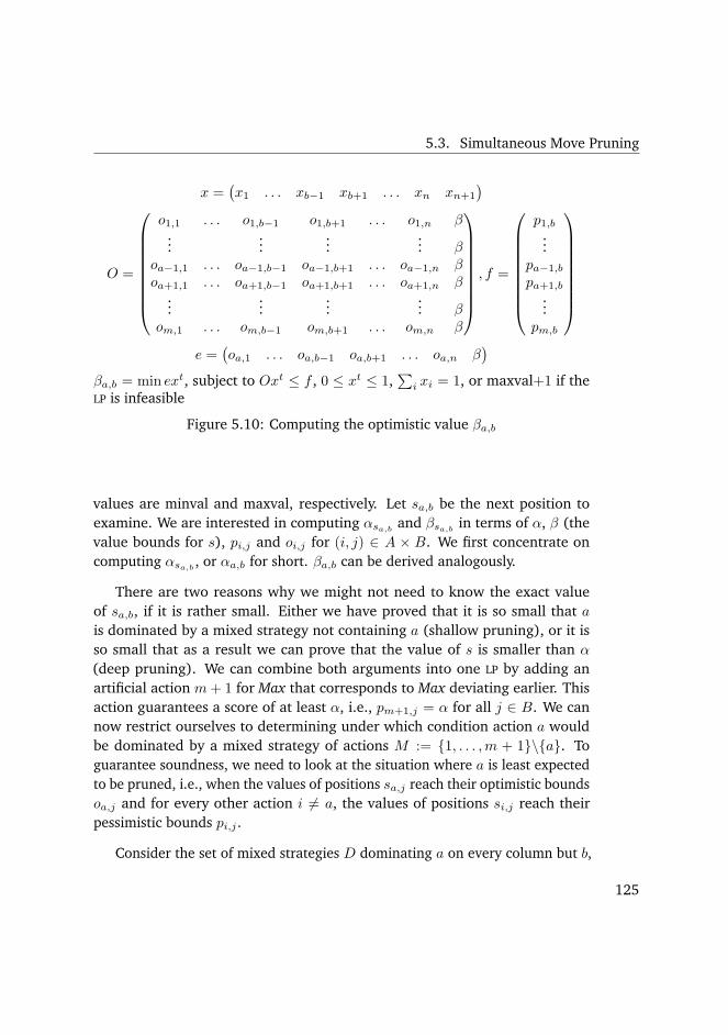
5.3. Simultaneous Move Pruning
x =(x1 . . . xb−1 xb+1 . . . xn xn+1
)
O =
o1,1 . . . o1,b−1 o1,b+1 . . . o1,n β...
......
... βoa−1,1 . . . oa−1,b−1 oa−1,b+1 . . . oa−1,n βoa+1,1 . . . oa+1,b−1 oa+1,b+1 . . . oa+1,n β
......
...... β
om,1 . . . om,b−1 om,b+1 . . . om,n β
, f =
p1,b...
pa−1,b
pa+1,b
...pm,b
e =(oa,1 . . . oa,b−1 oa,b+1 . . . oa,n β
)
βa,b = min ext, subject to Oxt ≤ f , 0 ≤ xt ≤ 1,∑
i xi = 1, or maxval+1 if theLP is infeasible
Figure 5.10: Computing the optimistic value βa,b
values are minval and maxval, respectively. Let sa,b be the next position to
examine. We are interested in computing αsa,band βsa,b
in terms of α, β (the
value bounds for s), pi,j and oi,j for (i, j) ∈ A × B. We first concentrate on
computing αsa,b, or αa,b for short. βa,b can be derived analogously.
There are two reasons why we might not need to know the exact value
of sa,b, if it is rather small. Either we have proved that it is so small that a
is dominated by a mixed strategy not containing a (shallow pruning), or it is
so small that as a result we can prove that the value of s is smaller than α
(deep pruning). We can combine both arguments into one LP by adding an
artificial action m+ 1 for Max that corresponds to Max deviating earlier. This
action guarantees a score of at least α, i.e., pm+1,j = α for all j ∈ B. We can
now restrict ourselves to determining under which condition action a would
be dominated by a mixed strategy of actions M := {1, . . . ,m + 1}\{a}. To
guarantee soundness, we need to look at the situation where a is least expected
to be pruned, i.e., when the values of positions sa,j reach their optimistic bounds
oa,j and for every other action i 6= a, the values of positions si,j reach their
pessimistic bounds pi,j .
Consider the set of mixed strategies D dominating a on every column but b,
125

5. GAMES WITH SIMULTANEOUS MOVES
i.e.,
D = {x ∈ Rm≥0 |
∑
i
xi = 1, ∀j 6= b :∑
i∈M
xipi,j ≥ oa,j} (5.2)
Action a is dominated if and only if a is dominated on column b by a strategy
in D. I.e., action a is dominated if and only if value v of sa,b satisfies:
∃x ∈ D :∑
i∈M
xipi,b ≥ v (5.3)
If D is non-empty, to have the tightest αa,b possible, we maximize over such
values:
αa,b = maxx∈D
∑
i∈M
xipi,b (5.4)
Otherwise, if D is empty, sa,b can’t be bound from below and we set αa,b =
minval.
This process can be directly translated into the LP presented in Figure 5.9.
Similarly, the bound βsa,bis defined as the objective value of the LP shown in
Figure 5.10.
5.3.3 Main Algorithm
Algorithm 10 describes how our simultaneous move pruning can be incorporated
in a depth-first search algorithm by looping through all joint action pairs first
checking trivial exit conditions and if these fail, proceeding with computing
optimistic and pessimistic bounds for the entry in questions, and then recursively
computing the entry value. We call this procedure Simultaneous Move Alpha-
Beta (SMAB) Search.
Theorem 8. When SMAB is called with s, α, β and α < β . . .
1. . . . it runs in weakly polynomial time in the size of the game tree rooted in s.
2. . . . and returns v ≤ α, then value(s) ≤ v.
3. . . . and returns v ≥ β, then value(s) ≥ v.
4. . . . and returns α < v < β, then value(s) = v.
Proof sketch.
126

5.3. Simultaneous Move Pruning
Algorithm 10: Pseudo-code for simultaneous move Alpha-Beta search.Function Nash(X) computes the Nash equilibrium value of normal-formgame payoff matrix X for row player Max.
SMAB(state s, lower bound α, upper bound β)if s ∈ F then return σ(s)else
pi,j ← b for i ∈ L1(s), j ∈ L2(s)oi,j ← a for i ∈ L1(s), j ∈ L2(s)Let P denote the matrix formed by all pi,jLet O denote the matrix formed by all oi,jforeach (a, b) ∈ L1(s)× L2(s) do
if row a and column b are not dominated thenLet αa,b as defined in Fig. 5.9 restricted to non-dominatedactionsLet βa,b as defined in Fig. 5.10 restricted to non-dominatedactionssa,b ← the state reached after applying (a, b) to sif αa,b ≥ βa,b then
va,b ← SMAB(sa,b, αa,b, αa,b + ǫ)if va,b ≤ αa,b then a is dominatedelse b is dominated
elseva,b ← SMAB(sa,b, αa,b, βa,b)if va,b ≤ αa,b then a is dominatedelse if va,b ≥ βa,b then b is dominatedelse pa,b ← va,b; oa,b ← va,b
return Nash(P restricted to non-dominated actions)
1.: Weakly polynomial run-time in the sub-tree size can be shown by induction
on the tree height using the fact that LPs can be solved by interior point
methods in weakly polynomial time.
2.,3.,4.: Induction on tree height h. For h = 0, SMAB immediately returns the
true value. Thus, properties 2.-4. hold. Now we assume they hold for all
heights h ≤ k and s has height k + 1 and proceed with an induction on
the number of inner loop iterations claiming that P and O are correctly
127

5. GAMES WITH SIMULTANEOUS MOVES
updated in each step (using the derivations in the previous subsection
and the main induction hypothesis) and if line 28 is reached, properties
2.-4. hold.
5.3.4 Ordering Move Pairs
Heuristics can be used to initialize (pi,j , oi,j), given that they have the admissi-
bility property with regards to the bound they are applied to. As an example, we
might in some game know from the material strength on the board in some state
that we are guaranteed at least a draw, allowing us to initialize the pessimistic
value to a draw. Similarly, we should be able to set the optimistic value to a
draw if the opponent is equally up in material.
Additionally, the order in which the pairs (a, b) will be visited in Algorithm 10
can dramatically affect the amount of pruning. This problem can be decomposed
into two parts. Move ordering in which the individual moves are ordered and
cell ordering in which the joint moves are ordered based on the order of the
individual moves. Formally, move ordering means endowing the sets A and
B with total orders <A and <B and cell ordering is the construction of a total
order for A×B based on <A and <B . For instance, the lexicographical ordering
is a possible cell ordering: (a1, b1) will be explored before (a2, b2) iff a1 <A a2or a1 = a2 and b1 < b2. We will discuss heuristic cell orderings in the next
section.
5.4 Fast approximate search for combat games
In the previous section we discussed multiple game transformations that would
allow us to find solutions by using backward induction. However, when playing
RTS games the real-time constraints are harsh. Often, decisions must be made
during a single simulation frame, which can be 50 ms or shorter. Therefore,
computing optimal moves is impossible for all but the smallest settings and we
need to settle for approximate solutions: we trade optimality for speed and
hope that the algorithms we propose defeat the state of the art AI systems for
combat games.
128

5.4. Fast approximate search for combat games
The common approach is to declare nodes to be leaf nodes once a certain
depth limit is reached. In leaf nodes Max’s utility is then estimated by calling an
evaluation function, and this value is propagated up the tree like true terminal
node utilities.
In the following subsections we will first adapt the Alpha-Beta search algo-
rithm to combat games by handling durative moves explicitly and then present
a series of previously known and new evaluation functions.
5.4.1 Scripted behaviors
The simplest approach, and the one most commonly used in video game AI
systems, is to define static behaviors via AI scripts. Their main advantage is
computation speed, but they often lack foresight, which makes them vulnerable
against search-based methods, as we will see in Section 5.5, where we will
evaluate the following simple combat AI scripts:
• The Random strategy picks legal moves with uniform probability.
• Using the Attack-Closest strategy units will attack the closest opponent
unit within weapon’s range if it can currently fire. Otherwise, if it is
within range of an enemy but is reloading, it will wait in-place until it has
reloaded. If it is not in range of any enemy, it will move toward the closest
enemy a fixed distance.
• The Attack-Weakest strategy is similar to Attack-Closest, except units attack
an opponent unit with the lowest hp within range when able.
• Using the Kiting strategy is similar to Attack-Closest, except it will move a
fixed distance away from the closest enemy when it is unable to fire.
The Attack-Closest script was used in second-place entry UAlbertaBot in the
2010 AIIDE STARCRAFT AI competition, whereas Skynet, the winning entry, used
a behavior similar to Kiting. The scripts presented so far are quite basic but we
can add a few smarter ones to our set of scripts to test.
• The Attack-Value strategy is similar to Attack-Closest, except units attack
an opponent unit u with the highest dpf(u)/hp(u) value within range
when able. This choice leads to optimal play in 1 vs. n scenarios [52].
129

5. GAMES WITH SIMULTANEOUS MOVES
• The No Overkill/Attack Value (NOK-AV) strategy is similar to Attack-Value,
except units will not attack an enemy unit which has been assigned lethal
damage this round. It will instead choose the next priority target, or wait
if one does not exist.
• Using the Kiting-AV strategy is similar to Kiting, except it will choose an
attack target similar to Attack-Value.
Most scripts we described make decisions on an individual unit basis, with
some creating the illusion of unit collaboration (by concentrating fire on closest,
weakest, or most-valuable units). NOK-AV is the only script in our set that exhibits
true collaborative behaviour by sharing information about unit targeting.
5.4.2 Alpha-Beta Search with Durative Moves
Consider Figure 5.11 which displays a typical path in the sequentialized game
tree. Because of the weapon cooldown and the space granularity, battle games
exhibit numerous durative moves. Indeed, there are many time steps where the
only move for a player is just pass, since all the units are currently unable to
perform an action. Thus, non-trivial decision points for players do not occur on
every frame.
Given a player p in a state s, define the next time where p is next able to
do a non-pass move by τ(s, p) = minu∈s.Up(u.ta, u.tm). Note that for any time
step t such that s.t < t < min(τ(s,Max), τ(s,Min)), players cannot perform
any move but pass. It is therefore possible to shortcut many trivial decision
points between s.t and min(τ(s,Max), τ(s,Min)).
Assume an evaluation function has been picked, and remaining simultaneous
choices are sequentialized as suggested above. It is then possible to adapt the
Alpha-Beta algorithm to take advantage of durative moves as presented in
Algorithm 11
We use the terminal(s, d) function to decide when to call the evaluation
function. It is parametrized by a maximal depth dmax and a maximal time tmax
and return “true” if s is a terminal position or d ≥ dmax or s.t ≥ tmax.
The third argument to the ABCD algorithm is used to handle the delayed
action effect mechanism for sequentialized simultaneous moves. If the state
does not correspond to a simultaneous decision, m0 holds a dummy value ∅.
130

5.4. Fast approximate search for combat games
t0
t1
t2
t3
t4
t5
t6
Time Action Sequences Path in Game Tree
M1
M2
M3
M4
m1
m2
m3
m4
m5
(M1,m1)
M2
m2
(M3,m3)
m4
(M4,m5)
Max node Min node Nash node
Figure 5.11: Durations
Otherwise, we apply the effects of m0 after move m is generated because m0
should not affect the generation of the complementary moves.
5.4.3 Evaluation Functions
A straight-forward evaluation function for combat games is the hitpoint-total
differential (Equation 5.5) which, however, does not take into account other
unit properties, such as damage values and cooldown periods.
e(s) =∑
u∈U1
hp(u)−∑
u∈U2
hp(u) (5.5)
Kovarsky and Buro (2005) propose an evaluation based on the life-time damage
a unit can inflict, which is proportional to its hp times its damage-per-frame
ratio:
131

5. GAMES WITH SIMULTANEOUS MOVES
Algorithm 11: Alpha-Beta (Considering Durations) (ABCD)
abcd(s, d, m0, α, β)if computationTime.elapsed then return timeout
else if s ∈ F or d = 0 then return ζ(s)τ ← s.playerToMove(policy)while m← s.nextMove(τ) do
if s.bothCanMove and m0 = ∅ and d 6= 1 thenv ←abcd(s, d− 1, m, α, β)
elses′ ← sif m0 6= ∅ then s′.doMove(m0)s′.doMove(m)v ←abcd(s′, d− 1, ∅, α, β)
if τ = Max and v > α then α← vif τ = Min and v < β then β ← vif α ≥ β then break
if τ = Max then return αelse return β
dpf(u) =damage(w(u))
cooldown(w(u))(5.6)
LTD(s) =∑
u∈U1
hp(u) · dpf(u)−∑
u∈U2
hp(u) · dpf(u) (5.7)
A second related evaluation function propose favours uniform hp distribu-
tions [79]:
LTD2(s) =∑
u∈U1
√
hp(u) · dpf(u)−∑
u∈U2
√
hp(u) · dpf(u) (5.8)
While these evaluation functions are exact for terminal positions, they can
be drastically inaccurate for many non-terminal positions. To improve state
evaluation by also taking other unit properties such as speed and weapon range
into account, we can try to simulate a game and use the outcome as an estimate
of the utility of its starting position. This idea is known as performing a playout
132

5.5. Experiments
in game tree search and is actually a fundamental part of MCTS algorithms which
have revolutionized computer GO [40]. However, there are differences between
the playouts we advocate for combat games and previous work on GO and HEX:
the playout policies we use here are deterministic and we are not using MCTS or
a best-first search algorithm, but rather depth-first search.
5.4.4 Move Ordering
It is well-known in the game AI research community that a good move ordering
fosters the performance of the Alpha-Beta algorithm. When Transposition
Tables (TTs) and iterative deepening are used, reusing previous search results
can improve the move ordering. Suppose a position p needs to be searched
at depth d and was already searched at depth d′. If d ≤ d′, the value of the
previous search is sufficiently accurate and there is no need for an additional
search on p. Otherwise, a deeper search is needed, but we can explore the
previously found best move first and hope for more pruning.
When no TT information is available, we can use scripted strategies to
suggest moves. We call this new heuristic scripted move ordering. Note that
this heuristic could also be used in standard sequential games like CHESS. We
believe the reason it has not been investigated closely in those contexts is the
lack of high quality scripted strategies.
5.5 Experiments
5.5.1 Solving GOOFSPIEL
As a test case we implemented SMAB pruning for the game of GOOFSPIEL. The
following experimental results were obtained running OCaml 3.11.2, g++ 4.5.2,
and the glpk 4.43 LP-solver under Ubuntu on a laptop with Intel T3400 CPU at
2.2 GHz.
The game GOOFSPIEL [117, 142] uses cards in three suits. In the version
we use, each player has all the cards of a single suit and the remaining suit is
stacked on the table face up in a pre-defined order. On each turn both players
simultaneously play a card from their hand and the higher card wins its player
the top card from the table. If the played cards are of equal value the table card
is discarded. When all cards have been played the winner is the player whose
133

5. GAMES WITH SIMULTANEOUS MOVES
1 2 3 4 5
6 10 11 12 13
7 14 17 18 19
8 15 20 22 23
9 16 21 24 25
Figure 5.12: L-shaped cell ordering for 5× 5 matrices.
accumulated table cards sum up to a higher value. We used games with various
number of cards per suit to monitor how the pruning efficiency develops with
increasing game-tree sizes.
We use a cell ordering that strives to keep a balance between the number of
rows filled and the number of columns filled. We call it L-shaped and it can be
seen as the lexicographical ordering over tuples (min{a, b}, a, b). Its application
to 5×5 matrix is described in Figure 5.12. In all of our preliminary experiments,
the L-shaped ordering proved to lead to earlier and more pruning than the
natural lexicographical orderings.
To save some calculations, it is possible to skip the LP computations for some
cells and directly set the corresponding α and β bounds to (b− 1) and (a+ 1),
respectively. On the one hand, if the computed bounds wouldn’t have enabled
much pruning, then using the default bounds instead allows to save some time.
On the other hand, if too many bounds are loose, there will be superfluous
computations in prunable subtrees.
To express this tradeoff, we introduce the early bound skipping heuristic. This
heuristic is parameterized by an integer s and consists in skipping the LP-based
computations of the α and β bounds as long as the matrix does not have at least
s rows and s columns completely filled. For instance, if we use this heuristic
together with the L-shaped ordering on a 5× 5 matrix with parameter s = 1, no
LP computation takes place for the bounds of the first 9 cells.
In our backward induction implementation that recursively solves subgames
in depth-first fashion, we used one LP call per non-terminal node expansion.
Table 5.3 shows the number of non-terminal node expansions/LP calls, the total
134

5.5. Experiments
Table 5.3: Solving GOOFSPIEL with backward induction.
size nodes (= LP calls) total time LP time
4 109 0.008 0.0045 1926 0.188 0.1366 58173 5.588 4.2007 2578710 247.159 184.616
Table 5.4: Solving GOOFSPIEL with a sequence form solver.
size memory time
4 8 MB < 1 s5 43 MB 152 s6 > 2 GB > 177 s
Table 5.5: Solving GOOFSPIEL with SMAB.
size nodes LP calls total time LP time s
4 55 265 0.020 0.016 04 59 171 0.012 0.012 14 70 147 0.012 0.012 2
5 516 2794 0.216 0.148 05 630 1897 0.168 0.128 15 1003 1919 0.184 0.152 2
6 13560 74700 5.900 4.568 06 18212 55462 4.980 3.852 16 30575 57335 5.536 4.192 2
7 757699 4074729 324.352 245.295 07 949521 2857133 259.716 197.700 17 1380564 2498366 241.735 182.463 27 1734798 2452624 237.903 177.411 37 1881065 2583307 253.476 188.276 4
135

5. GAMES WITH SIMULTANEOUS MOVES
time spent running the algorithm, and the time spent specifically solving LPs.
Table 5.5 shows the same information for SMAB using L-shaped ordering and
early bound skipping parameterized by s. This table has separate columns for
the number of non-terminal node expansions and the number of calls to the LP
solver as they are not equal in the case of SMAB.
Table 5.4 shows the memory and time needed to solve GOOFSPIEL using a se-
quence form solver based on based on [77]. The algorithm needs a huge amount
of memory to solve even a moderate size instance of GOOFSPIEL. The backward
induction and the SMAB implementations, on the contrary, never needed more
than 60 MB of memory. This difference is expected as the backward induction
and SMAB are depth-first search algorithms solving hundreds of thousands of
relatively small LPs while the sequence form algorithm solves a single large LP.
5.5.2 Real-time Strategy games
We implemented the proposed combat model, the scripted strategies, the new
ABCD algorithm, and various tree transformations. We then ran experiments to
measure 1) the influence of the suggested search enhancements for determining
the best search configuration, and 2) the real-time exploitability of scripted
strategies.
Because of time constraints, we were only able to test the following tree
transformations: Alt, Alt’, and RAB’, where Alt’ in simultaneous move nodes
selects the player that acted last, and RAB’ selects the player to move like RAB,
but only completes one Alpha-Beta search.
Setup The combat scenarios we used for the experiments involved equally
sized armies of n versus n units, where n varied from 2 to 8. 1 versus 1 scenarios
were omitted due to over 95% of them resulting in draws. Four different army
types were constructed to mimic various combat scenarios. These armies were:
Marine Only, Marine + Zergling, Dragoon + Zealot, and Dragoon + Marine.
Armies consisted of all possible combinations of the listed unit type with up
to 4 of each, for a maximum army size of 8 units. Each unit in the army was
given to player Max at random starting position (x, y) within 256 pixels of the
origin, and to player Minat position (−x,−y), which guaranteed symmetric
start locations about the origin. Once combat began, units were allowed to
136

5.5. Experiments
move infinitely within the plane. Unit movement was limited to up, down, left,
right at 15 pixel increments, which is equal to the smallest attack range of any
unit in our tests.
These settings ensured that the Nash value of the starting position was
always 0.5. If the battle did not end in one player being eliminated after 500
actions, the simulation was halted and the final state evaluated with LTD. For
instance, in a match between a player p1 and an opponent p2, we would count
the number of wins by p1, w, and number of draws, d, over n games and
compute r = (w + d/2)/n. Both players perform equally well in this match if
r ≈ 0.5.
As the 2011 STARCRAFT AI Competition allowed for 50 ms of processing
per game logic frame, we gave each search episode a time limit of 5 ms. This
simulates the real-time nature of RTS combat, while leaving plenty of time (45
ms) for other processing which may have been needed for other computations.
Experiments were run single-threaded on an Intel Core i7 2.67 GHz CPU
with 24 GB of 1600 MHz DDR3 RAM using the Windows 7 64 bit operating
system and Visual C++ 2010. A transposition table of 5 million entries (20
bytes each) was used. Due to the depth-first search nature of the algorithm,
very little additional memory is required to facilitate search. Each result table
entry is the result of playing 365 games, each with random symmetric starting
positions.
Influence of the Search Settings To measure the impact of certain search
parameters, we perform experiments using two methods of comparison. The first
method plays static scripted opponents vs. ABCD with various settings, which are
then compared. The second method plays ABCD vs. ABCD with different settings
for each player.
We start by studying the influence of the evaluation function selection on
the search performance (see Section 5.4.3). Preliminary experiments revealed
that using NOK-AV for the playouts was significantly better than using any of the
other scripted strategies. The playout-based evaluation function will therefore
always use the NOK-AV script.
We now present the performance of various settings for the search against
script-based opponents (Table 5.6) and search-based opponents (Table 5.7).
In Table 5.6, the Alt sequentialization is used among the first three settings
137
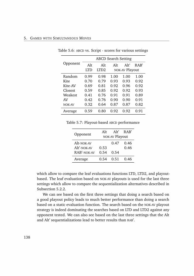
5. GAMES WITH SIMULTANEOUS MOVES
Table 5.6: ABCD vs. Script - scores for various settings
OpponentABCD Search Setting
Alt Alt Alt Alt’ RAB’LTD LTD2 NOK-AV Playout
Random 0.99 0.98 1.00 1.00 1.00Kite 0.70 0.79 0.93 0.93 0.92Kite-AV 0.69 0.81 0.92 0.96 0.92Closest 0.59 0.85 0.92 0.92 0.93Weakest 0.41 0.76 0.91 0.91 0.89AV 0.42 0.76 0.90 0.90 0.91NOK-AV 0.32 0.64 0.87 0.87 0.82
Average 0.59 0.80 0.92 0.92 0.91
Table 5.7: Playout-based ABCD performance
OpponentAlt Alt’ RAB’NOK-AV Playout
Alt-NOK-AV 0.47 0.46Alt’-NOK-AV 0.53 0.46RAB’-NOK-AV 0.54 0.54
Average 0.54 0.51 0.46
which allow to compare the leaf evaluations functions LTD, LTD2, and playout-
based. The leaf evaluation based on NOK-AV playouts is used for the last three
settings which allow to compare the sequentialization alternatives described in
Subsection 5.2.2.
We can see based on the first three settings that doing a search based on
a good playout policy leads to much better performance than doing a search
based on a static evaluation function. The search based on the NOK-AV playout
strategy is indeed dominating the searches based on LTD and LTD2 against any
opponent tested. We can also see based on the last three settings that the Alt
and Alt’ sequentializations lead to better results than RAB’.
138

5.6. Conclusion and Future Work
Table 5.8: Real-time exploitability of scripted strategies.
Random Weakest Closest AV Kiter Kite-AV NOK-AV
1.00 0.98 0.98 0.98 0.97 0.97 0.95
Estimating the Quality of Scripts The quality of scripted strategies can be
measured in at least two ways: the simplest approach is to run the script
against multiple opponents and average the results. To this end, we can use
the data presented in Table 5.6 to conclude that NOK-AV is the best script in
our set. Alternatively, we can measure the exploitability of scripted strategies
by determining the score a theoretically optimal best-response-strategy would
achieve against the script. However, such strategies are hard to compute in
general. Looking forward to modelling and exploiting opponents, we would
like to approximate best-response strategies quickly, possibly within one game
simulation frame. This can be accomplished by replacing one player in ABCD
by the script in question and then run ABCD to find approximate best-response
moves. The obtained tournament result we call the real-time exploitability of
the given script. It constitutes a lower bound (in expectation) on the true
exploitability and tells us about the risk of being exploited by an adaptive player.
Table 5.8 lists the real-time exploitability of various scripted strategies. Again,
the NOK-AV strategy prevails, but the high value suggests that there is room for
improvement.
5.6 Conclusion and Future Work
We have shown that it is possible to extend Alpha-Beta pruning to include
simultaneous move games and that our SMAB pruning procedure can reduce
the node count and run-time when solving non-trivial games. In the reported
experiments we used a fixed move ordering and a fixed cell ordering. The
results show a considerable drop in node expansions, even though not nearly as
much as with Alpha-Beta in the sequential setting, but certainly enough to be
very promising. Still, this threshold is not high and with increasing game size
the run-time appears to be increasingly improving. The pruning criterion we
propose is sound, but it only allows us to prune provably dominated actions.
139
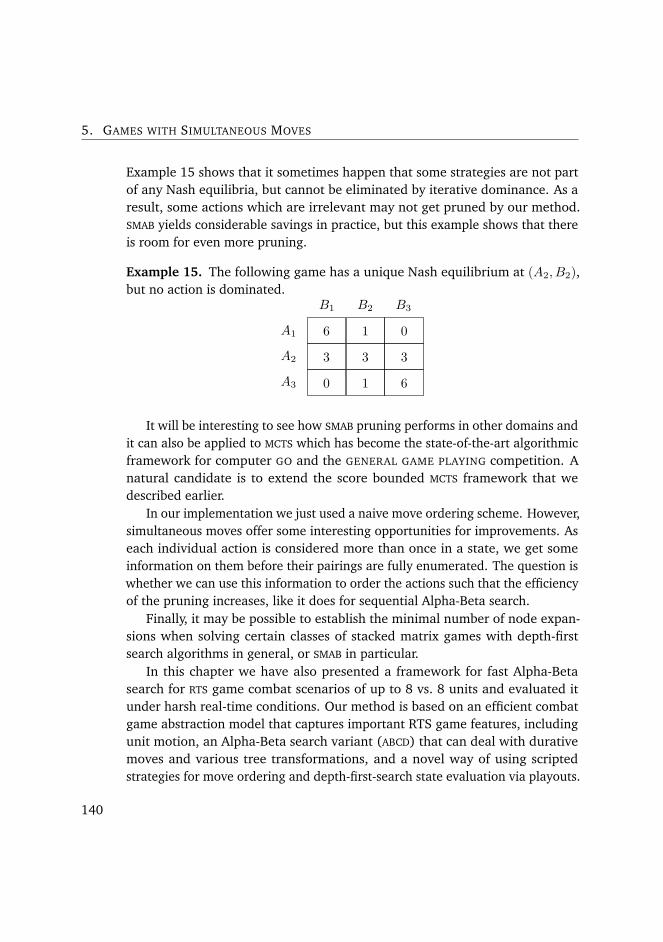
5. GAMES WITH SIMULTANEOUS MOVES
Example 15 shows that it sometimes happen that some strategies are not part
of any Nash equilibria, but cannot be eliminated by iterative dominance. As a
result, some actions which are irrelevant may not get pruned by our method.
SMAB yields considerable savings in practice, but this example shows that there
is room for even more pruning.
Example 15. The following game has a unique Nash equilibrium at (A2, B2),
but no action is dominated.
6 1 0
3 3 3
0 1 6
A1
A2
A3
B1 B2 B3
It will be interesting to see how SMAB pruning performs in other domains and
it can also be applied to MCTS which has become the state-of-the-art algorithmic
framework for computer GO and the GENERAL GAME PLAYING competition. A
natural candidate is to extend the score bounded MCTS framework that we
described earlier.
In our implementation we just used a naive move ordering scheme. However,
simultaneous moves offer some interesting opportunities for improvements. As
each individual action is considered more than once in a state, we get some
information on them before their pairings are fully enumerated. The question is
whether we can use this information to order the actions such that the efficiency
of the pruning increases, like it does for sequential Alpha-Beta search.
Finally, it may be possible to establish the minimal number of node expan-
sions when solving certain classes of stacked matrix games with depth-first
search algorithms in general, or SMAB in particular.
In this chapter we have also presented a framework for fast Alpha-Beta
search for RTS game combat scenarios of up to 8 vs. 8 units and evaluated it
under harsh real-time conditions. Our method is based on an efficient combat
game abstraction model that captures important RTS game features, including
unit motion, an Alpha-Beta search variant (ABCD) that can deal with durative
moves and various tree transformations, and a novel way of using scripted
strategies for move ordering and depth-first-search state evaluation via playouts.
140

5.6. Conclusion and Future Work
The experimental results are encouraging. Our search, when using only 5 ms per
episode, defeats standard AI scripts as well as more advanced scripts that exhibit
kiting behaviour and minimize overkill. The prospect of opponent modelling for
exploiting scripted opponents is even greater: the practical exploitability results
indicate large win margins best-response ABCD can achieve if the opponent
executes any of the tested combat scripts.
The ultimate goal of this line of research is to handle larger combat scenarios
with more than 20 units on each side in real-time. The enormous state and move
complexity, however, prevents us from applying heuristic search directly, and we
therefore will have to find spatial and unit group abstractions that reduce the
size of the state space so that heuristic search can produce meaningful results
in real-time. Balla and Fern (2009) present initial research in this direction, but
their Upper Confidence bound for Trees (UCT)-based solution is rather slow and
depends on pre-assigned unit groups.
Our next steps will be to integrate ABCD search into a STARCRAFT AI competi-
tion entry to gauge its performance against previous year’s participants, to refine
our combat model if needed, to add opponent modelling and best-response-ABCD
to counter inferred opponent combat policies, and then to tackle more complex
combat scenarios.
141


6 Conclusion
In this thesis, we have proposed a generic BFS framework for two-outcome
games and we have adapted and extended it to multi-outcome games and MMLK
model checking. This gives access to generalizations of PNS and MCTS Solver for
multi-outcome games and for MMLK model checking. An attractive direction for
future work would be to express a similar BFS framework for other classes of
multi-agent systems. Candidate classes comprise simple stochastic games or
competitive Markov Decision Processes (MDPs) [35, 36, 44], and stacked-matrix
games as defined in Chapter 5.
We have generalized alpha-beta pruning to stacked-matrix games. Develop-
ing a safe pruning criterion for the general class of Multi-Agent Environment
as defined by Schiffel and Thielscher [138] seems accessible now, as it only
requires combining our approach with that of Sturtevant for non-zero and
multi-player games [147, 148].
The approach that we have taken in Chapter 2, 3, and 5 make an implicit
closed-world assumption: we assumed that computing the game-theoretic value
of a position was all the information we could ever need. Combinatorial Game
Theory goes a step further as it considers it possible that the game could be just
a small part of a bigger game [1]. In such a setting, it is possibe that a player
plays twice in a row in a subgame if the opponent plays in another subgame. As
a result, there is more information to extract from a position than its minimax
value. The maximum amount of information a position contains is called the
canonical form and algorithms have been developed to compute the canonical
form of any two-player combinatorial game.
However, these algorithms are quite slow and sometimes spend time com-
143

6. CONCLUSION
puting redundant or useless information. Providing a safe pruning mechanism a
la alpha-beta would certainly enable much faster computations in certain cases.
We can also envision adapting the BFS framework presented in this thesis to the
computation of canonical forms in combinatorial game theory.
144

A Combat game abstract model
To fully simulate RTS game combat, our model is comprised of three main
components: states, units, and moves.
State s = 〈t, U1, U2〉
• Current game time t
• Sets of units Ui under control of player i
Unit u = 〈p, hp, ta, tm, v, w〉
• Position p = (x, y) in R2
• Current hit points hp
• Time step when unit can next attack ta, or move tm
• Maximum unit velocity v
• Weapon properties w = 〈damage, cooldown〉
Move m = {a0, . . . , ak}which is a combination of unit actions ai = 〈u, type, target, t〉,with
• Unit u to perform this action
• The type type of action to be performed:
Attack unit target
Move u to position target
Wait until time t
145

A. COMBAT GAME ABSTRACT MODEL
Given a state s containing unit u, we generate legal unit actions as follows:
if u.ta ≤ s.t then u may attack any target in its range, if u.tm ≤ s.t then u may
move in any legal direction, if u.tm ≤ s.t < u.ta then u may wait until u.ta. If
both u.ta and u.tm are > s.t then a unit is said to have no legal actions. A legal
player move is then a set of all combinations of one legal unit action from each
unit a player controls.
Unlike strict alternating move games like chess, our model’s moves have
durations based on individual unit properties, so either player (or both) may
be able to move at a given state. We define the player to move next as the one
which contains the unit with the minimum time for which it can attack or move.
While the mathematical model we propose does not exactly match the
combat mechanics of STARCRAFT it captures essential features. Because we
don’t have access to STARCRAFT’s source code, we can only try to infer missing
features based on game play observations:
• no spell casting (e.g., immobilization, area effects)
• no hit point or shield regeneration
• no travel time for projectiles
• no unit collisions
• no unit acceleration, deceleration or turning
• no fog of war
Quite a few STARCRAFT AI competition entries are designed with a strong focus
on early game play (rushing). For those programs some of the listed limitations,
such as single weapons and spell casting, are immaterial because they become
important only in later game phases. The utility of adding others, such as
dealing with unit collisions and acceleration, will have to be determined once
our search technique becomes adopted.
146

Bibliography
[1] Michael H. Albert, Richard J. Nowakowski, and David Wolfe. Lessons in
play: an introduction to combinatorial game theory. AK Peters Ltd, 2007.
[2] Louis Victor Allis. A knowledge-based approach of connect-four the
game is solved: White wins. Master’s thesis, Vrije Universitat Amsterdam,
Amsterdam, The Netherlands, October 1988.
[3] Louis Victor Allis. Searching for Solutions in Games an Artificial Intelli-
gence. PhD thesis, Vrije Universitat Amsterdam, Department of Computer
Science, Rijksuniversiteit Limburg, 1994.
[4] Louis Victor Allis, M. van der Meulen, and H. Jaap van den Herik. Proof-
Number Search. Artificial Intelligence, 66(1):91–124, 1994.
[5] Louis Victor Allis, H. Jaap van den Herik, and M. P. H. Huntjens. Go-
Moku solved by new search techniques. Computational Intelligence, 12:
7–23, 1996.
[6] Rajeev Alur, Thomas A. Henzinger, and Orna Kupferman. Alternating-
time temporal logic. Journal of the ACM, 49(5):672–713, 2002.
[7] Broderick Arneson, Ryan B. Hayward, and Philip Henderson. Monte Carlo
tree search in hex. IEEE Transactions on Computational Intelligence and
AI in Games, 2(4):251–258, 2010. doi: 10.1109/TCIAIG.2010.2067212.
[8] Broderick Arneson, Ryan B. Hayward, and Philip Henderson. Solving
hex: Beyond humans. In H. Jaap van den Herik, Hiroyuki Iida, and Aske
147
BIBLIOGRAPHY
Plaat, editors, Computers and Games, volume 6515 of Lecture Notes in
Computer Science, pages 1–10. Springer, Berlin Heidelberg, 2011. ISBN
978-3-642-17927-3. doi: 10.1007/978-3-642-17928-0 1.
[9] Peter Auer, Nicolo Cesa-Bianchi, and Paul Fischer. Finite-time analysis
of the multiarmed bandit problem. Machine learning, 47(2):235–256,
2002.
[10] David Auger and Olivier Teytaud. The frontier of decidability in partially
observable games. International Journal on Foundations of Computer
Science, 23(7):1439–1450, 2012. doi: 10.1142/S0129054112400576.
[11] Christel Baier and Joost-Pieter Katoen. Principles of model checking. The
MIT Press, April 2008. ISBN 026202649X.
[12] Radha-Krishna Balla and Alan Fern. UCT for tactical assault planning in
real-time strategy games. In Boutilier [17], pages 40–45.
[13] Bruce W. Ballard. The *-minimax search procedure for trees containing
chance nodes. Artificial Intelligence, 21(3):327–350, 1983.
[14] Patrick Blackburn, Maarten De Rijke, and Yde Venema. Modal Logic,
volume 53. Cambridge University Press, 2001.
[15] Edouard Bonnet, Florian Jamain, and Abdallah Saffidine. Havannah
and Twixt are PSPACE-complete. In 8th International Conference on
Computers and Games (CG). Yokohama, Japan, August 2013.
[16] Edouard Bonnet, Florian Jamain, and Abdallah Saffidine. On the com-
plexity of trick-taking card games. In 23rd International Joint Conference
on Artificial Intelligence (IJCAI), Beijing, China, August 2013. AAAI Press.
[17] Craig Boutilier, editor. IJCAI 2009, Proceedings of the 21st International
Joint Conference on Artificial Intelligence, Pasadena, California, USA, July
2009.
[18] Dennis M. Breuker, Jos W.H.M. Uiterwijk, and H. Jaap van den Herik.
Solving 8×8 domineering. Theoretical Computer Science, 230(1-2):195–
206, 2000. doi: 10.1016/S0304-3975(99)00082-1.
148

Bibliography
[19] Dennis Michel Breuker. Memory versus Search in Games. PhD thesis,
Universiteit Maastricht, 1998.
[20] Cameron Browne, Edward Powley, Daniel Whitehouse, Simon Lucas,
Peter Cowling, Philipp Rohlfshagen, Stephen Tavener, Diego Perez,
Spyridon Samothrakis, and Simon Colton. A survey of Monte Carlo
tree search methods. Computational Intelligence and AI in Games,
IEEE Transactions on, 4(1):1–43, March 2012. ISSN 1943-068X. doi:
10.1109/TCIAIG.2012.2186810.
[21] Michael Buro. Solving the Oshi-Zumo game. In H. Jaap van den Herik,
Hiroyuki Iida, and Ernst A. Heinz, editors, 10th International Conference
on Advances in Computer Games, Many Games, Many Challenges, volume
263 of IFIP, pages 361–366, Graz, Austria, November 2003. Kluwer. ISBN
1-4020-7709-2.
[22] Michael Buro, Jeffrey R. Long, Timothy Furtak, and Nathan R. Sturtevant.
Improving state evaluation, inference, and search in trick-based card
games. In Boutilier [17].
[23] Tristan Cazenave. Abstract Proof Search. In T. Anthony Marsland and
Ian Frank, editors, Computers and Games 2000, volume 2063 of Lecture
Notes in Computer Science, pages 39–54. Springer, Berlin / Heidelberg,
2002. ISBN 3-540-43080-6.
[24] Tristan Cazenave and Richard J. Nowakowski. Retrograde analysis of
woodpush. In Games of no chance 4, Banff, Canada, 2011.
[25] Tristan Cazenave and Abdallah Saffidine. Utilisation de la recherche
arborescente Monte-Carlo au Hex. Revue d’Intelligence Artificielle, 23
(2-3):183–202, 2009. doi: 10.3166/ria.23.183-202.
[26] Tristan Cazenave and Abdallah Saffidine. Score bounded Monte-Carlo
tree search. In H. van den Herik, Hiroyuki Iida, and Aske Plaat, editors,
Computers and Games, volume 6515 of Lecture Notes in Computer Science,
pages 93–104. Springer-Verlag, Berlin / Heidelberg, 2011. ISBN 978-3-
642-17927-3. doi: 10.1007/978-3-642-17928-0 9.
149

BIBLIOGRAPHY
[27] Benjamen E. Childs, James H. Brodeur, and Levente Kocsis. Trans-
positions and move groups in Monte Carlo Tree Search. In Philip
Hingston and Luigi Barone, editors, IEEE Symposium on Computa-
tional Intelligence and Games (CIG’08), pages 389–395, 2008. doi:
10.1109/CIG.2008.5035667.
[28] C.-W. Chou, Olivier Teytaud, and Shi-Jin Yen. Revisiting Monte-Carlo
tree search on a normal form game: Nogo. In Cecilia Chio, Stefano
Cagnoni, Carlos Cotta, Marc Ebner, Aniko Ekart, AnnaI. Esparcia-Alcazar,
JuanJ. Merelo, Ferrante Neri, Mike Preuss, Hendrik Richter, Julian To-
gelius, and Georgios N. Yannakakis, editors, Applications of Evolutionary
Computation, volume 6624 of Lecture Notes in Computer Science, pages
73–82. Springer Berlin Heidelberg, 2011. ISBN 978-3-642-20524-8. doi:
10.1007/978-3-642-20525-5 8.
[29] David Churchill and Michael Buro. Build order optimization in starcraft.
In Vadim Bulitko and Mark O. Riedl, editors, 7th AAAI Conference on
Artificial Intelligence and Interactive Digital Entertainment (AIIDE). AAAI
Press, 2011.
[30] David Churchill, Abdallah Saffidine, and Michael Buro. Fast heuristic
search for RTS game combat scenarios. In Mark Riedl and Gita Suk-
thankar, editors, 8th AAAI Conference on Artificial Intelligence and Interac-
tive Digital Entertainment (AIIDE), pages 112–117, Palo Alto, California,
USA, October 2012. AAAI Press.
[31] Edmund M. Clarke, Orna Grumberg, Kenneth L. McMillan, and Xudong
Zhao. Efficient generation of counterexamples and witnesses in symbolic
model checking. In 32nd annual ACM/IEEE Design Automation Conference,
pages 427–432. ACM, 1995. doi: 10.1145/217474.217565.
[32] Edmund M. Clarke, Orna Grumberg, and Doron A. Peled. Model checking.
The MIT Press, 1999.
[33] Edmund M. Clarke, Somesh Jha, Yuan Lu, and Helmut Veith. Tree-like
counterexamples in model checking. In 17th IEEE Symposium on Logic in
Computer Science (LICS), pages 19–29. IEEE Computer Society, 2002.
150
Bibliography
[34] Rance Cleaveland. Tableau-based model checking in the propositional
mu-calculus. Acta Informatica, 27(8):725–747, 1989. doi: 10.1007/
BF00264284.
[35] Anne Condon. The complexity of stochastic games. Information and
Computation, 96(2):203–224, 1992. ISSN 0890-5401. doi: 10.1016/
0890-5401(92)90048-K.
[36] Anne Condon. On algorithms for simple stochastic games. Advances in
computational complexity theory, 13:51–73, 1993.
[37] Vıtor Santos Costa, Luıs Damas, Rogerio Reis, and Ruben Azevedo. YAP
Prolog user’s manual. Universidade do Porto, 2006.
[38] Adrien Couetoux, Jean-Baptiste Hoock, Nataliya Sokolovska, Olivier
Teytaud, and Nicolas Bonnard. Continuous upper confidence trees. In
Carlos A. Coello Coello, editor, Learning and Intelligent Optimization,
pages 433–445. Springer, 2011. doi: 10.1007/978-3-642-25566-3 32.
[39] Adrien Couetoux, Mario Milone, Matyas Brendel, Hassen Doghmen,
Michele Sebag, and Olivier Teytaud. Continuous rapid action value esti-
mates. In Chun-Nan Hsu and Wee Sun Lee, editors, 3rd Asian Conference
on Machine Learning (ACML), volume 20, pages 19–31, 2011.
[40] Remi Coulom. Efficient selectivity and backup operators in Monte-Carlo
tree search. In H. van den Herik, Paolo Ciancarini, and H. Donkers,
editors, Computers and Games, volume 4630 of Lecture Notes in Computer
Science, pages 72–83. Springer, Berlin / Heidelberg, 2007. ISBN 978-3-
540-75537-1. doi: 10.1007/978-3-540-75538-8 7.
[41] Remi Coulom. Computing Elo ratings of move patterns in the game of
Go. ICGA Journal, 30(4):198–208, December 2007.
[42] Joseph C. Culberson and Jonathan Schaeffer. Pattern Databases. Compu-
tational Intelligence, 4(14):318–334, 1998.
[43] Edith Elkind, Jerome Lang, and Abdallah Saffidine. Choosing collectively
optimal sets of alternatives based on the Condorcet criterion. In Toby
Walsh, editor, 22nd International Joint Conference on Artificial Intelligence
151

BIBLIOGRAPHY
(IJCAI), pages 186–191, Barcelona, Spain, July 2011. AAAI Press. ISBN
978-1-57735-516-8.
[44] Kousha Etessami and Mihalis Yannakakis. Recursive markov decision
processes and recursive stochastic games. In Luıs Caires, Giuseppe F.
Italiano, Luıs Monteiro, Catuscia Palamidessi, and Moti Yung, editors,
32nd International Colloquium on Automata, Languages and Programming
(ICALP), volume 3580 of Lecture Notes in Computer Science, pages 891–
903. Springer, 2005. ISBN 3-540-27580-0.
[45] Hugh Everett. Recursive games. Contributions to the Theory of Games III,
39:47–78, 1957.
[46] Timo Ewalds. Playing and solving Havannah. Master’s thesis, University
of Alberta, 2012.
[47] Hilmar Finnsson and Yngvi Bjornsson. Simulation-based approach to
general game playing. In Dieter Fox and Carla P. Gomes, editors, 23rd
AAAI Conference on Artificial Intelligence, pages 259–264. AAAI Press,
July 2008.
[48] Maria Fox and Derek Long. Pddl2.1: An extension to pddl for expressing
temporal planning domains. Journal of Artificial Intelligence Research
(JAIR), 20:61–124, 2003.
[49] Aviezri S. Fraenkel and David Lichtenstein. Computing a perfect strategy
for n× n Chess requires time exponential in n. Journal of Combinatorial
Theory, Series A, 31(2):199–214, 1981.
[50] Aviezri S. Fraenkel, M.R. Garey, David S. Johnson, Thomas J. Schaefer,
and Yaacov Yesha. The complexity of checkers on an n×n board. In 19th
Annual Symposium on Foundations of Computer Science, pages 55–64,
1978. doi: 10.1109/SFCS.1978.36.
[51] Ian Frank and David Basin. Search in games with incomplete information:
A case study using Bridge card play. Artificial Intelligence, 100(1):87–123,
1998.
152

Bibliography
[52] Timothy Furtak and Michael Buro. On the complexity of two-player
attrition games played on graphs. In G. Michael Youngblood and Vadim
Bulitko, editors, 6th AAAI Conference on Artificial Intelligence and In-
teractive Digital Entertainment, AIIDE 2010, Stanford, California, USA,
October 2010.
[53] Timothy Furtak, Masashi Kiyomi, Takeaki Uno, and Michael Buro. Gen-
eralized Amazons is PSPACE-complete. In 19th International Joint Con-
ference on Artificial Intelligence (IJCAI-05), volume 19 of IJCAI-05, pages
132–137, 2005.
[54] Sylvain Gelly and David Silver. Achieving master level play in 9 × 9
computer Go. In Dieter Fox and Carla P. Gomes, editors, 23rd national
conference on Artifical Intelligence (AAAI’08), pages 1537–1540. AAAI
Press, 2008. ISBN 978-1-57735-368-3.
[55] Michael Genesereth and Nathaniel Love. General game playing:
Overview of the AAAI competition. AI Magazine, 26:62–72, 2005.
[56] Andrew Gilpin and Tuomas Sandholm. Lossless abstraction of imperfect
information games. Journal of the ACM, 54(5), 2007. doi: 10.1145/
1284320.1284324.
[57] Matthew L. Ginsberg. GIB: Imperfect information in a computationally
challenging game. Journal of Artificial Intelligence Research (JAIR), 14:
303–358, 2001.
[58] Valentin Goranko and Govert van Drimmelen. Complete axiomatization
and decidability of alternating-time temporal logic. Theoretical Computer
Science, 353(1):93–117, 2006.
[59] Alex Groce and Willem Visser. What went wrong: Explaining counterex-
amples. Model Checking Software, pages 121–136, 2003.
[60] Peter E. Hart, Nils J. Nilsson, and Bertram Raphael. A formal basis for
the heuristic determination of minimum cost paths. IEEE Transactions on
Systems Science and Cybernetic, 4(2):100–107, 1968.
153

BIBLIOGRAPHY
[61] Thomas Hauk, Michael Buro, and Jonathan Schaeffer. Rediscovering
*-minimax search. In H. Jaap van den Herik, Yngvi Bjornsson, and
Nathan S. Netanyahu, editors, Computers and Games, volume 3846 of
Lecture Notes in Computer Science, pages 35–50. Springer Berlin Heidel-
berg, 2006. ISBN 978-3-540-32488-1. doi: 10.1007/11674399 3.
[62] Robert A. Hearn. Games, Puzzles, and Computation. PhD thesis, Mas-
sachusetts Institute of Technology, 2006.
[63] Robert A. Hearn and Erik D. Demaine. Games, Puzzles, and Computation.
A K Peters, July 2009.
[64] Abraham Heifets and Igor Jurisica. Construction of new medicines via
game proof search. In Hoffmann and Selman [66], pages 1564–1570.
[65] Jorg Hoffmann and Stefan Edelkamp. The deterministic part of ipc-4: An
overview. Journal of Artificial Intelligence Research (JAIR), 24:519–579,
2005. doi: 10.1613/jair.1677.
[66] Jorg Hoffmann and Bart Selman, editors. AAAI 2012, Proceedings of the
26th AAAI Conference on Artificial Intelligence, Toronto, Ontario, Canada,
July 2012. AAAI Press.
[67] Gerard J. Holzmann. Design and Validation of Computer Protocols.
Prentice-Hall, 1991.
[68] Gerard J. Holzmann. The model checker SPIN. IEEE Transactions on
Software Engineering, 23(5):279–295, 1997. ISSN 0098-5589. doi:
10.1109/32.588521.
[69] Helmut Horacek. Towards understanding conceptual differences between
minimaxing and product-propagation. In 14th European Conference on
Artificial Intelligence (ECAI), pages 604–608, 2000.
[70] Helmut Horacek and Hermann Kaindl. An analysis of decision quality
of minimaxing vs. product propagation. In Proceedings of the 2009 IEEE
international conference on Systems, Man and Cybernetics, SMC’09, pages
2568–2574, Piscataway, NJ, USA, 2009. IEEE Press. ISBN 978-1-4244-
2793-2.
154
Bibliography
[71] Shigeki Iwata and Takumi Kasai. The Othello game on an n× n board is
PSPACE-complete. Theoretical Computer Science, 123(2):329–340, 1994.
[72] Michael J. Kearns, Yishay Mansour, and Andrew Y. Ng. A sparse sampling
algorithm for near-optimal planning in large Markov Decision Processes.
In Thomas Dean, editor, 16th International Joint Conference on Artificial
Intelligence (IJCAI), pages 1324–1331. Morgan Kaufmann, 1999. ISBN
1-55860-613-0.
[73] Akihiro Kishimoto and Martin Muller. A solution to the GHI problem for
depth-first proof-number search. Information Sciences, 175(4):296–314,
2005. ISSN 0020-0255.
[74] Akihiro Kishimoto, Mark H.M. Winands, Martin Muller, , and Jahn-
Takeshi Saito. Game-tree search using proof numbers: The first twenty
years. ICGA Journal, 35(3):131–156, 2012.
[75] Donald E. Knuth and Ronald W. Moore. An analysis of alpha-beta pruning.
Artificial Intelligence, 6(4):293–326, 1975.
[76] Levente Kocsis and Csaba Szepesvari. Bandit based Monte-Carlo planning.
In 17th European Conference on Machine Learning (ECML’06), volume
4212 of LNCS, pages 282–293. Springer, 2006.
[77] Daphne Koller, Nimrod Megiddo, and Bernhard von Stengel. Fast algo-
rithms for finding randomized strategies in game trees. In Frank Thom-
son Leighton and Michael T. Goodrich, editors, 26th ACM Sympo-
sium on Theory of Computing, pages 750–759. ACM, 1994. doi:
10.1145/195058.195451.
[78] Richard E. Korf. Depth-first iterative-deepening: an optimal admissible
tree search. Artificial Intelligence, 27(1):97–109, 1985.
[79] Alexander Kovarsky and Michael Buro. Heuristic search applied to
abstract combat games. In Canadian Conference on AI, pages 66–78,
2005.
[80] Sebastian Kupferschmid and Malte Helmert. A Skat player based on
Monte-Carlo simulation. In H.Jaap van den Herik, Paolo Ciancarini,
155

BIBLIOGRAPHY
and H.H.L.M.(Jeroen) Donkers, editors, Computers and Games, volume
4630 of Lecture Notes in Computer Science, pages 135–147. Springer-
Verlag, Berlin Heidelberg, 2006. ISBN 978-3-540-75537-1. doi: 10.
1007/978-3-540-75538-8 12.
[81] Lena Kurzen. Complexity in Interaction. PhD thesis, Universiteit van
Amsterdam, 2011.
[82] Michael Lachmann, Cristopher Moore, and Ivan Rapaport. Who wins
domineering on rectangular boards. volume 42, pages 307–315. Cam-
bridge University Press, 2002.
[83] Marc Lanctot, Abdallah Saffidine, Joel Veness, Chris Archibald, and Mark
Winands. Monte carlo *-minimax search. In 23rd International Joint
Conference on Artificial Intelligence (IJCAI), Beijing, China, August 2013.
AAAI Press.
[84] Martin Lange. Model checking propositional dynamic logic with all
extras. Journal of Applied Logic, 4(1):39–49, 2006.
[85] Chang-Shing Lee, Mei-Hui Wang, Guillaume Chaslot, Jean-Baptiste
Hoock, Arpad Rimmel, Olivier Teytaud, Shang-Rong Tsai, Shun-Chin
Hsu, and Tzung-Pei Hong. The computational intelligence of MoGo
revealed in Taiwan’s computer Go tournaments. IEEE Transactions on
Computational Intelligence and AI in Games, 1(1):73–89, 2009. ISSN
1943-068X. doi: 10.1109/TCIAIG.2009.2018703.
[86] Chang-Shing Lee, Martin Muller, and Olivier Teytaud. Special issue
on Monte Carlo techniques and computer Go. IEEE Transactions on
Computational Intelligence and AI in Games, 2(4):225–228, 2010.
[87] Xavier Leroy. Formal verification of a realistic compiler. Communications
of the ACM, 52(7):107–115, July 2009. ISSN 0001-0782. doi: 10.1145/
1538788.1538814.
[88] David N.L. Levy. The million pound Bridge program. In Heuristic Pro-
gramming in Artificial Intelligence: The First Computer Olympiad, pages
95–103. Ellis Horwood, 1989.
156

Bibliography
[89] Yanhong A. Liu and Scott D. Stoller. From datalog rules to efficient
programs with time and space guarantees. ACM Transactions on Pro-
gramming Languages and Systems, 31(6):1–38, 2009. ISSN 0164-0925.
doi: 10.1145/1552309.1552311.
[90] Alessio Lomuscio, Hongyang Qu, and Franco Raimondi. MCMAS: A
model checker for the verification of multi-agent systems. In Computer
Aided Verification, pages 682–688. Springer, 2009.
[91] Jeffrey Long, Nathan R. Sturtevant, Michael Buro, and Timothy Furtak.
Understanding the success of perfect information Monte Carlo sampling
in game tree search. In 24th AAAI Conference on Artificial Intelligence
(AAAI), pages 134–140, 2010.
[92] Richard J. Lorentz. Amazons discover Monte-Carlo. In Computers and
Games, Lecture Notes in Computer Science, pages 13–24. 2008. doi:
10.1007/978-3-540-87608-3 2.
[93] Nathaniel C. Love, Timothy L. Hinrichs, and Michael R. Genesereth. Gen-
eral Game Playing: Game Description Language specification. Technical
report, LG-2006-01, Stanford Logic Group, 2006.
[94] M. Lustrek, M. Gams, and I. Bratko. A program for playing tarok. ICGA
Journal, 26(3):190–197, 2003.
[95] Leandro Soriano Marcolino, Albert Xin Jiang, and Milind Tambe. Multi-
agent team formation-diversity beats strength. In 23rd International
Joint Conference on Artificial Intelligence (IJCAI), 2013.
[96] Simon Marlow and Simon Peyton Jones. The Glasgow Haskell Compiler.
In The Architecture of Open Source Applications, Volume 2. Lulu, 2012.
URL http://www.aosabook.org/en/ghc.html.
[97] David A. McAllester. Conspiracy numbers for min-max search. Artificial
Intelligence, 35(3):287–310, 1988. ISSN 0004-3702.
[98] Carsten Moldenhauer. Game tree search algorithms for the game of cops
and robber. Master’s thesis, University of Alberta, September 2009.
157

BIBLIOGRAPHY
[99] Herve Moulin. Axioms of cooperative decision making, volume 15. Cam-
bridge University Press, 1991.
[100] Martin Muller. Proof-set search. In Computers and Games 2002, Lecture
Notes in Computer Science, pages 88–107. Springer, 2003.
[101] Maximilian Moller, Marius Schneider, Martin Wegner, and Torsten
Schaub. Centurio, a General Game Player: Parallel, java- and ASP-based.
KI - Kunstliche Intelligenz, 25:17–24, 2011. ISSN 0933-1875.
[102] Martin Muller. Computer Go. Artificial Intelligence, 134(1-2):145–179,
2002.
[103] Ayumu Nagai. Df-pn algorithm for searching AND/OR trees and its appli-
cations. PhD thesis, University of Tokyo, December 2001.
[104] Eugene V. Nalimov, Guy McCrossan Haworth, and Ernst A. Heinz. Space-
efficient indexing of chess endgame tables. ICGA Journal, 23(3):148–162,
2000.
[105] J.A.M. Nijssen and Mark H.M. Winands. Enhancements for multi-player
Monte-Carlo Tree Search. In H. van den Herik, Hiroyuki Iida, and Aske
Plaat, editors, Computers and Games, volume 6515 of Lecture Notes in
Computer Science, pages 238–249. Springer, Berlin / Heidelberg, 2011.
ISBN 978-3-642-17927-3. doi: 10.1007/978-3-642-17928-0 22.
[106] J.A.M. Nijssen and Mark H.M. Winands. An overview of search techniques
in multi-player games. In Computer Games Workshop at ECAI 2012, pages
50–61, 2012.
[107] Takuya Obata, Takuya Sugiyama, Kunihito Hoki, and Takeshi Ito. Con-
sultation algorithm for computer shogi: Move decisions by majority. In
H.Jaap van den Herik, Hiroyuki Iida, and Aske Plaat, editors, Computers
and Games, volume 6515 of Lecture Notes in Computer Science, pages
156–165. Springer Berlin Heidelberg, 2011. ISBN 978-3-642-17927-3.
doi: 10.1007/978-3-642-17928-0 15.
[108] Jeff Orkin. Three states and a plan: the AI of FEAR. In Game Developers
Conference, 2006.
158

Bibliography
[109] Jakub Pawlewicz and Łukacz Lew. Improving depth-first PN-search: 1+ ε
trick. In H. Jaap van den Herik, Paolo Ciancarini, and H.H.L.M. Donkers,
editors, 5th international conference on Computers and Games, volume
4630 of Lecture Notes in Computer Science, pages 160–171. Springer-
Verlag, 2006.
[110] Judea Pearl. On the nature of pathology in game searching. Artificial
Intelligence, 20(4):427–453, 1983.
[111] Judea Pearl. Heuristics: intelligent search strategies for computer problem
solving. Addison Wesley Publishing Company, 1984.
[112] Robi Polikar. Ensemble based systems in decision making. IEEE Circuits
and Systems Magazine, 6(3):21–45, 2006. ISSN 1531-636X. doi: 10.
1109/MCAS.2006.1688199.
[113] Stefan Reisch. Hex ist PSPACE-vollstandig. Acta Informatica, 15(2):
167–191, 1981.
[114] Arpad Rimmel, Olivier Teytaud, Chang-Shing Lee, Shi-Jim Yen, Mei-Hui
Wang, and Shang-Rong Tsai. Current frontiers in computer go. IEEE
Transactions on Computational Intelligence and AI in Games, 2(4):229–
238, 2010. doi: 10.1109/TCIAIG.2010.2098876.
[115] John Michael Robson. The complexity of Go. In IFIP, pages 413–417,
1983.
[116] John W. Romein and Henri E. Bal. Solving Awari with parallel retro-
grade analysis. Computer, 36(10):26–33, 2003. doi: 10.1109/MC.2003.
1236468.
[117] Sheldon M. Ross. Goofspiel: The game of pure strategy. Journal of
Applied Probability, 8(3):621–625, 1971.
[118] Stuart J. Russell and Peter Norvig. Artificial Intelligence — A Modern
Approach. Pearson Education, third edition, 2010. ISBN 978-0-13-
207148-2.
159

BIBLIOGRAPHY
[119] Abdallah Saffidine. Minimal proof search for modal logic K model check-
ing. In Luis del Cerro, Andreas Herzig, and Jerome Mengin, editors, 13th
European Conference on Logics in Artificial Intelligence (JELIA), volume
7519 of Lecture Notes in Computer Science, pages 346–358. Springer,
Berlin / Heidelberg, September 2012. ISBN 978-3-642-33352-1.
[120] Abdallah Saffidine. The Game Description Language is Turing-complete.
IEEE Transactions on Computational Intelligence and AI in Games, 2013.
submitted.
[121] Abdallah Saffidine and Tristan Cazenave. A forward chaining based game
description language compiler. In IJCAI Workshop on General Intelligence
in Game-Playing Agents (GIGA), pages 69–75, Barcelona, Spain, July
2011.
[122] Abdallah Saffidine and Tristan Cazenave. A general multi-agent modal
logic K framework for game tree search. In Computer Games Workshop
@ ECAI, Montpellier, France, August 2012.
[123] Abdallah Saffidine and Tristan Cazenave. Multiple-outcome proof num-
ber search. In Luc De Raedt, Christian Bessiere, Didier Dubois, Patrick
Doherty, Paolo Frasconi, Fredrik Heintz, and Peter Lucas, editors, 20th
European Conference on Artificial Intelligence (ECAI), volume 242 of
Frontiers in Artificial Intelligence and Applications, pages 708–713, Mont-
pellier, France, August 2012. IOS Press. ISBN 978-1-61499-097-0. doi:
10.3233/978-1-61499-098-7-708.
[124] Abdallah Saffidine and Tristan Cazenave. Developments on product
propagation. In 8th International Conference on Computers and Games
(CG). Yokohama, Japan, August 2013.
[125] Abdallah Saffidine, Tristan Cazenave, and Jean Mehat. UCD: Upper
Confidence bound for rooted Directed acyclic graphs. Knowledge-Based
Systems, 34:26–33, December 2011. doi: 10.1016/j.knosys.2011.11.014.
[126] Abdallah Saffidine, Nicolas Jouandeau, and Tristan Cazenave. Solving
Breakthough with race patterns and Job-Level Proof Number Search.
In H. van den Herik and Aske Plaat, editors, Advances in Computer
160

Bibliography
Games, volume 7168 of Lecture Notes in Computer Science, pages 196–207.
Springer-Verlag, Berlin / Heidelberg, November 2011. ISBN 978-3-642-
31865-8. doi: 10.1007/978-3-642-31866-5 17.
[127] Abdallah Saffidine, Hilmar Finnsson, and Michael Buro. Alpha-beta
pruning for games with simultaneous moves. In Hoffmann and Selman
[66], pages 556–562.
[128] Abdallah Saffidine, Nicolas Jouandeau, Cedric Buron, and Tristan
Cazenave. Material symmetry to partition endgame tables. In 8th Inter-
national Conference on Computers and Games (CG). Yokohama, Japan,
August 2013.
[129] Jahn-Takeshi Saito and Mark H.M. Winands. Paranoid Proof-Number
Search. In Georgios N. Yannakakis and Julian Togelius, editors, IEEE
Conference on Computational Intelligence and Games (CIG-2010), pages
203–210, 2010.
[130] Maarten P.D. Schadd and Mark H.M. Winands. Best reply search for
multiplayer games. IEEE Transactions Computational Intelligence and AI
in Games, 3(1):57–66, 2011. doi: 10.1109/TCIAIG.2011.2107323.
[131] Maarten P.D. Schadd, Mark H.M. Winands, Jos W.H.M. Uiterwijk, H. Jaap
van den Herik, and M.H.J. Bergsma. Best play in Fanorona leads to draw.
New Mathematics and Natural Computation, 4(3):369–387, 2008.
[132] Maarten P.D. Schadd, Mark H.M. Winands, H. Jaap van den Herik,
Guillaume M. J.-B. Chaslot, and Jos W.H.M. Uiterwijk. Single-player
Monte-Carlo tree search. In H. van den Herik, Xinhe Xu, Zongmin Ma,
and Mark Winands, editors, Computers and Games, volume 5131 of Lec-
ture Notes in Computer Science, pages 1–12. Springer, Berlin / Heidelberg,
2008. ISBN 978-3-540-87607-6. doi: 10.1007/978-3-540-87608-3 1.
[133] Jonathan Schaeffer. Conspiracy numbers. Artificial Intelligence, 43(1):
67–84, 1990. ISSN 0004-3702.
[134] Jonathan Schaeffer, Aske Plaat, and Andreas Junghanns. Unifying single-
agent and two-player search. Information Sciences, 135(3-4):151–175,
July 2001. ISSN 0020-0255. doi: 10.1016/S0020-0255(01)00134-7.
161

BIBLIOGRAPHY
[135] Jonathan Schaeffer, Yngvi Bjornsson, Neil Burch, Robert Lake, Paul Lu,
and Steve Sutphen. Building the checkers 10-piece endgame databases.
In Advances in Computer Games 10, pages 193–210. 2003.
[136] Jonathan Schaeffer, Yngvi Bjornsson, Neil Burch, Akihiro Kishimoto,
Martin Muller, Robert Lake, Paul Lu, and Steve Sutphen. Solving checkers.
In IJCAI, pages 292–297, 2005.
[137] Jonathan Schaeffer, Neil Burch, Yngvi Bjornsson, Akihiro Kishimoto,
Martin Muller, Robert Lake, Paul Lu, and Steve Sutphen. Checkers is
solved. Science, 317(5844):1518, 2007.
[138] Stephan Schiffel and Michael Thielscher. A multiagent semantics for the
game description language. In Joaquim Filipe, Ana Fred, and Bernadette
Sharp, editors, Agents and Artificial Intelligence, volume 67 of Commu-
nications in Computer and Information Science, pages 44–55. Springer,
Berlin / Heidelberg, 2010. ISBN 978-3-642-11819-7.
[139] Martin Schijf, L. Victor Allis, and Jos W.H.M. Uiterwijk. Proof-number
search and transpositions. ICCA Journal, 17(2):63–74, 1994.
[140] Michael Schofield and Abdallah Saffidine. High speed forward chaining
for general game playing. In IJCAI Workshop on General Intelligence in
Game-Playing Agents (GIGA), Beijing, China, August 2013. submitted.
[141] Masahiro Seo, Hiroyuki Iida, and Jos W.H.M. Uiterwijk. The PN*-search
algorithm: Application to tsume-shogi. Artificial Intelligence, 129(1-2):
253–277, 2001. ISSN 0004-3702.
[142] Mohammad Shafiei, Nathan R. Sturtevant, and Jonathan Schaeffer. Com-
paring UCT versus CFR in simultaneous games. In IJCAI-09 Workshop on
General Game Playing (GIGA’09), pages 75–82, 2009.
[143] Yoav Shoham and Kevin Leyton-Brown. Multiagent systems: Algorithmic,
game-theoretic, and logical foundations. Cambridge University Press,
2009.
[144] James R. Slagle and Philip Bursky. Experiments with a multipurpose,
theorem-proving heuristic program. Journal of the ACM, 15(1):85–99,
1968. doi: 10.1145/321439.321444.
162

Bibliography
[145] Shunsuke Soeda, Tomoyuki Kaneko, and Tetsuro Tanaka. Dual lambda
search and shogi endgames. In H. van den Herik, Shun-Chin Hsu, Tsan
sheng Hsu, and H. Donkers, editors, Advances in Computer Games, volume
4250 of Lecture Notes in Computer Science, pages 126–139. Springer,
Berlin / Heidelberg, 2006. ISBN 978-3-540-48887-3.
[146] David Stern, Ralf Herbrich, and Thore Graepel. Learning to solve game
trees. In 24th international conference on Machine learning, ICML ’07,
pages 839–846, New York, NY, USA, 2007. ACM. ISBN 978-1-59593-
793-3. doi: 10.1145/1273496.1273602.
[147] Nathan R. Sturtevant. Last-branch and speculative pruning algorithms
for maxn. In Georg Gottlob and Toby Walsh, editors, 18th International
Joint Conference on Artificial Intelligence (IJCAI), pages 669–678. Morgan
Kaufmann, 2003.
[148] Nathan R. Sturtevant. Leaf-value tables for pruning non-zero-sum games.
In 19th International Joint Conference on Artificial Intelligence (IJCAI-
05), pages 317–323, Edinburgh, Scotland, UK, 2005. Professional Book
Center. ISBN 0938075934.
[149] Nathan R. Sturtevant and Richard E. Korf. On pruning techniques for
multi-player games. In 17th National Conference on Artificial Intelligence
and 12th Conference on Innovative Applications of Artificial Intelligence,
AAAI/IAAI 2000, pages 201–207, 2000.
[150] Nathan R. Sturtevant and Adam M. White. Feature construction for
reinforcement learning in Hearts. In H.Jaap Herik, Paolo Ciancarini,
and H.H.L.M.(Jeroen) Donkers, editors, Computers and Games, volume
4630 of Lecture Notes in Computer Science, pages 122–134. Springer,
Berlin Heidelberg, 2006. ISBN 978-3-540-75537-1. doi: 10.1007/
978-3-540-75538-8 11.
[151] Michael Thielscher. Answer set programming for single-player games
in general game playing. In ICLP, pages 327–341. Springer, 2009. doi:
10.1007/978-3-642-02846-5 28.
[152] Ken Thompson. 6-piece endgames. ICCA Journal, 19(4):215–226, 1996.
163
BIBLIOGRAPHY
[153] Thomas Thomsen. Lambda-search in game trees - with application to
Go. ICGA Journal, 23(4):203–217, 2000.
[154] Jeffrey D. Ullmann. An algorithm for subgraph isomorphism. Journal of
the ACM (JACM), 23(1):31–42, 1976.
[155] H. Jaap van den Herik and Mark H.M. Winands. Proof-Number Search
and its variants. Oppositional Concepts in Computational Intelligence,
pages 91–118, 2008.
[156] H. Jaap van den Herik, Jos W.H.M. Uiterwijk, and Jack van Rijswijck.
Games solved: Now and in the future. Artificial Intelligence, 134(1):
277–311, 2002.
[157] Wiebe van der Hoek and Marc Pauly. Modal logic for games and infor-
mation. Handbook of modal logic, 3:1077–1148, 2006.
[158] Wiebe van der Hoek and Michael Wooldridge. Model checking knowledge
and time. In Model Checking Software, pages 25–26. Springer, 2002.
[159] Wiebe van der Hoek and Michael Wooldridge. Cooperation, knowledge,
and time: Alternating-time temporal epistemic logic and its applications.
Studia Logica, 75(1):125–157, 2003.
[160] Hans van Ditmarsch, Jerome Lang, and Abdallah Saffidine. Strategic
voting and the logic of knowledge. In Burkhard C. Schipper, editor, 14th
conference on Theoretical Aspects of Rationality and Knowledge (TARK),
pages 196–205, Chennai, India, January 2013. ISBN 978-0-615-74716-3.
[161] Hans P. van Ditmarsch, Wiebe van der Hoek, and Barteld P. Kooi. Con-
current dynamic epistemic logic for MAS. In 2nd international joint
conference on Autonomous agents and multiagent systems, pages 201–208.
ACM, 2003.
[162] Jack van Rijswijck. Search and evaluation in Hex. Technical report,
University of Alberta, 2002.
[163] Johan Wastlund. A solution of two-person single-suit Whist. The Elec-
tronic Journal of Combinatorics, 12(1):R43, 2005.
164

Bibliography
[164] Johan Wastlund. Two-person symmetric Whist. The Electronic Journal of
Combinatorics, 12(1):R44, 2005.
[165] Mark H.M. Winands, Yngvi Bjornsson, and Jahn-Takeshi Saito. Monte-
Carlo tree search solver. In H. Jaap van den Herik, Xinhe Xu, Zong-
min Ma, and Mark H.M. Winands, editors, Computers and Games, vol-
ume 5131 of Lecture Notes in Computer Science, pages 25–36. Springer,
Berlin / Heidelberg, 2008. ISBN 978-3-540-87607-6. doi: 10.1007/
978-3-540-87608-3 3.
[166] Mark H.M. Winands, Yngvi Bjornsson, and Jahn-Takeshi Saito. Monte
Carlo tree search in lines of action. IEEE Transactions on Computational
Intelligence and AI in Games, 2(4):239–250, 2010. doi: 10.1109/TCIAIG.
2010.2061050.
[167] Michael Wooldridge, Thomas Agotnes, Paul E. Dunne, and Wiebe van der
Hoek. Logic for automated mechanism design — a progress report.
In National Conference on Artificial Intelligence (AAAI-07), volume 22,
page 9. Menlo Park, CA; Cambridge, MA; London; AAAI Press; MIT Press;
1999, 2007.
[168] I-Chen Wu, Hung-Hsuan Lin, Der-Johng Sun, Kuo-Yuan Kao, Ping-Hung
Lin, Yi-Chih Chan, and Po-Ting Chen. Job-level proof number search.
IEEE Transactions on Computational Intelligence and AI in Games, 5(1):
44–56, 2013. ISSN 1943-068X. doi: 10.1109/TCIAIG.2012.2224659.
[169] Kazuki Yoshizoe, Akihiro Kishimoto, and Martin Muller. Lambda Depth-
First Proof Number Search and its application to Go. In 20th International
Joint Conference on Artificial Intelligence (IJCAI), pages 2404–2409, 2007.
165