solving inverse scattering problems using truncated cosine
TRANSCRIPT

Solving Inverse Scattering Problems Using Truncated Cosine Fourier Series Expansion Method 455
Solving Inverse Scattering Problems Using Truncated Cosine Fourier Series Expansion Method
Abbas Semnani and Manoochehr Kamyab
x
Solving Inverse Scattering Problems Using Truncated Cosine Fourier
Series Expansion Method
Abbas Semnani & Manoochehr Kamyab K. N. Toosi University of Technology
Iran
1. Introduction
The aim of inverse scattering problems is to extract the unknown parameters of a medium from measured back scattered fields of an incident wave illuminating the target. The unknowns to be extracted could be any parameter affecting the propagation of waves in the medium. Inverse scattering has found vast applications in different branches of science such as medical tomography, non-destructive testing, object detection, geophysics, and optics (Semnani & Kamyab, 2008; Cakoni & Colton, 2004). From a mathematical point of view, inverse problems are intrinsically ill-posed and nonlinear (Colton & Paivarinta, 1992; Isakov, 1993). Generally speaking, the ill-posedness is due to the limited amount of information that can be collected. In fact, the amount of independent data achievable from the measurements of the scattered fields in some observation points is essentially limited. Hence, only a finite number of parameters can be accurately retrieved. Other reasons such as noisy data, unreachable observation data, and inexact measurement methods increase the ill-posedness of such problems. To stabilize the inverse problems against ill-posedness, usually various kinds of regularizations are used which are based on a priori information about desired parameters. (Tikhonov & Arsenin, 1977; Caorsi, et al., 1995). On the other hand, due to the multiple scattering phenomena, the inverse-scattering problem is nonlinear in nature. Therefore, when multiple scattering effects are not negligible, the use of nonlinear methodologies is mandatory. Recently, inverse scattering problems are usually considered in global optimization-based procedures (Semnani & Kamyab, 2009; Rekanos, 2008). The unknown parameters of each cell of the medium grid would be directly considered as the optimization parameters and several types of regularizations are used to overcome the ill-posedness. All of these regularization terms commonly use a priori information to confine the range of mathematically possible solutions to a physically acceptable one. We will refer to this strategy as the direct method in this chapter. Unfortunately, the conventional optimization-based methods suffer from two main drawbacks. The first is the huge number of the unknowns especially in 2-D and 3-D cases
22
www.intechopen.com

Advanced Microwave Circuits and Systems456
which increases not only the amount of computations, but also the degree of ill-posedness. Another disadvantage is the determination of regularization factor which is not straightforward at all. Therefore, proposing an algorithm which reduces the amount of computations along with the sensitivity of the problems to the regularization term and initial guess of the optimization routine would be quite desirable.
2. Truncated cosine Fourier series expansion method
Instead of direct optimization of the unknowns, it is possible to expand them in terms of a complete set of orthogonal basis functions and optimize the coefficients of this expansion in a global optimization routine. In a general 3-D structure, for example the relative permittivity could be expressed as
1
0
, , , ,N
r n nn
x y z d f x y z
(1)
where nf is the nth term of the complete orthogonal basis functions. It is clear that in order to expand any profile into this set, the basis functions must be complete. On the other hand, orthogonality is favourable because with this condition, a finite series will always represent the object with the best possible accuracy and coefficients will remain unchanged while increasing the number of expansion terms. Because of the straightforward relation to the measured data and its simple boundary conditions, using harmonic functions over other orthogonal sets of basis functions is preferable. On the other hand, cosine basis functions have simpler mean value relation in comparison with sine basis functions which is an important condition in our algorithm. We consider the permittivity and conductivity profiles reconstruction of lossy and inhomogeneous 1-D and 2-D media as shown in Fig. 1.
(a) (b)
Fig. 1. General form of the problem, (a) 1-D case, (b) 2-D case If cosine basis functions are used in one-dimensional cases, the truncated expansion of the permittivity profile along x which is homogeneous along the transverse plane could be expressed as
0x ax
/r x and or x
0 , 0 0 , 0 x
0x ax
,/,
r x yand orx y
0 , 0
0 , 0
x
0y
y b
y
0 , 0 0 , 0
1
0cos
N
r nn
nx d xa
(2)
where a is the dimension of the problem in the x direction and the coefficients, nd , are to be optimized. In this case, the number of optimization parameters is N in comparison with conventional methods in which this number is equal to the number of discretized grid points. This results in a considerable reduction in the amount of computations. As another very important advantages of the expansion method, no additional regularization term is needed, because the smoothness of the cosine functions and the limited number of expansion terms are considered adequate to suppress the ill-posedness In a similar manner for 2-D cases, the expansion of the relative permittivity profile in transverse x-y plane which is homogeneous along z can be written as
1 1
0 0, cos cos
N M
r nmn m
n mx y d x ya b
(3)
where a and b are the dimensions of the problem in the x and y directions, respectively. Similar expansions could be considered for conductivity profiles in lossy cases. The proposed expansion algorithm is shown in Fig. 2. According to this figure, based on an initial guess for a set of expansion coefficients, the permittivity and conductivity are calculated according to the expansion relations like (2) or (3). Then, an EM solver computes a trial electric and magnetic simulation fields. Afterwards, cost function which indicates the difference between the trial simulated and reference measured fields is calculated. In the next step, global optimizer is used to minimize this cost function by changing the permittivity and conductivity of each cell until the procedure leads to an acceptable predefined error.
Fig. 2. Proposed algorithm for reconstruction by expansion method
Guess of initial expansion
coefficients ,r
EM solver computes trial simulated fields
Comparison of measured fields with trial simulated fields
Measured fields as input data
Global optimizer intelligently modifies the expansion
coefficients
Exit if error is
acceptable
Exit if algorithm diverged
Calculation of
Decision
Else
www.intechopen.com

Solving Inverse Scattering Problems Using Truncated Cosine Fourier Series Expansion Method 457
which increases not only the amount of computations, but also the degree of ill-posedness. Another disadvantage is the determination of regularization factor which is not straightforward at all. Therefore, proposing an algorithm which reduces the amount of computations along with the sensitivity of the problems to the regularization term and initial guess of the optimization routine would be quite desirable.
2. Truncated cosine Fourier series expansion method
Instead of direct optimization of the unknowns, it is possible to expand them in terms of a complete set of orthogonal basis functions and optimize the coefficients of this expansion in a global optimization routine. In a general 3-D structure, for example the relative permittivity could be expressed as
1
0
, , , ,N
r n nn
x y z d f x y z
(1)
where nf is the nth term of the complete orthogonal basis functions. It is clear that in order to expand any profile into this set, the basis functions must be complete. On the other hand, orthogonality is favourable because with this condition, a finite series will always represent the object with the best possible accuracy and coefficients will remain unchanged while increasing the number of expansion terms. Because of the straightforward relation to the measured data and its simple boundary conditions, using harmonic functions over other orthogonal sets of basis functions is preferable. On the other hand, cosine basis functions have simpler mean value relation in comparison with sine basis functions which is an important condition in our algorithm. We consider the permittivity and conductivity profiles reconstruction of lossy and inhomogeneous 1-D and 2-D media as shown in Fig. 1.
(a) (b)
Fig. 1. General form of the problem, (a) 1-D case, (b) 2-D case If cosine basis functions are used in one-dimensional cases, the truncated expansion of the permittivity profile along x which is homogeneous along the transverse plane could be expressed as
0x ax
/r x and or x
0 , 0 0 , 0 x
0x ax
,/,
r x yand orx y
0 , 0
0 , 0
x
0y
y b
y
0 , 0 0 , 0
1
0cos
N
r nn
nx d xa
(2)
where a is the dimension of the problem in the x direction and the coefficients, nd , are to be optimized. In this case, the number of optimization parameters is N in comparison with conventional methods in which this number is equal to the number of discretized grid points. This results in a considerable reduction in the amount of computations. As another very important advantages of the expansion method, no additional regularization term is needed, because the smoothness of the cosine functions and the limited number of expansion terms are considered adequate to suppress the ill-posedness In a similar manner for 2-D cases, the expansion of the relative permittivity profile in transverse x-y plane which is homogeneous along z can be written as
1 1
0 0, cos cos
N M
r nmn m
n mx y d x ya b
(3)
where a and b are the dimensions of the problem in the x and y directions, respectively. Similar expansions could be considered for conductivity profiles in lossy cases. The proposed expansion algorithm is shown in Fig. 2. According to this figure, based on an initial guess for a set of expansion coefficients, the permittivity and conductivity are calculated according to the expansion relations like (2) or (3). Then, an EM solver computes a trial electric and magnetic simulation fields. Afterwards, cost function which indicates the difference between the trial simulated and reference measured fields is calculated. In the next step, global optimizer is used to minimize this cost function by changing the permittivity and conductivity of each cell until the procedure leads to an acceptable predefined error.
Fig. 2. Proposed algorithm for reconstruction by expansion method
Guess of initial expansion
coefficients ,r
EM solver computes trial simulated fields
Comparison of measured fields with trial simulated fields
Measured fields as input data
Global optimizer intelligently modifies the expansion
coefficients
Exit if error is
acceptable
Exit if algorithm diverged
Calculation of
Decision
Else
www.intechopen.com
Advanced Microwave Circuits and Systems458
3. Mathematical Considerations
As mentioned before, inverse problems are intrinsically ill-posed. Therefore, a priori information must be applied for stabilizing the algorithm as much as possible which is quite straightforward in direct optimization method. In this case, all the information can be applied directly to the medium parameters which are as the same as the optimization parameters. In the expansion algorithm, however, the optimization parameters are the Fourier series expansion coefficients and a priori information could not be considered directly. Hence, a useful indirect routine is vital to overcome this difficulty. There are two main assumptions about the parameters of an unknown medium. For example, we may assume first that the relative permittivity and conductivity have limited ranges of variation, i.e.
,max1 r r (4) and
0 max (5) The second assumption is that the permittivity and conductivity profiles may not have severe fluctuations or oscillations. These two important conditions must be transformed in such a way to be applicable on the expansion coefficients in the initial guess and during the optimization process. It is known that average of a function with known limited range is located within that limit, that is if
1 2( ) ,L g x L a x b (6) Then
1 21 ( )
b
aL g x dx L
b a (7)
Thus, for 1-D permittivity profile expansion we have
0 ,max1 rd (8) For 0x , (2) reduces to
1 1
,max0 0
(0) 1N N
r n n rn nd d
(9)
and for x a , we have
1 1
,max0 0
( ) ( 1) 1 ( 1)N N
n nr n n r
n na d d
(10)
Using Parseval theorem, another relation between expansion coefficients and upper bound of permittivity may be written. For a periodic function ( )g x with period T, we have
2 2
0
1 ( ) nTn
g x dx dT
(11)
Based on (2), (11) may be simplified to
1 2 2,max
01
N
n rnd
(12)
It is possible to achieve the similar relations for 2-D cases.
00 ,max1 rd (13)
1 1
,max0 0
1N M
nm rn m
d
(14)
1 1
,max0 0
1 ( 1)N M
n mnm r
n md
(15)
1 1 2 2
,max0 0
1N M
nm rn m
d
(16)
By using the above supplementary equations in the initial guess of the expansion coefficients and as a boundary condition (Robinson & Rahmat-Samii, 2004) during the optimization, the routine converges in a considerable faster rate. Similar conditions can be used for conductivity profiles in lossy cases.
4. Numerical Results
Proposed method stated above is utilized for reconstruction of some different 1-D and 2-D media. In each case, reconstruction by the proposed expansion method is compared with different number of expansion functions in terms of the amount of computations and reconstruction precision. The objective of the proposed reconstruction procedure is the estimate of the unknowns by minimizing the cost function
www.intechopen.com

Solving Inverse Scattering Problems Using Truncated Cosine Fourier Series Expansion Method 459
3. Mathematical Considerations
As mentioned before, inverse problems are intrinsically ill-posed. Therefore, a priori information must be applied for stabilizing the algorithm as much as possible which is quite straightforward in direct optimization method. In this case, all the information can be applied directly to the medium parameters which are as the same as the optimization parameters. In the expansion algorithm, however, the optimization parameters are the Fourier series expansion coefficients and a priori information could not be considered directly. Hence, a useful indirect routine is vital to overcome this difficulty. There are two main assumptions about the parameters of an unknown medium. For example, we may assume first that the relative permittivity and conductivity have limited ranges of variation, i.e.
,max1 r r (4) and
0 max (5) The second assumption is that the permittivity and conductivity profiles may not have severe fluctuations or oscillations. These two important conditions must be transformed in such a way to be applicable on the expansion coefficients in the initial guess and during the optimization process. It is known that average of a function with known limited range is located within that limit, that is if
1 2( ) ,L g x L a x b (6) Then
1 21 ( )
b
aL g x dx L
b a (7)
Thus, for 1-D permittivity profile expansion we have
0 ,max1 rd (8) For 0x , (2) reduces to
1 1
,max0 0
(0) 1N N
r n n rn nd d
(9)
and for x a , we have
1 1
,max0 0
( ) ( 1) 1 ( 1)N N
n nr n n r
n na d d
(10)
Using Parseval theorem, another relation between expansion coefficients and upper bound of permittivity may be written. For a periodic function ( )g x with period T, we have
2 2
0
1 ( ) nTn
g x dx dT
(11)
Based on (2), (11) may be simplified to
1 2 2,max
01
N
n rnd
(12)
It is possible to achieve the similar relations for 2-D cases.
00 ,max1 rd (13)
1 1
,max0 0
1N M
nm rn m
d
(14)
1 1
,max0 0
1 ( 1)N M
n mnm r
n md
(15)
1 1 2 2
,max0 0
1N M
nm rn m
d
(16)
By using the above supplementary equations in the initial guess of the expansion coefficients and as a boundary condition (Robinson & Rahmat-Samii, 2004) during the optimization, the routine converges in a considerable faster rate. Similar conditions can be used for conductivity profiles in lossy cases.
4. Numerical Results
Proposed method stated above is utilized for reconstruction of some different 1-D and 2-D media. In each case, reconstruction by the proposed expansion method is compared with different number of expansion functions in terms of the amount of computations and reconstruction precision. The objective of the proposed reconstruction procedure is the estimate of the unknowns by minimizing the cost function
www.intechopen.com

Advanced Microwave Circuits and Systems460
2
1 1 1
2
1 1 1
( ) ( )
( ( ))
I J Tmeas simij ij
i j tI J T
measij
i j t
E t E tC
E t
(17)
where simE
is the simulated field in each optimization iteration. measE
is measured field, I
and J are the number of transmitters and receivers, respectively and T is the total time of measurement. To quantify the reconstruction accuracy, the reconstruction errors for example for relative permittivity in 1-D case is defined as
2
1
2
1
( ) 100( )
x
x
Mo
ri riiM
ori
i
e
(18)
where Mx is the number of subdivisions along x axis and “ o “ denotes the original scatterer properties. In all reconstructions in this chapter, FDTD (Taflove & Hagness, 2005) and DE (Storn & Price, 1997) are used as forward EM solver and global optimizer, respectively.
4.1 One-dimensional case Reconstruction of two 1-D cases is considered in this section. The first one is inhomogeneous and lossless and the second one is considered to be lossy. In the simulations of both cases, one transmitter and two receivers are used around the medium as shown in Fig. 3.
Fig. 3. Geometrical configuration of the 1-D problem Test case #1: In the first sample case, we consider an inhomogeneous and lossless medium consisting 50 cells. Therefore, only the permittivity profile reconstruction is considered. In the expansion method, the number of expansion terms is set to 4, 5, 6 and 7 which results in a lot of reduction in the number of the unknowns in comparison with the direct method. The population in DE algorithm is chosen equal to 100 and the maximum iteration of
0x ax Problem Space
Absorbing Boundary
Absorbing Boundary
Under Reconstruction
Region
T R R
SourcePoint
Observation Point #1
Observation Point #2
x
optimization is considered to be 300. It must be noted that the initial populations in all reconstruction problems in this chapter are chosen completely random in the solution space. The exact profile and reconstructed ones by the expansion method with different number of expansion terms are shown in Fig. 4a. The variations of cost function (17) and reconstruction error (18) versus the iteration number are plotted in Figs. 4b and 4c, respectively.
(a)
(b)
(c)
Fig. 4. Reconstruction of 1-D test case #1, (a) original and reconstructed profiles, (b) the cost function and (c) the reconstruction error
0 5 10 15 20 25 30 35 40 45 501
1.5
2
2.5
3
3.5
4
4.5
5
Segment
Rel
ativ
e P
erm
ittiv
ity
OriginalN=4N=5N=6N=7
0 50 100 150 200 250 30010
-2
10-1
100
Iterations
Cos
t Fun
ctio
n
N=4N=5N=6N=7
0 50 100 150 200 250 30010
1.2
101.3
101.4
101.5
101.6
101.7
101.8
Iterations
Rec
onst
ruct
ion
Err
or
N=4N=5N=6N=7
www.intechopen.com

Solving Inverse Scattering Problems Using Truncated Cosine Fourier Series Expansion Method 461
2
1 1 1
2
1 1 1
( ) ( )
( ( ))
I J Tmeas simij ij
i j tI J T
measij
i j t
E t E tC
E t
(17)
where simE
is the simulated field in each optimization iteration. measE
is measured field, I
and J are the number of transmitters and receivers, respectively and T is the total time of measurement. To quantify the reconstruction accuracy, the reconstruction errors for example for relative permittivity in 1-D case is defined as
2
1
2
1
( ) 100( )
x
x
Mo
ri riiM
ori
i
e
(18)
where Mx is the number of subdivisions along x axis and “ o “ denotes the original scatterer properties. In all reconstructions in this chapter, FDTD (Taflove & Hagness, 2005) and DE (Storn & Price, 1997) are used as forward EM solver and global optimizer, respectively.
4.1 One-dimensional case Reconstruction of two 1-D cases is considered in this section. The first one is inhomogeneous and lossless and the second one is considered to be lossy. In the simulations of both cases, one transmitter and two receivers are used around the medium as shown in Fig. 3.
Fig. 3. Geometrical configuration of the 1-D problem Test case #1: In the first sample case, we consider an inhomogeneous and lossless medium consisting 50 cells. Therefore, only the permittivity profile reconstruction is considered. In the expansion method, the number of expansion terms is set to 4, 5, 6 and 7 which results in a lot of reduction in the number of the unknowns in comparison with the direct method. The population in DE algorithm is chosen equal to 100 and the maximum iteration of
0x ax Problem Space
Absorbing Boundary
Absorbing Boundary
Under Reconstruction
Region
T R R
SourcePoint
Observation Point #1
Observation Point #2
x
optimization is considered to be 300. It must be noted that the initial populations in all reconstruction problems in this chapter are chosen completely random in the solution space. The exact profile and reconstructed ones by the expansion method with different number of expansion terms are shown in Fig. 4a. The variations of cost function (17) and reconstruction error (18) versus the iteration number are plotted in Figs. 4b and 4c, respectively.
(a)
(b)
(c)
Fig. 4. Reconstruction of 1-D test case #1, (a) original and reconstructed profiles, (b) the cost function and (c) the reconstruction error
0 5 10 15 20 25 30 35 40 45 501
1.5
2
2.5
3
3.5
4
4.5
5
Segment
Rel
ativ
e P
erm
ittiv
ity
OriginalN=4N=5N=6N=7
0 50 100 150 200 250 30010
-2
10-1
100
Iterations
Cos
t Fun
ctio
n
N=4N=5N=6N=7
0 50 100 150 200 250 30010
1.2
101.3
101.4
101.5
101.6
101.7
101.8
Iterations
Rec
onst
ruct
ion
Err
or
N=4N=5N=6N=7
www.intechopen.com

Advanced Microwave Circuits and Systems462
Test case #2: In this case, a lossy and inhomogeneous medium again with 50 cell length is considered. So, the number of unknowns in direct optimization method is equal to 100. In the expansion method for both permittivity and conductivity profiles expansion, N is chosen equal to 4, 5, 6 and 7. The optimization parameters are considered equal to the first sample case. The original and reconstructed profiles in addition of the variations of cost function and reconstruction error are presented in Fig. 5.
(a)
(b)
(c)
0 5 10 15 20 25 30 35 40 45 501
1.5
2
2.5
3
3.5
Segment
Rel
ativ
e P
erm
ittiv
ity
OriginalN=4N=5N=6N=7
0 5 10 15 20 25 30 35 40 45 500
0.005
0.01
0.015
0.02
0.025
0.03
0.035
Segment
Con
duct
ivity
OriginalN=4N=5N=6N=7
0 50 100 150 200 250 30010
-3
10-2
10-1
100
Iterations
Cos
t Fun
ctio
n
N=4N=5N=6N=7
(d)
(e)
Fig. 5. Reconstruction of 1-D test case #2, (a) original and reconstructed permittivity profiles, (b) original and reconstructed conductivity profiles, (c) the cost function, (d) the permittivity reconstruction error and (e) the conductivity reconstruction error
4.2 Two-dimensional case The proposed expansion method is also utilized for two 2-D cases. In the simulations of both cases, four transmitter and eight receivers are used as shown in Fig. 6. The population in DE algorithm is chosen equal to 100, the maximum iteration is considered to be 300.
Fig. 6. Geometrical configuration of the 2-D problem
0 50 100 150 200 250 30010
20
30
40
50
60
70
80
Iterations
Rel
ativ
e P
erm
ittiv
ity R
econ
stru
ctio
n E
rror
N=4N=5N=6N=7
0 50 100 150 200 250 30030
40
50
60
70
80
90
100
110
Iterations
Con
duct
ivity
Rec
onst
ruct
ion
Err
or
N=4N=5N=6N=7
www.intechopen.com

Solving Inverse Scattering Problems Using Truncated Cosine Fourier Series Expansion Method 463
Test case #2: In this case, a lossy and inhomogeneous medium again with 50 cell length is considered. So, the number of unknowns in direct optimization method is equal to 100. In the expansion method for both permittivity and conductivity profiles expansion, N is chosen equal to 4, 5, 6 and 7. The optimization parameters are considered equal to the first sample case. The original and reconstructed profiles in addition of the variations of cost function and reconstruction error are presented in Fig. 5.
(a)
(b)
(c)
0 5 10 15 20 25 30 35 40 45 501
1.5
2
2.5
3
3.5
Segment
Rel
ativ
e P
erm
ittiv
ity
OriginalN=4N=5N=6N=7
0 5 10 15 20 25 30 35 40 45 500
0.005
0.01
0.015
0.02
0.025
0.03
0.035
Segment
Con
duct
ivity
OriginalN=4N=5N=6N=7
0 50 100 150 200 250 30010
-3
10-2
10-1
100
Iterations
Cos
t Fun
ctio
n
N=4N=5N=6N=7
(d)
(e)
Fig. 5. Reconstruction of 1-D test case #2, (a) original and reconstructed permittivity profiles, (b) original and reconstructed conductivity profiles, (c) the cost function, (d) the permittivity reconstruction error and (e) the conductivity reconstruction error
4.2 Two-dimensional case The proposed expansion method is also utilized for two 2-D cases. In the simulations of both cases, four transmitter and eight receivers are used as shown in Fig. 6. The population in DE algorithm is chosen equal to 100, the maximum iteration is considered to be 300.
Fig. 6. Geometrical configuration of the 2-D problem
0 50 100 150 200 250 30010
20
30
40
50
60
70
80
Iterations
Rel
ativ
e P
erm
ittiv
ity R
econ
stru
ctio
n E
rror
N=4N=5N=6N=7
0 50 100 150 200 250 30030
40
50
60
70
80
90
100
110
Iterations
Con
duct
ivity
Rec
onst
ruct
ion
Err
or
N=4N=5N=6N=7
www.intechopen.com

Advanced Microwave Circuits and Systems464
Case study #1: In the first sample case, we consider an inhomogeneous and lossless 2-D medium consisting 20*20 cells. Therefore, only the permittivity profile reconstruction is considered. In the expansion method, the number of expansion terms in both x and y directions are set to 4, 5, 6 and 7. The original profile and reconstructed ones with the use of expansion method are shown in Fig. 7.
(a) (b)
(c) (d)
(e)
Fig. 7. Reconstruction of 2-D test case #1, (a) original profile, reconstructed profile with (b) N=M=4, (c) N=M=5, (d) N=M=6 and (e) N=M=7 The variations of cost function and reconstruction error versus the iteration number are graphed in Fig. 8.
X
Y
5 10 15 20
2
4
6
8
10
12
14
16
18
20
1
1.2
1.4
1.6
1.8
2
2.2
2.4
2.6
2.8
3
X
Y
5 10 15 20
2
4
6
8
10
12
14
16
18
20
1
1.2
1.4
1.6
1.8
2
2.2
2.4
X
Y
5 10 15 20
2
4
6
8
10
12
14
16
18
20
1
1.2
1.4
1.6
1.8
2
2.2
2.4
2.6
2.8
X
Y
5 10 15 20
2
4
6
8
10
12
14
16
18
20
1
1.2
1.4
1.6
1.8
2
2.2
2.4
2.6
2.8
X
Y
5 10 15 20
2
4
6
8
10
12
14
16
18
20
1
1.2
1.4
1.6
1.8
2
2.2
2.4
2.6
2.8
3
(a)
(b)
Fig. 8. Reconstruction of 2-D test case #1, (a) the cost function, (b) the reconstruction error Case study #2: In this case, a lossy and inhomogeneous medium again with 20*20 cells is considered. Therefore, we have two expansions for relative permittivity and conductivity profiles and in both expansions, N and M are chosen equal to 4, 5, 6 and 7. It is interesting to note that the number of direct optimization unknowns in this case is equal to 800 which is really a large optimization problem. The reconstructed profiles of permittivity and conductivity are shown in Figs. 9 and 10, respectively.
(a) (b)
0 50 100 150 200 250 30010
-4
10-3
10-2
10-1
100
Iterations
Cos
t Fun
ctio
n
N=M=4N=M=5N=M=6N=M=7
0 50 100 150 200 250 30010
20
30
40
50
60
70
80
Iterations
Rec
onst
ruct
ion
Err
or
N=M=4N=M=5N=M=6N=M=7
X
Y
5 10 15 20
2
4
6
8
10
12
14
16
18
20
1
1.2
1.4
1.6
1.8
2
2.2
2.4
2.6
2.8
3
X
Y
5 10 15 20
2
4
6
8
10
12
14
16
18
20
1
1.2
1.4
1.6
1.8
2
2.2
2.4
2.6
2.8
3
www.intechopen.com

Solving Inverse Scattering Problems Using Truncated Cosine Fourier Series Expansion Method 465
Case study #1: In the first sample case, we consider an inhomogeneous and lossless 2-D medium consisting 20*20 cells. Therefore, only the permittivity profile reconstruction is considered. In the expansion method, the number of expansion terms in both x and y directions are set to 4, 5, 6 and 7. The original profile and reconstructed ones with the use of expansion method are shown in Fig. 7.
(a) (b)
(c) (d)
(e)
Fig. 7. Reconstruction of 2-D test case #1, (a) original profile, reconstructed profile with (b) N=M=4, (c) N=M=5, (d) N=M=6 and (e) N=M=7 The variations of cost function and reconstruction error versus the iteration number are graphed in Fig. 8.
X
Y
5 10 15 20
2
4
6
8
10
12
14
16
18
20
1
1.2
1.4
1.6
1.8
2
2.2
2.4
2.6
2.8
3
X
Y
5 10 15 20
2
4
6
8
10
12
14
16
18
20
1
1.2
1.4
1.6
1.8
2
2.2
2.4
X
Y
5 10 15 20
2
4
6
8
10
12
14
16
18
20
1
1.2
1.4
1.6
1.8
2
2.2
2.4
2.6
2.8
X
Y
5 10 15 20
2
4
6
8
10
12
14
16
18
20
1
1.2
1.4
1.6
1.8
2
2.2
2.4
2.6
2.8
X
Y
5 10 15 20
2
4
6
8
10
12
14
16
18
20
1
1.2
1.4
1.6
1.8
2
2.2
2.4
2.6
2.8
3
(a)
(b)
Fig. 8. Reconstruction of 2-D test case #1, (a) the cost function, (b) the reconstruction error Case study #2: In this case, a lossy and inhomogeneous medium again with 20*20 cells is considered. Therefore, we have two expansions for relative permittivity and conductivity profiles and in both expansions, N and M are chosen equal to 4, 5, 6 and 7. It is interesting to note that the number of direct optimization unknowns in this case is equal to 800 which is really a large optimization problem. The reconstructed profiles of permittivity and conductivity are shown in Figs. 9 and 10, respectively.
(a) (b)
0 50 100 150 200 250 30010
-4
10-3
10-2
10-1
100
Iterations
Cos
t Fun
ctio
n
N=M=4N=M=5N=M=6N=M=7
0 50 100 150 200 250 30010
20
30
40
50
60
70
80
Iterations
Rec
onst
ruct
ion
Err
or
N=M=4N=M=5N=M=6N=M=7
X
Y
5 10 15 20
2
4
6
8
10
12
14
16
18
20
1
1.2
1.4
1.6
1.8
2
2.2
2.4
2.6
2.8
3
X
Y
5 10 15 20
2
4
6
8
10
12
14
16
18
20
1
1.2
1.4
1.6
1.8
2
2.2
2.4
2.6
2.8
3
www.intechopen.com

Advanced Microwave Circuits and Systems466
(c) (d)
(e)
Fig. 9. Reconstruction of 2-D test case #2, (a) original permittivity profile, reconstructed permittivity profile with (b) N=M=4, (c) N=M=5, (d) N=M=6 and (e) N=M=7
(a) (b)
(c) (d)
X
Y
5 10 15 20
2
4
6
8
10
12
14
16
18
20
1
1.2
1.4
1.6
1.8
2
2.2
2.4
X
Y
5 10 15 20
2
4
6
8
10
12
14
16
18
20
1
1.5
2
2.5
X
Y
5 10 15 20
2
4
6
8
10
12
14
16
18
20
1
1.5
2
2.5
3
X
Y
5 10 15 20
2
4
6
8
10
12
14
16
18
20
0
0.005
0.01
0.015
0.02
0.025
0.03
0.035
0.04
X
Y
5 10 15 20
2
4
6
8
10
12
14
16
18
20
0
0.005
0.01
0.015
0.02
0.025
0.03
0.035
0.04
X
Y
5 10 15 20
2
4
6
8
10
12
14
16
18
20
0.005
0.01
0.015
0.02
0.025
0.03
0.035
X
Y
5 10 15 20
2
4
6
8
10
12
14
16
18
20
0.005
0.01
0.015
0.02
0.025
0.03
0.035
(e)
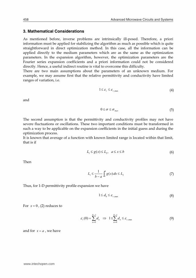
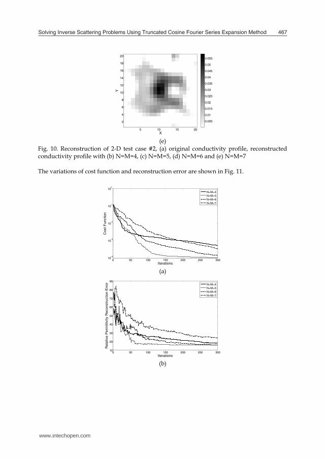
Fig. 10. Reconstruction of 2-D test case #2, (a) original conductivity profile, reconstructed conductivity profile with (b) N=M=4, (c) N=M=5, (d) N=M=6 and (e) N=M=7 The variations of cost function and reconstruction error are shown in Fig. 11.
(a)
(b)
X
Y
5 10 15 20
2
4
6
8
10
12
14
16
18
20
0.005
0.01
0.015
0.02
0.025
0.03
0.035
0.04
0.045
0.05
0.055
0 50 100 150 200 250 30010
-4
10-3
10-2
10-1
100
Iterations
Cos
t Fun
ctio
n
N=M=4N=M=5N=M=6N=M=7
0 50 100 150 200 250 30010
20
30
40
50
60
70
80
90
Iterations
Rel
ativ
e P
erm
ittiv
ity R
econ
stru
ctio
n E
rror
N=M=4N=M=5N=M=6N=M=7
www.intechopen.com
Solving Inverse Scattering Problems Using Truncated Cosine Fourier Series Expansion Method 467
(c) (d)
(e)
Fig. 9. Reconstruction of 2-D test case #2, (a) original permittivity profile, reconstructed permittivity profile with (b) N=M=4, (c) N=M=5, (d) N=M=6 and (e) N=M=7
(a) (b)
(c) (d)
X
Y
5 10 15 20
2
4
6
8
10
12
14
16
18
20
1
1.2
1.4
1.6
1.8
2
2.2
2.4
X
Y
5 10 15 20
2
4
6
8
10
12
14
16
18
20
1
1.5
2
2.5
X
Y
5 10 15 20
2
4
6
8
10
12
14
16
18
20
1
1.5
2
2.5
3
X
Y
5 10 15 20
2
4
6
8
10
12
14
16
18
20
0
0.005
0.01
0.015
0.02
0.025
0.03
0.035
0.04
X
Y
5 10 15 20
2
4
6
8
10
12
14
16
18
20
0
0.005
0.01
0.015
0.02
0.025
0.03
0.035
0.04
X
Y
5 10 15 20
2
4
6
8
10
12
14
16
18
20
0.005
0.01
0.015
0.02
0.025
0.03
0.035
X
Y
5 10 15 20
2
4
6
8
10
12
14
16
18
20
0.005
0.01
0.015
0.02
0.025
0.03
0.035
(e)
Fig. 10. Reconstruction of 2-D test case #2, (a) original conductivity profile, reconstructed conductivity profile with (b) N=M=4, (c) N=M=5, (d) N=M=6 and (e) N=M=7 The variations of cost function and reconstruction error are shown in Fig. 11.
(a)
(b)
X
Y
5 10 15 20
2
4
6
8
10
12
14
16
18
20
0.005
0.01
0.015
0.02
0.025
0.03
0.035
0.04
0.045
0.05
0.055
0 50 100 150 200 250 30010
-4
10-3
10-2
10-1
100
Iterations
Cos
t Fun
ctio
n
N=M=4N=M=5N=M=6N=M=7
0 50 100 150 200 250 30010
20
30
40
50
60
70
80
90
Iterations
Rel
ativ
e P
erm
ittiv
ity R
econ
stru
ctio
n E
rror
N=M=4N=M=5N=M=6N=M=7
www.intechopen.com
Advanced Microwave Circuits and Systems468
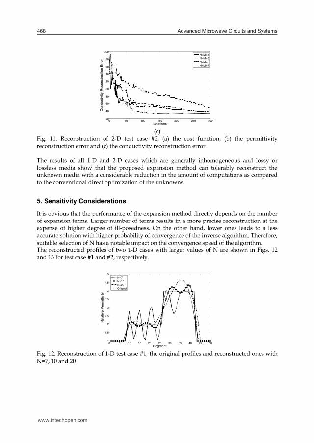
(c)
Fig. 11. Reconstruction of 2-D test case #2, (a) the cost function, (b) the permittivity reconstruction error and (c) the conductivity reconstruction error The results of all 1-D and 2-D cases which are generally inhomogeneous and lossy or lossless media show that the proposed expansion method can tolerably reconstruct the unknown media with a considerable reduction in the amount of computations as compared to the conventional direct optimization of the unknowns.
5. Sensitivity Considerations
It is obvious that the performance of the expansion method directly depends on the number of expansion terms. Larger number of terms results in a more precise reconstruction at the expense of higher degree of ill-posedness. On the other hand, lower ones leads to a less accurate solution with higher probability of convergence of the inverse algorithm. Therefore, suitable selection of N has a notable impact on the convergence speed of the algorithm. The reconstructed profiles of two 1-D cases with larger values of N are shown in Figs. 12 and 13 for test case #1 and #2, respectively.
Fig. 12. Reconstruction of 1-D test case #1, the original profiles and reconstructed ones with N=7, 10 and 20
0 50 100 150 200 250 30020
40
60
80
100
120
140
160
180
200
Iterations
Con
duct
ivity
Rec
onst
ruct
ion
Err
or
N=M=4N=M=5N=M=6N=M=7
0 5 10 15 20 25 30 35 40 45 501
1.5
2
2.5
3
3.5
4
4.5
5
Segment
Rel
ativ
e P
erm
ittiv
ity
N=7N=10N=20Original
(a)
(b)
Fig. 13. Reconstruction of 1-D test case #2, the original profiles and reconstructed ones with N=7, 15 and 25, (a) permittivity profile and (b) conductivity profile It is seen that increasing the number of expansion terms results oscillatory reconstruction because of the more ill-posedness of the problem. We can come to similar conclusion for 2-D cases by comparing different parts of Figs. 7, 9 and 10. Our experiences in studying various permittivity and conductivity profiles reconstruction show that choosing the number of expansion terms between 5 and 10 may be suitable for most of the reconstruction problems.
6. Conclusion
A computationally efficient method which is based on combination of the cosine Fourier series expansion, an EM solver and a global optimizer has been proposed for solving 1-D and 2-D inverse scattering problems. The mathematical formulations of the method have been derived completely and the algorithm has been examined for reconstruction of several inhomogeneous lossless and lossy cases. With a considerable reduction in the number of the unknowns and consequently the required number of populations and optimization iterations, along with no need to the regularization term, the relative permittivity and conductivity profiles have been reconstructed successfully. It has been shown by sensitivity
0 5 10 15 20 25 30 35 40 45 501
1.5
2
2.5
3
3.5
4
Segment
Rel
ativ
e P
erm
ittiv
ity
OriginalN=7N=15N=25
0 5 10 15 20 25 30 35 40 45 500
0.005
0.01
0.015
0.02
0.025
0.03
0.035
0.04
0.045
0.05
Segmant
Con
duct
ivity
OriginalN=7N=15N=25
www.intechopen.com

Solving Inverse Scattering Problems Using Truncated Cosine Fourier Series Expansion Method 469
(c)
Fig. 11. Reconstruction of 2-D test case #2, (a) the cost function, (b) the permittivity reconstruction error and (c) the conductivity reconstruction error The results of all 1-D and 2-D cases which are generally inhomogeneous and lossy or lossless media show that the proposed expansion method can tolerably reconstruct the unknown media with a considerable reduction in the amount of computations as compared to the conventional direct optimization of the unknowns.
5. Sensitivity Considerations
It is obvious that the performance of the expansion method directly depends on the number of expansion terms. Larger number of terms results in a more precise reconstruction at the expense of higher degree of ill-posedness. On the other hand, lower ones leads to a less accurate solution with higher probability of convergence of the inverse algorithm. Therefore, suitable selection of N has a notable impact on the convergence speed of the algorithm. The reconstructed profiles of two 1-D cases with larger values of N are shown in Figs. 12 and 13 for test case #1 and #2, respectively.
Fig. 12. Reconstruction of 1-D test case #1, the original profiles and reconstructed ones with N=7, 10 and 20
0 50 100 150 200 250 30020
40
60
80
100
120
140
160
180
200
Iterations
Con
duct
ivity
Rec
onst
ruct
ion
Err
or
N=M=4N=M=5N=M=6N=M=7
0 5 10 15 20 25 30 35 40 45 501
1.5
2
2.5
3
3.5
4
4.5
5
Segment
Rel
ativ
e P
erm
ittiv
ity
N=7N=10N=20Original
(a)
(b)
Fig. 13. Reconstruction of 1-D test case #2, the original profiles and reconstructed ones with N=7, 15 and 25, (a) permittivity profile and (b) conductivity profile It is seen that increasing the number of expansion terms results oscillatory reconstruction because of the more ill-posedness of the problem. We can come to similar conclusion for 2-D cases by comparing different parts of Figs. 7, 9 and 10. Our experiences in studying various permittivity and conductivity profiles reconstruction show that choosing the number of expansion terms between 5 and 10 may be suitable for most of the reconstruction problems.
6. Conclusion
A computationally efficient method which is based on combination of the cosine Fourier series expansion, an EM solver and a global optimizer has been proposed for solving 1-D and 2-D inverse scattering problems. The mathematical formulations of the method have been derived completely and the algorithm has been examined for reconstruction of several inhomogeneous lossless and lossy cases. With a considerable reduction in the number of the unknowns and consequently the required number of populations and optimization iterations, along with no need to the regularization term, the relative permittivity and conductivity profiles have been reconstructed successfully. It has been shown by sensitivity
0 5 10 15 20 25 30 35 40 45 501
1.5
2
2.5
3
3.5
4
Segment
Rel
ativ
e P
erm
ittiv
ity
OriginalN=7N=15N=25
0 5 10 15 20 25 30 35 40 45 500
0.005
0.01
0.015
0.02
0.025
0.03
0.035
0.04
0.045
0.05
Segmant
Con
duct
ivity
OriginalN=7N=15N=25
www.intechopen.com

Advanced Microwave Circuits and Systems470
analysis that for obtaining well-posedness as well as accurate reconstruction simultaneously, the number of expansion terms must be chosen intelligently.
7. References
Cakoni, F. & Colton, D. (2004). Open problems in the qualitative approach to inverse electromagnetic scattering theory. Euro. Jnl. of Applied Mathematics, Vol. 00, (1–15)
Caorsi, S.; Ciaramella, S.; Gragnani, G. L. & Pastorino, M. (1995). On the use of regularization techniques in numerical invere-scattering solutions for microwave imaging applications. IEEE Trans. Microwave Theory Tech., Vol. 43, No. 3, (March). (632–640)
Colton, D. & Paivarinta, L. (1992). The uniqueness of a solution to an inverse scattering problem for electromagnetic waves. Arc. Ration. Mech. Anal., Vol. 119, (59–70)
Isakov, V. (1993). Uniqueness and stability in multidimensional inverse problems,” Inverse Problems, Vol. 9, (579–621)
Rekanos, I. T. (2008). Shape reconstruction of a perfectly conducting scatterer using differential evolution and particle swarm optimization. IEEE Trans. Geosci. Remote Sens., Vol. 46, No. 7, (July). (1967-1974)
Robinson, J. & Rahmat-Samii, Y. (2004). Particle swarm optimization in electromagnetics. IEEE Transactions on Antennas and Propagation, Vol. 52, No. 2, (397-407)
Semnani, A. & Kamyab, M. (2008). Truncated cosine Fourier series expansion method for solving 2-D inverse scattering problems. Progress In Electromagnetics Research, Vol. 81, (73-97)
Semnani, A. & Kamyab, M. (2009). An enhanced hybrid method for solving inverse scattering problems. IEEE Transaction on Magnetics, Vol. 45, No. 3, (March). (1534-1537)
Storn, R. & Price, K. (1997). Differential evolution – A simple and efficient heuristic for global optimization over continuous space. J. Global Optimization, Vol. 11, No. 4, (Dec). (341–359)
Taflove, A. & Hagness, S. C. (2005). Computational Electrodynamics: The finite-difference time-domain method, Third Edition, Artech House
Tikhonov, A. N. & Arsenin, V. Y. (1977). Solutions of Ill-Posed Problems, Winston, Washington, DC
www.intechopen.com

Advanced Microwave Circuits and SystemsEdited by Vitaliy Zhurbenko
ISBN 978-953-307-087-2Hard cover, 490 pagesPublisher InTechPublished online 01, April, 2010Published in print edition April, 2010
InTech EuropeUniversity Campus STeP Ri Slavka Krautzeka 83/A 51000 Rijeka, Croatia Phone: +385 (51) 770 447 Fax: +385 (51) 686 166www.intechopen.com
InTech ChinaUnit 405, Office Block, Hotel Equatorial Shanghai No.65, Yan An Road (West), Shanghai, 200040, China
Phone: +86-21-62489820 Fax: +86-21-62489821
This book is based on recent research work conducted by the authors dealing with the design anddevelopment of active and passive microwave components, integrated circuits and systems. It is divided intoseven parts. In the first part comprising the first two chapters, alternative concepts and equations for multiportnetwork analysis and characterization are provided. A thru-only de-embedding technique for accurate on-wafer characterization is introduced. The second part of the book corresponds to the analysis and design ofultra-wideband low- noise amplifiers (LNA).
How to referenceIn order to correctly reference this scholarly work, feel free to copy and paste the following:
Abbas Semnani and Manoochehr Kamyab (2010). Solving Inverse Scattering Problems Using TruncatedCosine Fourier Series Expansion Method, Advanced Microwave Circuits and Systems, Vitaliy Zhurbenko (Ed.),ISBN: 978-953-307-087-2, InTech, Available from: http://www.intechopen.com/books/advanced-microwave-circuits-and-systems/solving-inverse-scattering-problems-using-truncated-cosine-fourier-series-expansion-method

© 2010 The Author(s). Licensee IntechOpen. This chapter is distributedunder the terms of the Creative Commons Attribution-NonCommercial-ShareAlike-3.0 License, which permits use, distribution and reproduction fornon-commercial purposes, provided the original is properly cited andderivative works building on this content are distributed under the samelicense.