S O LV I N G L A R G E S C A L E E I G E N VA L U E P R O B L E M S I N A M O R P H O U SM AT E R I A L S

giuseppe accaputo

Computational Science and EngineeringETH Zürich

Master Thesis

supervisors:

Prof. Dr. Peter ArbenzDr. Peter Derlet

Giuseppe Accaputo: Solving Large Scale Eigenvalue Problems in Amorphous Materials,© September 2017

The journey of a thousand miles begins with a single step.

— Lao Tzu

Dedicated to my parents, Teresa and Paolo, and my sister, Alessia, for all theirlove, patience, kindness, and support throughout my studies at the ETH Zürich.

A B S T R A C T

Amorphous solids, like metallic glasses exhibit an excess of states in the low fre-quency regime very close to the Boson peak, and the precise nature of these lowfrequency vibrations remains unclear.

The purpose of this thesis is to investigate the use of a polynomial filtered eigen-solver for the computation and study of low frequency eigenmodes of a Hessianmatrix located in a specific interval close to the Boson peak regime.

A distributed-memory parallel implementation of a polynomial filtered eigen-solver is presented. Our implementation is then applied to Hessian matrices ofdifferent atomistic bulk metallic glass structures derived from molecular dynamicssimulations for the computation of low frequency eigenmodes close to the Bosonpeak region. In addition, we demonstrate the parallel scalability of our implemen-tation on multicore nodes.

Our resulting calculations successfully concur with previous results [5], andanomalous behavior of the particles in the region close to the Boson peak canbe observed from the data.

v

A C K N O W L E D G M E N T S

I want to thank Professor Arbenz and Peter Derlet for the possibility to work onthis project, for their knowledge, patience and for their time. Further, I want tothank Dmitry Ozerov for his extensive, speedy and kind help with setting every-thing up and running computations on the Ra cluster at PSI. Finally, I want tothank my girlfriend Mirjam for all her love, support, and patience throughout thisexciting period of time in my life.

vii

C O N T E N T S

1 introduction 1

2 background 3

2.1 Polynomial Filtering 3

2.1.1 Least-Squares Polynomial Filters 3

2.1.2 Choosing the Degree of the Filter 5

2.1.3 Balancing the Filter 5

2.2 The Thick-Restart Lanczos Algorithm 8

3 implementation 13

3.1 Trilinos 13

3.1.1 Epetra 14

3.1.2 Anasazi 14

3.1.3 Teuchos 14

3.2 Parallelization 14

3.3 Parallel Matrix Import 17

3.4 Estimation of the Extremal Eigenvalues of A 17

3.5 Estimation of the Eigenvalue Count in a Specified Interval 18

3.6 Computation of the Polynomial Filter ρk 20

3.7 Combining the Eigensolver and Polynomial Filtering 23

3.8 Computation of the Polynomial Filter Operator ρk(A) 24

4 experimental results 27

4.1 Eigenmode Computations 27

4.1.1 Experimental Setup 27

4.1.2 Participation Ratio and Displacement Visualization 27

4.2 Performance Measurements 31

4.2.1 Experimental Setup 31

4.2.2 Polynomial Filter Operator ρk(H) 31

5 conclusion and future developments 35

a appendix a 37

a.1 User Manual: BosonPeak Utility 37

a.1.1 Deploying the BosonPeak Utility on the Euler (ETH Zürich)and/or Ra (PSI) Cluster 37

a.1.2 Code Compilation 37

a.1.3 Configuring the BosonPeak Utility to Run Different Calcula-tions 38

a.1.4 Building and Running the BosonPeak Unit Tests 41

a.2 Using the Polynomial Filter MATLAB Implementation 41

a.3 Converting MM Files Storing Large Symmetric Matrices to TrilinosCompatible HDF5 Files 45

bibliography 47

ix

L I S T O F F I G U R E S

Figure 1 Polynomial filters ρk of degree k = 11 for the interval [−0.2, 0.2],using three different smoothing approaches. 5

Figure 2 Polynomial filters ρk (Eq. (5)) of different degrees k for theinterval [ξ, η] = [−0.1, 0.5], using three different thresholdsφ and Jackson smoothing. The dotted lines connect ρk(ξ)

to ρk(η) for each polynomial filter, clearly showing ρk(ξ) 6=ρk(η). 6

Figure 3 Polynomial filters ρk (Eq. (5)) of different degrees k for theinterval [ξ, η] = [−0.1, 0.5], using three different thresholdsφ and Jackson smoothing. Each polynomial filter has beenbalanced such that ρk(ξ) = ρk(η) = τ (dotted lines). 8

Figure 4 Polynomial filters ρk (Eq. (5)) of different degrees k for theinterval [ξ, η] = [0.75, 1], using three different thresholdsφ and Jackson smoothing. Each polynomial filter has beenbalanced such that ρk(ξ) = τ (dotted lines). 9

Figure 5 Row-wise distribution pattern of a matrix A ∈ R6×6 using 3

MPI ranks. 15

Figure 6 Handling end interval cases by using different degrees forthe polynomial filter ρk. 21

Figure 7 Eigenvalues λ ∈ [0.1, 2.0] of the different samples Hi, i =

1, 2, . . . , 8 plotted against the participation ratios. 29

Figure 8 Displacement plots for different eigenmodes of H1. The plotsshow a cut along the x − y plane (δz = 0.15 Å) containingthe particle with the largest displacement. The arrows areproportional to the displacements of the particles, and thedisplacements have been magnified ×300 for visibility rea-sons. 30

Figure 9 Measured speedup and parallel efficiency of the polynomialoperator implementation with k = 500 and b = 32, with thetime measurements being averaged over 10 runs. 32

Figure 10 Measured speedup and parallel efficiency of the matrix-multivector multiplication in Eq. (57) with k = 151 andb = 128, with the time measurements being averaged over10 runs. 33

Figure 11 Weak scaling measurements of the matrix-multivector mul-tiplication in Eq. (57) with increasing block size b (left) andincreasing polynomial degree k (right). 33

Figure 12 Strong scaling measurements of the matrix-multivector mul-tiplication in Eq. (57). The blue line results from a linearregression using the measured timings. 34

Figure 13 Polynomial filter ρk (Eq. (5)) computed and plotted by usingthe MATLAB code displayed in Listing 6. 45

x

L I S T O F TA B L E S

Table 1 Tabular overview of properties of the Hessian matrices H1, . . . , H8

of a system with N = 256000 atoms. The second columncontains the Number of Nonzeros (NNZ) of Hi, the thirdcolumn shows the total number of eigenvalues λj ∈ [0.1, 2],and in the third column the maximal residual norm over allcomputed residual norms ‖rj‖ for a given Hi is displayed,where the residual vector is defined as rj = Hiuj − λjuj.Finally, in the last column the Time to Solution (Time to So-lution (TTS)) for the eigensolver part of the utility (Line 7

in Algorithm 3) is shown; the TTS is based on computationswith 48 cores on Euler. 28

L I S T I N G S

Listing 1 Configuration of the extremal eigenvalues to be used for thetransformation of the matrix as defined in Eq. (6). 38

Listing 2 Extended configuration for the approximation of the extremaleigenvalues. 39

Listing 3 Configuration for the estimation of the eigenvalue count 39

Listing 4 Complete configuration for the computation of eigenpairsin a specific interval of the spectrum. 40

Listing 5 Example code showing the usage of the MATLAB imple-mentation of the polynomial filter for the computation ofeigenvalues in a specific interval of interest. We are using asimple diagonal matrix A with spectrum σ = {1, 2, 3, 4, . . . , 20}and compute all the eigenvalues λi in the interval [11.5, 14.2].Before running this code it is important to first load allthe necessary environment variables by running the setup

-<euler|psi>.sh script as described in Section A.1.1. 41

Listing 6 Example code showing the usage of the MATLAB imple-mentation of the polynomial filter for the visualization ofthe resulting filter. Fig. 13 shows the resulting plot from thiscode. Before running this code it is important to first load allthe necessary environment variables by running the setup-<

euler|psi>.sh script as described in Section A.1.1. 44

xi

xii acronyms

A C R O N Y M S

mpi Message Passing Interface

crs Compressed Row Storage

rcp Reference Counting Pointer

bksm a block version of the Krylov-Schur method

pfo Polynomial Filter Operator

hdf5 Hierarchical Data Format 5

mm MatrixMarket

spmmm sparse Matrix-Multivector Multiplication

i .i .d. identically independently distributed

tts Time to Solution

nnz Number of Nonzeros

dos Density of States

bpu BosonPeak Utility

1I N T R O D U C T I O N

In condensed matter physics, an amorphous or disordered solid is a solid thatlacks the long-range order in the position of the atoms characteristic of a crystal.

For a crystal, vibrational excitations are understood in terms of quantized planewaves, the phonons, and in the low frequency regime the vibrational modes are theacoustic phonons. In the case of disordered solids, such as metallic glasses, it hasbeen shown that the majority of the vibrations are not plane waves. Propagativemodes, including plane waves are restricted to the low frequency regime, andlocalized modes occupy the high frequency tail of the spectrum.

For various amorphous solids, an excess of low frequency vibrations as com-pared to the Debye prediction has been observed. The origin of these modes inexcess is called the Boson peak, which historically has been measured via Ramanspectroscopy. At low frequencies and long wave-lengths, acoustic plane waves donot interact with disorder, and thus can still propagate in disordered solids. Oncethe frequency is increased beyond the Ioffe-Regel limit, the acoustic plane wavesinteract with the disorder and are significantly scattered. This strong scatteringregime occurs around the Boson peak position, and the exact origin of this phe-nomenon and its connection to the Boson peak is still debated.

Molecular dynamics simulations are able to produce metallic glasses. To decideon the nature of a mode, the Hessian matrix — a square matrix of second-orderpartial derivatives of the potential energy V — of such a generated system has tobe diagonalized. An analysis based on the computed eigenfrequencies and eigen-vectors would tell whether a mode is a propagating plane wave or not.

In our case, the matrix of interest is the Hessian matrix H of atomistic bulk metal-lic glass structures derived from molecular dynamics simulations using a binaryLennard Jones pair potential [5]. For a system consisting of N atoms, the vibra-tional modes of interest can be calculated by solving the real symmetric eigenvalueproblem defined by

Hui = λiui, H ∈ R3N×3N , ui ∈ R3N , i = 1, . . . , 3N , (1)

where λi = ω2i with ωi being the fundamental frequency and ui is the eigenmode

or eigenvector representing the displacement of the particles in the system. Further,the eigenvalues λi are arranged in ascending order, i.e. λmin = λ1 ≤ λ2 ≤ · · · ≤λ3N = λmax.

We are interested in obtaining the significant portion of the long-wavelength(low-frequency) vibrational eigenmodes close to the Boson peak, which will beanalyzed to investigate the relationship between the atomic-scale structure of themetallic glass and the Boson peak regime. This task requires the computation of alleigenvalues that are located in an interval close to the Boson peak region, includingthe associated eigenvectors.

Extreme eigenvalue problems, where the interval of interest [ξ, η] is located atthe end of the spectrum, i.e., when ξ = λmin or η = λmax are handled rather well by

1

2 introduction

most methods. The situation when [ξ, η] lies within the boundaries of the spectrumis harder to solve in general and is called an interior eigenvalue problem.

The interval of interest close to the Boson peak region is located in an interiorregion of the spectrum of the Hessian matrix H, and thus the problem stated in Eq.(1) is an interior eigenvalue problem.

For a general diagonalizable square matrix A of dimensions n × n, a frequentapproach to obtain part of the spectrum in an interior interval is to apply theLanczos algorithm to a transformed matrix B = ρ(A), where ρ is either a ratio-nal function or a polynomial. Nonetheless, the best known approach for interioreigenvalue problems is based on a shift-and-invert approach, where the Lanczosalgorithm is applied to B = (A− σI)−1. σ is called the shift and is selected to pointto the eigenvalues in the interval of interest. With the shift-and-invert transforma-tion, the eigenvalues of A closest to the shift σ are then mapped to the extremeones of B. Since we are working with an inverse matrix, shift-and-invert requires afactorization of the matrix A− σI which is not always readily available and can berather expensive to compute in some cases. Polynomial filtering instead replaces(A− σI)−1 by a polynomial ρ(A) such that all eigenvalues of A in [ξ, η] are trans-formed into dominant eigenvalues of ρ(A).

The goal of this thesis is to investigate the usage of the polynomial filters pre-sented in [12] combined with the thick-restart Lanczos algorithm to compute eigen-values and corresponding eigenvectors in an interior interval of the spectrum ofthe Hessian matrix H close to the Boson peak regime.

The thesis is organized as follows: Chapter 2 introduces the concept of polyno-mial filters and explains the idea behind the thick-restart Lanczos algorithm. Chap-ter 3 provides details about our implementation and the general parallelization ofour code. Next, in Chapter 4 results from interval-specific eigenpair computationswith Hessian matrices of large systems and various performance measurementsare discussed. Finally, the thesis ends with concluding remarks about our workand results in Chapter 5, and an outlook on possible enhancements of our imple-mentation based on the physical problem at hand is given.

2B A C K G R O U N D

In the first part of this chapter we present the concept of least-squares polynomialfilters as presented in [12], and how it can be applied to filter unwanted eigenval-ues outside of an interval of interest.

In the second part we introduce the thick-restart version of the Lanczos algo-rithm, which later in this thesis will be combined with the polynomial filter for thecomputation of interval-specific eigenpairs.

2.1 polynomial filtering

Polynomial filtering is a process by which a n × n real symmetric (or complexHermitian) matrix A is replaced by a function ρ(A), where the filter function ρ hasthe property of filtering out unwanted eigenvalues.

Suppose we want to compute eigenvalues in the interval of interest [ξ, η] ⊂ [a, b],where the interval [a, b] contains the complete spectrum of A. The polynomialρ(λ) is chosen in such a way that all eigenvalues of A in [ξ, η] are transformedinto dominant eigenvalues of ρ(A). Therefore, due to the nature of the Lanczosalgorithm the dominant eigenvalues of ρ(A) will be approximated first.

The polynomials ρ we are using in this work are least-squares approximationsto the Dirac-delta function using a series expansion based on Chebyshev polyno-mials of the first kind [12]. In the following sections we summarize the conceptspresented by Li et al in [12].

2.1.1 Least-Squares Polynomial Filters

The Dirac-delta distribution is a generalized function that was introduced by PaulDirac for the representation of an idealized point object, such as a point mass orpoint charge. It is a function that is equal to zero everywhere except for t = γ,where it represents a spike that is infinitely high and the integral over the line isequal to 1. In the approach presented in [12], the filter is a least-squares approxi-mation to the Dirac-delta function.

The approximate polynomial ρk(t) of the Dirac-delta δγ centered at γ is realizedby expanding δγ as a degree k Chebyshev polynomial series defined as

ρk(t) =k

∑j=0

µjTj(t) (2)

with

µj =

12 if j = 0

cos(j arccos(γ)) otherwise ,(3)

3

4 background

where k is the degree of the polynomial and the Chebyshev polynomial Tj of thefirst kind of order j is defined as

Tj(t) = cos(n arccos(t)), t ∈ [−1, 1], j = 0, 1, 2, . . . (4)

Since the Dirac-delta function is a distribution — and thus expanding it using Eq.(2) may not be mathematically rigorous or permissible — the authors state with[12, Proposition 3.1] that the polynomial defined as

ρk(t) = ρk(t)/ρk(γ) (5)

is the polynomial that minimizes ‖r(t)‖w over all polynomials r of degree ≤ k,such that r(γ) = 1, with ‖ · ‖w being the Chebyshev L2-norm.

If we want to apply the polynomial ρk in Eq. (5) to the matrix A using theChebyshev polynomials as defined in Eq. (4), we need to map the eigenvalues of Ato the reference interval [−1, 1], which can be accomplished by using the followinglinear map from [λmin, λmax] to [−1, 1]:

A =A− cI

dwith c =

λmax + λmin

2, d =

λmax − λmin

2. (6)

The extremal eigenvalues λmin and λmax of A used in Eq. (6) can be approx-imated by lower and upper bounds obtained by adequate perturbations of thelargest and smallest eigenvalue, which can be computed by running a small num-ber of iterations of the Lanczos algorithm.

2.1.1.1 Oscillations and Damping

The expansion of discontinuous functions will exhibit oscillations near the discon-tinuities, which are known as Gibbs oscillations. To alleviate this behavior it is thususual to add smoothing coefficients gk

j so that Eq. (2) is replaced by

ρk(t) =k

∑j=0

gkj µjTj(t) . (7)

These coefficients can be calculated by using different smoothing approaches.Jackson smoothing [9, 14] is one of the best known approaches, and computes thesmoothing factors gk

j by using the formula

gkj =

sin(j + 1)αk

(k + 2) sin αk+

(1− j + 1

k + 2

)cos(j αk) with αk =

π

k + 2. (8)

Another smoothing approach proposed by Lanczos [11, Chapter 4] is called σ-smoothing and uses simpler smoothing coefficients:

σk0 = 1, σk

j =sin(jθk)

jθk, j = 1, . . . , k, with θk =

π

k + 1. (9)

Fig. 1 shows three polynomial filters ρk of degree k = 11 for the interval [−0.2, 0.2],one of which is without smoothing and the other two with Jackson damping orthe Lanczos σ-damping, respectively.

2.1 polynomial filtering 5

-1 -0.5 0 0.5 1

-0.4

-0.2

0

0.2

0.4

0.6

0.8

1

No Smoothing

Lanczos Smoothing

Jackson Smoothing

Figure 1: Polynomial filters ρk of degree k = 11 for the interval [−0.2, 0.2], using threedifferent smoothing approaches.

2.1.2 Choosing the Degree of the Filter

The degree of the polynomial filter ρk is automatically computed based on thedefined interval of interest [ξ, η] ⊂ [λmin, λmax] and on the type of smoothingcoefficients to be used. The interval boundaries ξ and η are first transformed usingEq. (6) to ξ and η, respectively:

ξ = (ξ − c)/d , (10)

η = (η − c)/d . (11)

These transformations guarantee that ξ, η ∈ [−1, 1]. The procedure then starts witha low degree polynomial and increases k until the values of ρk(ξ) and ρk(η) bothfall below a certain threshold φ. Once this happens, we set τ = min{ρk(ξ), ρk(η)},with τ < φ being a bar value that will be used in Section 2.1.3 to filter out unwantedeigenvalues.

In Fig. 2 three scaled polynomial filters ρk with different thresholds φ for theinterval [ξ, η] = [−0.1, 0.5] are shown. The dotted lines in Fig. 2 connect the pointρk(ξ) to ρk(η). As we can recognize from the slope of the dotted line connectingthe two points, we have ρk(ξ) 6= ρk(η) which is not very helpful in selecting thedesired eigenvalues in the interval [ξ, η]. For this reason, in the next section abalancing step is introduced, such that ρk(ξ) = ρk(η) is guaranteed.

2.1.3 Balancing the Filter

For the selection of eigenvalues λ in the interval of interest [ξ, η] it is desirableto have a polynomial filter ρk whose values at the transformed boundaries ξ andη are the same. This is accomplished by moving the center γ of the Dirac-deltafunction δγ away from the midpoint of the interval [ξ, η]. Once we have adjusted

6 background

-1 -0.5 0 0.5 1

-0.2

0

0.2

0.4

0.6

0.8

1

1.2

Figure 2: Polynomial filters ρk (Eq. (5)) of different degrees k for the interval [ξ, η] =[−0.1, 0.5], using three different thresholds φ and Jackson smoothing. The dot-ted lines connect ρk(ξ) to ρk(η) for each polynomial filter, clearly showingρk(ξ) 6= ρk(η).

the center, and thus ρk(ξ) = ρk(η), determining if a computed eigenvalue θj ofρk(A) corresponds to an eigenvalue λj in [ξ, η] becomes a simple task, namely: Ifτ ≡ ρk(ξ) = ρk(η), then

λj ∈ [ξ, η] ⇐⇒ θj ≥ τ . (12)

Hence, finding all eigenvalues λj ∈ [ξ, η] can be accomplished by finding all eigen-values θj of ρk(A) that are greater than or equal to τ. It is important to mentionthat this step is only used as a preselection tool. The matrix A and ρk(A) share thesame eigenvectors u1, u2, . . . , un [7]. Thus, once all eigenpairs (θj, uj) with θj ≥ τ

have been computed, we can use the corresponding eigenvectors uj to extract theeigenvalues of A in [ξ, η] by first evaluating the Rayleigh quotient

λj = uTj Auj , (13)

and then check if λj ∈ [ξ, η].To adjust the center γ such that ρk(ξ) = ρk(η), the polynomial ρk from Eq. (7) is

first written in terms of the variable θt = arccos(t), i.e.

ρk(cos(θt)) =k

∑j=0

gkj cos(jθγ) cos(jθt) . (14)

Newton’s method is then used to solve the equation

ρk(cos(θξ))− ρk(cos(θη)) = 0 (15)

with respect to θγ. Since cos(jθγ) = µj in Eq. (14), with µj being defined in Eq. (3),it is important to note that the first smoothing coefficient gk

0 is multiplied by 1/2

2.1 polynomial filtering 7

to simplify notation, meaning that the first term with j = 0 is not 1 but rather 1/2.Using this notation and Eq. (14), Eq. (15) can be rewritten as

f (θγ) ≡ ρk(cos(θξ))− ρk(cos(θη))

=k

∑j=0

gkj cos(jθγ))[cos(jθξ)− cos(jθη))] = 0 . (16)

Next, Newton’s method requires the first derivative of f with respect to θγ,which is given by

f ′(θγ) = −k

∑j=0

gkj j sin(jθγ)[cos(jθξ)− cos(jθη)] . (17)

Further, the authors of [12] provide a good initial guess with a mid-angle definedas

θc =12(θξ + θη) , (18)

which often yields convergence of the Newton iteration in one or two steps. Still,in some cases (e.g. for low degree polynomials) Newton’s method may fail toconverge in two steps, and in these cases the roots of Eq. (16) are computed exactlyby solving the eigenvalue problem given by

12

Ct = γt , (19)

where

C =

0 2

1 0 1

1 0 1. . . . . . . . .

1 0 1

−β0 −β1 . . . . . . 1− βk−2 −βk−1

(20)

is a Hessenberg matrix in Rk×k, β j is defined as

β j =gk

j [cos(jθξ − cos(jθη))]

gkk[cos(kθξ − cos(kθη))]

, (21)

and t has components tj = cos(jθγ) = Tj(γ) (see [12, Appendix A] for a detailedderivation). The new center γnew is then taken to be the eigenvalue of C/2 that isclosest to the value cos(θc).

Fig. 3 shows three balanced polynomial filters ρk for the interval [ξ, η] = [−0.1, 0.5].In Fig. 2 the same interval has been used to compute the polynomials ρk withoutthe balancing step. By comparing the dotted lines in Fig. 3 to the ones in Fig. 2, wecan see that for all balanced polynomial filters shown in Fig. 3 ρk(ξ) = ρk(η) = τ

holds. Further, by comparing the value of each γ in both Figs. 2 and 3, respectively,we can see that in Fig. 3 the new midpoint γ of each approximated Dirac-delta

8 background

function has been moved away from the previous midpoint, thus yielding balancedpolynomials.

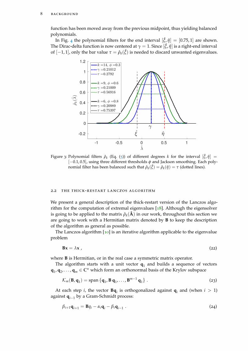
In Fig. 4 the polynomial filters for the end interval [ξ, η] = [0.75, 1] are shown.The Dirac-delta function is now centered at γ = 1. Since [ξ, η] is a right-end intervalof [−1, 1], only the bar value τ = ρk(ξ) is needed to discard unwanted eigenvalues.

-1 -0.5 0 0.5 1

-0.2

0

0.2

0.4

0.6

0.8

1

1.2

Figure 3: Polynomial filters ρk (Eq. (5)) of different degrees k for the interval [ξ, η] =[−0.1, 0.5], using three different thresholds φ and Jackson smoothing. Each poly-nomial filter has been balanced such that ρk(ξ) = ρk(η) = τ (dotted lines).

2.2 the thick-restart lanczos algorithm

We present a general description of the thick-restart version of the Lanczos algo-rithm for the computation of extremal eigenvalues [18]. Although the eigensolveris going to be applied to the matrix ρk(A) in our work, throughout this section weare going to work with a Hermitian matrix denoted by B to keep the descriptionof the algorithm as general as possible.

The Lanczos algorithm [10] is an iterative algorithm applicable to the eigenvalueproblem

Bx = λx , (22)

where B is Hermitian, or in the real case a symmetric matrix operator.The algorithm starts with a unit vector q1 and builds a sequence of vectors

q1, q2, . . . , qm ∈ Cn which form an orthonormal basis of the Krylov subspace

Km(B, q1) = span {q1, B q1, . . . , Bm−1 q1} . (23)

At each step i, the vector Bqi is orthogonalized against qi and (when i > 1)against qi−1 by a Gram-Schmidt process:

βi+1qi+1 = Bqi − αiqi − βiqi−1 . (24)

2.2 the thick-restart lanczos algorithm 9

-1 -0.5 0 0.5 1

-0.2

0

0.2

0.4

0.6

0.8

1

1.2

Figure 4: Polynomial filters ρk (Eq. (5)) of different degrees k for the interval [ξ, η] =[0.75, 1], using three different thresholds φ and Jackson smoothing. Each poly-nomial filter has been balanced such that ρk(ξ) = τ (dotted lines).

In theory, i.e. with exact arithmetic, this three-term recurrence computes an or-thonormal basis {q1, . . . , qm} of Km(B, q), but in the presence of rounding, orthog-onality between the qi’s is lost soon after at least one eigenvector starts converging.A remedy to this problem is to reorthogonalize the vectors when needed, suchthat the orthogonality among the qi’s to working precision is enforced. The m-stepLanczos algorithm is shown in Algorithm 1, in which Qj ≡ [q1, . . . , qj] containsthe basis constructed up to step j as its column vectors and a reorthogonalizationstep is included on Line 7 in Algorithm 1.

In the new orthonormal basis Qm the operator B is represented by the real sym-metric tridiagonal matrix

Tm =

α1 β1

β1 α2. . .

. . . . . . βm−1

βm−1 αm

, (25)

where the scalars αi, βi are those produced by the Lanczos algorithm. Eq. (24) canbe rewritten in the form

BQm = QmTm + βm+1qm+1eHm , (26)

where em is the mth column of the canonical basis and qm+1 is the last vectorcomputed by the Lanczos algorithm at step m.

Let (θ(m)i , y(m)

i ) be the eigenpair of Tm at the mth step of the process. The eigen-

values θ(m)i are called Ritz values and will approximate some of the eigenvalues

of B as m increases. The vectors u(m)i = Qmy(m)

i , known as Ritz vectors, will ap-

10 background

Algorithm 1 The m-step Lanczos algorithm

1: Input: A Hermitian matrix B ∈ Cn×n, and an initial unit vector q1 ∈ Cn.

2: q0 = 0, β1 = 0

3: for i = 1, 2, . . . , m do

4: w = Bqi − βiqi−1

5: αi = qHi w

6: w = w− αiqi

7: Reorthogonalize: w = w−Qi(QHi w)

8: βi+1 = ‖w‖2

9: if βi+1 = 0 then

10: qi+1 = a random vector of unit norm that is orthogonal to q1, . . . , qi

11: else

12: qi+1 = w/βi+1

proximate the related eigenvectors of B. The Ritz pair (θ(m)i , u(m)

i ) will be a goodapproximation to an eigenpair of B if the residual norm

‖r‖ = ‖Bui − θiui‖ (27)

is less than a prescribed threshold. Further, the Lanczos algorithm yields goodapproximations to extreme eigenvalues of B rather fast, whereas convergence toeigenvalues located deep inside the spectrum is much slower.

A disadvantage of the Lanczos algorithm is the fact that there is no way todetermine in advance how many steps will be needed. In many cases, convergenceto the eigenvalues of interest within a specified accuracy will not occur until thenumber of iterations m gets very large. Maintaining the orthogonality of such largebases becomes expensive and even intractable for large m.

To help maintain orthogonality and thus minimize the costs caused by reorthog-onalizing the bases, the dimension of the search space is limited and restartingschemes are introduced. Restarting means that the starting vector q1 is replacedwith an improved vector q∗1 (a Ritz vector computed during the previous itera-tions) and a new Lanczos decomposition with the new vector is computed. In thecase of a thick restart, the algorithm is restarted not with one but with multipleRitz vectors.

In the following we recall the steps from [12] for extending the standard Lanczosmethod shown in Algorithm 1 to the thick-restart Lanczos method as defined byWu and Simon [18].

Suppose that after m steps of the Lanczos algorithm we have l Ritz vectorsu1, u2, . . . , ul . We wish to use these Ritz vectors along with the last vector qm+1as restarting vectors. From [15, Proposition 6.8] we know that each Ritz vector uihas a residual in the direction of qm+1, i.e.

(B− θiI)ui = (βm+1eHm yi)qm+1 ≡ siqm+1 for i = 1, . . . , l . (28)

2.2 the thick-restart lanczos algorithm 11

By defining qi = ui and ql+1 = qm+1 and rewriting Eq. (28) in matrix form, itfollows that

BQl = QlΘl + ql+1sH , (29)

where Ql = [q1, . . . , ql], Θl = diag(θ1, . . . , θl), and sT = [s1, . . . , sl ].To compute the (l + 2)th basis vector ql+2, we compute Bql+1 and orthonormal-

ize it against the previous l + 1 basis vectors:

βl+2ql+2 = Bql+1 −l

∑i=1

siqi − αl+1ql+1 , (30)

where αl+1 = ql+1HBql+1.

After completing the first step after the restart, the following equation holds:

BQl+1 = Ql+1Tl+1 + βl+2ql+2eHl+1 with Tl+1 =

(Θl s

sH αl+1

). (31)

The algorithm now proceeds just like the Lanczos algorithm, i.e., qk for k ≥ l + 3is computed until the dimension reaches m. Selecting which Ritz pairs (θj, uj =

Qmyj) the algorithm should keep for the restart can be based on different heuristicschemes; we refer to [18, 19] for a few examples and further details.

The thick-restart Lanczos algorithm is sketched in Algorithm 2. A detailed de-scription of the thick-restart Lanczos method can be found in Wu and Simon [18].

12 background

Algorithm 2 Thick-restart Lanczos algorithm

1: Input: A Hermitian matrix B ∈ Cn×n and an initial unit vector q1 ∈ Cn.

2: q0 = 0, β1 = 0, Its = 0, lock = 0, U = [ ]

3: while Its ≤ MaxIts do

4: if l > 0 then

5: Perform thick restart step (30), which results in Ql+2 and Tl+1 in (31)

6: for i = l + 1, . . . , m do

7: w = Bqi − βiqi−1

8: αi = qHi w

9: w = w− αiqi

10: Reorthogonalize: w = w−Qi(QHi w)

11: βi+1 = ‖w‖2

12: if βi+1 = 0 then

13: qi+1 = a random vector of unit norm that is orthogonal to q1, . . . , qi

14: else

15: qi+1 = w/βi+1

16: Set Its = Its + 1

17: Results: Qm ∈ Cn×m and Tm ∈ Rm×m.

18: Compute all eigenpairs (θj, yj) of Tm and the norm of the correspondingresiduals defined in Eq. (28)

19: if the norm of all residuals is smaller than a prescribed threshold then

20: return the Ritz pairs (θj, uj = Qmyj) of interest (smallest or largest magni-tude of θj)

21: else

22: Select which vectors of the current basis should be used at the next restartbased on a heuristic scheme, e.g. [18, 19]

3I M P L E M E N TAT I O N

In this chapter we combine the methods from Chapter 2 and a few other usefultools into a utility that can be used to compute the eigenpairs of a n × n realsymmetric (or complex Hermitian) matrix A within a specified interval of interest[ξ, η] in parallel by simply providing an XML configuration file (see A.1). Theoutline of the utility can be found in Algorithm 3.

In Section 3.1 we first introduce Trilinos, the workhorse behind the numericalwork done by the utility. Next, in Section 3.2 we give some details about the distri-bution pattern used throughout our implementation for the distributed-memoryparallel computations. Finally, in the remaining sections we explain the ideas andimplementation details behind most of the steps in Algorithm 3.

Algorithm 3 The BosonPeak Utility

1. Import user-specified configuration via XML file (see A.1).

2. Import the matrix A.

3. If requested, estimate the extremal eigenvalues λmin, λmax of A using a smallnumber of Lanczos steps.

4. Transform the matrix A to A based on Eq. (6).

5. If requested, estimate the number of eigenvalues in the specified interval [ξ, η].

6. Compute the polynomial filter ρk using Algorithm 4.

7. Compute the eigenpairs (λj, uj) of the matrix A with λj ∈ [ξ, η] and residualnorms rj = ‖Auj − λjuj‖ using Algorithm 6

8. If requested, write the eigenvalues λj, eigenvectors uj and residual norms rj inthe MatrixMarket (MM) format to the hard disk.

3.1 trilinos

The utility is written in C++11 and uses Trilinos1 extensively, a collection of open-source software libraries, called packages, for the development of scientific applica-tions.

1 https://trilinos.org/

13

14 implementation

3.1.1 Epetra

The Epetra2 package provides classes for the construction and use of serial and dis-tributed parallel linear algebra objects, and many of the Trilinos solver packageswork with Epetra objects. The most used linear algebra objects in our implementa-tion are sparse, Compressed Row Storage (CRS) matrices, and collections of densevectors called multivectors. An Epetra_CrsMatrix object stores a sparse matrix inthe CRS format with real-valued double-precision entries. An Epetra_MultiVector

object instead stores each vector in a multivector as a contiguous array of double-precision numbers. Both objects are extensively used for sparse matrix-vector mul-tiplications in the various Trilinos solver packages.

3.1.2 Anasazi

Anasazi3 is a package that offers a collection of algorithms for solving large-scaleeigenvalue problems. As part of the package it provides solver managers to imple-ment a strategy for solving an eigenvalue problem.

3.1.3 Teuchos

The Teuchos package is a collection of common tools used throughout Trilinos.Among other things, it provides templated access to BLAS and LAPACK inter-faces, parameter lists that allow to specify parameters for different packages, andmemory management tools for aiding in correct allocation and deletion of mem-ory.

Part of the memory management tools is an implementation of a ReferenceCounting Pointer (RCP) class, which for an object tracks a count of the numberof references to it held by other objects. Once the counter reaches zero, the objectcan be destroyed. The advantage of a RCP is that the possibility of memory leaksin a program can be reduced, which is especially important when working withrather large objects, e.g. an Epetra_CrsMatrix object storing over 109 nonzero entries.RCP objects are heavily used throughout our implementation to manage large ob-jects, especially large temporary objects that are only needed during a fraction ofthe whole computation.

3.2 parallelization

Trilinos supports distributed-memory parallel computations through the MessagePassing Interface (MPI). Both the Epetra_CrsMatrix and the Epetra_Multivector ob-jects can be used in a distributed memory environment by defining data distribu-tion patterns using Epetra_Map objects.

The entries of a distributed object (such as rows or columns of a Epetra_CrsMatrix

or the rows of a Epetra_Multivector) are represented by global indices uniquely overthe entire object. A map essentially assigns global indices to available MPI ranks(further referred to as only ranks), which in our case a single rank corresponds —

2 https://trilinos.org/packages/epetra/

3 https://trilinos.org/packages/anasazi/

3.2 parallelization 15

but in general is not limited — to a single core on a processor. For example, if themap assigns the global row index i of a sparse matrix to a rank p, we say that therank p owns the global row index i. Within a rank, we refer to a global index usinga local index. In the specific example of a global row index i, this means that a rankp can access the local data of the global row i it owns by using the local index l(i),where the function l maps the global index i to a local index for the specific rank.

For the addressing, local and global indices in Epetra use by default a 32-bit inttype. Since our implementation is based on the C++11 language standard and wewant to allow computations with large matrices, we explicitely use 64-bit globalindices of type long long when working with distributed linear algebra objects.

An Epetra_Map object enapsulates the details of distributing data over MPI ranks.In our implementation, we use contiguous and one-to-one maps for the distributionof the rows of Epetra_CrsMatrix and Epetra_MultiVector objects. Contiguous meansthat the list of global indices on each MPI rank forms an interval and is strictlyincreasing. A one-to-one map instead allows a global index only to be owned bya single rank. For the columns, the distribution pattern we are using distributesthe complete set of global column indices for a given global row, meaning that ifa rank p owns the global row index i, it also owns all global column indices j onthat row, thus having local access to the global entry (i, j). The map used for thedistribution of the columns is thus not a one-to-one map, since a global columnindex can be owned by multiple ranks.

0

1

2

3

4

5

Figure 5: Row-wise distribution pattern of a matrix A ∈ R6×6 using 3 MPI ranks.

As an illustrative example we distribute the following 8 × 8 sparse matrix Aover 4 ranks using the previously specified distribution pattern for the rows andcolumns, respectively:

16 implementation

A =

1 2 0 0 5 0 0 7

0 0 0 4 0 2 3 1

10 0 11 0 0 100 0 0

0 0 0 120 13 0 0 0

0 0 0 0 0 1 3 4

77 0 18 0 0 0 0 6

10 20 55 0 0 0 0 0

0 0 0 0 11 153 131 0

(32)

The distribution of the matrix A over the 4 ranks looks as follows:

• Rank 0:

– Global row indices owned: {0, 1}– Global column indices owned: {0, 1, 3, 4, 5, 6, 7}– Global entries locally accessible:{(0, 0), (0, 1), (0, 4), (0, 7), (1, 3), (1, 5), (1, 6), (1, 7)}

• Rank 1:

– Global row indices owned: {2, 3}– Global column indices owned: {0, 2, 3, 4, 5}– Global entries locally accessible:{(2, 0), (2, 2), (2, 5), (3, 3), (3, 4)}

• Rank 2:

– Global row indices owned: {4, 5}– Global column indices owned: {0, 2, 5, 6, 7}– Global entries locally accessible:{(4, 5), (4, 6), (4, 7), (5, 0), (5, 2), (5, 7)}

• Rank 3:

– Global row indices owned: {6, 7}– Global column indices owned: {0, 1, 2, 4, 5, 6}– Global entries locally accessible:{(6, 0), (6, 1), (6, 2), (7, 4), (7, 5), (7, 6)}

Now that the data is distributed, each rank can start to work on the ownedglobal matrix entries. For this, the ranks need the local indices to the owned rowsand columns. This is accomplished by using a mapping function l(i) that maps aglobal index i to a local one. A specific rank can then use the local indices to locallyaccess the owned global entries. An example of such a mapping is shown for theglobal indices on rank 3:

• Rank 3:

3.3 parallel matrix import 17

– Local row indices: l(4) = 0, l(5) = 1

– Local column indices:l(0) = 0, l(2) = 1, l(5) = 2, l(6) = 3, l(7) = 4

Rank 3 can now use the local indices to access the data. For example, by locallysetting A(l(5), l(7)) = 49, the global entry A(5, 7) gets the value 49 set. Thesechanges to the structure of an Epetra_CrsMatrix object have to be committed viaa call to the FillComplete function, which for one helps construct communicationpatterns to support distributed sparse matrix-vector multiplications.

3.3 parallel matrix import

The matrix import implemented in the utility allows to efficiently import large ma-trices stored in a Hierarchical Data Format 5 (HDF5)4 file directly to a Epetra_CrsMatrix

object.HDF5 is a data model, library, and file format for storing and managing data

collections of all sizes and complexity. One of the advantages of using the HDF5

format to store and import large matrices is the possibility to use MPI to read theHDF5 files in parallel. For this reason Trilinos provides the EpetraExt::HDF5 classfor importing a matrix stored in a HDF5 file to a Epetra_CrsMatrix.

Since the EpetraExt::HDF5 class currently does not provide an import functionfor matrices with 64-bit global indices of type long long, we extended the classby a function suitable for working with 64-bit data. Further, because some of thematrices may be delivered in the MM format, in a preprocessing step a Pythonscript can be used to convert the matrices stored in the MM format to a HDF5 filesuitable for the import (see Appendix A.3).

3.4 estimation of the extremal eigenvalues of A

For the transformation of A to A, as shown in Eq. (6), we need to specify a value forthe extremal eigenvalues λmin and λmax of A. In case we want to approximate theextremal eigenvalues, we simply run a small number of Lanczos iterations (e.g. 10iterations in our case) for the approximation of the required extremal eigenvaluesdenoted by λmin and λmax, respectively.

In case the Lanczos method manages to return converged eigenvalues by onlyrunning a few iterations, we use λmin = λmin and λmax = λmax. In situationswhere the computation of the extremal eigenvalues does not converge, we simplysubtract (when approximating λmin) or add (when approximating λmax) a smallperturbation from the approximated eigenvalues by using

λmin = λmin − p · |λmin| , (33)

λmax = λmax + p · |λmax| , (34)

where p� 1 is a small perturbation factor.

4 https://support.hdfgroup.org/HDF5/

18 implementation

3.5 estimation of the eigenvalue count in a specified interval

The estimation of the number of eigenvalues located in a given interval is com-puted by approximating the trace of an eigenprojector [6]. This estimation willbe later needed (on Line 7 of Algorithm 3) to specify how many of the largesteigenvalues of ρk(A) the eigensolver specified in Algorithm 6 should compute andreturn. In the following we give a summary of the technique as presented by DiNapoli et al in [6].

Let λj, j = 1, . . . , n be the eigenvalues and u1, u2, . . . , un the associated orthonor-mal eigenvectors of our real, symmetric (or complex Hermitian) matrix A. For aspecified interval [ξ, η], with λmin ≤ ξ < η ≤ λmax, our aim is to count the numberof eigenvalues λi in the interval [ξ, η]. We estimate the eigenvalue count by seekingan approximation of the trace of the eigenprojector

P = ∑λi∈[ξ,η]

uiuTi . (35)

Since the eigenvalues of a projector are either zero or one, the trace of P in Eq.(35) is equal to the number of eigenvalues in [ξ, η]. Thus, the number of eigenvaluesµ[ξ,η] located in the interval [ξ, η] can be calculated by evaluating the trace of theprojector in Eq. (35):

µ[ξ,η] = tr(P) . (36)

Considering that the projector P is typically not available, we approximate it inthe form of a polynomial function of A. For this, we can interpret P as a character-istic function of the interval [ξ, η]:

P = h(A) where h(t) =

1 if t ∈ [ξ, η] ,

0 otherwise(37)

In our case, we approximate h(t) with a finite sum ψ(t) of Chebyshev polyno-mials, namely P ≈ ψ(A). Further, we estimate the trace of P using Hutchinson’sunbiased estimator [8]. Hutchinson showed that given a general matrix A and arandomly generated vector v with identically independently distributed (i.i.d.) ran-dom variables as entries, the equation E(vTAv) = tr(A) holds. Thus, the ideabehind the estimator is to compute an estimate Tnv of the trace tr(A) by generatingnv samples of random vectors vk, k = 1, . . . , nv and then computing the average ofvT

k Av over these samples:

tr(A) ≈ Tnv =1nv

nv

∑k=1

vTk Av . (38)

Hutchinson originally used i.i.d. Rademacher random variables, whereby eachentry of v assumes the values −1 or 1 with probability 1/2. In general, any se-quence of random vectors vk whose entries are i.i.d. random variables can be used,as long as the mean of their entries is zero [2]. In our case, we used a Gaussianestimator to compute Tnv in Eq. (38) by using normally distributed variables forthe entries of the random vectors vk. Despite the fact that the Gaussian estimator

3.5 estimation of the eigenvalue count in a specified interval 19

has a larger variance than that of Hutchinson, it shows better convergence in termsof the number of sample vectors nv [1].

The trace of P can now be computed as

µ[ξ,η] = tr(P) ≈ nnv

nv

∑k=1

vTk ψ(A)vk , (39)

where the sample vectors vk ∈ Rn are normalized to one ‖vk‖ = 1 and the factorn is introduced by this constraint.

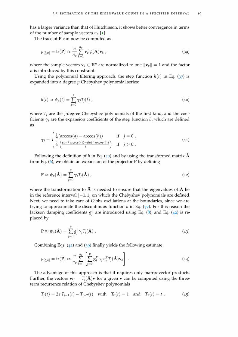
Using the polynomial filtering approach, the step function h(t) in Eq. (37) isexpanded into a degree p Chebyshev polynomial series:

h(t) ≈ ψp(t) =p

∑j=0

γjTj(t) , (40)

where Tj are the j-degree Chebyshev polynomials of the first kind, and the coef-ficients γj are the expansion coefficients of the step function h, which are definedas

γj =

1π (arccos(a)− arccos(b)) if j = 0 ,2π

(sin(j arccos(a))−sin(j arccos(b))

j

)if j > 0 .

(41)

Following the definition of h in Eq. (40) and by using the transformed matrix Afrom Eq. (6), we obtain an expansion of the projector P by defining

P ≈ ψp(A) =p

∑j=0

γjTj(A) , (42)

where the transformation to A is needed to ensure that the eigenvalues of A liein the reference interval [−1, 1] on which the Chebyshev polynomials are defined.Next, we need to take care of Gibbs oscillations at the boundaries, since we aretrying to approximate the discontinuos function h in Eq. (37). For this reason theJackson damping coefficients gp

j are introduced using Eq. (8), and Eq. (42) is re-placed by

P ≈ ψp(A) =p

∑j=0

gpj γjTj(A) . (43)

Combining Eqs. (42) and (39) finally yields the following estimate

µ[ξ,η] = tr(P) ≈ nnv

nv

∑k=1

[p

∑j=0

gpj γj vT

k Tj(A)vk

]. (44)

The advantage of this approach is that it requires only matrix-vector products.Further, the vectors wj = Tj(A)v for a given v can be computed using the three-term recurrence relation of Chebyshev polynomials

Tj(t) = 2 t Tj−1(t)− Tj−2(t) with T0(t) = 1 and T1(t) = t , (45)

20 implementation

which results in

wj = 2 A wj−1 −wj−2 with w0 = T0(A) v = v and w1 = T1(A) v = Av .(46)

In our implementation, by default we use nv = 40 and a polynomial degreep = 100 for the estimation of the eigenvalue count µ[ξ,η] with Eq. (44).

3.6 computation of the polynomial filter ρk

Algorithm 4 contains the needed elements for the computation of the polynomialfilter ρk as defined by Eqs. (5) and (7). The algorithm incorporates the ideas pre-sented in Section 2.1 and is mostly based (with some minor adaptions) on theEigenValues Slicing Library [16] developed by Saad et al.

Simply put, Algorithm 4 tries to compute a suitable polynomial filter ρk for theinterval [ξ, η] by iterating through the degrees k = kmin, kmin + 1, . . . , kmax andchecking if the polynomial ρk evaluated at the transformed boundaries ξ, η fallsbelow the specified threshold φ. Once this is the case, the algorithm returns theoptimal degree k of ρk, the center γ such that ρk(γ) = 1, and the set of normalizedexpansion coefficientsN = {νk

0 , νk1 , . . . , νk

k}with νkj being the normalized expansion

coefficient defined as

νkj = gk

j µj/ρk(γ) . (47)

These parameters can then be used to construct the optimal polynomial filter ρk:

ρk(t) =k

∑j=0

νkj Tj(t) . (48)

Further, the bar value τ = min(ρk(ξ), ρk(η)) with τ < φ is returned, which will beneeded to filter out unwanted eigenvalues θj of ρk(A) by simply checking if θj < τ.For the threshold φ, in our implementation we use by default φ = 0.9 for interiorintervals and φ = 0.6 for end intervals.

Although the smoothing approach can be specified as an input parameter in Al-gorithm 4, in case [ξ, η] is an end interval we explicitly use only Jackson-smoothedpolynomial filters. Additionally, we first try to use a degree-one Jackson-smoothedpolynomial filter ρ1(t) = ρ1(t)/ρ1(γ), with ρ1 defined as

ρ1(t) = gk0µ0T0(t) + gk

1µ1T1(t) . (49)

In cases where the end interval is rather large, ρ1 suffices to filter out the un-wanted eigenvalues. Further, using ρ1 in such a situation helps to better split the re-gion containing the wanted eigenvalues from the region containing the unwantedeigenvalues. Fig. 6a shows a degree-one polynomial filter ρ1 for the end interval[ξ, η] = [−0.5, 1]. In Fig. 6b, a degree-two polynomial is shown for the same endinterval. The approach shown in Fig. 6b is problematic for discarding eigenvaluesusing the bar value τ during the preselection step, since at the left boundary ofthe interval [−1, 1] we can see that ρk(−1) > τ, despite λ = −1 being outside ofthe interval of interest. Still, even if we would use the approach shown in Fig. 6b,

3.6 computation of the polynomial filter ρk 21

once we compute the eigenpair (ρk(−1), ul) of ρk(A) using the Lanczos method,in a next step the eigenvalue λl = uT

l Aul would be rejected due to λl 6∈ [ξ, η]. Al-though feasible, the approach in Fig. 6b is rather unfavorable compared to Fig. 6a,since the computation of a much larger number of eigenvalues of ρk(A) would beneeded to capture all eigenvalues λ ∈ [ξ, η] during the preselection, thus requiringthe eigensolver to construct a much larger Krylov basis as actually needed.

-1 -0.5 0 0.5 1

-0.2

0

0.2

0.4

0.6

0.8

1

1.2

(a) Polynomial filter ρk with k = 1 for the end interval [ξ, η] = [−0.5, 1]using a threshold φ = 0.6 and Jackson smoothing.

-1 -0.5 0 0.5 1

-0.2

0

0.2

0.4

0.6

0.8

1

1.2

(b) Polynomial filter ρk with k = 2 for the end interval [ξ, η] = [−0.5, 1]using a threshold φ = 0.6 and Jackson smoothing. This approach isunfavorable in this case, since ρk(−1) > τ for λ = −1 outside of theinterval [ξ, η].

Figure 6: Handling end interval cases by using different degrees for the polynomial filterρk.

22 implementation

Algorithm 4 Computation of the polynomial filter ρk from Eqs. (5)and (7)

1: Input: Boundaries ξ and η of the interval of interest [ξ, η] ⊆ [λmin, λmax], theextremal eigenvalues (or approximations) λmin and λmax of A, a minimumstarting degree kmin and a maximum degree kmax, the smoothing approach tocompute the coefficients gk

j (no smoothing, Jackson [Eq. (8)], or Lanczos [Eq.(9)]), a threshold φinterior for interior intervals and a threshold φend for endintervals.

2: Output: An optimal degree k, the center γ, a bar value τ and the setN = {νk

0 , νk1 , . . . , νk

k} containing the normalized expansion coefficients νkj =

µj gkj /ρk(γ) with j = 0, . . . , k. The polynomial filter ρk can then be constructed

using Eq. (48). Further, τ can be used to filter out unwanted eigenvalues θj ofρk(A) by checking θj < τ.

3: c = (λmax + λmin)/2 . See Eq. (6)

4: d = (λmax − λmin)/2

5: ξ = (ξ − c)/d . Transform the interval boundaries of [ξ, η]

6: η = (η − c)/d

7: if [ξ, η] is an end interval then

8: Compute the degree-one polynomial approximation ρ1(t) = gk0µ0T0(t) +

gk1µ1T1(t), where gk

0, gk1 are Jackson smoothing coefficients (Eq. (8)).

9: ρ1(ξ) = ρ1(ξ)/ρ1(γ)

10: ρ1(η) = ρ1(η)/ρ1(γ)

11: if ρ1(ξ) < φ or ρ1(η) < φ then

12: k = 1

13: N = {ν0/ρ1(γ), ν1/ρ1(γ)}14: τ = min(ρ1(ξ), ρ1(η))

15: return γ, k,N , and τ . ρ1 is a suitable polynomial filter

16: if ρ1 is not a suitable polynomial filter then

17: γ = 0.

18: for degree k = kmin, kmin + 1, . . . , kmax do

19: if [ξ, η] is an interior interval then

20: Compute γbalanced by first running two steps of the Newton iteration tocompute the root θroot of Eq. (16) using θc from Eq. (18) as initial guess.

21: if Newton iteration converged then

22: γbalanced = cos(θroot)

23: else

24: Solve the eigenvalue problem in Eq. (19), resulting in k eigenvalues γj.

25: γbalanced = minj=1,...,k

|γj − cos(θc)|

26: Set γ = γbalanced

27: Set φ = φinterior

28: Compute gkj by using the specified smoothing approach (no smoothing,

Jackson [Eq. (8)], or Lanczos [Eq. (9)]).

3.7 combining the eigensolver and polynomial filtering 23

Algorithm 5 Computation of the polynomial filter ρk from Eqs. (7) and (5) (contin-ued)

29: else

30: if [ξ, η] is an interval on the left end of [−1, 1] then

31: Set γ = −1. . Center the Dirac-delta function at theleft boundary of [−1, 1]

32: else if [ξ, η] is an interval on the right end of [−1, 1] then

33: Set γ = 1. . Center the Dirac-delta function at theright boundary of [−1, 1]

34: φ = φend

35: Compute gkj by explicitly using the Jackson smoothing approach (Eq. (8)).

36: Compute the expansion coefficients νj = µj gkj with j = 0, . . . , k, where µj is

computed using Eq. (3)

37: Compute ρk(η) and ρk(γ), where ρk(t) = ∑kj=0 νjTj(t).

38: if ρk(η)/ρk(γ) < φ then

39: N = {ν0/ρk(γ), . . . , νk/ρk(γ)}40: τ = ρk(η)/ρk(γ)

41: break . ρk is a suitable polynomial filter

42: if a suitable polynomial filter ρk has been found then

43: return γ, k,N , and τ

44: else

45: Require a larger value for the maximum degree kmax.

3.7 combining the eigensolver and polynomial filtering

The thick-restart Lanczos algorithm (Algorithm 2) will be used to compute a pre-scribed number nev of the largest eigenvalues of the matrix ρk(A), including thecorresponding eigenvectors. In this case, on Line 7 of Algorithm 2 the matrix-vectorproduct ρk(A)qi is computed instead of Aqi.

Let θn−nev+1 ≤ θn−nev+2 ≤ · · · ≤ θn denote the nev largest eigenvalues of ρk(A). Ina first step, from these extremal eigenvalues the eigenpairs (θi, ui) with θi < τ arediscarded. Next, for the remaining eigenpairs with θi ≥ τ the Rayleigh quotientsrelative to the matrix A are evaluated by computing λi = uT

i Aui. Finally, it ischecked if λi ∈ [ξ, η].

Trilinos offers a parallel implementation of a block version of the Krylov-Schurmethod (BKSM) [17] as part of the Anasazi package, which is provided by theAnasazi::BlockKrylovSchurSolMgr class. As mentioned in [17], the Krylov-Schur methodapplied to a real, symmetric (or complex Hermitian) matrix is identical to the thickrestart Lanczos algorithm of Wu and Simon [18]. Thus, on Line 3 of Algorithm6 we use the Anasazi::BlockKrylovSchurSolMgr class to efficiently compute the nev

24 implementation

largest eigenvalues of ρk(A). In this case, BKSM forms the orthonormal basis of theKrylov subspace

Km(ρk(A), Q1) = span {Q1, ρk(A)Q1, . . . , ρk(A)m−1 Q1} , (50)

where Q1 ∈ Rn×b and b is the block size. Hence, the product ρk(A)qi is furtherreplaced with the matrix-multivector product ρk(A)Qi.

Algorithm 6 Eigensolver with polynomial filtering

1: Input: Matrix ρk(A), the bar value τ (Algorithm 4) and the number nev oflargest eigenvalues of ρk(A) the eigensolver should compute and return

2: Output: All eigenpairs (λj, uj) with λj ∈ [ξ, η] and the corresponding residualnorm rj = ‖Auj − λjuj‖

3: Compute the nev eigenpairs (θj, uj) with the largest magnitude of θj by ap-plying the thick-restart Lanczos algorithm [12] (or the Krylov-Schur algorithm[17]) to the matrix ρk(A).

4: for each resulting eigenpair (θj, uj) do

5: if θj < τ then

6: Ignore this pair.

7: else

8: Compute λj = uHj Auj.

9: if λj 6∈ [ξ, η] then

10: Ignore this pair.

11: else

12: Keep the pair (λj, uj).

13: return all eigenpairs (λj, uj) with λ ∈ [ξ, η] and the corresponding residualnorm rj = ‖Auj − λjuj‖

3.8 computation of the polynomial filter operator ρk (A)

In Anasazi, the Anasazi::Eigenproblem class encapsulates the information necessaryto define an eigenvalue problem and stores the solutions computed by an eigen-solver. Further, it also stores the operators associated with an eigenproblem.

In our case, we want to specifically compute the nev largest eigenpairs of ρk(A)

on Line 3 of Algorithm 6. We thus need to provide a suitable implementation of thePolynomial Filter Operator (PFO) ρk(A), which by using Eqs. (2) and (5) is definedas

ρk(A) =k

∑j=0

νkj Tj(A) , (51)

with νkj being defined in Eq. (47).

3.8 computation of the polynomial filter operator ρk (A) 25

The PFO in Eq. (51) is implemented as an Epetra_Operator object, the latter beingan interface for the implementation of real-valued double-precision operators. TheEpetra_Operator interface requires a deriving class to implement an Apply function,which for the given PFO ρk(A) computes the matrix-multivector product

Y = ρk(A)X , (52)

where X, Y ∈ Rn×b are multivectors, with b being the block size5.Using Eq. (7) we can write the product ρk(A)X as

ρk(A)X =k

∑j=0

νkj Tj(A)X . (53)

Further, we can define Wj = Tj(A)X and use the three-term recurrence of Cheby-shev polynomials shown in Eq. (45) to get

Wj = 2 A Wj−1 −Wj−2 with W0 = T0(A)X = X and W1 = T1(A)X = AX ,(54)

thus replacing Eq. (53) with

ρk(A)X =k

∑j=0

νkj Wj . (55)

As explained in Section 3.2, the sparse matrices and multivectors are distributedrow-wise. Hence, we exploit the locality of the row-data on each rank by construct-ing the product ρk(A)X row-wise. Algorithm 7 shows an outline of the distributedcomputation of the product ρk(A)X as defined in Eq. (55).

5 The matrix-multivector product in Eq. (52) is used by the BKSM implementation in Trilinos to com-pute the next multivector of the orthonormal basis spanning the Krylov subspace shown in Eq. (50)after completion.

26 implementation

Algorithm 7 Distributed computation of the product ρk(A)X from Eq. (53)

1: Input: Transformed matrix A ∈ Rn×n (Eq. (6)), multivector X ∈ Rn×b and thenormalized expansion coefficients νk

j = µj gkj /ρk(γ) with j = 0, . . . , k.

2: Output: Multivector Y ∈ Rn×b, with Y = ρk(A)X.

3: for each rank p do

4: for each owned row i do

5: (W0)i, : = Xi, : . The subscript in Xi, : denotes the complete ith row of X

6: W1 = AX . Distributed sparse matrix-multivector multiplication

7: for each owned row i do

8: Yi, : = νk0(W0)i, : + νk

1 (W1)i, : . Initialize first two terms of Eq. (55)

9: Wj−2 = W0

10: Wj−1 = W1

11: Wj = [ ], Wtmp = [ ]

12: for each polynomial degree j = 2, . . . , k do

13: Wtmp = AWj−1 . Distributed sparse matrix-multivector multiplication

14: for each owned row i do

15: (Wj)i, : = 2 (Wtmp)i, : − (Wj−2)i, :

16: Yi, : = Yi, : + νkj (Wj)i, :

17: Wj−2 = Wj−1

18: Wj−1 = Wj

4E X P E R I M E N TA L R E S U LT S

In this chapter we present the experimental results. In Section 4.1 the results ofinterval-specific eigenmode computations close to the Boson peak regime involv-ing multiple Hessian matrices are presented and analyzed. Section 4.2 shows theperformance results of our implementation of the PFO ρk, where the scaling behav-ior and parallel performance is examined. For both the computation and perfor-mance results, the respective experimental setup and data set used are presented.

4.1 eigenmode computations

4.1.1 Experimental Setup

The eigenmode computations were carried out on the Euler cluster of the ETHZürich 1. Euler stands for Erweiterbarer, Umweltfreundlicher, Leistungsfähiger ETH-Rechner and consists of Euler I (448 nodes, each equipped with two 12-core IntelXeon E5-2697v2 processors processors), Euler II (768 nodes, each equipped withtwo 12-core Intel Xeon E5-2680v3 processors), and Euler III (1215 nodes, eachequipped with a quad-core Intel Xeon E3-1285Lv5 processor).

In the specified environment, our implementation worked with OpenMPI 1.65,HDF5 1.8.12, Boost 1.57.0, and Trilinos 12.2.1. Further, the code has been compiledwith GCC 4.8.2 and the following optimization flags:

-ftree-vectorize -march=corei7-avx -mavx -std=c++11 -O3

4.1.2 Participation Ratio and Displacement Visualization

Using the utility from Chapter 3, 8 Hessian matrices H1, . . . , H8 ∈ R768000×768000

of a system with N = 256000 atoms have been partially diagonalized to captureall eigenvalues λi = ω2

i and corresponding eigenmodes ui in the interval of inter-est [0.1, 2]. The Hessian matrices Hi are derived from computer generated three-dimensional model binary Lennard-Jones glasses computed by Derlet et al [5].

To quantify the amount of particles moving together in the vibrational eigen-modes we use the participation ratio defined for each eigenmode ui as

PR(λi) =1N

(∑N

j=1 ‖ui(j)‖22

)2

∑Nj=1 ‖ui(j)‖4

2

, (56)

where ui(j) ∈ R3 denotes the displacement vector of particle j for the eigenmode i.PR = 1 denotes the involvement of all particles in the vibration of this mode, andPR = 1/N means only an isolated particle is vibrating [3].

1 https://scicomp.ethz.ch/wiki/Euler

27

28 experimental results

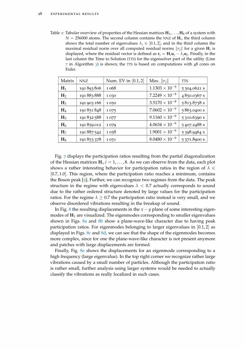
Table 1: Tabular overview of properties of the Hessian matrices H1, . . . , H8 of a system withN = 256000 atoms. The second column contains the NNZ of Hi, the third columnshows the total number of eigenvalues λj ∈ [0.1, 2], and in the third column themaximal residual norm over all computed residual norms ‖rj‖ for a given Hi isdisplayed, where the residual vector is defined as rj = Hiuj − λjuj. Finally, in thelast column the Time to Solution (TTS) for the eigensolver part of the utility (Line7 in Algorithm 3) is shown; the TTS is based on computations with 48 cores onEuler.

Matrix NNZ Num. EV in [0.1, 2] Max. ‖rj‖ TTS

H1 191 893 806 1 068 1.1303× 10−95 304.0621 s

H2 191 883 888 1 030 7.2249× 10−94 850.0367 s

H3 191 903 166 1 050 3.5170× 10−85 813.8738 s

H4 191 851 848 1 075 7.0602× 10−95 863.0400 s

H5 191 832 588 1 077 9.1160× 10−95 310.6390 s

H6 191 859 012 1 079 4.0634× 10−95 407.2488 s

H7 191 887 542 1 058 1.9001× 10−95 398.9464 s

H8 191 853 378 1 051 8.0480× 10−95 371.8900 s

Fig. 7 displays the participation ratios resulting from the partial diagonalizationof the Hessian matrices Hi, i = 1, . . . , 8. As we can observe from the data, each plotshows a rather interesting behavior for participation ratios in the region of λ ∈[0.7, 1.0]. This region, where the participation ratio reaches a minimum, containsthe Boson peak [5]. Further, we can recognize two regimes from the data. The peakstructure in the regime with eigenvalues λ < 0.7 actually corresponds to sounddue to the rather ordered structure denoted by large values for the participationratios. For the regime λ ≥ 0.7 the participation ratio instead is very small, and weobserve disordered vibrations resulting in the breakup of sound.

In Fig. 8 the resulting displacements in the x− y plane of some interesting eigen-modes of H1 are visualized. The eigenmodes corresponding to smaller eigenvaluesshown in Figs. 8a and 8b show a plane-wave-like character due to having peakparticipation ratios. For eigenmodes belonging to larger eigenvalues in [0.1, 2] asdisplayed in Figs. 8c and 8d, we can see that the shape of the eigenmodes becomesmore complex, since for one the plane-wave-like character is not present anymoreand patches with large displacements are formed.

Finally, Fig. 8e shows the displacements for an eigenmode corresponding to ahigh frequency (large eigenvalue). In the top right corner we recognize rather largevibrations caused by a small number of particles. Although the participation ratiois rather small, further analysis using larger systems would be needed to actuallyclassify the vibrations as really localized in such cases.

4.1 eigenmode computations 29

0.0 0.5 1.0 1.5 2.0λ

0.00.10.20.30.40.50.60.70.8

Particip

ation ratio

(a) H1

0.0 0.5 1.0 1.5 2.0λ

0.00.10.20.30.40.50.60.70.80.9

Particip

ation ratio

(b) H2

0.0 0.5 1.0 1.5 2.0λ

0.00.10.20.30.40.50.60.70.8

Particip

ation ratio

(c) H3

0.0 0.5 1.0 1.5 2.0λ

0.00.10.20.30.40.50.60.70.8

Particip

ation ratio

(d) H4

0.0 0.5 1.0 1.5 2.0λ

0.00.10.20.30.40.50.60.70.8

Particip

ation ratio

(e) H5

0.0 0.5 1.0 1.5 2.0λ

0.00.10.20.30.40.50.60.70.8

Particip

ation ratio

(f) H6

0.0 0.5 1.0 1.5 2.0λ

0.00.10.20.30.40.50.60.70.8

Particip

ation ratio

(g) H7

0.0 0.5 1.0 1.5 2.0λ

0.00.10.20.30.40.50.60.70.8

Particip

ation ratio

(h) H8

Figure 7: Eigenvalues λ ∈ [0.1, 2.0] of the different samples Hi, i = 1, 2, . . . , 8 plottedagainst the participation ratios.

30 experimental results

0.0 10.0 20.0 30.0 40.0 50.0X

0.0

10.0

20.0

30.0

40.0

50.0

Y

λ = 0.12741644, PR = 0.73054716

(a)

0.0 10.0 20.0 30.0 40.0 50.0X

0.0

10.0

20.0

30.0

40.0

50.0

Y

λ = 0.25767827, PR = 0.69459376

(b)

0.0 10.0 20.0 30.0 40.0 50.0X

0.0

10.0

20.0

30.0

40.0

50.0

Y

λ = 1.72251517, PR = 0.12178708

(c)

0.0 10.0 20.0 30.0 40.0 50.0X

0.0

10.0

20.0

30.0

40.0

50.0

Y

λ = 1.36765677, PR = 0.06610449

(d)

0.0 10.0 20.0 30.0 40.0 50.0X

0.0

10.0

20.0

30.0

40.0

50.0

Y

λ = 1003.35399077, PR = 0.00000678

(e)

Figure 8: Displacement plots for different eigenmodes of H1. The plots show a cut alongthe x − y plane (δz = 0.15 Å) containing the particle with the largest displace-ment. The arrows are proportional to the displacements of the particles, and thedisplacements have been magnified ×300 for visibility reasons.

4.2 performance measurements 31

4.2 performance measurements

4.2.1 Experimental Setup

All the performance measurements were carried out on the Ra cluster2 at PSI. Thecluster itself consists of 32 nodes, of which 16 are equipped with 2 Intel Xeon E5-2690v3 (2.60 GHz) processors, each providing 12 cores, for a total of 24 cores pernode. The other 16 nodes are equipped with 2 Intel Xeon E5-2697Av4 (2.60 GHz)processors, each processor providing 16 cores, resulting in 32 cores per node. Ourperformance measurements were run on four nodes that are part of the latter 16

nodes, thus allowing to perform measurements with up to 128 cores.Our performance tests have been compiled with GCC 6.2.0 and the following

optimization flags:

-ftree-vectorize -march=core-avx2 -mavx2 -std=c++11 -O3

Further, the following libraries were used: OpenMPI 1.10.4, HDF5 1.8.18, Boost1.62.0, and Trilinos 12.10.1.

The performance measurements are all based on computations with a Hessianmatrix H1 of dimension n1 = 96 000 with nnz = 23 985 126 non-zero elements.

The data shown in the speedup, parallel efficiency, strong scaling and weakscaling plots for our implementations are based on the average time over 10 runs ofa given computation on a given number of cores. Further, 2 warm-up computationsare run before the beginning of the actual measurements. This procedure avoidscomputations on an empty (“cold”) cache, ensuring that after the first warm-upruns the cache is filled with data, resulting in fewer cache-misses during the firstperformance measurement compared to a cold-cache run.

Finally, all performance measurements presented in this section were carried outon Np = 1, 2, 4, . . . , 128 cores.

4.2.2 Polynomial Filter Operator ρk(H)

For these performance tests we measured the average wall-clock time it takes tocompute the matrix-multivector product

ρk(H1)X (57)

using our distributed implementation of the PFO ρk(H) shown in Algorithm 7,where X ∈ Rn1×b, b is the block size, and H1 is the transformed matrix H1.

4.2.2.1 Speedup and Parallel Efficiency

The speedup Sp is defined to be the ratio

Sp =t1

tp, (58)

2 https://www.psi.ch/photon-science-data-services/offline-computing-facility-for-sls-and-swissfel-data-analysis

32 experimental results

where t1 is the time to execute the workload on one core and tp is the time toexecute the workload on p cores. The speedup can be also written as

Sp =t1

tp=

1fs + fp/p

, (59)

where fs is the serial fraction of a routine, fp the parallel fraction of the sameroutine and p the number of cores.

The parallel efficiency is defined as

Ep =t1

p tp=

Sp

p, (60)

and depicts the speedup per core.Fig. 9 shows the speedup and parallel efficiency of our implementation of Eq.

(57) for an experiment with a large degree k = 500 and block size b = 32, bothparameters being held fixed during the measurements. The green line depicts theideal linear speedup. From the plot shown in Fig. 9 we can infer that the speedupof our implementation is linear, but still less than the ideal speedup. Fig. 10 showsthe speedup and parallel efficiency for the same implementation with k = 151 andb = 128, which shows asymptotically a similar behavior to the previous experimentwith a larger degree k and smaller block size b. Reason for these results is for onethe communication overhead caused by the distributed sparse Matrix-MultivectorMultiplication (spMMM) in Algorithm 7. The distributed spMMM used is the defaultimplemented spMMM in Trilinos based on the row-wise distribution of the data asdefined in Section 3.2.

0 20 40 60 80 100 120 140N_p cores

020406080

100120140

Spee

dup

IdealMeasured

(a) Speedup

0 20 40 60 80 100 120 140N_p cores

0.50.60.70.80.91.01.1

Effic

ienc

y

(b) Parallel efficiency

Figure 9: Measured speedup and parallel efficiency of the polynomial operator implemen-tation with k = 500 and b = 32, with the time measurements being averaged over10 runs.

4.2 performance measurements 33

0 20 40 60 80 100 120 140N_p cores

020406080

100120140

Spee

dup

IdealMeasured

(a) Speedup

0 20 40 60 80 100 120 140N_p cores

0.50.60.70.80.91.01.1

Effic

ienc

y

(b) Parallel efficiency

Figure 10: Measured speedup and parallel efficiency of the matrix-multivector multiplica-tion in Eq. (57) with k = 151 and b = 128, with the time measurements beingaveraged over 10 runs.

4.2.2.2 Strong and Weak Scaling

For the weak scaling measurements of Algorithm 7 the problem size assignedto each core stays constant and additional cores are used to solve a larger totalproblem. In our case, the problem size is depicted either by the block size b of Xor by the polynomial degree k of ρk(H) in Eq. (53), and is scaled linearly with thenumber of cores.

Fig. 11a shows the weak scaling of the matrix-multivector multiplication withincreasing block size. Fig. 11b instead shows the weak scaling with increasing poly-nomial degree. As can be observed from the plots, the weak scaling measurementsshow quite an increase in the time to solution, caused mostly by the previouslymentioned communication overhead from the spMMM with the row-based distribu-tion pattern.

1 2 4 8 16 32 64 128N_p cores

0

10

20

30

40

Time [s]

(a) b = 2 per core and overall fixed k = 151.

1 2 4 8 16 32 64 128N_p cores

012345

Time [s]

(b) k = 5 per core and overall fixed b = 8.

Figure 11: Weak scaling measurements of the matrix-multivector multiplication in Eq. (57)with increasing block size b (left) and increasing polynomial degree k (right).

The strong scaling measurements were carried out by keeping the total block sizeb of X or total polynomial degree k of ρk(H) constant and increasing the number ofcores. Both strong scaling plots shown in Fig. 12a and Fig. 12b respectively displaylinear behavior with increasing number of cores.

34 experimental results

1 2 4 8 16 32 64 128N_p cores

101

102

103

Time [s]

y = -0.84692x + 2.96781

(a) b = 32 and k = 500.

1 2 4 8 16 32 64 128N_p cores

101

102

103

Time [s]

y = -0.85196x + 2.88808

(b) b = 128 and k = 151.

Figure 12: Strong scaling measurements of the matrix-multivector multiplication in Eq.(57). The blue line results from a linear regression using the measured timings.

5C O N C L U S I O N A N D F U T U R E D E V E L O P M E N T S

The goal of this thesis was to compute the eigenpairs of a Hessian matrix H in agiven interior interval of the spectrum close to the Boson peak regime by using apolynomial filtered eigensolver.

We were able to successfully run multiple interval-specific eigenpair computa-tions close to the Boson peak regime involving Hessian matrices H ∈ R768000×768000

of systems with N = 256000 atoms. Our calculations concur with the previous re-sults presented by Derlet et al [5].

With the current implementation of the PFO we managed to measure a maximalspeedup of 68 with 128 cores, which demonstrates that our implementation scalesup with increasing number of cores. Although the speedup behavior is satisfac-tory, our performance investigations show that there is still room for improvement.Since most of the work is done by the spMMM, in a future endeavor it would be ad-vantageous to actually try different parallel distribution patterns and implementthe spMMM based on these patterns. One example of such a distribution pattern isthe two-dimensional block data distribution as shown in e.g. [4].

To actually further study the anomalous behavior around the Boson peak regionof the spectrum, the partial diagonalization of Hessian matrices of systems withmillions of atoms is required, and our current implementation should be able tohandle computations with larger matrices. Nonetheless, with increasing matrix di-mensions the number of eigenpairs to be computed within an interval increasesalso, and thus it would be favorable to further distribute the computational workon a given interval to different ranks based on smaller subintervals. A good spec-trum slicing strategy is to divide the interval based on the distribution of theeigenvalues, which can be accomplished by computing estimations of the Densityof States (DOS) [12, 13]. The methods for spectral density estimation shown in [13]have the common characteristics that they all use a stochastic and averaging tech-nique to obtain an approximate DOS. A very similar technique is used by our par-allel implementation of the estimation of the eigenvalue count [6]. Thus, extendingour implementation with methods for the estimation of the spectral density couldbe accomplished in rather reasonable time.

Computations at the end of the spectrum of a Hessian matrix are also of someinterest for the analysis of the general behavior of particles with increasing systemsizes. In this case, an improved approximation of the extremal eigenvalues wouldbe needed to actually deliver reliable results. The approach presented by Zhou andLi [20] provides tight upper bounds with low cost, and could be very suitable forthe reliable computation of eigenpairs in the extremal regions of the spectrum.

Finally, detailed studies of the distribution of eigenvalues in intervals close tothe Boson peak regime could be beneficial to actually tell more about the accuracyof the computed eigenmodes. Also, depending on the distribution of eigenval-ues, more suitable strategies for the estimation of the spectral density could beemployed, possibly resulting in an improved distribution of interval-specific com-putations for a given interval if needed.

35

AA P P E N D I X A

a.1 user manual : bosonpeak utility

In this section we are going to show the steps to first deploy, then compile, andfinally run the BosonPeak Utility (BPU).

a.1.1 Deploying the BosonPeak Utility on the Euler (ETH Zürich) and/or Ra (PSI) Clus-ter

In a first step, we need to load all the necessary environment variables and pro-gram libraries. In the folder BosonPeak/scripts/cluster_setup two bash scripts canbe found that actually accomplish this task. The script setup-euler.sh actually canbe used to deploy the BPU on the Euler cluster, whereas setup-psi.sh can be usedto do the same on the Ra cluster at PSI.

The scripts can be run with the following command (to be issued on the console):

> source setup-<euler|psi>.sh

where <euler|psi> can be replaced with either euler or psi, i.e., in this case eitherrun source setup-euler.sh or source setup-psi.sh

The source command is important in this scenario, since it will actually load allthe environment variables into the global variable space for the current session.Without the source command the environment variables won’t be loaded correctly,and the compilation later will fail, since it depends on these variables.

a.1.2 Code Compilation

Once the steps in Section A.1.1 have been successfully done, we can move on tocompiling the BPU source code.

First, change into the source code directory:

> cd BosonPeak/src/bosonpeak_utility

The folder contains the following files:

- BosonPeak_Utility.cpp

- CMakeLists.txt

- do-configure-euler.sh

- do-configure-psi.sh

The first file consists of the C++ code of the utility, which we are going to compilelater. CMakeLists.txt contains the project configuration and will be used by CMaketo actually build the project. Finally, the do-configure-*.sh files actually, when run,issue the CMake command and load the necessary Trilinos environment variables.

To actually build all the necessary files for the compilation of the source codewe only need to run the corresponding bash script:

37

38 appendix a

> ./do-configure-<euler|psi>.sh

After this, we can simply compile the source code using multiple cores with

> make -j<nr-cores>

where <nr-cores> can be replaced with the number of cores to use for compilingthe code. If the compilation was successful, you can find the resulting binary inthe bin folder of the same directory (or simply as an absolute path: BosonPeak/src/bosonpeak_utility/bin/bosonpeak_utility). This is the executable we are going touse later to actually run different computations.

a.1.3 Configuring the BosonPeak Utility to Run Different Calculations

The XML configuration file contains all the necessary configuration parameters torun different computations, be it an approximation of the extremal eigenvalues,the estimation of the eigenvalue count in an interval, or the computation of aspecified number of eigenpairs in an interval. The BPU can then be launched withthe absolute path to the XML configuration file as a parameter:

> cd BosonPeak/src/bosonpeak_utility

> ./bin/bosonpeak_utlity --cf=/path/to/config.xml

a.1.3.1 Estimation of the Extremal Eigenvalues of A

For the estimation of the extremal eigenvalues λmin and λmax of the matrix A wefirst need to specify the path to the HDF5 file containing the matrix entries andwhich of the extremal eigenvalues we want to estimate. If we actually alreadyknow the extremal eigenvalues, we can simply specify them with the parameterlist Spectrum Boundaries Approximation as shown in Listing 1.

Listing 1: Configuration of the extremal eigenvalues to be used for the transformation ofthe matrix as defined in Eq. (6).

<ParameterList name="BosonPeak Configuration">

<Parameter name="Verbose" type="bool" value="1" />

<ParameterList name="Matrix Import">

<Parameter name="Path to Matrix HDF5 File" type="string" value="/

cluster/matrix.h5"/>

</ParameterList>

<ParameterList name="Spectrum Boundaries Approximation">

<Parameter name="LambdaMin" type="double" value="0.0" />

<Parameter name="LambdaMax" type="double" value="3.0" />

</ParameterList>

</ParameterList>

If we want to estimate both or just a single extremal eigenvalue, we can specifythe Spectrum Boundaries Approximation parameter list (Listing 1) and leave out theeigenvalues we want to estimate. The utility will then estimate the extremal eigen-values based on the missing specifications in the Spectrum Boundaries Approximation

parameter list.By default we run 10 iterations of the Lanczos algorithm for the estimation of

the required extremal eigenvalues. If we wish to use a larger number of Lanczos

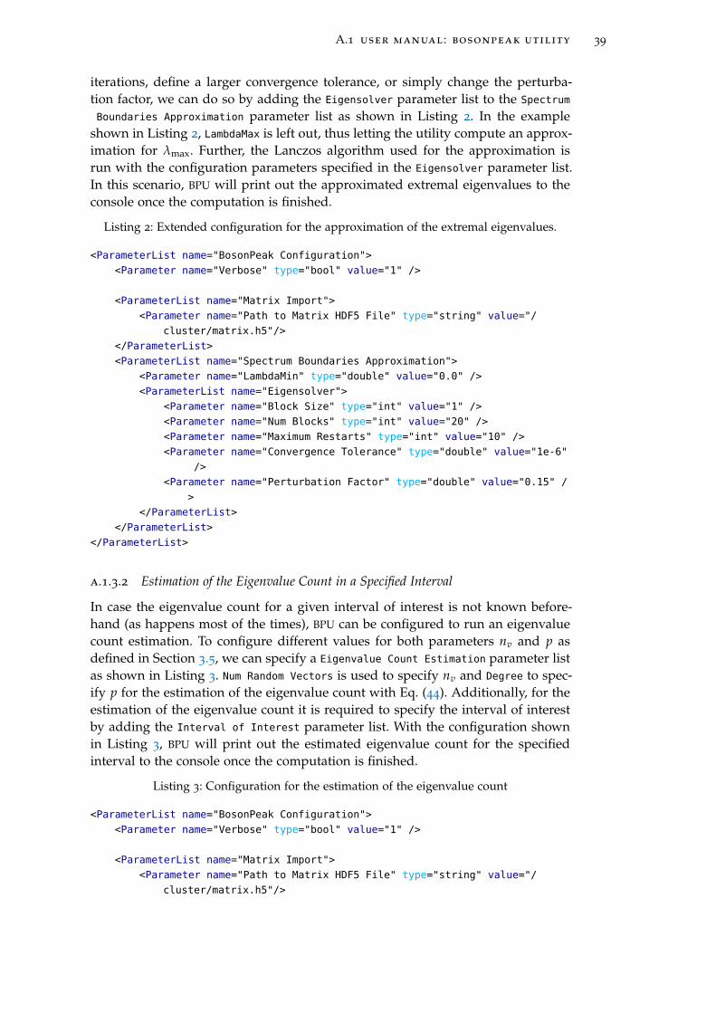
A.1 user manual : bosonpeak utility 39

iterations, define a larger convergence tolerance, or simply change the perturba-tion factor, we can do so by adding the Eigensolver parameter list to the Spectrum

Boundaries Approximation parameter list as shown in Listing 2. In the exampleshown in Listing 2, LambdaMax is left out, thus letting the utility compute an approx-imation for λmax. Further, the Lanczos algorithm used for the approximation isrun with the configuration parameters specified in the Eigensolver parameter list.In this scenario, BPU will print out the approximated extremal eigenvalues to theconsole once the computation is finished.

Listing 2: Extended configuration for the approximation of the extremal eigenvalues.

<ParameterList name="BosonPeak Configuration">

<Parameter name="Verbose" type="bool" value="1" />

<ParameterList name="Matrix Import">

<Parameter name="Path to Matrix HDF5 File" type="string" value="/

cluster/matrix.h5"/>

</ParameterList>

<ParameterList name="Spectrum Boundaries Approximation">

<Parameter name="LambdaMin" type="double" value="0.0" />

<ParameterList name="Eigensolver">

<Parameter name="Block Size" type="int" value="1" />

<Parameter name="Num Blocks" type="int" value="20" />

<Parameter name="Maximum Restarts" type="int" value="10" />

<Parameter name="Convergence Tolerance" type="double" value="1e-6"

/>

<Parameter name="Perturbation Factor" type="double" value="0.15" /

>

</ParameterList>

</ParameterList>

</ParameterList>

a.1.3.2 Estimation of the Eigenvalue Count in a Specified Interval

In case the eigenvalue count for a given interval of interest is not known before-hand (as happens most of the times), BPU can be configured to run an eigenvaluecount estimation. To configure different values for both parameters nv and p asdefined in Section 3.5, we can specify a Eigenvalue Count Estimation parameter listas shown in Listing 3. Num Random Vectors is used to specify nv and Degree to spec-ify p for the estimation of the eigenvalue count with Eq. (44). Additionally, for theestimation of the eigenvalue count it is required to specify the interval of interestby adding the Interval of Interest parameter list. With the configuration shownin Listing 3, BPU will print out the estimated eigenvalue count for the specifiedinterval to the console once the computation is finished.

Listing 3: Configuration for the estimation of the eigenvalue count

<ParameterList name="BosonPeak Configuration">

<Parameter name="Verbose" type="bool" value="1" />

<ParameterList name="Matrix Import">

<Parameter name="Path to Matrix HDF5 File" type="string" value="/

cluster/matrix.h5"/>

40 appendix a

</ParameterList>

<ParameterList name="Spectrum Boundaries Approximation">

<Parameter name="LambdaMin" type="double" value="0.0" />

<Parameter name="LambdaMax" type="double" value="3.0" />

</ParameterList>

<ParameterList name="Interval of Interest">

<Parameter name="Interval Start" type="double" value="0.1" />

<Parameter name="Interval End" type="double" value="1" />

</ParameterList>

<ParameterList name="Eigenvalue Count Estimation">

<Parameter name="Num Random Vectors" type="int" value="40"/>

<Parameter name="Degree" type="int" value="100"/>

</ParameterList>

</ParameterList>

a.1.3.3 Eigensolver Configuration

Once we have estimations for the extremal eigenvalues and an estimated numberof eigenvalues in the interval of interest, we are ready to run eigenpair compu-tations in the specific interval. An example of such a configuration is shown inListing 4. Once the computation has finished, files containing the computed eigen-values, eigenvectors and norms of all residuals will be written to the location spec-ified by the Path to Output Folder parameter. The files are all stored in the MM fileformat.

Listing 4: Complete configuration for the computation of eigenpairs in a specific intervalof the spectrum.

<ParameterList name="BosonPeak Configuration">

<Parameter name="Verbose" type="bool" value="1" />

<ParameterList name="Matrix Import">

<Parameter name="Path to Matrix HDF5 File" type="string" value="/

cluster/matrix.h5"/>

</ParameterList>

<ParameterList name="Spectrum Boundaries Approximation">

<Parameter name="LambdaMin" type="double" value="0.0" />

<Parameter name="LambdaMax" type="double" value="1919.756431988085296"

/>

</ParameterList>

<ParameterList name="Interval of Interest">

<Parameter name="Interval Start" type="double" value="0.0" />

<Parameter name="Interval End" type="double" value="3.0" />

</ParameterList>

<ParameterList name="Filter Polynomial Computation">

<Parameter name="Min Degree" type="int" value="2"/>

<Parameter name="Max Degree" type="int" value="1000"/>

<Parameter name="Smoother" type="string" value="Jackson"/>

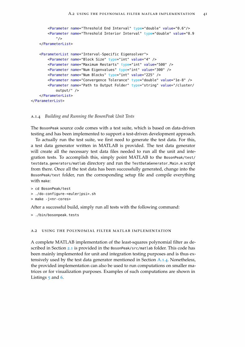
A.2 using the polynomial filter matlab implementation 41

<Parameter name="Threshold End Interval" type="double" value="0.6"/>

<Parameter name="Threshold Interior Interval" type="double" value="0.9

"/>

</ParameterList>

<ParameterList name="Interval-Specific Eigensolver">

<Parameter name="Block Size" type="int" value="4" />

<Parameter name="Maximum Restarts" type="int" value="500" />

<Parameter name="Num Eigenvalues" type="int" value="300" />

<Parameter name="Num Blocks" type="int" value="225" />

<Parameter name="Convergence Tolerance" type="double" value="1e-8" />

<Parameter name="Path to Output Folder" type="string" value="/cluster/

output/" />

</ParameterList>

</ParameterList>

a.1.4 Building and Running the BosonPeak Unit Tests

The BosonPeak source code comes with a test suite, which is based on data-driventesting and has been implemented to support a test-driven development approach.

To actually run the test suite, we first need to generate the test data. For this,a test data generator written in MATLAB is provided. The test data generatorwill create all the necessary test data files needed to run all the unit and inte-gration tests. To accomplish this, simply point MATLAB to the BosonPeak/test/

testdata_generators/matlab directory and run the TestDataGenerator_Main.m scriptfrom there. Once all the test data has been successfully generated, change into theBosonPeak/test folder, run the corresponding setup file and compile everythingwith make:

> cd BosonPeak/test

> ./do-configure-<euler|psi>.sh

> make -j<nr-cores>

After a successful build, simply run all tests with the following command:

> ./bin/bosonpeak_tests

a.2 using the polynomial filter matlab implementation

A complete MATLAB implementation of the least-squares polynomial filter as de-scribed in Section 2.1 is provided in the BosonPeak/src/matlab folder. This code hasbeen mainly implemented for unit and integration testing purposes and is thus ex-tensively used by the test data generator mentioned in Section A.1.4. Nonetheless,the provided implementation can also be used to run computations on smaller ma-trices or for visualization purposes. Examples of such computations are shown inListings 5 and 6.

42 appendix a

Listing 5: Example code showing the usage of the MATLAB implementation of the poly-nomial filter for the computation of eigenvalues in a specific interval of interest.We are using a simple diagonal matrix A with spectrum σ = {1, 2, 3, 4, . . . , 20}and compute all the eigenvalues λi in the interval [11.5, 14.2]. Before runningthis code it is important to first load all the necessary environment variables byrunning the setup-<euler|psi>.sh script as described in Section A.1.1.

BOSONPEAK_MATLAB_SOURCE_DIR = ’BOSONPEAK_MATLAB_SOURCE_DIR’;

addpath(strcat(getenv(BOSONPEAK_MATLAB_SOURCE_DIR), ’/’));

addpath(strcat(getenv(BOSONPEAK_MATLAB_SOURCE_DIR), ’/constants’));

addpath(strcat(getenv(BOSONPEAK_MATLAB_SOURCE_DIR), ’/types’));

% Specify some example spectrum boundaries

lambda_min = 1;

lambda_max = 20;

% Define a simple diagonal matrix

matrix_A = diag((lambda_min:lambda_max));

% Polynomial filter configuration

min_degree = 2;

max_degree = 300;

smoother = BosonPeak_SmootherType.JACKSON;

threshold_interior_interval = 0.6;

threshold_end_interval = 0.3;

% We want to compute all the eigenpairs in the

% interval of interest [11.5, 17.2]

interval_start = 11.5;

interval_end = 14.2;

% Compute the polynomial filter

[gamma_, bar_value, optimal_degree, expansion_coefficients] =

computeFilterPolynomial(lambda_min, lambda_max, interval_start,

interval_end, min_degree, max_degree, smoother,

threshold_interior_interval, threshold_end_interval);

fprintf(’\n=======================================\n’);

fprintf(’Configuration of polynomial filter\n’);

fprintf(’-----------------------------------------\n’);

fprintf(’gamma_ = %.15f\n’, gamma_);

fprintf(’bar_value = %.15f\n’, bar_value);

fprintf(’optimal_degree = %d\n’, optimal_degree);

fprintf(’=========================================\n’);

% Compute the scaling factors and transform the matrix H

[c,d] = computeScalingFactors(lambda_min, lambda_max);

matrix_A_hat = transformMatrix(matrix_A, c, d);

% Compute the matrix rho_k(A_hat) by using the

% Chebyshev three-term recurrence and the computed

% polynomial filter parameters

T_jm2 = eye(size(matrix_A_hat));

T_jm1 = matrix_A_hat;

rho_matrix_A_hat_0 = expansion_coefficients(1) * T_jm2;

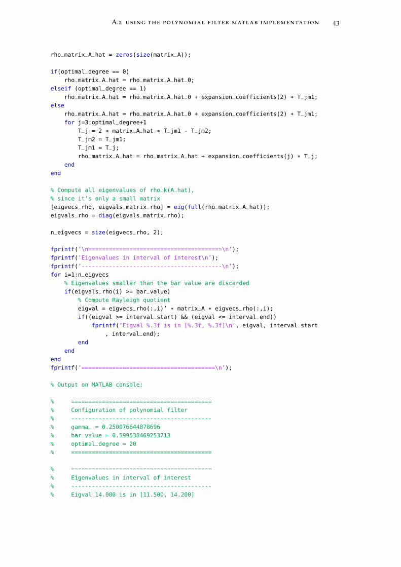
A.2 using the polynomial filter matlab implementation 43

rho_matrix_A_hat = zeros(size(matrix_A));

if(optimal_degree == 0)

rho_matrix_A_hat = rho_matrix_A_hat_0;

elseif (optimal_degree == 1)

rho_matrix_A_hat = rho_matrix_A_hat_0 + expansion_coefficients(2) * T_jm1;

else

rho_matrix_A_hat = rho_matrix_A_hat_0 + expansion_coefficients(2) * T_jm1;

for j=3:optimal_degree+1

T_j = 2 * matrix_A_hat * T_jm1 - T_jm2;

T_jm2 = T_jm1;

T_jm1 = T_j;

rho_matrix_A_hat = rho_matrix_A_hat + expansion_coefficients(j) * T_j;

end

end

% Compute all eigenvalues of rho_k(A_hat),

% since it’s only a small matrix

[eigvecs_rho, eigvals_matrix_rho] = eig(full(rho_matrix_A_hat));

eigvals_rho = diag(eigvals_matrix_rho);

n_eigvecs = size(eigvecs_rho, 2);

fprintf(’\n=======================================\n’);

fprintf(’Eigenvalues in interval of interest\n’);

fprintf(’-----------------------------------------\n’);

for i=1:n_eigvecs

% Eigenvalues smaller than the bar value are discarded

if(eigvals_rho(i) >= bar_value)

% Compute Rayleigh quotient

eigval = eigvecs_rho(:,i)’ * matrix_A * eigvecs_rho(:,i);

if((eigval >= interval_start) && (eigval <= interval_end))

fprintf(’Eigval %.3f is in [%.3f, %.3f]\n’, eigval, interval_start

, interval_end);

end

end

end

fprintf(’=======================================\n’);

% Output on MATLAB console:

% =========================================

% Configuration of polynomial filter

% -----------------------------------------

% gamma_ = 0.250076644878696

% bar_value = 0.599538469253713

% optimal_degree = 20

% =========================================

% =========================================

% Eigenvalues in interval of interest

% -----------------------------------------

% Eigval 14.000 is in [11.500, 14.200]

44 appendix a

% Eigval 12.000 is in [11.500, 14.200]

% Eigval 13.000 is in [11.500, 14.200]

% =========================================

Listing 6: Example code showing the usage of the MATLAB implementation of the polyno-mial filter for the visualization of the resulting filter. Fig. 13 shows the resultingplot from this code. Before running this code it is important to first load all thenecessary environment variables by running the setup-<euler|psi>.sh scriptas described in Section A.1.1.

BOSONPEAK_MATLAB_SOURCE_DIR = ’BOSONPEAK_MATLAB_SOURCE_DIR’;

addpath(strcat(getenv(BOSONPEAK_MATLAB_SOURCE_DIR), ’/’));

addpath(strcat(getenv(BOSONPEAK_MATLAB_SOURCE_DIR), ’/constants’));

addpath(strcat(getenv(BOSONPEAK_MATLAB_SOURCE_DIR), ’/types’));

% Specify some example spectrum boundaries

lambda_min = 1;

lambda_max = 20;

% Polynomial filter configuration

min_degree = 2;

max_degree = 300;

smoother = BosonPeak_SmootherType.JACKSON;

threshold_interior_interval = 0.6;

threshold_end_interval = 0.3;

% We want to compute all the eigenpairs in the

% interval of interest [11.5, 17.2]

interval_start = 11.5;

interval_end = 14.2;

% Compute the polynomial filter

[gamma_, bar_value, optimal_degree, expansion_coefficients] =

computeFilterPolynomial(lambda_min, lambda_max, interval_start,

interval_end, min_degree, max_degree, smoother,

threshold_interior_interval, threshold_end_interval);

% Plotting setup

n_x = 100;

% Define the data points where the polynomial filter should be

% evaluated

x = linspace(BosonPeak_Constants.REFERENCE_INTERVAL_LEFT_ENDPOINT_VALUE,

BosonPeak_Constants.REFERENCE_INTERVAL_RIGHT_ENDPOINT_VALUE, n_x);

% Vector containing the values of the polynomial filter evaluated at

% each point contained in x

rho_x = zeros(1, n_x);

for i=1:n_x

rho_x(i) = evalRho(x(i), optimal_degree, expansion_coefficients);

end

% Compute the scaling factors and transform the boundaries of the

% interval of interest

[c,d] = computeScalingFactors(lambda_min, lambda_max);

A.3 converting mm files storing large symmetric matrices to trilinos compatible hdf5 files 45

interval_start_hat = (interval_start - c) / d;

interval_end_hat = (interval_end - c) / d;

polynomial_filter_plot = figure;

set(gca,’fontsize’,16)

hold on;

endpoint_offset = 0.2;

min_rho_x = 0;

max_rho_x = 1;

xlim([BosonPeak_Constants.REFERENCE_INTERVAL_LEFT_ENDPOINT_VALUE -

endpoint_offset, BosonPeak_Constants.

REFERENCE_INTERVAL_RIGHT_ENDPOINT_VALUE + endpoint_offset]);

ylim([min_rho_x - endpoint_offset, max_rho_x + endpoint_offset]);

xlabel(’$\hat\lambda$’,’Interpreter’,’LaTex’);

ylabel(’$\rho(\hat\lambda)$’,’Interpreter’,’LaTex’);

line([interval_start_hat interval_start_hat], [min_rho_x, max_rho_x], ’Color’,

’red’,’LineStyle’,’--’, ’LineWidth’, 2);

line([interval_end_hat interval_end_hat], [min_rho_x, max_rho_x], ’Color’,’red

’,’LineStyle’,’--’, ’LineWidth’, 2);

plot(x, rho_x, ’-’, ’Color’, ’blue’, ’LineWidth’, 2);

-1 -0.5 0 0.5 1-0.2

0

0.2

0.4

0.6

0.8

1

1.2

Figure 13: Polynomial filter ρk (Eq. (5)) computed and plotted by using the MATLAB codedisplayed in Listing 6.

a.3 converting mm files storing large symmetric matrices to trili-nos compatible hdf5 files

As part of this project, the Hessian matrices were provided in the symmetric MM

format. To actually import such a matrix via BPU we first have to convert the

46 appendix a

MM file to a Trilinos compatible HDF5 file. This is accomplished by using theconvert_mm_matrix_to_hdf5.py script located in the BosonPeak/scripts/matrix_converter

directory. Just specify the path to the source file containing the matrix entries inthe symmetric MM format and the path to the destination HDF5 file:

> cd BosonPeak/scripts/matrix_converter

> python convert_mm_matrix_to_hdf5.py /source/matrix.mm /destination/matrix.

hdf5

Since we want to be able to convert very large files (up to hundreds of Gigabytes),we implemented a buffered conversion approach to avoid overflowing the mainmemory, meaning that we only load and convert small data chunks at a time. Thesize of the data chunks can be specified by supplying the Python script with athird parameter, namely the size of the data chunks in Bytes:

> python convert_mm_matrix_to_hdf5.py /source/matrix.mm /destination/matrix.

hdf5 1000000

In the above example, the script will be loading and converting 1 Megabyte of dataat a time.

B I B L I O G R A P H Y

[1] Haim Avron and Sivan Toledo. “Randomized algorithms for estimating thetrace of an implicit symmetric positive semi-definite matrix.” In: Journal ofthe ACM 58.2 (2011), p. 8.

[2] Costas Bekas, Effrosyni Kokiopoulou, and Yousef Saad. “An estimator for thediagonal of a matrix.” In: Applied numerical mathematics 57.11 (2007), pp. 1214–1229.

[3] YM Beltukov, C Fusco, DA Parshin, and A Tanguy. “Boson peak and Ioffe-Regel criterion in amorphous siliconlike materials: The effect of bond direc-tionality.” In: Physical Review E 93.2 (2016), p. 023006.

[4] Aydin Buluç and John R Gilbert. “Parallel sparse matrix-matrix multiplica-tion and indexing: Implementation and experiments.” In: SIAM Journal onScientific Computing 34.4 (2012), pp. C170–C191.

[5] PM Derlet, R Maaß, and JF Löffler. “The Boson peak of model glass sys-tems and its relation to atomic structure.” In: The European Physical JournalB-Condensed Matter and Complex Systems 85.5 (2012), pp. 1–20.

[6] Edoardo Di Napoli, Eric Polizzi, and Yousef Saad. “Efficient estimation ofeigenvalue counts in an interval.” In: Numerical Linear Algebra with Applica-tions 23.4 (2016), pp. 674–692.

[7] Haw-ren Fang and Yousef Saad. “A filtered Lanczos procedure for extremeand interior eigenvalue problems.” In: SIAM Journal on Scientific Computing34.4 (2012), A2220–A2246.

[8] Michael F Hutchinson. “A stochastic estimator of the trace of the influencematrix for Laplacian smoothing splines.” In: Communications in Statistics-Simulation and Computation 19.2 (1990), pp. 433–450.

[9] Laurent O Jay, Hanchul Kim, Yousef Saad, and James R Chelikowsky. “Elec-tronic structure calculations for plane-wave codes without diagonalization.”In: Computer physics communications 118.1 (1999), pp. 21–30.

[10] Cornelius Lanczos. An iteration method for the solution of the eigenvalue problemof linear differential and integral operators. United States Governm. Press OfficeLos Angeles, CA, 1950.

[11] Cornelius Lanczos. Applied analysis. Dover Publications, 1988.

[12] Ruipeng Li, Yuanzhe Xi, Eugene Vecharynski, Chao Yang, and Yousef Saad.“A Thick-Restart Lanczos algorithm with polynomial filtering for Hermitianeigenvalue problems.” In: SIAM Journal on Scientific Computing 38.4 (2016),A2512–A2534.

[13] Lin Lin, Yousef Saad, and Chao Yang. “Approximating spectral densities oflarge matrices.” In: SIAM Review 58.1 (2016), pp. 34–65.

[14] Theodore J Rivlin. An introduction to the approximation of functions. BlaisdellPublishing Company, 1969.

47

48 Bibliography

[15] Yousef Saad. Numerical methods for large eigenvalue problems. Manchester Uni-versity Press, 1992.

[16] Yousef Saad, Ruipeng Li, Yuanzhe Xi, Luke Erlandson, Eugene Vecharinsky,and Chao Yang. EVSL: EigenValues Slicing Library. http://www-users.cs.umn.edu/~saad/software/EVSL/. 2016 – 2017.

[17] Gilbert W Stewart. “A Krylov–Schur algorithm for large eigenproblems.” In:SIAM Journal on Matrix Analysis and Applications 23.3 (2002), pp. 601–614.

[18] Kesheng Wu and Horst Simon. “Thick-restart Lanczos method for large sym-metric eigenvalue problems.” In: SIAM Journal on Matrix Analysis and Appli-cations 22.2 (2000), pp. 602–616.

[19] Ichitaro Yamazaki, Zhaojun Bai, Horst Simon, Lin-Wang Wang, and KeshengWu. “Adaptive projection subspace dimension for the thick-restart Lanczosmethod.” In: ACM Transactions on Mathematical Software (TOMS) 37.3 (2010),p. 27.

[20] Yunkai Zhou and Ren-Cang Li. “Bounding the spectrum of large Hermitianmatrices.” In: Linear Algebra and its Applications 435.3 (2011), pp. 480–493.