solving sat and sat modulo theories: from an abstract ...oliveras/espai/papers/jacm.pdf · solving...
TRANSCRIPT

Solving SAT and SAT Modulo Theories: From an Abstract
Davis–Putnam–Logemann–Loveland Procedure to DPLL(T)
ROBERT NIEUWENHUIS AND ALBERT OLIVERAS
Technical University of Catalonia, Barcelona, Spain
AND
CESARE TINELLI
The University of Iowa, Iowa City, Iowa
Abstract. We first introduce Abstract DPLL, a rule-based formulation of the Davis–Putnam–Logemann–Loveland (DPLL) procedure for propositional satisfiability. This abstract framework al-lows one to cleanly express practical DPLL algorithms and to formally reason about them in a simpleway. Its properties, such as soundness, completeness or termination, immediately carry over to themodern DPLL implementations with features such as backjumping or clause learning.
We then extend the framework to Satisfiability Modulo background Theories (SMT) and use it tomodel several variants of the so-called lazy approach for SMT. In particular, we use it to introduce afew variants of a new, efficient and modular approach for SMT based on a general DPLL(X ) engine,whose parameter X can be instantiated with a specialized solver SolverT for a given theory T , thusproducing a DPLL(T ) system. We describe the high-level design of DPLL(X ) and its cooperationwith SolverT , discuss the role of theory propagation, and describe different DPLL(T ) strategies forsome theories arising in industrial applications.
Our extensive experimental evidence, summarized in this article, shows that DPLL(T ) systemscan significantly outperform the other state-of-the-art tools, frequently even in orders of magnitude,and have better scaling properties.
Categories and Subject Descriptors: B.6.3 [Logic Design]: Design Aids—Verification; F.4.1 [Math-ematical Logic and Formal Languages]: Mathematical Logic—Computational logic; verification;I.2.3 [Artificial Intelligence]: Deduction and Theorem Proving—Deduction (e.g., natural, rule-based)
General Terms: Theory, Verification
Additional Key Words and Phrases: SAT solvers, Satisfiability Modulo Theories
This work was partially supported by Spanish Ministry of Education and Science through the LogicTools project TIN2004-03382 (all authors), the FPU grant AP2002-3533 (Oliveras) and NationalScience Foundation (NSF) grant 0237422 (Tinelli and Oliveras).Authors’ addresses: R. Nieuwenhuis and A. Oliveras, Technical University of Catalonia, CampusNord—Edif. Omega, C. Jordi Girona, 1–3, 08034 Barcelona, Spain; C. Tinelli, University of Iowa,Department of Computer Science, 14 MacLean Hall, Iowa City, IA, 52242.Permission to make digital or hard copies of part or all of this work for personal or classroom use isgranted without fee provided that copies are not made or distributed for profit or direct commercialadvantage and that copies show this notice on the first page or initial screen of a display along with thefull citation. Copyrights for components of this work owned by others than ACM must be honored.Abstracting with credit is permitted. To copy otherwise, to republish, to post on servers, to redistributeto lists, or to use any component of this work in other works requires prior specific permission and/ora fee. Permissions may be requested from Publications Dept., ACM, Inc., 2 Penn Plaza, Suite 701,New York, NY 10121-0701 USA, fax +1 (212) 869-0481, or [email protected]© 2006 ACM 0004-5411/06/1100-0937 $5.00
Journal of the ACM, Vol. 53, No. 6, November 2006, pp. 937–977.

938 R. NIEUWENHUIS ET AL.
1. Introduction
The problem of deciding the satisfiability of propositional formulas (SAT) doesnot only lie at the heart of the most important open problem in complexity theory(P vs. NP), it is also at the basis of many practical applications in such areas as Elec-tronic Design Automation, Verification, Artificial Intelligence, and Operations Re-search. Thanks to recent advances in SAT-solving technology, propositional solversare becoming the tool of choice for attacking more and more practical problems.
Most state-of-the-art SAT solvers [Moskewicz et al. 2001; Goldberg and Novikov2002; Een and Sorensson 2003; Ryan 2004] today are based on different vari-ations of the Davis-Putnam-Logemann-Loveland (DPLL) procedure [Davis andPutnam 1960; Davis et al. 1962]. Starting essentially with the work on theGRASP, SATO and Relsat systems [Marques-Silva and Sakallah 1999; Zhang1997; Bayardo and Schrag 1997], the spectacular improvements in the perfor-mance of DPLL-based SAT solvers achieved in the last years are due to (i) bet-ter implementation techniques, such as the two-watched literal approach for unitpropagation, and (ii) several conceptual enhancements on the original DPLL pro-cedure, aimed at reducing the amount of explored search space, such as backjump-ing (a form of non-chronological backtracking), conflict-driven lemma learning,and restarts. These advances make it now possible to decide the satisfiabilityof industrial SAT problems with tens of thousands of variables and millionsof clauses.
Because of their success, both the DPLL procedure and its enhancements havebeen adapted to handle satisfiability problems in more expressive logics thanpropositional logic. In particular, they have been used to build efficient algo-rithms for the Satisfiability Modulo Theories (SMT) problem: deciding the sat-isfiability of ground first-order formulas with respect to background theories suchas the theory of equality, of the integer or real numbers, of arrays, and so on[Armando et al. 2000, 2004; Filliatre et al. 2001; Barrett et al. 2002; de Mouraand Rueß 2002; Flanagan et al. 2003; Ganzinger et al. 2004; Bozzano et al. 2005].SMT problems arise in many industrial applications, especially in formal verifi-cation (see Section 3 for examples). They may contain thousands of clauses likep ∨ ¬q ∨ a = f (b − c) ∨ g(g(b)) �=c ∨ a − c ≤7, with purely propositional atomsas well as atoms over (combined) theories, such as the theory of the integers, or ofEquality with Uninterpreted Functions (EUF).
Altogether, many variants and extensions of the DPLL procedure exist today.They are typically described in the literature informally and with the aid of pseudo-code fragments. Therefore, it has become difficult for the newcomer to understandthe precise nature of all these procedures, and for the expert to formally reasonabout their properties.
The first main contribution of this article is to address these shortcomings byproviding Abstract DPLL, a uniform, declarative framework for describing DPLL-based solvers, both for propositional satisfiability and for satisfiability modulotheories. The framework allows one to describe the essence of various prominentapproaches and techniques in terms of simple transition rules and rule applicationstrategies. By abstracting away heuristics and implementation issues, it facilitatesthe understanding of DPLL at a conceptual level as well as its correctness and termi-nation. For DPLL-based SMT approaches, it moreover provides a clean formulationand a basis for comparison of the different approaches.

Solving SAT and SAT Modulo Theories 939
The second main contribution of this article is a new modular architecture forbuilding SMT solvers in practice, called DPLL(T ), and a careful study of theorypropagation, a refinement of SMT methods that can have a crucial impact on theirperformance.
The architecture is based on a general DPLL(X ) engine, whose parameter X canbe instantiated with a specialized solver SolverT for a given theory T , thus producinga system DPLL(T ). Such systems can be implemented extremely efficiently andhave good scaling properties: our Barcelogic implementation of DPLL(T ) won fourdivisions at the 2005 SMT Competition [Barrett et al. 2005] (for the other threeexisting divisions it had no SolverT yet). The insights provided by our AbstractDPLL framework were an important factor in the success of our DPLL(T ) archi-tecture and its Barcelogic implementation. For instance, the abstract frameworkhelped us in understanding the interactions between the DPLL(X ) engine and thesolvers, especially concerning the different forms of theory propagation, as well asin defining a good interface between both.
Section 2 of this article presents the propositional version of Abstract DPLL. Itmodels DPLL procedures by means of simple transition systems. While abstractand declarative in nature, these transition systems can explicitly model the salientconceptual features of state-of-the-art DPLL-based SAT solvers, thus bridging thegap between logic-based calculi for DPLL and actual implementations. Within theAbstract DPLL formalism, we discuss in a clean and uniform way properties such assoundness, completeness, and termination. These properties immediately carry overto modern DPLL implementations with features such as backjumping and learning.
For backjumping systems, for instance, we achieve this by modeling backjumpingby a general rule that encompasses several backtracking strategies—including basicchronological backtracking—and explaining how different systems implement therule. Similarly, we model learning by general rules that show how devices such asconflict graphs are just one possibility for computing new lemmas. We also providea general and simple termination argument for DPLL procedures that does notdepend on an exhaustive enumeration of truth assignments; instead, it relies on anotion of search progress neatly expressing that search advances with the deductionof new unit clauses—the higher up in the search tree the better—which is the veryessence of backjumping.
In Section 3, we go beyond propositional satisfiability, and extend the frameworkto Abstract DPLL Modulo Theories. As in the purely propositional case, this againallows us to express—and formally reason about—a number of current DPLL-basedtechniques for SMT, such as the various variants of the so-called lazy approach[Armando et al. 2000, 2004; Filliatre et al. 2001; Audemard et al. 2002; Barrettet al. 2002; de Moura and Rueß 2002; Flanagan et al. 2003; Ball et al. 2004].
In Section 4, based on the Abstract DPLL Modulo Theories framework, we in-troduce our DPLL(T ) approach for building SMT systems. We first describe twovariants of DPLL(T ), depending on whether theory propagation is done exhaus-tively or not. Once the DPLL(X ) engine has been implemented, this approachbecomes extremely flexible: a DPLL(T ) system for a theory T is obtained by sim-ply plugging in the corresponding theory solver SolverT , which must only be ableto deal with conjunctions of theory literals and conform to a minimal and simpleset of additional requirements. We discuss the design of DPLL(X ) and describehow DPLL(X ) and SolverT cooperate. We also show that practical T -solvers canbe designed to include theory propagation in an efficient way. A nontrivial issue

940 R. NIEUWENHUIS ET AL.
is how to deal with conflict analysis and clause learning adequately in the contextof theory propagation. Different options and possible problems for doing this areanalyzed and discussed in detail in Section 5.
In Section 6, we discuss some experiments with our Barcelogic implementationof DPLL(T ). The results show that it can significantly outperform the best state-of-the-art tools and, in addition, scales up very well.
This article consolidates and improves upon preliminary ideas and results pre-sented at the JELIA [Tinelli 2002], LPAR [Nieuwenhuis and Oliveras 2003;Nieuwenhuis et al. 2005], and CAV [Ganzinger et al. 2004; Nieuwenhuis andOliveras 2005a] conferences.
2. Abstract DPLL in the Propositional Case
We start this section with some formal preliminaries on propositional logic and ontransition systems. Then we introduce several variants of Abstract DPLL and provetheir correctness properties, showing at the same time how the different features ofactual DPLL implementations are modeled by these variants.
2.1. FORMULAS, ASSIGNMENTS, AND SATISFACTION. Let P be a fixed finite setof propositional symbols. If p ∈ P , then p is an atom and p and ¬p are literals ofP . The negation of a literal l, written ¬l, denotes ¬p if l is p, and p if l is ¬p. Aclause is a disjunction of literals l1 ∨· · ·∨ln . A unit clause is a clause consisting of asingle literal. A (CNF) formula is a conjunction of one or more clauses C1∧· · ·∧Cn .When it leads to no ambiguities, we will sometimes also write such a formula inset notation {C1, . . . , Cn}, or simply replace the ∧ connectives by commas.
A (partial truth) assignment M is a set of literals such that {p, ¬p} ⊆ M for nop. A literal l is true in M if l ∈ M , is false in M if ¬l ∈ M , and is undefined in Motherwise. A literal is defined in M if it is either true or false in M . The assignmentM is total over P if no literal of P is undefined in M . A clause C is true in M if atleast one of its literals is in M . It is false in M if all its literals are false in M , and itis undefined in M otherwise. A formula F is true in M , or satisfied by M , denotedM |= F , if all its clauses are true in M . In that case, M is a model of F . If F has nomodels then it is unsatisfiable. If F and F ′ are formulas, we write F |= F ′ if F ′ is truein all models of F . Then, we say that F ′ is entailed by F , or is a logical consequenceof F . If F |= F ′ and F ′ |= F , we say that F and F ′ are logically equivalent.
In what follows, (possibly subscripted or primed) lowercase l always denoteliterals. Similarly, C and D always denote clauses, F and G denote formulas, andM and N denote assignments. If C is a clause l1 ∨ · · · ∨ ln , we sometimes write¬C to denote the formula ¬l1 ∧ · · · ∧ ¬ln .
2.2. STATES AND TRANSITION SYSTEMS IN ABSTRACT DPLL. DPLL can befully described by simply considering that a state of the procedure is either thedistinguished state FailState or a pair of the form M ‖ F , where F is a CNF formula,that is, a finite set of clauses, and M is, essentially, a (partial) assignment.
More precisely, M is a sequence of literals, never containing both a literal andits negation, where each literal has an annotation, a bit that marks it as a decisionliteral (see below) or not. Frequently, we will consider M just as a partial assignment,or as a set or conjunction of literals (and hence as a formula), ignoring both theannotations and the order between its elements.

Solving SAT and SAT Modulo Theories 941
The concatenation of two such sequences will be denoted by simple juxtaposition.When we want to emphasize that a literal l is annotated as a decision literal wewill write it as ld. We will denote the empty sequence of literals (or the emptyassignment) by ∅. We say that a clause C is conflicting in a state M ‖ F, C ifM |= ¬C .
We will model each DPLL procedure by means of a set of states together with abinary relation =⇒ over these states, called the transition relation. As usual, we useinfix notation, writing S =⇒ S′ instead of (S, S′) ∈ =⇒. If S =⇒ S′ we say thatthere is a transition from S to S′. We denote by =⇒∗ the reflexive-transitive closureof =⇒. We call any sequence of transitions of the form S0 =⇒ S1, S1 =⇒ S2, · · ·a derivation, and denote it by S0 =⇒ S1 =⇒ S2 =⇒ · · · . We call any subsequenceof a derivation a subderivation.
In what follows, transition relations will be defined by means of conditionaltransition rules. For a given state S, a transition rule precisely defines whetherthere is a transition from S by this rule and, if so, to which state S′. Such a transitionis called an application step of the rule.
A transition system is a set of transition rules defined over some given set ofstates. Given a transition system R, the transition relation defined by R will bedenoted by =⇒R . If there is no transition from S by =⇒R , we will say that S isfinal with respect to R (examples of a transition system and a final state with respectto it can be found in Definition 2.1 and Example 2.2).
2.3. THE CLASSICAL DPLL PROCEDURE. A very simple DPLL system, faithfulto the classical DPLL algorithm, consists of the following five transition rules. Wegive this system here mainly for explanatory and historical reasons. The informallystated results for it are easily obtained by adapting the more general ones given inSection 2.5.
Definition 2.1. The Classical DPLL system is the transition system Cl consist-ing of the following five transition rules. In this system, the literals added to M byall rules except Decide are annotated as non-decision literals.
UnitPropagate :
M ‖ F, C ∨ l =⇒ M l ‖ F, C ∨ l if
{M |= ¬Cl is undefined in M.
PureLiteral :
M ‖ F =⇒ M l ‖ F if
⎧⎨⎩
l occurs in some clause of F¬l occurs in no clause of Fl is undefined in M.
Decide :
M ‖ F =⇒ M ld ‖ F if
{l or ¬l occurs in a clause of Fl is undefined in M .
Fail :
M ‖ F, C =⇒ FailState if
{M |= ¬CM contains no decision literals.
Backtrack :
M ld N ‖ F, C =⇒ M ¬l ‖ F, C if
{M ld N |= ¬CN contains no decision literals.

942 R. NIEUWENHUIS ET AL.
One can use the transition system Cl for deciding the satisfiability of an inputformula F simply by generating an arbitrary derivation ∅ ‖ F =⇒Cl · · · =⇒Cl Sn ,where Sn is a final state with respect to Cl. The applicability of each of the fiverules is easy to check and, as we will see, their application always leads to finitederivations. Moreover, for every derivation like the above ending in a final stateSn , (i) F is unsatisfiable if, and only if, Sn is FailState, and (ii) if Sn is of the formM ‖ F then M is a model of F . Note that in this Classical DPLL system the secondcomponent of a state remains unchanged, a property that does not hold for the othertransition systems we introduce later.
We now briefly comment on what the different rules do. In the following, if M isa sequence of the form M0 l1 M1 · · · lk Mk , where the li are all the decision literalsin M , we say that the state M ‖ F is at decision level k, and that all the literals ofeach li Mi belong to decision level i .
—UnitPropagate: To satisfy a CNF formula, all its clauses have to be true. Hence, ifa clause of F contains a literal l whose truth value is not defined by the currentassignment M while all the remaining literals of the clause are false, then Mmust be extended to make l true.
—PureLiteral: If a literal l is pure in F , that is, it occurs in F while its negation doesnot, then F is satisfiable only if it has a model that makes l true. Thus, if M doesnot define l it can be extended to make l true.
—Decide: This rule represents a case split. An undefined literal l is chosen fromF , and added to M . The literal is annotated as a decision literal, to denote thatif M l cannot be extended to a model of F then the alternative extension M ¬lmust still be considered. This is done by means of the Backtrack rule.
—Fail: This rule detects a conflicting clause C and produces the FailState statewhenever M contains no decision literals.
—Backtrack: If a conflicting clause C is detected and Fail does not apply, then therule backtracks one decision level, by replacing the most recent decision literal ld
by ¬l and removing any subsequent literals in the current assignment. Note that¬l is annotated as a nondecision literal, since the other possibility l has alreadybeen explored.
Example 2.2. The following is a derivation in the Classical DPLL system, witheach transition annotated by the rule that makes it possible. To improve readabilitywe denote atoms by natural numbers, and negation by overlining.
∅ ‖ 1∨2, 2∨3, 1∨3∨4, 2∨3∨4, 1∨4 =⇒Cl (Decide)1d ‖ 1∨2, 2∨3, 1∨3∨4, 2∨3∨4, 1∨4 =⇒Cl (UnitPropagate)
1d 2 ‖ 1∨2, 2∨3, 1∨3∨4, 2∨3∨4, 1∨4 =⇒Cl (UnitPropagate)1d 2 3 ‖ 1∨2, 2∨3, 1∨3∨4, 2∨3∨4, 1∨4 =⇒Cl (UnitPropagate)
1d 2 3 4 ‖ 1∨2, 2∨3, 1∨3∨4, 2∨3∨4, 1∨4 =⇒Cl (Backtrack)1 ‖ 1∨2, 2∨3, 1∨3∨4, 2∨3∨4, 1∨4 =⇒Cl (UnitPropagate)
1 4 ‖ 1∨2, 2∨3, 1∨3∨4, 2∨3∨4, 1∨4 =⇒Cl (Decide)
1 4 3d ‖ 1∨2, 2∨3, 1∨3∨4, 2∨3∨4, 1∨4 =⇒Cl (UnitPropagate)
1 4 3d
2 ‖ 1∨2, 2∨3, 1∨3∨4, 2∨3∨4, 1∨4

Solving SAT and SAT Modulo Theories 943
The last state of this derivation is final. The (total) assignment in it is a model ofthe formula.
The Davis–Putnam procedure [Davis and Putnam 1960] was originally presentedas a two-phase proof-procedure for first-order logic. The unsatisfiability of a formulawas to be proved by first generating a suitable set of ground instances which then,in the second phase, were shown to be propositionally unsatisfiable.
Subsequent improvements, such as the Davis-Logemann-Loveland procedure ofDavis et al. [1962], mostly focused on the propositional phase. What most authorsnow call the DPLL Procedure is a satisfiability procedure for propositional logicbased on this propositional phase. Originally, this procedure amounted to the depth-first search algorithm with backtracking modeled by our Classical DPLL system.
2.4. MODERN DPLL PROCEDURES. The major modern DPLL-based SATsolvers do not implement the Classical DPLL system. For example, due to effi-ciency reasons the pure literal rule is normally only used as a preprocessing step—hence, we will not consider this rule in the following. Moreover, backjumping, amore general and more powerful backtracking mechanism, is now commonly usedin place of chronological backtracking.
The usefulness of a more sophisticated backtracking mechanism for DPLLsolvers is perhaps best illustrated with another example of derivation in the ClassicalDPLL system.
Example 2.3.
∅ ‖ 1∨2, 3∨4, 5∨6, 6∨5∨2 =⇒B (Decide)
1d ‖ 1∨2, 3∨4, 5∨6, 6∨5∨2 =⇒B (UnitPropagate)
1d 2 ‖ 1∨2, 3∨4, 5∨6, 6∨5∨2 =⇒B (Decide)
1d 2 3d ‖ 1∨2, 3∨4, 5∨6, 6∨5∨2 =⇒B (UnitPropagate)
1d 2 3d 4 ‖ 1∨2, 3∨4, 5∨6, 6∨5∨2 =⇒B (Decide)
1d 2 3d 4 5d ‖ 1∨2, 3∨4, 5∨6, 6∨5∨2 =⇒B (UnitPropagate)
1d 2 3d 4 5d 6 ‖ 1∨2, 3∨4, 5∨6, 6∨5∨2 =⇒B (Backtrack)
1d 2 3d 4 5 ‖ 1∨2, 3∨4, 5∨6, 6∨5∨2
Before the Backtrack step, the clause 6 ∨ 5 ∨ 2 is conflicting: it is false in theassignment 1d 2 3d 4 5d 6. This is a consequence of the unit propagation 2 of thedecision 1d, together with the decision 5d and its unit propagation 6.
Therefore, one can infer that the decision 1d is incompatible with the decision5d, that is, that the given clause set entails 1∨5. Similarly, it also entails 2∨5.
Such entailed clauses are called backjump clauses if their presence would haveallowed a unit propagation at an earlier decision level. This is precisely what back-jumping does: given a backjump clause, it goes back to that level and adds theunit propagated literal. For example, using 2∨5 as a backjump clause, the lastBacktrack step could be replaced by a backjump to a state with first component1d 2 5.
We model all this in the next system with the Backjump rule, of which Backtrackis a particular case. In this rule, the clause C ′ ∨ l ′ is the backjump clause, where l ′

944 R. NIEUWENHUIS ET AL.
is the literal that can be unit propagated (5 in our example). Below we show thatthe rule is effective: a backjump clause can always be found.
Definition 2.4. The Basic DPLL system is the four-rule transition system Bconsisting of the rules UnitPropagate, Decide, Fail from Classical DPLL, and thefollowing Backjump rule:
Backjump :
M ld N ‖ F, C =⇒ M l ′ ‖ F, C if
⎧⎪⎪⎪⎪⎨⎪⎪⎪⎪⎩
M ld N |= ¬C, and there issome clause C ′ ∨ l ′ such that:
F, C |= C ′ ∨ l ′ and M |= ¬C ′,l ′ is undefined in M , andl ′ or ¬l ′ occurs in F or in M ld N .
We call clause C in Backjump the conflicting clause and clause C ′ ∨ l ′ the backjumpclause.
Chronological backtracking, modeled by Backtrack, always undoes the last de-cision l, going back to the previous level and adding ¬l to it. Conflict-drivenbackjumping, as modeled by Backjump, is generally able to backtrack further thanchronological backtracking by analyzing the reasons that produced the conflictingclause. Backjump can frequently undo several decisions at once, going back to alower decision level than the previous level and adding some new literal to thatlower level. It jumps over levels that are irrelevant to the conflict. In the previousexample, it jumps over the decision 3d and its consequence 4, which are totally un-related with the reasons for the falsity of the conflicting clause 6∨5∨2. Moreover,intuitively, the search state 1d 2 5 reached after Backjump is more advanced thanthe state 1d 2 3d 4 5 reached after Backtrack. This notion of “being more advanced”is formalized in Theorem 2.10 below.
We show in the proof of Lemma 2.8 below that the literals of the backjump clausecan always be chosen among the negations of the decision literals—although betterchoices usually exist. When the negations of all the decision literals are includedin the backjump clause, the Backjump rule simulates the Backtrack rule of ClassicalDPLL. We remark that, in fact, Lemma 2.8 shows that, whenever a state M ‖ Fcontains a conflicting clause, either Fail applies, if there are no decision literals inM , or otherwise Backjump applies.
Most modern DPLL implementations make additional use of backjump clauses:they add them to the clause set as learned clauses, also called lemmas, implementingwhat is usually called conflict-driven learning.
In Example 2.3, learning the clause 2 ∨ 5 will allow the application ofUnitPropagate to any state whose assignment contains either 2 or 5. Hence, it willprevent any conflict caused by having both 2 and 5 in M . Reaching such similarconflicts frequently happens in industrial problems having some regular structure,and learning such lemmas has been shown to be very effective in improving per-formance.
Since a lemma is aimed at preventing future similar conflicts, when these conflictsare not very likely to be found again the lemma can be removed. In practice, alemma is removed when its relevance (see, e.g., Bayardo and Schrag [1997]) or itsactivity level drops below a certain threshold; the activity can be, for example, the

Solving SAT and SAT Modulo Theories 945
number of times it becomes a unit or a conflicting clause [Goldberg and Novikov2002].
To model lemma learning and removal we consider the following extension ofthe Basic DPLL system.
Definition 2.5. The DPLL system with learning, denoted by L , consists of thefour transition rules of the Basic DPLL system and the two additional rules:
Learn :
M ‖ F =⇒ M ‖ F, C if
{each atom of C occurs in F or in MF |= C.
Forget :M ‖ F, C =⇒ M ‖ F if
{F |= C.
In any application step of Learn, the clause C is said to be learned if it did notalready belong to F . Similarly, it is said to be forgotten by Forget.
Observe that the Learn rule allows one to add to the current formula F an arbitraryclause C entailed by F , as long as all the atoms of C occur in F or M . This modelsnot only conflict-driven lemma learning but also any other techniques that produceconsequences of F , such as limited forms of resolution (see the following example).
Similarly, the Forget rule can be used in principle to remove from F any clausethat is entailed by the rest of F , not just those previously added to the clause set byLearn. The applicability of the two rules in their full scope, however, is limited inpractice by the relative cost of determining such entailments in general.
The six rules of the DPLL system with learning model the high-level conceptualstructure of DPLL implementations. These rules will allow us to formally reasonabout properties such as correctness or termination.
Example 2.6. We now show how the Backjump rule can be guided by means ofa conflict graph for finding backjump clauses. In this example we assume a strategythat is followed in most SAT solvers: (i) Decide is applied only if no other BasicDPLL rule is applicable (Theorem 5.2 of Section 5 shows that this is not needed,but here we require it for simplicity) and (ii) after each application of Backjump, thebackjump clause is learned.
Consider a state of the form M ‖ F where, among other clauses, F contains:
9∨6∨7∨8 8∨7∨5 6∨8∨4 4∨1 4∨5∨2 5∨7∨3 1∨2∨3
and M is of the form: . . . 6 . . . 7 . . . 9d 8 5 4 1 2 3.It is easy to see that this state can be reached after the last decision 9d by six
applications of UnitPropagate. For example, 8 is implied by 9, 6, and 7 because ofthe clause 9∨6∨7∨8. A typical DPLL implementation will save the sequence ofpropagated literals and remember for each one of them the clause that caused itspropagation. Now, in the state M ‖ F above the clause 1∨2∨3 is conflicting, sinceM contains 1, 2 and 3. Using the saved information, the DPLL implementation cantrace back the reasons for this conflicting clause. For example, the saved data willshow that 3 was implied by 5 and 7, due to the clause 5∨7∨3. The literal 5 was inturn implied by 8 and 7, and so on.
This way, working backwards from the conflicting clause and in the oppositeorder in which each literal was propagated, it is possible to build the following

946 R. NIEUWENHUIS ET AL.
conflict graph, where the nodes corresponding to the conflicting clause are shown ingray:
This figure shows the graph obtained when the decision literal of the currentdecision level (here, 9d) is reached in this backwards process—which is why thisnode and the nodes belonging to earlier decision levels (in this example, literals 6and 7) have no incoming arrows.
To find a backjump clause, it suffices to cut the graph into two parts. The firstpart must contain (at least) all the literals with no incoming arrows. The second partmust contain (at least) all the literals with no outgoing arrows, that is, the negatedliterals of the conflicting clause (in our example, 1, 2 and 3). It is not hard to see thatin such a cut no model of F can satisfy all the literals whose outgoing edges are cut.
For instance, consider the cut indicated by the dotted line in the graph, wherethe literals with cut outgoing edges are 8, 7, and 6. From these three literals, byunit propagation using five clauses of F , one can infer the negated literals ofthe conflicting clause. Hence, one can infer from F that 8, 7, and 6 cannot besimultaneously true, that is, one can infer the clause 8∨7∨6. In this case, this is apossible backjump clause, that is, the clause C ′ ∨ l ′ in the definition of the Backjumprule, with the literal 8 playing the role of l ′. The clause allows one to backjump tothe decision level of 7 and add 8 to it. After that, the clause 8∨7∨6 has to be learnedto explain in future conflicts the presence of 8 as a propagation from 6 and 7.
The kind of cuts we have described produce backjump clauses provided thatexactly one of the literals with cut outgoing edges belongs to the current decisionlevel. The negation of this literal will act as the literal l ′ in the backjump rule. Inthe SAT literature, the literal is called a Unique Implication Point (UIP) of theconflict graph. Formally, UIPs are defined as follows. Let D be the set of all theliterals of a conflicting clause C that have become false at the current decisionlevel (this set is always nonempty, since Decide is applied only if Fail or Backjumpdo not apply). A UIP in the conflict graph of C is any literal that belongs to allpaths in the graph from the current decision literal to the negation of a literal inD. Note that a conflict graph always contains at least one UIP, the decision literalitself, but in general it can contain more (in our example 9d and 8 are both UIPs).
In practice, it is not actually necessary to build the conflict graph to producea backjump clause; it suffices to work backwards from the conflicting clause,maintaining only a frontier list of literals yet to be expanded, until the first UIP(first in the reverse propagation ordering) has been reached [Marques-Silva andSakallah 1999; Zhang et al. 2001].

Solving SAT and SAT Modulo Theories 947
The construction of the backjump clause can also be seen as a derivation inthe resolution calculus, constructed according to the following backwards conflictresolution process. In our example, the clause 8∨7∨6 is obtained by successiveresolution steps on the conflicting clause, resolving away the literals 3, 2, 1, 4 and5, in the reverse order their negations were propagated, with the respective clausesthat caused the propagations:
8∨7∨5
6∨8∨4
4∨1
4∨5∨2
5∨7∨3 1∨2∨3
5∨7∨1∨2
4∨5∨7∨1
5∨7∨4
6∨8∨7∨5
8∨7∨6The process stops once it generates a clause with only one literal of the currentdecision level, which is precisely the first UIP (in our example, the literal 8 inthe clause 8 ∨ 7 ∨ 6). Some SAT solvers, such as Siege, also learn some of theintermediate clauses in such resolution derivations [Ryan 2004].
2.5. CORRECTNESS OF DPLL WITH LEARNING. In this section, we show how theDPLL system with learning can be used as a decision procedure for the satisfiabilityof CNF formulas.
Deciding the satisfiability of an input formula F will be done by generating anarbitrary derivation of the form ∅ ‖ F =⇒L · · · =⇒L Sn such that Sn is final withrespect to the Basic DPLL system. Note that final states with respect to the DPLLsystem with Learning do not always exist, since the same clause could be learnedand forgotten infinitely many times.
For all rules their applicability is easy to check and, as we will show inTheorem 2.11, if infinite subderivations with only Learn and Forget steps are avoided,one always reaches a state that is final with respect to the Basic DPLL system. Thisstate S is moreover easily recognizable as final, because it is either FailState or ofform M ‖ F ′ where F ′ has no conflicting clauses and all of its literals are definedin M . Furthermore, similarly to the Classical DPLL system and as proved below inTheorem 2.12; in the first case, F is unsatisfiable, in the second case, it is satisfiedby M .
We emphasize that these formal results apply to any procedure modeled bythe DPLL system with learning, and can moreover be extended to DPLL ModuloTheories. This generalizes the less formal correctness proof for the concrete pseudocode of the Chaff algorithm given in Zhang and Malik [2003], which has the sameunderlying proof idea.
The starting point for our results is the next lemma, which lists a few propertiesthat are invariant for all the states derived in the DPLL system with learning frominitial states of the form ∅ ‖ F .
LEMMA 2.7. If ∅ ‖ F=⇒L∗M ‖ G, then the following hold.
(1) All the atoms in M and all the atoms in G are atoms of F.(2) M contains no literal more than once and is indeed an assignment, that is, it
contains no pair of literals of the form p and ¬p.(3) G is logically equivalent to F.

948 R. NIEUWENHUIS ET AL.
(4) If M is of the form M0 l1 M1 · · · ln Mn, where l1, . . . , ln are all the decisionliterals of M, then F, l1, . . . , li |= Mi for all i in 0 . . . n.
PROOF. Since all four properties trivially hold in the initial state ∅ ‖ F , we onlyneed to prove that all six rules preserve them. Consider a step M ′ ‖ F ′=⇒L M ′′ ‖ F ′′and assume all properties hold in M ′ ‖ F ′. Property 1 holds in M ′′ ‖ F ′′ becausethe only atoms that may be added to M ′′ or F ′′ are the ones in F ′ or M ′, all ofwhich belong to F . The side conditions of the rules clearly preserve Property 2.As for Property 3, only Learn and Forget may break the invariant. But learning (orforgetting) a clause C that is a logical consequence clearly preserves equivalencebetween F ′ and F ′′.
For the fourth property, consider that M ′ is of the form M ′0 l1 M ′
1 · · · ln M ′n , and
l1, . . . , ln are all the decision literals of M ′. If the step is an application of Decide,there is nothing to prove. For Learn or Forget, it easily follows since M ′ is M ′′ andF ′′ is logically equivalent to F ′. The remaining rules are:
UnitPropagate: Since M ′′ will be of the form M ′l (we use l and C as in thedefinition of the rule), we only have to prove that F, l1, . . . , ln |= l, which holdssince (i) F, l1, . . . , ln |= M ′, (ii) M ′ |= ¬C , (iii) C ∨ l is a clause of F ′ and (iv) Fand F ′ are equivalent.
Backjump: Assume that, in the Backjump rule, ld is l j+1, the j +1-th decisionliteral. Then (using l ′ and C ′ as in the definition of the rule), M ′′ is of the formM ′
0 l1 M ′1 · · · l j M ′
j l ′. We only need to show that F, l1, . . . , l j |= l ′. This holds as forthe UnitPropagate case, since we have (i) F, l1, . . . , l j |= M ′
0 l1 M ′1 · · · l j M ′
j , (ii)M ′
0 l1 M ′1 · · · l j M ′
j |= ¬C ′, (iii) F ′ |= C ′ ∨ l ′ and (iv) F and F ′ are equivalent.
The most interesting property of this lemma is probably Property 4. It shows thatevery nondecision literal added to an assignment M is a logical consequence of theprevious decision literals of M and the initial formula F . In other words, we havethat F, l1, . . . , ln |= M . Hence, the only arbitrary additions to M are the ones madeby Decide.
Another important property concerns the applicability of Backjump. Given a statewith a conflicting clause, it may not be clear a priori whether Backjump is ap-plicable or not, mainly due to the need to find an appropriate backjump clause.Below we show that, if there is a conflicting clause, it is always the case that eitherBackjump or Fail applies. Moreover, whenever the first precondition of Backjumpholds (M ld N |= ¬C), a backjump clause C ′ ∨ l ′ always exists and can be easilycomputed.
LEMMA 2.8. Assume that ∅ ‖ F=⇒L∗ M ‖ F ′ and that M |= ¬C for some clause
C in F ′. Then either Fail or Backjump applies to M ‖ F ′.
PROOF. If there is no decision literal in M , it is immediate that Fail applies.Otherwise, M is of the form M0 l1 M1 · · · ln Mn for some n > 0, wherel1, . . . , ln are all the decision literals of M . Since M |= ¬C we have, due toLemma 2.7-4, that F, l1, . . . , ln |= ¬C . If we now consider any i in 1 · · · n suchthat F, l1, . . . , li |= ¬C , and any j in 0 · · · i − 1 such that F, l1, . . . , l j , li |= ¬C ,we can show that then backjumping to decision level j is possible.
Let C ′ be the clause ¬l1∨· · ·∨¬l j , and note that M is also of the form M ′ l j+1 N .Then Backjump is applicable to M ‖ F ′, yielding the state M ′ ¬li ‖ F ′. That isbecause the clause C ′ ∨ ¬li satisfies all the side conditions of the Backjump rule:

Solving SAT and SAT Modulo Theories 949
(i) F ′ |= C ′ ∨ ¬li because F, l1, . . . , l j , li |= ¬C , which implies, given that Cis in F ′ and F ′ is equivalent to F (by Lemma 2.7-3), that F, l1, . . . , l j , li isunsatisfiable or, equivalently, that F |= ¬l1 ∨ · · · ∨ ¬l j ∨ ¬li ; furthermore,M ′ |= ¬C ′ by construction of C ′;
(ii) ¬li is undefined in M ′ (by Lemma 2.7-2);(iii) li occurs in M .
It is interesting to observe that, the smaller one can choose the value j in theprevious proof, the higher one can backjump. Note also that, if we construct thebackjump clause as in the proof and take i to be n and j to be n−1 then the Backjumprule models standard backtracking.
We stress that backjump clauses need not be built as in the proof above, out ofthe decision literals of the current assignment. It follows from the termination andcorrectness results given in this section that in practice one is free to apply thebackjump rule with any backjump clause. In fact, backjump clauses may be builtto contain no decision literals at all, as is for instance possible in backjumping SATsolvers relying on the first UIP learning scheme illustrated in Example 2.6.
Given the previous lemma, it is easy to prove that final states with respect toBasic DPLL will be either FailState or M ‖ F ′, where M is a model of the originalformula F . More formally:
LEMMA 2.9. If ∅ ‖ F =⇒L∗ S, and S is final with respect to Basic DPLL, then
S is either FailState, or it is of the form M ‖ F ′, where
(1) all literals of F ′ are defined in M,(2) there is no clause C in F ′ such that M |= ¬C, and(3) M is a model of F.
PROOF. Assume S is not FailState. If (1) does not hold, then S cannot be final,since Decide would be applicable. Similarly, for (2): by Lemma 2.8, either Fail orBackjump would apply. Together (1) and (2) imply that all clauses of F ′ are definedand true in M , and since by Lemma 2.7(3), F and F ′ are logically equivalent thisimplies that M is a model of F .
We now prove termination of the Basic DPLL system.
THEOREM 2.10. There are no infinite derivations of the form ∅ ‖ F =⇒BS1 =⇒B · · · .
PROOF. It suffices to define a well-founded strict partial ordering � on states,and show that each step M ‖ F =⇒B M ′ ‖ F is decreasing with respect to thisordering, that is, M ‖ F � M ′ ‖ F . Note that such an ordering must be entirelybased on the first component of the states, because in this system without Learn andForget the second component of states remains constant.
Let M be of the form M0 l1 M1 · · · l p Mp, where l1, . . . , l p are all the decisionliterals of M . Similarly, let M ′ be M ′
0 l ′1 M ′1 · · · l ′p′ M ′
p′ .Let n be the number of distinct atoms (propositional variables) in F . By
Lemma 2.7(1,2), we have that p, p′ and the length of M and M ′ are always smallerthan or equal to n.
For each assignment N , define m(N ) to be n−length(N ), that is, m(N ) is the num-ber of literals “missing” in N for N to be total. Now define: M ‖ F ′ � M ′ ‖ F ′′ if

950 R. NIEUWENHUIS ET AL.
(i) there is some i with 0 ≤ i ≤ p, p′ such that
m(M0) = m(M ′0), . . . , m(Mi−1) = m(M ′
i−1), m(Mi ) > m(M ′i ) or
(ii) m(M0) = m(M ′0), . . . , m(Mp) = m(M ′
p) and m(M) > m(M ′).
Note that, in case (ii), we have p′ > p, and all decision levels up to p coincidein number of literals. Comparing the number of missing literals in sequences isclearly a strict ordering (i.e., it is an irreflexive and transitive relation) and it isalso well-founded, and hence this also holds for its lexicographic extension ontuples of sequences of bounded length. It is easy to see that all Basic DPLL rulesare decreasing with respect to � if FailState is added as an additional minimalelement. The rules UnitPropagate and Backjump decrease by case (i) of the definitionand Decide decreases by case (ii).
It is nice to see in this proof that, in contrast to the classical, depth-first DPLLprocedure, progress in backjumping DPLL procedures is not measured by the num-ber of decision literals that have been tried with both truth values, but by the numberof defined literals that are added to earlier decision levels. The Backjump rule makesprogress in this sense by increasing by one the number of defined literals in thedecision level it backjumps to. The lower this decision level is (i.e., the higher upin the depth-first search tree), the more progress is made with respect to �.
As an immediate consequence of this theorem, we obtain the termination ofthe DPLL system with learning if infinite subderivations with only Learn and Forgetsteps are avoided. The reason is that the other steps (the Basic DPLL ones) decreasethe first components of the states with respect to the well-founded ordering, whilethe Learn and Forget steps do not modify that component.
THEOREM 2.11. Every derivation ∅ ‖ F=⇒LS1=⇒L · · · by the DPLL systemwith Learning is finite if it contains no infinite subderivations consisting of onlyLearn and Forget steps.
Note that this condition is very weak and easily enforced. Learn is typicallyonly applied together with Backjump in order to learn the corresponding backjumpclause. The theorem entails that such a strategy eventually reaches a state whereonly Learn and/or Forget apply, that is, a state that is final with respect to the BasicDPLL system. As already mentioned, by Lemma 2.9, this state is moreover easilyrecognizable because it is FailState or else it has the form M ‖ G with all literalsof G defined in M and no conflicting clause.
Actually, we could have alternatively defined a state M ‖ G to be final if M is apartial assignment satisfying all clauses of G, hence allowing some literals of G toremain undefined. Then the correctness argument would have been exactly the samebut without the use of Lemma 2.9—which now is needed mostly to show that thecurrent definition of a final state M ‖ G is a sufficient condition for M to be a modelof G. However, in typical DPLL implementations, checking each time whether apartial assignment is a model of the current formula G is more expensive, becauseof the necessary additional bookkeeping, than just extending a partial model of G toa total one, which can be done with no search. But note that things may be differentin the SMT case (see a brief discussion at the end of Section 3), or when the goalis to enumerate all models (perhaps in some compact representation) of the initialformula F .

Solving SAT and SAT Modulo Theories 951
We are now ready to prove that DPLL with learning provides a decision procedurefor the satisfiability of CNF formulas.
THEOREM 2.12. If ∅ ‖ F =⇒L∗ S where S is final with respect to Basic DPLL,
then
(1) S is FailState if, and only if, F is unsatisfiable.(2) If S is of the form M ‖ F ′ then M is a model of F.
PROOF. For Property 1, if S is FailState it is because there is some state M ‖ F ′such that ∅ ‖ F=⇒L
∗ M ‖ F ′=⇒LFailState. By the definition of the Fail rule, there isno decision literal in M and there is a clause C in F ′ such that M |= ¬C . Since F andF ′ are equivalent by Lemma 2.7(3), we have that F |= C . However, if M |= ¬C ,by Lemma 2.7(4), then also F |= ¬C , which implies that F is unsatisfiable. Forthe right-to-left implication, if S is not FailState it has to be of the form M ‖ F ′.But then, by Lemma 2.9(3), M is a model of F and hence F is satisfiable.
For Property 2, if S is M ‖ F ′, then, again by Lemma 2.9(3), M is a modelof F .
Note that the previous theorem does not guarantee confluence in the sense ofrewrite systems, say. With unsatisfiable formulas, the only possible final (withrespect to Basic DPLL) state for a sequence is FailState. If, on the other hand, theformula is satisfiable, different states that are final with respect to Basic DPLL maybe reachable. However, all of them will be of the form M ‖ F ′, with M a model ofthe original formula.
Although Theorem 2.12 was given for the relation =⇒L, it also holds for =⇒B,since the existence of Learn or Forget is not required in the proof.
THEOREM 2.13. If ∅ ‖ F =⇒∗B S where S is final with respect to Basic DPLL,
then
(1) S is FailState if, and only if, F is unsatisfiable.(2) If S is of the form M ‖ F ′, then M is a model of F.
2.6. ABOUT PRACTICAL IMPLEMENTATIONS AND RESTARTS. State-of-the artSAT-solvers [Moskewicz et al. 2001; Goldberg and Novikov 2002; Een andSorensson 2003; Ryan 2004] essentially apply Abstract DPLL with Learning us-ing efficient implementation techniques for UnitPropagate (such as the two-watchedliteral scheme for unit propagation [Moskewicz et al. 2001]), and good heuristicsfor selecting the decision literal when applying the Decide rule. As said, conflictanalysis procedures for applying Backjump and the possibility of applying learningby other forms of resolution have also been well studied.
In addition, modern DPLL implementations restart the DPLL procedure when-ever the search is not making enough progress according to some measure. Therationale behind this idea is that upon each restart, the additional knowledge of thesearch space compiled into the newly learned lemmas will lead the heuristics forDecide to behave differently, and possibly cause the procedure to explore the searchspace in a more compact way. The combination of learning and restarts has beenshown to be powerful not only in practice, but also in theory. Essentially, any BasicDPLL derivation to FailState is equivalent to a tree-like refutation by resolution.But for some classes of problems tree-like proofs are always exponentially larger

952 R. NIEUWENHUIS ET AL.
than the smallest general, that is, DAG-like, resolution ones [Bonet et al. 2000].The good news is that DPLL with learning and restarts becomes again equivalentto general resolution with respect to such notions of proof complexity [Beame et al.2003].
In our formalism, restarts can be simply modeled by the following rule:
Definition 2.14. The Restart rule is:
M ‖ F =⇒ ∅ ‖ F.
Adding the Restart rule to DPLL with Learning, it is obvious that all results of thissection hold as long as one can ensure that a final state with respect to Basic DPLLis eventually reached. This is usually done in practice by periodically increasingthe minimal number of Basic DPLL steps between each pair of restart steps. Thisis formalized below.
Definition 2.15. Consider a derivation by the DPLL system with learning ex-tended with the Restart rule. We say that Restart has increasing periodicity in thederivation if, for each subderivation Si =⇒ · · · =⇒ Sj =⇒ · · · =⇒ Sk where thesteps producing Si , Sj , and Sk are the only Restart steps, the number of Basic DPLLsteps in Si =⇒ · · · =⇒ Sj is strictly smaller than in Sj =⇒ · · · =⇒ Sk .
THEOREM 2.16. Any derivation ∅ ‖ F =⇒ S1 =⇒ · · · by the transition sys-tem L extended with the Restart rule is finite if it contains no infinite subderivationsconsisting of only Learn and Forget steps, and Restart has increasing periodicity init.
PROOF. By contradiction, assume Der is an infinite derivation fulfilling therequirements. Let � be the well-founded ordering on (the first components of)states defined in the proof of Theorem 2.10. In a subderivation of Der withoutRestart steps, at each step either this first component decreases with respect to� (by the Basic DPLL steps) or it remains equal (by the Learn and Forget steps).Therefore, since there is no infinite subderivation consisting of only Learn and Forgetsteps, there must be infinitely many Restart steps in Der. Also, if between two statesthere is at least one Basic DPLL step and no Restart step, these states do not have thesame first component. Therefore, if n denotes the (fixed, finite) number of differentfirst components of states that exist for the given finite set of propositional symbols,there cannot be any subderivations with more than n Basic DPLL steps betweentwo Restart steps. This contradicts the fact that there are infinitely many Restartsteps if Restart has increasing periodicity in Der .
In conclusion, in this section, we have formally described a large family ofpractical implementations of DPLL with learning and restarts, and proved that theyprovide a decision procedure for propositional satisfiability.
3. Abstract DPLL Modulo Theories
For many applications, encoding the problems into propositional logic is not theright choice. Frequently, a better alternative is to express the problems in a richernon-propositional logic, considering satisfiability with respect to a backgroundtheory T .

Solving SAT and SAT Modulo Theories 953
For example, some properties of timed automata are naturally expressed in Dif-ference Logic, where formulas contain atoms of the form a − b ≤ k, which areinterpreted with respect to a background theory T of the integers, rationals or reals[Alur 1999]. Similarly, for the verification of pipelined microprocessors it is con-venient to consider a logic of Equality with Uninterpreted Functions (EUF), wherethe background theory T specifies a congruence [Burch and Dill 1994]. To mentionjust one further example, the conditions arising from program verification usuallyinvolve arrays, lists and other data structures, so it becomes very natural to considersatisfiability problems modulo the combined theory T of these data structures. Insuch applications, typical formulas consist of large sets of clauses such as:
p ∨ ¬q ∨ a = f (b − c) ∨ read(s, f (b − c) )=d ∨ a − g(c) ≤7
containing purely propositional atoms as well as atoms over the combined theory.This is known as the Satisfiability Modulo Theories (SMT) problem for a theoryT : given a formula F , determine whether F is T -satisfiable, that is, whether thereexists a model of T that is also a model of F .
In this section, we show that many of the existing techniques for handling SMT,of which SAT is a particular case if we consider T to be the empty theory, can bedescribed and discussed within the Abstract DPLL framework.
3.1. FORMAL PRELIMINARIES ON SATISFIABILITY MODULO THEORIES. Throu-ghout this section, we consider the same definitions and notation given in Section 2for the propositional case, except that here the set P over which formulas arebuilt is a fixed finite set of ground (i.e., variable-free) first-order atoms, instead ofpropositional symbols.
In addition to these propositional notions, here we also consider some notions offirst-order logic (see e.g., Hodges [1993]). A theory T is a set of closed first-orderformulas. A formula F is T -satisfiable or T -consistent if F ∧ T is satisfiable in thefirst-order sense. Otherwise, it is called T -unsatisfiable or T -inconsistent.
As in the previous section, a partial assignment M will sometimes also be seenas a conjunction of literals and hence as a formula. If M is a T -consistent partialassignment and F is a formula such that M |= F , that is, M is a (propositional)model of F , then we say that M is a T -model of F . If F and G are formulas, thenF entails G in T , written F |=T G, if F ∧ ¬G is T -inconsistent. If F |=T G andG |=T F , we say that F and G are T -equivalent. A theory lemma is a clause Csuch that ∅ |=T C .
The SMT problem for a theory T is the problem of determining, given a formulaF , whether F is T -satisfiable, or, equivalently, whether F has a T -model.
As usual in SMT, given a background theory T , we will only consider the SMTproblem for ground (and hence quantifier-free) CNF formulas F . Such formulasmay contain free constants, that is, constant symbols not in the signature of T ,which, as far as satisfiability is concerned, can be equivalently seen as existentialvariables. Other than free constants, all other predicate and function symbols in theformulas will instead come from the signature of T . From now on, when we sayformula we will mean a formula satisfying these restrictions.
We will consider here only theories T such that the T -satisfiability of conjunc-tions of such ground literals is decidable. We will call any decision procedure forthis problem a T -solver.
954 R. NIEUWENHUIS ET AL.
3.2. AN INFORMAL PRESENTATION OF SMT PROCEDURES. The current tech-niques for deciding the satisfiability of a ground formula F with respect to a back-ground theory T can be broadly divided into two main categories: eager and lazy.
3.2.1. Eager SMT Techniques. In eager techniques, the input formula is trans-lated using a satisfiability-preserving transformation into a propositional CNF for-mula which is then checked by a SAT solver for satisfiability (see, e.g., Bryant et al.[2001], Bryant and Velev [2002], and Strichman [2002]).
One of the strengths of this eager approach is that it can always use the bestavailable SAT solver off the shelf. When the new generation of efficient SAT solverssuch as Chaff [Moskewicz et al. 2001] became available, impressive results usingthe eager SMT approach were achieved by Bryant’s group at CMU with the solverUCLID [Lahiri and Seshia 2004] for the verification of pipelined processors.
However, eager techniques are not very flexible: to make them efficient, sophisti-cated ad-hoc translations are required for each theory. For example, for EUF and forDifference Logic there exist the per-constraint encoding [Bryant and Velev 2002;Strichman et al. 2002], the small domain encoding (or range-allocation techniques),[Pnueli et al. 1999; Bryant et al. 2002; Talupur et al. 2004; Meir and Strichman2005], and several hybrid approaches [Seshia et al. 2003]. The eager encoding ap-proach can also handle integer linear arithmetic and the theory of arrays (see Seshia[2005]).
In spite of the effort spent in devising efficient translations, on many practicalproblems the translation process or the SAT solver run out of time or memory (seede Moura and Ruess [2004]). The current alternative techniques explained beloware in many cases several orders of magnitude faster.
The correctness of the eager approach for SMT relies on the correctness of boththe SAT solver and the translation, which is specific for each theory. It is out ofthe scope of this article to discuss the correctness of these ad-hoc translations.Assuming them to be correct, the correctness of the eager techniques follows fromthe results of Section 2.
3.2.2. Lazy SMT Techniques. As an alternative to the eager approach, one canuse a specialized T -solver for deciding the satisfiability of conjunctions of theoryliterals. Then, a decision procedure for SMT is easily obtained by converting thegiven formula into disjunctive normal form (DNF) and using the T -solver to checkwhether any of the DNF conjuncts is satisfiable. However, the exponential blowupusually caused by the conversion into DNF makes this approach too inefficient.
A lot of research has then looked into ways to combine the strengths of specializedT -solvers with the strengths of state-of-the-art SAT solvers in dealing with theBoolean structure of formulas. The most widely used approach in the last few yearsis usually referred to as the lazy approach [Armando et al. 2000; Filliatre et al. 2001;Audemard et al. 2002; Barrett et al. 2002; de Moura and Rueß 2002; Flanagan et al.2003; Armando et al. 2004; Ball et al. 2004]. In this approach, each atom occurringin a formula F to be checked for satisfiability is initially considered simply as apropositional symbol, forgetting about the theory T . Then the formula is given toa SAT solver. If the SAT solver determines it to be (propositionally) unsatisfiable,then F is T -unsatisfiable as well. If the SAT solver returns instead a propositionalmodel M of F , then this assignment (seen as a conjunction of literals) is checkedby a T -solver. If M is found T -consistent then it is a T -model of F . Otherwise, theT -solver builds a ground clause that is a logical consequence of T , that is, a theory

Solving SAT and SAT Modulo Theories 955
lemma, precluding that assignment. This lemma is added to F and the SAT solveris started again. This process is repeated until the SAT solver finds a T -model orreturns unsatisfiable.
Example 3.1. Assume we are deciding with a lazy procedure the T -satisfiabilityof a large EUF formula, where T is the theory of equality, and assume that the modelM found by the SAT solver contains, among many others, the four literals:
b=c, f (b)=c, a �=g(b), g( f (c))=a.
Then the T -solver detects that M is not a T -model, since
b=c ∧ f (b)=c ∧ g( f (c))=a |=T a =g(b).
Therefore, the lazy procedure has to be restarted after the corresponding theorylemma has been added to the clause set. In principle, one can take as theory lemmasimply the negation of M , that is, the disjunction of the negations of all the literalsin M . However, this is usually not a good idea as the generated clause may endup containing thousands of literals. Lazy procedures are much more efficient if theT -solver is able instead to generate a small explanation of the T -inconsistency ofM . In this example, the explanation could be simply the clause b �= c ∨ f (b) �=c ∨ g( f (c)) �=a ∨ a =g(b).
The main advantage of the lazy approach is its flexibility, since it can easilycombine any SAT solver with any T -solver. More importantly, if the SAT solverused by the lazy SMT procedure is based on DPLL, then several refinements existthat make the SMT procedure much more efficient. Here we outline the mostsignificant ones.
Incremental T-solver. The T -consistency of the assignment can be checkedincrementally, while the assignment is being built by the DPLL procedure, withoutdelaying the check until a propositional model has been found. This can save a largeamount of useless work. It can be done fully eagerly, detecting T -inconsistenciesas soon as they are generated, or, if that is too expensive, at regular intervals,for example, once every k literals added to the assignment. The idea was alreadymentioned in Audemard et al. [2002] under the name of early pruning and in Barrett[2003] under the name of eager notification. Currently, most SMT implementationswork with incremental T -solvers. The incremental use of T -solvers poses differentrequirements on their implementation: to make the incremental approach effectivein practice, the solver should (on average, say) be faster in processing one additionalinput literal l than in re-processing from scratch all previous inputs and l together.For many theories this can indeed be done; see, for example, Section 4.3, wherewe describe an incremental solver for Difference Logic.
On-line SAT Solver. When a T -inconsistency is detected by the incrementalT-solver, one can ask the DPLL procedure simply to backtrack to some point wherethe assignment was still T -consistent, instead of restarting the search from scratch.For instance, if, in Abstract DPLL terms, the current state is of the form M ‖ F andM has been detected to be T -inconsistent, then there is some subset {l1 · · · ln} ofM such that ¬l1 ∨ · · · ∨ ¬ln is a theory lemma. This lemma can be added to theclause set, and, since it is conflicting, that is, it is false in M , Backjump or Fail canbe applied. As we will formally prove below, after the backjump step this lemmais no longer needed for completeness and could be safely forgotten: the procedure

956 R. NIEUWENHUIS ET AL.
will search through all propositional models, finding a T -consistent one wheneverit exists. Nevertheless, keeping theory lemmas can still be very useful for efficiencyreasons, because it may cause an important amount of pruning later in the search.Theory lemmas are especially effective if they are small, as observed in, for example,de Moura and Rueß [2002] and Barrett [2003]. On-line SAT solvers (in combinationwith incremental T -solvers) are now common in SMT implementations, and state-of-the-art SAT solvers like zChaff or MiniSAT provide this functionality.
Theory Propagation. In the approach presented so far, the T -solver providesinformation only after a T -inconsistent partial assignment has been generated. Inthis sense, the T -solver is used only to validate the search a posteriori, not to guide ita priori. To overcome this limitation, the T -solver can also be used in a given DPLLstate M ‖ F to detect literals l occurring in F such that M |=T l, allowing the DPLLprocedure to move to the state M l ‖ F . We call this process theory propagation.
The idea of theory propagation was first mentioned in Armando et al. [2000]under the name of Forward Checking Simplification, and since then it has beenapplied, in limited form, in very few other systems (see Section 5). In contrast, theorypropagation plays a major role in the DPLL(T ) approach, introduced in Section 4 ofthis article. There we show that, somewhat against expectations, practical T -solverscan be designed to include this feature in an efficient way. A highly non-trivialissue is how to perform conflict analysis appropriately in the context of theorypropagation. Different options and possible problems for doing this are analyzedand solved in detail in Section 5, something that, to our knowledge, had not beendone before. In Section 6, we show that theory propagation, if handled well, has acrucial impact on the performance of SMT systems.
Exhaustive Theory Propagation. For some theories, it even pays off to performall possible Theory Propagations before applying the Decide rule. This idea of ex-haustive theory propagation is also introduced in the DPLL(T ) approach presentedhere.
Lazy techniques that learn theory lemmas and do not perform any theory propa-gation in effect dump a large number of ground consequences of the theory into theclause set, duplicating theory information into the SAT solver. This duplication isinstead completely unnecessary in a system with exhaustive theory propagation—and is greatly reduced with non-exhaustive theory propagation.
The reason is that any literal generated by unit propagation over a theory lemmacan also be generated by theory propagation.1
For some logics, such as Difference Logic, for instance, exhaustive theory prop-agation usually yields speedups of several orders of magnitude, as we show inSection 6.
Using an incremental T -solver in combination with an on-line SAT solver isknown to be crucial for efficiency. Possibly with the only exception of Veri-fun [Flanagan et al. 2003], an experimental system no longer under development,most, if not all, state-of-the-art SMT systems use incremental solvers. On the otherhand, only a few SMT systems so far use theory propagation, as we will discuss inSection 5.
1 But see the discussion about strategies with lazier theory propagation at the end of Section 5.1.
Solving SAT and SAT Modulo Theories 957
3.3. ABSTRACT DPLL MODULO THEORIES. In this section, we formalize thedifferent enhancements of the lazy approach to Satisfiability Modulo Theories.We do this by adapting the Abstract DPLL framework for the propositional casepresented in the previous section. One significant difference is that here we dealwith ground first-order literals instead of propositional ones. Except for that, therules Decide, Fail, UnitPropagate, and Restart remain unchanged: they will still regardall literals as syntactical items as in the propositional case. Only Learn, Forget andBackjump are slightly modified to work modulo theories: in these rules, entailmentbetween formulas now becomes entailment in T . In addition, atoms of T -learnedclauses can now also belong to M , and not only to F ; this is required for Property 3.9below, needed to recover from T -inconsistent states. Note that the theory versionof Backjump below uses both the propositional notion of satisfiability (|=) and thefirst-order notion of entailment modulo theory (|=T ).
Definition 3.2. The rules T -Learn, T -Forget and T -Backjump are:
T -Learn :
M ‖ F =⇒ M ‖ F, C if
{each atom of C occurs in F or in MF |=T C
T -Forget :
M ‖ F, C =⇒ M ‖ F if{
F |=T C
T -Backjump :
M ld N ‖ F, C =⇒ M l ′ ‖ F, C if
⎧⎪⎪⎪⎪⎨⎪⎪⎪⎪⎩
M ld N |= ¬C, and there issome clause C ′ ∨ l ′ such that:
F, C |=T C ′ ∨ l ′ and M |= ¬C ′,l ′ is undefined in M , andl ′ or ¬l ′ occurs in F or in M ld N .
3.3.1. Modeling the Naive Lazy Approach. Using these rules, it is easy to modelthe basic lazy approach (without any of the refinements of incremental T -solvers,on-line SAT solvers or theory propagation). Each time a state M ‖ F is reached thatis final with respect to Decide, Fail, UnitPropagate, and T -Backjump, that is, final in asimilar sense as in the previous section, M can be T -consistent or not. If it is, thenM is indeed a T -model of F , as we will prove below. If M is not T -consistent,then there exists a subset {l1, . . . , ln} of M such that ∅ |=T ¬l1∨ · · · ∨¬ln . By oneT -Learn step, the theory lemma ¬l1∨· · ·∨¬ln can be learned and then Restart can beapplied. As we will prove below, if these learned theory lemmas are never removedby the T -Forget rule, this strategy is terminating under similar requirements as thosein the previous section, namely, the absence of infinite subderivations consistingof only Learn and Forget steps and the increasing periodicity of Restart steps. Then,the strategy is also sound and complete as stated in the previous section: the initialformula is T -unsatisfiable if, and only if, FailState is reached; moreover, if FailStateis not reached then a T -model has been found.
3.3.2. Modeling the Lazy Approach with an Incremental T -Solver. Assume astate M ‖ F has been reached where M is T -inconsistent. Note that in practice this

958 R. NIEUWENHUIS ET AL.
is detected by the incremental T -solver, and that this state need not be final now.Then, as in the naive lazy approach, there exists a subset {l1, . . . , ln} of M suchthat ∅ |=T ¬l1∨ · · · ∨¬ln . This theory lemma is then learned, producing the stateM ‖ F, ¬l1∨ · · · ∨¬ln . As in the previous case, Restart can then be applied and thesame results hold.
3.3.3. Modeling the Lazy Approach with an Incremental T -Solver and an on-Line SAT Solver. As in the previous case, if a subset {l1, . . . , ln} of M is detectedsuch that ∅ |=T ¬l1 ∨ · · · ∨¬ln , the theory lemma is learned, reaching the stateM ‖ F, ¬l1∨· · ·∨¬ln . But now, since in addition we consider an online SAT solver,instead of completely restarting, the procedure repairs the T -inconsistency of thepartial assignment by exploiting the fact that the recently learned theory lemmais a conflicting clause. As we show later, and similarly to what happened in thepropositional case, if there is no decision literal in M then Fail applies, otherwiseT -Backjump applies. Our results below prove that, even if the theory lemma is alwaysforgotten immediately after backjumping, this approach is terminating, sound, andcomplete under similar conditions as the ones of the previous section.
3.3.4. Modeling the Previous Refinements and Theory Propagation. This re-quires the following additional rule:
Definition 3.3. The TheoryPropagate rule is:
M ‖ F =⇒ M l ‖ F if
⎧⎨⎩
M |=T ll or ¬l occurs in Fl is undefined in M .
The purpose of this rule is to prune the search by assigning a truth value to literalsthat are (propositionally) undefined by the current assignment M but T -entailed byit, rather than letting the Decide rule guess a value for them. As said, this sort ofpropagation can lead to dramatic improvements in performance. Below we provethat the correctness results mentioned for the previous three lazy approaches alsohold in combination with arbitrary applications of this rule.
3.3.5. Modeling the Previous Refinements and Exhaustive Theory Propagation.Exhaustive theory propagation is modeled simply by assuming that TheoryPropagateis applied with a higher priority than Decide. The correctness of this approachfollows immediately from the correctness of the previous one which had arbitraryapplications of TheoryPropagate.
3.4. CORRECTNESS OF ABSTRACT DPLL MODULO THEORIES. Up to now, wehave seen several different application strategies of (subsets) of the given rules,which lead to different SMT procedures. In this subsection we give a simple anduniform proof showing that all the approaches described in the previous subsectionare indeed decision procedures for the SMT problem. The proofs are structured inthe same way as the ones given in Section 2.5 for the propositional case, and hencehere we focus on the variations and extensions that are needed.
Definition 3.4. The Basic DPLL Modulo Theories system consists of the rulesDecide, Fail, UnitPropagate, TheoryPropagate, and T -Backjump.

Solving SAT and SAT Modulo Theories 959
Definition 3.5. The Full DPLL Modulo Theories system, denoted by FT, con-sists of the rules of Basic DPLL Modulo Theories and the rules T -Learn, T -Forget,and Restart.
As before, a decision procedure will be obtained by generating a derivation usingthe given rules with a particular strategy. However, here the aim of a derivation isto compute a state S to which the main theorem of this section, Theorem 3.10, canbe applied, that is, a state S such that: (i) S is final with respect to the rules of BasicDPLL Modulo Theories and (ii) if S is of the form M ‖ F then M is T -consistent.
Property 3.9 below provides a very general class of strategies in which sucha state S is always reached, without violating the requirements of termination ofTheorem 3.7 (also given below). Such a state S can be recognized in a similar wayas in the propositional case: it is either FailState or it is of the form M ‖ F whereall the literals of F are defined in M , there are no conflicting clauses, and M isT -consistent.
The following lemma states invariants similar to the ones of Lemma 2.7 of theprevious section.
LEMMA 3.6. If ∅ ‖ F =⇒∗FT M ‖ G, then the following hold:
(1) All the atoms in M and all the atoms in G are atoms of F.(2) M contains no literal more than once and is indeed an assignment, that is, it
contains no pair of literals of the form p and ¬p.(3) G is T -equivalent to F.(4) If M is of the form M0 l1 M1 · · · ln Mn, where l1, . . . , ln are all the decision
literals of M, then F, l1, . . . , li |=T Mi for all i in 0 · · · n.
PROOF. As for Lemma 2.7, all rules preserve the properties. The new ruleTheoryPropagate preserves them like UnitPropagate; the other rules as for their propo-sitional versions.
THEOREM 3.7 (TERMINATION). Let Der be a derivation of the form:∅ ‖ F = S0 =⇒FT S1 =⇒FT · · ·Then Der is finite if the following two conditions hold:
(1) Der has no infinite subderivations consisting of only T -Learn and T -Forget steps.(2) For every subderivation of Der of the form:
Si−1 =⇒FT Si =⇒FT · · · =⇒FT Sj =⇒FT · · · =⇒FT Skwhere the only three Restart steps are the ones producing Si , S j , and Sk, either:—there are more Basic DPLL Modulo Theories steps in S j =⇒FT · · · =⇒FT Sk
than in Si =⇒FT · · · =⇒FT Sj , or—a clause is learned 2 in S j =⇒FT · · · =⇒FT Sk that is not forgotten in Der.
PROOF. The proof is a slight extension of the one of Theorem 2.16. The onlynew aspect is that some Restart steps are applied with non-increasing periodicity.But since for each one of them a new clause has been learned that is never forgottenin Der , there can only be finitely many of them. From this, a contradiction followsas in Theorem 2.16.
2 See Definition 2.5.

960 R. NIEUWENHUIS ET AL.
LEMMA 3.8. If ∅ ‖ F =⇒∗FT M ‖ F ′ and there is some conflicting clause in
M ‖ F ′, that is, M |= ¬C for some clause C in F ′, then either Fail or T -Backjumpapplies to M ‖ F ′.
PROOF. As in Lemma 2.8.
PROPERTY 3.9. If ∅ ‖ F =⇒∗FT M ‖ F ′ and M is T -inconsistent, then either
there is a conflicting clause in M ‖ F ′, or else T -Learn applies to M ‖ F ′, generatinga conflicting clause.
PROOF. If M is T -inconsistent, then there exists a subset {l1, . . . , ln} of M suchthat ∅ |=T ¬l1∨ · · · ∨¬ln . Hence, the conflicting clause ¬l1∨ · · · ∨¬ln is either inM ‖ F ′, or else it can be learned by one T -Learn step.
Lemma 3.8 and Property 3.9 show that a rule of Basic DPLL modulo theoriesis always applicable to a state of the form M ‖ F , or to its successor after a singleT -Learn step, whenever a literal of F is undefined in M , or F contains a conflictingclause, or M is T -inconsistent. Together with Theorem 3.7 (Termination), thisshows how to compute a state to which the following main theorem is applicable.
THEOREM 3.10. Let Der be a derivation ∅ ‖ F =⇒∗FT S , where (i) S is final
with respect to Basic DPLL Modulo Theories, and (ii) if S is of the form M ‖ F ′then M is T -consistent. Then
(1) S is FailState if, and only if, F is T -unsatisfiable.(2) If S is of the form M ‖ F ′, then M is a T -model of F.
PROOF. The first result follows from Lemmas 3.6(3), 3.6(4), as inTheorem 2.12. The second part is proved as in Lemma 2.9 of the previoussection, but using Lemma 3.8 and Lemma 3.6(3), instead of Lemma 2.8 andLemma 2.7(3).
The previous theorem shows that a large family of practical approaches providea decision procedure for satisfiability modulo theories. Note that the results of thissection are independent from the theory T under consideration, the only (obviouslynecessary) requirement being the decidability of the T -consistency of conjunctionsof ground literals.
We conclude this section by observing that, as in the propositional case, ourdefinition of final state for Abstract DPLL Modulo Theories forces the assignmentM in a state of the form M ‖ G to be total. We remarked in the previous sectionthat the alternative definition of final state where M can be partial as long as itsatisfies G is inefficient in practice in the SAT case. With theories, however, this isnot always true. Depending on the theory T and the available T -solver, it may beconsiderably more expensive to insist on extending a satisfying partial assignmentto a total one than to check periodically whether the current assignment has becomea model of the current formula. The reason is that by Theorem 3.10 one can stop thesearch with a final state M ‖ G only if M is also T -consistent, and T -consistencychecks can have a high cost, especially when the T -satisfiability of conjunctionof literals is NP-hard. We have maintained the same definition of final state forboth Abstract DPLL and Abstract DPLL Modulo Theories mainly for simplicity,to make the lifting of the former to the latter clearer. We stress though that as in
Solving SAT and SAT Modulo Theories 961
the previous section essentially the same correctness proof applies if one uses thealternative definition of final state in this section.
4. The DPLL(T) Approach
We have now seen an abstract framework that allows one to model a large numberof complete and terminating strategies for SMT. In this section, we describe theDPLL(T ) approach for Satisfiability Modulo Theories, a general modular architec-ture on top of which actual implementations of such SMT strategies can be built.This architecture is based on a general DPLL engine, called DPLL(X ), that is notdependent on any particular theory T . Instead, it is parameterized by a solver fora theory T of interest. A DPLL(T ) system for T is produced by instantiating theparameter X with a module SolverT that can handle conjunctions of literals in T ,that is, a T -solver.
The basic idea is similar to the CLP(X ) scheme for constraint logic program-ming [Jaffar and Maher 1994]: provide a clean and modular, but at the same timeefficient, integration of specialized theory solvers within a general-purpose engine,in our case one based on DPLL.
The DPLL(T ) architecture presented here combines the advantages of the eagerand lazy approaches to SMT. On the one hand, the architecture allows for veryefficient implementations, as witnessed by our system, Barcelogic, which imple-ments DPLL(T ) for a number of theories and compares very favorably with otherSMT systems—see Section 6. On the other hand, DPLL(T ) has the flexibility of thelazy approaches: more general logics can be dealt with by simply plugging in othersolvers into the general DPLL(X ) engine, provided that these solvers conform to aminimal interface.
4.1. OVERALL ARCHITECTURE OF DPLL(T ) . At each state M ‖ F of a deriva-tion, the DPLL(X ) engine knows M and F , but it treats all literals and clauses aspurely propositional ones. As a consequence, all the needed theory-based infer-ences are exclusively localized in the theory solver SolverT , which knows M butnot the current F .
For the purposes of this article, it is not necessary to precisely define the interfacebetween DPLL(X ) and SolverT . It suffices to know that SolverT provides operationsthat can be called by DPLL(X ) to:
—Notify SolverT that a certain literal has been set to true.—Ask SolverT to check whether the current partial assignment M , as a conjunction
of literals, is T -inconsistent. This request can be made by DPLL(X ) with differentdegrees of strength: for theories where deciding T -inconsistency is in generalexpensive, it might be more convenient to use cheaper, albeit incomplete, T -inconsistency checks for most of the derivation, and resort to a more expensivebut complete check only when necessary.3
It is required that when SolverT detects a T -inconsistency it is also able toidentify a subset {l1, . . . , ln} of M such that ∅ |=T ¬l1∨ · · · ∨¬ln . This theorylemma ¬l1 ∨ · · · ∨¬ln , which we will call the (theory) explanation of the T -inconsistency, is then communicated by SolverT to the engine.
3 Note that, according to the correctness results of Abstract DPLL modulo theories, a decision ofT -inconsistency is only needed when a final state with respect to the Basic DPLL rules is reached.

962 R. NIEUWENHUIS ET AL.
—Ask SolverT to identify currently undefined input literals that are T -consequencesof M . Again, this request can be made by DPLL(X ) with different degrees ofstrength. SolverT answers with a (possibly empty) list of literals of the input for-mula that are newly detected T -consequences of M . Note that for this operationSolverT needs to know the set of input literals.
—Ask SolverT to provide a justification for the T -entailment of some theory prop-agated literal l. This is needed for the following reasons. In a concrete imple-mentation of the DPLL(X ) engine, backjumping is typically guided by a conflictgraph, as explained in Example 2.6. But there is a difference with respect to thepurely propositional case: a literal l at a node in the graph can now also be dueto an application of theory propagation. Hence, building the graph requires thatSolverT be able to recover and return as a justification of l a (preferably small,non-redundant) subset {l1, . . . , ln} of literals of the assignment M that T -entailedl when l was T -propagated. Computing that subset amounts to generating thetheory lemma ¬l1∨· · ·∨¬ln ∨l. We will call this lemma the (theory) explanationof l. (See Example 5.1, and also Section 4.3 and Section 5 for more details andrefinements.)
—Ask SolverT to undo the last n notifications that a literal has been set to true.
In the rest of this section, we describe two concrete SMT strategies for the Ab-stract DPLL modulo theories framework, and show how they can be implementedusing the DPLL(T ) architecture.
The first one, described in Section 4.2, performs exhaustive theory propagationin a very eager way: in a state M ‖ F , TheoryPropagate is immediately appliedwhenever some input literal l is T -entailed by M . Therefore, SolverT is required todetect all such entailments immediately after a literal is set to true. In contrast, thesecond DPLL(T ) system, described in Section 4.4, allows SolverT to sometimes failto detect some entailed literals.
Each system is accompanied by a concrete motivating example of a theory ofpractical relevance, namely Difference Logic and EUF Logic, respectively. ForDifference Logic, an efficient design for SolverT is described in Section 4.3.
Further refinements of theory propagation and conflict-driven clause learning arediscussed in more detail in Section 5.
4.2. DPLL(T ) WITH EXHAUSTIVE THEORY PROPAGATION AND DIFFERENCELOGIC. Here, we deal with a particular application strategy of the rules of AbstractDPLL Modulo Theories modeling exhaustive theory propagation. We show how itcan be implemented using the DPLL(T ) architecture, and explain the roles of theDPLL(X ) engine and the theory solver SolverT in it.
SolverT processes the input formula, stores the list of all literals occurring init, and hands it over to DPLL(X ), which treats it as a purely propositional CNF.After that, the various Abstract DPLL rules are applied by DPLL(X ) as describedbelow:
TheoryPropagate. Immediately after SolverT is notified that a literal l has beenadded to M , (e.g., as a consequence of UnitPropagate or Decide), SolverT is alsorequested to provide all input literals that are T -consequences of M l but not ofM alone. Then, for each one of them, TheoryPropagate is immediately applied byDPLL(X ). Note that, this way, M never becomes T -inconsistent, a property thatcan be exploited by SolverT to increase its efficiency (see the next subsection for

Solving SAT and SAT Modulo Theories 963
the case of Difference Logic), and by the DPLL(X ) engine since it will never needto ask for the T -consistency of M .
UnitPropagate. If TheoryPropagate is not applicable, DPLL(X ) tries to applyUnitPropagate next, possibly triggering more rounds of theory propagation, andstops if it discovers a conflicting clause. (In a concrete implementation all this canbe implemented with the commonly used two-watched-literals scheme.)
Backjump and Fail. If DPLL(X ) detects a conflicting clause, it immediately ap-plies T -Backjump or Fail, depending respectively on whether the current assignmentcontains a decision literal or not. (In a concrete implementation, an appropriate back-jump clause can be computed as explained in the next section.) At each backjump,DPLL(X ) tells SolverT how many literals have been removed from the assignment.
T-Learn. Immediately after each T -Backjump application, the T -Learn rule is ap-plied to learn the backjump clause. This is possible because this clause is always aT -consequence of the formula F in the current state M ‖ F . Note that, as explainedin Section 3.2 for the case of exhaustive theory propagation, theory lemmas (clausesC such that ∅ |=T C) are never learned, since they are useless in this context.
Restart. For correctness with respect to the Abstract DPLL modulo theoriesframework, one must guarantee that Restart has increasing periodicity. Typically,this is achieved by only applying Restart when certain system parameters reachsome prescribed limits, such as the number of conflicts or the number of new unitsderived, and increasing this restart limit periodically.
T-Forget. For correctness with respect to Abstract DPLL modulo theories, itsuffices to apply this rule only to previously T -learned clauses. This is what isusually done, removing part of these clauses according to their activity (e.g., thenumber of times involved in recent conflicts).
Decide. In this strategy, DPLL(X ) applies Decide only if none of the other BasicDPLL rules apply. The choice of the decision literal is well known to have a strongimpact on the search behavior. Numerous heuristics for this purpose exist.
4.3. DESIGN OF SolverT FOR DIFFERENCE LOGIC. To provide an example in thisarticle of SolverT for a given T , here we briefly outline the design of a theory solverfor Difference Logic. Despite its simplicity, Difference Logic has been used to ex-press important practical problems, such as verification of timed systems, schedul-ing problems or the existence of paths in digital circuits with bounded delays.
In Difference Logic, the background theory T can be the theory of the inte-gers, the rationals or the reals, depending on the application. Input formulas arerestricted to Boolean combinations of atoms of the form a ≤ b + k, where a andb are free constants and k is a (possibly negative) integer, rational or real constant.Over the integers, atoms of the form a < b + k can be equivalently written asa ≤ b + (k − 1); for instance, a < b + 7 becomes a ≤ b + 6. A similar transforma-tion exists for the rationals and reals, by decreasing k by a small enough amount ε.For a given input formula, the ε to be applied to its literals can be computed in lin-ear time [Schrijver 1987; Armando et al. 2004]. Similarly, negations and equalitiescan also be removed, and one can assume that all literals are of the form a ≤b + k. Their conjunction can be seen as a weighted graph G with an edgea
k−→ b for each literal a ≤ b + k. Independently of whether T is the theory
964 R. NIEUWENHUIS ET AL.
of the integers, the rationals or the reals, such a conjunction is T -satisfiable if, andonly if, there is no cycle in G with negative accumulated weight. Therefore, onceall literals are of the form a ≤ b + k, the specific theory does not matter any more.
4.3.1. Initial Setup. As said, for the initial setup of DPLL(T ), SolverT reads theinput CNF, stores the list of all literals occurring in it, and hands it over to DPLL(X )as a purely propositional CNF. For efficiency reasons, it is important that, in thisCNF, the relation between literals and their negations is made explicit. For example,over the integers, if a ≤ b + 2 and b ≤ a − 3 occur in the input, then, since one isequivalent to the negation of the other, they should be abstracted by a propositionalvariable and its negation. This can be detected by using a canonical form duringthis setup process. For instance, one can impose an ordering on the free constantsand require that the smallest one, say a in the example above, be always on theleft-hand side of the ≤ symbol. So here we would have that b ≤ a − 3 is handledas the negation of a ≤ b + 2.
For reasons we will see below, SolverT also builds a data structure containing,for each constant symbol, the number of input literals it occurs in, and the list ofall these literals.
4.3.2. DPLL(X) Sets the Truth Value of a Literal. Then, SolverT adds the cor-responding edge to the graph. Here we will write a0
k ∗−→ an if there is a path inthe graph of the form a0
k1−→ a1k2−→ · · · kn−1−→ an−1
kn−→ an with n ≥ 0 and wherek = k1 + · · · + kn is called the length of this path.
Note that one can assume that DPLL(X ) does not communicate to SolverT anyredundant edges (i.e., edges already entailed by G), since such consequences wouldalready have been communicated by SolverT to DPLL(X ). Similarly, DPLL(X )will not communicate to SolverT any edges that are inconsistent with the graph.Therefore, there will be no cycles of negative length. Here, SolverT must return toDPLL(X ) all input literals that are new consequences of the graph once the newedge has been added. Essentially, for detecting the new consequences of a new
edge ak−→ b, SolverT needs to check all paths ai
ki ∗−→ ak−→ b
k ′j ∗−→ b j and see
whether there is any input literal that follows from ai ≤ b j + (ki + k + k ′j ), that is,
an input literal of the form ai ≤ b j +k ′, with k ′ ≥ ki +k +k ′j . For checking all such
paths from ai to b j that pass through the new edge from a to b, the graph is kept indouble adjacency list representation. Then a standard single-source-shortest-pathalgorithm starting from a can be used for computing all ai with their correspondingminimal ki (and similarly for the b j ). Its cost, for M literals containing N differentconstant symbols, is O(N · M).
While doing this, the visited nodes are marked and inserted into two lists, onefor the ai ’s and one for the b j ’s. At the same time, two counters are kept measuringthe total number of input literals containing the ai ’s and, respectively, the b j ’s.
Then, if, without loss of generality, the ai ’s are the ones that occur in less inputliterals, we check, for each input literal l containing some ai , whether the otherconstant in l is some of the found b j , and whether l is entailed or not (this can bechecked in constant time since previously all b j have been marked). The asymptoticworst-case cost of this part is O(L), where L is the number of different input literals.In our experience, this is much faster than the O(N 2) check of the Cartesian productof ai ’s and b j ’s.

Solving SAT and SAT Modulo Theories 965
4.3.3. Implementation of Explain and Backtrack. Whenever the mth edge isadded to the graph, the edge is annotated with its insertion number m. When aliteral l of the form a ≤ b + k is returned as a T -consequence of the mth edge, thism is recorded together with l. If later on the explanation for l is required, a pathin the graph from a to b of length at most k is searched, using a depth-first searchas before, but without traversing any edges with insertion number greater than m.This not only improves efficiency, but it is also needed for not returning “too new”explanations, which may create cycles in the implication graph (see Section 5).Each time DPLL(X ) backjumps, it communicates to SolverT how many edges ithas to remove, for example, up to some insertion number m. According to ourexperiments, the best way (with negligible cost) for dealing with this in SolverT isthe naive one, that is, using a trail stack of edges with their insertion numbers andall their associated T -consequences.
4.4. DPLL(T ) WITH NONEXHAUSTIVE THEORY PROPAGATION AND EUF LOGIC.For some logics, such as the logic of Equality with Uninterpreted Functions (EUF),exhaustive theory propagation is not the best strategy. In EUF, atoms consist ofground equations between terms, and the theory T consists of the axioms of reflex-ivity, symmetry, and transitivity of ‘=’, as well as the monotonicity axioms, saying,for all f , that f (x1 · · · xn) = f (y1 · · · yn) whenever xi = yi for all i in 1 · · · n (seealso Example 3.1).
Our experiments with EUF revealed that a nonexhaustive strategy behaves bet-ter in practice than one with exhaustive theory propagation. More precisely, wefound that detecting exhaustively all negative equality consequences is very ex-pensive, whereas all positive equalities can propagated efficiently by means ofa congruence closure algorithm [Downey et al. 1980]. It is beyond the scopeof this article to describe the design of a theory solver for EUF. We refer thereader to Nieuwenhuis and Oliveras [2003] for a description and discussion of amodern incremental, backtrackable congruence closure algorithm for this purpose.We point out that efficiently retrieving explanations (for constructing the conflictgraph and generating theory lemmas) inside an incremental congruence closurealgorithm is nontrivial. Increasingly better techniques have been developed inde Moura et al. [2004] Stump and Tan [2005], and Nieuwenhuis and Oliveras[2005b].
We describe below an application strategy of Abstract DPLL Modulo Theoriesfor DPLL(T ) with nonexhaustive theory propagation. The emphasis will be on thoseaspects that differ from the exhaustive case, and on how and when T -inconsistentpartial assignments M are detected and repaired.
TheoryPropagate. In this strategy, when SolverT is asked for new T -consequences,it may return only an incomplete list. Therefore, DPLL(X ) can no longer maintainthe invariant that the partial assignment is always T -consistent as in the exhaus-tive case of Section 4.2. For this reason, it is no longer necessary to ask for T -consequences as eagerly as in the exhaustive case. Instead, for efficiency reasons itis better to ask SolverT for new T -consequences only if no Basic DPLL rule otherthan Decide applies and the current assignment is T -consistent. For each returnedT -consequence, TheoryPropagate is immediately applied by DPLL(X ).
UnitPropagate. DPLL(X ) applies this rule while possible unless it detects a con-flicting clause.

966 R. NIEUWENHUIS ET AL.
Backjump and Fail. DPLL(X ) may apply T -Backjump or Fail due to two possiblesituations. The first one is when it detects a conflicting clause, as usual. The secondone is due to a T -inconsistency of the current partial assignment M .
SolverT is asked to check the T -consistency of M each time no Basic DPLLrule other than Decide applies—and before being asked for theory consequences.When M is T -inconsistent SolverT identifies a subset {l1, . . . , ln} of it such that∅ |=T ¬l1∨· · ·∨¬ln , and returns the theory lemma ¬l1∨· · ·∨¬ln as an explanationof the inconsistency. DPLL(X) then handles the lemma as a conflicting clause,applying T -Backjump or Fail to it.
T-Learn. Immediately after each T -Backjump application, the T -Learn rule is ap-plied for learning the backjump clause.
Now, in backjumps due to T -inconsistencies, the backjump clause may some-times be the theory lemma denoting the T -inconsistency itself (if it has only oneliteral of the current decision level). Therefore, in this case, sometimes theory lem-mas will be learned. Another possibility is to always learn the theory lemma comingfrom a T -inconsistency, even if it is not the backjump clause. This may be useful,because it prevents the same T -inconsistency from occurring again.
Restart. This rule is applied as in the exhaustive strategy of Section 4.2.
T-Forget. It is also applied as in the exhaustive case, but in this case among the(less active) lemmas that are removed there are also theory lemmas. This is againless simple than in the exhaustive case, because different forgetting policies couldbe applied to the two kinds of lemmas. Note that, in any case, none of the lemmasneeds to be kept for completeness.
Decide. This rule is applied as in the exhaustive strategy of Section 4.2.
We conclude this section by summarizing the key differences between thetwo strategies for exhaustive and nonexhaustive theory propagation, described inSections 4.2 and 4.4: in the former, which we applied to Difference Logic, thepartial model never becomes T -inconsistent, since all input literals that are T -consequences are immediately set to true. In contrast, the DPLL(T ) system de-scribed in Section 4.4, and applied to EUF logic, allows, for efficiency reasons,SolverT to fail sometimes to detect some entailed literals, and hence it must be ableto recover from T -inconsistent partial assignments.
5. Theory Propagation Strategies and Conflict Analysis
The idea of theory propagation was first mentioned in Armando et al. [2000] underthe name of Forward Checking Simplification, in the context of temporal reasoning.The authors suggest that a literal l can be propagated if ¬l is inconsistent with thecurrent state, but they also imply that this is expensive “since it requires a number ofT -consistency checks roughly equal to the number of literals in [the whole formula]ϕ”. A similar notion called Enhanced Early Pruning is mentioned in Audemardet al. [2002] in the context of the MathSAT system, but nothing is said about whenand how it is applied, and how it relates to conflict analysis. Also, the new systemYices (see Section 6) appears to apply some form of theory propagation. Except forthese systems and ours, and a forthcoming version of CVC Lite based on the workdescribed here, we are not aware of any other systems that apply theory propagation,

Solving SAT and SAT Modulo Theories 967
nor of any other descriptions of theory propagation in the literature outside our ownprevious work on the subject.
We remark that the techniques proposed in, for example, Armando et al. [2004]and Flanagan et al. [2003], where the input formula is statically augmented withtheory lemmas encoding transitivity constraints, may have effects similar to theorypropagation. However, eagerly learning all such constraints is usually too expensiveand typically only a subset of them is ever used at run-time.
In Ganzinger et al. [2004], we showed that, somewhat against expectations,practical T -solvers can be designed to do theory propagation efficiently. To the bestof our knowledge, before that, the methods for detecting a theory consequence lwere essentially based on sending ¬l to the theory solver, and checking whether aT -inconsistency was derived.
Some essential and nontrivial issues about theory propagation have remainedlargely unstudied until now:
—when to compute the explanations for the theory propagated literals;—how to handle conflict analysis adequately in the context of theory propagation;—how eagerly to perform theory propagation.
In this section, we analyze these issues in detail. We point out that thinking interms of Abstract DPLL Modulo Theories was crucial in giving us a sufficientunderstanding for doing this analysis in the first place, especially by helping usclearly separate correctness concerns from efficiency ones. We start with a runningexample illustrating some of the questions above.
Example 5.1. Consider EUF logic and a clause set F containing, among others:
(1) a =b ∨ g(a) �=g(b)(2) h(a)=h(c) ∨ p(3) g(a)=g(b) ∨ ¬p.
Now consider a state of the form M, c = b, f (a) �= f (b) ‖ F , and the followingsequence of derivation steps:
Step: New literal: Reason:Decide h(a) �=h(c)TheoryPropagate a �=b since h(a) �=h(c) ∧ c=b |=T a �=bUnitPropagate g(a) �=g(b) because of a �=b and Clause 1UnitPropagate p because of h(a) �=h(c) and Clause 2.
In the resulting state, Clause 3 is conflicting. When seen as a conflict graph, as donein Example 2.6 for the propositional case, the situation looks as follows:
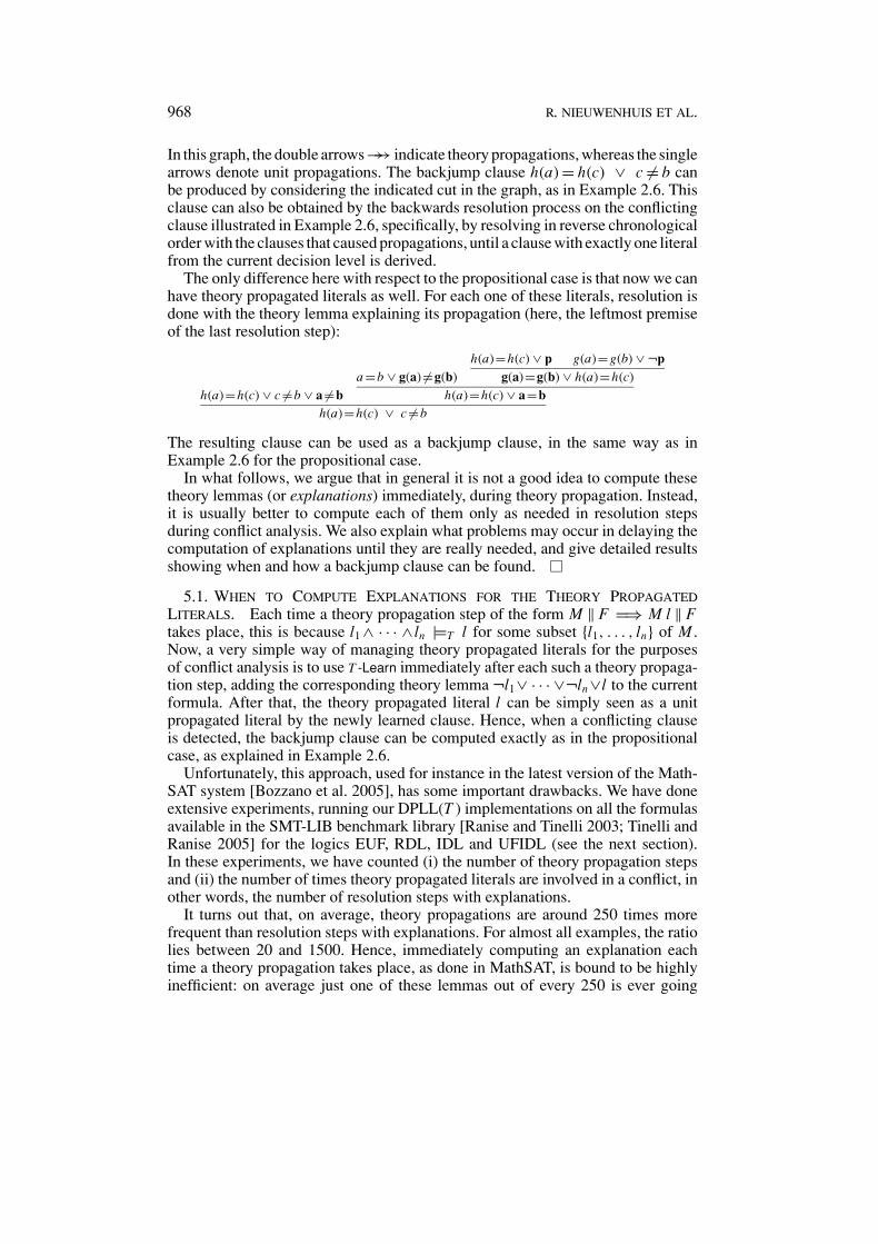
968 R. NIEUWENHUIS ET AL.
In this graph, the double arrows→→ indicate theory propagations, whereas the singlearrows denote unit propagations. The backjump clause h(a) = h(c) ∨ c �= b canbe produced by considering the indicated cut in the graph, as in Example 2.6. Thisclause can also be obtained by the backwards resolution process on the conflictingclause illustrated in Example 2.6, specifically, by resolving in reverse chronologicalorder with the clauses that caused propagations, until a clause with exactly one literalfrom the current decision level is derived.
The only difference here with respect to the propositional case is that now we canhave theory propagated literals as well. For each one of these literals, resolution isdone with the theory lemma explaining its propagation (here, the leftmost premiseof the last resolution step):
h(a)=h(c) ∨ c �=b ∨ a �=b
a =b ∨ g(a) �=g(b)h(a)=h(c) ∨ p g(a)=g(b) ∨ ¬p
g(a)=g(b) ∨ h(a)=h(c)h(a)=h(c) ∨ a=b
h(a)=h(c) ∨ c �=b
The resulting clause can be used as a backjump clause, in the same way as inExample 2.6 for the propositional case.
In what follows, we argue that in general it is not a good idea to compute thesetheory lemmas (or explanations) immediately, during theory propagation. Instead,it is usually better to compute each of them only as needed in resolution stepsduring conflict analysis. We also explain what problems may occur in delaying thecomputation of explanations until they are really needed, and give detailed resultsshowing when and how a backjump clause can be found.
5.1. WHEN TO COMPUTE EXPLANATIONS FOR THE THEORY PROPAGATEDLITERALS. Each time a theory propagation step of the form M ‖ F =⇒ M l ‖ Ftakes place, this is because l1 ∧ · · · ∧ln |=T l for some subset {l1, . . . , ln} of M .Now, a very simple way of managing theory propagated literals for the purposesof conflict analysis is to use T -Learn immediately after each such a theory propaga-tion step, adding the corresponding theory lemma ¬l1∨ · · · ∨¬ln ∨l to the currentformula. After that, the theory propagated literal l can be simply seen as a unitpropagated literal by the newly learned clause. Hence, when a conflicting clauseis detected, the backjump clause can be computed exactly as in the propositionalcase, as explained in Example 2.6.
Unfortunately, this approach, used for instance in the latest version of the Math-SAT system [Bozzano et al. 2005], has some important drawbacks. We have doneextensive experiments, running our DPLL(T ) implementations on all the formulasavailable in the SMT-LIB benchmark library [Ranise and Tinelli 2003; Tinelli andRanise 2005] for the logics EUF, RDL, IDL and UFIDL (see the next section).In these experiments, we have counted (i) the number of theory propagation stepsand (ii) the number of times theory propagated literals are involved in a conflict, inother words, the number of resolution steps with explanations.
It turns out that, on average, theory propagations are around 250 times morefrequent than resolution steps with explanations. For almost all examples, the ratiolies between 20 and 1500. Hence, immediately computing an explanation eachtime a theory propagation takes place, as done in MathSAT, is bound to be highlyinefficient: on average just one of these lemmas out of every 250 is ever going

Solving SAT and SAT Modulo Theories 969
to be used (possibly, even less than that, as each theory propagated literal mayoccur in more than one conflict). The cost of generating explanations is twofold:it is the cost incurred by SolverT in computing the clause and that incurred byDPLL(X ) in inserting the clause in the clause database and maintaining it underpropagation.
There is however a potential advantage in the MathSAT approach, for strategieswhere TheoryPropagate is applied only if no other rule except Decide is applicable(this is what we did for EUF in Section 4.4). Assume as before that TheoryPropagateapplies to a state M ‖ F because l1∧ · · · ∧ln |=T l for for some subset {l1, . . . , ln}of M . Also assume that, due to a previous TheoryPropagate step, the explanation¬l1∨ · · · ∨¬ln ∨ l is still present in F , although, due to backtracking, l has becomeagain undefined in M . Then the effect of theory propagating l can now be achievedmore efficiently by a unit propagation step with the clause ¬l1∨· · ·∨¬ln ∨ l. If thisleads to a conflict at the current decision level before TheoryPropagate is tried, thena gain in efficiency may be obtained. If, on the other hand, no conflict occurs beforeapplying TheoryPropagate, then it is likely that repeated work is done by SolverT ,rediscovering the fact that l is a T -consequence of M .
For some theory solvers, it may be possible that, when computing a T -consequence, there is only a low additional cost in computing its explanation aswell at the same time. But even then one usually would not want to pay the timeand memory cost of adding the lemma as a new clause—since in many cases this isgoing to be wasted work and space. One could simply store the lemma as a passiveclause, that is, not active in the DPLL procedure, or store some information on howto compute it later.
5.2. HANDLING CONFLICT ANALYSIS IN THE CONTEXT OF THEORYPROPAGATION. In the previous subsection we have argued that it is preferableto generate explanations only at the moment they are needed for conflict analysis.Here we analyze the possible problems that arise in doing so, and discuss whenand how it is still possible to compute a backjump clause. In a state of the formM1 l M2 l ′ M3 ‖ F , we say that l is older than l ′, and that l ′ is newer than l.
Too new explanations:Let us first revisit Example 5.1. After the four steps, where Clause 3 is conflicting, ifSolverT is asked to compute the explanation of a �=b, it can also return g(a) �=g(b),instead of the “real” explanation h(a) = h(c) ∨ c �= b ∨ a �= b. Indeed a �= b is aT -consequence of g(a) �= g(b) as well. But g(a) �= g(b) is a too new explanation:it did not even belong to the partial assignment at the time a �= b was propagated,and was in fact deduced by UnitPropagate from a �= b itself and Clause 1. Toonew explanations are problematic because they can cause cycles in the conflictgraph:

970 R. NIEUWENHUIS ET AL.
For the conflict graph above, the backwards resolution process computing the back-jump clause does in fact loop:
g(a)=g(b) ∨ a �=b
a =b ∨ g(a) �=g(b)h(a)=h(c) ∨ p g(a)=g(b) ∨ ¬p
g(a)=g(b) ∨ h(a)=h(c)h(a)=h(c) ∨ a=b
g(a)=g(b) ∨ h(a)=h(c)
Therefore, to make sure that a backjump clause can be found, SolverT should neverreturn too new explanations. A sufficient condition is to require that all literals inthe explanation of a literal l be older than l. In other words, if the current state is ofthe form M l N ‖ F , then all literals in the explanation of l should occur in M .
Too old explanations:In our example, when SolverT was asked to compute the explanation of a �= b, itcould also have returned f (a) �= f (b). This literal was already available beforea �=b was obtained, but, as mentioned in Section 4.4, SolverT might have failed todetect a �= b as a negative consequence of it. It is interesting to observe that, withf (a) = f (b) ∨ a �= b as the explanation of a �= b, the resulting conflict graph hasno unique implication point (UIP). In fact, there is not even a path from the currentdecision literal h(a) �= h(c) to the conflicting literal (of the current decision level)g(a) �=g(b):
However, looking at what happens with the backwards resolution procedure, onecan see that it still produces a backjump clause, that is, a clause with exactly oneliteral from the current decision level:
f (a)= f (b) ∨ a �=b
a =b ∨ g(a) �=g(b)h(a)=h(c) ∨ p g(a)=g(b) ∨ ¬p
g(a)=g(b) ∨ h(a)=h(c)h(a)=h(c) ∨ a=b
h(a)=h(c) ∨ f (a)= f (b)
The following theorem states that in the backwards resolution process too old ex-planations are never a problem. It follows that just disallowing too new explanationssuffices to guarantee that a backjump clause is always found.
THEOREM 5.2. Assume that for any state of the form M ‖ F and for any l inM due to TheoryPropagate, the explanation of l produced by SolverT contains noliterals newer than l in M. Then, if some clause C is conflicting in a state S, eitherFail applies to S, or else the backwards resolution process applied to C reaches abackjump clause.
PROOF. Let d be the largest of the decision levels of the literals in C , and let Dbe the (nonempty) set of all literals of C that have become false at decision leveld . If D is a singleton, C itself is a backjump clause. Otherwise, we can apply the

Solving SAT and SAT Modulo Theories 971
backwards conflict resolution process, resolving away literals of decision level d,until we reach a backjump clause having exactly one literal of level d. This processalways terminates because each resolution step replaces a literal of decision leveld by a finite number (zero in the case of a too old explanation) of strictly olderliterals of level d. The process is also guaranteed to produce a clause with just oneliteral of decision level d because, except for the decision literal itself, every literalof decision level d is resolvable.
Note that the previous theorem is rather general by making no assumptionson the strategy followed in applying the DPLL rules. Also note that the theoremholds in the purely propositional case a well, where the theory T is empty andthe theorem’s assumption is vacuously true as TheoryPropagate never applies. Itsgenerality entails that, for instance, one can apply Decide even in the presence of aconflicting clause, or if UnitPropagate also applies. In contrast, in Zhang and Malik[2003], the correctness proof of the Chaff algorithm assumes the fixed standardstrategy in which unit propagation is done exhaustively before making any newdecisions, which is considered an “important invariant”. Theorem 5.2 instead showsthat it is unproblematic for conflict analysis if a literal l is unit propagated at adecision level d when in fact it could have been propagated already at an earlierlevel. The reason is simply that in the backwards resolution step resolving on lreplaces it by zero literals of level d, in perfect analogy to what happens to theorypropagated literals with a too old explanation.
5.3. THE DEGREE OF EAGERNESS BY WHICH THEORY PROPAGATION SHOULD BEPERFORMED. So far, we have seen two possible strategies for theory propagation.
The first one, which we defined for Difference Logic, requires that SolverT returnsall theory consequences (Section 4.2). In that strategy, TheoryPropagate is invokedeach time a new literal is added to the current partial assignment. This is done toensure that the partial assignment never becomes T -inconsistent.
The second strategy, defined for EUF logic, assumes that SolverT may return onlysome subset of the theory consequences, and applies TheoryPropagate only if no ruleother than TheoryPropagate or Decide is applicable (Section 4.4).
However, there may also be expensive theories where one does not want to do fulltheory propagation (or check T -consistency) before every Decide step, but insteadinvoke it in some cheaper, incomplete way. The complete check is only requiredat the leaves of the search tree, that is, each time a propositional model has beenfound, in order to decide its T -consistency (this coincides with what is done in thenaive lazy approach). The MathSAT approach [Bozzano et al. 2005] is based on asimilar hierarchical view, where cheaper checks are performed more eagerly thanexpensive ones.
6. Experiments with an Implementation of DPLL(T )
We have experimented the DPLL(T ) architecture with various implementationscollaboratively developed in Barcelona and Iowa. We describe here our most ad-vanced implementation, Barcelogic, developed mostly in Barcelona. The systemfollows the strategies presented in Section 4, and its solvers are as described inSection 4.3 and in Nieuwenhuis and Oliveras [2003, 2005b]. Its DPLL(X ) engineimplements state-of-the-art techniques such as the two-watched literal scheme forunit propagation, the first-UIP learning scheme, and VSIDS-like decision heuristics

972 R. NIEUWENHUIS ET AL.
[Moskewicz et al. 2001; Zhang et al. 2001]. The T -Forget rule is currently appliedby DPLL(X ) after each restart, removing a portion of the learned clauses accordingto their activity level [Goldberg and Novikov 2002], defined as the number of timesthey were involved in a conflict since the last restart.
6.1. THE 2005 SMT COMPETITION. The effectiveness of Barcelogic was shownat the 2005 SMT Competition [Barrett et al. 2005]. The competition used problemsfrom the SMT-LIB library [Tinelli and Ranise 2005], a fairly large collection ofbenchmarks (around 1300) coming from such diverse areas as software and hard-ware verification, bounded model checking, finite model finding, and scheduling.These benchmarks were in the standard format of SMT-LIB [Ranise and Tinelli2003], and were classified into 7 competition divisions according to their back-ground theory and some additional syntactic restrictions. For each division, around50 benchmarks were randomly chosen and given to each entrant system with a timelimit of 10 minutes per benchmark.
Barcelogic entered and won all four divisions for which it had a theory solver:EUF, IDL and RDL (respectively, integer and real Difference Logic), and UFIDL(combining EUF and IDL). At least 10 systems participated in each of these divi-sions. Among the competitors were well-known SMT solvers such as SVC [Barrettet al. 1996], CVC [Barrett et al. 2002], CVC-Lite [Barrett and Berezin 2004], Math-SAT [Bozzano et al. 2005], and two very recent successors of ICS [Filliatre et al.2001]: Yices (by Leonardo de Moura) and Simplics (by Dutertre and de Moura).Apart from EUF and Difference Logic, these systems also support other theoriessuch as arrays (except MathSAT), and linear arithmetic (SVC only over the reals).
It is well-known that in practical problems over richer (combined) theories usu-ally a large percentage of the work still goes into EUF and Difference Logic. Forexample, in [Bozzano et al. 2005] it is mentioned that in many calls a general solveris not needed: “very often, the unsatisfiability can be established in less expressive,but much easier, sub-theories”. Similarly, Seshia and Bryant [2004], which dealswith quantifier-free Presburger arithmetic, states that it has been found by them andothers that literals are “mainly” difference logic.
The competition was run on 2.6 GHz, 512 MB, Pentium 4 Linux machines, witha 512 KB cache. For each division, the results of the best three systems are shownin the following table, where Total time is the total time in seconds spent by eachsystem, with a timeout of 600 seconds, and Time solved is the time spent on thesolved problems only:
# problems Total Time
Top-3 systems solved time solved
Barcelogic 39 8358 1758EUF (50 problems): Yices 37 9601 1801
MathSAT 33 12386 2186Barcelogic 41 6341 940
RDL (50 pbms.): Yices 37 9668 1868MathSAT 37 10408 2608Barcelogic 47 3531 1131
IDL (51 pbms.): Yices 47 4283 1883MathSAT 46 4295 1295Barcelogic 45 2705 305
UFIDL (49 pbms.): Yices 36 9789 1989MathSAT 22 17255 1055

Solving SAT and SAT Modulo Theories 973
Not only did Barcelogic solve more problems than each of the other systems, italso did so in considerably less time, even—and in spite of the fact that it solvedmore problems—if only the time spent on the solved problems is counted.
6.2. EXPERIMENTS ON THE IMPACT OF THEORY PROPAGATION. In our experi-ence, the overhead produced by theory propagation is almost always compensatedby a significant reduction of the search space. In Ganzinger et al. [2004] we pre-sented extensive experimental results showing its effectiveness in our DPLL(T )approach for EUF logic. In Nieuwenhuis and Oliveras [2005a] we discussed alarge number of experiments for Difference Logic, with additional emphasis onthe good scaling properties of the approach. The new SMT solver Yices now alsoheavily relies on theory propagation.
Of course, theory propagation may not pay off in certain specific problems wherethe theory plays an insignificant role, that is, where reasoning is done almost entirelyat the Boolean level. Such situations can be detected on the fly by computing thepercentage of conflicts caused by theory propagations. If this number is very low,theory propagation can be switched off automatically, or applied more lazily, tospeed up the computation. (This is done in a forthcoming release of our system.)
In the following two figures, Barcelogic with and without theory propagation iscompared, on the same type of machine as in the previous subsection, in terms ofrun time (in seconds) and number of decisions (applications of Decide) on a typicalreal-world Difference Logic suite (fisher6-mutex, see Tinelli and Ranise [2005]),consisting of 20 problems of increasing size.
The figures show the typical behavior on the larger problems where the theoryplays a significant role: both the run time and the number of decisions are ordersof magnitude smaller in the version with theory propagation (note that times anddecisions are plotted on a logarithmic scale). In both cases, the DPLL(X ) engineused was exactly the same, although in the exhaustive theory case some parts ofthe code were never executed (e.g., theory lemma learning).
6.3. EXPERIMENTS COMPARING BARCELOGIC WITH THE EAGER APPROACH.For completeness, we finally compare Barcelogic with UCLID, the best-known toolimplementing the eager translation approach to SMT [Lahiri and Seshia 2004]. Weshow below run time results (in seconds) for three typical series of benchmarks forUFIDL coming from different methods for pipelined processor verification givenin [Manolios and Srinivasan 2005a, 2005b] (more precisely, for the BIDW case (i)flushing, (ii) commitment good MA and (iii) commitment GFP). The benchmarks

974 R. NIEUWENHUIS ET AL.
were run on the same type of machine as in the previous two subsections, but thistime with a one hour timeout. We used Siege [Ryan 2004] as the final SAT solverfor UCLID, since it performed better than any other available SAT solver on theseproblems.
6-stage:7-stage:8-stage:9-stage:
10-stage:
UCLID BLogic
258 1835 33160 15
>3600 23>3600 54
UCLID BLogic
3596 5>3600 8>3600 18>3600 18>3600 29
UCLID BLogic
19 158 1
226 1664 1
>3600 2
We emphasize that these results are typical for the pipelined processor verificationproblems coming from this source, a finding that has also independently beenreproduced by P. Manolios (private communication). We refer the reader to theresults given in Ganzinger et al. [2004], showing that our approach also dominatesUCLID in the pure EUF case, as well as for EUF with integer offsets (interpretedsuccessor and predecessor symbols).
7. Conclusions
We have shown that the Abstract DPLL formalism introduced here can be veryuseful for understanding and formally reasoning about a large variety of DPLL-based procedures for SAT and SMT.
In particular, we have used it here to describe several variants of a new, effi-cient, and modular approach for SMT, called DPLL(T ). Given a DPLL(X ) en-gine, a DPLL(T ) system for a theory T is obtained by simply plugging in thecorresponding theory solver SolverT , which must only be able to deal with con-junctions of theory literals and conform to a minimal and simple set of additionalrequirements.
We are currently working on several—in our opinion very promising—ways toimprove and extend both the abstract framework and the DPLL(T ) architecture.
The abstract framework can be extended to deal more effectively with theorieswhere the satisfiability of conjunctions of literals is already NP-hard by lifting, fromthe theory solver to the DPLL(X ) engine, some or all of the case analysis done bythe theory solver. Along those lines, the framework can also be nicely extendedto a Nelson-Oppen style combination framework for handling formulas over sev-eral theories. The resulting DPLL(T1, . . . , Tn) architecture can deal modularly andefficiently with the combined theories.
Preliminary experiments reveal that other applications of the DPLL(T ) frame-work can produce competitive decision procedures as well for completely different(at least on the surface) kinds of problems. For example, optimization aspects ofproblems such as pseudo-Boolean constraints can be nicely expressed and effi-ciently solved in this framework by recasting them as particular SMT problems.
ACKNOWLEDGMENTS. We would like to thank Roberto Sebastiani for a number ofinsightful discussions and comments on the lazy SMT approach and DPLL(T ).We are also grateful to the anonymous referees for their helpful suggestions onimproving this article.

Solving SAT and SAT Modulo Theories 975
REFERENCES
ALUR, R. 1999. Timed automata. In Proceedings of the 11th International Conference on ComputerAided Verification (CAV’99) (Trento, Italy), N. Halbwachs and D. Peled, Eds. Lecture Notes in ComputerScience, vol. 1633. Springer-Verlag, New York, 8–22.
ARMANDO, A., CASTELLINI, C., AND GIUNCHIGLIA, E. 2000. SAT-based procedures for temporal reason-ing. In Proceedings of the 5th European Conference on Planning (Durham, UK), S. Biundo and M. Fox,Eds. Lecture Notes in Computer Science, vol. 1809. Springer-Verlag, New York, 97–108.
ARMANDO, A., CASTELLINI, C., GIUNCHIGLIA, E., AND MARATEA, M. 2004. A SAT-based decisionprocedure for the Boolean combination of difference constraints. In Proceedings of the 7th InternationalConference on Theory and Applications of Satisfiability Testing (SAT 2004). Lecture Notes in ComputerScience. Springer-Verlag, New York.
AUDEMARD, G., BERTOLI, P., CIMATTI, A., KORNILOWICZ, A., AND SEBASTIANI, R. 2002. A SAT basedapproach for solving formulas over Boolean and linear mathematical propositions. In Proceedings of theCADE-18. Lecture Notes in Computer Science, vol. 2392. Springer-Verlag, New York, 195–210.
BALL, T., COOK, B., LAHIRI, S. K., AND ZHANG, L. 2004. Zapato: Automatic theorem proving forpredicate abstraction refinement. In Proceedings of the 16th International Conference on ComputerAided Verification (CAV’04) (Boston, MA). R. Alur and D. Peled, Eds. Lecture Notes in ComputerScience, vol. 3114. Springer-Verlag, New York. 457–461.
BARRETT, C., DE MOURA, L., AND STUMP, A. 2005. SMT-COMP: Satisfiability modulo theories compe-tition. In Proceedings of the 17th International Conference on Computer Aided Verification, K. Etessamiand S. Rajamani, Eds. Lecture Notes in Computer Science, vol. 3576. Springer-Verlag, New York, 20–23.(See www.csl.sri.com/users/demoura/smt-comp.)
BARRETT, C., DILL, D., AND STUMP, A. 2002. Checking satisfiability of first-order formulas by incre-mental translation into SAT. In Proceedings of the 14th International Conference on Computer AidedVerification (CAV). Lecture Notes in Computer Science, vol. 2404. Springer-Verlag, New York.
BARRETT, C., DILL, D. L., AND LEVITT, J. 1996. Validity checking for combinations of theories withequality. In Proceedings of the 1st International Conference on Formal Methods in Computer AidedDesign. Lecture Notes in Computer Science, vol. 1166. Springer-Verlag, New York, 187–201.
BARRETT, C. W. 2003. Checking validity of quantifier-free formulas in combinations of first-order the-ories. Ph.D. dissertation. Stanford University, Stanford, CA.
BARRETT, C. W., AND BEREZIN, S. 2004. CVC lite: A new implementation of the cooperating validitychecker. In Proceedings of the 16th International Conference on Computer Aided Verification (CAV’04)(Boston, MA). R. Alur and D. Peled, Eds. Lecture Notes in Computer Science, vol. 3114. Springer-Verlag,New York, 515–518.
BAYARDO, R. J. J., AND SCHRAG, R. C. 1997. Using CSP look-back techniques to solve real-worldSAT instances. In Proceedings of the 14th National Conference on Artificial Intelligence (AAAI’97)(Providence, RI), 203–208.
BEAME, P., KAUTZ, H., AND SABHARWAL, A. 2003. On the power of clause learning. In Proceedings ofIJCAI-03, 18th International Joint Conference on Artificial Intelligence (Acapulco, MX).
BONET, M. L., ESTEBAN, J. L., GALESI, N., AND JOHANNSEN, J. 2000. On the relative complexity ofresolution refinements and cutting planes proof systems. SIAM J. Comput. 30, 5, 1462–1484.
BOZZANO, M., BRUTTOMESSO, R., CIMATTI, A., JUNTTILA, T. V. ROSSUM, P., SCHULZ, S., AND SEBASTIANI,R. 2005. An incremental and layered procedure for the satisfiability of linear arithmetic logic. In Toolsand Algorithms for the Construction and Analysis of Systems, 11th International Conference (TACAS).Lecture Notes in Computer Science, vol. 3440. Springer-Verlag, New York, 317–333.
BRYANT, R., GERMAN, S., AND VELEV, M. 2001. Processor verification using efficient reductions of thelogic of uninterpreted functions to propositional logic. ACM Trans. Computational Logic 2, 1, 93–134.
BRYANT, R., LAHIRI, S., AND SESHIA, S. 2002. Modeling and verifying systems using a logic of counterarithmetic with lambda expressions and uninterpreted functions. In Proceedings of the 14th InternationalConference on Computer Aided Verification (CAV). Lecture Notes in Computer Science, vol. 2404.Springer-Verlag, New York.
BRYANT, R. E., AND VELEV, M. N. 2002. Boolean satisfiability with transitivity constraints. ACM Trans.Computational Logic 3, 4, 604–627.
BURCH, J. R., AND DILL, D. L. 1994. Automatic verification of pipelined microprocessor control. InProceedings of the 6th International Conference on Computer Aided Verification (CAV). Lecture Notesin Computer Science, vol. 818. Springer-Verlag, New York. 68–80.
DAVIS, M., LOGEMANN, G., AND LOVELAND, D. 1962. A machine program for theorem-proving. Com-mun. ACM 5, 7, 394–397.

976 R. NIEUWENHUIS ET AL.
DAVIS, M., AND PUTNAM, H. 1960. A computing procedure for quantification theory. J ACM 7, 201–215.DE MOURA, L., AND RUEß, H. 2002. Lemmas on demand for satisfiability solvers. In Proceedings of the
5th International Symposium on the Theory and Applications of Satisfiability Testing (SAT’02). 244–251.DE MOURA, L., AND RUESS, H. 2004. An experimental evaluation of ground decision procedures. In
Proceedings of the 16th International Conference on Computer Aided Verification (CAV’04) (Boston,MA). R. Alur and D. Peled, Eds. Lecture Notes in Computer Science, vol. 3114. Springer-Verlag, NewYork, 162–174.
DE MOURA, L., RUEß, H., AND SHANKAR, N. 2004. Justifying equality. In Proceedings of the 2ndWorkshop on Pragmatics of Decision Procedures in Automated Reasoning (Cork, Ireland).
DOWNEY, P. J., SETHI, R., AND TARJAN, R. E. 1980. Variations on the common subexpressions problem.J. ACM 27, 4, 758–771.
EEN, N., AND SORENSSON, N. 2003. An extensible SAT-solver. In Proceedings of the 6th InternationalConference on Theory and Applications of Satisfiability Testing (SAT). 502–518.
FILLIATRE, J.-C., OWRE, S., RUEß, H., AND SHANKAR, N. 2001. ICS: Integrated canonization and solving(tool presentation). In Proceedings of the 13th International Conference on Computer Aided Verification(CAV’2001). G. Berry, H. Comon, and A. Finkel, Eds. Lecture Notes in Computer Science, vol. 2102.Springer-Verlag, New York, 246–249.
FLANAGAN, C., JOSHI, R., OU, X., AND SAXE, J. B. 2003. Theorem proving using lazy proof explanation.In Proceedings of the 15th International Conference on Computer Aided Verification (CAV). Lecture Notesin Computer Science, vol. 2725. Springer-Verlag, New York.
GANZINGER, H., HAGEN, G., NIEUWENHUIS, R., OLIVERAS, A., AND TINELLI, C. 2004. DPLL(T): FastDecision Procedures. In Proceedings of the 16th International Conference on Computer Aided Verification(CAV’04) (Boston, MA). R. Alur and D. Peled, Eds. Lecture Notes in Computer Science, vol. 3114.Springer-Verlag, New York, 175–188.
GOLDBERG, E., AND NOVIKOV, Y. 2002. BerkMin: A fast and robust SAT-solver. In Proceedings of theSymposium on Design, Automation, and Test in Europe (DATE ’02). 142–149.
HODGES, W. 1993. Model Theory. Enclyclopedia of mathematics and its applications, vol. 42. CambridgeUniversity Press, Cambridge, MA.
JAFFAR, J., AND MAHER, M. 1994. Constraint Logic Programming: A Survey. J. Logic Prog. 19/20,503–581.
LAHIRI, S. K., AND SESHIA, S. A. 2004. The UCLID Decision Procedure. In Computer Aided Verification,16th International Conference (CAV). Lecture Notes in Computer Science, vol. 3114. Springer-Verlag,New York, 475–478.
MANOLIOS, P., AND SRINIVASAN, S. K. 2005a. A computationally efficient method based on commit-ment refinement maps for verifying pipelined machines. In Proceedings of the ACM IEEE InternationalConference on Formal Methods and Models for Co-Design (MEMOCODE). ACM, New York.
MANOLIOS, P., AND SRINIVASAN, S. K. 2005b. Refinement maps for efficient verification of processormodels. In Proceedings of the Design, Automation and Test in Europe Conference and Exposition (DATE).IEEE Computer Society, 1304–1309.
MARQUES-SILVA, J., AND SAKALLAH, K. A. 1999. GRASP: A search algorithm for propositional satis-fiability. IEEE Trans. Comput. 48, 5 (May), 506–521.
MEIR, O., AND STRICHMAN, O. 2005. Yet another decision procedure for equality logic. In Proceedingsof the 17th International Conference on Computer Aided Verification (CAV’05) (Edimburgh, Scotland).K. Etessami and S. K. Rajamani, Eds. Lecture Notes in Computer Science, vol. 3576. Springer-Verlag,New York, 307–320.
MOSKEWICZ, M. W., MADIGAN, C. F., ZHAO, Y., ZHANG, L., AND MALIK, S. 2001. Chaff: Engineeringan efficient SAT solver. In Proceedings of the 38th Design Automation Conference (DAC’01).
NIEUWENHUIS, R., AND OLIVERAS, A. 2003. Congruence Closure with Integer Offsets. In Proceedingsof the 10h International Conference on Logic for Programming, Artificial Intelligence and Reasoning(LPAR), M. Vardi and A. Voronkov, Eds. Lecture Notes in Artificial Intellegence, vol. 2850. Springer-Verlag, New York, 2850. 78–90.
NIEUWENHUIS, R., AND OLIVERAS, A. 2005a. DPLL(T) with exhaustive theory propagation and itsapplication to difference logic. In Proceedings of the 17th International Conference on Computer AidedVerification (CAV’05) (Edimburgh, Scotland). K. Etessami and S. K. Rajamani, Eds. Lecture Notes inComputer Science, vol. 3576. Springer-Verlag, New York, 321–334.
NIEUWENHUIS, R., AND OLIVERAS, A. 2005b. Proof-producing congruence closure. In Proceedings ofthe 16th International Conference on Term Rewriting and Applications (RTA’05) (Nara, Japan). J. Giesl,Ed. Lecture Notes in Computer Science, vol. 3467. Springer-Verlag, New York, 453–468.

Solving SAT and SAT Modulo Theories 977
NIEUWENHUIS, R., OLIVERAS, A., AND TINELLI, C. 2005. Abstract DPLL and abstract DPLL modulotheories. In Proceedings of the 11th International Conference Logic for Programming, Artificial Intel-ligence and Reasoning (LPAR). F. Baader and A. Voronkov, Eds. Lecture Notes in Computer Science,vol. 3452. Springer-Verlag, New York, 36–50.
PNUELI, A., RODEH, Y., SHTRICHMAN, O., AND SIEGEL, M. 1999. Deciding equality formulas by smalldomains instantiations. In Proceedings of the 11th International Conference on Computer Aided Verifi-cation (CAV). Lecture Notes in Computer Science, vol. 1633. Springer-Verlag, New York. 455–469.
RANISE, S., AND TINELLI, C. 2003. The SMT-LIB format: An initial proposal. In Proceedings of the 1stWorkshop on Pragmatics of Decision Procedures in Automated Reasoning. Miami.
RYAN, L. 2004. Efficient algorithms for clause-learning SAT solvers. M.S. dissertation, School of Com-puting Science, Simon Fraser University.
SCHRIJVER, A. 1987. Theory of Linear and Integer Programming. Wiley, New York.SESHIA, S., LAHIRI, S., AND BRYANT, R. 2003. A hybrid SAT-based decision procedure for separation
logic with uninterpreted functions. In Proceedings of the 40th Design Automation Conference (DAC).425–430.
SESHIA, S. A. 2005. Adaptive eager Boolean encoding for arithmetic reasoning in verification. Ph.D.dissertation, Carnegie-Mellon University, Pittsburgh, PA.
SESHIA, S. A., AND BRYANT, R. E. 2004. Deciding quantifier-free presburger formulas using parameter-ized solution bounds. In Proceedings of the 19th IEEE Symposium on Logic in Computer Science (LICS2004). IEEE Computer Society Press, Los Alamitos, CA, 100–109.
STRICHMAN, O. 2002. On solving presburger and linear arithmetic with SAT. In Proceedings of theFormal Methods in Computer-Aided Design, 4th International Conference (FMCAD 2002) (Portland,OR). M. Aagaard and J. W. O’Leary, Eds. Lecture Notes in Computer Science, vol. 2517. Springer-Verlag,New York, 160–170.
STRICHMAN, O., SESHIA, S. A., AND BRYANT, R. E. 2002. Deciding separation formulas with SAT. InProceedings of the 14th International Conference on Computer Aided Verification (CAV). Lecture Notesin Computer Science, vol 2404. Springer-Verlag, New York. 209–222.
STUMP, A., AND TAN, L.-Y. 2005. The algebra of equality proofs. In Proceedings of the 16th InternationalConference on Term Rewriting and Applications, RTA’05 (Nara, Japan). J. Giesl, Ed. Lecture Notes inComputer Science, vol. 3467. Springer-Verlag, New York, 469–483.
TALUPUR, M., SINHA, N., STRICHMAN, O., AND PNUELI, A. 2004. Range allocation for separation logic. InProceedings of the 16th International Conference on Computer Aided Verification (CAV 2004). (Boston,MA July 13–17). Lecture Notes in Computer Science, Springer-Verlag, New York, 148–161.
TINELLI, C. 2002. A DPLL-based calculus for ground satisfiability modulo theories. In Proceedings ofthe 8th European Conference on Logics in Artificial Intelligence. Lecture Notes in Artificial Intelligence,vol. 2424. Springer-Verlag, New York, 308–319.
TINELLI, C., AND RANISE, S. 2005. SMT-LIB: The Satisfiability Modulo Theories Library.http://goedel.cs.uiowa.edu/smtlib/.
ZHANG, H. 1997. SATO: An efficient propositional prover. In Proceedings of the 14th InternationalConference on Automated Deduction. Springer-Verlag, New York, 272–275.
ZHANG, L., MADIGAN, C. F., MOSKEWICZ, M. W., AND MALIK, S. 2001. Efficient conflict driven learningin a Boolean satisfiability solver. In Proceedings of the International Conference on Computer-AidedDesign (ICCAD’01). 279–285.
ZHANG, L., AND MALIK, S. 2003. Validating SAT solvers using an independent resolution-based checker:Practical implementations and other applications. In Proceedings of the 2003 Design, Automation and Testin Europe Conference (DATE 2003). IEEE Computer Society Press, Los Alamitos, CA, 10880–10885.
RECEIVED DECEMBER 2005; REVISED FEBRUARY 2006 AND JULY 2006; ACCEPTED NOVEMBER 2006
Journal of the ACM, Vol. 53, No. 6, November 2006.