Solving the Travelling Salesman Problem

with a Hopfield - type neural network

Jacek Mandziuk

Institute of Mathematics, Warsaw University of Technology,

Plac Politechniki 1, 00-661 Warszawa, Poland.

Abstract

In this paper a modification of the Hopfield neural network solving the Travelling Salesman

Problem (TSP) is proposed. Two strategies employed to achieve the solution and results of the

computer simulations are presented.

The network exhibits good performance in escaping from local minima of the energy surface of

the problem. With a judicious choice of network internal parameters nearly 100% convergence to

valid tours is achieved.

Extensive simulations indicate that the quality of results is independent on the initial state of

the network.

Key Words : neural network, NP-Hard optimization problem, Travelling Sales-

man Problem, Hopfield network, N-Queens Problem

e-mail : mandziuk@alpha.im.pw.edu.pl

tel./fax : (48 22) 621 93 12

Published in Demonstratio Mathematica, 29(1), 219-231, (1996)

1

1 INTRODUCTION

Hopfield-type neural networks (Hopfield 1984) composed of highly-interconnected

analog elements (neurons) can be successfully used in solving optimization problems.

Structure of a network and weights of connections between neurons depend on the

specific constraints of a problem. For each neuron in the network the so-called input

and output potentials can be defined, denoted by u and v, respectively. In the

Hopfield model, the function of response is usually S-shaped. In this paper

v(u) = 1/2 [1 + tanh(αu)] (1)

where α is a gain of that function. For sufficiently big values of α, v is of binary

character, i.e. approximately

v(u) ={ 0 if u < 0

1 if u > 0

In a network composed of m neurons a function of energy E of the network is in

general of the following form (Hopfield 1984; Hopfield and Tank 1985):

E = −12

m∑

i=1

m∑

j=1

tijvivj (2)

where tij (i, j = 1, . . . , m) is weight of a connection between the output of the j − th

neuron and the input of the i− th one. All tij form a matrix of connection weights.

They can be positive (excitatory stimulus) or negative (inhibitory stimulus) or equal

to zero, i.e. there is no connection from neuron j to neuron i. The input potential

ui of the i− th neuron is defined by the equation

ui = −∂E

∂vi(i = 1, . . . , m) (3)

From (2) and (3) we obtain

ui =m∑

j=1

tijvj (i = 1, . . . , m) (4)

2

The above rules were exploit by various authors in attempts to solve hard opti-

mization problems. The greatest attention among them was probably paid to the

TSP. The problem can informally be stated as follows:

Definition 1

Given the set of n cities and distances between every two of them, find the closed

tour for the salesman through all cities that visits each city only once and is of

minimum length.

Based on the Graph Theory terminology the TSP is defined as below:

Definition 2

Given a graph Kn and a symmetric matrix representing weights of edges in Kn,

find the Hamiltonian cycle in Kn of minimum length (cost).

Note 1

Problem definition presented here is not the only possible version of the TSP. In

other definitions, the matrix is not symmetric or not every two different cities are

connected by an edge. Some alternative definitions, as well as main, well known

theoretical results concerning the computational complexity of various versions of

the TSP can be found in the paper of Reingold et al. (1985).

Note 2

Since, the two above mentioned definitions are equivalent, and due to some ”tradi-

tion” associated with formulating the TSP is terms of ”route across cities”, we would

rather use terminology from Definition 1.

Due to the presumable non-polynomial complexity of the TSP, conventional ap-

proaches to solving the problem are based either on the extensive search methods or

on heuristics. The most popular and one of the best heuristical methods are those

presented in Lin and Kernighan (1973), Dantzig et al. (1954, 1959) or Padberg and

Rinaldi (1987).

Our solution to the problem is based on the papers of Yao et al. (1989), Mandziuk

and Macukow (1992), and Mandziuk (1993). Actually, the idea of network evolution

3

as well as the way of choosing starting point of the simulation are identical to the

ones used for the N-Queens Problem (NQP) in the last two of above cited papers.

The fact that these two problems are well suited to the method proposed is en-

couraging and stimulating for future research and development of the method.

In this paper, any syntactically valid solution of the TSP (Hamiltonian cycle in a

city graph) will be treated as solution of the problem, and solutions that minimize

length of the tour will be called best solutions. Obviously, for any solution there exist

2n−1 other solutions of the same length which differ from one another in the starting

city or direction of the tour. For the sake of simplicity, all of them would be treated

as the same solution.

Solving optimization problems with the Hopfield network requires careful and ade-

quate choice of the energy function, i.e. weights tij . Function E must be determined

in such a way that its minima correspond to solutions of the problem considered.

In this paper E is of the form

E = E1 + E2 (5)

where

E1 =A

2

n∑x=1

n∑

i=1

n∑

j=1j 6=i

vxivxj +B

2

n∑

i=1

n∑x=1

n∑y=1y 6=x

vxivyi +C

2(

n∑x=1

n∑

i=1

vxi − (n + σ))2 (5.1)

and

E2 =D

2

n∑x=1

n∑y=1y 6=x

n∑

i=1

dxyvxi(vy,i+1 + vy,i−1) (5.2)

In eqs. (5.1) and (5.2), n denotes the number of cities, and dxy the distance between

cities x and y.

The way of solving the TSP presented here, except for different choice of network

parameters, differs from the classical approach in the way of updating neurons output

4

potentials. Hopfield (1984) and others (Wilson and Pawley 1988; Kamgar-Parsi and

Kamgar-Parsi 1988; Bizzarri 1991) have used the following updating rule

duxi

dt= −uxi

τ−A

n∑

j=1j 6=i

vxj −B

n∑y=1y 6=x

vyi − C(n∑

x=1

n∑

j=1

vxj − (n + σ))−

D

n∑y=1

dxy(vy,i+1 + vy,i−1)

(6)

with τ = 1.

In the practical computer realization, after applying the Euler method, eq. (6) was

of the form

uxi(t + ∆t) =uxi(t) + ∆t(−uxi(t)−A

∑

j 6=i

vxj(t)−B∑

x 6=y

vyi(t)−

C(n∑

x=1

n∑

j=1

vxj(t)− (n + σ))−D

n∑y=1

dxy(vy,i+1(t) + vy,i−1(t))) (7)

with ∆t equal to 10−5.

In eq. (7) the state of neuron xi (x, i = 1, . . . , n) at time t + 1 depends on its

state at time t. In our simulations an input potential at time t + 1 does not directly

depend on its state in the previous moment. Actually, from (3) and (5)

uxi(t + 1) = −A

n∑

j=1j 6=i

vxj(t)−B

n∑y=1y 6=x

vyi(t)− C(n∑

x=1

n∑

j=1

vxj(t)− (n + σ))−

D

n∑y=1

dxy(vy,i+1(t) + vy,i−1(t))

(8)

The above presented updating rule was also used by Yao et al. (1989). The

authors reported about 50% convergence rate to valid tours. The better convergence

rate obtained in our simulations is due to the better choice of network constants.

The biggest advantage of the proposed network is its independence on the initial

state (the output potentials of neurons at the beginning of a simulation test). Results

of computer simulations as well as discussion of the influence of network constants

on the quality of results are presented in the following sections.

5

2 NETWORK DESCRIPTION AND SIMULATION RESULTS

In computer simulations the network was represented by a matrix Vn×n. At the end

of a simulation test which converged to a solution each element vxi (x, i = 1, . . . , n),

representing output potential of neuron xi, was equal to either zero or 1. Moreover,

elements of V fulfilled the constraints that in each row and in each column of V

there existed exactly one element equal to 1. In the resulting matrix, vxi = 1 was

interpreted as that city x was in the i - th position in a salesman’s tour.

The above requirements for resulting matrix V were implied by the condition that

minima of (5) should correspond to solutions of the problem.

Actually, in (5.1) term multiplied by A fulfils the constraint that in each row x

there exist at most one element equal to 1 (city x is visited not more than once).

Similarly, term multiplied by B fulfils the same condition for columns (at the i - th

step of the tour at most one city is visited). Finally, the third term in (5.1) forces the

sum of all elements of V to a value close to n, which means that the tour is composed

of n steps.

Minimization of a tour length is covered by (5.2).

In a simulation test, the network starting from some energy level, slowly decreases

its energy and, in the end, settles in the minimum of E. The ”deeper” the mini-

mum, the better the obtained solution (global minimum of E corresponds to the best

solution).

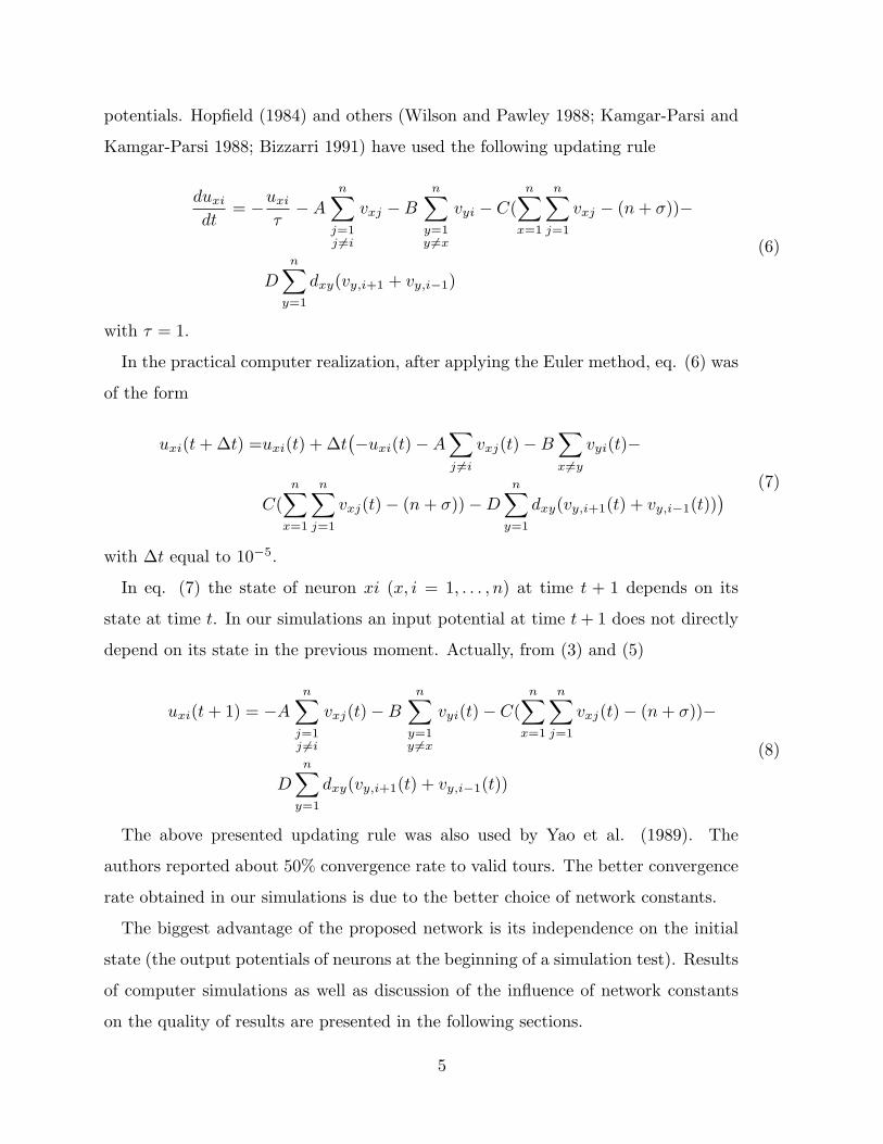
A single simulation test was performed as follows (see Fig. 1) :

(i) all initial output potentials vxi (x, i = 1, . . . , n) were set and from (5) the

starting value of energy E was evaluated,

(ii) neuron (x, i) was chosen at random and from (8) uxi was calculated, and then

from (1) vxi was obtained.

Operation (ii) was repeated 5n2 times, and then a new value of E from (5) was

calculated.

Every n2 repetitions of (ii) was called an internal iteration. Five internal iterations

composed one external iteration.

6

A simulation process terminated if the energy remained constant in a priori estab-

lished amount of successive external iterations or, the number of external iterations

exceeded the constraint for global number of iterations and the network still did not

achieve a stable state, i.e. a constant value of E.

In simulation tests four strategies for setting initial output potentials were used.

In those strategies the output of each of n2 neurons was initially set to (cf. Mandziuk

and Macukow 1992; Mandziuk 1993):

a - random value from [0, β],

b - random value from [0, 1],

c - random value from [1− β, 1],

d - random value from [0, β] + 1/n,

where β ≈ 0.03.

Two strategies, denoted F (Full) and P (Part) were employed for choosing neuron

xi to be modified in (ii).

In case F , the choice of neurons to be modified in the internal iteration was com-

pletely random. In case P , in every internal iteration a permutation of numbers

1, . . . , n2 was randomly chosen, and neurons were modified according to that permu-

tation.

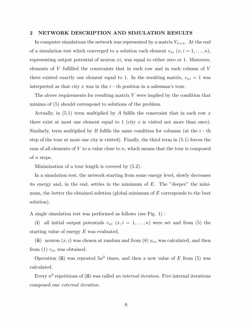
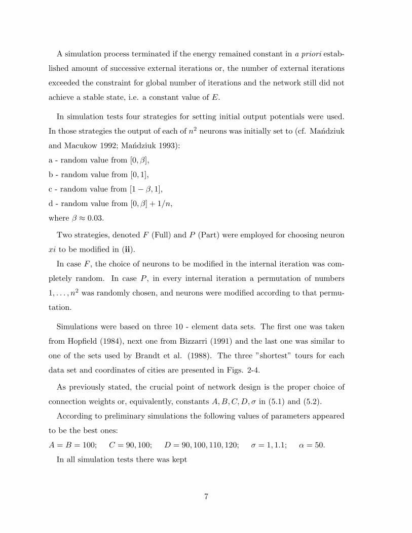
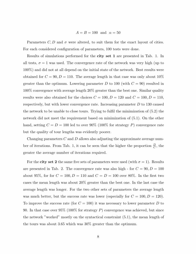
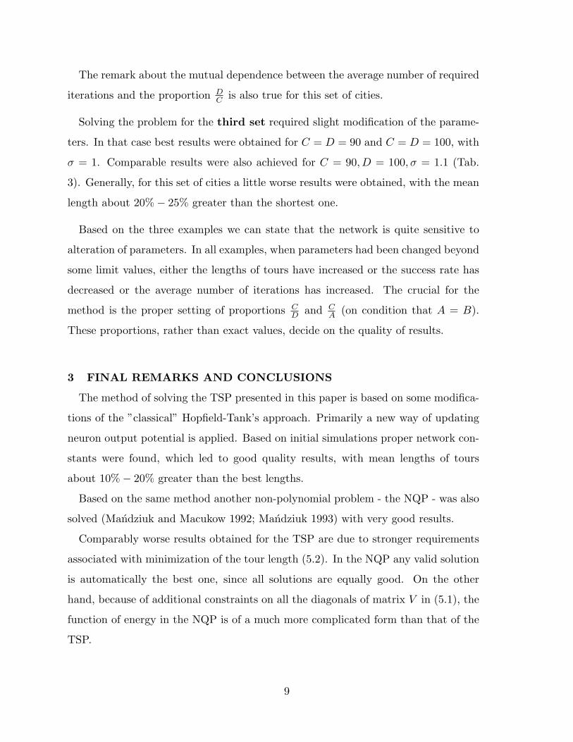
Simulations were based on three 10 - element data sets. The first one was taken

from Hopfield (1984), next one from Bizzarri (1991) and the last one was similar to

one of the sets used by Brandt et al. (1988). The three ”shortest” tours for each

data set and coordinates of cities are presented in Figs. 2-4.

As previously stated, the crucial point of network design is the proper choice of

connection weights or, equivalently, constants A,B, C, D, σ in (5.1) and (5.2).

According to preliminary simulations the following values of parameters appeared

to be the best ones:

A = B = 100; C = 90, 100; D = 90, 100, 110, 120; σ = 1, 1.1; α = 50.

In all simulation tests there was kept

7

A = B = 100 and α = 50

Parameters C, D and σ were altered, to suit them for the exact layout of cities.

For each considered configuration of parameters, 100 tests were done.

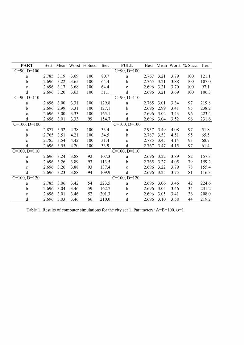
Results of simulations performed for the city set 1 are presented in Tab. 1. In

all tests, σ = 1 was used. The convergence rate of the network was very high (up to

100%) and did not at all depend on the initial state of the network. Best results were

obtained for C = 90, D = 110. The average length in that case was only about 10%

greater than the optimum. Lowering parameter D to 100 (with C = 90) resulted in

100% convergence with average length 20% greater than the best one. Similar quality

results were also obtained for the choices C = 100, D = 120 and C = 100, D = 110,

respectively, but with lower convergence rate. Increasing parameter D to 130 caused

the network to be unable to close tours. Trying to fulfil the minimization of (5.2) the

network did not meet the requirement based on minimization of (5.1). On the other

hand, setting C = D = 100 led to over 90% (100% for strategy P ) convergence rate

but the quality of tour lengths was evidently poorer.

Changing parameters C and D allows also adjusting the approximate average num-

ber of iterations. From Tab. 1, it can be seen that the higher the proportion DC , the

greater the average number of iterations required.

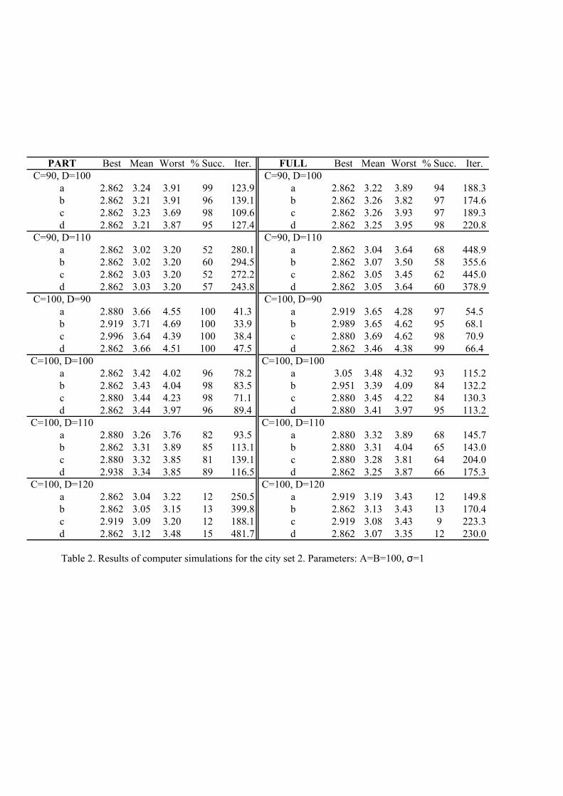
For the city set 2 the same five sets of parameters were used (with σ = 1). Results

are presented in Tab. 2. The convergence rate was also high - for C = 90, D = 100

about 95%, for for C = 100, D = 110 and C = D = 100 over 80%. In the first two

cases the mean length was about 20% greater than the best one. In the last case the

average length was longer. For the two other sets of parameters the average length

was much better, but the success rate was lower (especially for C = 100, D = 120).

To improve the success rate (for C = 100) it was necessary to lower parameter D to

90. In that case over 95% (100% for strategy P ) convergence was achieved, but since

the network ”worked” mostly on the syntactical constraint (5.1), the mean length of

the tours was about 3.65 which was 30% greater than the optimum.

8

The remark about the mutual dependence between the average number of required

iterations and the proportion DC is also true for this set of cities.

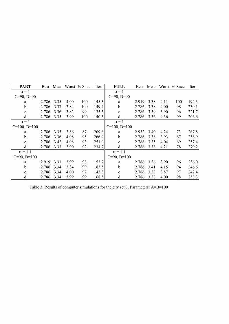
Solving the problem for the third set required slight modification of the parame-

ters. In that case best results were obtained for C = D = 90 and C = D = 100, with

σ = 1. Comparable results were also achieved for C = 90, D = 100, σ = 1.1 (Tab.

3). Generally, for this set of cities a little worse results were obtained, with the mean

length about 20%− 25% greater than the shortest one.

Based on the three examples we can state that the network is quite sensitive to

alteration of parameters. In all examples, when parameters had been changed beyond

some limit values, either the lengths of tours have increased or the success rate has

decreased or the average number of iterations has increased. The crucial for the

method is the proper setting of proportions CD and C

A (on condition that A = B).

These proportions, rather than exact values, decide on the quality of results.

3 FINAL REMARKS AND CONCLUSIONS

The method of solving the TSP presented in this paper is based on some modifica-

tions of the ”classical” Hopfield-Tank’s approach. Primarily a new way of updating

neuron output potential is applied. Based on initial simulations proper network con-

stants were found, which led to good quality results, with mean lengths of tours

about 10%− 20% greater than the best lengths.

Based on the same method another non-polynomial problem - the NQP - was also

solved (Mandziuk and Macukow 1992; Mandziuk 1993) with very good results.

Comparably worse results obtained for the TSP are due to stronger requirements

associated with minimization of the tour length (5.2). In the NQP any valid solution

is automatically the best one, since all solutions are equally good. On the other

hand, because of additional constraints on all the diagonals of matrix V in (5.1), the

function of energy in the NQP is of a much more complicated form than that of the

TSP.

9

Good results obtained for both problems indicate that after more research the pro-

posed method may be applied to the wide subset of NP-Hard optimization problems.

The very good point of the introduced method is its independence on the initial

state of the network. All four ways of setting the starting point of the network,

resulted in similar quality of success rates and mean lengths of obtained tours.

There are, however, some open questions. In further research we plan to completely

discretize the network, i.e. allow output potentials to take on values only from the

set {0, 1}. We are not yet sure if the results would be of as high quality as they were

for the NQP (Mandziuk 1993; Mandziuk 1995).

Our interest is also associated with a theoretical analysis of an influence of network

parameters on network behavior.

References

- Bizzarri AR, (1991) Convergence properties of a modified Hopfield-Tank model.

Biol. Cybern. 64, 293-300

- Brandt RD, Wang Y, Laub AJ, Mitra SK, (1988) Alternative Networks for Solving

the Traveling Salesman Problem and the List-Matching Problem. ICNN, 333-340

- Dantzig GB, Fulkerson DR, Johnson SM, (1954) Solutions of a Large-Scale

Traveling-Salesman Problem, Operations Research 2, 393-410

- Dantzig GB, Fulkerson DR, Johnson SM, (1959) On a linear programming combi-

natorial approach to the traveling salesman problem, Operations Research 7, 58-66

- Hopfield JJ, (1984) Neurons with graded response have collective computational

properties like those of two-state neurons. Proc. Natl. Acad. Sci. USA 81, 3088-

3092

- Hopfield JJ, Tank DW, (1985) ”Neural” Computation of Decisions in Optimization

Problems. Biol. Cybern 52, 141-152

10

- Kamgar-Parsi B, Kamgar-Parsi B, (1990) On Problem Solving with Hopfield Neural

Networks. Biol. Cybern. 62, 415-423

- Lin S, Kernighan BW, (1973) An Effective Algorithm for the Traveling Salesman

Problem, Operations Research 21, 498-516

- Mandziuk J, (1993) Application of neural networks to solving some optimization

problems. Ph.D. Thesis, Warsaw University of Technology (in Polish)

- Mandziuk J, (1995) Solving the N-Queens Problem with a binary Hopfield-type

network. Synchronous and asynchronous model. Biol. Cybern. (in press)

- Mandziuk J, Macukow B, (1992) A Neural Network Designed to Solve The N-Queens

Problem. Biol. Cybern. 66, 375-379

- Padberg M, Rinaldi G, (1987) Optimization Of A 512-City Symmetric Traveling

Salesman Problem By Branch And Cut, Operations Research Letters 6, 1-7

- Reingold EM, Nievergelt J, Deo N, (1985) Algorytmy kombinatoryczne, PWN

- Wilson GV, Pawley GS, (1988) On the stability of the Travelling Salesman problem

algorithm of Hopfield and Tank. Biol. Cybern. 58, 63-70

- Yao KC, Chavel P, Meyrueis P, (1989) Perspective of a neural optical solution to the

Traveling Salesman optimization Problem. SPIE, 1134, Optical Pattern Recogni-

tion ll, 17-25

11

igure 1: A diagram of dynamical evolution of the network.

output

5*n iterations2

until E remains constant in 5 successive iterationsor the number of iterations exceedes 25

V Eij0, 0 Uij Vij E

F

X YA 0.25 0.16B 0.85 0.35C 0.65 0.24D 0.70 0.50E 0.15 0.22F 0.25 0.78G 0.40 0.45H 0.90 0.65I 0.55 0.90J 0.60 0.28

Figure 2. City set 1: cities coordinates and the shortest tour

City set 1

0,00

0,20

0,40

0,60

0,80

1,00

0,00 0,20 0,40 0,60 0,80 1,00

EA

J

C

B

D

H

I

F

G

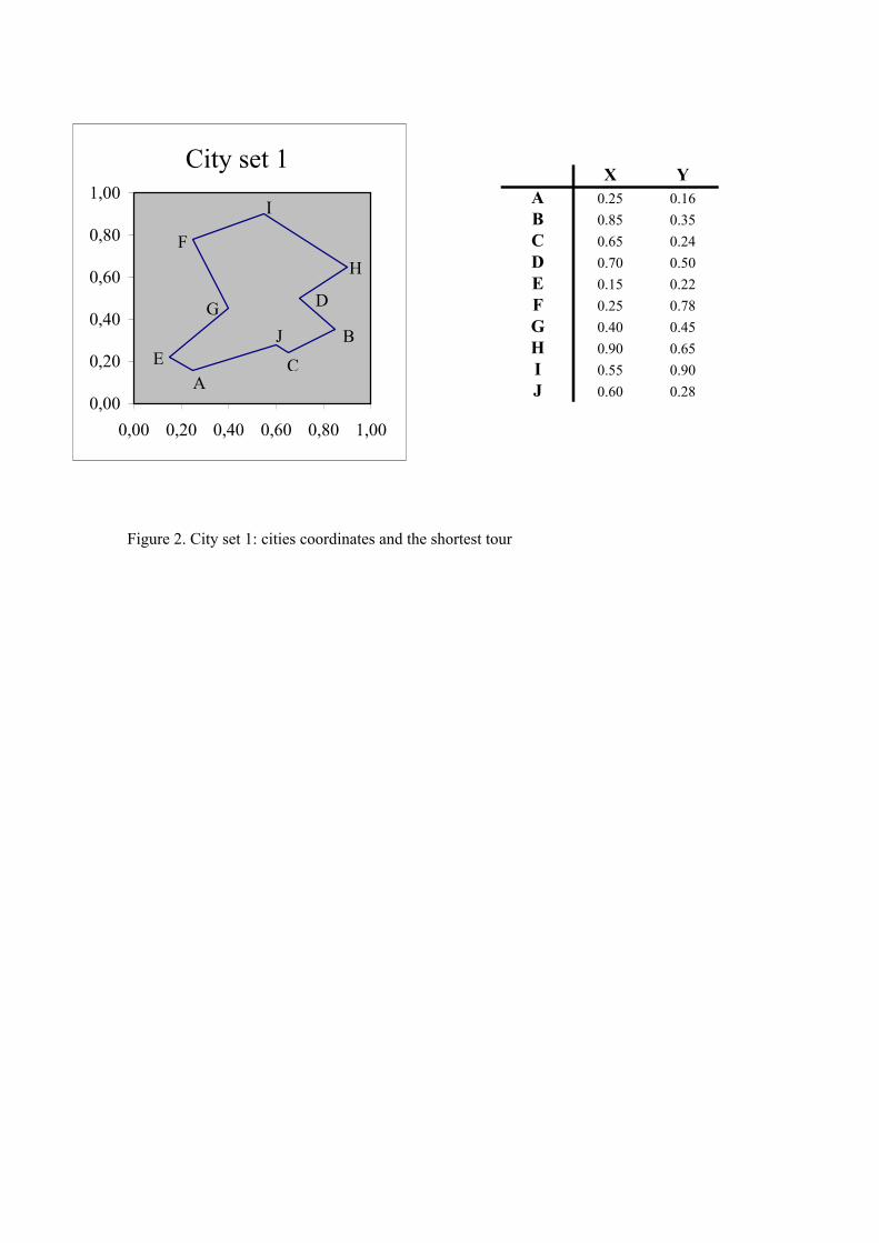
X YA 0.025 0.125B 0.150 0.750C 0.125 0.225D 0.325 0.550E 0.500 0.150F 0.625 0.500G 0.700 0.375H 0.875 0.400I 0.900 0.425J 0.925 0.700

Figure 3. City set 2: cities coordinates and the shortest tour

City set 2

0,000,100,200,300,400,500,600,700,80

0,00 0,20 0,40 0,60 0,80 1,00

D F

J

HIG

E

B

A

C

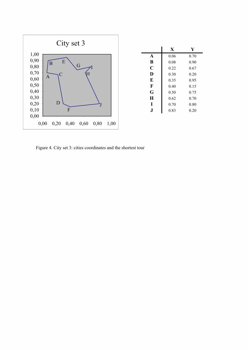
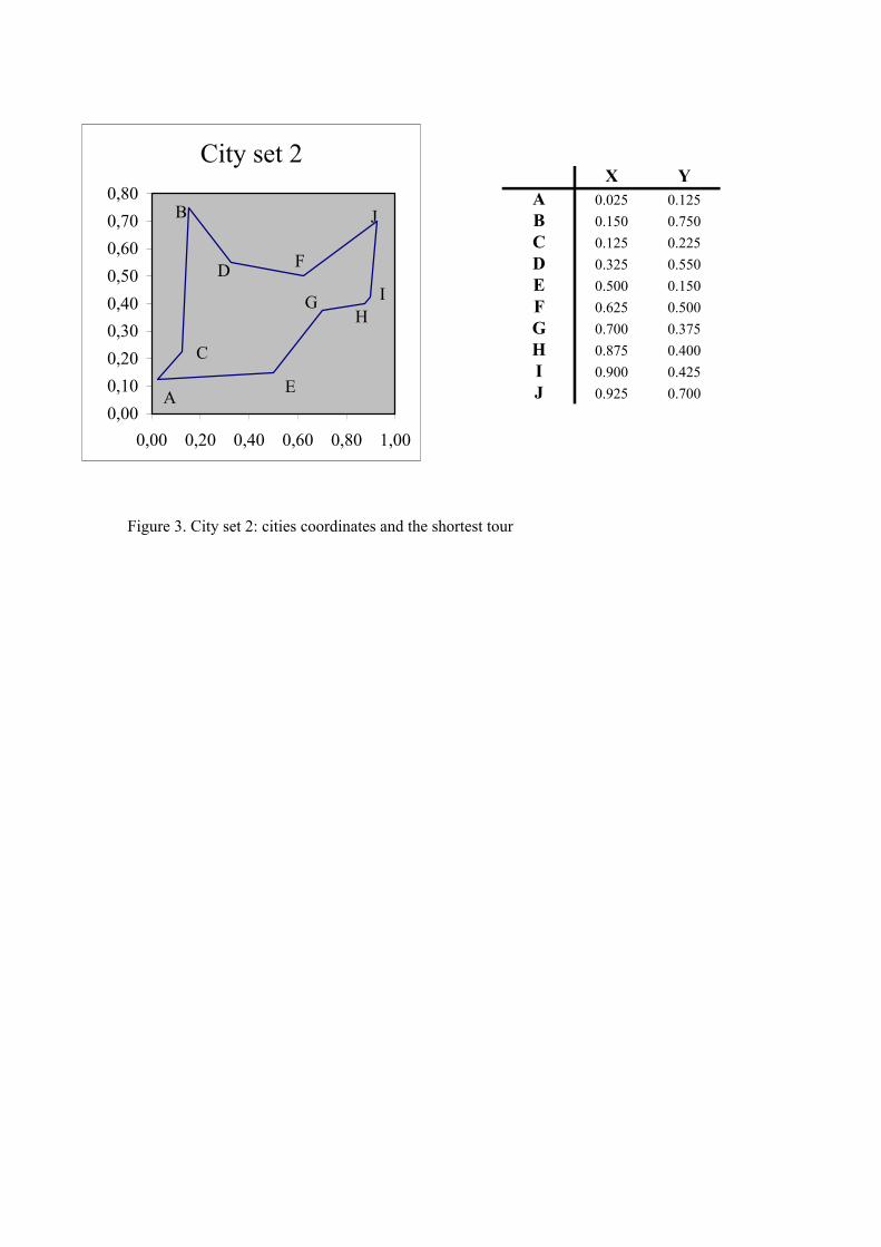
X YA 0.06 0.70B 0.08 0.90C 0.22 0.67D 0.30 0.20E 0.35 0.95F 0.40 0.15G 0.50 0.75H 0.62 0.70I 0.70 0.80J 0.83 0.20

Figure 4. City set 3: cities coordinates and the shortest tour

City set 3

0,000,100,200,300,400,500,600,700,800,901,00

0,00 0,20 0,40 0,60 0,80 1,00

DF

J

HIG

EB

A C

PART Best Mean Worst % Succ. Iter. FULL Best Mean Worst % Succ. Iter.C=90, D=100 C=90, D=100

a 2.785 3.19 3.69 100 80.7 a 2.767 3.21 3.79 100 121.1b 2.696 3.22 3.65 100 64.4 b 2.765 3.21 3.88 100 107.0c 2.696 3.17 3.68 100 64.4 c 2.696 3.21 3.70 100 97.1d 2.696 3.20 3.63 100 51.1 d 2.696 3.21 3.69 100 106.3

C=90, D=110 C=90, D=110a 2.696 3.00 3.31 100 129.8 a 2.765 3.01 3.34 97 219.8b 2.696 2.99 3.31 100 127.1 b 2.696 2.99 3.41 95 238.2c 2.696 3.00 3.33 100 165.1 c 2.696 3.02 3.43 96 223.4d 2.696 3.01 3.33 99 154.7 d 2.696 3.04 3.52 96 231.6

C=100, D=100 C=100, D=100a 2.877 3.52 4.38 100 33.4 a 2.937 3.49 4.08 97 51.8b 2.765 3.51 4.21 100 34.5 b 2.787 3.53 4.51 95 65.5c 2.785 3.54 4.42 100 31.4 c 2.785 3.45 4.14 93 68.7d 2.696 3.55 4.20 100 33.9 d 2.767 3.47 4.15 97 61.4

C=100, D=110 C=100, D=110a 2.696 3.24 3.88 92 107.3 a 2.696 3.22 3.89 82 157.3b 2.696 3.26 3.89 93 113.5 b 2.765 3.27 4.05 79 159.2c 2.696 3.26 3.88 93 137.4 c 2.696 3.22 3.79 78 155.4d 2.696 3.23 3.88 94 109.9 d 2.696 3.25 3.75 81 116.3

C=100, D=120 C=100, D=120a 2.785 3.06 3.42 54 223.5 a 2.696 3.06 3.46 42 224.6b 2.696 3.04 3.46 59 162.7 b 2.696 3.05 3.46 34 231.2c 2.696 3.01 3.46 52 201.3 c 2.696 3.05 3.41 36 208.0d 2.696 3.03 3.46 66 210.0 d 2.696 3.10 3.58 44 219.2

Table 1. Results of computer simulations for the city set 1. Parameters: A=B=100, σ=1

PART Best Mean Worst % Succ. Iter. FULL Best Mean Worst % Succ. Iter.C=90, D=100 C=90, D=100

a 2.862 3.24 3.91 99 123.9 a 2.862 3.22 3.89 94 188.3b 2.862 3.21 3.91 96 139.1 b 2.862 3.26 3.82 97 174.6c 2.862 3.23 3.69 98 109.6 c 2.862 3.26 3.93 97 189.3d 2.862 3.21 3.87 95 127.4 d 2.862 3.25 3.95 98 220.8

C=90, D=110 C=90, D=110a 2.862 3.02 3.20 52 280.1 a 2.862 3.04 3.64 68 448.9b 2.862 3.02 3.20 60 294.5 b 2.862 3.07 3.50 58 355.6c 2.862 3.03 3.20 52 272.2 c 2.862 3.05 3.45 62 445.0d 2.862 3.03 3.20 57 243.8 d 2.862 3.05 3.64 60 378.9

C=100, D=90 C=100, D=90a 2.880 3.66 4.55 100 41.3 a 2.919 3.65 4.28 97 54.5b 2.919 3.71 4.69 100 33.9 b 2.989 3.65 4.62 95 68.1c 2.996 3.64 4.39 100 38.4 c 2.880 3.69 4.62 98 70.9d 2.862 3.66 4.51 100 47.5 d 2.862 3.46 4.38 99 66.4

C=100, D=100 C=100, D=100a 2.862 3.42 4.02 96 78.2 a 3.05 3.48 4.32 93 115.2b 2.862 3.43 4.04 98 83.5 b 2.951 3.39 4.09 84 132.2c 2.880 3.44 4.23 98 71.1 c 2.880 3.45 4.22 84 130.3d 2.862 3.44 3.97 96 89.4 d 2.880 3.41 3.97 95 113.2

C=100, D=110 C=100, D=110a 2.880 3.26 3.76 82 93.5 a 2.880 3.32 3.89 68 145.7b 2.862 3.31 3.89 85 113.1 b 2.880 3.31 4.04 65 143.0c 2.880 3.32 3.85 81 139.1 c 2.880 3.28 3.81 64 204.0d 2.938 3.34 3.85 89 116.5 d 2.862 3.25 3.87 66 175.3

C=100, D=120 C=100, D=120a 2.862 3.04 3.22 12 250.5 a 2.919 3.19 3.43 12 149.8b 2.862 3.05 3.15 13 399.8 b 2.862 3.13 3.43 13 170.4c 2.919 3.09 3.20 12 188.1 c 2.919 3.08 3.43 9 223.3d 2.862 3.12 3.48 15 481.7 d 2.862 3.07 3.35 12 230.0

Table 2. Results of computer simulations for the city set 2. Parameters: A=B=100, σ=1

PART Best Mean Worst % Succ. Iter. FULL Best Mean Worst % Succ. Iter.σ = 1 σ = 1

C=90, D=90 C=90, D=90a 2.786 3.35 4.00 100 145.3 a 2.919 3.38 4.11 100 194.3b 2.786 3.37 3.84 100 149.4 b 2.786 3.38 4.00 98 230.1c 2.786 3.36 3.82 99 135.5 c 2.786 3.39 3.90 96 221.7d 2.786 3.35 3.99 100 140.5 d 2.786 3.36 4.36 99 206.6

σ = 1 σ = 1C=100, D=100 C=100, D=100

a 2.786 3.35 3.86 87 209.6 a 2.932 3.40 4.24 73 267.8b 2.786 3.36 4.08 95 266.9 b 2.786 3.38 3.93 67 236.9c 2.786 3.42 4.08 93 251.0 c 2.786 3.35 4.04 69 257.4d 2.786 3.33 3.90 92 234.7 d 2.786 3.38 4.21 78 279.2

σ = 1.1 σ = 1.1C=90, D=100 C=90, D=100

a 2.919 3.31 3.99 98 153.7 a 2.786 3.36 3.90 96 236.0b 2.786 3.34 3.84 99 183.5 b 2.786 3.41 4.15 94 246.6c 2.786 3.34 4.00 97 143.3 c 2.786 3.33 3.87 97 242.4d 2.786 3.34 3.99 99 168.5 d 2.786 3.38 4.00 98 258.3

Table 3. Results of computer simulations for the city set 3. Parameters: A=B=100