JOURNAL OF OPTIMIZATION THEORY AND APPLICATIONS: Vol. 105, No. 3, pp. 707–730, JUNE 2000

Solving the Unit Commitment Problem by aUnit Decommitment Method1,2

C. L. TSENG,3 C. A. LI,4 AND S. S. OREN5

Abstract. In this paper, we present a unified decommitment methodto solve the unit commitment problem. This method starts with a solu-tion having all available units online at all hours in the planning horizonand determines an optimal strategy for decommitting units one at atime. We show that the proposed method may be viewed as an approxi-mate implementation of the Lagrangian relaxation approach and thatthe number of iterations is bounded by the number of units. Numericaltests suggest that the proposed method is a reliable, efficient, and robustapproach for solving the unit commitment problem.

Key Words. Power system scheduling, unit commitment, unit decom-mitment, mixed-integer programming, Lagrangian relaxation, heuristicprocedures.

1. Introduction

A problem that must be solved frequently by a power utility is to deter-mine economically a schedule of what units will be used to meet the fore-casted demand and operating constraints, such as spinning reserverequirements, over a short time horizon. This problem is commonly referredto as the unit commitment (UC) problem. The UC problem is a mixed-integerprogramming problem and is in the class of NP-hard problems (Ref. 1).

Because of its size and NP-hardness, the true optimal solution of theUC problem is normally difficult to obtain. Many optimization methods

1This paper is dedicated by Shmuel S. Oren to David G. Luenberger, his thesis adviser, inspir-ing teacher, and colleague who introduced him to the field of optimization.

2This work was supported in part by the National Science Foundation, Grant IRI-9120074.3Assistant Professor, Department of Civil Engineering, University of Maryland, College Park,Maryland.

4Consultant, Pacific Gas and Electric Company, San Francisco, California.5Professor, Department of Industrial Engineering and Operations Research, University ofCalifornia at Berkeley, Berkeley, California.

7070022-3239y00y0600-0707$18.00y0 2000 Plenum Publishing Corporation

JOTA: VOL. 105, NO. 3, JUNE 2000708

have been proposed to solve the UC problem. For example, we mention thepriority list method (Ref. 2), branch-and-bound methods (Refs. 3–5),dynamic programming approaches (Refs. 6–8), and Lagrangian relaxation(LR) methods (e.g. Refs. 9–11). For a detailed review, the reader is referredto Ref. 12. Among them, the LR methods are the most advanced and widelyused approaches. Though popular, the LR approaches are known to requiremany heuristics which strongly influence their performance (Refs. 12–13).

There are also heuristic methods. For example, Lee develops in Ref.14, a method which sequentially determines the commitment of the nextmost-advantageous unit to commit; the decision making involves a priceadjustment, which resembles a bidding process. Also in Ref. 15, Li et al.proposed a method which mimics the LR approach; the multipliers aretaken from the economic dispatch phase, rather than updated by the sub-gradient iteration. In Ref. 16, a unit decommitment (UD) method was devel-oped as a postprocessing tool to improve the solution quality of the existingUC algorithms.

In this paper, we consolidate the approaches presented in Refs. 15–16and extend them to a more general formulation. The proposed method is aunified unit decommitment method. This method starts with a solution hav-ing all available units online at all hours in the planning horizon and deter-mines an optimal strategy for decommitting units, one at a time. We showthat the proposed method may be viewed as an approximate implemen-tation of the LR approach. The multiplier updating rule is similar to thatin Ref. 15. Furthermore, we show that the number of iterations required bythe method is bounded by the number of units. Empirical tests suggest thatthe proposed method is efficient and robust.

This paper is organized as follows. In Section 2, the UC problem isformulated. Section 3 presents some properties of economic dispatch. Wegeneralize the UD method and propose an algorithm for solving the UCproblem using the UD method in Section 4. The relation between the pro-posed method and the LR approach is discussed in Section 5. Finally, wegenerate random instances of UC problems and solve them by the proposedmethod. Numerical test results and conclusions are given in Section 6.

2. Problem Formulation

In this paper, the following standard notations will be used. Additionalsymbols will be introduced when necessary.

iGindex for number of units, iG1, . . . , I;tGindex for time, tG0, . . . , T;

JOTA: VOL. 105, NO. 3, JUNE 2000 709

uitGzero–one decision variable indicating whether unit iis up or down in time period t;

xitG state variable indicating the length of time that uniti has been up or down in time period t;

toni [toff

i ]Gminimum number of periods unit i must remain on[off ] after it has been turned on [off ];

tcoldi Gnumber of periods required for the boiler of unit i

to cool down;pitGstate variable indicating the amount of power unit i

is generating in time period t;pmin

i [pmaxi ]Gminimum [maximum] rated capacity of unit i;rmax

i Gmaximum reserve for unit i;ri(pit) ≡ min(rmax

i , pmaxi Apit), reserve available from unit i in

time period t;Ci (pit )Gfuel cost for operating unit i at output level pit in

time period t, assumed to be smooth, increasing,and strictly convex;

Si (xi,tA1 , uit , ui,tA1)G startup cost associated with turning on unit i at thebeginning of time period t;

DtGforecast demand in time period t;RtGspinning reserve requirement in time period t.

The unit commitment (UC) problem is formulated as the followingmixed-integer programming problem:

minu,x,p

∑T

tG1∑I

iG1[Ci (pit)uitCSi (xi,tA1 , uit , ui,tA1)], (1)

subject to the demand constraints

∑I

iG1pituitGDt , tG1, . . . , T, (2)

and the spinning reserve constraints

∑I

iG1ri (pit)uit¤Rt , tG1, . . . , T, (3)

where

ri (pit) ≡ min(rmaxi , pmax

i Apit).

There are other unit constraints such as the unit capacity constraints

pmini ⁄pit⁄pmax

i , iG1, . . . , I and tG1, . . . , T, (4)

JOTA: VOL. 105, NO. 3, JUNE 2000710

the state transition equations for iG1, . . . , I,

xitG5min(toni , max(xi,tA1 , 0)C1), if uitG1,

max(−tcoldi , min(xi,tA1 , 0)A1), if uitG0,

(5)

the minimum upydown time constraints for iG1, . . . , I,

uitG51, if 1⁄xi,tA1Fton

i ,

0, if −1¤xi,tA1HAtoffi ,

0 or 1, otherwise,

(6)

and the initial conditions on xit at tG0 for ∀i.In the objective function, we assume that the fuel cost Ci of a unit to

be a smooth, increasing, and strictly convex function of the power output[MWh] of the unit. For each unit, the startup cost Si (xi,tA1 , uit , ui,tA1) is anincreasing function of the length of time that the unit has been off [i.e.,xi,tA1 ]. The state transition diagram is given in Fig. 1. To limit the size of

Fig. 1. Example of state transition diagram: tonG3, toffG2, t coldG4.

JOTA: VOL. 105, NO. 3, JUNE 2000 711

the state space, we assume that the increase of Si (xi,tA1 , uit , ui,tA1) is negli-gible when xi,tA1F−t cold

i , where t coldi Htoff

i is the unit cold time. To furthersimplify notation, we let

Si (u, t)GSi (xi,tA1 , uit , ui,tA1).

3. Reserve-Constrained Economic Dispatch

Given a known commitment uGuit satisfying (5)–(6), the UC prob-lem is reduced to a nonlinear program called economic dispatch (ED). EDis the problem of allocating system demand among all online generatingunits while satisfying (2)–(4) at any time over the planning horizon, i.e., todetermine the corresponding pG pit. In this paper, a tilde superscriptdenotes fixed realization of the corresponding variable. Since ED is separ-able in time, it can be solved sequentially by hour t. If the spinning reserveconstraints (3) are not considered, at each time t the ED problem is a con-ventional resource allocation (RA) problem (e.g. Ref. 17), which has thefollowing form:

min ∑i∈J

Ci (pi), (7a)

s.t. ∑i∈J

piGD, (7b)

pmini ⁄pi⁄pmax

i , ∀i∈J, (7c)

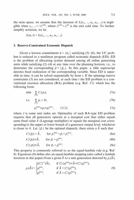
where J is some unit index set. Optimality of such RA-type ED problemrequires that all generators operate at a marginal cost that either equalssame fixed value λ (Lagrange multiplier) or equals the marginal cost corre-sponding to the upper or lower bound of a generator output level, whicheveris closer to λ . Let pi be the optimal dispatch; there exists a λ such that

C ′i ( pi)Gλ , for pmini FpiFpmax

i , (8a)

C′i ( pi)¤λ , for piGpmini , (8b)

C′i ( pi)⁄λ , for piGpmaxi . (8c)

This property is commonly referred to as the equal-lambda rule (e.g. Ref.8). Equations (8) define also an equal-lambda mapping (also called a lambdaiteration in this paper) from a given λ to a unit generation denoted by pi (λ ),

pi (λ)G5(C′i )−1(λ), if C ′i (pmin

i )⁄λ⁄C ′i (pmaxi ),

pmini , if λFC′i (pmin

i ),

pmaxi , if λHC′i (pmax

i ).

(9)

JOTA: VOL. 105, NO. 3, JUNE 2000712

Another approach for solving the RA-type ED problem is called thedual approach, which performs iterations on the lambda domain using themapping (9) and terminates when the relation

∑i∈J

pi(λ)GD (10)

is satisfied. In this paper, we will use the term ‘‘equal-lambda method’’ torefer to a method which solves the RA-type ED problem using the dualapproach. An equal-lambda method can be implemented very efficientlysuch that it obtains the optimal solution within strongly polynomial time ifthe functions Ci ( ·) are quadratic convex (Ref. 18).

With the presence of the reserve constraints (3), the problem is areserve-constrained economic dispatch (RCED). Methods for obtainingapproximate solutions for RCED were proposed in Refs. 19–20. In thissection, we state some mathematical properties of RCED. Define the indexset of online units at time t with respect to this feasible commitment,

J(t; u) ≡ i u uitG1.

For simplicity, let

JtGJ(t; u).

The RCED problem in time t is denoted by

(RCED) rced(Jt , t) ≡ min ∑i∈Jt

Ci ( pit), (11a)

s.t. ∑i∈Jt

pitGDt , (11b)

∑i∈Jt

rit( pit)¤Rt , (11c)

pmini ⁄pit⁄pmax

i , ∀i∈Jt . (11d)

Also, assume that pG pit solves rced(Jt , t), if the solution exists.

Proposition 3.1. The solution of RCED exists if and only if the follow-ing conditions hold:

∑i∈Jt

pmini ⁄Dt⁄ ∑

i∈Jt

pmaxi ARt , (12a)

∑i∈Jt

rmaxi ¤Rt . (12b)

JOTA: VOL. 105, NO. 3, JUNE 2000 713

Proof. The ‘‘only if ’’ part is obvious. To show the ‘‘if ’’ part, note that(12b) implies that there exist ri such that

∑i∈Jt

riGRt , 0⁄ri⁄rmaxi , ∀i∈Jt .

Since

∑i∈Jt

pmini ⁄Dt⁄ ∑

i∈Jt

pmaxi ARtG ∑

i∈Jt

(pmaxi Ari),

there exist pit such that

∑i∈Jt

pitGDt ,

and

pmini ⁄pit⁄pmax

i Ari , ∀i∈Jt .

Note that

∑i∈Jt

ri ( pit)¤Rt;

so, pit is a feasible solution for RCED. h

In the sequel, we assume always that the conditions stated in Prop-osition 3.1 are satisfied; therefore, the optimal solution of RCED exists forall t.

Proposition 3.2. Given a commitment u, assume that pit is an opti-mal solution of the corresponding RCED. Then, there exist Ωt and Λt , twomutually exclusive and exhaustive subsets of Jt , i.e.,

Ωt∪ΛtGJt and Ωt∩ΛtG∅,

and Lagrange multipliers λ t , α t , µt ,, tG1, . . . , T, such that, for ∀i∈Ωt ,

C′i ( pit)Gα t , for pmaxi Armax

i FpitFpmaxi , (13a)

C′i ( pit)⁄αt , for pitGpmaxi , (13b)

and for ∀i∈Λt ,

C′i ( pit)Gλ t , for pmini FpitFpmax

i Armaxi , (14a)

C′i ( pit)⁄λ t , for pitGpmaxi Armax

i , (14b)

C′i ( pit)¤λ t , for pitGpmini , (14c)

JOTA: VOL. 105, NO. 3, JUNE 2000714

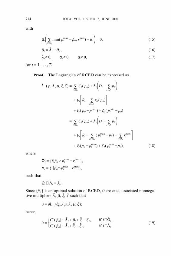
with

µt1 ∑i∈Jt

min( pmaxi Apit , rmax

i )ARt2G0, (15)

µtGλ tAα t , (16)

λ t¤0, α t¤0, µt¤0, (17)

for tG1, . . . , T.

Proof. The Lagrangian of RCED can be expressed as

L ( p, λ , µ, ξ, ζ)G ∑i∈Jt

Ci ( pit)Cλ t1DtA ∑i∈Jt

pit2Cµt3RtA ∑

i∈Jt

rit ( pit)4Cξt ( pitApmax

i )Cζ t ( pmini Apit)

G ∑i∈Jt

Ci ( pit)Cλ t1DtA ∑i∈Jt

pit2Cµt3RtA ∑

i∈Ωt

( pmaxi Apit)A ∑

i∈Λt

rmaxi 4

Cξt (pitApmaxi )Cζ t ( pmin

i Apit), (18)

where

ΩtGi u pitHpmaxi Armax

i ,

ΛtGi u pit⁄pmaxi Armax

i ,

such that

Ωt∪ΛtGJt .

Since pit is an optimal solution of RCED, there exist associated nonnega-tive multipliers λ , µ, ξ, ζ such that

0G∂L y∂pit ( p, λ , µ, ξ);

hence,

0G5C′i ( pit)Aλ tCµtCξtAζ t , if i∈Ωt ,

C′i ( pit)Aλ tCξtAζ t , if i∈Λt .(19)

JOTA: VOL. 105, NO. 3, JUNE 2000 715

Note that at least one of ξt and ζ t must equal zero, depending on whetherpit ≠ pmin

i or pit ≠ pmaxi is met, respectively. Let

α tGλ tAµt;

thus, (19) reduces to (13) and (14). Because of the assumption that Ci isincreasing, α t¤0. Equation (15) is the so-called complementary slacknesscondition. h

An intuitive way to interpret the optimality condition is to divide theunits into two categories: Λt is the set of units with cheap reserve but expens-ive generation, and Ωt is the counterpart. Based on the result of Proposition3.2, we have the following modified equal-lambda method for solvingRCED.

Modified Equal-Lambda Method for Solving RCED. Initially, setlambda equal to zero; by (9), all units generate at their minimum ratedcapacity, i.e.,

pitGpmini , i∈Jt .

The system now is overreserved, but undergenerated. Gradually increasinglambda will increase system generation and simultaneously decrease systemreserve. Let lambda be gradually increased until either the demand con-straint (2) or the equality of the reserve constraint (3) is satisfied, whicheveroccurs first. At this point, assume that pit is the corresponding unit gener-ation. There are two cases.

Case 1. Demand Constraint Is Met First. This corresponds to anoverreserved system. Let

ΩtGi u pitHpmaxi Armax

i , ΛtGi u pit⁄pmaxi Armax

i .

Denote the value of lambda by λ t . By (15), µtG0, i.e., α tGλ t . It can be seeneasily that the optimality conditions stated in Proposition 3.2 are satisfied.

Case 2. Equality of Reserve Constraint Is Met First. Denote thevalue of lambda by α t . Let Ωt and Λt be defined as in Case 1. In order toinduce more generation to satisfy the demand constraint while maintainingthe reserve, the generations of units in Ωt should remain fixed and only thegenerations of units in Λt are increased by increasing lambda, until thedemand constraint is satisfied. Note that, during the lambda iterationsapplied to units in Λt , the capacities of units in Λt are further bounded fromabove by pmax

i Armaxi in order to maintain reserve. Denote the final value of

JOTA: VOL. 105, NO. 3, JUNE 2000716

Fig. 2. Illustration of the modified equal lambda method, ΩtG1, 2.

lambda by λ t . By definition,

µtGλ tAα t¤0. h

In Fig. 2, an illustration of the modified equal-lambda method (Case2) is given. Seven units are considered. For each unit, the pit axis is sup-pressed and only the C ′( pit ) axis is shown, since they are in one-to-onecorrespondence. When lambda is gradually increased from 0 to α t , equalityof the reserve constraint is met first. Units 1 and 2 belong to Ωt , and theother units are in Λt . For the units in Λt , the value of lambda continues tobe raised until λ t . Since the upper bound of the generation capacity of uniti∈Λt has been reduced to pmax

i Armaxi , though λ tHC′i ( pmax

i Armaxi ), units 4

and 7 still generate at the level of pmaxi Armax

i .

Proposition 3.3. The modified equal-lambda method guarantees tofind a set of generation pit, associated with multipliers λ t, and µt,satisfying the optimality condition stated in Proposition 3.2.

Proof. First, we need to show that, in Case 2, the lambda iterationswould terminate with the demand constraint (2) satisfied. Assume on the

JOTA: VOL. 105, NO. 3, JUNE 2000 717

contrary that this would not happen. It implies that

DtH ∑i∈Ωt

pitC ∑i∈Λt

(pmaxi Armax

i )

¤ ∑i∈Ωt

(pmaxi Armax

i )C ∑i∈Λt

(pmaxi Armax

i )

¤ ∑i∈Jt

pmaxi A∑

Jt

rmaxi

¤ ∑i∈Jt

pmaxi ARt [by (12b)]. (20)

Inequality (20) violates (12). This is a contradiction. Secondly, we need toshow that the obtained pit and λ t, µt, α t satisfy the optimalityconditions in Proposition 3.2. This part is straightforward and is omitted.Since the RCED problem involves the minimization of a strictly convexfunction over a convex set, the solution obtained is the unique and globalone. h

Note that, in the modified equal-lambda method, we do not emphasizeimplementation issues. We intend to interpret how one arrives at the opti-mality conditions. The purpose is to develop the proposition given in thefollowing section.

3.1. Postoptimality Analysis. In Proposition 3.2, λ t and µt arethe Lagrange multipliers for the constraints (2) and (3), respectively. Giventhat pit associated with λ t and µt solves rced(Jt , t), suppose thatj∈Jt . To know whether Jt \ j is a more economic commitment in time t(ignoring other physical constraints, e.g., minimum uptime constraints atthis point), one can either directly evaluate rced(Jt \ j, t) or estimate theincreased dispatch cost due to the decommitment of unit j in time t usingthe Lagrange multipliers λ t and µt, and then compare with the savedcost Cj ( pjt ). We investigate next the latter approach.

Proposition 3.4. Suppose that pit is the optimal solution torced(Jt , t) and j∈Jt . After decommitting unit j in time t, suppose thatpitC∆pit , for ∀i∈Jt \ j, solve rced(Jt \ j, t). If at time t, the system is notoverreserved (i.e., the reserve constraint is achieved at equality), the follow-ing properties of ∆pit are true:

(i) ∑i∈Jt \ j

∆pitGp jt;

(ii) ∆pit⁄0, for ∀i∈Ωt \ j,

JOTA: VOL. 105, NO. 3, JUNE 2000718

∆pit¤0, for ∀i∈Λt \ j;

(iii) pitC∆pitGpmaxi Armax

i , for i∈Λ′t \ ΛtG(Ωt \ j)\Ω′t ;

(iv) ∑i∈Ωt \ j

∆pitCrj ( p jt)G0.

Proof. Since the modified equal-lambda method presented in the pre-vious section has been shown to be able to locate the unique solution ofRCED, we shall use it to prove these properties. Property (i) is due to theload balance equation. Since it is assumed that the system is not over-reserved, applying the modified equal-lambda method to the system withunit j decommitted, Case 2 will continue to prevail. Let the primed variables(e.g. p ′it , α ′t , Λ′t , Ω′t) be the obvious corresponding notations in the decom-mitted system (e.g. p ′itGpitC∆pit). Because the decommitted system has lessreserve capability, α ′t⁄α t and Ω′t ⊆ Ωt in order to induce more reserve.Therefore, p′it⁄pit , i.e.

∆pit⁄0, for ∀i∈Ω′t;

and p ′it⁄pmaxi Armax

i ⁄pit , i.e.

∆pit⁄0, for i∈Ωt \Ω′t .

Similarly, to satisfy the load balance equation, λ ′t¤λ t and Λt \ j ⊆ Λ′t . So,

∆pit¤0, for i∈Λt \ j,

and (ii) is proved. Property (iii) follows immediately from the fact that

λ ′t¤λ t¤α t¤C′i (pmaxi Armax

i ), for ∀i∈Λ′t \ ΛtG(Ωt \ j)\Ω′t .

To prove property (iv), note that

RtGrj ( p jt)C ∑i∈Ωt \ j

(pmaxi Apit)C ∑

i∈Λt \ j

rmaxi

G ∑i∈Ω′t

(pmaxi Ap′it)C ∑

i∈Λ′t

rmaxi

G ∑i∈Ω′t

( pmaxi Ap′it)C ∑

i∈Λ′t \ Λt

rmaxi C ∑

i∈Λt \ jrmax

i

G ∑i∈Ω′t

( pmaxi Ap′it)C ∑

i∈(Ωt \ j)\Ω′t

rmaxi C ∑

i∈Λt \ j

rmaxi

G ∑i∈Ω′t

(pmaxi Ap′it)C ∑

i∈(Ωt \ j)\Ω′t

( pmaxi Ap′it)C ∑

i∈Λt\ j

rmaxi

G ∑i∈Ωt \ j

( pmaxi Ap′it)C ∑

i∈Λt \ jrmax

i . (21)

JOTA: VOL. 105, NO. 3, JUNE 2000 719

Comparing the first and last lines of (21), property (iv) follows. h

Again, properties (ii) and (iv) can be interpreted intuitively as follows:when decommitting unit j, the units in Ωt \ j, those with expensive reserve,decrease generation to make up the loss of reserve originally provided byunit j, while the units in Λt \ j, those with expensive generation, increasegeneration to balance the load.

Since all the fuel cost functions Ci are assumed smooth and convex, wecan estimate the increased cost due to the decommitment:

∑i∈Jt \ j

Ci ( pitC∆pit)ACi ( pit)

≈ ∑i∈Jt \ j

C′i ( pit)∆pit

≈λ t ∑i∈Λt \ j

∆pitC(λ tAµt) ∑i∈Ωt \ j

∆pit

Gλ t p jtAµt ∑i∈Ωt \ j

∆ pit

Gλ t p jtCµt rj ( p jt). (22)

Note that the approximation in the third line of (22) uses the result fromProposition 3.2, and that (22) is due to property (iv) in Proposition 3.4.Although (22) is derived under the assumption that the system is not over-reserved, it remains a good approximation when the system has excessivereserve capability. If the system is overreserved, Case 1 in the modifiedequal-lambda method will be encountered with µtG0. In this case, (22)reduces to the first-order approximation of the conventional ED problem(without reserve constraints). As will be shown in a later section, if thedecommitment process is repeated for multiple units, one at a time, eventu-ally Case 2 prevails, and obtains nonzero µt . Also, it can be further shownthat the two approximate relations (≈ ) in (22), second and third lines, canbe replaced by inequalities (¤ ).

4. Solving the Unit Commitment Using the Unit Decommitment

4.1. Unit Decommitment Method. In Section 3.1, given a feasible andeconomically dispatched schedule (u, p), we discussed how to estimate theincreased cost due to the decommitment of one unit. Now, we incorporateother physical constraints and present the problem of optimality improvinga unit’s schedule by decommitment. That is, in the time periods when theunit is already offline, it remains offline. The unit may be turned off in some

JOTA: VOL. 105, NO. 3, JUNE 2000720

online periods only if doing so can result in cost saving and does not causeproblem infeasibility. While we are improving a unit’s schedule, say unit j ’sschedule, by decommitment, other units’ commitments are kept fixed. Forexample, uit remains unchanged for ∀i ≠ j, ∀t, but pit are subject to changedue to the commitment of unit j. The formulation is as follows:

(Pj ) min ∑T

tG1

[Cj ( p jt)ujtC(λ t p jtCµt rj ( p jt))(1Aujt)CSj (u, t)], (23)

subject to

ujtG50, if u jtG0,

1, if u jtG1 and the removal of j from Jt

results in violation of (12),

0 or 1, otherwise,

(24)

and subject to the minimum uptime, downtime constraints and the initialconditions for unit j.

Note that in, (23), ujt and 1Aujt are two mutually exclusive decisions.If unit j is already online in time t (ujtG1), the generation cost is Cj ( pjt ); ifunit j is decommitted, the increased cost of the other units is approximatedby λ t pjtCµt rj ( pjt ). The startup cost of unit j is imposed whenever appli-cable. (Pj ) is an integer programming problem and can be solved using thefollowing dynamic programming recursive equations:

F (ujT, xjT)G0, (25a)

F (ujt , xjt)G min(uj,tC1 , xj,tC1)∈Wj

[Cj ( p jt)ujtC(λ t p jtCµt rj ( p jt))(1Aujt)

CSj (u, t)CF (uj,tC1 , xj,tC1)],

tG0, . . . , TA1, (25b)

where the decision space Wj is given by

WjG(1, x+) u1⁄x+⁄tonj , x+∈Z

∪(0, x−) uA1¤x−¤−tcoldj , x−∈Z. (26)

The optimal solution of (Pj ) is obtained from the last step of the dynamicprogramming algorithm as F (uj0 , xj0). In the above recurrence relation,F (ujt , xjt ) is known as the cost-to-go and defines the optimal cost for theremaining t periods, tG0, . . . , TA1. In this paper, the solution of (Pj ) iscalled the tentative commitment of unit j.

In the following algorithm, the superscript k denotes the kth iterationof the algorithm. Let Θk

i , iG1, . . . , I, be the total generating cost (fuel cost

JOTA: VOL. 105, NO. 3, JUNE 2000 721

and startup cost) of unit i of the feasible schedule (u k, p k); and let Θki , iG

1, . . . , I, be the optimal objective value of (P ki ) solved with respect to the

feasible solution (u k, p k). We now state the decommitment algorithm.

Algorithm 4.1. UD Algorithm.

Data. Feasible solution (u0 , p 0) is given.Step 0. Set k←0, evaluate Θ0

i , iG1, . . . , I.Step 1. Solve (P k

i ) with respect to (u k, p k) and obtain Θ ki for all iG

1, . . . , I.Step 2. Select a unit m such that Θk

mAΘkmH0. If there is no such a

unit, stop; otherwise, update the commitment of unit m in u k

by the tentative commitment obtained in (P km). The resultant

unit commitment is assigned to be u kC1.Step 3. Perform RCED on ukC1 to obtain pkC1 and evaluate ΘkC1

i ,the total generating cost of unit i, iG1, . . . , I.

Step 4. Set k←kC1, go to Step 1. h

The algorithm in Step 2 chooses the tentative commitment of a unitwhich can yield savings to replace the original commitment. That is, themethod corrects the unit commitment, one unit at a time. The followingproposition states some properties of the algorithm6.

Proposition 4.1. At time t, before unit i is decommitted, the followingstatements are true:

(i) If unit i is in Λt at some iteration, it will remain in Λt at sub-sequent iterations. If unit i is in Ωt , it may leave Ωt to join Λt atsome iteration and then remains there afterward.

(ii) λ kt ↑ , µk

t ↑ , α kt ↓, as k↑ .

(iii) pkC1it ¤pk

it , if i∈Λkt ;

pkit¤pkC1

it , if i∈Ωkt and i∈ΩkC1

t ;

pkC1it Gpmax

i Armaxi , if i∈Ωk

t and i∈ΛkC1t .

(iv) Ci ( pkit)A(λ k

t pkitCµk

t ri( pkit))↓ , as k↑.

Proof. Statements (i) to (iii) are direct extensions of the propertiesshown in Proposition 3.4. To prove (iv), consider two cases:

6We use the notations ↑ and ↓ to represent nondecreasing and nonincreasing sequences,respectively.

JOTA: VOL. 105, NO. 3, JUNE 2000722

Case A. i∈Λkt . In this case,

Ci ( pkit)A[λ k

t pkitCµk

t ri ( pkit)]GCi ( pk

it)Aλ kt pk

itAµkt rmax

i . (27a)

We shall show that the first two terms Ci ( pkit)Aλ k

t pkit↓, since the third

term −µkt rmax

i ↓ , as k↑ . By convexity of Ci ( ·), Ci ( pkit)AC′i ( pk

it) pkit↓ as

k↑ , since pkit↑ as k↑ from (iii). This would be the case when

C′i ( pmini )⁄λ k

t GC′i ( pkit)⁄C′i ( pmax

i Armaxi ).

When λ kt HC′i ( pmax

i Armaxi ) [or FC′i ( pmin

i )],

Ci ( pkit)Aλ k

t pkitGCi ( pmax

i Armaxi )Aλ k

t ( pmaxi Armax

i )

[or Ci ( pmini )Aλ k

t ( pmini )]↓ , as k↑ since λ k

t ↑ .

Case B. i∈Ωkt . In this case,

Ci ( pkit)A[λ k

t pkitCµk

t ri ( pkit)]GCi ( pk

it)A(α kt p

kitCµk

t pmaxi ) (27b)

and pkit↓, as k↑ . We shall show that α k

t pkitCµk

t pmaxi ↑ , as k↑ . This is

obvious because pmaxi Hpk

it and the increase of µt between two consecutiveiterations is greater than the decrease amount of α t . This is true even at theiteration that i switches from Ωt to Λt . h

Theorem 4.1. The UD algorithm terminates within I iterations, whereI is the number of units.

Proof. We shall show that, once a unit has been selected in Step 2 inthe UD algorithm, it will not be selected again in Step 2 at any subsequentiteration. Therefore, the UD algorithm terminates within I iterations. Sup-pose that unit j is selected at iteration k′, and its tentative commitment is

uk′jtGuk′C1

jt ,

so that

∑T

tG1

[Cj ( pk′jt)CSj (u

k′, t)] uk′jtC[λ k′

t pk′jtCµk′

t r j( pk′jt)](1Auk′

jt)

⁄ ∑T

tG1[Cj ( pk′

jt)CSj (u, t)]ujtC[λ k′t pk′

jtCµk′t rj ( pk′

jt)](1Aujt), (28)

for any ujt satisfying (24).On the contrary, assume that unit j is selected again in Step 2 of the

UD algorithm for the first time at iteration k″Hk′ with the tentativecommitment

uk″jt Guk″C1

jt .

JOTA: VOL. 105, NO. 3, JUNE 2000 723

Then,

∑T

tG1

[Cj ( pk″jt )CSj (u

k″, t)] uk″jtC[λ k″

t pk″jtCµk″

t rj ( pk″jt )](1Auk″

jt )

F ∑T

tG1

[Cj ( pk″jt )CSj (u

k′, t)] uk′jtC[λ k″

t pk″jtCµk″

t rj ( pk″jt )](1Auk′

jt). (29)

Note that, in the right-hand side of (29), the commitment is the one atiteration k′ because unit j has not been selected again until iteration k″, butthe dispatch is updated at every iteration. Let

ΓGt u uk′jt ≠ uk″

jt , tG1, . . . , T;

i.e.,

uk′jtG1, but uk″

jt G0, for ∀t∈Γ,

since the algorithm only does decommitment. With

ujtGuk″jt

substituted into (28), we have

∑t∈Γ

Cj ( pk′jt)⁄ ∑

t∈Γ[λ k′

t pk′jtCµk′

t rj ( pk′jt)]C∆Sj , (30)

where

∆SjG ∑T

tG1

(Sj (uk″, t)uk″

jtASj (uk′, t)uk′

jt)

is a constant. Arranging (29) in a similar way, we have

∑t∈Γ

Cj ( pk″jt )H ∑

t∈Γ[λ k″

t pk″jtCµk″

t rj ( pk″jt )]C∆Sj . (31)

From Proposition 4.1(iv), that Ci ( pkit)A(λ k

t pkitCµk

t ri ( pkit))↓ , as k↑ , and

from (30), we have that

∑t∈Γ

Cj ( pk″jt )⁄ ∑

t∈Γ[λ k″

t pk″jtCµk″

t rj ( pk″jt )]C∆Sj , (32)

because k″Hk′. This contradicts (31); unit j should not be selected again.Therefore, the number of iterations of the UD algorithm is bounded by thenumber of units. h

To prove Theorem 4.1, only the property in Proposition 4.1(iv) isneeded. It does not depend on any selection rule in Step 2 of the algorithm.The term Ci ( pk

it)A[λ kt pk

itCµkt ri ( pk

it)] can be interpreted as the net profit ofdecommitting unit i at time t, which decreases as the iteration proceeds.

JOTA: VOL. 105, NO. 3, JUNE 2000724

When a unit, say j, is selected in Step 2 to improve its commitment (bydecommitting it at some hours, with the other units commitments fixed) atsome iteration, the obtained tentative commitment for unit j will remainoptimal for unit j at subsequent iterations, since decommitting unit jbecomes less and less attractive as the iteration proceeds. Should there be abetter (de)commitment for unit j at a future iteration, this commitment musthave been obtained earlier. Therefore, the algorithm terminates within Iiterations.

4.2. Unified UD Algorithm for Solving UC. The UD method was orig-inally proposed in Ref. 16 to serve as a postprocessing tool to improve thesolution quality for existing UC methods. Therefore, it starts with an initialfeasible solution of the UC problem. In this section, we shall investigate thepossibility of solving UC by means of UD. Initially as many units as poss-ible are turned on in all hours without violating the minimum uptime anddowntime constraints. A schematic algorithm for implementing the outlinedprocedure is given below.

Algorithm 4.2. Unified UD Algorithm for Solving UC.

Data. ui0 and xi0 are given for ∀i.Step 0. Set i←1.Step 1. If iHI, go to Step 4 and u is the initial commitment. Other-

wise, set t←1 and go to Step 2.Step 2. If tHT, then set i← iC1 and go to Step 1. Otherwise, set

uitG50, if −1¤xi,tA1H−toffi ,

1, otherwise,(33)

xitG5min[toni , max(xi,tA1 , 0)C1], if uitG1,

max[−tcoldi , min(xi,tA1 , 0)A1], if uitG0.

(34)

Step 3. Set t← tC1, go to Step 2.Step 4. Apply the RCED procedure with respect to u to obtain p.Step 5. Apply the UD algorithm with respect to (u, p). h

In the algorithm, the loop between Step 1 and Step 3 is to commit asmany units as possible at all hours. However, such commitment tends toviolate (12), i.e., the so-called minimum load conditions. In other words,the RCED phase in Step 4 of the UD algorithm may not be feasible. SinceRCED is also a subroutine required at each iteration of the UD algorithm

JOTA: VOL. 105, NO. 3, JUNE 2000 725

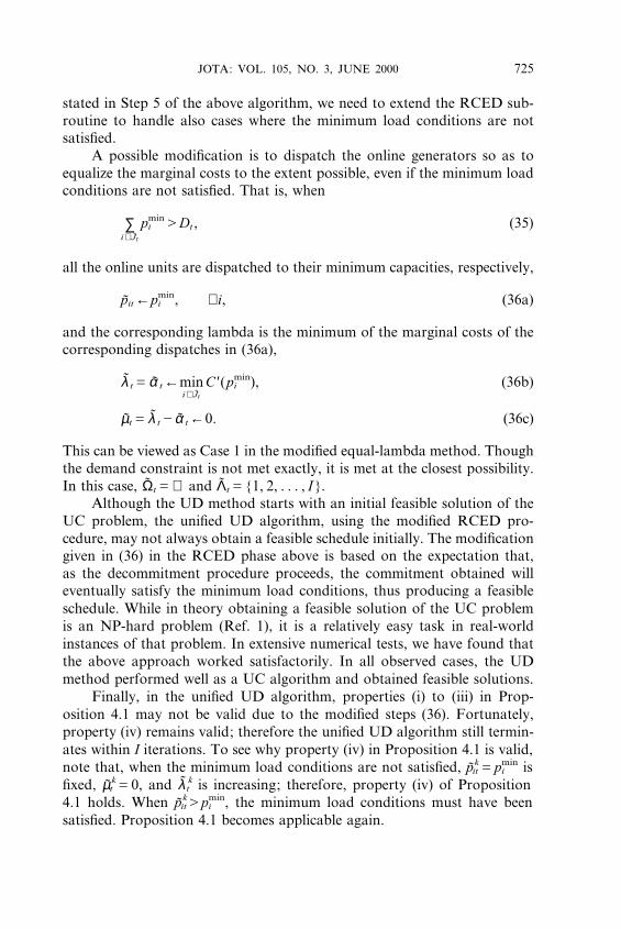
stated in Step 5 of the above algorithm, we need to extend the RCED sub-routine to handle also cases where the minimum load conditions are notsatisfied.

A possible modification is to dispatch the online generators so as toequalize the marginal costs to the extent possible, even if the minimum loadconditions are not satisfied. That is, when

∑i∈Jt

pmini HDt , (35)

all the online units are dispatched to their minimum capacities, respectively,

pit←pmini , ∀i, (36a)

and the corresponding lambda is the minimum of the marginal costs of thecorresponding dispatches in (36a),

λ tGα t←mini∈Jt

C ′(pmini ), (36b)

µtGλ tAα t←0. (36c)

This can be viewed as Case 1 in the modified equal-lambda method. Thoughthe demand constraint is not met exactly, it is met at the closest possibility.In this case, ΩtG∅ and ΛtG1, 2, . . . , I.

Although the UD method starts with an initial feasible solution of theUC problem, the unified UD algorithm, using the modified RCED pro-cedure, may not always obtain a feasible schedule initially. The modificationgiven in (36) in the RCED phase above is based on the expectation that,as the decommitment procedure proceeds, the commitment obtained willeventually satisfy the minimum load conditions, thus producing a feasibleschedule. While in theory obtaining a feasible solution of the UC problemis an NP-hard problem (Ref. 1), it is a relatively easy task in real-worldinstances of that problem. In extensive numerical tests, we have found thatthe above approach worked satisfactorily. In all observed cases, the UDmethod performed well as a UC algorithm and obtained feasible solutions.

Finally, in the unified UD algorithm, properties (i) to (iii) in Prop-osition 4.1 may not be valid due to the modified steps (36). Fortunately,property (iv) remains valid; therefore the unified UD algorithm still termin-ates within I iterations. To see why property (iv) in Proposition 4.1 is valid,note that, when the minimum load conditions are not satisfied, pk

itGpmini is

fixed, µkt G0, and λ k

t is increasing; therefore, property (iv) of Proposition4.1 holds. When pk

itHpmini , the minimum load conditions must have been

satisfied. Proposition 4.1 becomes applicable again.

JOTA: VOL. 105, NO. 3, JUNE 2000726

Theorem 4.2. The unified UD algorithm, with the modification givenin (36) in the RCED phase, terminates within I iterations, where I is thenumber of units.

5. Unit Decommitment vs Lagrangian Relaxation

In this section, we present an intuitive discussion on the relationshipbetween the UD method and the LR method for solving the UC problem.Let λ t and µt, tG1, . . . , T, be the corresponding nonnegative Lagrangemultipliers to (2) and (3). Conventional LR approaches solve the followingdual problem (D):

(D) maxλ ,µX0

d(λ , µ), (37a)

s.t. d(λ , µ) Gminu,p

∑I

iG1∑T

tG1

Ci ( pit)uitCSi (u, t)

C ∑T

tG1

λ t1DtA ∑I

iG1

pituit2C ∑

T

tG1

µt3RtA ∑I

iG1

ri ( pit)uit4G ∑

I

iG1di (λ , µ)C ∑

T

tG1(λ tDtCµtRt ), (37b)

di (λ , µ)Gminuit , pit

∑T

tG1

[Ci ( pit)uitCSi (u, t)

Aλ tpituitAµt ri (pit)uit ]. (37c)

The minimization problem (37c) is subject to (4)–(6) and the initial con-ditions. In (37c), when uitG1, the optimal pit can be obtained by solving

(Qi ) min Ci ( pit)Aλ tpitAµt ri ( pit), (38a)

s.t. pmini YpitYpmax

i . (38b)

Equivalently, this defines a mapping

(λ t , µt) >Qi

pit .

For simplicity, we use pit (λ t , µt ) to denote the mapping. After all subprob-lems di (λ , µ), iG1, . . . , I, are solved, the multipliers λ and µ are thenupdated by the subgradient rule (e.g. Ref. 21) so as to maximize d( · , ·). It

JOTA: VOL. 105, NO. 3, JUNE 2000 727

is well known that, even if (D) is completely solved, it would not yield afeasible schedule.

With pit in (37c) substituted by pit (λ t , µt ), the dual subproblem (37c)can be rewritten as

di (λ , µ)G minuit∈0,1

∑T

tG1

[Ci ( pit (λ t , µt))Aλ tpit (λ t , µt)

Aµt ri ( pit(λ t , µt))]uitCSi (u, t). (39)

Note that di (λ , µ) in (39) is now a 0–1 integer programming problem. Fur-thermore, solving di (λ , µ) in (39) is equivalent to solving the followingproblem:

di (λ , µ)G minuit∈0,1

∑T

tG1

Ci ( pit (λ t , µt))uit

C[λ tpit(λ t , µt)Cµt ri( pit(λ t , µt))](1Auit)CSi (u, t). (40)

To see the equivalence between (39) and (40), add 0 · (1Auit ) to (39), andthen add λ tpit(λ t , µt )Cµt ri ( pit (λ t , µt )) to the payoffs of the decision vari-ables uit and 1Auit , which yields (40).

Solving di (λ , µ), or equivalently solving a unit subproblem di (λ , µ), islike solving a UD problem (23). This implies that a solution of a LR sub-problem is already optimally decommitted in some sense. Given an econ-omically dispatched schedule (u, p, λ , µ) [if u is not dispatchable, use themodified steps (36)], it can be shown that

(λ t , µt ) >Qi

pit .

Starting from this schedule (u, p, λ , µ), performing either the UD step (23)with respect to u or the LR subproblem (37c) with respect to (λ , µ) for anyunit would result in the same (tentative) commitment for that unit. How-ever, at the next iteration, the LR subproblem would consider the tentativecommitments of all units, while the UD method corrects only the commit-ment of one unit (by adopting its tentative commitment). Also, the updatingof the multipliers (λ , µ) is different: UD performs RCED, and LR usessubgradients. The multipliers (λ , µ) obtained from either approach areintended to capture the marginal cost of the demand and reserve constraints,respectively. The unit commitment updating of the LR approaches resultsin overcorrection of the commitments, which leads to its primal infeasibilityat all iterations, while the UD method adjusts the commitment, one unit ata time, toward a feasible commitment and then maintains feasibility there-after. It is fair to say that the UD method is a LR-like method and that theLR approaches perform UD-type operations.

JOTA: VOL. 105, NO. 3, JUNE 2000728

Because of the afore-mentioned primal infeasibility in the dual optimiz-ation, conventional LR approaches fall into a category of two-phase algo-rithms, with a feasibility phase following the first phase of dualoptimization. In Refs. 1 and 16, Tseng et al. suggested to add a third phase,a UD phase, as the postprocessing phase, to the conventional two-phasemethods. This results in a three-phase scheme. The three-phase scheme isreported not only to be able to improve the solution quality, but also tomitigate some unpredictable effect due to heuristics when integrated withthe LR approaches (Ref. 16). Figure 3 gives an illustration of the typicalalgorithm trajectories of the conventional LR two-phase methods, the LRthree-phase method (Refs. 1 and 16), and the proposed unified UDapproach.

6. Numerical Results and Conclusions

We conduct numerical tests to compare the performance of UD andLR. All algorithms are implemented in FORTRAN on an HP 700 work-station. Four cases of systems with combinations of 10 or 30 units and 24or 168 hours of planning horizon are tested. For each case, we generaterandomly 100 instances of the UC problem. Detailed configuration of therandom instances are available upon request to the corresponding author.Each instance is solved by the LR and UD methods. The column under DG

Fig. 3. Illustration of algorithm trajectories.

JOTA: VOL. 105, NO. 3, JUNE 2000 729

Table 1. Comparison of the UD and LR algorithms.

Solution quality CPU timeCaseIBT UD LR DG (%) UD LR

10B24 1.0010 1 0.9 0.2185 1(0.9933–1.10105) (0.09–2.85) (0.1028–0.4773)

10B168 1.0008 1 0.9 0.1500 1(0.9976–1.0054) (0.38–2.04) (0.0978–0.3446)

30B24 1.0013 1 0.28 0.5214 1(0.9981–1.0090) (0.06–0.81) (0.3344–0.8608)

30B168 1.0017 1 0.35 0.2745 1(0.9997–1.0058) (0.15–1.78) (0.1513–0.4152)

(duality gap) records the duality gap of the LR approach in terms of thepercentage of the dual value. Since the comparisons are normalized to thevalue of the LR approach, the columns under LR consist of all ones. Also,the two numbers in parentheses define the range of the sample points. Themean of the sample points is recorded on the top of the correspondingparentheses. The test results including solution qualities and CPU timesrequired for both methods are summarized in Table 1.

From Table 1, we know that the error between LR and UD is within0.2% and that the UD methods take much less (save about 50% at least)CPU time than the LR approach. Besides, the only heuristic in UD is theunit selection rule, which is analogous to choosing a descent direction incontinuous optimization. Our experience indicates that the algorithm per-formance is insensitive to the selection rule. To sum up, the numerical test-ing results show that UD serves as a reliable, efficient, and robust alternativeto the traditional implementations of the LR approaches for solving the UCproblem.

References

1. TSENG, C. L., On Power System Generation Unit Commitment Problems, PhDThesis, University of California at Berkeley, 1996.

2. CHANDLER, W. G., DANDENO, P. L., GILMN, A. F., and KIRCHMAYER, L. K.,Short-Range Operation of a Combined Thermal and Hydroelectric Power System,AIEE Transactions, Vol. 73, No. 3, pp. 1057–1065, 1953.

3. TURGEON, A., Optimal Unit Commitment, IEEE Transactions on AutomaticControl, Vol. 23, No. 2, pp. 223–227, 1977.

4. TURGEON, A., Optimal Scheduling of Thermal Generating Units, IEEE Trans-actions on Automatic Control, Vol. 23, No. 6, pp. 1000–1005, 1978.

JOTA: VOL. 105, NO. 3, JUNE 2000730

5. DILLON, T. S., Integer Programming Approach to the Problem of Optimal UnitCommitment with Probabilistic Reserve Determination, IEEE Transactions onPower Apparatus and Systems, Vol. 97, No. 6, pp. 2154–2164, 1978.

6. PANG, C. K., and CHEN, H. C., Optimal Short-Term Thermal Unit Commitment,IEEE Transactions on Power Apparatus and Systems, Vol. 95, No. 4, pp. 1336–1342, 1976.

7. PANG, C. K., SHEBLE, G. B., and ALBUYEH, F., Evaluation of Dynamic Pro-gramming Based Methods and Multiple Area Representation for Thermal UnitCommitments, IEEE Transactions on Power Apparatus and Systems, Vol. 100,No. 3, pp. 1212–1218, 1981.

8. WOOD, A. J., and WOLLENBERG, B. F., Power Generation, Operation, and Con-trol, John Wiley and Sons, New York, NY, 1984.

9. MUCKSTADT, J. A., and KOENIG, S. A., An Application of Lagrangian Relax-ation to Scheduling in Power-Generation Systems, Operations Research, Vol. 25,No. 3, pp. 387–403, 1977.

10. BERTSEKAS, D. P., LAUER, G. S., SANDELL, N. R., JR., and POSBERGH, T. A.,Optimal Short-Term Scheduling of Large-Scale Power Systems, IEEE Trans-actions on Automatic Control, Vol. 28, No. 1, pp. 1–11, 1983.

11. BARD, J. F., Short-Term Scheduling of Thermal-Electric Generators Using Lag-rangian Relaxation, Operations Research, Vol. 36, No. 5, pp. 756–766, 1988.

12. COHEN, A., and SHERKAT, V., Optimization-Based Methods for OperationsScheduling, Proceedings of IEEE, Vol. 75, No. 12, pp. 1574–1591, 1987.

13. ZHUANG, F., Optimal Generation Unit Commitment in Thermal Electric PowerSystems, PhD Thesis, McGill University, 1988.

14. LEE, F. N., Short-Term Thermal Unit Commitment: A New Method, IEEETransactions on Power Systems, Vol. 3, No. 2, pp. 421–428, 1988.

15. LI, C. A., JOHNSON, R. B., and SVOBODA, A. J., A New Unit CommitmentMethod, IEEE Transactions on Power Systems, Vol. 12, No. 1, pp. 113–119,1997.

16. TSENG, C. L., OREN, S. S., SVOBODA, A. J., and JOHNSON, R. B., A UnitDecommitment Method in Power System Scheduling, Electrical Power andEnergy Systems, Vol. 19, No. 6, pp. 357–365, 1997.

17. IBARAKI, T., and KATOH, N., Resource Allocation Problems: AlgorithmicApproaches, MIT Press, Cambridge, Massachusetts, 1988.

18. BRUCKER, P., An O(n) Algorithm for Quadratic Knapsack Problems, OperationsResearch Letters, Vol. 3, No. 3, pp. 163–166, 1984.

19. SHEBLE, G. B., Real-Time Economic Dispatch and Reserve Allocation UsingMerit Order Loading and Linear Programming Rules, IEEE Transactions onPower Systems, Vol. 4, No. 4, pp. 1414–1420, 1989.

20. STADLIN, W. O., Economic Allocation of Regulating Margin, IEEE Transactionson Power Apparatus and Systems, Vol. 89, No. 4, pp. 1776–1781, 1971.

21. BAZARAA, M. S., SHERALI, H. D., and SHETTY, C. M., Nonlinear Program-ming: Theory and Algorithms, John Wiley and Sons, New York, NY, 1993.