Solving Min-Max Multi-Depot Vehicle Routing Problem∗

John Carlsson†; Dongdong Ge‡; Arjun Subramaniam§;Amy Wu¶; and Yinyu Ye‖

1st May 2007

Abstract

The Multi-Depot Vehicle Routing Problem (MDVRP) is a generalization of theSingle-Depot Vehicle Routing Problem (SDVRP) in which vehicle(s) start from multi-ple depots and return to their depots of origin at the end of their assigned tours. Thetraditional objective in MDVRP is to minimize the sum of all tour lengths, and existingliterature handles this problem with a variety of assumptions and constraints. In thispaper, we explore the notion of minimizing the maximal length of a tour in MDVRP(“min-max MDVRP”). We present two heuristics in the paper. The first heuristic is alinear programming-based approach with global improvement. The second one, the re-gion partition heuristic, is proved to be asymptotically optimal and is potentially usefulfor general network applications. A comparison of the computational implementationsfor different heuristics is presented.

Key words: vehicle routing problem; region partition; heuristic.

1 IntroductionThe Vehicle Routing Problem (VRP) has been one of the central topics in optimization

since Dantzig proposed the problem in 1959 [7]. A simple general model of VRP can bedescribed as follows: a set of service vehicles need to visit all customers in a geographicalregion with the minimum cost.

In the Single-Depot Vehicle Routing Problem (SDVRP), multiple vehicles leave from asingle location (a “depot”) and must return to that location after completing their assignedtours. The Multi-Depot Vehicle Routing Problem (MDVRP) is a generalization of SDVRPin which multiple vehicles start from multiple depots and return to their original depots atthe end of their assigned tours. The traditional objective in MDVRP is to minimize the sum

∗This research is supported in part by the Boeing Company.†Institute of Computational and Mathematical Engineering.‡Department of Management Science and Engineering.§Department of Management Science and Engineering.¶Department of Computer Science.‖Department of Management Science and Engineering and, by courtesy, Electrical Engineering, E–mail:

yinyu-ye@stanford.edu; Stanford University, Stanford, CA 94305, USA.

1

of all tour lengths, and existing literature handles this problem with a variety of assumptionsand constraints.

In this paper, we explore the notion of minimizing the maximal length of a tour in aMDVRP (“min-max MDVRP”) using both theoretical analysis and heuristic design. To thebest of our knowledge, no prior exploration of min-max MDVRP has been published, but thisformulation is advantageous for a number of applications. For example, consider a networkmodel in which depots represent servers and customers represent clients. A network routingtopology generated by solving min-max MDVRP results in a set of daisy-chain networkconfigurations that minimize the maximum latency between a server and client. This canbe advantageous in situations in which the server-client connection cost is high but theclient-client connection cost is low.

The formulation of min-max MDVRP is as follows, with the assumption that all pointsare randomly and uniformly distributed in a Euclidean plane:

minimize λsubject to TSP (Si) ≤ λ, ∀i

∪Si = N ,

where N is the set of all customers, Si(⊂ N ) is the subset of customers assigned to vehiclei, and TSP (S) is the minimal TSP tour length that visits all customers in set S.

The implementation results demonstrate the efficiency of the heuristic methods devel-oped in this paper, as they reduce MDVRP to a sequence of smaller-scale TSP problems inpolynomial time. In addition, the sum of all tour lengths that our methods generate is highlycomparable to the minimized total lengths produced by traditional approaches. And thesemethods are also capable of quickly processing tens of thousands of customers, a scalabilityproperty which is becoming increasingly important as networks expand in size.

In this paper we first give a theoretical analysis for the optimal solution of min-maxMDVRP by developing lower and upper bounds. We show that the optimal solution tomin-max MDVRP is asymptotically close to the optimal TSP tour of all customers dividedby the number of depots when the ratio of customers to depots is high. The same conclusionapplies to the solution generated by a region partition algorithm when the number of depotsis fixed.

Then we develop two heuristics to min-max MDVRP. The first heuristic is a linearprogramming-based heuristic with a global load balancing technique. By starting from asimple linear programming-based algorithm, we rapidly assign customers to depots and gen-erate TSP routes for each vehicle. The solution is further improved in a post refinementperiod in which we keep changing certain parameters globally. Next, noticing that a convexequitable region partition yields an even division of points (i.e., if we divide the service regioninto a set of subregions with equal area, then each subregion will contain – asymptotically– the same number of points), we propose a fast approximation algorithm to generate goodinitial solutions for min-max MDVRP. The solution can then be improved with common localimprovement procedures. Moreover, this region partition method, for which we demonstrateboth theory and implementation, is potentially useful in many network design problemswith regular topology structures, such as the Steiner tree and the minimum spanning forestproblem.

2

The simulation results of these two methods and a routine heuristic are compared andanalyzed in the performance analysis section. Finally, we summarize our results and addressfuture research issues.

2 Asymptotic Bounds on Min-Max MDVRP

2.1 Analysis of Optimal Solutions

Since the MDVRP is NP-hard, researchers have made compelling efforts to design heuris-tics; in addition, exploring the theoretical bounds of this problem has been an intriguing topicas well. Baltz et al. proved that the sum of all tour lengths asymptotically approaches αkn

d−1d

with the uniform distribution, and αk depends on the number of depots. In this section,we provide lower and upper bounds for min-max MDVRP in a planar graph and prove itsasymptotic convergence for a broad class as the problem size expands. To provide context,we will first review known results for the probabilistic TSP. The most celebrated discoveryis the BHH theorem (1959) by Beardwood, Halton and Hammersley.

Theorem 1. (BHH Theorem) Suppose Xi’s, 1 ≤ i ≤ n, are independent and identicallydistributed random points uniformly distributed in a unit cube [0, 1]d, d ≥ 2. Then withprobability one, the length TSP (X1, X2, · · ·Xn) of an optimal TSP tour traversing allpoints satisfies:

limn→∞

TSP (X1, X2, · · · , Xn)/n d−1d = α(d),

where α(d) is a positive constant depending on d.

Considering that we are only interested in planar graphs, we assume all customers anddepots are uniformly and randomly distributed in a unit square, and define α ≡ α(2) inour discussion. Denote the set of depots by D = D1, D2, · · · , Dm, |D| = m. Denotethe set of vehicles by V = V1, V2, · · · , Vk, |V| = k ≥ m. In the case k = m, we alwaysassume each depot has one single vehicle. Denote the set of nodes(or customers) by N =N1, N2, · · · , Nn, |N | = n. We will use node and customer interchangeably in this paper.Denote the value of an optimal solution to min-max MDVRP by L, i.e., L is the lengthof the longest tour. Denote the largest distance between an arbitrary pair of points in twodifferent sets A and B by d(A,B), i.e., d(A,B) = max

x∈A,y∈B||x− y||.

First we have the following observation:

Lemma 2. For a general planar graph (points do not necessarily follow any distribution),

TSP (D ∪N )− TSP (D)

k≤ L ≤ TSP (N )

k+ 2 ∗ d(D,N ).

Proof. Consider the lower bound first.In an optimal pattern of min-max MDVRP, assume the sum of all tour lengths is Sopt.

Note that L is the longest tour, we have

k ∗ L ≥ Sopt.

3

Add an optimal TSP tour T for all the depots to this pattern. Now each point(node ordepot) in the graph has an even degree, which implies an Euler tour. This Euler tour canbe reduced to a feasible TSP tour for the set of all the depots and nodes. Then,

Sopt + TSP (D) ≥ TSP (D ∪N ).

Therefore,

L ≥ TSP (D ∪N )− TSP (D)

k.

For the upper bound, consider a tour partition heuristic.

Heuristic 1 Tour Partition Heuristic1. Generate an optimal TSP tour for all the nodes.

2. Partition this tour into k equal subtours t1, t2, · · · , tk.3. Connect both the starting and ending nodes of subtour ti to the depot where vehicle

i stays.

This heuristic generates a feasible solution for the MDVRP. The maximal tour length,which is an upper bound of L, is at most

TSP (N )

k+ 2 ∗ d(D,N ).

The proof implies that the lower bound holds even when L is the average length of allthe tours, so it is not tight. However, when the ratio of nodes to depots is high, we canderive the asymptotic bounds for L.

Corollary 3. (a) When k = o(√

n),

limn→∞

L√n/k

= α.

(b) For non-fixed MDVRP, i.e., a vehicle can start from and return to arbitrary differentdepots, if n = Ω(k log2 k) and k = m,

limn→∞

L√n/k

≤ α.

Proof. (a) According to the BHH theorem, for arbitrarily small ε, when n,m are sufficientlylarge,

α((1− ε)√

m + n− (1 + ε)√

m)

k≤ L ≤ α(1 + ε)

√n

k+ 2d(D,N ) + ε. (1)

4

Noticing that m ≤ k and k = o(√

n), we know√

m/k is less than 1, while√

m+nk

goesto infinity as n goes to infinity. On the other side, d(D,N ) is bounded by a constant while√

n/k goes to infinity as n goes to infinity.(b) Consider the tour partition heuristic. Then at Step 3 in Heuristic 1, for each subtour

ti, instead of connecting its starting and ending nodes to the depot where vehicle i stays,we consider a perfect matching between depots and starting points of subtours, and anotherperfect matching between depots and ending points of subtours.

The min-max perfect matching for uniformly distributed points has the bound providedby Leighton and Shor in 1989 [13]: if Xi’s and Yi’s are independent and uniformly distributedpoints on a unit square for 1 ≤ i ≤ r, then there exists a constant C, such that

minσ∈P

max1≤i≤r

||Xi − Yσ(i)|| ≤ Cr−12 (log r)

34 (2)

with probability one as r →∞, where P is the set of all permutations of 1, 2, · · · , r.First apply the bound (2) to depots and all starting points of subtours. Then apply it

again to depots and all ending points of subtours. We get L ≤ α(1+ε)√

nk

+ 2Ck−12 (log k)

34 .

With the assumption n = Ω(k log2 k), we complete the proof.

For the general case k = λn+ o(n), λ ≥ 0, Baltz et al. [3] proved that the sum of all tourlengths asymptotically approaches α′

√n as n → ∞, where the constant α′ is equal to the

TSP constant α for the case λ = 0 and depends on λ for the case λ > 0. Therefore, we canobtain a direct lower bound according to their results.

Lemma 4. When k = λn + o(n), λ ≥ 0,

limn→∞

L√n/k

≥ α′,

where the constant α′ is defined as above.

2.2 Bounds by Region Partition Heuristics

Based on the discussion above, we can conclude that the optimal solution to min-maxMDVRP with uniform distributed points will numerically approach α

√n/k, the value of

the optimal TSP tour of all customers split by the number of vehicles, under the constraintk = o(

√n). This matches our intuition, although the constraint is restrictive. We would like

to relax this constraint to a broader class and derive some nontrivial bounds by analyzinglocal performance in large size problems. In this section, we will analyze a region partitionheuristic with theoretically good performances, and an estimation on upper bounds for allcases k = Ω(

√n) derived from a grid region partition.

Before presenting the heuristics, we need several lemmas to review some facts:

Theorem 5. (Convex Region Partition Theorem) Given k points in a convex bounded planarpolygon, it is always possible to find a partition of the domain into k equal-area convexpolygons, with exactly one point in each face.

5

This convex region partition theorem was proved in [4] for both continuous and discreteversions, and an algorithm for discrete version was also given. An algorithm for the contin-uous version, i.e. the convex region partition described in the theorem was recently revealedby Carlsson and Armbruster [1].

For the time being, we assume an equitable partition exists and develop a theoreticalrationale for the desirability of such a partition. The next two lemmas will prepare us someimportant backgrounds for analyzing region partition approaches.

Lemma 6. (Occupancy Lemma) Randomly put n balls into m bins with equal probability. Ifn = Ω(m log2 m), then the number of balls in the bin holding the least balls has an asymptoticperformance as n

m. So does the number of balls in the bin holding the most balls.

Proof. This fact can be proved by Chernoff bounds. We will give a sketch of the proof here.We only consider the case n = m log2 m here. For an arbitrary bin, define xi is 1 if the

ith ball falls into this bin, and 0 otherwise. Let Si = x1 + x2 + · · · + xi. Note that theexpected number of balls falling into a bin is log2 m. From the Chernoff bounds [12],

P = Prob(Sn ≤ n

m(1− 2

√2

log m)) ≤ e−nD(p−px||p),

where p = 1m, x = 2

√2

log m, D(a||b) = a log a

b+ (1− a) log 1−a

1−b.

When m is sufficiently large, we have

e−nD(p−px||p) ≤ e−n(px2/4) =1

m2.

Therefore, the probability that one bin has less than nm

(1 − 2√

2log m

) balls is at most

mP ≤ 1m.

Similarly, by applying another Chernoff bound, we can also prove that the probabilitythat one bin has more than n

m(1 + 2

√2

log m) balls is at most 1

m.

Simple scaling arguments show that the BHH theorem still holds even if the unit cube isreplaced by an arbitrary compact subset K in Rd in [18]. This fact suggests that the limitis independent of the shape of the compact set K.

Theorem 7. (generalized BHH Theorem [18]) In particular, if for i ≥ 1, Xi’s are i.i.d withuniform distribution on a compact set K of Lebesgue measure one, the BHH theorem stillholds.

We consider a region partition heuristic for min-max MDVRP for the case k = m.

Heuristic 2 Region Partition Heuristic1. Divide the region into k equitable convex polygons such that each polygon has exactly

one vehicle inside.

2. Find an optimal TSP tour for each vehicle and the nodes in the same subregion.

With the fixed number of depots, we have

6

Figure 1: The perturbation method, and its subsequent effects on assignment and routesgeneration. Here the routes are suggested by arrows emanating from each depot node.

Lemma 8. If k=O(1), the solution L generated by Heuristic 2 satisfies:

limn→∞

L√n/k

= α.

Proof. Assume the region with the most nodes has Nmax = n/k + t nodes. From Occupancy

lemma, we know limn→∞

t

n/k= 0. Therefore, from the generalized BHH theorem, we know:

L ≤ α(1 + o(1))√

Nmax

√1

k≤ α(1 + o(1))

√(1 + o(1))

n

k

√1

k≤ α(1 + o(1))

√n

k.

On the other hand, since the region with the most nodes has at least n/k nodes, theclaim is true:

limn→∞

L√n/k

= α.

The lemma implies that the length of the longest tour generated by the region partitionheuristic is asymptotically close to a lower bound when the size of the problem expands.Thus this heuristic is asymptotically optimal in this case.

If vehicles are more than depots available (k > m), we can use the perturbing idea togenerate their routes. In this procedure, if there are two or more vehicles on the same depot,we only need to slightly relocate vehicles evenly distributed on a small circle encircling thatdepot (Figure 1). For a sufficiently small perturbation, the algorithm remains feasible, andthe optimal value only changes marginally.

If the ratio of n to k is smaller, for example, n = O(k log k), it is harder to predict theoptimal solution. Motivated by the Occupancy lemma, we still can derive an asymptoticupper bound. The following theorem illustrates an extreme case:

Theorem 9. Assume k = m, i.e., all vehicles are i.i.d. in the square. If the number ofvehicles is proportional to the number of nodes, i.e., k = λn, 0 < λ < 1, then with probabilityone, as k →∞,

L ≤ (α

λ+ 2

√2 log n)

1√n

.

7

Proof. We divide the unit square into n/ log2 n smaller squares each of which has the sidelength log n/

√n. Then, from the Occupancy lemma, we know that any small square has

at most log2 n + O(log n) nodes and at least λ(log2 n − O(log n)) vehicles with probabilityone as n → ∞. Apply the tour partition heuristic to the square with the most customers.According to the generalized BHH theorem and Lemma 2, we have

L ≤α√

log2 n + O(log n)

λ(log2 n + O(log n))

log n√n

+ 2√

2log n√

n≈ (

α

λ+ 2

√2 log n)

1√n

.

Applying the similar argument, we obtain an upper bound for the case k = Ω(√

n):

Corollary 10. Assume all vehicles are uniformly distributed in the cube and k = Ω(√

n),then with high probability, as k →∞,

L ≤ α√

n

k+ 2

√2log k√

k.

3 An LP-based Load Balancing HeuristicWe present a linear programming-based heuristic in this section, which uses a global load

balancing technique during post-refinement periods.Although many heuristics have been applied to solve the SDVRP and MDVRP, we are

unaware of any existing specific heuristic or theoretical results for min-max MDVRP, espe-cially in the large-size case. In general literature, one idea to solve the MDVRP is a two-stageheuristic(for example: Wren and Holliday [17]): construct an initial solution, then apply anumber of local improvements. The initial solutions in common heuristics are usually con-structed by the nearest neighbor assignment. Gillet and Johnson [9] proposed a clusteringheuristic which used a sweep heuristic at each depot. Golden et al. [11] presented two heuris-tics for MDVRP; the second one specifically solved the large-size problem by a two-stagealgorithm which assigns nodes to depots first and then built TSP tours for each vehicle. Chaoet al. [5] proposed a simple initialization heuristic followed by a refinement, which gainedthe best performance in many benchmark problems. In 2002, Giosa et al. [10] demonstrateda series of 2-stage heuristics to solve MDVRPTW. Recently, Lim and Wang [14] gave aone-stage approach to MDVRP with the constraint each depot only has a fixed number ofvehicles. Baltz et al. [2, 3] presented a probabilistic analysis of the optimal solution for theproblem. Tansini [16] proposed a polynomial-time approximation scheme (PTAS) for theMDVRP similar to Arora’s PTAS algorithm for TSP.

Our heuristic is based on a load balancing idea: the load for each vehicle must be almostbalanced in an optimal plan, so each vehicle is assigned the same working load in terms ofthe number of nodes to serve. This intuition is plausible considering that the distribution ofnodes in our model is uniform. We carefully balance the number of nodes assigned to eachdepot by linear programming at the first step, then generate a near-optimal route for eachvehicle by using the Concorde TSP solver [6]. The solution is further improved by global

8

0 10 20 30 40 50 60 70 80 90 1000

10

20

30

40

50

60

70

80

90

100

0 10 20 30 40 50 60 70 80 90 1000

10

20

30

40

50

60

70

80

90

100

0 10 20 30 40 50 60 70 80 90 1000

10

20

30

40

50

60

70

80

90

100

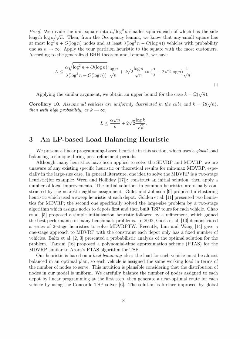
Figure 2: The initial input (a), the assignment (b), and the final construction of TSP tours(c).

adjustment of the number of nodes assigned to vehicles, rather than traditional local searchprocedures.

Assume all customers are uniformly distributed on a square and the locations of depotsare randomly distributed. A depot is allowed to have more than one vehicle. Each vehiclemust return to the depot from which it originates. First we assume that each depot hasexactly one vehicle, and no two depots share a location (this assumption will be generalizedlater). Suppose each node Xj, 1 ≤ j ≤ n, is located at (xj, yj), and each vehicle Vi, 1 ≤ i ≤ k,is located at (vi, wi). The distance cij between Xj and Vi is ||(xj, yj)− (vi, wi)||.

Define xij to be a binary variable indicating if node Xj is assigned to vehicle Vi or not.We build an integer program for clustering:

(LP ) : minimize∑

1≤i≤k,1≤j≤n

cijxij

subject to∑

1≤j≤n

xij =n

k, ∀i,

∑

1≤i≤k

xij = 1, ∀j,

xij ∈ 0, 1, ∀i, j,

where we assume that n/k is an integer(the fractional case will be discussed later).Note that its linear program relaxation (LPR) is a typical network flow model, so any

vertex solution to LPR will be integral. Therefore, we can directly solve LPR for the initialassignment.

A sketch of the heuristic is as follows:

9

Heuristic 3 LP-based Load Balancing Heuristic1. Build LPR and solve it.

2. Build a TSP tour for each vehicle by the Concorde solver. Assume that their lengthsare sorted in a descending order L1, · · · , Lk.

3. If (L1 − Lk)/Lk ≤ r, with r a small constant, or if the linear program has been runmany times, stop and output a current best solution. Otherwise, decrease the numberof nodes assigned to vehicles having longer tours and increase the number of nodesassigned to vehicles having shorter tours (we will explain details later). This way, anew revised LP is generated. Return to step 1 and repeat the procedure.

A sketch of the heuristic in one loop is shown in figure 2.There are several details we need to explain in our algorithm.Note 1: If n/k is fractional. Assume n = pk+q. p and q are integers and q is the residue.

Then we assign the first q vehicles p + 1 nodes and assign each of the remaining vehicles pnodes. Thus the number of nodes assigned to each vehicle is always an integer.

Note 2: Constant r in step 3 is a ratio threshold to measure the output, which can beadjusted according to the need for accuracy. In most cases, setting r = 25% is enough toachieve a satisfactory result.

Note 3: At step 3, if (L1−LK)/LK ≤ r, we adjust the number of nodes assigned to eachdepot by the following procedure:

• Build the sets L+ = i : Li− L > 0, L− = i : Li− L < 0, where L is the average oftour length.

• Without loss of generality, assume s = |L+| ≥ |L−|. For any i ∈ L+, define the relativedrift d+

i = Li−LL

. Decrease the number of nodes assigned to depot i by [c ∗ di

r](c is a

constant empirically decided. We set c = 2 in implementation). Sort elements in L−

in the descending order of their tour lengths. Then define d−i = L−Li

Lfor the first s

elements in L−. Increase the number of nodes in the same way.

• If the number of nodes removed from L+ is more than the number of nodes added toL−, add one node to each element in L− sequentially starting from the depot whichhas the fewest nodes, keep doing that until nodes are balanced. Repeat the similarprocedure for the contrary case.

3.1 Multiple Vehicles on a Depot

We have assumed that each depot includes exactly one vehicle in all the heuristics afore-mentioned. However, in a practical situation, multiple vehicles may lie on the same depot.We need to extend our heuristics to this general case. If we still follow the original pro-cedures and assign the same number of nodes to each vehicle instead of each depot, thesolution is poor, because nodes are assigned to each such vehicle randomly – therefore, ourinitial geometric intuition for node assignment is lost (Figure 3).

10

0 10 20 30 40 50 60 70 80 90 1000

10

20

30

40

50

60

70

80

90

100

0 10 20 30 40 50 60 70 80 90 1000

10

20

30

40

50

60

70

80

90

100

0 10 20 30 40 50 60 70 80 90 1000

10

20

30

40

50

60

70

80

90

100

Figure 3: Problems encountered when multiple vehicles are assigned to a single depot. (a) isthe initial node set given to the problem (we have 8 vehicles and 4 depots) and (b) representsa solution without the perturbation applied. (c) represents a solution with the perturbationapplied; it is clearly preferable, as vehicle routes do not intersect.

In order to work around this difficulty for vehicles in a same depot, we perturb thelocations of vehicles located at the same depot before generating cij’s. Each vehicle isrelocated to a new location lying in a small circle around that depot, keeping them evenlydistributed on that circle. This small change will dramatically improve the final solution(Figure 1). We can generate good solutions with this technique.

4 A Region Partition HeuristicThe second heuristic we present is the region partition heuristic (Heuristic 2) based on

the algorithm in [1] that takes as input a convex planar region C and a set of m depotsD = D1, . . . , Dm, and outputs a partition of C into m convex subregions satisfying thefollowing properties:

• Each subregion is convex.

• Each subregion contains one depot Di.

• Each subregion has equal area.

Note that a Voronoi diagram satisfies the first two properties, but not the third. An exampleof such a partition is shown in figure 4.

As mentioned previously, the requirement that each subregion have equal area ensuresthat the lengths of the TSP tours of each region be equal asymptotically [18]. This resultapplies to any compact subset of R2 with Lebesgue measure one, but we require that theseregions be convex for practical purposes. The shortest path between any two cities in asubregion Ri is a straight line, and we want to ensure that the route taken from these onecity to the next lie in the same service region and therefore be feasible.

Many network structures, like minimum spanning trees and Voronoi graphs, have conclu-sions similar to that of the travelling salesman tour, i.e., their lengths converge asymptoticallyin a manner similar to the BHH theorem. For example, [19] describes a similar result forMinimum Spanning Tree (MST). Region partition is therefore a potentially powerful tool not

11

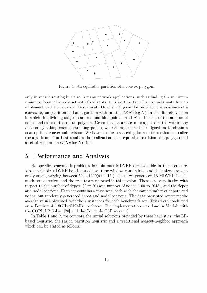
Figure 4: An equitable partition of a convex polygon.

only in vehicle routing but also in many network applications, such as finding the minimumspanning forest of a node set with fixed roots. It is worth extra effort to investigate how toimplement partition quickly. Bespamyatnikh et al. [4] gave the proof for the existence of aconvex region partition and an algorithm with runtime O(N

43 log N) for the discrete version

in which the dividing subjects are red and blue points. And N is the sum of the number ofnodes and sides of the initial polygon. Given that an area can be approximated within anyε factor by taking enough sampling points, we can implement their algorithm to obtain anear-optimal convex subdivision. We have also been searching for a quick method to realizethe algorithm. Our best result is the realization of an equitable partition of a polygon anda set of n points in O(Nn log N) time.

5 Performance and AnalysisNo specific benchmark problems for min-max MDVRP are available in the literature.

Most available MDVRP benchmarks have time window constraints, and their sizes are gen-erally small, varying between 50 ∼ 1000(see [15]). Thus, we generated 13 MDVRP bench-mark sets ourselves and the results are reported in this section. These sets vary in size withrespect to the number of depots (2 to 20) and number of nodes (100 to 2048), and the depotand node locations. Each set contains 4 instances, each with the same number of depots andnodes, but randomly generated depot and node locations. The data presented represent theaverage values obtained over the 4 instances for each benchmark set. Tests were conductedon a Pentium 4 1.8GHz/512MB notebook. The implementation was done in Matlab withthe COPL LP Solver [20] and the Concorde TSP solver [6].

In Table 1 and 2, we compare the initial solutions provided by three heuristics: the LP-based heuristic, the region partition heuristic and a traditional nearest-neighbor approachwhich can be stated as follows:

12

Heuristic 4 Nearest Neighbor Heuristic1. Assign each node to its nearest depot.

2. Build a TSP route for each vehicle accordingly; get an initial solution for the problem.

3. Run the local improvement method to improve the solution.

We have also implemented a modified version of a local improvement procedure proposedby Chao et al. [5] called “1-point movement”. In Table 3 and 4, we present the final outputs offour heuristics. The first heuristic uses the LP-based load balancing heuristic ( Heuristic 3) todistribute the load evenly among vehicles. The other three heuristics all use the modified 1-point movement improvement method in their post optimization periods although they startwith different initial assignments. The second heuristic uses the same initial assignment asthe first heuristic. The third heuristic starts with the region partition method, and the lastone starts with the nearest neighbor assignment.

We have applied different heuristics on each instance and presented in the tables thevalue of the longest tour(“Max”), the value of the shortest tour(“Min”), the average valueof all tours(“Mean”) and the CPU time(“Time”). The primary goal of these heuristics is tominimize the value of the longest tour. The running time of the LP-based load balancingheuristic is primarily comprised of the execution time of the LP and TSP solvers. Therunning time of the region partition with local improvement method (Heuristic 2) mainlyconsists of the running time of the region partition heuristic and TSP solvers. For small tomedium-sized benchmarks, the main bottleneck for all heuristics is finding a near optimalTSP tour for each depot using the Concorde solver.

We have made the following observations based on the simulation results presented inthe tables.

First, according to Table 1 and 2, both LP-based and region partition heuristics pro-duce notably better initial routes than the traditional nearest neighbor approach. They areefficient and effective candidates for the initial assignment.

Second, the region partition heuristic with local improvement produced the best solu-tions(“Max”) for 7 out of 13 instances, and the LP-based load balancing heuristic generatedthe best solutions for 5 out of 13 instances. They both maintained a competitive runningtime, as seen in Table 3 and 4.

Third, when the number of depots is small, the region partition heuristic tends to out-perform the other three heuristics, and its running time remains low. The LP-based loadbalancing heuristic performs better as the number of depots is increased.

Fourth, the region partition heuristic with local improvement and the LP-based loadbalancing heuristic not only improve the maximal tour length as compared to the initialsolution, but they also do not significantly increase the sum of all tour lengths, suggestingthat the adjustment will not lead to a major global increase in cost.

Finally the region partition heuristic with local improvement generates a higher totalcost than the LP-based load balancing heuristic in most instances, though it obtains thebest results for min-max MDVRP in more instances than the latter. This fact demonstratesthat the difference of objective functions between usual MDVRP and min-max MDVRP

13

Table 1: Summary of First Iteration Solutions for Three Heuristics

LP-TSP Region PartitionDataset Depots Nodes Max Min Mean Time Max Min Mean Timed2n100 2 100 472.61 391.12 431.87 1.07 429.22 399.90 414.56 1.10d2n500 2 500 870.76 847.10 858.93 41.70 875.66 843.35 861.00 28.34d5n100 5 100 242.12 159.50 197.15 1.13 209.24 162.26 190.24 2.20d5n500 5 500 378.95 332.04 356.64 6.43 377.97 334.34 356.03 9.06d5n1000 5 1000 542.37 467.60 503.22 35.65 522.34 473.58 497.20 36.73d10n1000 10 1000 283.32 225.20 252.86 11.03 277.63 233.97 255.43 41.11d10n2000 10 2000 380.10 331.38 355.08 115.34 378.11 317.47 353.58 180.76d16n256 16 256 161.22 75.21 106.87 12.16 140.74 70.26 105.51 21.47d16n512 16 512 182.11 106.46 132.74 10.95 172.55 106.58 131.59 22.32d16n1024 16 1024 206.95 149.55 173.64 17.31 196.16 145.83 169.19 57.66d16n2048 16 2048 263.61 207.90 231.87 91.03 253.85 206.56 229.62 230.51d20n1000 20 1000 172.29 117.07 139.24 24.95 170.34 118.31 138.16 84.88d20n2000 20 2000 207.23 167.49 184.83 83.02 222.11 160.57 185.62 177.91

Table 2: Continued: Summary of First Iteration Solutions for Three Heuristics

Nearest NeighborDataset Depots Nodes Max Min Mean Timed2n100 2 100 574.85 260.88 417.85 0.35d2n500 2 500 1097.33 715.18 906.25 48.33d5n100 5 100 268.58 95.23 186.30 0.20d5n500 5 500 519.58 223.48 369.35 5.00d5n1000 5 1000 1101.95 163.28 511.98 295.65d10n1000 10 1000 451.18 83.50 257.03 11.68d10n2000 10 2000 688.58 178.15 361.55 351.40d16n256 16 256 186.23 23.03 91.40 1.38d16n512 16 512 265.48 32.13 122.93 2.33d16n1024 16 1024 419.10 50.58 167.35 12.55d16n2048 16 2048 496.25 72.25 230.63 243.13d20n1000 20 1000 278.38 36.50 134.63 8.75d20n2000 20 2000 368.88 57.25 183.35 49.10

14

Table 3: Summary for Improved Heuristics

LP-TSP + Load Balancing LP-TSP + Local ImprovementDataset Depots Nodes Max Min Mean Time Max Min Mean Timed2n100 2 100 458.35 403.23 430.80 9.18 448.93 443.28 446.10 6.65d2n500 2 500 868.60 846.50 859.53 192.35 865.00 863.63 864.33 187.33d5n100 5 100 207.08 172.08 190.58 8.85 229.45 174.68 215.50 7.83d5n500 5 500 377.28 332.20 357.08 57.90 374.65 357.33 368.03 60.85d5n1000 5 1000 531.85 467.73 501.05 192.58 534.73 488.08 520.13 202.33d10n1000 10 1000 277.83 229.28 252.93 84.88 279.90 224.80 262.23 86.10d10n2000 10 2000 378.65 331.60 355.43 875.45 379.70 335.68 365.88 1098.43d16n256 16 256 114.63 88.08 101.98 68.60 142.63 75.55 112.75 61.23d16n512 16 512 142.15 118.70 131.55 78.75 171.95 108.08 144.38 73.60d16n1024 16 1024 187.98 155.00 171.98 153.88 201.05 150.58 178.10 134.05d16n2048 16 2048 254.75 209.05 231.55 870.18 261.83 207.18 235.10 860.70d20n1000 20 1000 151.05 124.20 138.20 192.15 166.33 117.25 145.65 166.93d20n2000 20 2000 201.43 168.25 184.80 601.60 205.03 168.75 189.13 612.70

Table 4: Continued: Summary for Improved Heuristics

Region Partition+Local Imp Nearest Neighbor+Local ImpDataset Depots Nodes Max Min Mean Time Max Min Mean Timed2n100 2 100 416.70 414.03 415.38 5.73 528.75 313.88 421.30 6.60d2n500 2 500 873.15 869.18 871.15 152.38 913.35 851.85 882.60 135.03d5n100 5 100 204.80 187.00 199.40 8.98 235.20 141.35 204.73 7.58d5n500 5 500 371.88 339.00 359.00 62.18 447.48 261.73 381.85 72.90d5n1000 5 1000 518.33 499.83 511.43 247.50 858.75 253.08 548.78 321.43d10n1000 10 1000 270.50 238.30 260.30 165.03 391.08 124.85 282.80 150.03d10n2000 10 2000 375.50 335.80 363.25 923.58 574.48 173.93 362.43 1206.25d16n256 16 256 132.33 80.08 111.85 74.18 156.93 23.68 102.60 58.80d16n512 16 512 168.15 106.93 143.68 75.03 204.70 35.38 136.63 64.08d16n1024 16 1024 191.68 151.65 176.75 182.20 321.70 57.45 184.38 188.48d16n2048 16 2048 250.95 207.40 233.63 1062.70 414.53 90.43 238.30 1011.68d20n1000 20 1000 163.70 118.13 143.43 229.15 244.88 41.20 144.58 242.35d20n2000 20 2000 219.38 162.65 191.60 543.58 335.48 59.93 209.18 617.83

15

motivates different types of algorithms.

6 ConclusionThis paper has presented the first study to min-max MDVRP. We explored some the-

oretical asymptotic properties of the optimal solution, which gave rise to the region parti-tion heuristic. The region partition idea may have applications beyond the vehicle routingproblem. An LP-based heuristic with global improvement was also presented to solve verylarge-sized problems effectively. We concluded by reporting our simulation results.

Many interesting topics remain after this first attempt in min-max MDVRP. For example,from a theoretical point of view, accurate estimation of the optimal solution in large-scaleproblems for the general case is still open. Our theoretical and implemented work can serveas starting points for further exploration as well.

The techniques used in our algorithms provide advantages over traditional local searchmethods. For example, since the LP-based load balancing heuristic does not inherentlyrequire that the points be scattered in a Euclidean space, it can be adapted as a backendto existing map software to solve VRPs with actual geographic locations. In addition, theregion partition algorithm can be applied to problems outside the scope of VRP. An exactconvex region partition algorithm will be helpful not only for high-quality initial solutionsto MDVRPs, but also for solving a class of network problems with similar structures and amin-max objective function.

References[1] B. Armbruster, J. Carlsson. Finding equitable convex partitions of points in a polygon

efficiently. Submitted for publication, 2006.

[2] A. Baltz, D. P. Dubhashi, A. Srivastav, L. Tansini, S. Werth. Probabilistic Analysis fora Multiple Depot Vehicle Routing Problem. Foundations of Software Technology andTheoretical Computer Science, 25th International Conference(FSTTCS), pp 360-371,2005

[3] A. Baltz, D. P. Dubhashi, A. Srivastav, L. Tansini, S. Werth. Probabilistic Analysisfor a Multiple Depot Vehicle Routing Problem. Random Structure and Algorithms, pp206-225, 2007.

[4] S. N. Bespamyatnikh, D. G. Kirkpatrick, J. Snoeyink. Generalizing Ham Sandwich Cutsto Equitable Subdivisions. Symposium on Computational Geometry (SoCG), pp 49-58,1999.

[5] I.-M. Chao, B. Golden, E. Wasil. A new heuristic for the multidepot vehicle routingproblem that improves upon best-known solutions. American Journal mathematicalmanagement Science, Vol. 13, No 3, pp 371-406, 1993.

[6] W. Cook, Concorde solver for the TSP, Version 1.1. Computer software.http://www.tsp.gatech.edu/concorde.html

16

[7] G.B. Dantzig, J.H. Ramser. The truck dispatching problem. Management Science, Vol.6:60, 1959.

[8] J.F. Soumis, M. Desrochers A New Optimization Algorithm for the Vehicle Rout-ing Problem With Time Windows by Column generation. Networks, Vol. 14, pp 545-565,1984

[9] B. Gillet, J. Johnson Multi-terminal vehicle-dispatching algorithm. Omega, Vol. 4, pp711-718, 1976.

[10] I. Giosa, I. Tansini, I. Viera. New assignment algorithm for the multi-depot vehiclerouting problem. Journal of Operations Research Society, Vol. 53, pp 283-292, 1984.

[11] B.L. Golden, EL. Magnanti, H.Q. Nguyen. Implementing vehicle routing algorithms.Networks, Vol. 7, pp 113-148, 1977.

[12] W. Hoeffding. Probability inequalities for sums of bounded random variables. Journalof the American Statistical Association. 58 (301): 13-30, Mar. 1963.

[13] T. Leighton, P.W. Shor. Tight Bounds for minimax grid matching with applications tothe average case analysis of algorithms. Combinatorica, Vol. 9, pp 161-187, 1989

[14] A. Lim, F. Wang Multi-Depot Routing Problems: A one-Stage Approach. IEEE trans-actions on automation science and engineering, Vol. 2, No. 4, Oct. 2005.

[15] http://www.top.sintef.no/vrp/benchmarks.html

[16] L. Tansini. Department of Computer Science, Chalmers Univeristy, PhD Thesis. Toappear.

[17] A. Wren, A. Holliday. Computer scheduling of vehicles from one or more depots to anumber of delivery points. Operations Research Quarterly, Vol. 23, pp 333-344, 1972.

[18] J. E. Yukich. Probability Theory of Classical Euclidean Optimization Problems. LectureNotes in Mathematics, Vol. 1675, 1998.

[19] J. M. Steele. Growth rates of Euclidean minimal spanning trees with power weightededges. Annals of Probability, Vol. 16, pp 1767-1787, 1988.

[20] X. Zhang, Y. Ye. COPL Computational Programming Optimization Library : LinearProgramming. Computer software. http://www.stanford.edu/ yyye/Col.html

17