some classical problems in random geometry

HAL Id: hal-02377523https://hal.archives-ouvertes.fr/hal-02377523

Submitted on 23 Nov 2019

HAL is a multi-disciplinary open accessarchive for the deposit and dissemination of sci-entific research documents, whether they are pub-lished or not. The documents may come fromteaching and research institutions in France orabroad, or from public or private research centers.

L’archive ouverte pluridisciplinaire HAL, estdestinée au dépôt et à la diffusion de documentsscientifiques de niveau recherche, publiés ou non,émanant des établissements d’enseignement et derecherche français ou étrangers, des laboratoirespublics ou privés.

Some Classical Problems in Random GeometryPierre Calka

To cite this version:Pierre Calka. Some Classical Problems in Random Geometry. Stochastic geometry, 2237, pp.1-43, 2019, Lecture Notes in Mathematics, 978-3-030-13546-1. �10.1007/978-3-030-13547-8_1�. �hal-02377523�

brought to you by COREView metadata, citation and similar papers at core.ac.uk

provided by Archive Ouverte en Sciences de l'Information et de la Communication

https://core.ac.uk/display/265206079?utm_source=pdf&utm_medium=banner&utm_campaign=pdf-decoration-v1

https://hal.archives-ouvertes.fr/hal-02377523

https://hal.archives-ouvertes.fr

Some classical problems in random geometry

Pierre Calka

Abstract This chapter is intended as a first introduction to selected topics in randomgeometry. It aims at showing how classical questions from recreational mathematicscan lead to the modern theory of a mathematical domain at the interface of prob-ability and geometry. Indeed, in each of the four sections, the starting point is ahistorical practical problem from geometric probability. We show that the solutionof the problem, if any, and the underlying discussion are the gateway to the very richand active domain of integral and stochastic geometry, which we describe at a basiclevel. In particular, we explain how to connect Buffon’s needle problem to integralgeometry, Bertrand’s paradox to random tessellations, Sylvester’s four-point prob-lem to random polytopes and Jeffrey’s bicycle wheel problem to random coverings.The results and proofs selected here have been especially chosen for non-specialistreaders. They do not require much prerequisite knowledge on stochastic geometrybut nevertheless comprise many of the main results on these models.

Introduction: geometric probability, integral geometry,stochastic geometry

Geometric probability is the study of geometric figures, usually from the Euclideanspace, which have been randomly generated. The variables coming from these ran-dom spatial models can be classical objects from Euclidean geometry, such as apoint, a line, a subspace, a ball, a convex polytope and so on.

It is commonly accepted that geometric probability was born in 1733 with Buf-fon’s original investigation of the falling needle. Subsequently, several open ques-tions appeared including Sylvester’s four-point problem in 1864, Bertrand’s paradox

Pierre CalkaUniversity of Rouen, LMRS, avenue de l’universite, BP 72, 76801 Saint-Etienne-du-Rouvray, e-mail: [email protected]

1

2 Pierre Calka

related to a random chord in the circle in 1888 and Jeffreys’s bicycle wheel prob-lem in 1946. Until the beginning of the twentieth century, these questions were allconsidered as recreational mathematics and there was a very thin theoretical back-ground involved which may explain why the several answers to Bertrand’s questionwere regarded as a paradox.

After a course by G. Herglotz in 1933, W. Blaschke developed a new domaincalled integral geometry in his papers Integralgeometrie in 1935-1937, see e.g. [17].It relies on the key idea that the mathematically natural probability models are thosethat are invariant under certain transformation groups and it provides mainly formu-las for calculating expected values, i.e. integrals with respect to rotations or trans-lations of random objects. Simultaneously, the modern theory of probability basedon measure theory and Lebesgue’s integral was introduced by S. N. Kolmogorov in[74].

During and after the Second World War, people with an interest in applications inexperimental science - material physics, geology, telecommunications, etc.- realizedthe significance of random spatial models. For instance, in the famous foreword tothe first edition of the reference book [31], D. G. Kendall narrates his own experi-ence during the War and how his Superintendent asked him about the strength of asheet of paper. This question was in fact equivalent to the study of a random set oflines in the plane. Similarly, J. L. Meijering published a first work on the study ofcrystal aggregates with random tessellations while he was working for the Philipscompany in 1953 [84]. In the same way, C. Palm who was working on telecommu-nications at Ericsson Technics proved a fundamental result in the one-dimensionalcase about what is nowadays called the Palm measure associated with a stationarypoint process [96]. All of these examples illustrate the general need to rigorouslydefine and study random spatial models.

We traditionally consider that the expression stochastic geometry dates back to1969 and was due to D. G. Kendall and K. Krickeberg at the occasion of the firstconference devoted to that topic in Oberwolfach. In fact, I. Molchanov and W. S.Kendall note in the preface of [135] that H. L. Frisch and J. M. Hammersley hadalready written the following lines in 1963 in a paper on percolation: Nearly allextant percolation theory deals with regular interconnecting structures, for lack ofknowledge of how to define randomly irregular structures. Adventurous readers maycare to rectify this deficiency by pioneering branches of mathematics that might becalled stochastic geometry or statistical topology.

For more than 50 years, a theory of stochastic geometry has been built in con-junction with several domains, including

- the theory of point processes and queuing theory, see notably the work of J.Mecke [81], D. Stoyan [124], J. Neveu [95], D. Daley [35] and [42],

- convex and integral geometry, see e.g. the work of R. Schneider [112] and W.Weil [129] as well as their common reference book [114],

- the theory of random sets, mathematical morphology and image analysis, see thework of D. G. Kendall [69], G. Matheron [80] and J. Serra [117],

- combinatorial geometry, see the work of R. V. Ambartzumian [3].

Some classical problems in random geometry 3

It is worth noting that this development has been simultaneous with the researchon spatial statistics and analysis of real spatial data coming from experimental sci-ence, for instance the work of B. Matern in forestry [79] or the numerous papers ingeostatistics, see e.g. [134].

In this introductory lecture, our aim is to describe some of the best-known his-torical problems in geometric probability and explain how solving these problemsand their numerous extensions has induced a whole branch of the modern theoryof stochastic geometry. We have chosen to embrace the collection of questions andresults presented in this lecture under the general denomination of random geome-try. In Section 1, Buffon’s needle problem is used to introduce a few basic formulasfrom integral geometry. Section 2 contains a discussion around Bertrand’s paradoxwhich leads us to the construction of random lines and the first results on selectedmodels of random tessellations. In Section 3, we present some partial answers toSylvester’s four-point problem and then derive from it the classical models of ran-dom polytopes. Finally, in Section 4, Jeffrey’s bicycle wheel problem is solved andis the front door to more general random covering and continuum percolation.

We have made the choice to keep the discussion as non-technical as possibleand to concentrate on the basic results and detailed proofs which do not requiremuch prerequisite knowledge on the classical tools used in stochastic geometry.Each topic is illustrated by simulations which are done using Scilab 5.5. This chap-ter is intended as a foretaste of some of the topics currently most active in stochasticgeometry and naturally encourages the reader to go beyond it and carry on learningwith reference to books such as [31, 114, 135].

Notation and convention. The Euclidean space Rd of dimension d ≥ 1 and with ori-gin denoted by o is endowed with the standard scalar product 〈·, ·〉, the Euclideannorm ‖·‖ and the Lebesgue measure Vd . The set Br(x) is the Euclidean ball centeredat x∈Rd and of radius r > 0. We denote by Bd (resp. Sd−1, Sd−1

+ ) the unit ball (resp.the unit sphere, the unit upper half-sphere). The Lebesgue measure on Sd−1 will be

denoted by σd . We will use the constant κd = Vd(Bd) = 1d σd(Sd−1) = π

d2

Γ ( d2 +1)

. Fi-

nally, a convex compact set of Rd (resp. a compact intersection of a finite number ofclosed half-spaces of Rd) will be called a d-dimensional convex body (resp. convexpolytope).

1 From Buffon’s needle to integral geometry

In this section, we describe and solve the four century-old needle problem due toBuffon and which is commonly considered as the very first problem in geometricprobability. We then show how the solution to Buffon’s original problem and to oneof its extensions constitutes a premise to the modern theory of integral geometry.In particular, the notion of intrinsic volumes is introduced and two classical integralformulas involving them are discussed.

4 Pierre Calka

1.1 Starting from Buffon’s needle

In 1733, Georges-Louis Leclerc, comte de Buffon, raised a question which is nowa-days better known as Buffon’s needle problem. The solution, published in 1777[20], is certainly a good candidate for the first-ever use of an integral calculation inprobability theory. First and foremost, its popularity since then comes from beingthe first random experiment which provides an approximation of π .

Buffon’s needle problem can be described in modern words in the following way:a needle is dropped at random onto a parquet floor which is made of parallel stripsof wood, each of same width. What is the probability that it falls across a verticalline between two strips?

Let us denote by D the width of each strip and by ` the length of the needle. Weassume for the time being that ` ≤ D, i.e. that only one crossing is possible. Therandomness of the experiment is described by a couple of real random variables,namely the distance R from the needle’s mid-point to the closest vertical line andthe angle Θ between a horizontal line and the needle.

The chosen probabilistic model corresponds to our intuition of a random drop:the variables R and Θ are assumed to be independent and both uniformly distributedon (0,D/2) and (−π/2,π/2) respectively.

Now there is intersection if and only if 2R≤ `cos(Θ). Consequently, we get

p =2

πD

∫ π2

− π2

∫ 12 `cos(θ)

0drdθ =

2`πD

.

This remarkable identity leads to a numerical method for calculating an approximatevalue of π . Indeed, repeating the experiment n times and denoting by Sn the numberof hits, we can apply Kolmogorov’s law of large numbers to show that 2`n

DSnconverges

almost surely to π with an error estimate provided by the classical central limittheorem.

In 1860, Joseph-Emile Barbier provided an alternative solution for Buffon’s nee-dle problem, see [6] and [73, Chapter 1]. We describe it below as it solves at thesame time the so-called Buffon’s noodle problem, i.e. the extension of Buffon’s nee-dle problem when the needle is replaced by any planar curve of class C1.

Let us denote by pk, k ≥ 0, the probability of exactly k crossings between thevertical lines and the needle. Henceforth, the condition ` ≤ D is not assumed to befulfilled any longer as it would imply trivially that p= p1 and pk = 0 for every k≥ 2.We denote by f (`) = ∑k≥1 kpk the mean number of crossings. The function f hasthe interesting property of being additive, i.e. if two needles of respective lengths `1and `2 are pasted together at one of their endpoints and in the same direction, thenthe total number of crossing is obviously the sum of the numbers of crossings ofthe first needle and of the second one. This means that f (`1 + `2) = f (`1)+ f (`2).Since the function f is increasing, we deduce from its additivity that there exists apositive constant α such that f (`) = α`.

More remarkably, the additivity property still holds when the two needles are notin the same direction. This implies that for any finite polygonal line C , the mean


Fig. 1 Simulation of Buffon’s needle problem with the particular choice `/D = 1/2: over 1000samples, 316 were successful (red), 684 were not (blue).

number of crossings with the vertical lines of a rigid noodle with same shape as C ,denoted by f (C ) with a slight abuse of notation, satisfies

f (C ) = αL (C ) (1)

where L (·) denotes the arc length. Using both the density of polygonal lines inthe space of piecewise C1 planar curves endowed with the topology of uniformconvergence and the continuity of the functions f and L on this space, we deducethat the formula (1) holds for any piecewise C1 planar curve.

It remains to make the constant α explicit, which we do when replacing C by thecircle of diameter D. Indeed, almost surely, the number of crossings of this noodlewith the vertical lines is 2, which shows that α = 2

πD . In particular, when K is aconvex body of R2 with diameter less than D and p(K) denotes the probability thatK intersects one of the vertical lines, we get that

p(K) =12

f (∂K) =L (∂K)

πD.

Further extensions of Buffon’s needle problem with more general needles and lat-tices can be found in [18]. In the next subsection, we are going to show how toderive the classical Cauchy-Crofton’s formula from similar ideas.

6 Pierre Calka

1.2 Cauchy-Crofton formula

We do now the opposite of Buffon’s experiment, that is we fix a noodle which hasthe shape of a convex body K of R2 and let a random line fall onto the plane. Wethen count how many times in mean the line intersects K.

This new experiment requires to define what a random line is, which means intro-ducing a measure on the set of all lines of R2. We do so by using the polar equationof such a line, i.e. for any ρ ∈ R and θ ∈ [0,π), we denote by Lρ,θ the line

Lρ,θ = ρ(cos(θ),sin(θ))+R(−sin(θ),cos(θ)).

Noticing that there is no natural way of constructing a probability measure on the setof random lines which would satisfy translation and rotation invariance, we endowthe set R× [0,π) with its Lebesgue measure. The integrated number of crossings ofa line with a C1 planar curve C is then represented by the function

g(C ) =∫

∞

−∞

∫π

0#(Lρ,θ ∩C )dθdρ.

The function g is again additive under any concatenation of two curves so it isproportional to the arc length. A direct calculation when C is the unit circle thenshows that

g(C ) = 2L (C ). (2)

This result is classically known in the literature as the Cauchy-Crofton formula [28,34]. Going back to the initial question related to a convex body K, we apply (2) toC = ∂K and notice that #(Lρ,θ ∩C ) is equal to 21{Lρ,θ∩K 6= /0}. We deduce that

L (∂K) =∫

∞

−∞

∫π

01{Lρ,θ∩K 6= /0}dθdρ. (3)

1.3 Extension to higher dimension

We aim now at extending (3) to higher dimension, that is we consider the set K d

of convex bodies of Rd , d ≥ 2, and for any element K of K d , we plan to calculateintegrals over all possible k-dimensional affine subspaces Lk of the content of Lk∩K.This requires to introduce a set of fundamental functionals called intrinsic volumeson the space of convex bodies of Rd . This is done through the rewriting of thevolume of the parallel set (K +Bρ(o)) as a polynomial in ρ > 0. Indeed, we aregoing to prove that there exists a unique set of d functions V0, · · · ,Vd−1 such that

Vd(K +Bρ(o)) =d

∑k=0

κd−kρd−kVk(K). (4)


The identity (4) is known under the name of Steiner formula and was proved bySteiner for d = 2 and 3 in 1840 [122]. In particular, the renormalization with themultiplicative constant κd−k guarantees that the quantity Vk(K) is really intrinsic toK, i.e. that it does not depend on the dimension of the underlying space. We explainbelow how to prove (4), following closely [113, Section 1].

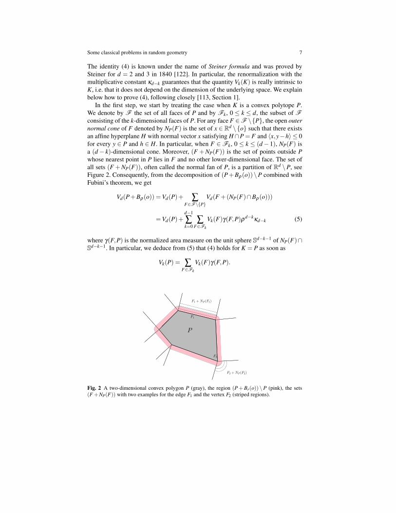
In the first step, we start by treating the case when K is a convex polytope P.We denote by F the set of all faces of P and by Fk, 0 ≤ k ≤ d, the subset of Fconsisting of the k-dimensional faces of P. For any face F ∈F \{P}, the open outernormal cone of F denoted by NP(F) is the set of x ∈ Rd \{o} such that there existsan affine hyperplane H with normal vector x satisfying H∩P = F and 〈x,y−h〉 ≤ 0for every y ∈ P and h ∈ H. In particular, when F ∈Fk, 0 ≤ k ≤ (d− 1), NP(F) isa (d− k)-dimensional cone. Moreover, (F +NP(F)) is the set of points outside Pwhose nearest point in P lies in F and no other lower-dimensional face. The set ofall sets (F +NP(F)), often called the normal fan of P, is a partition of Rd \P, seeFigure 2. Consequently, from the decomposition of (P+Bρ(o))\P combined withFubini’s theorem, we get

Vd(P+Bρ(o)) =Vd(P)+ ∑F∈F\{P}

Vd(F +(NP(F)∩Bρ(o)))

=Vd(P)+d−1

∑k=0

∑F∈Fk

Vk(F)γ(F,P)ρd−kκd−k (5)

where γ(F,P) is the normalized area measure on the unit sphere Sd−k−1 of NP(F)∩Sd−k−1. In particular, we deduce from (5) that (4) holds for K = P as soon as

Vk(P) = ∑F∈Fk

Vk(F)γ(F,P).

P

F1

F2

F2 +NP (F2)

F1 +NP (F1)

Fig. 2 A two-dimensional convex polygon P (gray), the region (P+Br(o)) \P (pink), the sets(F +NP(F)) with two examples for the edge F1 and the vertex F2 (striped regions).

8 Pierre Calka

In the second step, we derive the Steiner formula for any convex body K. In orderto define Vk(K), we use the trick to rewrite (4) for a polytope P and for several valuesof ρ , namely ρ = 1, · · · ,(d + 1). The (d + 1) equalities constitute a Vandermondesystem of (d+1) equations in (κdV0(P), · · · ,κ0Vd(P)). These equations are linearlyindependent because the Vandermonde determinant of n pairwise distinct real num-bers is different from zero. When solving the system by inverting the Vandermondematrix, we construct a sequence αk,l , 0≤ k ≤ d, 1≤ l ≤ (d +1) such that for everypolytope P and 0≤ k ≤ d,

Vk(P) =d+1

∑l=1

αk,lVd(P+Bl(o)).

It remains to check that the set of functions Vk(·) = ∑d+1l=1 αk,lVd(·+Bl(o)), 0≤ k ≤

d, defined on K d satisfies (4). This follows from the continuity of Vd , and hence ofall Vk on the space K d endowed with the Hausdorff metric and from the fact that(4) holds on the set of convex polytopes which is dense in K d .

For practical reasons, we extend the definition of intrinsic volumes to K = /0 bytaking Vk( /0) = 0 for every k ≥ 0. Of particular interest are:- the functional V0 equal to 1{K 6= /0},- the functional V1 equal to the so-called mean width up to the multiplicative constantdκd/(2κd−1),- the functional Vd−1 equal to half of the Hausdorff measure of ∂K.Furthermore, Hadwiger’s theorem, which asserts that any additive, continuous andmotion-invariant function on K d is a linear combination of the Vk’s, provides analternative way of characterizing intrinsic volumes [51].

We now go back to our initial purpose, i.e. extending the Cauchy-Crofton formulato higher dimension. We do so in two different ways:

First, when K ∈K 2, an integration over ρ in (3) shows that

L (∂K) = 2V1(K) =∫

π

0V1(K|L0,θ )dθ

where (K|L0,θ ) is the one-dimensional orthogonal projection of K onto L0,θ . WhenK ∈K d , d ≥ 2, Kubota’s formula asserts that any intrinsic volume Vk can be re-covered up to a multiplicative constant as the mean of the Lebesgue measure of theprojection of K onto a uniformly distributed random k-dimensional linear subspace.In other words, there exists an explicit positive constant c depending on d and k butnot on K such that for every K ∈K d ,

Vk(K) = c∫SOd

Vk(K|R(L))dνd(R) (6)

where L is a fixed k-dimensional linear subspace of Rd , SOd is the usual specialorthogonal group of Rd and νd is its associated normalized Haar measure.

Secondly, with a slight rewriting of (3), we get for any K ∈K 2


L (∂K) =∫∫

R×(0,π)Vo(K∩ (rotθ (L0,0)+ρ(cos(θ),sin(θ))))dρdθ ,

where rotθ is the rotation around o and of angle θ . When K ∈ K d , d ≥ 2, forany 0≤ l ≤ k≤ d and any fixed (d−k+ l)-dimensional linear subspace Ld−k+l , theCrofton formula states that the k-th intrinsic volume of K is proportional to the meanof the l-th intrinsic volume of the intersection of K with a uniformly distributedrandom (d−k+ l)-dimensional affine subspace, i.e. there exists an explicit positiveconstant c′ depending on d, k and l but not on K such that

Vk(K) = c′∫SOd

∫L⊥d−k+l

Vl(K∩ (RLd−k+l + t))dtdνd(R), (7)

where Ld−k+l is a fixed (d− k+ l)-dimensional affine subspace of Rd .For the proofs of (6) and (7) with the proper explicit constants and for a more

extensive account on integral geometry and its links to stochastic geometry, we referthe reader to the reference books [111, Chapters 13-14], [110, Chapters 4-5] and[114, Chapters 5-6]. We will show in the next section how some of the formulasfrom integral geometry are essential to derive explicit probabilities related to thePoisson hyperplane tessellation.

2 From Bertrand’s paradox to random tessellations

In this section, we recall Bertrand’s problem which leads to three different and per-fectly correct answers. This famous paradox questions the several potential modelsfor constructing random lines in the Euclidean plane. The fundamental choice ofthe translation-invariance leads us to the definition of the stationary Poisson lineprocess. After that, by extension, we survey a few basic facts on two examples ofstationary random tessellations of Rd , namely the Poisson hyperplane tessellationand the Poisson-Voronoi tessellation.

2.1 Starting from Bertrand’s paradox

In the book entitled Calcul des Probabilites and published in 1889 [12], J. Bertrandasks for the following question: a chord of the unit circle is chosen at random. Whatis the probability that it is longer than

√3, i.e. the edge of an equilateral triangle

inscribed in the circle?The paradox comes from the fact that there are several ways of choosing a chord

at random. Depending on the model that is selected, the question has several pos-sible answers. In particular, there are three correct calculations which show that therequired probability is equal to either 1/2, or 1/3 or 1/4. Still a celebrated and well-known mathematical brain-teaser, Bertrand’s problem questions the foundations of

10 Pierre Calka

the modern probability theory when the considered variables are not discrete. Wedescribe below the three different models and solutions.Solution 1: random radius. We define a random chord through the polar coordi-nates (R,Θ) of the orthogonal projection of the origin onto it. The variable Θ isassumed to be uniformly distributed on (0,2π) because of the rotation-invariance ofthe problem while R is taken independent of Θ and uniformly distributed in (0,1).The length of the associated chord is 2

√1−R2. Consequently, the required proba-

bility isp1 = P(2

√1−R2 ≥

√3) = P(R≤ 1/2) = 1/2.

Solution 2: random endpoints. We define a random chord through the position Θ ofits starting point in the anticlockwise direction and the circular length Θ ′ to its end-point. Again, Θ is uniformly distributed on (0,2π) while Θ ′ is chosen independentof Θ and also uniformly distributed in (0,2π). The length of the associated chord is2sin(Θ ′/2). Consequently, the required probability is

p2 = P(2sin(Θ ′/2)≥√

3) = P(Θ ′/2 ∈ (π/3,2π/3)) =4π

3 −2π

32π

=13.

Solution 3: random midpoint. We define a random chord through its midpoint X .The random point X is assumed to be uniformly distributed in the unit disk. Thelength of the associated chord is 2

√1−‖X‖2. Consequently, the required probabil-

ity is

p3 = P(‖X‖ ≤ 1/2) =V2(Bo(1/2))

V2(Bo(1))=

14.

Fig. 3 Simulation of Bertrand’s problem with 100 chords: (a) Solution 1 (left): 54 successful (plainline, red), 46 unsuccessful (dotted line, blue) (b) Solution 2 (middle): 30 successful (c) Solution 3(right): 21 successful.

In conclusion, as soon as the model, i.e. the meaning that is given to the wordrandom, is fixed, all three solutions look perfectly correct. J. Bertrand considers theproblem as ill-posed, that is he does not decide in favor of any of the three. Neitherdoes H. Poincare in his treatment of Bertrand’s paradox in his own Calcul des prob-


abilites in 1912 [101]. Actually, they build on it a tentative formalized probabilitytheory in a continuous space. Many years later, in his 1973 paper The well-posedproblem [68], E. T. Jaynes explains that a natural way for discriminating betweenthe three solutions consists in favoring the one which has the most invariance prop-erties with respect to transformation groups. All three are rotation invariant but onlyone is translation invariant and that is Solution 1. And in fact, in a paper from 1868[34], long before Bertrand’s book, M. W. Crofton had already proposed a way toconstruct random lines which guarantees that the mean number of lines intersectinga fixed closed convex set is proportional to the arc length of its boundary.

Identifying the set of lines Lρ,θ with R× [0,π), we observe that the previous dis-cussion means that the Lebesgue measure dρdθ on R× [0,π) plays a special rolewhen generating random lines. Actually, it is the only rotation and translation invari-ant measure up to a multiplicative constant. The construction of a natural randomset of lines in R2 will rely heavily on it.

2.2 Random sets of points, random sets of lines and extensions

Generating random geometric shapes in the plane requires to generate random setsof points and random sets of lines. Under the restriction to a fixed convex body K,the most natural way to generate random points consists in constructing a sequenceof independent points which are uniformly distributed in K. Similarly, in view ofthe conclusion on Bertrand’s paradox, random lines can be naturally taken as inde-pendent and identically distributed lines with common distribution

1µ2(K)

1{Lρ,θ∩K 6= /0}dρdθ

whereµ2(·) =

∫∫R×(0,π)

1{Lρ,θ∩· 6= /0}dρdθ .

These constructions present two drawbacks: first, they are only defined insideK and not in the whole space and secondly, they lead to undesired dependencies.Indeed, when fixing the total number of points or lines thrown in K, the joint distri-bution of the numbers of points or lines falling into several disjoint Borel subsets ofK is multinomial. Actually, there is a way of defining a more satisfying distributionon the space of locally finite sets of points (resp. lines) in the plane endowed withthe σ -algebra generated by the set of functions which to any set of points (resp.lines) associates the number of points falling into a fixed Borel set of R2 (resp. thenumber of lines intersecting a fixed Borel set of R2). Indeed, for any fixed λ > 0,there exists a random set of points (resp. lines) in the plane such that:- for every Borel set B with finite Lebesgue measure, the number of points fallinginto B (resp. the number of lines intersecting B) is Poisson distributed with meanλV2(B) (resp. λ µ2(B))

12 Pierre Calka

- for every finite collection of disjoint Borel sets B1, · · · ,Bk, k ≥ 1, the numbers ofpoints falling into Bi (resp. lines intersecting Bi) are mutually independent.

This random set is unique in distribution and both translation and rotation invari-ant. It is called a homogeneous Poisson point process (resp. isotropic and stationaryPoisson line process) of intensity λ . For a detailed construction of both processes,we refer the reader to e.g. [114, Section 3.2].

The Poisson point process can be naturally extended to Rd , d ≥ 3, by replacingV2 with Vd . Similarly, we define the isotropic and stationary Poisson hyperplaneprocess in Rd by replacing µ2 by a measure µd which is defined in the followingway. For any ρ ∈R and u ∈ Sd−1

+ , we denote by Hρ,u the hyperplane containing thepoint ρu and orthogonal to u. Let µd be the measure on Rd such that for any Borelset B of Rd ,

µd(B) =∫∫

R×Sd−1+

1{Hρ,u∩B 6= /0}dρdσd(u). (8)

Another possible extension of these models consists in replacing the Lebesguemeasure Vd (resp. the measure µd) by any locally finite measure which is not amultiple of Vd (resp. of µd). This automatically removes the translation invariancein the case of the Poisson point process while the translation invariance is preservedin the case of the Poisson hyperplane process only if the new measure is of the formdρdνd(u) where νd is a measure on Sd−1

+ . For more information on this and alsoon non-Poisson point processes, we refer the reader to the reference books [95, 36,72, 31]. In what follows, we only consider homogeneous Poisson point processesand isotropic and stationary Poisson hyperplane processes, denoted respectively byPλ and Pλ . These processes will constitute the basis for constructing stationaryrandom tessellations of the Euclidean space.

2.3 On two examples of random convex tessellations

The Poisson hyperplane process Pλ induces naturally a tessellation of Rd into con-vex polytopes called cells which are the closures of the connected components ofthe set Rd \

⋃H∈Pλ

H. This tessellation is called the (isotropic and stationary) Pois-son hyperplane tessellation of intensity λ . In dimension two, with probability one,any crossing between two lines is an X-crossing, i.e. any vertex of a cell belongsto exactly 4 different cells while in dimension d, any k-dimensional face of a cell,0≤ k≤ d, is included in the intersection of (d−k) different hyperplanes and belongsto exactly 2d−k different cells almost surely.

Similarly, the Poisson point process Pλ also generates a tessellation in the fol-lowing way: any point x of Pλ , called a nucleus, gives birth to its associated cellC(x|Pλ ) defined as the set of points of Rd which are closer to x than to any otherpoint of Pλ for the Euclidean distance, i.e.


C(x|Pλ ) = {y ∈ Rd : ‖y− x‖ ≤ ‖y− x′||∀x′ ∈Pλ}.

This tessellation is called the Voronoi tessellation generated by Pλ or the Poisson-Voronoi tessellation in short. In particular, the cell C(x|Pλ ) with nucleus x isbounded by portions of bisecting hyperplanes of segments [x,x′], x′ ∈Pλ \ {x}.The set of vertices and edges of these cells constitute a graph which is random andembedded in Rd , sometimes referred to as the Poisson-Voronoi skeleton. In dimen-sion two, with probability one, any vertex of this graph belongs to exactly threedifferent edges and three different cells while in dimension d, any k-dimensionalface of a cell, 0≤ k ≤ d, is included in the intersection of (d +1− k)(d− k)/2 dif-ferent bisecting hyperplanes and belongs to exactly (d+1−k) different cells almostsurely.

Fig. 4 Simulation of the Poisson line tessellation (left) and the Poisson-Voronoi tessellation (right)in the square.

The Poisson hyperplane tessellation has been used as a natural model for the tra-jectories of particles inside bubble chambers [46], the fibrous structure of paper [85]and the road map of a city [56]. The Voronoi construction was introduced in the firstplace by R. Descartes as a possible model for the shape of the galaxies in the Uni-verse [37]. The Poisson-Voronoi tessellation has appeared since then in numerousapplied domains, including telecommunication networks [5] and materials science[103, 76].

In both cases, stationarity of the underlying Poisson process makes it possibleto do a statistical study of the tessellation. Indeed, let f be a translation-invariant,measurable and non-negative real-valued function defined on the set Pd of convexpolytopes of Rd endowed with the topology of the Hausdorff distance. For r > 0,let Cr and Nr be respectively the set of cells included in Br(o) and its cardinality.Then, following for instance [33], we can apply Wiener’s ergodic theorem to getthat, when r→ ∞,

14 Pierre Calka

1Nr

∑C∈Cr

f (C)→ 1E(Vd(Co)−1)

E(

f (Co)

Vd(Co)

)almost surely (9)

where Co is the almost-sure unique cell containing the origin o in its interior.This implies that two different cells are of particular interest: the cell Co, often

called the zero-cell, and the cell C defined in distribution by the identity

E( f (C )) =1

E(Vd(Co)−1)E(

f (Co)

Vd(Co)

). (10)

The convergence at (9) suggests that C has the law of a cell chosen uniformly atrandom in the whole tessellation, though such a procedure would not have any clearmathematical meaning. That is why C is called the typical cell of the tessellationeven if it is not defined almost surely and it does not belong to the tessellationeither. In particular, the typical cell is not equal in distribution to the zero-cell and isactually stochastically smaller since it has a density proportional to Vd(Co)

−1 withrespect to the distribution of Co. Actually, it is possible in the case of the Poissonhyperplane tessellation to construct a realization of C which is almost surely strictlyincluded in Co [82]. This fact can be reinterpreted as a multidimensional version ofthe classical bus waiting time paradox, which says the following: if an individualarrives at time t at a bus stop, the time between the last bus he/she missed and the bushe/she will take is larger than the typical interarrival time between two consecutivebusses.

Relying on either (9) or (10) may not be easy when calculating explicit meanvalues or distributions of geometric characteristics of C . Another equivalent way ofdefining the distribution of C is provided by the use of a so-called Palm distribution,see e.g. [96], [92, Section 3.2], [114, Sections 3.3,3.4] and [75, Section 9]. For sakeof simplicity, we explain the procedure in the case of the Poisson-Voronoi tessella-tion only. Let f be a measurable and non-negative real-valued function defined onPd . Then, for any Borel set B such that 0 <Vd(B)< ∞, we get

E( f (C )) =1

λVd(B)E

(∑

x∈Pλ∩Bf (C(x|Pλ )− x)

). (11)

where C(x|Pλ )− x is the set C(x|Pλ ) translated by −x. The fact that the quantityon the right-hand side of the identity (11) does not depend on the Borel set B comesfrom the translation invariance of the Poisson point process Pλ . It is also remark-able that the right-hand side of (11) is again a mean over the cells with nucleus in Bbut contrary to (9) there is no limit involved, which means in particular that B canbe as small as one likes, provided that Vd(B)> 0.

Following for instance [92, Proposition 3.3.2], we describe below the proof of(11), i.e. that for any translation-invariant, measurable and non-negative functionf , the Palm distribution defined at (11) is the same as the limit of the means inthe law of large numbers at (9). Indeed, let us assume that C be defined in lawby the identity (11) and let us prove that (10) is satisfied, i.e. that C has a density


proportional to Vd(·)−1 with respect to Co. By classical arguments from measuretheory, (11) implies that for any non-negative measurable function F defined on theproduct space Pd×Rd ,

λ

∫E(F(C ,x))dx = E

(∑

x∈Pλ

F(C(x|Pλ )− x,x)

).

Applying this to F(C,x) = f (C)Vd(C)1{−x∈C} and using the translation invariance of f ,

we get

λE( f (C )) = E

(∑

x∈Pλ

f (C(x|Pλ ))

Vd(C(x|Pλ ))1o∈C(x|Pλ )

)= E

(f (Co)

Vd(Co)

). (12)

Applying (12) to f = 1 and f =Vd successively, we get

E(Vd(C )) =1

E(Vd(Co)−1)=

1λ. (13)

Combining (12) and (13), we obtain that the typical cell C defined at (11) satisfies(10) so it is equal in distribution to the typical cell defined earlier through the law oflarge numbers at (9).

In addition to these two characterizations of the typical cell, the Palm definition(11) of C in the case of the Poisson-Voronoi tessellation provides a very simplerealization of the typical cell C : it is equal in distribution to the cell C(o|Pλ ∪{o}),i.e. the Voronoi cell associated with the nucleus o when the origin is added to the setof nuclei of the tessellation. This result is often called Slivnyak’s theorem, see e.g.[114, Theorem 3.3.5].

The classical problems related to stationary tessellations are mainly the follow-ing:

(a)making a global study of the tessellation, for instance on the set of vertices oredges: calculation of mean global topological characteristics per unit volume,proof of limit theorems, etc;

(b)calculating mean values and whenever possible, moments and distributions ofgeometric characteristics of the zero-cell or the typical cell or a typical face;

(c)studying rare events, i.e. estimating distribution tails of the characteristics of thezero-cell or the typical cell and proving the existence of limit shapes in someasymptotic context.

Problem (a). As mentioned earlier, R. Cowan [33] showed several laws of largenumbers by ergodic methods which were followed by second-order results from theseminal work due to F. Avram and Bertsimas on central limit theorems [4] to themore recent additions [55] and [57]. Topological relationships have been recentlyestablished in [130] for a general class of stationary tessellations.

16 Pierre Calka

Problem (b). The question of determining mean values of the volume or any com-binatorial quantity of a particular cell was tackled early. The main contributionsare due notably to G. Matheron [80, Chapter 6] and R. E. Miles [87, 88] in thecase of the Poisson hyperplane tessellation and to J. Møller [90] in the case of thePoisson-Voronoi tessellation. Still, to the best of our knowledge, some mean val-ues are unknown like for instance the mean number of k-dimensional faces of thePoisson-Voronoi typical cell for 1≤ k ≤ (d−1) and d ≥ 3. Regarding explicit dis-tributions, several works are noticeable [11, 22, 23] but in the end, it seems that veryfew have been computable up to now.

Problem (c). The most significant works related to this topic have been rather re-cent: distribution tails and large-deviations type results [44, 58], extreme values [29],high dimension [59]... Nevertheless, many questions, for instance regarding preciseestimates of distribution tails, remain open to this day. One of the most celebratedquestions concerns the shape of large cells. A famous conjecture stated by D. G.Kendall in the forties asserts that large cells from a stationary and isotropic Poissonline tessellation are close to the circular shape, see e.g. the foreword to [31]. Thisremarkable feature is in fact common to the Crofton cell and the typical cell of boththe Poisson hyperplane tessellation and the Poisson-Voronoi tessellation in any di-mension. It was formalized for different meanings of large cells and proved, withan explicit probability estimate of the deviation to the limit shape, by D. Hug, M.Reitzner and R. Schneider in a series of breakthrough papers, see e.g. [63, 64, 60].

Intentionally, we have chosen to skip numerous other models of tessellations.Noteworthy among these are those generated by non-Poisson point processes [45],Johnson-Mehl tessellations [91] and especially STIT tessellations [94].

In the next subsection, we collect a few explicit first results related to Problem(b), i.e. the mean value and distribution of several geometric characteristics of eitherthe zero-cell Co or the typical cell C .

2.4 Mean values and distributional properties of the zero-cell andof the typical cell

This subsection is not designed as an exhaustive account on the many existing resultsrelated to zero and typical cells from random tessellations. Instead, we focus here onthe basic first calculations which do not require much knowledge on Poisson pointprocesses. For more information and details, we refer the reader to the referencebooks [92], [114, Section 10.4] and to the survey [23].


2.4.1 The zero-cell of a Poisson hyperplane tessellation

We start with the calculation of the probability for a certain convex body K to beincluded in Co the zero-cell or the typical cell. In the case of the planar Poissonline tessellation, let K be a convex body containing the origin - if not, K can bereplaced by the convex hull of K∪{o}. Since the number of lines from the Poissonline process intersecting K is a Poisson variable with mean λ µ2(K), we get

P(K ⊂Co) = P({Lρ,θ ∩K = /0 ∀Lρ,θ ∈Pλ )

= exp(−µ2(K))

= exp(−L (∂K)),

where the last equality comes from the Cauchy-Crofton formula (3) and is obviouslyreminiscent of Buffon’s needle problem. For d ≥ 3, we get similarly, thanks to (7)applied to k = 1 and l = 0,

P(K ⊂Co) = exp(−µd(K)) = exp(−κd−1V1(K)). (14)

The use of Crofton formula for deriving the probability P(K ⊂Co) may explain whythe zero-cell of the isotropic and stationary Poisson hyperplane tessellation is oftenreferred to as the Crofton cell.

Applying (14) to K = Br(o), r > 0, and using the equality V1(Bd) = dκdκd−1

, weobtain that the radius of the largest ball centered at o and included in Co is exponen-tially distributed with mean (dκd)

−1.

2.4.2 The typical cell of a Poisson hyperplane tessellation

Let us denote by f0(·) the number of vertices of a convex polytope. In the planarcase, some general considerations show without much calculation that E( f0(C )) isequal to 4. Indeed, we have already noted that with probability one, any vertex ofa cell belongs to exactly 4 cells and is the highest point of a unique cell. Conse-quently, there are as many cells as vertices. In particular, the mean 1

Nr∑C∈Cr f0(C)

is equal, up to boundary effects going to zero when r→∞, to 4 times the ratio of thetotal number of vertices in Br(o) over the total number of cells included in Br(o),i.e. converges to 4. Other calculations of means and further moments of geometriccharacteristics can be found notably in [80, Chapter 6] and in [85, 86, 87].

One of the very few explicit distributions is the law of the inradius of C , i.e.the radius of the largest ball included in C . Remarkably, this radius is equal indistribution to the radius of the largest ball centered at o and included in Co, i.e. isexponentially distributed with mean (dκd)

−1. This result is due to R. E. Miles indimension two and is part of an explicit construction of the typical cell C basedon its inball [88], which has been extended to higher dimension since then, see e.g.[24].

18 Pierre Calka

2.4.3 The typical cell of a Poisson-Voronoi tessellation

In this subsection, we use the realization of the typical cell C of a Poisson-Voronoitessellation as the cell C(o|Pλ ∪{o}), as explained at the end of Subsection 2.3. Wefollow the same strategy as for the zero-cell of a Poisson hyperplane tessellation, i.e.calculating the probability for a convex body K to be contained in C and deducingfrom it the distribution of the inradius of C .

Let K be a convex body containing the origin. The set K is contained in C(o|Pλ ∪{o}) if and only if o is the nearest nucleus to any point in K, which means that forevery x ∈ K, the ball B‖x‖(x) does not intersect Pλ . Let us consider the set

Fo(K) =⋃x∈K

B‖x‖(x)

that we call the Voronoi flower of K with respect to o, see Figure 5.

o

K

Fo(K)

Fig. 5 Voronoi Flower (red) of the convex body K (black) with respect to o.

Using the fact that the number of points of Pλ in Fo(K) is Poisson distributedwith mean λVd(Fo(K)), we get

P(K ⊂C(o|Pλ ∪{o})) = exp(−λVd(Fo(K))).

Applying this to K = Bo(r), r > 0, we deduce that the radius of the largest ball cen-tered at o and included in C(o|Pλ ∪{o}) is Weibull distributed with tail probabilityequal to exp(−λ2dκdrd), r > 0.

Similarly to the case of the typical cell of a Poisson line tessellation, some directarguments lead us to the calculation of E( f0(C )) in dimension two: any vertex ofa cell belongs to exactly 3 cells and with probability one, is the either highest orlowest point of a unique cell. Consequently, there are as twice as many vertices ascells. In particular, the mean 1

Nr∑C∈Cr f0(C) is equal, up to boundary effects going

to zero when r→ ∞, to 3 times the ratio of the total number of vertices in Br(o)over the total number of cells included in Br(o), i.e. equal to 6. This means thatE( f0(C )) = 6.

In the next section, we describe a different way of generating random polytopes:they are indeed constructed as convex hulls of random sets of points.


3 From Sylvester’s four-point problem to random polytopes

This section is centered around Sylvester’s four-point problem, another historicalproblem of geometric probability which seemingly falls under the denomination ofrecreational mathematics but in fact lays the foundations of an active domain oftoday’s stochastic geometry, namely the theory of random polytopes. We aim atdescribing first Sylvester’s original question and some partial answers to it. We thensurvey the topic of random polytopes which has been largely investigated since thesixties, partly due to the simultaneous development of computational geometry.

3.1 Starting from Sylvester’s four-point problem

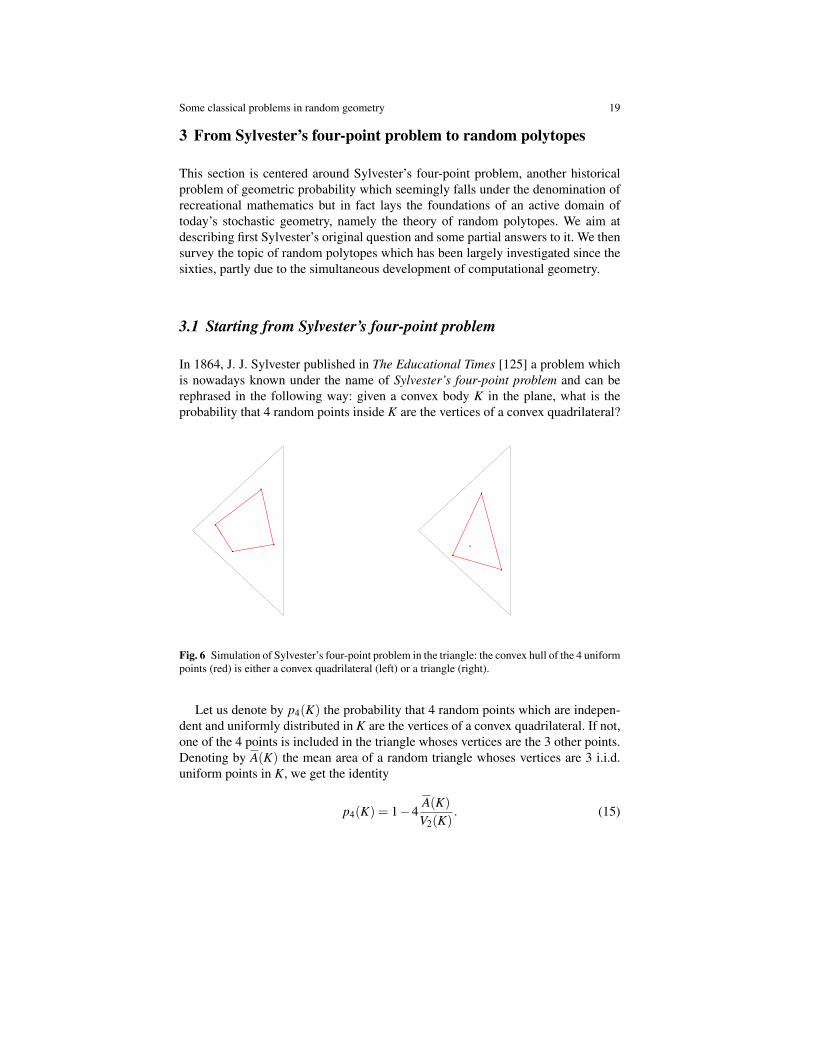
In 1864, J. J. Sylvester published in The Educational Times [125] a problem whichis nowadays known under the name of Sylvester’s four-point problem and can berephrased in the following way: given a convex body K in the plane, what is theprobability that 4 random points inside K are the vertices of a convex quadrilateral?

Fig. 6 Simulation of Sylvester’s four-point problem in the triangle: the convex hull of the 4 uniformpoints (red) is either a convex quadrilateral (left) or a triangle (right).

Let us denote by p4(K) the probability that 4 random points which are indepen-dent and uniformly distributed in K are the vertices of a convex quadrilateral. If not,one of the 4 points is included in the triangle whoses vertices are the 3 other points.Denoting by A(K) the mean area of a random triangle whoses vertices are 3 i.i.d.uniform points in K, we get the identity

p4(K) = 1−4A(K)

V2(K). (15)

20 Pierre Calka

Solving Sylvester’s problem is then equivalent to calculating the mean value A(K).In particular, the quantity A(K)

V2(K) is scaling invariant and also invariant under anyarea-preserving affine transformation.

3.1.1 Calculation of Sylvester’s probability in the case of the disk

In this subsection, we provide an explicit calculation of p4(D) where D is the unitdisk. As in the next subsection, we follow closely the method contained in [70, pages42-46].

Step 1. We can assume that one of the points is on the boundary of the disk. In-deed, isolating the farthest point from the origin, we get

V2(D)3A(D) = 3∫D

[∫∫D2

1{‖x1‖,‖x2‖∈(0,‖x3‖)}V2(Conv({x1,x2,x3})))dz1dz2

]dz3.

Now for a fixed z3 ∈D\{o}, we apply the change of variables z′i =zi‖z3‖

, i = 1,2, inthe double integral and we deduce that

A(D) =3

π3

∫D‖z3‖6

[∫∫D2

V2(Conv({z′1,z′2,z3

‖z3‖})))dz′1dz′2

]dz3.

(16)

Since the double integral above does not depend on z3, we get

A(D) =3

4π2 I (17)

whereI =

∫∫D2

V2(Conv({z0,z1,z2}))dz1dz2,

z0 being a fixed point on the boundary of D.

Step 2. Let us now calculate I, i.e. π2 times the mean area of a random trianglewith one deterministic vertex on the unit circle and two random vertices indepen-dent and uniformly distributed in D.

For sake of simplicity, we replace the unit disk D by its translate D+(0,1) andthe fixed point on the boundary of D+(0,1) is chosen to be equal to o. This doesnot modify the integral I. The polar coordinates (ρi,θi) of zi, i = 1,2, satisfy ρi ∈(0,2sin(θi)) and

V2(Conv({o,z1,z2})) =12

ρ1ρ2|sin(θ2−θ1)|. (18)

Consequently, we obtain


I =∫∫

0<θ1<θ2<π

[∫ 2sin(θ1))

0ρ

21 dρ1

∫ 2sin(θ2)

0ρ

22 dρ2

]sin(θ2−θ1)dθ1dθ2

=649

∫∫0<θ1<θ2<π

sin3(θ1)sin3(θ2)sin(θ2−θ1)dθ1dθ2

=35π

36.

Conclusion. Combining this result with (17) and (15), we get

p4(D) = 1− 3512π2 ≈ 0.70448...

3.1.2 Calculation of Sylvester’s probability in the case of the triangle

In this subsection, we calculate the probability p4(T) where the triangle T is theconvex hull of the three points o, (1,1) and (1,−1). We recall that the calculationof p4(K) is invariant under any area-preserving affine transformation.

Step 1. We can assume that one of the points is on the edge facing o. Indeed, denot-ing by (xi,yi) the Cartesian coordinates of zi, i = 1,2,3, we get

V2(T)3A(T) = 3∫T

[∫∫T2

1{x1,x2∈(0,x3)}V2(Conv({z1,z2,z3}))dz1dz2

]dz3.

Now for a fixed z3 ∈ T \ {o}, we apply the change of variables z′i =zix3

, i = 1,2, inthe double integral. We get

A(T) = 3∫ 1

x3=0

∫ x3

y3=−x3

[∫∫T2

x63V2(Conv({z′1,z′2,

z3

x3}))dz′1dz′2

]dz3

= 6∫ 1

x3=0

∫ x3

y3=0x6

3

[∫∫T2

V2(Conv({z′1,z′2,x3

x3}))dz′1dz′2

]dz3.

Finally, for fixed x3, we apply the change of variables h = y3x3

. Since the doubleintegral in square brackets above does not depend on x3, we get

A(T) = 6∫ 1

0x7

3dx3

∫ 1

h=0

[∫∫T2

V2(Conv({z1,z2,(1,h)}))dz1dz2

]dh

=34

∫ 1

h=0I′(h)dh (19)

where I′(h) =∫∫

T2 V2(Conv({z1,z2,(1,h)}))dz1dz2.

Step 2. Let us now calculate I′(h), 0 < h < 1, i.e. the mean area of a random trianglewith one deterministic vertex at (1,h) on the vertical edge and two random verticesindependent and uniformly distributed in T. The point (1,h) divides T into two sub-

22 Pierre Calka

triangles, the upper triangle T+(h) = Conv({o,(1,h),(1,1)}) and the lower triangleT−(h) = Conv({o,(1,h),(1,−1)}). Let us rewrite I′(h) as

I′(h) = 2I′+,−(h)+V2(T+(h))2A(T+(h))+V2(T−(h))2A(T−(h)) (20)

where

I′+,−(h) =∫

z1∈T+(h),z2∈T−(h)V2(Conv({z1,z2,(1,h)})))dz1dz2 (21)

and A(T ), for a triangle T , is the mean area of a random triangle which shares acommon vertex with T and has two independent vertices uniformly distributed in T .

We start by making explicit the quantity A(T ) for any triangle T . It is invariantunder any area-preserving affine transformation and is multiplied by λ 2 when T isrescaled by λ−1. Consequently, it is proportional to V2(T ), i.e.

A(T ) = A(T)V2(T ). (22)

We now calculate

A(T) =∫T2

V2(Conv({o,z1,z2}))dz1dz2.

The polar coordinates (ρi,θi) of xi, i = 1,2, satisfy ρi ∈ (0,cos−1(θi)) and equality(18). Consequently, we obtain

A(T) =∫ π

4

− π4

∫ π4

− π4

[∫ cos−1(θ1)

0ρ

21 dρ1

∫ cos−1(θ2)

0ρ

22 dρ2

]sin(θ2−θ1)dθ1dθ2

=19

∫∫− π

4 <θ1<θ2<π4

sin(θ2−θ1)

cos3(θ1)cos3(θ2)dθ1dθ2

=4

27. (23)

Combining (22) and (23), we obtain in particular that

A(T+(h)) =2(1−h)

27, and A(T−(h)) =

2(1+h)27

. (24)

We turn now our attention to the quantity I′+,−(h) defined at (21). Using the rewritingof the area of a triangle as half of the non-negative determinant of two vectors andintroducing g+(h) (resp. g−(h)) as the center of mass of T+(h) (resp. T−(h)), weobtain


I′+,−(h) =12

∫z1∈T+(h),z2∈T−(h)

det(z1− (1,h),z2− (1,h))dz1dz2

=12

∫z1∈T+(h)

det((z1− (1,h)),

∫z2∈T−(h)

(z2− (1,h)))

dz1

=V2(T−(h))

2det(∫

z1∈T+(h)(z1− (1,h))dz1,(g−(h)− (1,h))

)=V2(T−(h))V2(T+(h))V2(Conv({g+(h),g−(h),(1,h)}))

=(1−h)(1+h)

4V2(T)

9=

1−h2

36. (25)

Inserting (24) and (25) into (20), we get

I′(h) =1−h2

18+

(1−h)3

54+

(1+h)3

54=

5+3h2

54. (26)

Conclusion. Combining (26) with (19) and (15), we get A(T) = 112 and

p4(T ) =23= 0.66666...

3.1.3 Extremes of p4(K)

In 1917, W. Blaschke proved a monotonicity result for Sylvester’s four-point prob-lem, namely that the probability p4(K) is maximal when K is a disk and minimalwhen K is a triangle, see [15] and [16, §24, §25]. Because of (15), this amountsto saying that the mean area of a random triangle in a unit area convex body K isminimal when K is a disk and maximal when K is a triangle.

This assertion is due to the use of symmetrization techniques which have be-come classical since then in convex and integral geometry. We describe below themain arguments developed by W. Blaschke and also rephrased in a nice way in thehistorical note [100].

Let K be a unit area convex body of R2 and let us denote by xmin and xmax theminimal and maximal projection on the x-axis of a point of K. The boundary of Kis parametrized by two functions f+, f− : [xmin,xmax] −→ R such that f+ ≥ f− withequality at xmin and xmax. We use the term Steiner symmetrization of K with respect tothe x-axis for the transformation

S :

{K −→ R2

(x,y) 7−→(

x,y− f+(x)+ f−(x)2

)In other words, S sends any segment which is the intersection of K with a verticalline to its unique vertical translate which is symmetric with respect to the x-axis; seeFigure 7. In particular, S is area-preserving and the image of K is a convex bodywhich is symmetric with respect to the x-axis, see e.g. [110, Section 10.3]. Let us

24 Pierre Calka

show thatA(K)≥ A(S (K)) (27)

Let zi = (xi,yi), i = 1,2,3, be three points of K. In particular, we start by noticingthat the area of the parallelogram spanned by the two vectors (z2− z1) and (z3− z1)is twice the area of the triangle Conv({z1,z2,z3}). Consequently, we get

V2(Conv({z1,z2,z3}) =12|∣∣∣∣ x2− x1 x3− x1y2− y1 y3− y1

∣∣∣∣ |= 12|

∣∣∣∣∣∣1 1 1x1 x2 x3y1 y2 y3

∣∣∣∣∣∣ |. (28)

We will also use the points z∗i = S (zi) = (xi,y∗i ), zi∗ = (xi,−y∗i ) and wi = (xi,yi−2y∗i ), i = 1,2,3. In particular, the identity S (wi) = zi∗ is satisfied and the two trian-gles Conv({z1,z2,z3}) and Conv({w1,w2,w3}) have same area. Consequently,

V2(Conv({z1,z2,z3})+V2(Conv({w1,w2,w3})

≥ 12|

∣∣∣∣∣∣1 1 1x1 x2 x3y1 y2 y3

∣∣∣∣∣∣−∣∣∣∣∣∣

1 1 1x1 x2 x3

y1−2y∗1 y2−2y∗2 y3−2y∗3

∣∣∣∣∣∣ |≥ 1

2|

∣∣∣∣∣∣1 1 1x1 x2 x32y∗1 2y∗2 2y∗3

∣∣∣∣∣∣ |= 2V2(Conv({z∗1,z∗2,z∗3})). (29)

Integrating (29) with respect to z1,z2,z3 ∈K and using the fact that both the transfor-mation S and the reflection with respect to the x-axis preserve the Lebesgue mea-sure, we obtain (27). It remains to use the fact that the equality in (27) is satisfiedonly when K is an ellipse. In fact, for any convex body K, there exists a sequence oflines such that the image of K under consecutive applications of Steiner symmetriza-tions with respect to the lines of that sequence converges to a disk [26]. The functionA(·) being continuous on the set of convex bodies, we obtain A(K) ≥ A( 1√

πD) and

therefore p4(K)≤ p4(D).We turn now our attention to the proof of p4(K) ≤ p4(T). The method relies

on a transformation T in the same spirit as the Steiner symmetrization, calledSchuttelung or shaking and defined as follows:

T ::{

K −→ R2

(x,y) 7−→ (x,y− f−(x))

In other words, T sends any segment which is the intersection of K with a verticalline to its unique vertical translate with a lower-end on the x-axis, see Figure 7. Inparticular, T is area-preserving and preserves the convexity.

Using both (28) and the fact that K is a unit-area convex body which satisfies theequality

K = {(x,y) : x ∈ [xmin,xmax], f−(x)≤ y≤ f+(x)},


Fig. 7 Two symmetrizations (red) of a convex body delimited by translates of the curves f+(x) =√x and f−(x) = x(x− 2+

√2

2 ) on the interval [0,2] (black) and the image of a triangle by sym-metrization (blue): the Steiner symmetrization (left) and the shaking (right).

we get that

A(K) =∫∫∫

[xmin,xmax]I(x1,x2,x3)dx1dx2dx3 (30)

where

I(x1,x2,x3)

=∫ f+(x1)

f−(x1)

∫ f+(x2)

f−(x2)

∫ f+(x3)

f−(x3)

12|

∣∣∣∣∣∣1 1 1x1 x2 x3y1 y2 y3

∣∣∣∣∣∣ |dy3dy2dy1

=∫ f+(x1)

f−(x1)

∫ f+(x2)

f−(x2)

∫ f+(x3)

f−(x3)

12|a1y1 +a2y2 +a3y3|dy3dy2dy1.

and with a1 = a1(x1,x2,x3) = (x3− x2), a2 = a2(x1,x2,x3) = (x1− x3) and a3 =a3(x1,x2,x3) = (x2− x1). For sake of simplicity, the dependency of the coefficientsai on the coordinates xi is omitted. When x1,x2,x3 are fixed, the function I calculatesthe 4-dimensional volume of the parallelepiped region delimited by the rectangularbasis [ f−(x1), f+(x1)]× [ f−(x2), f+(x2)]× [ f−(x3), f+(x3)]×{0} and the surface ofequation y4 =

12 |a1y1 + a2y2 + a3y3| . In particular, if we allow the rectangular ba-

sis to be translated, the integral I only depends on the distance D in R3 from themidpoint ( f−(x1)+ f+(x1)

2 , f−(x2)+ f+(x2)2 , f−(x3)+ f+(x3)

2 ) of the rectangular basis to theset {(y1,y2,y3) : a1y1 + a2y2 + a3y3 = 0} and is even an increasing function of D .We notice that D satisfies

26 Pierre Calka

D =|a1( f−(x1)+ f+(x1))+a2( f−(x2)+ f+(x2))+a3( f−(x3)+ f+(x3))|

2√

a21 +a2

2 +a23

=1

2√

a21 +a2

2 +a23

|

∣∣∣∣∣∣1 1 1x1 x2 x3

f−(x1) f−(x2) f−(x3)

∣∣∣∣∣∣+∣∣∣∣∣∣

1 1 1x1 x2 x3

f+(x1) f+(x2) f+(x3)

∣∣∣∣∣∣ |.Now, the two determinants in the last equality above are two times the algebraicareas of two triangles whose vertices are on ∂K and have respective x-coordinatesx1, x2 and x3. Because of the convexity of K, they must have opposite signs. Conse-quently, we get from the triangular inequality ||a|− |b|| ≤ |a−b| that

D ≤ 1

2√

a21 +a2

2 +a23

|

∣∣∣∣∣∣1 1 1x1 x2 x3

f+(x1)− f−(x1) f+(x2)− f−(x2) f+(x3)− f−(x3)

∣∣∣∣∣∣ |.In particular, after application of the transformation T , the distance is equal to theright-hand side of the inequality above. The integral I(x1,x2,x3) being an increasingfunction of D , it is greater, which implies thanks to (30) that

A(K)≤ A(T (K)).

It remains to use the fact that there exists a sequence of lines such that the image ofK under consecutive applications of the Schuttelung operations with respect to theselines converges to a triangle [13]. Therefore, we get the inequality A(K)≤ A(T) andthanks to (15), the required inequality p4(K)≥ p4(T).

3.2 Random polytopes

There are several ways of extending Sylvester’s initial question:

(a)increasing the number of random points inside K and ask for the probability thatn i.i.d. points uniformly distributed in a two-dimensional convex body K are inconvex position, i.e. are extreme points of their convex hull;

(b)increasing the dimension and ask for the probability that (d + 2) or more i.i.d.points uniformly distributed in a d-dimensional convex body K are the verticesof a convex polytope;

(c) increasing the number of random points in any dimension and ask more generalquestions, such as the distribution and mean value of the number of extremepoints and of other characteristics of the convex hull;

(d)replacing the uniform distribution in K by another probability distribution in Rd .

The topic of random polytopes has become more popular in the last 50 years andthis is undoubtedly due in part to the birth of computational geometry and the needto get quantitative information on the efficiency of algorithms in discrete geometry,


in particular algorithms designed for the construction of the convex hull of multi-variate data. We describe below the state of the art on each of the problems above.

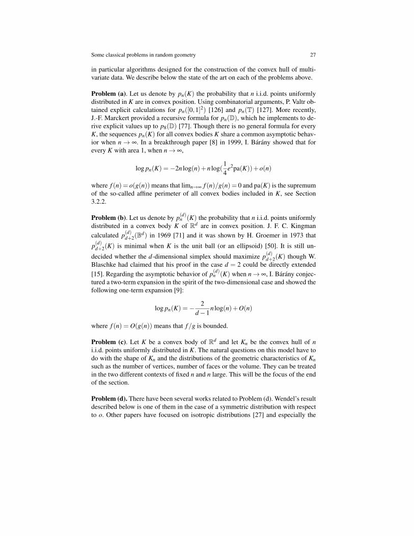
Problem (a). Let us denote by pn(K) the probability that n i.i.d. points uniformlydistributed in K are in convex position. Using combinatorial arguments, P. Valtr ob-tained explicit calculations for pn([0,1]2) [126] and pn(T) [127]. More recently,J.-F. Marckert provided a recursive formula for pn(D), which he implements to de-rive explicit values up to p8(D) [77]. Though there is no general formula for everyK, the sequences pn(K) for all convex bodies K share a common asymptotic behav-ior when n→ ∞. In a breakthrough paper [8] in 1999, I. Barany showed that forevery K with area 1, when n→ ∞,

log pn(K) =−2n log(n)+n log(14

e2pa(K))+o(n)

where f (n) = o(g(n)) means that limn→∞ f (n)/g(n) = 0 and pa(K) is the supremumof the so-called affine perimeter of all convex bodies included in K, see Section3.2.2.

Problem (b). Let us denote by p(d)n (K) the probability that n i.i.d. points uniformlydistributed in a convex body K of Rd are in convex position. J. F. C. Kingmancalculated p(d)d+2(B

d) in 1969 [71] and it was shown by H. Groemer in 1973 that

p(d)d+2(K) is minimal when K is the unit ball (or an ellipsoid) [50]. It is still un-

decided whether the d-dimensional simplex should maximize p(d)d+2(K) though W.Blaschke had claimed that his proof in the case d = 2 could be directly extended[15]. Regarding the asymptotic behavior of p(d)n (K) when n→ ∞, I. Barany conjec-tured a two-term expansion in the spirit of the two-dimensional case and showed thefollowing one-term expansion [9]:

log pn(K) =− 2d−1

n log(n)+O(n)

where f (n) = O(g(n)) means that f/g is bounded.

Problem (c). Let K be a convex body of Rd and let Kn be the convex hull of ni.i.d. points uniformly distributed in K. The natural questions on this model have todo with the shape of Kn and the distributions of the geometric characteristics of Knsuch as the number of vertices, number of faces or the volume. They can be treatedin the two different contexts of fixed n and n large. This will be the focus of the endof the section.

Problem (d). There have been several works related to Problem (d). Wendel’s resultdescribed below is one of them in the case of a symmetric distribution with respectto o. Other papers have focused on isotropic distributions [27] and especially the

28 Pierre Calka

Gaussian distribution, see e.g. [108, 10].

For a more detailed account on the topic of random polytopes, we refer the readerto [114, Chapter 8], the lecture [60] and the very exhaustive survey [107]. In the restof the section, we will present a few results related to Problem (c) in both the non-asymptotic and asymptotic regimes.

3.2.1 Non-asymptotic results

In this subsection, we describe two of the non-asymptotic results on the convexhull Kn of n i.i.d. points uniformly distributed in a convex body K of Rd : the Efronidentity relating first moments of functionals of Kn and Wendel’s calculation of theprobability that the origin o belongs to Kn. In the sequel, fk(·) is the number of k-dimensional faces of a convex polytope. In particular, f0(·) denotes the number ofvertices.

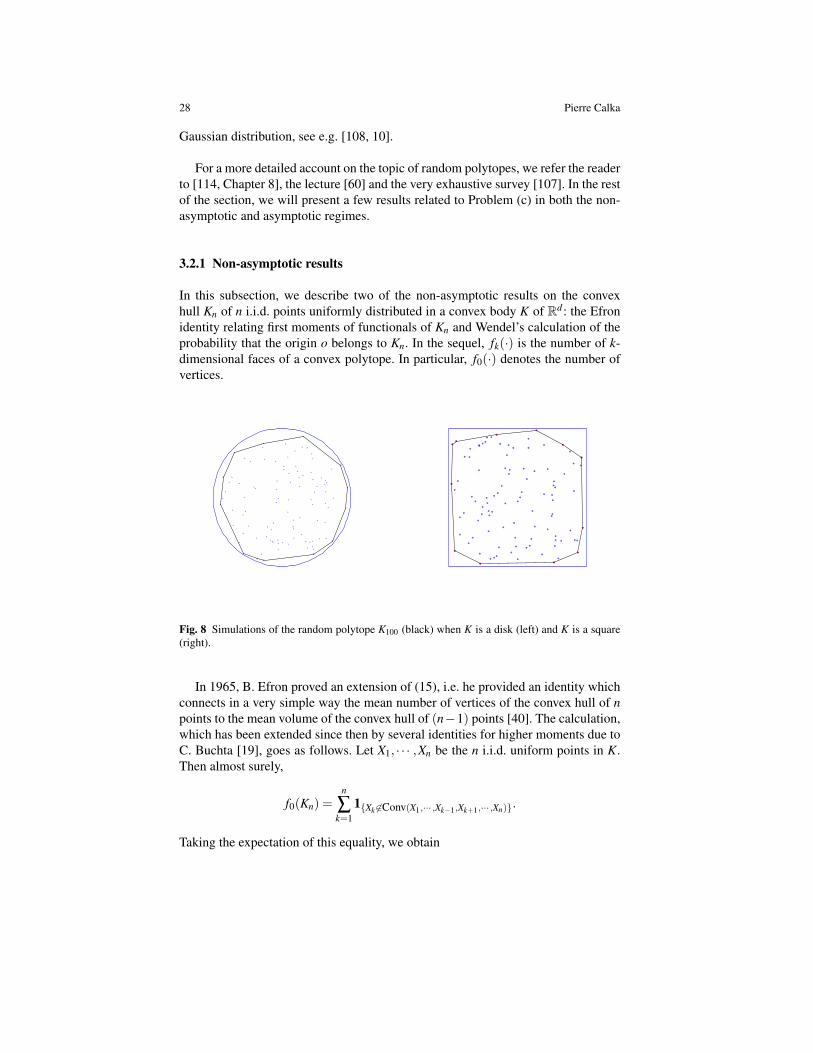
Fig. 8 Simulations of the random polytope K100 (black) when K is a disk (left) and K is a square(right).

In 1965, B. Efron proved an extension of (15), i.e. he provided an identity whichconnects in a very simple way the mean number of vertices of the convex hull of npoints to the mean volume of the convex hull of (n−1) points [40]. The calculation,which has been extended since then by several identities for higher moments due toC. Buchta [19], goes as follows. Let X1, · · · ,Xn be the n i.i.d. uniform points in K.Then almost surely,

f0(Kn) =n

∑k=1

1{Xk 6∈Conv(X1,··· ,Xk−1,Xk+1,··· ,Xn)}.

Taking the expectation of this equality, we obtain


E( f0(Kn)) = nP(Xn 6∈ Conv(X1, · · · ,Xn−1))

= nE(E(1{Xn 6∈Conv(X1,··· ,Xn−1)}|X1, · · · ,Xn−1)

= n(

1− E(Vd(Kn−1))

Vd(K)

).

In 1962, J. G. Wendel showed an explicit formula for the probability that the origin olies inside the convex hull of n i.i.d. points with a symmetric distribution with respectto o [131]. Let X1, · · · ,Xn, n≥ 1, be the random points and we assume additionallythat their common distribution is such that with probability one, all subsets of sized are linearly independent. We first notice that o is not in the convex hull if and onlyif there exists a half-space containing all the points, i.e. there exists y ∈ Rd suchthat 〈y,Xk〉 > 0 for every 1 ≤ k ≤ n. This implies in particular that the probabilityP(o 6∈ Conv({X1, · · · ,Xn})) equals 1 as soon as n≤ d and 2−(n−1) when d = 1. Nowthe calculation for n≥ (d +1)≥ 3 is done by purely combinatorial arguments.

Indeed, each Xk defines a set of authorized y which is a half-space bounded by thelinear hyperplane Hk with normal vector Xk. Consequently, each connected compo-nent of the complement of

⋃nk=1 Hk can be coded by a sequence in {−1,1}n where

+1 at the k-th position means that the connected component lies in the authorizedhalf-space bounded by Hk. There are 2n possible codes and we denote by Nd,n thetotal number of connected components. The variable Nd,n is almost surely constant,as we shall see later on. Recalling from the earlier discussion that a necessary andsufficient condition to have the origin outside of the convex hull is that the intersec-tion of all authorized half-spaces bounded by the hyperplanes Hk is not empty, weobtain the following equivalence: o is not in the convex hull of {X1, · · · ,Xn} if andonly if one of the connected components is coded by (1, · · · ,1). This happens withprobability

P(o 6∈ Conv({X1, · · · ,Xn}) =Nd,n

2n . (31)

As announced earlier, the variable Nd,n is constant on the event of probability onethat any subset of size d of the n points is linearly independent. We calculate Nd,non this event by proving a recurrence relation. For fixed n ≥ 2, the n-th hyperplaneHn separates into two subparts each connected component of Rd \

⋃n−1k=1 Hk that it

meets and leaves unchanged the remaining connected components of Rd \⋃n−1

k=1 Hk.The number of connected components of Rd \

⋃n−1k=1 Hk that Hn meets is equal to the

number of connected components of Hn \⋃n−1

k=1 Hk, i.e. Nd−1,n−1 while the numberof untouched connected components of Rd \

⋃n−1k=1 Hk is Nd,n−1−Nd−1,n−1. Conse-

quently, we get the relation

Nd,n = Nd−1,n−1 +Nd,n−1.

Using that Nd,1 = 2 for every d ≥ 1, we deduce that Nd,n = 2∑d−1k=0

(n−1k

)thanks to

Pascal’s triangle. This last equality combined with (31) leads to

30 Pierre Calka

P(o 6∈ Conv({X1, · · · ,Xn}) = 2−(n−1)d−1

∑k=0

(n−1

k

).

In particular, when n→ ∞, this probability goes to zero exponentially fast. In thenext section, we investigate the general asymptotic behavior of Kn.

3.2.2 Asymptotic results

When n→ ∞, Kn converges to K itself and studying the asymptotic behavior of Knmeans being able to quantify the quality of the approximation of K by Kn. The firstbreakthrough is due to A. Renyi and R. Sulanke in 1963 and 1964 [108, 109]. Theyshowed in particular that in the planar case, the mean number of vertices of Kn has abehavior which is highly dependent on the regularity of the boundary of K. Indeed,when ∂K is of class C 2,

E( f0(Kn)) ∼n→∞

213 3−

13 Γ

(53

)Vd(K)−

13

∫∂K

r− 1

3s dsn

13 . (32)

where rs is the radius of curvature of ∂K at s and f (n) ∼n→∞

g(n) means that f/g has

limit 1. The quantity∫

∂K r− 1

3s ds is called the affine perimeter of K.

When K is a convex polygon itself, the number of vertices of Kn is expected tobe smaller in mean as, roughly speaking, it does not require many edges to approx-imate the flat parts of the boundary of K. While the extreme points of Kn are moreor less homogeneously spread along the curve ∂K when it is smooth, they are con-centrated in the corners, i.e. around the vertices of K when K is a convex polygon.Consequently, the growth rate of E( f0(Kn)) becomes logarithmic, as opposed tothe polynomial rate from (32). Denoting by r the number of vertices of the convexpolygon K, we get

E( f0(Kn)) ∼n→∞

2r3

logn. (33)

The two estimates (32) and (33) have been extended in many directions: asymp-totic means of fk(Kn), 1≤ k ≤ d and of Vd(Kn) in any dimension and convergences[7, 106], same for the intrinsic volumes in the smooth case [116, 104], concentra-tion estimates [128], second-order results [105, 25] and so on. Many basic questionsremain unanswered, like for instance the asymptotic behavior of the mean intrinsicvolumes of Kn when K is a polytope.

In the next section, we generate for the first time non-convex random sets asunions of translates of a so-called grain.


4 From the bicycle wheel problem to random coverings andcontinuum percolation

In this section, we start with a practical problem which can be reinterpreted as arandom covering problem on the circle by random arcs with fixed length. We solveit and discuss possible extensions. This leads us to a classical model of random cov-ering of the Euclidean space called the Boolean model and we present briefly someof the questions related to it: covering of a particular set, continuum percolation andshapes of the connected components of the two phases.

4.1 Starting from the bicycle wheel problem and random coveringof the circle

In 1989, C. Domb tells how his work during the second World War in radar researchfor the Admiralty led him to ask H. Jeffreys in 1946 about a covering problem [38].H. Jeffreys related his question to his own bicycle wheel problem which he hadformulated several years before in the following way: a man is cycling along a roadand passes through a region threwn with tacks. He wishes to know whether one hasentered his tire. Because of the traffic, he can only snatch glances at random times.At each glance he has covered a fraction x of the wheel. What is the probability thatafter n glances, he has covered the whole wheel?. It turns out that the problem hadbeen solved by W. L. Stevens in 1939 [123], see also [121, Chapter 4]. Surprisingly,his method that we describe below relies exclusively on combinatorial arguments.

We start by rephrasing the problem in mathematical terms in the following way:a set of n intervals of length x are placed randomly on a circle of length one and weaim at calculating the probability qn(x) that the circle is fully covered. The endpoints

Fig. 9 Simulations of the bicycle wheel problem for x = 0.01: the random intervals in the casesn = 20 (left), n = 50 (middle) and n = 100 (right).

in the anticlockwise direction of the n random intervals of length x are denoted by

32 Pierre Calka

U1, · · · ,Un and are assumed to be n i.i.d. random variables uniformly distributed in(0,1). For every 1≤ i≤ n, we consider the event denoted by Ai that the endpoint ofthe i-th arc is not covered by the other (n−1) random intervals. The key idea consistsin noticing that the circle is fully covered by the n random intervals if and only ifall endpoints are covered. Consequently, using the inclusion-exclusion principle, weobtain that the probability pcov(n,x) satisfies

1− pcov(n,x) = P(∪ni=1Ai)

=n

∑k=1

(−1)k+1∑

1≤i1<i2<···<ik≤nP(Ai1 ∩Ai2 ∩·· ·∩Aik

)=

n

∑k=1

(−1)k+1(

nk

)P(A1∩A2∩·· ·Ak), (34)

where the last equality comes from the fact that the variables U1, · · · ,Un are ex-changeable. It remains to calculate P(A1∩A2∩·· ·Ak), 1≤ k≤ n, i.e. the probabilitythat the endpoint of each of the first k random intervals is not covered, not only bythe (k− 1) other intervals from the first bunch but also by the (n− k) remainingintervals. This means that the event A1∩A2∩·· ·Ak can be rewritten as

A1∩A2∩·· ·Ak = Bk⋂( n⋂

i=k+1

Ci,k

)(35)

where Bk is the event that the endpoint of each of the first k random intervals is notcovered by the (k−1) other intervals from the first bunch and Ci,k, k+1≤ i≤ n, isthe event that the i-th random arc does not cover any of the endpoints from the firstk random intervals.

On the event Bk, the k endpoints are at distance at least x from each other. Con-sequently, P(Bk) is the probability that a random division of the circle into k partsproduces parts of lengths larger than x. This is in particular the exact problem 666that W. A. Whitworth solves in his book Choice and Chance published in 1870[132]. By a direct integral calculation, we get

P(Bk) = (1− kx)k−1+ . (36)

Conditional on the positions of the first k random intervals which satisfy the condi-tion of the event Bk, the events Ci,k are independent. The set of allowed positions onthe circle for the endpoint of the i-th random arc is then the complement of a unionof k disjoint intervals of length x. Consequently,

P( n⋂

i=k+1

Ci,k∣∣Bk)= (1− kx)n−k

+ . (37)

Combining (36), (37) with (35) and (34) shows that


pcov(n,x)(x) =n

∑k=0

(−1)k(

nk

)(1− kx)n−1

+ .

In 1982, the formula was extended by A. F. Siegel and L. Holst to the explicit calcu-lation of pcov(n,µ), i.e. the probabiity to cover the circle with i.i.d. intervals whichhave random lengths such that these lengths are i.i.d. µ-distributed variables whichare independent of the positions of the intervals on the circle [120]. They even pro-vided the distribution of the number of uncovered gaps on the circle in this context.Following their work, T. Huillet obtained the joint distribution of the lengths of theconnected components [65]. In [119], A. F. Siegel conjectured that pcov(n,µ) sat-isfies a monotonicity result which is proved in [22] and is the following: if twoprobability distributions µ,ν on (0,1) are such that µ ≤ ν for the convex order,see e.g. [93, Chapter 1], then pcov(n,µ)≤ pcov(n,µ). In particular, thanks to Jensen’sinequality, this implies that pcov(n,x)≤ pcov(n,µ) where x is the mean of µ .

To the best of our knowledge, the most recent contribution in higher dimensionis due to P. Burgisser, F. Cucker and M. Lotz [21] and contains on one hand an exactformula for the probability to cover the sphere with n spherical caps of fixed angularradius when this radius is larger than π/2 and on the other hand an upper bound forthis probability when the angular radius is less than π/2.

Finally, a related question introduced by A. Dvoretzky in 1956 concerns the cov-ering of the circle by an infinite number of intervals (In)n with deterministic lengths(`n)n such that the sequence (`n)n is non-increasing [39]. In 1972, L. A. Sheppshowed that the circle is covered infinitely often with probability 1 if and only if theseries ∑

∞n=1 n−2 exp(`1 + · · ·+ `n) is divergent [118].

4.2 A few basics on the Boolean model

A natural extension of the bicycle wheel problem consists in considering randomcoverings of the Euclidean space by so-called grains with random positions andpossibly random shapes or sizes. Considering the discussion on the translation in-variance in Section 2, we construct directly such a model in Rd . Let Pλ be a homo-geneous Poisson point process of intensity λ and let K be a fixed non-empty com-pact set of Rd , called the grain. Then the associated Boolean model is defined as therandom set

⋃x∈Pλ

(x+K), sometimes also called the occupied phase of the Booleanmodel. In the case when K =Br(o), r > 0, it was introduced by E. N. Gilbert in 1961as a simplified approximation of the coverage of a radio transmission network whereeach individual can send a signal up to distance r [43]. When K is a random grain,for instance K = BR(o) with R a non-negative random variable, the model can beextended in the following way: the occupied phase is

⋃x∈Pλ

(x+Kx) where (Kx)x isa collection of i.i.d. copies of K and independent of the Poisson point process Pλ .

The Boolean model is well-adapted in a series of applied situations includingflow in porous media [66], conduction in dispersions [78] and the elastic behaviorof composites [133]. In practice, there are of course lots of fundamental statistical

34 Pierre Calka

Fig. 10 Simulation of the Boolean model in the unit square in the case λ = 100 and K = BR(o)where R is uniform on (0,0.1).

issues related in particular to the estimation of the intensity or of the grain distribu-tion from the observation of the intersection of the Boolean model with a windowor from sections or projections of this intersection on lower-dimensional subspaces.We shall omit this aspect and describe only the following probabilistic questionsrelated to the model:

(a) estimating the covering probability of a particular set;(b) concentrating on percolation, i.e. looking for the existence of an unbounded con-

nected component of either the occupied or vacant phase;(c) studying the geometry of the occupied or vacant phase or of their connected

components.

Problem (a). In the eighties, L. Flatto and D. J. Newman followed by S. Janson in-vestigated the distribution of the number of random balls with fixed radius necessaryto cover a bounded subset of Rd or a Riemannian manifold in two seminal works[41, 67]. Though this distribution is not explicit, S. Janson showed in particular aconvergence in distribution, when the radius goes to 0, of the renormalized num-ber to a Gumbel law. Regarding the covering of the whole space Rd , it is shown in[53, Theorem 3.1] and [83, Proposition 7.3] that Rd =

⋃x∈Pλ

BR(x) occurs almostsurely when Rd is a non-integrable random variable and if not, the vacant set hasinfinite Lebesgue measure almost surely. P. Hall obtained upper and lower boundsfor the probability of not covering Rd when R is deterministic, see [53, Theorem3.11]. These results have been recently extended by a study of the covering of Rd

by unions of balls Br(x) when the couples (x,r) belong to a Poisson point processin Rd× (0,∞) [14].

Problem (b) This question has been treated mostly in the case of i.i.d. grains oftype BR(o) where R is a non-negative random variable. In [52], P. Hall shows no-tably that if E(R2d−1) is finite, then there exists a critical intensity λc ∈ (0,∞) suchthat if λ < λc, all the connected components of the occupied phase are bounded al-most surely. A breakthrough due to J.-B. Gouere [47] extends P. Hall’s result in the


following way: there exists a positive critical intensity λc under which all connectedcomponents of the occupied phase are bounded if and only if E(Rd) is finite. Wealso refer to [48] for the extension of that result for unions of balls Br(x) when thecouples (x,r) belong to a Poisson point process in Rd× (0,∞).

In the reference book [83] by R. Meester and R. Roy, it is shown that for any suchPoisson Boolean model, the number of unbounded connected components of the oc-cupied (resp. vacant) phase is either 0 or 1 almost surely, see Theorems 3.6 and 4.6therein. Moreover, in the particular case of a two-dimensional Boolean model withalmost surely bounded radii, criticality of the occupied and vacant phases coincide,i.e. there exists λc ∈ (0,∞) such that for λ < λc, there is possible percolation of thevacant phase and no unbounded component of the occupied phase almost surely, forλ = λc, neither the occupied phase nor the vacant phase percolates and for λ > λc,there is possible percolation of the occupied phase and no unbounded componentof the vacant phase, see [83, Theorems 4.4, 4.5]. The equality of the two criticalintensities of the vacant and occupied phases has been proved without the conditionof almost surely bounded radii in two very recent works due to M. Penrose [99] andto D. Ahlberg, V. Tassion, and A. Teixeira [1].

Problem (c). The first formulas which connect the mean values of the character-istics of the grain to the mean values of the characteristics of the Boolean modelintersected with a window are available in seminal papers due to R. E. Miles [89]and P. Davy [30]. A few decades later, [54] investigates large deviation probabilitiesfor the occupied volume in a window. More recently, in [61], asymptotic covarianceformulas and central limit theorems are derived for a large set of geometric func-tionals, including intrinsic volumes and so-called Minkowski tensors. We describebelow two very simple examples of questions related to (c).

4.2.1 The spherical contact distribution of the vacant phase

We aim at determining the so-called spherical contact distribution of the vacantphase, i.e. the distribution of the radius Rc of the largest ball centered at o andincluded in the vacant phase, conditional on the event {o 6∈

⋃x∈Pλ

(x+K)}. Weobserve that Rc ≥ r means that there is no point of Pλ at distance less than r from−K. Consequently, we get

P(R≥ r) = P(Pλ ∩ (−K +Br(o)) = /0)= exp(−λVd(K +Br(o))).

When K is a convex body, we can use the Steiner formula (4) and get that

P(R≥ r) = exp

(−λ

d

∑k=0

κd−kVk(K)rd−k

).

36 Pierre Calka

This calculation shows that when the grain K is convex, the quantity log(P(R≥ r))is a polynomial in r. In [62], it is shown that the converse is not true in general,unless the spherical contact distribution is replaced by another contact distribution.

4.2.2 The number of grains in a typical connected component of the occupiedphase

Similarly to the construction in Section 2 of the typical cell of a stationary tessella-tion, there is a way to define a typical connected component of the occupied phase:we add a deterministic point at the origin to the homogeneous Poisson point processand consider the connected component containing the origin of

⋃x∈Pλ∪{o}(x+K).

The aim of the calculation below is to derive a general formula for the distributionof the number No of grains contained in that connected component. The methodbelow follows the work by M. Penrose [97], see also [102]. For any n≥ 0, we get

P(No = n+1) = E

∑{x1,··· ,xn}∈P

(n)λ

F({x1, · · · ,xn},Pλ )

(38)

where P(n)λ

is the set of finite subsets of Pλ with exactly n elements and thefunctional F({x1, · · · ,xn},Pλ ) is the indicator function of the event that the union(o+K)∪(x1+K)∪·· ·∪(xn+K) is connected and all the remaining grains (x+K),x ∈Pλ \{x1, · · · ,xn} are disconnected from that union. The expectation in (38) canbe made explicit thanks to Mecke’s formula for Poisson point processes, see e.g.[114, Corollary 3.2.3]. We get indeed, for n≥ 1,

P(No = n+1) =λ n

n!

∫E(F({x1, · · · ,xn},Pλ ∪{x1, · · · ,xn})dx1 · · ·dxn

=λ n

n!

∫1{⋃0≤k≤n(xi+K) connected}

P(∀x ∈Pλ ,(x+K)∩⋃

0≤k≤n

(xi +K) = /0)dx1 · · ·dxn

where for sake of simplicity, the origin o has been denoted by x0. Using again thefact that Pλ is a Poisson point process, we deduce that

P(No = n+1) =λ n

n!

∫1{⋃0≤k≤n(xi+K) connected}e

−λVd((⋃

0≤k≤n(xi+K))+(−K))dx1 · · ·dxn.

When K = Br(o) for fixed r > 0, the previous formula becomes

P(No = n+1) =λ n

n!

∫1{⋃0≤k≤n Br(xi) connected}e

−λVd(⋃

0≤k≤n B2r(xi))dx1 · · ·dxn.

K. Alexander [2] showed that when λ → ∞, this probability satisfies


logP(No = n+1) =−λκdrd +(d−1)n log(λ

n)+O(1)

where f (λ ) = O(g(λ )) means that the function f/g is bounded for large λ . A sideresult is the so-called phenomenon of compression which says roughly that in ahigh-density Boolean model, the density inside a bounded connected component islarger than the ambient density.

Acknowledgements. The author warmly thanks two anonymous referees for theircareful reading of the original manuscript, resulting in an improved and more accu-rate exposition.

References

1. Ahlberg, D., Tassion, V., Teixeira, A.: Existence of an unbounded vacant set for subcriticalcontinuum percolation. Available via Arxiv. https://arxiv.org/abs/1706.03053 (2017)

2. Alexander, K. S.: Finite clusters in high-density continuous percolation: compression andsphericality. Probab. Theory Related Fields 97, 35–63 (1993)

3. Ambartzumian, R. V.: A synopsis of combinatorial integral geometry. Adv. Math. 37, 1–15(1980)

4. Avram, F., Bertsimas, D.: On central limit theorems in geometrical probability. Ann. Appl.Probab. 3 4, 1033–1046 (1993)

5. Baccelli, F., Zuyev, S.: Poisson-Voronoi Spanning Trees with Applications to the Optimiza-tion of Communication Networks. Operations Research 47, 619–631 (1999)

6. Barbier, J.-E.: Note sur Ie probleme de l’aiguille et Ie jeu du joint couvert. J. MathematiquesPures et Appliquees 5, 273–286 (1860)

7. Barany, I.: Random polytopes in smooth convex bodies. Mathematika 39, 81–92 (1992)8. Barany, I.: Sylvesters question: the probability that n points are in convex position. Ann.

Probab. 27, 2020–2034 (1999)9. Barany, I.: A note on Sylvesters four-point problem. Studia Sci. Math. Hungar. 38, 733–77

(2001)10. Baryshnikov, Y.M., Vitale, R.A.: Regular simplices and Gaussian samples. Discrete Comput.

Geom. 11, 141–147 (1994)11. Baumstark, V., Last, G.: Gamma distributions for stationary Poisson flat processes. Adv. in

Appl. Probab. 41, 911–939 (2009)12. Bertrand, J.: Calcul des probabilites. Gauthier-Villars, Paris (1889)13. Biehl, T.: Uber Affine Geometrie XXXVIII, Uber die Schuttlung von Eikorpern. Abh. math.

Semin. Hamburg Univ. 2, 69–70 (1923)14. Bierme, H., Estrade, A.: Covering the whole space with Poisson random balls. ALEA Lat.

Am. J. Probab. Math. Stat. 9, 213–229 (2012)15. Blaschke, W.: Losung des “Vierpunktproblems” von Sylvester aus der Theorie der geome-

trischen Wahrscheinlichkeiten. Leipziger Berichte 69, 436–453 (1917)16. Blaschke, W.: Vorlesungen uber Differentialgeometrie II: Affine Differentialgeometrie.

Springer-Verlag, Berlin (1923)17. Blaschke, W.: Integralgeometrie 2: Zu Ergebnissen von M.W. Crofton. Bull. Math. Soc.

Roum. Sci. 37, 3–11 (1935)18. Bosq, D., Caristi, G., Deheuvels, P., Duma A., Gruber, P., Lo Bosco, D., Pipitone, V.: Marius

Stoka: Ricerca Scientifica dal 1951 al 2013, Vol. III. Edizioni SGB, Messina (2014)19. Buchta, C.: An identity relating moments of functionals of convex hulls. Discrete Comput.

Geom. 33, 125–142 (2005)

38 Pierre Calka

20. Buffon, G.-L. Leclerc, Comte de: Histoire naturelle, generale et particuliere, avec la descrip-tion du cabinet du Roy. Tome Quatrieme. Imprimerie Royale, Paris (1777)

21. Burgisser, P., Cucker, F., Lotz, M.: Coverage processes on spheres and condition numbers forlinear programming. Ann. Probab. 38, 570–604 (2010)

22. Calka P.: The distributions of the smallest disks conta ining the Poisson-Voronoi typical celland the Crofton cell in the plane Adv. in Appl. Probab. 34, 702–717 (2002)

23. Calka, P.: Tessellations. In: Kendall, W.S., Molchanov, I. (eds.) New perspectives in stochasticgeometry, pp. 145–169. Oxford University Press, Oxford (2010)

24. Calka, P.: Asymptotic methods for random tessellations. In: Spodarev, E. (ed.) Stochastic ge-ometry, spatial statistics and random fields. Lecture Notes in Math. 2068, 183–204, Springer,Heidelberg (2013)

25. Calka, P., Schreiber, T., Yukich, J. E.: Brownian limits, local limits and variance asymptoticsfor convex hulls in the ball. Ann. Probab. 41, 50–108 (2013)

26. Caratheodory, C., Study, E.: Zwei Beweise des Satzes daß der Kreis unter allen Figuren glei-chen Umfanges den großten Inhalt hat. Math. Ann. 68, 133–140 (1910)

27. Carnal, H.: Die konvexe Hulle von n rotationssymmetrisch verteilten Punkten. Z. Wahrschein-lichkeit. und verw. Gebiete 15, 168–176 (1970)

28. Cauchy, A. : Notes sur divers theoremes relatifs a la rectification des courbes, et a la quadra-ture des surfaces. C. R. Acad. Sci. Paris 13, 1060–1063 (1841)

29. Chenavier, N.: A general study of extremes of stationary tessellations with examples. Stochas-tic Process. Appl. 124, 2917–2953 (2014)

30. Davy, P.: Projected thick sections through multi-dimensional particle aggregates. J. Appl.Probab. 13, 714–722 (1976)

31. Chiu, S. N., Stoyan, D., Kendall, W. S., Mecke, J.: Stochastic geometry and its applications.Third edition. Wiley Series in Probability and Statistics. John Wiley & Sons, Ltd., Chichester(2013)

32. Coupier, D., Dereudre, D.: Continuum percolation for quermass interaction model. Electron.J. Probab. 19(35), 19 pp. (2014)

33. Cowan, R.: The use of ergodic theorems in random geometry. Adv. in Appl. Probab. 10, 47–57(1978)

34. Crofton, M. W.: On the Theory of Local Probability, Applied to Straight Lines Drawn atRandom in a Plane; The Methods Used Being Also Extended to the Proof of Certain NewTheorems in the Integral Calculus. Philos. Trans. of the Roy. Soc. of London. 156, 181–199(1868)

35. Daley, D. J.: Asymptotic properties of stationary point processes with generalized clusters. Z.Wahrscheinlichkeitstheorie und Verw. Gebiete 21, 65–76 (1972)

36. Daley, D. J., Vere-Jones, D.: An introduction to the theory of point processes. Springer Seriesin Statistics. Springer-Verlag, New York (1988)

37. Descartes, R.: Principia philosophiae, Louis Elzevir, Amsterdam (1644)38. Domb, C.: Covering by random intervals and one-dimensional continuum percolation. J. Stat.

Phys. 55, (1989)39. Dvoretzky, A.: On covering a circle by randomly placed arcs. Proc. Nat. Acad. Sci. U.S.A.

42, 199–203 (1956)40. Efron, B.: The convex hull of a random set of points. Biometrika 52, 331–343 (1965)41. Flatto, L., Newman D. J.: Random coverings. Acta Math. 138, 241–264 (1977)42. Franken, P., Konig, D., Arndt, U., Schmidt, V.: Queues and point processes. Akademie-

Verlag, Berlin (1981)43. Gilbert, E. N.: Random plane networks. J. Soc. Indust. Appl. Math. 9, 533–543 (1961)44. Goldman, A.: Sur une conjecture de D. G. Kendall concernant la cellule de Crofton du plan

et sur sa contrepartie brownienne. Ann. Probab. 26, 1727–1750 (1998)45. Goldman, A.: The Palm measure and the Voronoi tessellation for the Ginibre process. Ann.

Appl. Probab. 20, 90–128 (2010)46. Goudsmit, S.: Random distribution of lines in a plane. Rev. Mod. Phys. 17, 321–322 (1945)47. Gouere, J.-B.: Subcritical regimes in the Poisson Boolean model of continuum percolation.

Ann. Probab. 36, 1209–1220 (2008)


48. Gouere, J.-B.: Subcritical regimes in some models of continuum percolation. Ann. Appl.Probab. 19, 1292–1318 (2009)

49. Gouere, J.-B., Marchand, R.: Nonoptimality of constant radii in high dimensional continuumpercolation. Ann. Probab. 44, 307–323 (2016)

50. Groemer, H.: On some mean values associated with a randomly selected simplex in a convexset. Pacific J. Math. 45, 525–533 (1973)

51. Hadwiger, H.: Vorlesungen ber Inhalt, Oberflache und Isoperimetrie. Springer-Verlag, Berlin(1957)

52. Hall, P.: On continuum percolation. Ann. Probab. 13, 1250–1266 (1985)53. Hall, P.: Introduction to the Theory of Coverage Processes. Wiley, New York (1988)54. Heinrich, L.: Large deviations of the empirical volume fraction for stationary Poisson grain

models. Ann. Appl. Probab. 15, 392–420 (2005)55. Heinrich, L., Muche, L.: Second-order properties of the point process of nodes in a stationary

Voronoi tessellation. Math. Nachr. 281, 350–375 (2008), Erratum Math. Nachr. 283, 1674–1676 (2010)

56. Heinrich, L., Schmidt, H., Schmidt, V.: Limit theorems for stationary tessellations with ran-dom inner cell structures. Adv. in Appl. Probab. 37, 25–47 (2005)

57. Heinrich, L., Schmidt, H., Schmidt, V.: Central limit theorems for Poisson hyperplane tessel-lations. Ann. Appl. Probab. 16, 919–950 (2006)

58. Hilhorst, H. J.: Asymptotic statistics of the n-sided planar Poisson-Voronoi cell. I. Exact re-sults. J. Stat. Mech. Theory Exp. 9, P09005 (2005)

59. Horrmann, J., Hug, D., Reitzner, M., Thle, C.: Poisson polyhedra in high dimensions. Adv.Math. 281, 1–39 (2015)

60. Hug, D.: Random polytopes. In: Spodarev, E. (ed.) Stochastic geometry, spatial statistics andrandom fields. Lecture Notes in Math. 2068, 205–238, Springer, Heidelberg (2013)

61. Hug, D., Last, G., Schulte, M.: Second order properties and central limit theorems for geo-metric functionals of Boolean models. Ann. Appl. Probab. 26, 73–135 (2016)

62. Hug, D., Last, G., Weil, W.: Polynomial parallel volume, convexity and contact distributionsof random sets. Probab. Theory Related Fields 135, 169–200 (2006)

63. Hug, D., Reitzner, M., Schneider, R.: The limit shape of the zero cell in a stationary Poissonhyperplane tessellation. Ann. Probab. 32, 1140–1167 (2004)

64. Hug, D., Schneider, R.: Asymptotic shapes of large cells in random tessellations. Geom.Funct. Anal. 17, 156–191 (2007)

65. Huiller, T.: Random covering of the circle: the size of the connected components. Adv. inAppl. Probab. 35, 563–582 (2003)

66. Hunt, A., Ewing, R., Ghanbarian, B.: Percolation theory for flow in porous media. Thirdedition. Lecture Notes in Physics 880, Springer, Cham (2014)

67. Janson, S.: Random coverings in several dimensions. Acta Math. 156, 83–118 (1986)68. Jaynes, E. T.: The well-posed problem. Foundations of Physics 3, 477–492 (1973)69. Kendall, D. G.: Foundations of a theory of random sets. Stochastic geometry (a tribute to the

memory of Rollo Davidson), pp. 322–376, Wiley, London (1974)70. Kendall, M.G., Moran, P.A.P.: Geometrical Probability. Charles Griffin, London (1963)71. Kingman, J. F. C.: Random secants of a convex body. J. Appl. Probab. 6, 660–672 (1969)72. Kingman, J. F. C.: Poisson Processes. Clarendon Press, Oxford (1993)73. Klain, D. A., Rota, G.-C.: Introduction to geometric probability. Cambridge University Press,

Cambridge (1997)74. Kolmogorov, A. N.: Grundbegriffe der Wahrscheinlichkeitsrechnung. Springer-Verlag, Berlin

(1933)75. Last, G., Penrose, M.: Lectures of the Poisson process. Cambridge University Press, Cam-

bridge (2017)76. Lefebvre, W., Philippe, T., Vurpillot, F.: Application of Delaunay tessellation for the charac-

terization of solute-rich clusters in atom probe tomography. Ultramicroscopy 111, 200–206(2011)

77. Marckert, J.-F.: The probability that n random points in a disk are in convex position. Toappear in Braz. J. of Probab. and Stat. (2017)

40 Pierre Calka

78. Markov, K. Z., Christov, C. I.: On the problem of heat conduction for random dispersionsof spheres allowed to overlap. Mathematical Models and Methods in Applied Sciences 2,249–269 (1992)

79. Matern, B.: Spatial variation: Stochastic models and their application to some problems inforest surveys and other sampling investigations. Meddelanden Fran Statens Skogsforskn-ingsinstitut 49, Stockholm (1960)

80. Matheron, G.: Random sets and integral geometry. Wiley Series in Probability and Mathe-matical Statistics. John Wiley & Sons, New York-London-Sydney (1975)

81. Mecke, J.: Stationare zufallige Masse auf lokalkompakten Abelschen Gruppen. Z.Wahrscheinlichkeitstheorie und Verw. Gebiete 9, 36–58 (1967)

82. Mecke, J.: On the relationship between the 0-cell and the typical cell of a stationary randomtessellation. Pattern Recognition 32, 16451648 (1999)

83. Meesters, R., Roy, R.: Continuum Percolation. Cambridge University Press, New York (1996)84. Meijering, J. L.: Interface area, edge length and number of vertices in crystal aggregates with

random nucleation. Philips Res. Rep. 8, 270–90 (1953)85. Miles, R. E.: Random polygons determined by random lines in a plane I. Proc. Natl. Acad.

Sci. USA 52, 901–907 (1964)86. Miles, R. E.: Random polygons determined by random lines in a plane II. Proc. Natl. Acad.

Sci. USA 52, 1157–1160 (1964)87. Miles, R. E.: The random division of space. Suppl. Adv. in Appl. Probab., 243–266 (1972)88. Miles, R. E.: The various aggregates of random polygons determined by random lines in a

plane. Adv. Math. 10, 256–290 (1973)89. Miles, R. E.: Estimating aggregate and overall characteristics from thich sections by trans-

mission microscopy. J. Microsc. 107, 227–233 (1976)90. Møller, J.: Random tessellations in Rd . Adv. in Appl. Probab. 21, 37–73 (1989)91. Møller, J.: Random JohnsonMehl tessellations. Adv. in Appl. Probab. 24, 814–844 (1992)92. Møller, J.: Lectures on Random Voronoi Tessellations. Lecture Notes in Statist. 87, Springer,

New York (1994)93. Muller, A., Stoyan, D.: Comparison methods for stochastic models and risks. Wiley Series in

Probability and Statistics. John Wiley & Sons Ltd., Chichester (2002)94. Nagel, W., Weiss, V.: Crack STIT tessellations: characterization of stationary random tessel-

lations stable with respect to iteration. Adv. in Appl. Probab. 37, 859–883 (2005)95. Neveu, J.: Processus ponctuels. In: Ecole d’ete de Probabilites de Saint-Flour, pp. 249–445.

Lecture Notes in Mathematics 598, Springer-Verlag, Berlin (1977)96. Palm, C.: Intensitatsschwankungen im Fernsprechverkehr. Ericsson Technics 44, 1–189

(1943)97. Penrose, M.: On a continuum percolation model. Adv. in Appl. Probab. 23, 536–556 (1991)98. Penrose, M.: Random Geometric Graphs. Oxford University Press, Oxford (2003)99. Penrose, M. : Non-triviality of the vacancy phase transition for the Boolean model. Available

via Arxiv. https://arxiv.org/abs/1706.02197 (2017)100. Pfiefer, R. E.: The historical development of J. J. Sylvester’s four point problem. Math. Mag-

azine 62, 309–317 (1989)101. Poincare, H.: Calcul des probabilites. Gauthier-Villars, Paris (1912)102. Quintanilla, J., Torquato, S.: Clustering in a continuum percolation model. Adv. in Appl.

Probab. 29, 327–336 (1997)103. Redenbach, C.: On the dilated facets of a Poisson-Voronoi tessellation. Image Anal. Stereol.

30, 31–38 (2011)104. Reitzner, M.: Stochastical approximation of smooth convex bodies. Mathematika 51, 11–29

(2004)105. Reitzner, M.: Central limit theorems for random polytopes. Probab. Theory Relat. Fields 133,

483–507 (2005a)106. Reitzner, M.: The combinatorial structure of random polytopes. Adv. Math. 191, 178–208

(2005)107. Reitzner, M.: Random polytopes. In: Kendall, W.S., Molchanov, I. (eds.) New perspectives

in stochastic geometry, pp. 45–76. Oxford University Press, Oxford (2010)


108. Renyi, A., Sulanke, R.: Uber die konvexe Hulle von n zufallig gewahlten Punkten. Z.Wahrscheinlichkeitsth. verw. Geb. 2, 75–84 (1963)

109. Renyi, A., Sulanke, R.: Uber die konvexe Hulle von n zufallig gewahlten Punkten. II. Z.Wahrscheinlichkeitsth. verw. Geb. 3, 138–147 (1964)

110. Schneider, R.: Convex Bodies: the Brunn-Minkowski Theory. Cambridge University Press,Cambridge (1993)

111. Santalo, L. A.: Integral geometry and geometric probability. Encyclopedia of Mathemat-ics and its Applications, Vol. 1. Addison-Wesley Publishing Co., Reading, Mass.-London-Amsterdam (1976)

112. Schneider, R.: Random hyperplanes meeting a convex body. Z. Wahrsch. Verw. Gebiete 61,379–387 (1982)

113. Schneider, R.: Integral geometric tools for stochastic geometry. In: Weil, W. (eds.) Stochasticgeometry. Lectures given at the C.I.M.E. Summer School held in Martina Franca, pp. 119–184. Lecture Notes in Mathematics 1892, Springer-Verlag, Berlin (2007)

114. Schneider, R., Weil, W.: Stochastic and integral geometry. Springer-Verlag, Berlin (2008)115. Schneider, R., Weil, W.: Classical stochastic geometry. In: Kendall, W.S., Molchanov, I.

(eds.) New perspectives in stochastic geometry, pp. 1–42. Oxford University Press, Oxford(2010)

116. Schneider, R., Wieacker, J. A.: Random polytopes in a convex body. Z. Wahrsch. Verw.Gebiete 52, 69–73 (1980)

117. Serra, J.: Image analysis and mathematical morphology. Academic Press Inc., London (1984)118. Shepp, L. A.: Covering the circle with random arcs. Israel J. of Math. 11, 328–345 (1972)119. Siegel, A. F.: Random space filling and moments of coverage in geometrical probability. J.

Appl. Probab. 15, 340–355 (1978)120. Siegel, A. F., Holst, L.: Covering the circle with random arcs of random sizes. J. Appl.

Probab. 19, 373–381 (1982)121. Solomon, H.: Geometric probability. CBMS-NSF Regional Conference Series in Applied

Mathematics 28, SIAM, Philadelphia (1978)122. Steiner, J.: Uber parallele Flachen. Monatsber. Preuss. Akad. Wiss., 114–118, Berlin (1840)123. Stevens, W. L.: Solution to a geometrical problem in probability. Ann. Eugenics 9, 315–320

(1939)124. Stoyan, D.: Applied stochastic geometry: a survey. Biometrical J. 21), 693–715 (1979)125. Sylvester, J. J.: Problem 1491. The Educational Times, London, April (1864)126. Valtr, P.: Probability that n random points are in convex position. Discr. & Comput. Geom.

13,637–643 (1995)127. Valtr, P.: The probability that n random points in a triangle are in convex position. Combina-

torica 16, 567–573 (1996)128. Vu, V. H.: Sharp concentration of random polytopes. Geom. Funct. Anal. 15, 1284–1318

(2005)129. Weil, W.: Point processes of cylinders, particles and flats. Acta Appl. Math. 9, 103–136

(1987)130. Weiss, V., Cowan, R.: Topological relationships in spatial tessellations. Adv. in Appl. Probab.

43, 963–984 (2011)131. Wendel, J.G.: A problem in geometric probability. Math. Scand. 11, 109–111 (1962)132. Whitworth, W. A.: Choice and Chance. D. Bell and co., Cambridge (1870)133. Willot, F., Jeulin, D.: Elastic behavior of composites containing Boolean random sets of

inhomogeneities. Internat. J. Engrg. Sci. 47, 313–324 (2009)134. New advances in geostatistics. Papers from Session Three of the 1987 MGUS Conference

held in Redwood City, California, April 1315, 1987. Math. Geol. 20, pp. 285–475, KluwerAcademic/Plenum Publishers, Dordrecht (1988)

135. New perspectives in stochastic geometry. Edited by W. S. Kendall & I. Molchanov. OxfordUniversity Press, Oxford (2010)

some classical problems in random geometry

Documents