SOME CONDITIONS (NOT)

AFFECTING SELECTION

NEGLECT: EVIDENCE FROM

THE LAB

Raúl López-Pérez, Ágnes Pintér and

Rocío Sánchez-Mangas

2020

02

INSTITUTO DE POLÍTICAS Y BIENES PÚBICOS – CSIC

Copyright ©2019. López-Pérez, R., Pintér, A., and Sánchez-Mangas, R. All rights reserved.

Instituto de Políticas y Bienes Públicos

Consejo Superior de Investigaciones Científicas

C/ Albasanz, 26-28

28037 Madrid (España)

Tel: +34 91 6022300

Fax: +34 91 3045710

http://www.ipp.csic.es

How to quote or cite this document:

López-Pérez, R., Pintér, A, and Sánchez-Mangas, R. (2020). Some conditions (not) affecting

selection neglect: Evidence from the lab. Instituto de Políticas y Bienes Públicos (IPP) CSIC,

Working Paper. 2020-02

Available at: digital.csic.es

1

Some conditions (not) affecting selection neglect:

Evidence from the lab*

Raúl López-Pérez†, Ágnes Pintér

‡, and Rocío Sánchez-Mangas

§

Abstract: People often extrapolate from data samples, inferring properties of the population like the

rate of some event, class, or group ‒e.g. the percent of female scientists, the crime rate, the chances

to suffer some illness. In many circumstances, though, the sample observed is non-random, i.e.,

affected by sampling bias. For instance, news media rarely display (intentionally or not) a balanced

view of the state of the world, focusing particularly on dramatic and rare events. In this line, recent

literature in Economics hints that people often fail to account for sample selection in their inferences.

We here offer evidence of this phenomenon at an individual level in a tightly controlled lab setting

and explore conditions for its occurrence. If the inference problem is simple enough, we conjecture

that the key condition is the existence of ambiguity, i.e., non-quantifiable uncertainty, about the

selection rule. In this vein, we find no evidence for selection neglect in an experimental treatment, in

which subjects must infer the frequency of some event given a non-random sample knowing the

exact selection rule. We also consider two treatments of similar complexity where the selection rule

is ambiguous. Here, in contrast, people extrapolate as if sampling were random. Further, they

become more and more confident in the accuracy of their guesses as the experiment proceeds, even

when the evidence accumulated patently signals a selection issue and hence warrants some caution in

the inferences made. This is also true when the instructions give explicit clues about selection

problems. The evidence suggests that the mere accumulation of evidence, i.e., a larger sample, will

not make people more circumspect about the quality of the sample and hence about the inferences

derived from it in a selection problem, even if the sample becomes obviously biased as it grows and

people are reminded of the existence of potential sampling issues.

Keywords: Ambiguity; Beliefs; Experiments; Extrapolation; Sampling Bias; Selection Problem.

JEL Classification: D01; D83; D91.

* We are grateful to Andrés Barge-Gil, Adrián Caballero, Juan Palomino, Eli Spiegelman, and Hubert J. Kiss for helpful

comments and suggestions. López-Pérez and Pintér also gratefully acknowledge financial support from the Spanish

Ministry of Economy, Industry and Competitiveness through the research project ECO2014-52372-P. Sánchez-Mangas

acknowledges financial support from project ECO2015-70331-C2-1-R (Spanish Ministry of Economy, Industry and

Competitiveness) and S2015/HUM-3444 (Comunidad de Madrid). † Institute of Public Goods and Policies (IPP), Spanish National Research Council (CSIC), C/ Albasanz, 26–28, 28037,

Madrid, Spain. E-mail address: raul.lopez@csic.es ‡ Department of Economic Analysis, Universidad Autónoma de Madrid (UAM), Cantoblanco, 28049 Madrid, Spain.

§ Department of Quantitative Economics, UAM, Cantoblanco, 28049 Madrid, Spain.

2

‘Life is the art of drawing sufficient conclusions from insufficient premises.’ (Samuel Butler)

1. Introduction

Belief formation often works by extrapolation: People observe a sample and infer properties

of the population from it. For instance, a person’s estimate of the share of women that are

intellectually or academically brilliant may largely depend on the number of female philosophers and

scientists that she knows; internet surveys are often used to track public opinion; a voter’s estimate of

the outcome of some election can be influenced by her friends’ stated intention of vote; our belief on

the likelihood of a bank run may depend on the share of depositors that we observe withdrawing

their savings; and people’s evaluation of the state of the world can be based on recently seen news.

As any statistician knows, however, a careful application of this inductive, extrapolative way of

thinking requires considering the sample properties; in particular, its representativeness. Yet, some

psychological evidence suggests that people often fail to take into account selection problems, i.e.,

the possibility of sampling biases ‒e.g., Nisbett and Borgida (1975), Hamill et al. (1980), Fiedler

(2000). This idea has found support in a recent but growing literature in Economics as well, to be

reviewed later. In this paper we use lab experiments to offer additional evidence on selection neglect,

particularly at an individual level, and explore some factors that might attenuate it.

Understanding how people infer in the presence of selection issues is important in first place

because many of the data sources that we use (even potentially truthful or credible ones) rarely offer

a balanced view of the world, as the following examples can illustrate. 1: If groups of friends are

composed of like-minded people, they are relatively unlikely to exchange arguments challenging the

group consensus, hence acting as echo chambers that do not offer an accurate picture of how diverse

society or the world are ─Sunstein, 2001; Mullainathan and Shleifer, 2005; Levy and Razin, 2019. 2:

The news media are more likely to focus on dramatic and rare events. 3: In Internet, conservative

political blogs possibly tend to link with other conservative political blogs, whereas liberal blogs link

to other liberal blogs. 4: Twitter users might tend to participate in political conversations that they

find consistent with their ideology (e.g., Barberá, 2014). If people neglect potential selection issues

in any of these scenarios, the ensuing beliefs may originate questionable decisions: If the media are

more likely to report the occurrence of a crime than its non-occurrence, for instance, voters may form

an inflated perception of the crime rate, demanding as a result more resources for policing; in fact

‘too many’ resources (from the perspective of a well-informed analyst).1

1 Similarly, if an anti-corruption agency becomes more efficient, scandals may appear more frequently in the media, thus

leading people to the wrong conclusion that corruption is getting worse. In this line, an editorial in The Economist the 4th

of June 2016 reckons that perceptions of corruption are often more influenced by exposure than actual activity: “It is a

common paradox: the world often becomes aware of corruption when someone is doing something about it.” Two

3

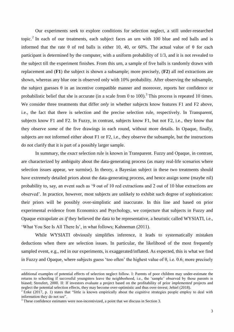
Our experiments seek to explore conditions for selection neglect, a still under-researched

topic.2 In each of our treatments, each subject faces an urn with 100 blue and red balls and is

informed that the rate θ of red balls is either 10, 40, or 60%. The actual value of θ for each

participant is determined by the computer, with a uniform probability of 1/3, and it is not revealed to

the subject till the experiment finishes. From this urn, a sample of five balls is randomly drawn with

replacement and (F1) the subject is shown a subsample; more precisely, (F2) all red extractions are

shown, whereas any blue one is observed only with 10% probability. After observing the subsample,

the subject guesses θ in an incentive compatible manner and moreover, reports her confidence or

probabilistic belief that she is accurate (in a scale from 0 to 100).3 This process is repeated 10 times.

We consider three treatments that differ only in whether subjects know features F1 and F2 above,

i.e., the fact that there is selection and the precise selection rule, respectively. In Transparent,

subjects know F1 and F2. In Fuzzy, in contrast, subjects know F1, but not F2, i.e., they know that

they observe some of the five drawings in each round, without more details. In Opaque, finally,

subjects are not informed either about F1 or F2, i.e., they observe the subsample, but the instructions

do not clarify that it is part of a possibly larger sample.

In summary, the exact selection rule is known in Transparent. Fuzzy and Opaque, in contrast,

are characterized by ambiguity about the data-generating process (as many real-life scenarios where

selection issues appear, we surmise). In theory, a Bayesian subject in these two treatments should

have extremely detailed priors about the data-generating process, and hence assign some (maybe nil)

probability to, say, an event such as ‘9 out of 10 red extractions and 2 out of 10 blue extractions are

observed’. In practice, however, most subjects are unlikely to exhibit such degree of sophistication:

their priors will be possibly over-simplistic and inaccurate. In this line and based on prior

experimental evidence from Economics and Psychology, we conjecture that subjects in Fuzzy and

Opaque extrapolate as if they believed the data to be representative, a heuristic called WYSIATI, i.e.,

‘What You See Is All There Is’, in what follows; Kahneman (2011).

While WYSIATI obviously simplifies inference, it leads to systematically mistaken

deductions when there are selection issues. In particular, the likelihood of the most frequently

sampled event, e.g., red in our experiments, is exaggerated/inflated. As expected, this is what we find

in Fuzzy and Opaque, where subjects guess ‘too often’ the highest value of θ, i.e. 0.6; more precisely

additional examples of potential effects of selection neglect follow. I: Parents of poor children may under-estimate the

returns to schooling if successful youngsters leave the neighborhood, i.e., the ‘sample’ observed by those parents is

biased; Streufert, 2000. II: If investors evaluate a project based on the profitability of prior implemented projects and

neglect the potential selection effects, they may become over-optimistic and thus over-invest; Jehiel (2018). 2 Enke (2017, p. 1) states that “little is known empirically about the cognitive strategies people employ to deal with

information they do not see”. 3 These confidence estimates were non-incentivized, a point that we discuss in Section 3.

4

with a frequency higher than 1/3, that is, the actual frequency. Indeed, the frequency of guess θ = 0.6

respectively equals 53.1 and 56.6% in Fuzzy and Opaque, with an increasing tendency over time.

Further, we analyze the individual guesses in detail and observe that the heuristic exactly predicts

around 60% of them in Fuzzy and Opaque, whereas the remaining guesses can be partly rationalized

if we posit that subjects follow WYSIATI with some error. For instance, deviations from the

heuristic are most likely (i) among subjects who are least attentive or (ii) in borderline situations, that

is, when the frequency observed in the subsample is close to the threshold that, in theory, predicts a

change in the guess. Point (i) is maybe noticeable: Most attentive subjects act more in line with

WYSIATI. As a result, they are more likely to have inflated beliefs in Fuzzy and Opaque. In

contrast, inflation does not depend on the subject’s major or statistical background. In summary,

most subjects seem to use WYSIATI, even the statistically sophisticated, but the least attentive ones

commit more ‘mistakes’ in their application.

We also explore three factors or circumstances that might attenuate selection neglect or at

least induce a more cautious attitude among the subjects. Our first conjecture is that selection neglect

should be greatly reduced if inference is relatively easy and the selection rule non-ambiguous. In this

line, we find little inflation, if any, in Transparent, where subjects know the specific sampling

procedure. Indeed, the overall frequency of guess θ = 0.6 equals 31.3%, close to the actual frequency

of 1/3. This suggests that subjects, even those lacking basic statistical knowledge, understand

sampling biases and how to infer when there are (simple) selection issues. A second conjecture is

that subjects in Fuzzy and Opaque might become more circumspect about their guesses as the size of

the sample increases and patently signals a selection problem. While such circumspection need not

induce them to change their guesses, it seems a prerequisite for such change.4 In all three treatments,

however, average confidence increases as the experiment proceeds and subjects become more

experienced. This is perhaps striking, as subjects face a paradox: They often observe samples where

most (or all) balls are red, but at the same time know that 60% is the largest possible rate of red balls.

As the experiment proceeds, indeed, the mean and median probability of obtaining the subjects’

observed sample under the assumption of random sampling tends to zero in any treatment. In spite of

this, subjects do not become more circumspect, as we have said, Note as well that average

confidence is not significantly different across treatments: Subjects are equally certain in the

ambiguous treatments as in the treatment with full information about the selection rule. A third

conjecture, finally, is that selection neglect occurs when subjects fail to realize that there might be

4 Think also of a scenario in which people can obtain (at a cost) additional information about the selection procedure,

reducing the ambiguity in this regard. If they have little doubts about the accuracy of their guesses, they are unlikely to

search for that information.

5

sampling biases. This could be the case in Opaque, except maybe in the last periods, where the

samples observed include so many red balls. In Fuzzy, however, the instructions clearly indicate the

existence of a selection issue and, given the unbalanced samples typically observed by the subjects,

they should be aware that the sample could be non-random. Hence, subjects should be less confident

in Fuzzy than in Opaque. This is not what we find, though. To prevent selection neglect, therefore, it

is apparently not enough to warn people that there could be sampling biases.

The rest of the paper is organized as follows. The next section describes the experimental

design. Section 3 starts with some summary results and then presents and discusses a theoretical

framework that formalizes the heuristic. It also offers an individual analysis of our data, guided by

such framework. Section 4 surveys previous literature connected with our findings. Finally, Section 5

concludes by discussing some potential ideas for future research.

2. Experimental design and procedures

This simple experiment consists of three treatments. In Transparent, each subject is assigned

a ‘virtual urn’ with 100 balls, blue and red. The rate θ of red balls is either 0.1, 0.4, or 0.6 ‒i.e., there

can be 10, 40 or 60 red balls in the urn. Each subject is uninformed of the actual value of θ in her urn

but knows that it is randomly determined: the probability of having 10, 40, or 60 red balls in the urn

is 1/3. The computer then extracts five random draws with replacement from the subject’s urn, and

some of these five draws are shown to the subject (no feedback on order of extraction is provided).

Disclosure depends on the color of the draw: all red balls extracted are observed, whereas each blue

extraction is observed with a probability of 10%. After the disclosed draws (if any) are presented, the

subject must provide a guess θ ∊ {0.1, 0.4, 0.6} of the rate θ in her urn, reporting as well her

subjective probability (confidence hereafter) that such guess is correct, on a scale from 0 to 100,

where 0 means that the guess is surely false and 100 that the guess is surely correct. The above-

described process consisting in (1) five extractions, (2) partial revelation, and (3) joint elicitation of

the subject’s guess and confidence is repeated 10 periods, always with the same rate θ, so that at the

end of the experiment a total of 50 balls are extracted from the urn of each participant. Subjects get

always feedback about the previously observed extractions. At the end of the session, one of the 10

periods is randomly chosen for payment. Each subject is paid 10 euros if her guess in the chosen

period coincides with θ.5 All previous information is common knowledge in Transparent.

5 Subjects received no prize for the accuracy of their confidence levels. While incentivizing beliefs about the co-players’

choices in VCM games seems to make the estimations more accurate (e.g. Gächter and Renner 2010), when measuring

confidence in one’s own performance this effect is ambiguous (e.g. Keren 1991). As we discuss later, moreover, our

interest is not on the accuracy of the subjects’ stated confidence, but on its tendency along the 10 periods (e.g., increasing

6

The Fuzzy treatment is identical to Transparent except that subjects are not informed about

the disclosure rules ‒i.e., that all red draws are shown whereas blue ones are shown with probability

0.1. Subjects know that some of the five draws are not observed, but do not know exactly which

ones. In turn, the Opaque treatment only differs from Fuzzy in that subjects are not informed that

some extractions are possibly not shown, i.e., they are only told that they will observe in each period

a variable number of extractions (between 0 and 5). In summary, Transparent differs from the other

two treatments in the level of ambiguity regarding the data-generation process. In turn, the key

difference between Fuzzy and Opaque lies in how obvious a selection issue is.

The experiment was programmed and conducted with the experimental software z-Tree

(Fischbacher, 2007). There was one session per treatment, conducted at LINEEX (University of

Valencia) in March and April of 2017, with 62 participants per session. Subjects were undergraduate

students without previous experience in experiments on statistical inference. Each subject

participated in just one treatment.6 Upon arrival, subjects received written instructions that described

the inference problem (see Appendix I). Subjects could read the instructions at their own pace and

their questions were answered privately. Understanding of the rules was checked with a control

questionnaire that all subjects had to answer correctly before they could start with the decision

problem (Appendix I provides examples of some interfaces).

Once subjects’ guesses had been elicited in the 10 periods, participants answered a brief

questionnaire to assess personal and socio-demographic characteristics (gender, age, major,

religiosity, and political ideology), risk attitudes,7

and cognitive abilities ‒using an expanded

cognitive reflection test (henceforth CRT; Frederick, 2005). We also asked them the number of

semesters that they had studied statistics or econometrics at the university. After the CRT, moreover,

subjects performed a memory task: A list with 15 randomly generated, four-digit numbers was

presented on screen and they were given 60 seconds to memorize as many as possible. In the next

screen they had to answer correctly two simple arithmetic problems: (a) (14x10) – 25 = ? and (b)

(5x8) + 39 = ? Only when they did so, a new screen allowed them to introduce the recalled numbers,

ordered as they wished. They had 60 seconds for that and were paid 1 Euro for each correct number.

After answering a new set of five ‘current affairs’ questions and questions regarding the use of the

media (which are analyzed in a follow-up paper), each subject had one guess randomly selected for

payment, and was paid in private. Each session lasted approximately 75 minutes, and on average

or decreasing) and how it compares across treatments. In this regard, we had no reason to believe that our results would

be different had subjects been incentivized. 6 Participants are not significantly different across treatments in their socio-demographic characteristics.

7 Subjects faced the choice between lottery A with prizes 2 and 1.6 Euros and lottery B with prizes 3.85 and 0.1 Euros,

with equal probabilities of the larger and lower prize across lotteries. Letting P denote the probability of the larger prize,

they had to indicate the threshold value of P such that they always preferred B to A, on a scale from 0 to 100.

7

subjects earned 14.3 Euros in Control, 13.7 in Fuzzy, and 12.7 in Opaque, including a show-up fee of

6 Euros.

3. Results

This section is organized as follows. In 3.1, we report some aggregated data on subjects’

guesses and degree of confidence. As we explain, the data hints that subjects do not consider the

possibility of sampling biases when there is ambiguity in this respect, inflating their guesses as a

result. The WYSIATI heuristic/principle is then formally presented in 3.2, while we check its

empirical relevance at an individual level in section 3.3. In section 3.4 we use a regression analysis to

provide more details on the factors that affect the subjects’ guesses and level of confidence, as well

as on the probability of deviation from what the principle predicts.

3.1 Summary of results

Our three treatments correspond to three different situations. In Transparent, the exact

selection rule is known. In Fuzzy and Opaque, subjects do not know the rule, and based on the

existing literature we conjecture them to infer as if there was no selection issue, even when it should

be obvious in Fuzzy that the sample might not be representative.8 As a consequence, subjects in

Fuzzy and Opaque should equate the frequencies of observation and occurrence. Since most of these

subjects observe a high frequency of red, their predictions should be ‘inflated’ with respect to those

in Transparent. More precisely, we have the following hypothesis.

Hypothesis 1 (H1): In comparison with Transparent, subjects in Fuzzy and Opaque tend to

guess more frequently the highest rate, i.e., 0.6. Hence, the average elicited guess is biased upwards

in these treatments. On the other hand, the distribution of guesses in these two treatments are not

different.

Figure 1: Distribution of guesses of the number of red balls in each treatment

Figure 1 above plots the distribution of guesses in the three treatments (N = 620 in each

treatment; Tables A, B, and C in Appendix II offer more disaggregated data). Consistent with H1, the

8 Recall that in Fuzzy subjects know that five balls are extracted but that not necessarily all five are disclosed.

N=167

N=259

N=194

01

02

03

04

05

06

0

Pe

rce

nta

ge (

%)

10 40 60

Transparent

N=95

N=196

N=329

01

02

03

04

05

06

0

Pe

rce

nta

ge (

%)

10 40 60

Fuzzy

N=69

N=200

N=351

01

02

03

04

05

06

0

Pe

rce

nta

ge (

%)

10 40 60

Opaque

8

distribution is similar in Fuzzy and Opaque but quite different in Transparent. Indeed, considering

individual-averaged guesses, a Mann-Whitney test of the equality of distributions in Fuzzy and

Opaque does not reject the null hypothesis (p-value = 0.438). In contrast, the p-values for the

comparison of the distributions of guesses in Transparent vs. Fuzzy and Transparent vs. Opaque are

both lower than 0.001. If in addition we compare the frequency of choosing 0.6 under the three

treatments, we find that the null hypothesis of equal frequencies is not rejected when we compare

Fuzzy and Opaque (p-value = 0.514), but it is rejected at any significance level if we compare

Transparent and Fuzzy or Transparent and Opaque (p-value < 0.001 in both cases). Note also that the

frequency of choice of the highest rate, i.e., 0.6, is significantly larger than 1/3 in Fuzzy and Opaque,

but not in Transparent, evidence again that beliefs are ‘inflated’ in the former treatments.9

The ‘inflation’ of the beliefs is not only persistent; in fact, it becomes more acute in the latter

periods. As our regression analysis confirms in section 3.4, in effect, the rate of choice of 0.6 in

treatments Fuzzy and Opaque increases as the experiment proceeds,10

a phenomenon that is not

observed in Transparent. Because of these dynamics, there is an increasing difference between the

average beliefs in Fuzzy and Opaque and that in Transparent; see Table 1 below, which indicates the

average guess in any period and treatment. In fact, the average guess in Transparent tends to

decrease, and coincidentally reaches in the last period a value that coincides with the expected

number of red balls in the urn, that is, (10+40+60)/3 ≈ 36.6.

Treatment

Period Transparent Fuzzy Opaque TOTAL

1 42.1 40.6 45.6 42.8

2 39.4 41.9 44.4 41.9

3 35.5 45.0 47.3 42.6

4 39.7 43.9 52.9 45.5

5 36.9 45.6 47.7 43.4

6 37.6 48.9 48.1 44.8

7 39.2 46.0 48.5 44.6

8 37.9 47.9 47.9 44.6

9 36.9 49.4 47.6 44.6

10 36.6 51.0 49.8 45.8

TOTAL 38.2 46.0 48.0 44.1

Table 1: Average guess across treatments and periods

9 In a one-sided test where the null hypothesis states that the frequency of the guess 0.6 equals 1/3, whereas the

alternative assumes it to be larger than 1/3, the p-value is 0.716 in Transparent, but it is lower than 0.001 in Fuzzy and

Opaque. All these tests have been performed with individual-averaged data. 10

In this respect, we speculate that the inflation in Fuzzy and Opaque would have grown bigger if subjects had seen, say,

60 extractions instead of 50.

9

Result 1 (inflation): Subjects report inflated guesses in Fuzzy and Opaque and inflation

increases as the experiment proceeds. The distributions of guesses in these two treatments are not

significantly different. There is no such inflation in Transparent.

It must be noticed that the inflated guesses in Fuzzy and Opaque are not innocuous, but

possibly lead to worse outcomes. In effect, since the guesses that do not coincide with the true

number of red balls get no prize if they are selected for payment, and the inflation makes less likely

that a guess coincides with the actual target, we predict that the share of subjects who get the prize is

larger in Transparent than in Fuzzy and Opaque. In this line, this share respectively equals 54.8% in

Transparent, 46.8% in Fuzzy and 38.7% in Opaque.

We turn now our attention to the level of confidence that subjects report after each of the 10

guesses, that is, the probability with which they believe their guess to be correct. Figure 2 depicts the

average level of confidence in each period of each treatment (see Table D in Appendix II for the

precise figures). We make three remarks. First, we observe very minor differences across treatments;

something to be later confirmed by our regression analysis in section 3.4. This is consistent with the

hypothesis that subjects in Fuzzy and Opaque operate as if there were no sampling biases, i.e., as if

the data was reliable. In effect, if they had some doubts in this respect their average levels of

confidence should be lower than the average level in Transparent, where subjects have all the

relevant information. Clearly, this is not what Figure 2 shows.

Figure 2: Average confidence per treatment and period

For the second remark, consider a subject in Fuzzy or Opaque who believes a priori, that

sampling biases could occur with some probability; more precisely, biases favoring the observation

of red balls. If she observes period after period that most extractions are red, her priors that the

sample is non-representative should be reinforced. In effect, since at most 60% of the balls are red,

50

55

60

65

70

75

1 2 3 4 5 6 7 8 9 10Period

Transparent Fuzzy Opaque

Subject's confidence (0-100)

10

the observation of a sample in which the empirical frequency is close to 1 should increase the

posterior that the sample is not representative. Given this uncertainty, the subject should arguably

state decreasing levels of confidence ‒particularly in the last periods, where the sample size is larger.

This should not take place in Transparent. Therefore, we should observe an increasing difference

between Transparent and the other treatments as the experiment progresses. Yet Figure 2 clearly

indicates this not to be the case. In other words: In a scenario characterized by an ambiguous

selection problem, people do not become more circumspect about their inferences when the evidence

strongly suggests such a problem.

In any treatment, third, average confidence increases as the experiment progresses; this is a

significant effect, as our analysis in section 3.4 confirms. This increase in confidence has at least two

possible interpretations: (i) As the sample size grows, subjects gain confidence, and (ii) as subjects

play more periods, they understand better the statistical problem and hence consider their guesses

more accurate. Yet the evidence seems relatively more consistent with account (ii). In effect, recall

that subjects ‘observe’ all extractions in Transparent. This means that the sample size tends to be

substantially larger there, particularly in the last periods. Consequently, subjects in Transparent

should be more confident, especially in the last period. As we said before, this is not what we see in

Figure 2. We explore in more detail this question in section 3.4 but note that the relative insensitivity

to sample sizes that subjects seem to exhibit in their inferences, is something in line with abundant

prior evidence; e.g., Tversky and Kahneman (1971).

Result 2 (confidence): The average subject is similarly confident in the accuracy of her

guess at any given period in all treatments, i.e., irrespectively of the information she has about the

reliability of the data. Average confidence increases as the experiment progresses.

3.2 Selection neglect: An analytical framework

We here formalize the WYSIATI heuristic, while the next section explores its empirical

relevance at an individual level. Specifically, consider a random sample extracted from a statistical

population with two subsets, Blue (B) and Red (R). This sampling defines an i.i.d. signal S, taking on

a value of either B or R. The frequency of red individuals in the population equals θ ∊ [0, 1], this

being as well the rate at which random variable S is generated ‒i.e., Prob(S = R) = θ.

An agent called Adam knows that any rate θi ∊ [0, 1] in some set Θ = {θ1, θ2,…, θN} is a

potential value of θ, but does not know the actual θ. Further, he knows the value of some realizations

of S, but possibly not all. In other words, Adam does not observe some individuals in case they are

randomly extracted. In this line, let οR ∊ [0, 1] denote the fraction of extractions with value R that are

known/observed (out of θi ∊ Θ) if signal S is generated ‒the observable fraction οB of individuals in

11

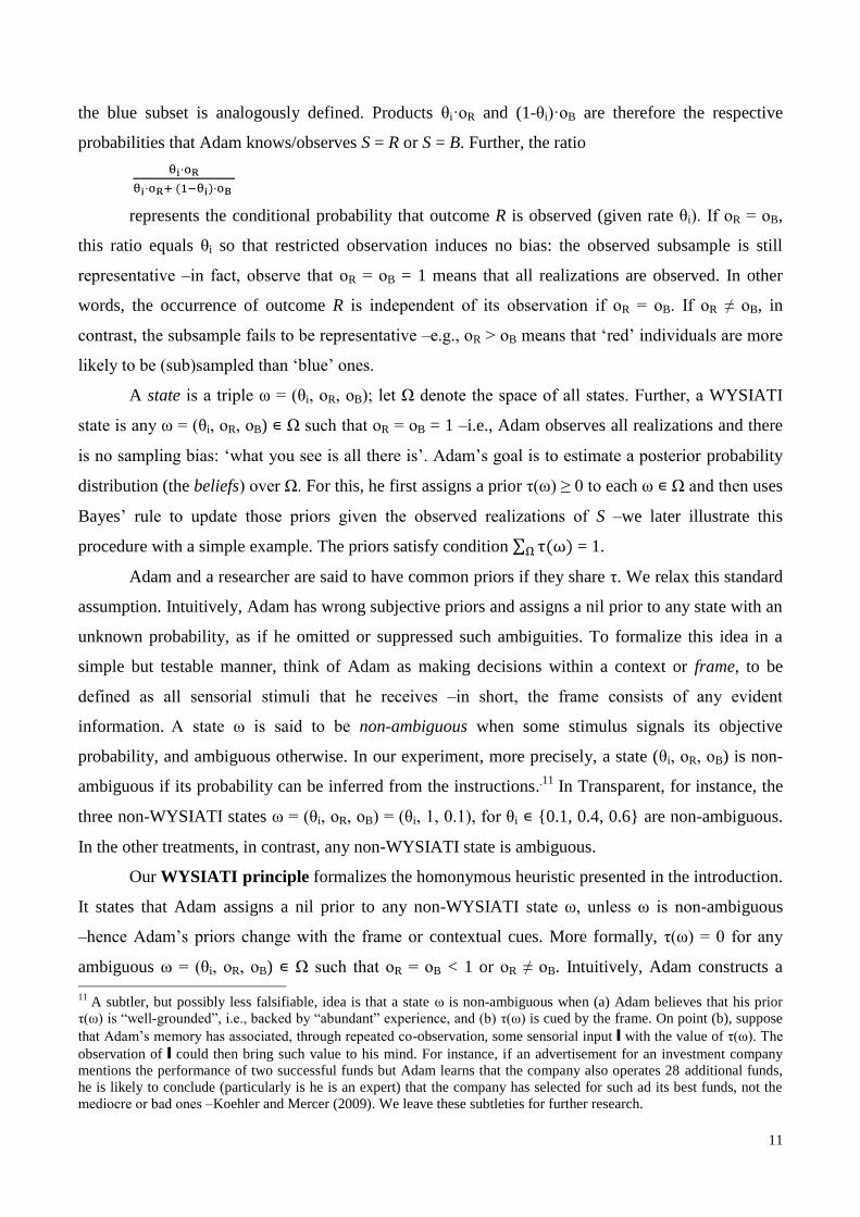
the blue subset is analogously defined. Products θi·οR and (1-θi)·οB are therefore the respective

probabilities that Adam knows/observes S = R or S = B. Further, the ratio

represents the conditional probability that outcome R is observed (given rate θi). If οR = οB,

this ratio equals θi so that restricted observation induces no bias: the observed subsample is still

representative ‒in fact, observe that οR = οB = 1 means that all realizations are observed. In other

words, the occurrence of outcome R is independent of its observation if οR = οB. If οR ≠ οB, in

contrast, the subsample fails to be representative ‒e.g., οR > οB means that ‘red’ individuals are more

likely to be (sub)sampled than ‘blue’ ones.

A state is a triple ω = (θi, οR, οB); let Ω denote the space of all states. Further, a WYSIATI

state is any ω = (θi, οR, οB) ∊ Ω such that οR = οB = 1 ‒i.e., Adam observes all realizations and there

is no sampling bias: ‘what you see is all there is’. Adam’s goal is to estimate a posterior probability

distribution (the beliefs) over Ω. For this, he first assigns a prior τ(ω) ≥ 0 to each ω ∊ Ω and then uses

Bayes’ rule to update those priors given the observed realizations of S ‒we later illustrate this

procedure with a simple example. The priors satisfy condition = 1.

Adam and a researcher are said to have common priors if they share τ. We relax this standard

assumption. Intuitively, Adam has wrong subjective priors and assigns a nil prior to any state with an

unknown probability, as if he omitted or suppressed such ambiguities. To formalize this idea in a

simple but testable manner, think of Adam as making decisions within a context or frame, to be

defined as all sensorial stimuli that he receives ‒in short, the frame consists of any evident

information. A state ω is said to be non-ambiguous when some stimulus signals its objective

probability, and ambiguous otherwise. In our experiment, more precisely, a state (θi, οR, οB) is non-

ambiguous if its probability can be inferred from the instructions..11 In Transparent, for instance, the

three non-WYSIATI states ω = (θi, οR, οB) = (θi, 1, 0.1), for θi ∊ {0.1, 0.4, 0.6} are non-ambiguous.

In the other treatments, in contrast, any non-WYSIATI state is ambiguous.

Our WYSIATI principle formalizes the homonymous heuristic presented in the introduction.

It states that Adam assigns a nil prior to any non-WYSIATI state ω, unless ω is non-ambiguous

‒hence Adam’s priors change with the frame or contextual cues. More formally, τ(ω) = 0 for any

ambiguous ω = (θi, οR, οB) ∊ Ω such that οR = οB < 1 or οR ≠ οB. Intuitively, Adam constructs a 11

A subtler, but possibly less falsifiable, idea is that a state ω is non-ambiguous when (a) Adam believes that his prior

τ(ω) is “well-grounded”, i.e., backed by “abundant” experience, and (b) τ(ω) is cued by the frame. On point (b), suppose

that Adam’s memory has associated, through repeated co-observation, some sensorial input I with the value of τ(ω). The

observation of I could then bring such value to his mind. For instance, if an advertisement for an investment company

mentions the performance of two successful funds but Adam learns that the company also operates 28 additional funds,

he is likely to conclude (particularly is he is an expert) that the company has selected for such ad its best funds, not the

mediocre or bad ones ‒Koehler and Mercer (2009). We leave these subtleties for further research.

12

parsimonious representation of the world that is as coherent as possible with the frame. Any

ambiguous selection rule is excluded from such representation.12

To facilitate the test of the

principle, we finally assume that Adam’s priors over the remaining states are a re-normalization of

the researcher’s priors over the set of all states that are either WYSIATI or non-ambiguous.

3.3 Exploring individual guesses: A test of the WYSIATI principle

We first apply the principle to Transparent, where subjects know that parameters οR and οB

equal respectively 1 and 0.1. Since there is no uncertainty on οR and οB, the prior τ(ω) of any feasible

state ω = (θi, οR, οB) is simply denoted as τ(θi). As subjects also know the total number of balls drawn

from the urn up to any period (k = 5, 10,…, 50) and the total number of red draws (call it r), applying

the principle is relatively straightforward. Given that the signal follows a binomial distribution and

the number of blue balls actually extracted happens to be equal to k – r, posterior beliefs for rate θi

given history H = (k, r) are:

p(θi|H) =

=

, (1)

where the last equality follows from the fact that the priors are uniform. At any period, the

optimal guess of θ is the mode of the posterior distribution over Θ = {0.1, 0.4, 0.6}, as this estimate

maximizes the probability that the 10 Euros prize is won if the period is finally selected for payment.

Let f = r/k denote the (actual) empirical frequency of red balls given a sample with a total of k

extractions. If we compare expression (1) for the three possible values of rate θi ∊ {0.1, 0.4, 0.6} and

do some algebra, we have that the optimal guess is θi = 0.1 if f ≤ 0.226, θi = 0.4 if 0.226 < f ≤ 0.5,

and θi = 0.6 if 0.5 ≤ f. In effect, it suffices to check that

p(θi = 0.6 |H) ≥ p(θi = 0.4 |H) ↔ ≥ ⇒ f ≥ 5

and

p(θi = 0.1 |H) ≥ p(θi = 0.4 |H) ↔ ≥ ⇒ f ≤

≈ 22 2

As a rule of thumb, the predicted guess in any period is the rate in Θ closest to frequency f,

except when 0.226 < f ≤ 0.25, in which case θi = 0.4 is optimal. Further, there are two modes when f

= 0.5.13

Figure 3 summarizes the discussion.

12

Adam’s story excludes sampling biases (unless they are non-ambiguous) but also the possibility that oR = oB < 1, i.e.,

no sampling bias but only a strict subsample is observed. This is just for simplicity: Given our focus, the key assumption

is that Adam operates as if the sample were random.

13 Properly speaking, there are also two modes in the hypothetical case that f =

. We omit this possibility because

the probability that the frequency of red takes exactly such value in a subject’s sample is basically nil. Note also that the

threshold of 0.226 that we consider in Figure 3 is slightly lower than this theoretical one. If f = 0.226, therefore, the

subject should unequivocally guess a rate of 0.1.

13

Figure 3: Optimal guesses conditional on empirical frequency of red

We turn now to individual predictions in Fuzzy and Opaque, where the exact sampling

procedure is ambiguous. By the WYSIATI principle, agents infer as if οR = οB = 1 was certain.14

If

the subject has observed b and r blue and red balls, respectively, the principle says that he will be

positive that the number of extractions is b + r. Note that b + r ≤ k, as some balls might not be

selected out of the sample. Given the observed history Ho = (b, r), therefore, he will compute his

posterior beliefs as follows (as before, the last equality follows from the fact that priors are uniform):

p(θi| Ho) =

=

Again, her optimal guess coincides with the mode of this posterior distribution. Let fo = r /(b

+ r) denote the observed empirical frequency of red balls given history Ho, that is, the percentage of

red in the observed subsample. Following an analogous argument as in Transparent, the mode of the

posterior distribution is θi = 0.1 if fo ≤ 0.226, θi = 0.4 if 0.226 < fo ≤ 0.5, and θi = 0.6 if 0.5 ≤ fo.

Further, there are also two modes (θi = 0.4, 0.6) when fo = 0.5, and we add a case that did not appear

before: When a subject has observed no ball in period t and the precedent ones, the original, uniform

priors are unchanged and hence any rate is an optimal guess (θi = 0.1, 0.4, 0.6).15

Leaving aside the

few exceptions noted, in any case, the rule of thumb is that the rate chosen should be closest to fo.

Hypothesis 2 summarizes our predictions for the different treatments:

Hypothesis 2 (H2): In Transparent, guesses of the rate of red balls depend on the actual

frequency of red extractions, while in Fuzzy and Opaque they track the observed frequency of red

balls.

14

Some readers might think that an alternative way to test the WYSIATI principle is to elicit the subject’s priors that the

data is representative or reliable. While this provides a direct test of the principle, taken literally, we would rather insist

on conceiving the principle in “as if” terms. In other words, we do not rule out that subjects in Opaque and particularly in

Fuzzy actually consider the possibility that there are sampling biases, potentially of many different shapes. Since they do

not know the specific selection rule, however, they find difficult to mentally operate in such an uncertain scenario, and

hence simplify matters, i.e., suppress ambiguity, inferring as if there were no selection issues. 15

This case did not appear in Transparent because, when the subjects observe no balls in a period there, they are assumed

to know that the five extractions of that period are actually blue-colored.

Optimal

guess θi = 0.1 θi = 0.4 θi = 0.6

θi = 0.4, 0.6

f = 0.5 f = 1 f = 0 f = 0.226

θi = 0.1

14

Evidence: Table 2 below indicates the percentage of guesses consistent with H2 in each

period of each treatment.16

As we can see, H2 overall predicts 57, 58.9, and 62% of the guesses in

Transparent, Fuzzy, and Opaque, respectively. We note as well that the fit of the model does not

improve as the experiment proceeds in Transparent, but there is some positive trend in Fuzzy and

Opaque; the regression analysis below provides more details on this

Treatment

Period Transparent Fuzzy Opaque TOTAL

1 58.1 48.4 66.1 57.5

2 59.7 51.6 46.8 52.7

3 58.1 53.2 50.0 53.8

4 50.0 54.8 74.2 59.7

5 64.5 58.1 56.5 59.7

6 51.6 61.3 61.3 58.1

7 53.2 59.7 66.1 59.7

8 51.6 62.9 67.7 60.8

9 62.9 69.4 62.9 65.1

10 59.7 69.4 67.7 65.6

TOTAL 57.0 58.9 62.0 59.2

Table 2: Frequency of choices consistent with the WYSIATI principle

Result 3: In Transparent, 57% of the guesses are predicted by the heuristic, with no

significant improvement along time. In Fuzzy and Opaque, around 60% of the subjects guess in

accordance with the heuristic, with a positive trend over time.

Note that the principle is equally successful across treatments: Leaving aside some small

differences, around 60% of the subjects follow the observed frequency in the three treatments. This

is somehow reassuring, as we do not predict a different rate of success in any treatment. Since the

explanatory power of the principle is not extremely high, however, one might wonder whether the

choices left unexplained follow a very different logic than the one suggested by the principle.

For some reasons, we think that this is not the case: Many deviations from the principle can

be rationalized as simple mistakes. On one hand, we will show in section 3.4 that deviations are most

likely when the inference problem is arguably most difficult, that is, when the empirical frequency is

close to the thresholds indicated in Figure 3. Further, people scoring lower on the CRT, who possibly

pay less attention to the information in the screens, instructions, etc., are significantly more likely to

16

For more detailed data, Table A in Appendix II displays the number of subjects choosing each rate θi in Transparent,

for any history ‒determined by period and empirical frequency of red, presented in intervals [0, 0.226], (0.226, 0.5], (0.5,

1]. In addition, Tables B and C in Appendix II respectively display the number of subjects in Fuzzy and Opaque choosing

each rate θi, conditional on the observed history.

15

deviate.17

On the other hand, we have evidence that some subjects apply the logic of the principle in

a (cognitively) ‘myopic’ manner. In other words, their guesses in period t are based only on the

treatment-relevant frequency in that period. This group contrasts with the possibly more attentive,

‘non-myopic’ subjects, who consider the frequency across t and all prior periods (if any). In short,

myopic subjects follow the WYSIATI principle imperfectly, focusing on recent evidence, whereas

non-myopic ones estimate in absolute accordance with our predictions. This extension of our theory

is called henceforth the ‘two-types’ model.

To explore the empirical accuracy of this extension, we first conduct a classification analysis

of the subjects in each treatment. We compute, for each subject, the number of guesses consistent

with the WYSIATI principle according to the treatment-relevant frequency in (i) the most recent

period and (ii) across all periods. A subject is classified as “myopic” if the number of predicted

guesses is higher in case (i). The percentage of myopic subjects is 38.8, 38.7 and 35.5% in

Transparent, Fuzzy and Opaque, respectively. Using this classification, we then compute the share of

guesses that are explained by the two-types model in any treatment and period. This data can be

found in Table 3 below, which is to be contrasted with Table 2 above, showing the empirical

relevance of our ‘single-type’ theory presented in Section 2.

Frequency (%)

Period Transparent Fuzzy Opaque TOTAL

1 58.1 48.4 66.1 57.5

2 62.9 58.1 59.7 60.2

3 66.1 64.5 61.3 64.0

4 59.7 64.5 74.2 66.1

5 72.6 75.8 66.1 71.5

6 56.5 77.4 72.6 68.8

7 69.4 75.8 69.4 71.5

8 66.1 72.6 75.8 71.5

9 64.5 75.8 71.0 70.4

10 72.6 75.8 74.2 74.2

TOTAL 64.8 68.9 69.0 67.6

Table 3: Frequency of guesses consistent with the two-types model

In percentage points, the two-types model explains 7.8, 10, and 7 p.p. more than the single-

type model in Transparent, Fuzzy, and Opaque, respectively. Overall, the improvement in all

17

Psychologists often contend that the CRT score is a good measure of how willing someone is to meditate on a problem

(Kahneman, 2011). In each CRT problem, there is one specious answer, salient and therefore tempting, but wrong. For

instance, in the question “A bat and a ball together cost $1.10, and the bat costs $1.00 more than the ball: how much does

the ball cost?” the trap answer is $0.10. Participants must therefore think carefully enough to avoid the trap.

16

treatments equals 8.4 percentage points. Although these figures are not very large, they provide

further evidence that a significant part of the guesses unexplained by the WYSIATI principle can be

rationalized by introducing small adjustments, in particular, allowing for mistakes.

We have also investigated the possibility that some subjects in Transparent behave as those in

Fuzzy or Opaque, i.e., without considering the non-observed blue extractions. For each subject and

period, more precisely, we computed whether the subject's guess is more consistent with the

predictions from the theory taking the actual (Transparent) or the observed (Fuzzy and Opaque)

empirical frequency of red balls. We found that 16.3% of the subjects’ guesses in Transparent are

better explained by assuming that they track the observed, instead of the actual, frequency.

Result 4 (deviations): A significant share of the deviations from the WYSIATI principle

seems to be caused by subjects’ mistakes, including considering only the current period sample (not

the whole one).

3.4 Further tests of the WYSIATI principle: Regression analysis

In this section, we perform some regression analyses to explain the subjects’ guesses, the

probability of deviation from the WYSIATI principle, and the subjects’ degree of confidence in

terms of characteristics of the experimental design, as well as individual characteristics. There are

variables that are common in all models, such as the dynamics of the experiment, and specific

variables that are related to the observed frequency of red balls and the classification of subjects as

myopic or non-myopic. In Table 4 the dependent variable is the subject’s guess about the number of

red balls, with values {10, 40, 60}. We use an ordered probit model to estimate the probability of

choosing each of these alternatives. We have included, as explanatory variables, the period, the

observed frequency of red balls in the current period and in all prior periods, the interaction of these

frequencies with the variable that indicates the subject’s type (myopic vs. non-myopic) and some

controls related to individual characteristics. To simplify, we only report the average partial effects

of each variable on the probability of a guess of 60.18

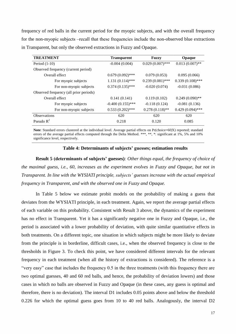
Our results confirm prior findings. Regarding the evolution of the experiment, captured by

the variable “period”, we find no significant effect in Transparent, but a positive and significant

effect in Fuzzy and Opaque, in line with Result 1 above. In these two treatments, it is more likely a

guess of 60 red balls as the experiment evolves. Confirming the results from our two-types model

analysis, in addition, the likelihood of a guess of 60 co-moves in all treatments with the empirical

18

Since we estimate an ordered probit model, the sign of the partial effects of each variable on the probability of a guess

of 10 is, by construction, the opposite of the sign of the partial effect on the probability of a guess of 60. Results on the

average partial effects on the probability of every outcome, as well as the estimated coefficients from the ordered probit

model (instead of average partial effects) are available from the authors upon request.

17

frequency of red balls in the current period for the myopic subjects, and with the overall frequency

for the non-myopic subjects ‒recall that these frequencies include the non-observed blue extractions

in Transparent, but only the observed extractions in Fuzzy and Opaque.

TREATMENT Transparent Fuzzy Opaque

Period (1-10) -0.004 (0.004) 0.029 (0.007)*** 0.013 (0.007)**

Observed frequency (current period)

Overall effect 0.679 (0.092)*** 0.079 (0.053) 0.095 (0.066)

For myopic subjects 1.131 (0.114)*** 0.239 (0.081)*** 0.339 (0.108)***

For non-myopic subjects 0.374 (0.135)*** -0.020 (0.074) -0.031 (0.086)

Observed frequency (all prior periods)

Overall effect 0.141 (0.141) 0.119 (0.102) 0.249 (0.090)**

For myopic subjects -0.400 (0.155)*** -0.118 (0.124) -0.081 (0.136)

For non-myopic subjects 0.533 (0.202)*** 0.278 (0.118)** 0.429 (0.094)***

Observations 620 620 620

Pseudo R2

0.218 0.120 0.085

Note: Standard errors clustered at the individual level. Average partial effects on Pr(choice=60|X) reported; standard

errors of the average partial effects computed through the Delta Method. ***, **, *: significant at 1%, 5% and 10%

significance level, respectively.

Table 4: Determinants of subjects’ guesses; estimation results

Result 5 (determinants of subjects’ guesses): Other things equal, the frequency of choice of

the maximal guess, i.e., 60, increases as the experiment evolves in Fuzzy and Opaque, but not in

Transparent. In line with the WYSIATI principle, subjects’ guesses increase with the actual empirical

frequency in Transparent, and with the observed one in Fuzzy and Opaque.

In Table 5 below we estimate probit models on the probability of making a guess that

deviates from the WYSIATI principle, in each treatment. Again, we report the average partial effects

of each variable on this probability. Consistent with Result 3 above, the dynamics of the experiment

has no effect in Transparent. Yet it has a significantly negative one in Fuzzy and Opaque, i.e., the

period is associated with a lower probability of deviation, with quite similar quantitative effects in

both treatments. On a different topic, one situation in which subjects might be more likely to deviate

from the principle is in borderline, difficult cases, i.e., when the observed frequency is close to the

thresholds in Figure 3. To check this point, we have considered different intervals for the relevant

frequency in each treatment (when all the history of extractions is considered). The reference is a

“very easy” case that includes the frequency 0.5 in the three treatments (with this frequency there are

two optimal guesses, 40 and 60 red balls, and hence, the probability of deviation lowers) and those

cases in which no balls are observed in Fuzzy and Opaque (in these cases, any guess is optimal and

therefore, there is no deviation). The interval D1 includes 0.05 points above and below the threshold

0.226 for which the optimal guess goes from 10 to 40 red balls. Analogously, the interval D2

18

includes 0.05 points above and below the threshold 0.5 (without including 0.5), for which the

optimal guess goes from 40 to 60 red balls. These two intervals D1 and D2 around the threshold

values can be arguably considered as difficult ones. The rest of the unit interval is considered as an

“easy” case, intermediate between the “very easy” one and the frequencies around the thresholds

(without 0.5, that is included in the “very easy” case). Focusing on the Transparent treatment, it is

clear that the probability of deviation is higher when the frequency is around the thresholds, even in

the easy interval. When the frequency is in this interval (with respect to the reference category) the

probability of deviation increases around 35 p.p. The effect is much higher when the frequency is

around the thresholds, 56 p.p. in D1 and 46 p.p. in D2.19

In Fuzzy and Opaque there is not enough

variability to estimate all these effects, more specifically those of D1 and D2. However, we can

compare what happens in the “very easy” and the “easy” case. We find that the probability of

deviation increases around 30 p.p. in the latter (compared to the former one).

TREATMENT Transparent Fuzzy Opaque

Period (1-10) 0.001 (0.007) -0.030 (0.007)*** -0.018 (0.006)***

Frequency

interval

Easy (rest of the unit interval) 0.349 (0.067)*** 0.344 (0.046)*** 0.274 (0.049)***

D1: 0.226±0.05 0.556 (0.095)*** ---- ----

D2: 0.5±0.05, excluding 0.5 0.459 (0.099)*** ---- ----

Myopic subject 0.199 (0.055)*** 0.215 (0.062)*** 0.262 (0.065)***

Number of correct answers in CRT -0.108 (0.024)*** -0.101 (0.030)*** -0.040 (0.031)

Observations 620 619 617

Pseudo R2 0.135 0.165 0.101

Note: Standard errors clustered at the individual level. (a) Average partial effects reported; (b) Standard errors of the

average partial effects computed through the Delta Method. In Fuzzy and Opaque, some observations in D1 are lost

due to lack of variability of the dependent variable; further, there are no observations in D2. The reference interval is

the “very easy” one, that is, freq = 0.5 and “no balls seen”. ***, **, *: significant at 1%, 5% and 10% significance

level, respectively.

Table 5: Determinants of a deviation from the WYSIATI principle; estimation results

We also report how the subject’s type is associated with the probability of deviation from the

model in 3.2. As expected by construction, for myopic subjects this probability is higher (around 20

p.p.) than for the non-myopic ones, with some slight differences across treatments. Concerning the

CRT, a good performance is associated with a lower probability of deviation. This is found in all

three treatments, with a slightly higher effect in Transparent and Fuzzy; the effect in Opaque is non-

significant at the usual levels, but the p-value is not too high, 0.198.

Result 6 (Determinants of a deviation): Deviations from the principle are more likely (i)

among the least reflective subjects, (ii) among the myopic subjects, (iii) and when the inference

problem is more complex. This suggests again that many of the deviations are the result of applying

19

We have tested, from the estimated probit model, whether there is a statistical difference between the coefficients of

the frequency intervals D1 and D2 in Transparent. We have not found evidence of such difference (p-value: 0.325).

19

the principle with some error, not the result of a substantially different logic of choice. The

probability of deviation in Fuzzy and Opaque (but not in Transparent) is significantly reduced as

more and more periods are played.

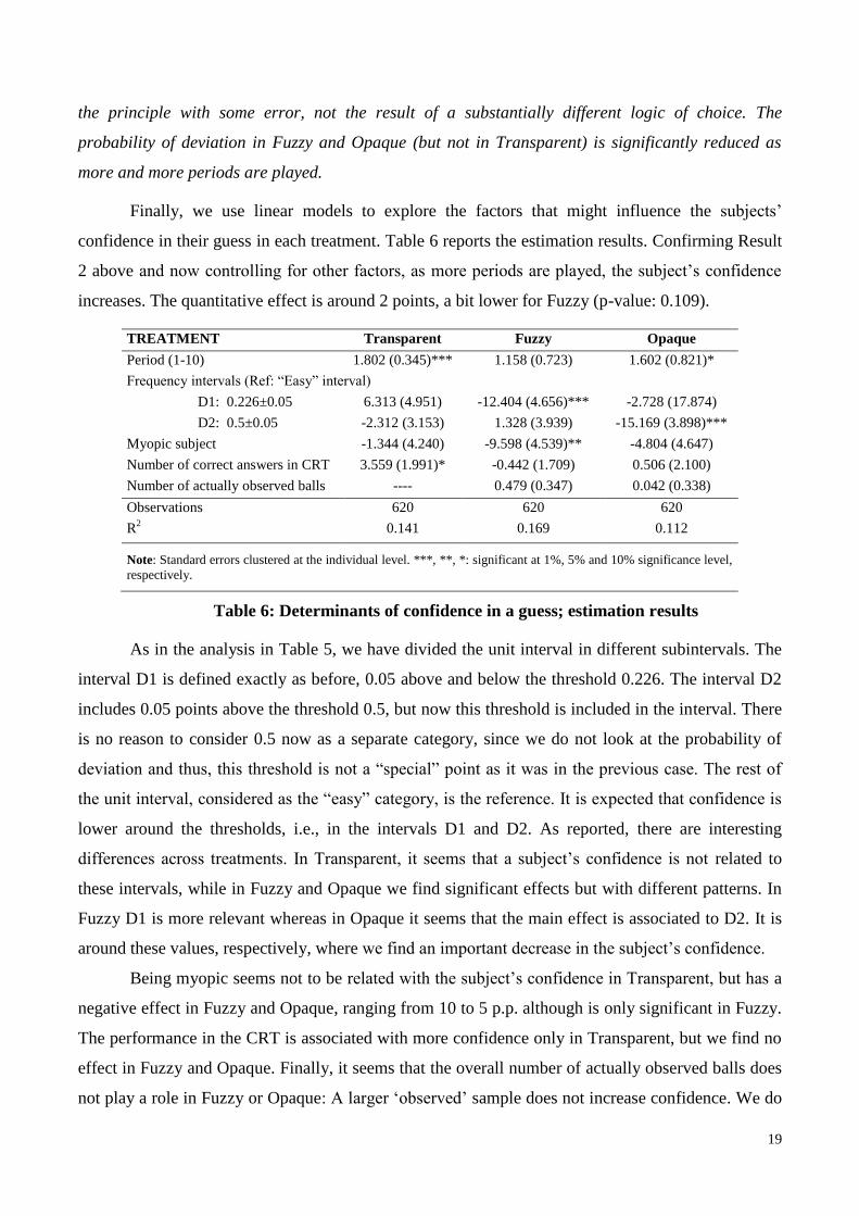
Finally, we use linear models to explore the factors that might influence the subjects’

confidence in their guess in each treatment. Table 6 reports the estimation results. Confirming Result

2 above and now controlling for other factors, as more periods are played, the subject’s confidence

increases. The quantitative effect is around 2 points, a bit lower for Fuzzy (p-value: 0.109).

TREATMENT Transparent Fuzzy Opaque

Period (1-10) 1.802 (0.345)*** 1.158 (0.723) 1.602 (0.821)*

Frequency intervals (Ref: “Easy” interval)

D1: 0.226±0.05 6.313 (4.951) -12.404 (4.656)*** -2.728 (17.874)

D2: 0.5±0.05 -2.312 (3.153) 1.328 (3.939) -15.169 (3.898)***

Myopic subject -1.344 (4.240) -9.598 (4.539)** -4.804 (4.647)

Number of correct answers in CRT 3.559 (1.991)* -0.442 (1.709) 0.506 (2.100)

Number of actually observed balls ---- 0.479 (0.347) 0.042 (0.338)

Observations 620 620 620

R2 0.141 0.169 0.112

Note: Standard errors clustered at the individual level. ***, **, *: significant at 1%, 5% and 10% significance level,

respectively.

Table 6: Determinants of confidence in a guess; estimation results

As in the analysis in Table 5, we have divided the unit interval in different subintervals. The

interval D1 is defined exactly as before, 0.05 above and below the threshold 0.226. The interval D2

includes 0.05 points above the threshold 0.5, but now this threshold is included in the interval. There

is no reason to consider 0.5 now as a separate category, since we do not look at the probability of

deviation and thus, this threshold is not a “special” point as it was in the previous case. The rest of

the unit interval, considered as the “easy” category, is the reference. It is expected that confidence is

lower around the thresholds, i.e., in the intervals D1 and D2. As reported, there are interesting

differences across treatments. In Transparent, it seems that a subject’s confidence is not related to

these intervals, while in Fuzzy and Opaque we find significant effects but with different patterns. In

Fuzzy D1 is more relevant whereas in Opaque it seems that the main effect is associated to D2. It is

around these values, respectively, where we find an important decrease in the subject’s confidence.

Being myopic seems not to be related with the subject’s confidence in Transparent, but has a

negative effect in Fuzzy and Opaque, ranging from 10 to 5 p.p. although is only significant in Fuzzy.

The performance in the CRT is associated with more confidence only in Transparent, but we find no

effect in Fuzzy and Opaque. Finally, it seems that the overall number of actually observed balls does

not play a role in Fuzzy or Opaque: A larger ‘observed’ sample does not increase confidence. We do

20

not check for this ‘sample size’ effect in Transparent because subjects should know there the number

of actual extractions (including observed and unobserved ones). Since this number is given by 5·t,

where t is the period, there is perfect collinearity between the period and the size of the sample.

Result 7 (confidence): As the number of periods increases, the confidence of the subjects

regarding the accuracy of their guess increases in all treatments, although not always significantly.

This effect does not seem to be due to an increase in the sample size. On the other hand, in Fuzzy and

Opaque, subjects’ confidence decreases significantly in some difficult intervals.

To finish, we note that we have controlled in all previous estimations for individual

characteristics, such as gender, age, major, knowledge of statistics, risk aversion, and a measure of

the subject’s memory (how many 4-digit numbers shown during 60 seconds they are able to

remember). The most interesting result regarding individual characteristics is that, other things equal,

being a male increases the confidence on the guess made, around 6 and 7 p.p. respectively in

Transparent (significant at 10%) and Fuzzy (significant at 12%). This result is in line with a vast

literature that confirms that men in general are more (over)confident than women (e.g., Fellner and

Maciejovsky, 2007; Niederle and Vesterlund, 2007), and even more when it is about some

mathematics-related task (e.g. Dahlbom et al. 2010, Jacobsson et al. 2013). Regarding other

variables, we find that in Transparent, age slightly decreases the probability of deviation and

increases the confidence on the guess made (both results significant at 5%). We also stress that the

number of semesters that a subject has studied statistics or econometrics at the university and her/his

major has no systematic effect. Studying Engineering or Sciences, for instance, does not make a

subject less likely to have inflated beliefs in Fuzzy and Opaque (i.e., more likely to deviate from our

model’s prediction).

4. Related literature

Our paper is closely related to a psychological literature claiming that people often neglect

selection issues. For instance, subjects in Nisbett and Borgida (1975) equated some observed,

extreme behavior to the modal one for the population, both when the sampling procedure was

unspecified, i.e., ambiguous, or explicitly described as random. Hamill et al. (1980) similarly report

that subjects’ attitudes toward welfare recipients ‒i.e., their maturity, capacity for hard-working,

etc.‒ were equally influenced by exposure to a single case, both when subjects were told that the case

was highly (i) typical or (ii) atypical. Several factors could explain selection neglect in these studies.

For instance, Hamill et al. (1980, p. 587) contend that “the vivid sample information probably serves

to call up information of a similar nature from memory […]. These memories then would be

21

disproportionately available when judgments are later made about the population”. In our

experiment, in contrast, memory biases arguably play little (if any) role, e.g., subjects are always

given feedback about prior extractions, they have the instructions available, and it is unlikely that

any of the extractions observed are cognitively more “available”, as they only differ in their color.

Relatedly, we control for the subjects’ priors and the information that they use in their inferences so

that we can provide evidence on the extent to which individuals follow the WYSIATI principle.

This study is also related to an emerging empirical literature in Economics studying belief

updating when people do not observe some signal realizations. In general terms, our contribution to

this literature is to provide detailed evidence at an individual level in line with the WYSIATI

principle, documenting as well how ambiguity affects selection neglect, even when both the evidence

accumulated by the subjects and contextual cues strongly suggest the existence of selection biases.

We also explore the reasons why people sometimes deviate from the principle, finding that they can

be partly attributed to mistakes. Among the most closely related papers, Koehler and Mercer (2009)

offer evidence that companies selectively (and possibly strategically) advertise their better-

performing stock mutual funds. Nonetheless, investors (both experts and novices) respond to mutual

fund advertisements as if such data were unselected, in line with the WYSIATI principle. The

authors’ preferred explanation is that people do not automatically think about sampling matters

unless the exact data selection process is made transparent or cued. Our findings add further evidence

in this line from a controlled experimental settings, indicating moreover that the mere accumulation

of evidence signaling a selection issue is not enough to make people doubt about their inferences. In

turn, the experiment in Enke (2017) has a random variable which is uniformly distributed over the

set {50, 70, 90, 110, 130, 150}. Out of six realizations, subjects first observe one of them and then

also those above (below) 100, depending on whether the first observed outcome is above (below)

100 as well. Based on such evidence, subjects must infer the average outcome. Akin to our

Transparent treatment, therefore, there is a sampling bias, but subjects know the selection rule ‒in

our terminology, the state ω is non-ambiguous. Even in this case, interestingly, a substantial share of

the subjects infers as if they fully neglected the non-observed outcomes, i.e., in line with the

WYSIATI principle, thus suggesting that the scope of the problem is even broader than what our

parsimonious framework concedes. Similarly, but in the context of an investment experiment, Barron

et al. (2019) find evidence for selection neglect in a treatment in which subjects know the data

generating process. The results from these two latter studies, therefore, contrast with the evidence

from Transparent, where subjects fully account for the sampling bias. Hence, we complement this

perspective by showing that, keeping complexity constant, the ambiguity of the specific selection

rule is a factor behind selection neglect; we expand on this issue in the conclusion.

22

We also contribute to a literature on quasi-Bayesian inference, where agents misread the

world due to cognitive limitations, but are then assumed to operate as Bayesians given this

misreading. A strand of this literature, including Barberis et al. (1998), Rabin and Schrag (1999),

Mullainathan (2002), Rabin (2002), and Benjamin et al. (2016), explore inference when agents

misread or misremember the signals they observe. In another strand, more closely related to our

paper, agents do not misinterpret the signal, but have a simplified representation of the state space.

For instance, Gennaioli and Shleifer (2010) and Bordalo et al. (2016) consider a world defined by

several dimensions. Some of them are fixed by the available data and hypothesis that the agent wants

to evaluate, but others are uncertain. Agents simplify the world by focusing on the “stereotypical"

values of these residual dimensions, that is, those values that are frequently observed in a world in

which the target hypothesis is true (as well as the data), but uncommon when the complementary

hypothesis is true. In our framework, for instance, the residual dimensions of state ω = (θi, οR, οB) are

possibly the pair οR, οB, while any hypothesis refers to the rate θ. A difference with Gennaioli and

Shleifer (2010) is that the WYSIATI principle does not mean that people focus on the stereotypical

values of οR and οB, but on those that are either non-ambiguous (given the frame) or simplify most

inference (i.e., assuming that there are no sampling biases; οR = οB = 1). The idea that people have

reduced representations of the world also relates our paper to the behavioral literature on inattention

–see Gabaix (2019) for a nice review. Another related issue is correlation neglect ‒DeMarzo et al.

2003, Glaeser and Sunstein, 2009; Levy and Razin, 2015; Ortoleva and Snowberg, 2015. This is the

idea that, when people exchange ideas with others, they tend not to realize how often others have

observed the same evidence as them –e.g., the same news. Since WYSIATI implies a sampling-bias

neglect (unless the selection rule is non-ambiguous), it implies as well that agents will discount the

possibility that they mostly interact with people who have similar evidence.

There is a growing literature that studies how others’ private information affects players (and

their decisions) in strategic settings, mainly in auctions and voting. In strategic interactions, (naïve)

players may underestimate selection effects or more precisely the correlation between other players’

actions and the information they have. In a common value auction, a naïve winner does not fully

appreciate that, for her bid to win, other bidders must have more negative private information than

her own and hence make lower bids. Since the average bidder is estimating correctly, the failure to

anticipate the correlation between bids and private information leads the winner to overbid relative to

the equilibrium prediction, succumbing to the so-called winner’s curse. Kagel and Levin (1986), Holt

and Sherman (1994), Eyster and Rabin (2005), and more recently Araujo et al (2018) have, among

others, studied implications of such correlation neglect in markets affected by adverse selection. In

addition, Esponda and Vespa (2014) find in a simple voting situation that the majority of the subjects

23

fail to be strategic, but this mistake is primarily driven by the fact that these subjects are unable to

extract information from hypothetical events. This failure turns out to be fairly robust to experience,

feedback, and hints about pivotality. Similarly, Esponda and Vespa (2018) find that subjects are

unable to account optimally for endogenous sample selection (caused by private information of other

players). They find that subjects respond to observed data, but they pay no attention to the possibility

that this data may be biased. Jin, Luca and Martin (2018) study an information disclosure game.

Besides finding a high overall disclosure rate among senders, they observe that receivers are not

sufficiently skeptical about undisclosed information, as they (mistakenly) think that non-disclosed

states are higher than they are in reality. While these articles consider selection neglect (and its

consequences in strategic settings), we explore several conditions that might affect the prevalence of

this phenomenon, including ambiguity, the evidence accumulated, and explicit contextual cues.

5. Conclusion

Our claim is that, when faced with some evidence, people often update their beliefs as if they

faced a representative sample of the population. The main reason is that data-generating procedures

are often ambiguous or uncertain. Under these conditions, people simplify matters and infer as if

there was no sampling bias; a heuristic we call the WYSIATI principle. As Kahneman (2011, p. 114)

states, “System 1 is not prone to doubt” As a result, people tend to equate the frequency of

observation and occurrence of the target event when there are ambiguous selection problems.

The problem of course appears if the two frequencies are actually different. Consider for

instance journalism. If rare or shocking events (‘man bites dog’) receive disproportionate coverage

while ordinary, ‘nice’ events are not considered newsworthy, readers may conclude that extreme and

terrible events are more common than they are in reality. The press can in that manner feed

pessimism, leading people (even experts) to inflate the probability of a massive stock-market crash,

the danger of terrorist attacks or airplane crashes, the crime rate, or the prevalence of genocide and

war in the world. In this line, a survey conducted by the end of 2015 revealed that majorities in 15

countries around the world believed that the world is getting worse ‒in the US, for instance, 65%

thought so, and only 6% responded that the world is getting better.20

Partly motivated by these phenomena, we explore the empirical relevance of the WYSIATI

principle, and find that it replicates a substantial share of the subject’s individual guesses. Further,

many of the guesses not explained by the heuristic seem to be caused by simple mistakes, not by a

different logic of inference. In this line, the likelihood of a deviation increases as subjects are less

reflective, apparently put more emphasis on recent observations (rather than taking into account the 20

See https://yougov.co.uk/news/2016/01/05/chinese-people-are-most-optimistic-world/. Indonesia and China were the

only two countries surveyed where majorities did not respond that the world outlook was worsening.

24

whole sample) or have borderline evidence. The results across treatments suggest moreover that

ambiguity strongly influences the prevalence of selection neglect, even when people become

experienced in the inference problem at hand and the context hints that the evidence observed might

be selective. The alternative theory that subjects cannot make correct inferences is at odds with the

data from Transparent, where inflation is absent and the average guess converges over time to the

Bayesian prediction. The idea that subjects are unaware of potential sampling biases seems in turn

incoherent with the fact that subjects in Fuzzy are not more cautious or conservative than those in

Opaque: the inflation rate and the average confidence are basically the same in these two treatments.

Finally, subjects do not seem to operate with complex priors on the data-generating process, because

their guesses and confidence levels in Fuzzy and Opaque increase as the experiment proceeds.

Our results indicate that inflation can be a lasting phenomenon, but also one that can be

alleviated if the exact selection rule is non-ambiguous. Alternatively, the objective probability of the

target event could be given. Following with our prior example, the media might reduce the inflation

generated by their emphasis on tragedy and calamity if, together with the news on some uncommon

event, they reported empirical frequencies of that type of events. In our setting at least, people can

adjust their beliefs in a Bayesian manner (although perhaps not perfectly) if they get sufficiently

detailed evidence.

There are a number of issues that we leave for future research, from which we mention three.

One refers to group polarization –e.g., Sunstein, 2001. This phenomenon is indeed a multifaceted

one, but we conjecture that part of the problem is that groups do not realize that the information they

receive is not sufficiently ‘varied’, i.e., depicting different points of view and a representative sample

of data. While polarization is possibly compounded by the fact that groups do not trust those sources

of information that contradict their worldview, it seems to us that it would be alleviated if agents

were aware of the potential biases in the samples they observe. Another issue is that selection neglect

possibly implies a neglect as well of the statistical causes of the bias. For instance, do people tend to

under-estimate the prevalence of (a) selection effects and (b) biased reporting of evidence by others,

either intentional or unintentional? To illustrate point (a), suppose that, for whatever reasons, female

scientists appear less frequently than their male peers in textbooks, magazines, and TV shows for

children. If children ignore the potential selection effects causing female scientists to be less

numerous than their male peers, they will think as if ‘what they see is all there is’, hence affecting

their stereotypical perceptions of who is (and possibly who can be) a scientist.21

21

Children’s drawings of scientists may reflect stereotypical perceptions. The meta‐analysis of 5 decades of

Draw‐A‐Scientist studies in Miller et al. (in press) finds that American children draw female scientists more often in later

25

A final topic is sampling-bias neglect in complex statistical problems: multiple signals, some

of them time-varying absence of feedback, etc. Compared to the relative simplicity of Fuzzy and

Opaque, our impression is that, other things equal, inflation should be even more severe and lasting

in complex environments. This point is maybe related to the evidence from Enke (2017) and Barron

et al. (2019), who find selection neglect even when the selection rule is known. In contrast, we

observe no sampling bias neglect in Transparent. While explaining these differences across the

studies is out of the scope of this paper, one could argue that inference in Enke (2017) and Barron et

al. (2019) is cognitively more demanding than in Transparent. Perhaps people (or at least some

types) follow the WYSIATI principle in non-ambiguous but computationally complex scenarios, as

their limited attention is focused on the ensuing computations. More research is indeed warranted.

decades, maybe due to an increasingly more balanced depiction in the mass media. In the 1960s and 1970s, 99.4% of the

kids did not draw female researchers; today around one in three does it.

26

Bibliography

Araujo, F.A., Wang, S.W. and A.J. Wilson (2018): “The Times They Are A-

Changing: Dynamic Adverse Selection in the Laboratory”, working paper.

Barberá, P. (2014): “Birds of the Same Feather Tweet Together: Bayesian Ideal

Point Estimation Using Twitter Data.” Political Analysis, 23, pp. 76-91.

Barberis, N., A. Shleifer, and R. W. Vishny (1998): “A Model of Investor

Sentiment.” Journal of Financial Economics, 49, pp. 307-343.

Barron, K., S. Huck, and P. Jehiel (2019). “Everyday econometricians: Selection

neglect and overoptimism when learning from others”, WZB Discussion Paper, No. SP

II 2019-301, Wissenschaftszentrum Berlin für Sozialforschung (WZB), Berlin.

Benjamin, D. J., M. Rabin, and C. Raymond (2016): “A Model of Non-Belief in

the Law of Large Numbers.” Journal of the European Economics Association, 14(2),

pp. 515-544.

Bordalo, P., K. Coffman, N. Gennaioli and A. Shleifer (2016): “Stereotypes.”

The Quarterly Journal of Economics, 131(4), pp. 1753–1794

Dahlbom, L., A. Jakobsson, N. Jakobsson, and A. Kotsadam (2010): “Gender

and Overconfidence: Are Girls Really Overconfident?” Applied Economics Letters, 18,

pp. 325-327

DeMarzo, P., D. Vayanos, D and J. Zwiebel (2003): “Persuasion Bias, Social

Influence and Uni-Dimensional Opinions.” Quarterly Journal of Economics, 118(3), pp.

909-968

Enke, B. (2017): “What You See Is All There Is.” Working paper.

http://dx.doi.org/10.2139/ssrn.2691907

Esponda, I. and E. Vespa (2014): “Hypothetical Thinking and Information

Extraction in the Laboratory”, American Economic Journal: Microeconomics, 6(4), pp.

180-202.

Esponda, I. and E. Vespa (2018): “Endogenous Sample Selection: A Laboratory

Study”, Quantitative Economics, 9, pp. 183-216.

Eyster, E., and M. Rabin (2005): “Cursed Equilibrium.” Econometrica, 73(5),

pp. 1623–72

Fiedler, K. (2000): “Beware of samples! A cognitive-ecological sampling

approach to judgment biases”, Psychological Review, 107, pp. 659-676

27

Fellner, G. and B. Maciejovsky (2007): “Risk Attitude and Market Behavior:

Evidence from Experimental Asset Markets”. Journal of Economic Psychology, 28, pp.

338-350

Fischbacher, U. (2007): “Z-Tree: Zurich Toolbox for Ready-Made Economic

Experiments.” Experimental Economics, 10(2), pp. 171-178

Frederick, S. (2005): “Cognitive Reflection and Decision Making”. Journal of

Economic Perspectives, 19(4), pp. 25-42

Gabaix, X. (2019). Behavioral Inattention, in Handbook of Behavioral

Economics, Vol. 2, eds. D. Bernheim, S. DellaVigna, and D. Laibson, Elsevier.

Gächter, S. and E. Renner (2010): “The Effects of (Incentivized) Belief

Elicitation in Public Goods Experiments”. Experimental Economics, 13, pp. 364-377

Gennaioli, N. and A. Shleifer (2010): “What Comes to Mind.” The Quarterly

Journal of Economics, 125(4), pp. 1399-1433

Glaeser, E. L., and C. R. Sunstein (2009): “Extremism and Social Learning.”

Journal of Legal Analysis, 1(1), pp. 263–324

Hamill, R.; T. D. Wilson, and R. E. Nisbett (1980). “Insensitivity to Sample

Bias: Generalizing from Atypical Cases.” Journal of Personality and Social

Psychology, 39(4), pp. 578-589

Holt, C.A. and R. Sherman (1994): “The Loser’s Curse.” American Economic

Review, 84, pp. 642–652

Jacobsson, N., Levin, M., and Kotsadam, A. (2013): “Gender and

Overconfidence: Effects of Context, Gendered Stereotypes, and Peer Group”. Advances

in Applied Sociology, 3, pp. 137-141

Jehiel, P. (2018): “Investment Strategy and Selection Bias: An Equilibrium

Perspective on Overoptimism”. American Economic Review, 108(6), pp. 1582-97.

Jin, G.Z., Luca, M. and D. Martin (2018): “Is No News (Perceived As) Bad

News? An Experimental Investigation of Information Disclosure”, NBER Working

Paper 21099.

Kagel, J. H., and D. Levin (1986): “The Winner’s Curse and Public Information

in Common Value Auctions.” American Economic Review, 76, pp. 894–920

Kahneman, D. (2011): Thinking, Fast and Slow. Farrar, Straus & Giroux.

Keren, G. (1991): “Calibration and Probability Judgements: Conceptual and

Methodological Issues.” Acta Psychologica, 77, pp. 217–273

28

Koehler, J. J., and M. Mercer (2009): “Selection Neglect in Mutual Fund

Advertisements.” Management Science, 55(7), pp. 1107–21.

Levy, G., and R. Razin (2015): “Correlation Neglect, Voting Behavior, and

Information Aggregation.” American Economic Review, 105(4), pp. 1634-45

Levy, G., and R. Razin (2019): “Echo Chambers and Their Effects on Economic

and Political Outcomes.” Annual Review of Economics, 11

Miller, D. I., Nolla, K. M., Eagly, A. H. and Uttal, D. H. (2018): “The

Development of Children's Gender‐Science Stereotypes: A Meta‐analysis of 5 Decades

of U.S. Draw‐A‐Scientist Studies.” Child Development, 89(6), pp. 1943-1955

Mullainathan, S. (2002): “A Memory-Based Model of Bounded Rationality.”

The Quarterly Journal of Economics, 117(3), pp. 735–774

Mullainathan, S. and A. Shleifer (2005): “The Market for News.” American

Economic Review, 95(4), pp. 1031–1053

Niederle, M. and Vesterlund, L. (2007): “Do Women Shy Away from

Competition? Do Men Compete Too Much?” The Quarterly Journal of Economics, 122,

pp. 1067-1101

Nisbett, R. E., and E. Borgida (1975). “Attribution and the Psychology of

Prediction.” Journal of Personality and Social Psychology, 32, pp. 932-943

Ortoleva, P., and E. Snowberg (2015). “Overconfidence in Political

Behavior.” American Economic Review, 105(2), pp. 504-35.

Rabin, M. (2002): “Inference by Believers in the Law of Small Numbers.”

Quarterly Journal of Economics, 117, pp. 775–816

Rabin, M. and J.L. Schrag (1999): “First Impressions Matter: A Model of

Confirmatory Bias.” The Quarterly Journal of Economics, 114(1), pp. 37–82

Streufert P. (2000): “The Effect of Underclass Social Isolation on Schooling

Choice.” Journal of Public Economic Theory, 2, pp. 461-482

Sunstein, C. A. (2001): Echo Chambers: Bush V. Gore, Impeachment, and

Beyond. Princeton University Press

Tversky, A., and D. Kahneman (1971): “Belief in the Law of Small Numbers.”

Psychological Bulletin, 76, pp. 105-110

29

Appendix I: Instructions for the three treatments

Thank you for participating in this simple experiment on estimation. You will be paid

some money at its end; the precise amount will depend on chance and your decisions.

All decisions are anonymous, that is, the other participants will not get any information

about your decisions, nor do you get any information about the decisions of the others.

Decisions are made via the keyboard of your computer terminal. Read the on-screen

instructions carefully before making any decision; there is no hurry to decide. The

questions are not stated in tricky, confounding terms; choose simply as you prefer.

These instructions meet the basic standards in Experimental Economics; in particular,

all the information that appears in them is true and therefore there is no deception.

Please, do not talk to any other participant. If you do not follow this rule, we will have

to exclude you from the experiment without payment. If you have questions, raise your

hand and we will assist you. The use of calculators and writing tools is not permitted.

Please, switch off your cell phone.

There is a ‘virtual urn’ with 100 balls. Each ball is either blue or red. Let us call R the

number of red balls in the urn. You do not know either R or the number of blue balls

(that is, 100 – R). You only know that R can be equal to 10, 40 or 60 and has been

randomly selected by the computer: The probability of having 10, 40 or 60 red balls in

the urn is 1/3. To understand this with a merely illustrative example, it is as if R had

been determined by rolling a six-sided die, so that if number 1 or 2 had been rolled there

would be 10 red balls (R = 10), if number 3 or 4 had been rolled then R = 40, and if

number 5 or 6 had been rolled then R = 60. The value of R will not change throughout

the experiment.

The experiment consists of 10 periods and your task in each one is to estimate the

number R of red balls that you believe there are in the urn (10, 40, or 60). For this, take

into account two key points. First, the computer will perform [Transparent and Fuzzy:

in each period five] extractions from the urn, randomly and with replacement ‒in other

words: each draw is reintroduced into the urn and can therefore be drawn in the next

Description of the experiment

30

extraction. Each of the 100 balls has the same chance in each extraction. Second, you

will observe in each period the color of a variable number of [Transparent and Fuzzy:

those five] extractions (from 0 to 5). [Transparent: More precisely: If a extracted ball

is red, it will be always shown to you; and if it is blue, it will be shown to you with a

10% probability.]

Once you have performed the 10 estimates, one per period, you will complete an

anonymous questionnaire and afterwards will be paid in private and in cash. Your

payment will include three components. First, 6 Euros for participating in the

experiment. Second, a payment that will depend on the accuracy of your estimates of R.

More precisely, at the end of the session the computer will randomly select one of your

10 estimates and you will win 10 Euros if that estimate exactly matches R, the actual

number of red balls, and zero Euros otherwise. Finally, some questions of the final

questionnaire have an associated prize; we will explain it later. This prize is completely

independent of your estimates of R.

If you have any questions, please raise your hand and we will attend you.

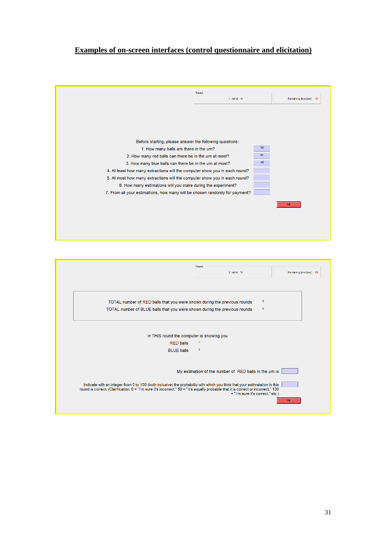
31

Examples of on-screen interfaces (control questionnaire and elicitation)

32

Appendix II: Additional data

Empirical frequency (% red)

Period

[0- 0.226] (0.226- 0.5] (0.5- 1]

Estimation Estimation Estimation

TOTAL 10 40 60 10 40 60 10 40 60

1 10 12 4 2 9 5 1 2 17 62

2 11 3 6 3 14 6 2 7 10 62

3 11 8 2 4 13 2 5 5 12 62

4 8 6 6 5 14 7 1 8 7 62

5 13 8 0 2 18 4 0 8 9 62

6 8 11 1 5 13 6 4 3 11 62

7 10 7 3 3 13 7 2 7 10 62

8 11 7 2 6 9 9 2 5 11 62

9 13 5 2 4 14 5 2 5 12 62

10 11 8 1 5 14 6 3 3 11 62

TOTAL 106 75 27 39 131 57 22 53 110 620

Table A: Number of subjects in Transparent choosing 10/40/60 according to

history

Observed empirical frequency (% red)

Period

[0- 0.226] (0.226- 0.5] (0.5- 1]

Estimation Estimation Estimation

TOTAL 10 40 60 10 40 60 10 40 60

1 3 12 2 0 2 0 7 21 15 62

2 2 3 3 1 3 1 11 15 23 62

3 0 4 0 2 2 2 7 18 27 62

4 1 1 1 2 4 0 9 15 29 62

5 0 1 1 1 3 0 10 13 33 62

6 0 1 1 0 2 2 7 14 35 62

7 0 0 1 2 3 1 9 13 33 62

8 0 0 1 0 5 0 7 15 34 62

9 0 1 0 0 2 0 8 10 41 62

10 0 0 1 1 1 1 5 12 41 62

TOTAL 6 23 11 9 27 7 80 146 311 620

Table B: Number of subjects in Fuzzy choosing 10/40/60 according to observed

history

33

Observed empirical frequency (% red)

Period

[0- 0.226] (0.226- 0.5] (0.5- 1]

Estimation Estimation Estimation

TOTAL 10 40 60 10 40 60 10 40 60

1 5 6 2 0 3 1 2 18 25 62

2 0 1 1 5 2 0 4 23 26 62

3 0 1 0 0 4 2 3 27 25 62

4 0 0 1 0 4 2 2 13 40 62

5 1 0 0 1 2 3 4 21 30 62

6 0 1 0 2 1 0 6 15 37 62

7 1 0 0 0 3 0 6 15 37 62

8 0 1 0 2 1 1 9 8 40 62

9 1 0 0 0 1 1 8 15 36 62

10 -- -- -- 1 1 0 6 13 41 62

TOTAL 8 10 4 11 22 10 50 168 337 620

Note: We report no value (--) if no subject made an estimation for the corresponding history.

Table C: Number of subjects in Opaque choosing 10/40/60 according to observed

history

Treatments

Period TRANSPARENT FUZZY OPAQUE TOTAL

1 57.1 52.4 55.1 54.9

2 57.7 56.4 63.2 59.1

3 60.4 62.5 59.3 60.7

4 59.6 64.9 60.2 61.6

5 66.6 63.2 61.3 63.7

6 67.0 64.5 68.9 66.8

7 66.6 68.2 68.5 67.8

8 68.1 71.2 68.8 69.3

9 71.8 70.2 71.6 71.2

10 70.2 73.0 73.4 72.2

TOTAL 64.5 64.7 65.0 64.7

Table D: Average confidence per treatment and period