SOME DESIGN CONSIDERATIONS FOR THE ESRF UPGRADE PROGRAM EXPERIMENTAL HALL SLAB

D. Martin, ESRF, Grenoble, France

Abstract In 2008, the Council of the European Synchrotron

Radiation Facility (ESRF) launched the ESRF Upgrade Programme 2009-2018, an ambitious ten-year project serving a community of more than 10,000 scientists. Funding for the first phase of the Upgrade (from 2009 to 2015) has been secured to deliver: • eight new beamlines with capabilities unique in the

world; • refurbishment of many existing beamlines to

maintain them at world-class level; • continued world leadership for X-ray beam

availability, stability and brilliance; and, • major new developments in synchrotron radiation

instrumentation. One of the key elements of the Upgrade Program is to

produce nano-sized beams. This will require the construction 120 m and in some cases even 250 m long beamlines. A combination of extended experimental hall and satellite buildings will address this need.

One particularly important issue is the design of the concrete slab that will host these new beamlines. The vibrational stability of the experimental hall slab is a key aspect to in the slab design. However, recent hydrostatic levelling system (HLS*

THE ESRF UPGRADE PROGRAM

) measurements indicate that slab bending movements driven by temperature gradient variations through the slab could also be a very important consideration in beamline stability and performance. This paper presents the measurements that have led to this conclusion.

X-rays are ideally suited for studying matter at the atomic length- and time-scales. Scientists use brilliant beams of X-ray photons for experiments in physics, chemistry, health and life sciences, material sciences, environment, industrial research and increasingly cultural heritage. Demand for high-brilliance X-ray beams is continually growing, with user communities requiring ever increasing levels of performance along with ease of access to and use of the light sources. At the ESRF, the user communities are specifically demanding smaller nanosized beams with higher brilliance, improved facilities on the beamlines and not least more beam time.

The ESRF Upgrade Programme is serving this demand with the additional objective to maintain the ESRF's role as the leading European provider of hard X-ray light. The * An HLS is a tool that is used to precisely monitor vertical motion in sensitive applications.

Upgrade focuses on five core areas of applied and fundamental research: • nanoscience and nanotechnology, • pump-probe experiments and time-resolved

diffraction, • science at extreme conditions, • structural and functional biology and soft matter • X-ray imaging. Producing nano-sized beams needs long beamlines,

which at the ESRF will reach 120 metres and in some cases even 250 metres. A combination of extended experimental hall buildings along with satellite buildings for very long beamlines will address this need. Particular care and effort is being put into the design of the concrete slab to host new beamlines as its stability is pivotal to the beamlines meeting their design performance.†

ESRF EX2 SLAB, LONG BEAMLINES AND TOLERANCES

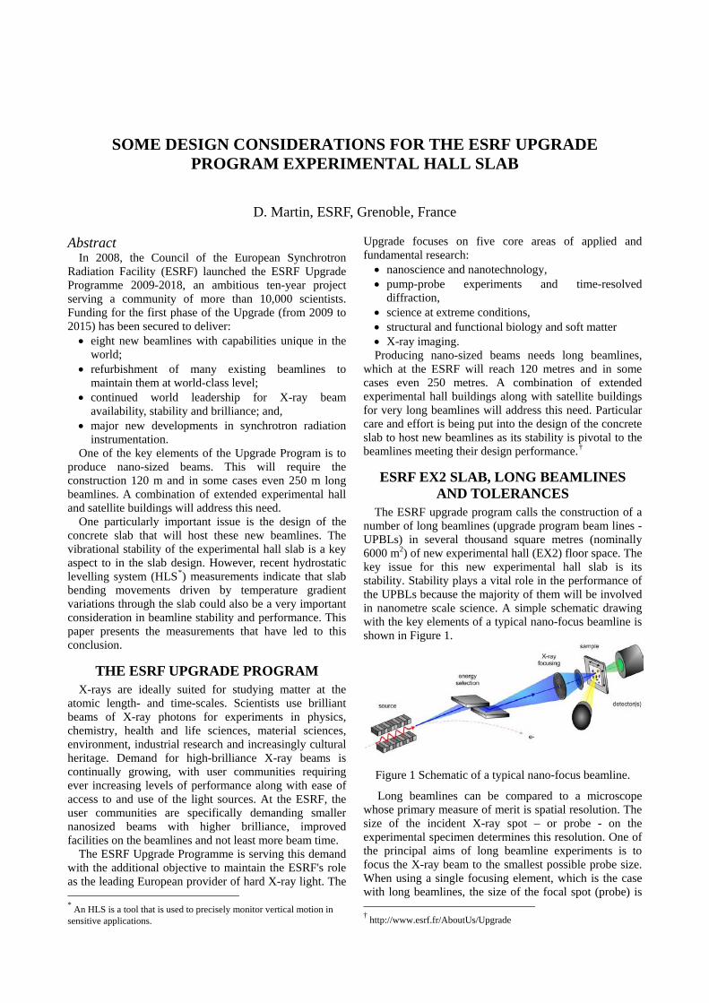
The ESRF upgrade program calls the construction of a number of long beamlines (upgrade program beam lines - UPBLs) in several thousand square metres (nominally 6000 m2) of new experimental hall (EX2) floor space. The key issue for this new experimental hall slab is its stability. Stability plays a vital role in the performance of the UPBLs because the majority of them will be involved in nanometre scale science. A simple schematic drawing with the key elements of a typical nano-focus beamline is shown in Figure 1.

Figure 1 Schematic of a typical nano-focus beamline.

Long beamlines can be compared to a microscope whose primary measure of merit is spatial resolution. The size of the incident X-ray spot – or probe - on the experimental specimen determines this resolution. One of the principal aims of long beamline experiments is to focus the X-ray beam to the smallest possible probe size. When using a single focusing element, which is the case with long beamlines, the size of the focal spot (probe) is † http://www.esrf.fr/AboutUs/Upgrade

limited by the demagnification of the source size and by the diffraction limit (see Figure 2).

Figure 2 The size of the focused X-ray probe spot size depends on: the source size, the distance between the source and the focusing optics p, and the working distance between optics and the experimental sample q. At the ESRF p is nominally 150 m and q is in the order of 0.05 m. The demagnification is therefore q/p=3000-1 giving a theoretical probe size of 10 nm. Actual probe size is expected to be between 20 and 50 nm.

In theory a small beam could be produced using a more complicated optical arrangement on a shorter beamline. In practice, however, the number of X-ray optical components should be restrained whenever possible to minimise beam degradation from sources such as mirror slope errors, absorption in refractive elements, and thermal and vibrational stability. Expected long beamline probe sizes will range between 20 and 50 nm. [1]

Figure 3 Uncertainty due to translation and rotation

errors. Considering the X-ray probe spot size is approximately

50 nm and an acceptable spot drift δ is 10% of its size, or 5 nm, the effect of a pure translation is given by:

5 nm 300015 μm

δ∆ = ×= ×=

z p q

This tolerance must be respected over the time it takes to perform a scan or an experiment. Generally temporal stability is a maximum of 30 minutes. Therefore the vertical stability tolerance, for example, is 15 µm over a period of one half hour. The angular tolerance is given by:

95 10 m 0.05 m100 nrad

θ δ−

∆ =

= ×=

q

Thus the angular or rotational stability tolerance is 100 nrad over a period of one half hour. Uncertainties due to translation and rotation are illustrated in Figure 3.

MEDIUM TO LONG GROUND MOTION AND BACKGROUND CONTEXT

Although slab and ground movements over longer periods than 30 minutes do not influence experimental results, they must be considered in the beamline conception and its long term performance. For example, the ESRF policy has been to maintain the SR machine horizontal. Therefore, if a number of millimetres of vertical uplift or subsidence are expected along the beamline over several years, sufficient stroke must be designed into the instrument alignment mechanisms. A number of systematic site ground motions signatures have been identified at the ESRF and are discussed in [2] and [3].

ESRF long term ground movement between 1997 and 2008 is shown in Figure 4. Several points concerning these movements are worth noting. First, there is a tilting of the entire site in the direction down the Isère river valley (left to right in Figure 4). This is consistent with studies made of the larger scale movement in the region. [4] Second, the centre of the site is sinking. It is caused by the large mass of concrete and earth composing the Booster Synchrotron in this part of the site. Third, there is subsidence around the five story central building (d). Finally, there is also downward movement adjacent to the Drac (a) and Isère (c) rivers and particularly near the part of the site marked (b). This subsidence is due to a combination of: accumulation of silt in the Drac and Isère rivers, and the leeching of small particulate material out of the soil into the large drains that run parallel to the rivers and link at the pumping station located at (b). Because the local water level is above site ground level, continuous pumping keeps the ESRF site dry. The key point is that there is inhomogeneous settlement and that parts of the site are more stable than others.

Referring once again to Figure 4, we remark that ground motion around the SR machine and experimental hall is comparatively small - in the range ±1.5 mm. This is particularly clear in the 3D volumetric plot on the bottom right hand corner of this figure where a ring or crown can be distinguished. Although the mechanism

underlying this is unknown, things that might be considered are ground water and/or precipitation, and the rigidity of the SR tunnel (see Figure 5).

Another very important site movement influence is the periodic purging of the St Egrève dam located downriver of the ESRF. This purge, shown in Figure 6, is typically made in late spring during a period when snow melt runoff combined with heavy precipitation produces high flow that can be used to remove sediment built up in the river. The purging of the St Egrève dam causes permanent systematic uplift and subsidence of the SR machine, and indeed whole ESRF site in the order ±150 µm.

During the construction of the EX2 buildings and experimental hall slab, there will be extensive landscaping and excavation works. An estimated

35,000 m3 of soil will be removed from areas directly adjacent to the existing experimental hall. Because it is planned to operate the ESRF and beamlines during this period, it is important to appreciate the effects of excavation.

During the summer of 2008, 6000 m3 of earth was moved in the centre of the ESRF site for the construction of new office space. Figure 7 shows a net uplift of 225 µm measured by the ESRF SR roof HLS system at its closest point, roughly 60 to 70 m away from these works. The ESRF SR roof HLS is discussed in [5]. Movements at beamline end stations on the existing experimental hall slab located at 30 m from the future excavation areas (see Figure 5) could potentially be larger than those shown in Figure 7.

Figure 4 ESRF long term site movements 1997 to 2008. a) marks the Drac river, b) is the pumping station, c) is the Isère river and d) is the five floor central office building.

Figure 5 Profile showing the existing hall with the SR machine and the new EX2 experimental hall.

Figure 6 The purging of the St Egrève dam downriver of the ESRF causes permanent site uplift and subsidence movements in the order ±150 µm. The top graph shows this movement at one point measured by the HLS installed on the SR tunnel roof. The bottom two photos show the dam and sediment in the Isère River.

Figure 7 Over a relatively short time in summer 2008 roughly 6000 m3 (12 kT) of earth was moved from the site where the buildings now stand to the adjacent areas. A net upward movement of 225 µm was registered on an HLS installed on the SR tunnel roof located roughly 60 to 70 m away.

WHAT CAN BE SAID CONCERNING THE EX2 SLAB TOLERANCES?

At the ESRF a considerable quantity of high quality HLS‡

• 289 sensors on the SR machine quadrupole girders,

data exists over extended periods of time. Among these data are:

• 96 sensors on the SR tunnel roof, • four systems of 6 HLS sensors each on existing long

beamlines, • a system of 29 sensors monitoring the slabs on the

unoccupied beamline BM18, • a system of 17 sensors starting in the SR tunnel

extending to the exterior and running along an existing beamline,

• a system of 8 sensors on the floor and 4 on a mirror installed on a beamline measuring rotational movements of the mirror.

These data can be used to determine both translational and rotational movements on the ESRF site for varying periods of time.

Data analysis and presentation What is the temporal stability of the existing ESRF

floor and how can we estimate it for different time periods? Several possibilities exist. For example, if we have two HLS sensors separated by 10 m taking measurements every five minutes over one year, the difference dH between these two points for the 365×24×12 or 105,120 individual data sets can be calculated. The rotation =dR dH D where D is 10 m, the distance between the two points, can also be estimated if it is appropriate.

Temporal variability can be estimated by taking the difference between measurements made at different times. For example, the difference between all consecutive data points (105,119 values) can be calculated and the standard deviation determined to estimate the variability of dH (ordR ) over 5 minutes. The same can be done for 10 minute (105,118 values), 60 minute (105,059 values), and ten day (90,719 values), or any desired time period. Although this ‡ The ESRF HLS uses a water equi-potential reference surface common to all measuring points. The instruments are composed of two parts: the captor vessels holding he water and linked by a system of pipes, and capacitive probes that measure capacitance which is proportional to the distance between their electrodes and the water surface. When a vessel and probe moves -for example because the support upon which they are installed moves- the distance between the probe and the water surface will increase or decrease. One can measure micrometer level displacements over extensive distances and areas with this system.

simple differencing gives an idea of the variation in the data set for a given time period it doesn’t necessarily represent the variability in dH (or dR ) over the full period being considered.

Another approach is to use all of the data over the given interval. So for the 60 minute interval, we will have 105,059 data sets each with 24×12 or 288 samples for a total of 30,256,992 values. Using the same logic for the ten day period will produce more than 6.27×109 values. Obviously, this will quickly become unwieldy – particularly if we wish to investigate a large number of periods.

A statistically valid and more manageable approach to this problem based on the bootstrap [6] is used here. This approach is outlined below and illustrated in Figure 8:

For a selection of time periods (e.g. 5 minutes, 10 minutes, 30 minutes, 1 hour, …,8 weeks)

a. Select a nominal time period (e.g. 24 hours), b. For a preselected number (e.g. n=50,000) of these

periods sample with replacement§

i. Select at random a starting date and time

from the data set:

0DT , ii. Select the contiguous data set (e.g. for readings

at 5 minute intervals: 24 hours × 12 five minute readings = 288 readings 1 288= iR ) starting with

0DT , iii. Normalize the data by subtracting the first

reading (or mean, or median or some other appropriate value) from the data set dH (i.e.

1= −i idH R R ), iv. Select a random sample 50, jS (e.g. 50 values)

from the data set, c. Concatenate all of the sample data sets 50, 1= j nS

into one vector, d. Form the probability density function (PDF) for

the concatenated data set, e. Calculate an appropriate coverage interval (e.g.

one standard deviation). This technique will produce an estimation of

variability, or uncertainty of the data set which includes both random and systematic effects. For example the effect of continuous subsidence will be similar to cyclical or even very noisy data.

§ With replacement one contiguous data set can potentially be sampled more than once.

Figure 8 Schematic for the sampling process to establish one point in each of the graphs in Figures 10, 15, 19, 22, 25 and 26. Note the resulting PDF is often characterised by ’long tails’.

The resulting data sets often have long tails. Long tails result when a larger share of the population rests within the tail of the probability distribution than observed with a normal or Gaussian distribution. One way to determine a coverage interval for this type of distribution is to fit a t-distribution to it. In the work presented here this is done using the maximum likelihood estimate (MLE) function mle in Matlab with the t Location-Scale Distribution and a coverage factor of 95%.**

** For more information on this function and its parametric form refer to

Translation movements - tolerance 15 µm in 30 minutes

At the ESRF there are four long beamlines equipped with 6 HLS sensors. Figure 9 shows these installations and their situation in relation to the important features discussed above. the Matlab documentation.

Figure 9 Long term ground motion of the ESRF site. Contours are at 0.5 mm intervals. ID11, ID13, ID17 and ID19 are existing long beamlines where HLS systems have been installed and are operational for several years.

Figure 10 Vertical movement uncertainty on ID11, ID13, ID17 and ID19 determined using HLS installations.

Figure 10 shows results determined using the sampling procedure outlined above and in Figure 8. Several things can be said about this figure. First, and most obviously, the range of movements over 30 minutes is between 0.27 and 2.1 µm which is well below the required tolerance of 15 µm. Indeed, the 15 µm tolerance is maintained over periods up to 27 days.

The distances between the HLS sensors at each end of the four systems are different. Normalizing the results to distance between HLS sensors gives results shown below in Figure 11. Note the graph in Figure 11 uses linear scales contrary to the one in Figure 10. With the exception of ID19, these normalised uncertainties are homogeneous. This result is satisfying and conforms to levelling surveys made that show the four systems are coherent [5] and functioning correctly. ID19 appears to be less stable – at least over the shorter term. Referring to Figure 4 and Figure 9, we remark that ID19 is closest to the river and to the drains mentioned earlier. It is assumed that this proximity is responsible for the relative instability of this particular site. Finally, with these normalized data we can estimate U(Z) for a 250 m long beamline after 30 minutes to be between 2 µm and 5 µm.

Therefore we can conclude that the required translational stability of 15 µm over 30 minutes is achieved on the existing ESRF installation - and can certainly also be achieved on the new EX2 slab.

-1

ID11 ID19

-1-1

nm m

where is the time interval in minutes

nm m the slope is in and in nm mminute

=

=

= × +i

dHyD

y a T bT

a b

( )( )

where is the length of the beamline (e.g. 150 m)

= ×

= × + ×

U Z y L

a T b LL

Example using the ID13 parameters for a 250 m long beamline at 30 minutes

( )1

1nm m0.018 30 minutes 8.4 nm m 250 mminutes

2226 nm

−−

= × + ×

=

U Z

Beamline Distance

between HLS

y=ax+b Standard deviation

U(Z) at 30 minutes

U(trans) on 250 m long beamline a b

(m) �nm m−1

minute� �

nm m−1

minute� �

nm m−1

minute� (nm) (nm)

ID11 35.9 0.016 8.0 3.7 8.5 2127 ID13 45.8 0.018 8.4 4.6 8.9 2226 ID17 85.2 0.016 7.9 3.2 8.3 2084 ID19 104.4 0.038 19.0 8.4 20.1 5035

Figure 11 Results obtained by normalizing the data shown in Figure 10 and considering only data over the period 5 minutes to 3 days.

Rotation movements - tolerance 100 nm in 30 minutes

Rotational motion can be any one, or all, of movements of the source with respect to the optics with respect to the sample. The design team tries to minimize movements between the focusing optics and sample end station. In this paper the focusing optics and sample end station are considered to be a rigid ensemble. We will concentrate on

rotational movements of the photon beam with respect to them – or vice versa. However, because we do not measure the photon beam position directly, we must estimate rotation from movements of the floor or support with HLS sensors and infer angular variation of the photon beam with respect to the optics/sample environment ensemble.

Ultimately, everything we are concerned with is supported by, or linked to the SR or experimental hall floor slab. Concrete slabs deform nonlinearly by curling.

The magnitude of curling depends on the slab’s thickness and the temperature and humidity gradients through it. The amount of curling is also dependent on the position on the slab with respect to its centre of curling. For example assuming the simplest case of symmetric curling about the centre of a slab, inclination could vary from zero with sensors/ supports equidistant from the slab centre (assumed to be the centre of curling) to a maximum with one sensor/support in the centre and the other at the edge of the slab.

Because curling is so fundamental, we will investigate it with an example that is relevant, but not directly applicable to the specific time frame we are looking at. The example is the long term curling of the SR slab.

We have known for years that the edges the ESRF SR slabs move up and down in a seasonal cycle. [2, 7] This movement is particularly prevalent at the entrance to one family of quadrupole girders - G20 - whose first support is very close (0.2 m) to the non-reinforced slab joint. This movement is clearly seen in the beam closed orbit plot.

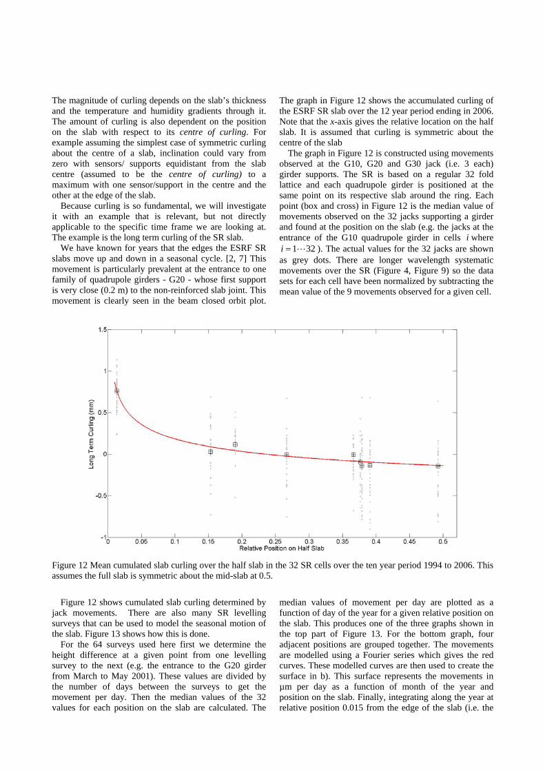
The graph in Figure 12 shows the accumulated curling of the ESRF SR slab over the 12 year period ending in 2006. Note that the x-axis gives the relative location on the half slab. It is assumed that curling is symmetric about the centre of the slab

The graph in Figure 12 is constructed using movements observed at the G10, G20 and G30 jack (i.e. 3 each) girder supports. The SR is based on a regular 32 fold lattice and each quadrupole girder is positioned at the same point on its respective slab around the ring. Each point (box and cross) in Figure 12 is the median value of movements observed on the 32 jacks supporting a girder and found at the position on the slab (e.g. the jacks at the entrance of the G10 quadrupole girder in cells i where

1 32= i ). The actual values for the 32 jacks are shown as grey dots. There are longer wavelength systematic movements over the SR (Figure 4, Figure 9) so the data sets for each cell have been normalized by subtracting the mean value of the 9 movements observed for a given cell.

Figure 12 Mean cumulated slab curling over the half slab in the 32 SR cells over the ten year period 1994 to 2006. This assumes the full slab is symmetric about the mid-slab at 0.5.

Figure 12 shows cumulated slab curling determined by jack movements. There are also many SR levelling surveys that can be used to model the seasonal motion of the slab. Figure 13 shows how this is done.

For the 64 surveys used here first we determine the height difference at a given point from one levelling survey to the next (e.g. the entrance to the G20 girder from March to May 2001). These values are divided by the number of days between the surveys to get the movement per day. Then the median values of the 32 values for each position on the slab are calculated. The

median values of movement per day are plotted as a function of day of the year for a given relative position on the slab. This produces one of the three graphs shown in the top part of Figure 13. For the bottom graph, four adjacent positions are grouped together. The movements are modelled using a Fourier series which gives the red curves. These modelled curves are then used to create the surface in b). This surface represents the movements in µm per day as a function of month of the year and position on the slab. Finally, integrating along the year at relative position 0.015 from the edge of the slab (i.e. the

position of the entrance to the G20 girder) produces the net movement as a function of month of the year c).

It is interesting to note in this graph a net upward motion of approximately 80 µm over the year. Referring back to Figure 12 we see there is a net upward movement of 1 mm (i.e. +0.77-(-0.14) µm over the 12 year period 1994 to 2006). The model which predicts 12×80 µm/year or 960 µm agrees remarkably well with the measured value of Figure 12.

There is no explanation for this net accumulated upward movement at the slab edge. However, it is tempting to suspect long term deformation due to the gradual drying (i.e. humidity change) of the slab.

Although cumulated movements due to slab curling at the SR joints are large, the inferred effect on the source is extremely small over the periods of time we are interested in. Using the surface in Figure 13 b) and subtracting movements of the slab between the position of the exit of the G30 girder (0.15) and the entrance of the G10 girder (0.38) we can calculate rotational movements due to slab curling over 30 minutes ranging between -0.22 nrad in the summer, and 0.46 nrad in the winter,. These modelled rotations are extremely small. However, as we shall see later, measured diurnal variations in SR temperature will induce larger movements.

Figure 13 The top three graphs a) show normalised median values for 64 levelling surveys at different relative positions on the slab (i.e. points at or clustered around 0.015, 0.15 and 0.37 from the edge where 0.5 is mid slab). Each of the points in these graphs is equivalent to one point (box and cross) in Figure 12. Graph b) shows modelled (idealised) movement of the slab as a function of relative position on the slab and month of the year. Graph c) shows the integrated motion – or net movement at relative position 0.015 near the edge of the slab, as a function of month of the year.

Source rotation movements In the previous section we discussed the effect of SR

slab curling over the long term. To study short term rotational movements, two HLS installations are used – one installed on the floor and the other on the SR machine. At this point it is important to distinguish

movements of the source (electron beam) and photon beam from what is measured with the HLS. The HLS measures movements of the slab on either side of the long straight section (LSS) in which the insertion devices are installed. They also measure movements of the quadrupole girders on either side of the insertion device that steer the electron beam. The actual movement of the

beam in the accelerator is more complex than this. Indeed past efforts to correlate realignment movements with those observed on the beamlines have never been straightforward. Nevertheless, one can expect that there is some correlation between ground and girder support movements and movements of the photon beam. Figure 14 shows the disposition of the HLS sensors used in this study.

Figure 14 HLS installations on the slab at either end of the LSS and on the machine G10 and G30 quadrupole girders on either end of the insertion device.

Inclination values for the SR slab are determined by differencing the readings on either side of the LSS and dividing by the distance between them. For the machine, a value is determined at the exit of the G10 and entrance of the G30 girders using a plane derived from the three HLS located on the girders.

1 2

1 2

10 30

1 2

−

−

−=

−=

hls hlsslab

hls hls

G Gmach

hls hls

R RRot

DR R

RotD

10GR is the value computed from the three HLS on the G10 girder downstream of the LSS, 30GR is the value computed from the three HLS on the G30 girder upstream of the LSS, and 1 2−hls hlsD is the distance between the exit of the G30 and entrance of the G10 girders.

Figure 15 shows expected rotational movements of the source and photon beam over periods ranging from 5 minutes (1 hour for the HLS on the machine) up to 8 weeks. First, the movements on the slab are smaller than on the machine. Nevertheless, they are still much larger than predicted from the model discussed in Figure 13 (i.e. < 1 nrad). There are two reasons for this. The first is the inherent uncertainty in predicting movements over 30 minutes from data measured once every month or two. The second is in the uncertainty of the HLS measurements. The flattening out of results below two hours is certainly due to the limitations of the HLS.

Figure 15 Inclination movements registered SR machine LSS. Rotational movement uncertainty on the floor is estimated to be 10 nrad and on the machine 50 nrad after 30 minutes.

There appears to be amplification between the movement measured on the floor and on the machine. This may be due to temperature. An angular movement of 100 nrad represents a change in height over the 6.5 m LSS of 0.65 µm. For example a temperature change (or uncertainty) in the order of 0.03˚C††

Finally, a dependence of rotational motion, and in principle correlated movements of the source, on diurnal temperature variation in the tunnel is observed. (

over 30 minutes would cause movements of this magnitude.

Figure 16) We shall return to this phenomenon later, but it is important to remark that there are movements in the order of ±50 nrad for temperature variations less than ±0.01 ˚C.

In conclusion, we can state that the 30 minute 100 nrad tolerance for the source is easily achieved.

Figure 16 There is a dependence of rotation across the LSS on diurnal temperature variation in the SR tunnel.

Rotational movements of the existing ESRF experimental hall slabs

An important parameter used to characterise soil behaviour is the Young’s modulus. It can be experimentally determined from the slope of a stress-strain curve created during tensile tests conducted on a sample of the material.‡‡

†† The beam is at 1.5 m. If we assume a combined thermal expansion coefficient of 15 µm/m/˚C, we can deduce a temperature change of approximately 0.03 ˚C for a movement of 0.65 µm.

The Young’s modulus of the

‡‡Young's modulus, also known as the tensile modulus, is a measure of the stiffness of an isotropic elastic material. It is defined as the ratio of

ESRF soil was estimated using a system of 29 HLS sensors installed on the experimental hall slab loaded with a 5 T mass. The experimental setup is shown in Figure 17. These results of this experiment are discussed in [8].

This system was also used to study the behaviour of the experimental hall slabs over the long term. It was the uniaxial stress over the uniaxial strain in the range of stress not exceeding the elastic limit. (http://en.wikipedia.org)

observed that the slabs were curling as a function of the temperature change in the experimental hall. To be more precise, slabs curl as a function of the change in the temperature (and/or humidity) gradient through them. Considering the temperature under the slab is essentially stable over several days, the main parameter driving the curling is the diurnal temperature variation in the experimental hall.

Figure 17 The setup of the HLS used to measure the Young’s modulus of the soil under the ESRF experimental hall slab and its long term behaviour. The top left photo shows the 5 T charge on the slab. The bottom drawing shows the disposition of the HLS on the slabs. There are nominally two slabs (blue and yellow in the figure). However, these slabs have a surface cut that effectively separates them into two parts. Each part behaves independently.

Figure 18 shows a characteristic example of the

cumulated curling of the slab centred on sensor 15 (HLS15 in Figure 17) after 4½ days starting 1 January 2010. There are maximal upward movements in the corner of the slab of nearly 110 µm and accompanying rotational movements along the direction of the photon beam of between -50 µrad and 100 µrad. What is remarkable is that these curling movements are induced by a temperature gradient change of -1.14 ˚C/18 cm.

Figure 20 shows the very clear dependence of slab curling on temperature gradient fluctuations that are driven by diurnal temperature variations in the experimental hall. Phase shifting the movements back 2 hours permits the development of a model indicating there is a 50 µm movement of the edge of the slab with respect to its centre for a change in temperature gradient through the slab of 1 ˚C.

Figure 18 Slab curling after 4½ days. There are maximum movements of nearly 110 µm in the slab corners with respect to its centre. The top graph shows the curling of the slab along the line HLS7 to HLS21 (see Figure 17 and the red lines on the surface and contour plots on the right hand side of this figure). The middle graph shows the rotational movements ranging between roughly -50 and +100 µrad. The bottom graph shows the temperature under the slab (blue) and the temperature on the slab surface (green) over the 4½ day period. The surface temperature decreases 1.22˚C and the ground temperature decreases 0.08˚C. Therefore a -1.14˚C/18 cm gradient change induces nearly 110 µm of curling.

Finally using the sampling techniques developed above

we can estimate the effect of slab curling ( )U rot as a function of time and position on the slab (refer to Figure 19). We can conclude from the rotational uncertainty after 30 minutes of between 180 nrad and 20 µrad that the 100 nrad tolerance is not respected on the existing experimental hall floor. This uncertainty is due to temperature fluctuations of much less than 0.1 ˚C. The temperature gradient uncertainty ( )U dT corresponding to this graph is shown in Figure 25.

There are two main points to note in these graphs. First is the clear diurnal effect of temperature; and second is the non-symmetric behaviour of slab curling. It is exemplified in the top two graphs of Figure 18. This characteristic behaviour may be due to the non-symmetric shape of the slab itself - refer to the slab centred of HLS15 in Figure 17.

Figure 19 Effect of slab curling U(rot) as a function of time and position on the slab. The blue and cyan crosses show the rotation at ±3.5 m from the centre of the slab, the green circles at ±2 m and the red and magenta squares near the edge of the slab at ±1 m from its centre. Estimated rotational movements at 30 minutes are range between 180 nrad near the slab centre to between 730 nrad to 2000 nrad on the slab edges.

Figure 20 In the top graph a) shows the movement of the six HLS sensors with respect to HLS15 along the alignment of HLS7 to HLS21 (i.e. along the alignment of the 0 mrad line of the photon beam – see also Figure 17) over the period 01-01-2010 to 31-05-2010. Graph b) shows temperature gradient through the slab over the same period. Graph c) shows the movement of HLS21 with respect to HLS15 (green) and the change in temperature gradient (blue) over the last week of the study. Phase shifting the movement in c) back 2 hours produces the correlation shown in d).

ADDITIONAL TEST CONFIGURATIONS Rotational movements of a reinforced piled slab

Two installations discussed in the section on translation movements on the long beam lines have three sensors installed on the experimental slab. These sensors can be used to study (infer) slab rotational movements by using the three measured heights with their known planimetric coordinates to determine a plane. The normal vector of this plane defines its tilts in two orthogonal directions. Choosing the coordinate system to be aligned along the photon beam, gives inclinations in the direction along and orthogonal to the beam. We are actually interested in the change in inclination with time so we calculate the plane for all of the readings and normalize by subtracting the first one.

Both slabs are 40 cm thick. However one of the two is built on a 2.64 m square lattice of 6 m deep piles. Piles were used in this case as reinforcement because the

ground at this site was considered particularly unstable. Results are for these two slabs are given in Figure 22

Both respect the 100 nrad tolerance up to 6 hours. Nevertheless, bearing in mind non-linear slab curling and the disposition of the HLS on these two slabs (see Figure 21) we must be careful in the interpretation of the results. It is unlikely that these slabs behave as rigid unbending ‘rocking’ blocks. They probably bend similarly to the SR slab shown in Figure 12. If this is the case, the majority of the movement will be at the edges of the slab and the rotational movement in the central part of the slab will be reduced.

One can conclude from Figure 10 and Figure 11 that the piled reinforcement is a success. Vertical movements are virtually the same as the slab built on an a priori stable site. It is noteworthy in Figure 22 however that rotational uncertainty as a function of time for the piled slab is the same as the non-piled slab. The main conclusion one can imply from this is that piles do not appear to change (i.e. reduce or increase) the effect of slab curling.

Figure 21 Disposition of the HLS sensors on the two independent experimental slabs. Both are 0.4 m reinforced slabs however due to ground instability, one slab is supported by a regular lattice of 6 m deep piles.

Figure 22 Rotational (rocking) motion of two experimental slabs located at the end of existing long beam lines.

Rotational movements of a beamline mirror mounted on a hexapod

Rotational instability of a mirror was considered to be the main cause of degraded experimental performance on one ESRF beamline. The mirror support was installed very close to a slab joint and so slab curling was a suspected cause for the degraded performance. An HLS was installed on the floor in the vicinity of the mirror hexapod support and on the mirror support itself. The installation is shown in Figure 23. The HLS was able to show that the slab was indeed curling and causing the hexapod support and mirror to tilt both along and across the direction of the photon beam. Induced tilts in the most sensitive direction along the beam were particularly important reaching up to 30 µrad on occasion. These rotational movements were very clearly correlated with

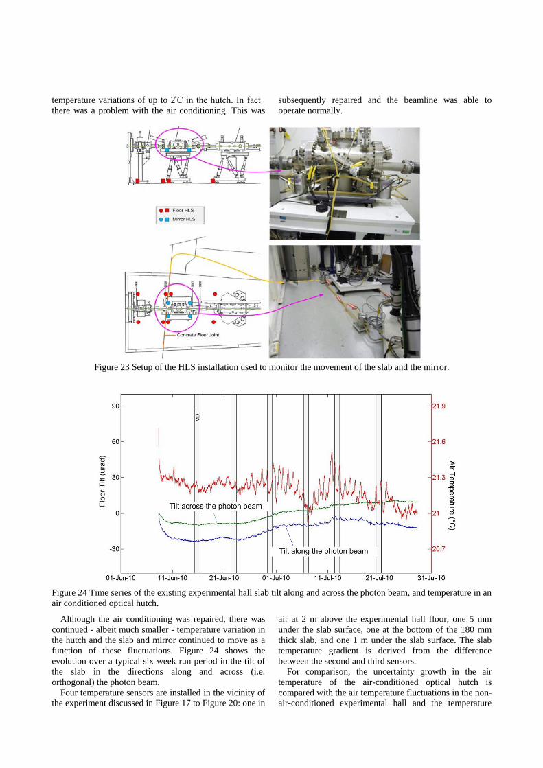
temperature variations of up to 2 ̊C in the hutch. In fact there was a problem with the air conditioning. This was

subsequently repaired and the beamline was able to operate normally.

Figure 23 Setup of the HLS installation used to monitor the movement of the slab and the mirror.

Figure 24 Time series of the existing experimental hall slab tilt along and across the photon beam, and temperature in an air conditioned optical hutch.

Although the air conditioning was repaired, there was continued - albeit much smaller - temperature variation in the hutch and the slab and mirror continued to move as a function of these fluctuations. Figure 24 shows the evolution over a typical six week run period in the tilt of the slab in the directions along and across (i.e. orthogonal) the photon beam.

Four temperature sensors are installed in the vicinity of the experiment discussed in Figure 17 to Figure 20: one in

air at 2 m above the experimental hall floor, one 5 mm under the slab surface, one at the bottom of the 180 mm thick slab, and one 1 m under the slab surface. The slab temperature gradient is derived from the difference between the second and third sensors.

For comparison, the uncertainty growth in the air temperature of the air-conditioned optical hutch is compared with the air temperature fluctuations in the non-air-conditioned experimental hall and the temperature

gradient fluctuations in the slab (Figure 25). The temperature gradient fluctuations in the experimental hall slab are derived from the time series shown in Figure 20.

Figure 25 Uncertainty growth in the optical hutch temperature (times series in Figure 24) the experimental hall air temperature and the temperature gradient through the slab.

The temperature under the slab evolves very slowly and has virtually no diurnal component in it. Considering this, from Figure 25 one can see that that the temperature at the slab surface is slightly attenuated with respect to the air temperature. Nevertheless, at 30 minutes there is an order of magnitude difference between the uncertainty in the air-conditioned optical hutch (i.e. 0.003 °C) and the slab temperature gradient (i.e. 0.03 °C) in the non air-conditioned experimental hall slab. Figure 26 shows the evolution in the slab tilt along and across the photon beam in the optical hutch. The results are at the 100 nrad tolerance limits and roughly a factor of 100 better than in the non- air-conditioned case shown in Figure 19 This demonstrates that air-conditioning is extremely effective in diminishing the effects of slab curling.

Figure 26 Uncertainty growth of the existing slab tilt along and across the photon beam in an air conditioned optical hutch (time series shown in Figure 24).

DISCUSSION AND SUMMARY

For the ESRF Upgrade program new beamlines, there are two tolerances that must be respected; vertical translations must be less than 15 µm, and combined rotational movements of the source and focusing

optics/sample ensemble must remain below 100 nrad, over 30 minutes.

Stability of 15 µm over 30 minutes is achieved on the existing ESRF installation and there is every reason to believe that it can be acheived on the new EX2 slab. However, beamlines are built to work for more than 30 minutes and long term site movements can be quite large – particularly in areas close to the rivers and the drainage system used to maintain the institute above the natural ground water level. Care must be taken to anticipate long term subsidence and/or uplift and so that sufficient stroke is designed into alignment systems. Finally, although 15 µm over 30 minutes appears to be easily achievable, applying the model in Figure 11 indicates that the tolerance will be exceeded in less than 3 days on a 250 m long beamline and after one week, the vertical uncertainty is more than three times the acceptable tolerance for a 250 m long beamline. These numbers indicate that long beamlines must be realigned regularly.

If translational stability is achievable, rotational stability is far more challenging. Although we can reasonably expect the rotational tolerance of the source to be respected, the required 100 nrad over 30 minutes is exceeded by a factor of three in the non-air-conditioned case at even 1 m from the centre of the existing ESRF slab. This is due to slab curling.

Considering the deep ground temperature is virtually stable over several days, the main driving force in slab curling is the temperature variation at the surface of the slab. Even very small variations can induce relatively large movements. Theoretically, this effect is exacerbated in thicker slabs. Air conditioning reduces the effect dramatically. The second main consideration in slab curling is the proximity to the slab edge. Supports near the edge of a slab experience much larger rotation than those nearer the centre of the slab (curling). The following three general points can help to reduce the effects of slab curling: • sensitive equipment (supports) should be installed far

from the edge of the slab; • install supports symmetrically about the centre of

curling; and especially, • reduce slab surface temperature variations to a

minimum.

ACKNOWLEDGMENTS I would like to extend special thanks to all of the members of the ESRF ALGE group, but in particular to G. Gatta, B. Perret and to L. Maleval for their meticulous attention to the different HLS installations at the ESRF. I would also like to thank Y. Dabin and L. Zhang of the ESRF ISDD Advanced Analysis and Modelling group, and E. Bruas and P. MacKrill of the EX2 Project Management team for their fruitful discussions on the existing as well as the planned EX2 slabs, and to L. Farvacque of the ESRF Accelerator and Source Division for discussing how the beam should behave

when the ground moves. Finally I would like to thank the ESRF staff and scientists for permitting the long, sometimes arduous measurements to be made on or near their beamlines and in particular: R. Ruffer, P. Glatzel,

P. Cloetens, G.Vaughan, M. Burghammer, A. Bravin, and J. Baruchel.

REFERENCES [1] ESRF ed., The European Synchrotron Radiation

Facility Science and Technology Programme 2008 to 2017 (http://www.esrf.eu/AboutUs/Upgrade/documentation/purple-book/, 2007).

[2] Martin, D., et al. Long Term Site Movements at the ESRF. in Ninth International Workshop on Accelerator Alignment. 2006. Stanford Linear Accelerator Center, Stanford University, California.

[3] Martin, D., Vertical Ground Movement Signatures Observed on the ESRF Site, in ESRF Experiments Division Tuesday event. March 10, 2009 ESRF.

[4] Menard, G., Mesure de l’affaissement actuel de la cuvette grenobloise par comparaisons de nivellements. 2008: Pôle Grenoblois Risques Naturels - Conseil Général d'Isère.

[5] Martin, D. Some Reflections on the Validation and Analysis of HLS Data. in Eighth International Workshop on Accelerator Alignment. 2004. CERN, Geneva Switzerland.

[6] Efron, B. and R.J. Tibshirani, An introduction to the bootstrap. Monographs on statistics and applied probability. 1993, New York ; London: Chapman & Hall.

[7] Martin, D. Deformation Movements Observed at the European Synchrotron Radiation Facility. in The 22nd Advanced ICFA Beam Dynamics Workshop on Ground Motion in Future Accelerators. 2000. Stanford Linear Accelerator Center, Stanford University (USA).

[8] Zhang, L., et al. Preliminary study for the slab of the ESRF experiment hall extension. in MEDSI. 2010. Oxford, U.K.