SOME GENERICITY ANALYSES IN NONPARAMETRICSTATISTICS‡

MAXWELL B. STINCHCOMBE

Abstract. Many nonparametric estimators and tests are naturally set in in-finite dimensional contexts. Prevalence is the infinite dimensional analogue offull Lebesgue measure, shyness the analogue of being a Lebesgue null set.A prevalent set of prior distributions lead to wildly inconsistent Bayesian

updating when independent and identically distributed observations happen inclass of infinite spaces that includes Rn and N.For any rate of convergence, no matter how slow, only a shy set of tar-

get functions can be approximated by consistent nonparametric regressionschemes in a class that includes series approximations, kernels and other locallyweighted regressions, splines, and artificial neural networks.When the instruments allow for the existence of an instrumental regression,

the regression function only exists for a shy set of dependent variables. Theinstruments allow for existence in a counterintuitive dense set of cases, shynessis an open question.A prevalent set of integrated conditional moment (ICM) specification tests

are consistent, a dense subset of the finitely parametrized ICM tests are con-sistent, prevalence is an open question.

Date: December 10, 2002.‡Many thanks Xiaohong Chen, Stephen Donald, and Haskell Rosenthal, Dan Slesnick, HalWhite, and Paul Wilson for helpful conversations about this paper. Tom Wiseman and Jeff Elyhelped with some difficult terminological issues, but I’m not sure they want to be thanked.

1

1. Introduction

For some, but not all prior distributions, Bayesian updating based on i.i.d. real-

valued random variables is consistent. Given a sequence rn → 0, for some, but notall functional relations f(x) = E(Y |X = x), consistent nonparametric regressiontechniques for estimating f converge at rate O(rn). Under the compact operatorassumptions used in devising estimators for instrumental regressions, for some,

but not all dependent variables, instrumental regressions exist. Some, but not

all, integrated conditional moment (ICM) tests are consistent for any deviation

from the null.

These observations mean that absolute answers to a number of important ques-

tions are not possible. We cannot say that Bayesian updating is consistent. We

cannot say that all functions are O(rn) approximable. We cannot say that instru-mental regressions always exist. We cannot say that all ICM tests are consistent.

This paper answers the questions that flow from the lack of absolute answers.

“How big is the set of priors for which Bayesian updating is consistent?” “How

big is the set of functions approximable at rate O(rn)?” “How big is the set ofdependent variables for which instrumental regressions exist?” Finally, “How big

is the set of consistent ICM tests?”

The answers to these questions are given in terms of prevalence and shyness.

The nonparametric estimators and tests considered here are naturally set in infi-

nite dimensional contexts. Prevalence is the infinite dimensional analogue of full

Lebesgue measure, or genericity, shyness the analogue of being a Lebesgue null

set, of being non-generic.

In short, the answers are:

1. Given a true distribution θ with infinite support in a locally compact space,

it is a prevalent property of priors that with probability 1, for every strictly

positive ε and every non-empty open G, the Bayesian posterior distribution

assign mass at least 1 − ε to G infinitely often. Thus, Bayesian updatingcan only be consistent for a shy set of prior distributions.

2. Given any rate rn → 0, only a shy set of functions is approximable at rateO(rn) using any of a wide class of nonparametric estimation techniques.This means that the regularity conditions invoked to guarantee faster rates

of estimator convergence, usually smoothness assumptions, restrict attention

2

to a shy class of functions, something that is at odds with the intended

interpretations of consistency results.

3. Given the compact operator assumptions invoked to devise estimation tech-

niques, instrumental regressions exist only for a shy set of dependent random

variables. The sufficient conditions for the compact operator assumptions

are themselves only satisfied for a shy set of distributions of the explanatory

and instrumental variables.

4. Finally, within the set of ICM tests, consistency is prevalent. Within the set

of ICM tests that are finitely parametrized, consistency is dense, whether or

not it is prevalent is an open question.

Genericity analyses run the risk of being wrong-headed. For example, suppose

an estimation technique is consistent and/or efficient only if the mean, µ, and

the standard deviation, σ, of the population are equal. When µ and σ are viewed

as unrelated (beyond both being positive), the whole positive orthant must be

considered. Relative to the positive orthant, the diagonal along which µ = σ is

a non-generic set. In this case, the technique would be judged to be generically

inconsistent and/or inefficient. This conclusion is not informative if (µ, σ) is

known to lie on the diagonal (as it might in some counting processes or after

some variance stabilizing transformations). More generally, the conclusion that

a set E ⊂ X is “large” relative to X can happen because X is “too small,” theconclusion that a set E ⊂ X is “small” relative to X can happen because X is “toolarge.” Each of sections concludes with an examination of these interpretational

issues, and the final section considers these issues in a unified fashion.

The next section contains the necessary background on genericity for the in-

finite dimensional contexts considered here. The subsequent sections discuss,

in turn, the generic inconsistency of Bayesian updating, the shyness of the set

of regression functions that can be approximated at any given rate, the generic

properties of nonparametric instrumental variable regressions, and the generic

consistency of integrated conditional moment tests. The material in the section

on nonparametric instrumental variable regression depends slightly on the ma-

terial in the section on general nonparametric regression. Aside from this, the

sections are mutually independent. Proofs are gathered in the appendix.

3

2. Small Sets and Large Sets

Throughout, X denotes an infinite dimensional, locally convex, topological vec-

tor space that is also a complete separable metric (csm) space. From Rudin (1973,

Theorem 1.24, p. 18), the topology on X can be metrized by a translation invari-

ant metric d(·, ·), that is, d(x, y) = d(x + z, y + z) for all x, y, z ∈ X. This classof spaces includes (but is not limited to):

1. separable Banach spaces such as the Lp(Ω,F , P ) spaces, 1 ≤ p < ∞, Fcountably generated;

2. C(X), the continuous functions with the sup norm when X is compact;

3. C(X) with the topology of uniform convergence on compact sets when X is

locally compact and separable;

4. the Sobolev spaces Spm(Rr, µ) defined as the metric completion of Cpm(R

r, µ),

the space of m times continuously differentiable functions, m ≥ 0, on Rrhaving finite norm ‖f‖p,m,µ =

∑|α|≤m

[∫ |Dαf(x)|p dµ(x)] 1p , p ∈ [1,∞), µ aBorel probability measure on Rr;

5. Cm(X), the space of m times continuously differentiable functions on a

compact X with the norm∑|α|≤nmaxx∈X |Dαf(x)| .

There are two notions of rarity available for X. The topological notion called

meagerness is due to Baire (1899, §59-61, pp. 65-67). The measure theoreticnotion called Haar zero sets is due to Christensen (1974, Ch. 7). Its properties

and applications were more thoroughly investigated under the name of shy sets

by Hunt, Sauer and Yorke (HSY, 1992), who especially applied these techniques

to the study of the generic behavior of dynamical systems. There are subtle and

difficult problems in extending shyness to a definition of non-generic for subsets of

convex subsets of vector spaces that are themselves shy, e.g. spaces of probability

measures. These problems were discovered and resolved by Anderson and Zame

(2001).

2.a. Meager and residual sets. A closed set with no interior seems small.

Definition 2.1. A set S is nowhere dense if its closure has no interior. A set

S is meager if it can be expressed as a countable union of nowhere dense sets.

A set E is residual or Baire large if it is the complement of a meager set.

4

Baire large sets are, equivalently, the countable intersection of open dense sets.

The countable union of meager sets is meager, the countable intersection of Baire

large sets is a Baire large set. Because X is a csm space, any Baire large subset is

dense, and to some extent this justifies thinking of residual sets as being “large”

or “generic”. Baire large sets can have Lebesgue measure 0 and seem quite small

in Rk (k <∞ throughout).Example 2.1. Let qn be an enumeration of the vectors in R

k with rational coor-

dinates. For any rational ε > 0, let Eε be the union of open balls centered at qn,

∪nB(qn, ε/2n). Eε is an open dense subset of Rk having Lebesgue measure lessthan ε. The set E = ∩εEε is a residual set having Lebesgue measure 0.2.b. Shy and prevalent sets. For Rk, we have the following.

Lemma 2.1. For a universally measurable S ⊂ Rk, the following are equivalent1. Λk(S) = 0 where Λk is k-dimensional Lebesgue measure,

2. Gk(S) = 0 where Gk is a non-degenerate Gaussian distribution, and

3. there exists a compactly supported probability η such that η(S + x) = 0 for

all x ∈ Rk.The third condition in Lemma 2.1 generalizes to X. Taking the measure η to

be the continuous linear image of Uk, the uniform distribution on [0, 1]k, is so

useful that it merits a special name.

Definition 2.2 (Christensen. Hunt, Sauer, and Yorke). A subset S of a univer-

sally measurable S ′ ⊂ X is shy if there exists a compactly supported probabilityη such that η(S ′ + x) = 0 for all x. S is finitely shy if η can be taken the

continuous linear image of Uk for some k. The complement of a (finitely) shy set

is a (finitely) prevalent set.

From HSY (1992, Facts 2′ and 3′′), no S containing an open set can be finitelyshy in X so that prevalent sets are dense, and countable unions of shy sets are

shy, equivalently, countable intersections of prevalent sets are prevalent

2.c. Approximately flat sets. For A,B ⊂ X, define A + B = a + b : a ∈A, b ∈ B. For any sequence of An of sets, [An i.o.], read as “An infinitelyoften,” is defined as

⋂m

⋃n≥mAn. In a similar fashion, [An a.a.], read as “An

5

almost always,” is defined as⋃m

⋂n≥mAn. The following definition and Lemma

will be used frequently.

Definition 2.3. A set F ⊂ X is approximately flat, if for every ε > 0, thereis a finite dimensional subspace W of X such that F ⊂W +B(0, ε) where B(x, r)

is the ball around x with radius r.

Any finite union of approximately flat sets is approximately flat, and every

compact set is approximately flat — let W be the span of a finite ε-net. The

following is the basic lemma used Stinchcombe (2001).

Lemma 2.2. For any sequence, Fn, of approximately flat sets and any rn → 0,the set [(Fn +B(0, rn)) i.o.] is shy.

Taking Fn ≡ F shows that the closure of any approximately flat (e.g. any

compact set) set is shy.

One intuition for the shyness of [(Fn + B(0, rn)) i.o.] comes from how small

approximately flat sets are. If W d is a d-dimensional subspace of Rk, then, as a

proportion of the unit ball, W d + B(0, ε) is on the order of εk−d. This leads oneto suspect that approximately flat sets are “small” in infinite dimensional X’s.

2.d. Shy subsets of convex sets. Suppose that C is a convex subset of Rk.

Defining S ′ ⊂ C to be shy relative to C by asking that S ′ = S ∩ C for some shyS ⊂ Rk make C a shy subset of itself if dim (C) < k. However, taking aff (C)

to be the smallest affine subspace containing C and using the lower dimensional

Lebesgue measure on aff (C) delivers the appropriate definition.

An example directly relevant to this paper demonstrates that the affine sub-

space approach does not generally work in X. Take X to be the set of countably

additive, finite, signed measures on 2N, C = ∆(N) ⊂ X to be the probabilitymeasures on 2N. ∆(N) is a finitely shy subset of X. (Let η be the uniform dis-

tribution on the line L joining the 0 measure and any point mass, δn. For any

x ∈ X, L ∩ (∆(N) + x) contains at most one point, so that η(∆(N) + x) = 0.)However, aff (∆(N)) = X.

Working from the “outside,” that is, with aff (C), is not appropriate in X.

The path-breaking work of Anderson and Zame (2001) give a definition of shy

subsets of C that works from the “inside.” For any c ∈ C, C convex, and anyε > 0, the set εC + (1 − ε)c is a convex subset of C that shrinks C toward c.

6

For a universally measurable C ⊂ X, ∆K(C) denotes the compactly supportedprobability measures on C.

Definition 2.4 (Anderson and Zame). Let C be a convex subset of X that is

topologically complete in the relative topology. A subset S of a universally mea-

surable S ′ ⊂ C is shy relative to C if for all c ∈ C, all neighborhoods Uc of c,and all ε > 0, there exists a η ∈ ∆K(C) such that η(Uc ∩ [εC + (1 − ε)c]) = 1and (∀x ∈ X)[η(S ′ + x) = 0]. S is finitely shy relative to C if there existsa if η ∈ ∆K(C) that is the continuous affine image of Uk for some k such that(∀x ∈ X)[η(S ′ + x) = 0]. The complement of a (finitely) shy set is a (finitely)prevalent set.

Anderson and Zame (2001) show that finite shyness is sufficient for shyness,

that the countable union of shy sets is shy, and that shyness is equivalent to the

“Lebesgue measure on aff (C)” definition in Rk. They demonstrate the utility

of their definition of shyness relative to convex sets in a number of contexts in

theoretical economics.

For S ⊂ C, C a convex subset of X, coS is the closure of its convex hull. For

S, T ⊂ C, rel intS(T ) is the interior of S relative to T . The following sufficient

condition for shyness relative to a convex set will be useful below.

Lemma 2.3. Let C be a convex subset of X that is topologically complete in the

relative topology. If coS has empty interior relative to C, then S is a finitely shy

subset of C.

2.e. Interpretational issues. In Rk, Lemma 2.1 ties together Lebesgue mea-

sure, a probabilistic interpretation, and a translation invariant property of the

smallness of a set S. Lebesgue measure fails to extend to X because there is no

translation invariant measure on X assigning positive mass to any open set. If

there were, it would have to assign equal, and strictly positive mass to every open

ball B(x, ε/4). Since X is infinite dimensional, every B(y, ε) contains countably

many disjoint balls with radius ε/4, and the measure assigned to every open set

would therefore be infinite.

Probability measures on csm spaces are tight, that is, for every ε > 0, there

is a compact set, Fε, with P (Fε) > 1 − ε. Probabilistic interpretations fail to

extend to X directly because the tightness of any probability P on X implies

7

that P (S) = 1 for S being the countable union of compact, hence shy, sets.

Probabilistic interpretations of shyness also fail to be approximately true.

Let Yi be an independent and identically distributed (iid) sequence of random

variables distributed P . Suppose that that rn → 0, and that Nn → ∞. Apoint x ∈ X is (rn, Nn)-lonely if P∞(A(x)) = 0 where A(x) = [An(x) i.o.],An(x) = d(Yi, x) < rn for some i ≤ Nn. In other words, the x is lonely if,with probability 1, B(x, rn) eventually receives no more visits from Y1, . . . , YNn.

Stinchcombe (2001) shows that, no matter how slowly rn goes to 0 or how quickly

Nn goes to ∞, a prevalent set of points are (rn, Nn)-lonely.

3. The Generic Inconsistency of Bayesian Updating

Bayesian updating approaches to and understandings of statistical problems

and results are widespread. It is therefore striking that Bayesian updating is

generically inconsistent. The classic result is that for a Baire large set of pri-

ors on the distributions on the integers, Bayesian updating is wildly inconsistent

(Freedman 1965). Since Baire large sets can be shy, and several of the construc-

tions in Freedman’s proof use sets that turn out to be shy, one might have hoped

(as the author did) that this wild inconsistency was non-generic.

Bayesian updating and optimization in the face of uncertainty are intimately

tied, nowhere more so than in the theory of learning. Nachbar’s (1997) crucial

result for infinitely repeated games is that, when combined with optimization,

Bayesian updating of priors about other players’ repeated game strategies is

leads the players to play strategies that others were certain were not going to

be played. Generic inconsistency implies that for interesting single agent games,

Bayesian updating is “objectively” sub-optimal. It also provides a optimizing

rationalization of fads, bubbles, and other seemingly irrational behavior.

3.a. Overview for real-valued random variables. Suppose that we observe

a sequence of iid R-valued random variables (Yn)n∈N. Let θ ∈ ∆(R) denote thetrue, full support distribution of each Yn. Let θ

∞ denote the distribution of thesequence of Yn’s. A prior distribution, µ, is a distribution on ∆(R). Notationally,

µ ∈M = ∆(∆(R)).After observing a partial history ht = (x1, . . . , xt) ∈ Rt, the posterior beliefs

µ(·|ht) are formed using Bayes’ Law. Bayesian updating is consistent if for θ∞

8

almost all histories, posterior beliefs converge, in the weak∗ topology, to puttingmass 1 on θ, µ(·|ht)→w∗ δθ.Null sets can cause serious problems in updating — conditional probabilities

are arbitrary on null sets, and the set of observed ht typically belong to null sets.

The best solution is to use densities. To avoid these issues, one must work in a

countably infinite space such as N.

Fix a full support, σ-finite reference measure, λ, on R, e.g. Lebesgue measure.

Let Cλ+ denote the set of continuous, non-negative functions f such that∫Xf dλ =

1, Cλ++ ⊂ Cλ+ is the set of strictly positive f . Each f ∈ Cλ+ is uniquely associatedwith the probability θf ∈ ∆(X) defined by θf (A) =

∫Af dλ.

Updating after partial history ht = (x1, . . . , xt) ∈ X t is done using the valuesof the densities at ht and the prior, µ, MλB ,

µ(B|ht) :=∫BΠti=1f(xt) dµ(f)∫

Cλ+Πti=1f(xt) dµ(f)

, B ⊂ Cλ+.(1)

MλB ⊂Mλ are those beliefs which will never involve division by 0 in (1),MλB = µ ∈M : µ(Cλ+) = 1, ∀(x1, . . . , xt) µ(f : Πti=1f(xi) > 0) > 0 .(2)

Theorem 3.1 shows that for any full support θ, Bayesian updating is consistent

only for a shy set of µ ∈ MλB. This is true even when θ = θf for some f ∈ Cλ+.One step in the proof contains some insight into how inconsistency can arise.

Example 3.1. For arbitrary full support θ and θ, there is a dense set of priorswith the property that θ∞-a.e., posterior beliefs converge to θ.To see why, let M ⊂ M denote the set of beliefs, ν, that rule out some non-empty, open V ⊂ R, that is, for which V , ν(θ : θ(V ) > 0) = 0. Let D be theset of µ’s of the form α0δθ +

∑i≤I αiνi where α0 > 0 and νi ∈ M . D is easily

seen to be dense in MλB. Since the true θ is full support, every non-empty open V

will be visited infinitely often θ∞-a.e. Therefore, for every µ ∈ D, only the fullsupport θ can have positive posterior weight in the limit, that is, µ(·|ht)→w∗ δθ.It is important to note that the prior beliefs used in Example 3.1 are not an

indication of the kind of priors that one must have for Bayesian updating to be

inconsistent, they are but a device used in the proof. Indeed, a direct implication

of Theorem 3.1 is that Bayesian updating is only consistent for a shy subset of the

full support beliefs in ∆(Cλ++). By contrast, the priors in Example 3.1 may put

9

mass less than 1 on ∆(Cλ++). The inconsistency of Example 3.1 only scratches

the surface of how badly Bayesian updating of generic priors behaves.

A pair (µ, θ) is erratic written µ ∈ err(θ), if for all non-empty open subsetsG of ∆(R), lim supt µ(G|ht) = 1 for a set of histories having θ∞ probability 1.Theorem 3.1 shows that for any full support θ ∈ ∆(R), err(θ) is prevalent in MλB.Because the set of full support µ is a prevalent subset ofMλB, the result does not

arise from some kind of failure of support conditions. For the same reason, the

result continues to hold if one restricts attention to beliefs that are full support

on the set of probabilities having only strictly positive densities. Further, since

the result holds for any full support θ, it also does not arise by picking the true

θ to be outside the set supporting the prior beliefs.

3.b. Generic inconsistency. Fix an infinite, locally compact, complete, sepa-

rable metric (csm) space (X, d) with X denoting Borel sigma-field. (A space is lo-cally compact if every point has a neighborhood with compact closure. The spaces

R` and N are locally compact, infinite dimensional topological vector spaces are

not.) ∆(X) denotes the set of (countably additive, Borel) probabilities on X . Aniid sequence of draws, (Yn)n∈N, is made according to a distribution θ ∈ ∆(X),and θ∞ denotes the corresponding product distribution on XN. Prior beliefs, µ,are points in ∆(∆(X)), the set of distributions on the set of distributions on X.

Both ∆(X) and ∆(∆(X)) are csm’s in the weak∗ topology.Define θµ ∈ ∆(X) by θµ(E) =

∫Θθ(E) dµ(θ) for µ ∈ ∆(∆(X)). If θµ 6 θ, the

choice of version of the conditional probabilities matters quite sharply. As noted

above, to relate µ to the updated, versions of µ conditional on finite histories of

draws, one must make a whole system of coordinated choices of versions. This will

be done by assuming that the µ’s under study put mass 1 on the dense set of θ’s

having continuous densities with respect to some full support reference measure.

Throughout, a simple reference case has X countable and discrete, in which case

the σ-finite reference measure, λ, can be taken to be counting measure, and all

probabilities have densities with respect to λ.

1. λ is a full support, σ-finite reference measure on X . C(X) is the set ofcontinuous functions on X. Cλ+ ⊂ C(X) is the set of non-negative f such

that∫Xf dλ = 1, Cλ++ ⊂ Cλ+ is the set of strictly positive f . Each f ∈ Cλ+ is

10

associated with a probability θf ∈ ∆(X) defined by θf(A) =∫Af dλ. When

X is countable and discrete, Cλ+ = ∆(X).

2. Both Cλ++ and Cλ+ are Gδ’s in the csm ∆(X), implying that there are com-

plete separable metrics, d++ and d+ inducing the weak∗ topology. (A Gδ is

a countable intersection of open sets. The relative topology on any Gδ in

a csm can be metrized with a complete separable metric. It is easy to give

explicit metrics making Cλ+ and Cλ++ into csm’s. )

3. Mλ ⊂ ∆(∆(X)) denotes the set of probabilities on probabilities ∆(Cλ+),while Mλ++ denotes ∆(C

λ++). M

λB are those for which Bayes updating using

densities will never involve division by 0, formally,

MλB = µ ∈Mλ : ∀(x1, . . . , xt) µ(f : Πti=1f(xi) > 0) > 0 .From the definitions, Mλ++ ⊂ MλB ⊂ Mλ. It can be shown that Mλ++ is aconvex, topologically complete, prevalent subset of the convex csm Mλ, and MλBis a Gδ, hence topologically complete.

Assuming that µ ∈ MλB, updating after partial history ht = (x1, . . . , xt) ∈ X tis done using the values of the densities at ht and the prior, µ,

µ(B|ht) :=∫BΠti=1f(xt) dµ(f)∫

Cλ+Πti=1f(xt) dµ(f)

, B ⊂ Cλ+.(3)

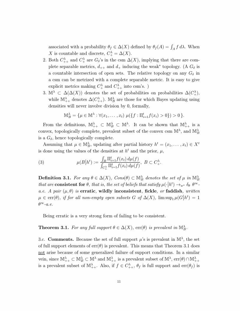
Definition 3.1. For any θ ∈ ∆(X), Cons(θ) ⊂ MλB denotes the set of µ in MλBthat are consistent for θ, that is, the set of beliefs that satisfy µ(·|ht)→w∗ δθ θ∞-a.e. A pair (µ, θ) is erratic, wildly inconsistent, fickle, or faddish, written

µ ∈ err(θ), if for all non-empty open subsets G of ∆(X), lim supt µ(G|ht) = 1θ∞-a.e.

Being erratic is a very strong form of failing to be consistent.

Theorem 3.1. For any full support θ ∈ ∆(X), err(θ) is prevalent in MλB.

3.c. Comments. Because the set of full support µ’s is prevalent in Mλ, the set

of full support elements of err(θ) is prevalent. This means that Theorem 3.1 does

not arise because of some generalized failure of support conditions. In a similar

vein, since Mλ++ ⊂MλB ⊂Mλ and Mλ++ is a prevalent subset of Mλ, err(θ)∩Mλ++is a prevalent subset of Mλ++. Also, if f ∈ Cλ++, θf is full support and err(θf ) is

11

prevalent. Theorem 3.1 does not arise because the full support θ is necessarily

outside the set of probabilities supporting µ.

The continuity of the densities can be weakened — the result holds if the set

of densities being considered are continuous with respect to a metric for which:

(a) λ is still full support, and (b) the Borel σ-field is still σ-field X .WhenX ⊂ R, the Glivenko-Cantelli theorem tells us that θ∞-a.e., the empiricalcdf converges uniformly to the cdf of θ. Generically, Bayes estimators behave

much differently, not converging to the true θ nor to anything else. When X = N,

Freedman (1965) shows that a Baire large set of (µ, θ) pairs in ∆(∆(N))×∆(N)are erratic. This uses a “Fubini” theorem for Baire sets. Anderson and Zame

(2001, Example 4, p. 57) show that no such Fubini result is available for prevalent

sets.

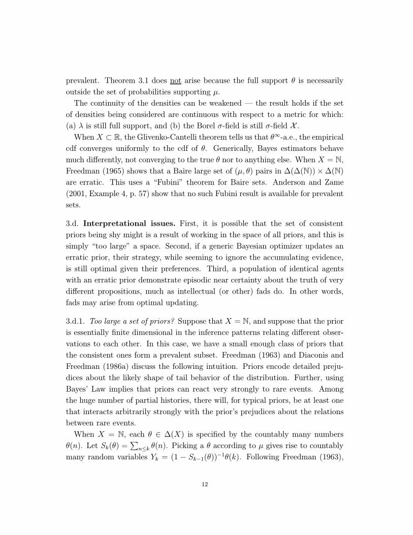
3.d. Interpretational issues. First, it is possible that the set of consistent

priors being shy might is a result of working in the space of all priors, and this is

simply “too large” a space. Second, if a generic Bayesian optimizer updates an

erratic prior, their strategy, while seeming to ignore the accumulating evidence,

is still optimal given their preferences. Third, a population of identical agents

with an erratic prior demonstrate episodic near certainty about the truth of very

different propositions, much as intellectual (or other) fads do. In other words,

fads may arise from optimal updating.

3.d.1. Too large a set of priors? Suppose that X = N, and suppose that the prior

is essentially finite dimensional in the inference patterns relating different obser-

vations to each other. In this case, we have a small enough class of priors that

the consistent ones form a prevalent subset. Freedman (1963) and Diaconis and

Freedman (1986a) discuss the following intuition. Priors encode detailed preju-

dices about the likely shape of tail behavior of the distribution. Further, using

Bayes’ Law implies that priors can react very strongly to rare events. Among

the huge number of partial histories, there will, for typical priors, be at least one

that interacts arbitrarily strongly with the prior’s prejudices about the relations

between rare events.

When X = N, each θ ∈ ∆(X) is specified by the countably many numbersθ(n). Let Sk(θ) =

∑n≤k θ(n). Picking a θ according to µ gives rise to countably

many random variables Yk = (1 − Sk−1(θ))−1θ(k). Following Freedman (1963),

12

a prior µ is tail-free if µ(Sk < 1) = 1 for all k, and there exists a K such

that the random vector (θk)Kk=1 and the random variables YK+1, YK+2, . . . are

mutually independent (see Ferguson (1973) for a wide set of applications of these

ideas). With tail-free priors, large observations in N have no information about

the smaller observations, and there is essentially only a finite dimensional set of

relations between the different observations.

The extent to which these intuitions generalize to more general X is somewhat

unclear, see Arnold et al (1984) and Diaconis and Freedman (1986b) for relatively

natural settings (competing risks and location estimators respectively) in which

Bayes estimators are not consistent.

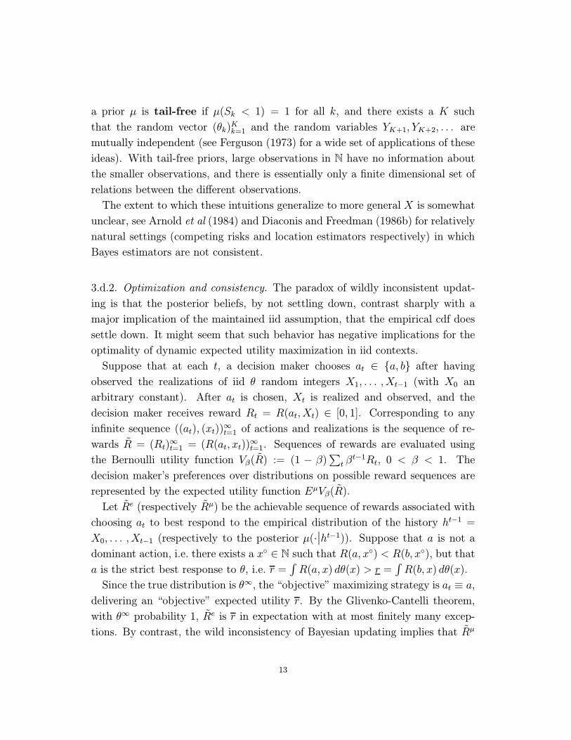
3.d.2. Optimization and consistency. The paradox of wildly inconsistent updat-

ing is that the posterior beliefs, by not settling down, contrast sharply with a

major implication of the maintained iid assumption, that the empirical cdf does

settle down. It might seem that such behavior has negative implications for the

optimality of dynamic expected utility maximization in iid contexts.

Suppose that at each t, a decision maker chooses at ∈ a, b after havingobserved the realizations of iid θ random integers X1, . . . , Xt−1 (with X0 anarbitrary constant). After at is chosen, Xt is realized and observed, and the

decision maker receives reward Rt = R(at, Xt) ∈ [0, 1]. Corresponding to anyinfinite sequence ((at), (xt))

∞t=1 of actions and realizations is the sequence of re-

wards R = (Rt)∞t=1 = (R(at, xt))

∞t=1. Sequences of rewards are evaluated using

the Bernoulli utility function Vβ(R) := (1 − β)∑t βt−1Rt, 0 < β < 1. The

decision maker’s preferences over distributions on possible reward sequences are

represented by the expected utility function EµVβ(R).

Let Re (respectively Rµ) be the achievable sequence of rewards associated with

choosing at to best respond to the empirical distribution of the history ht−1 =

X0, . . . , Xt−1 (respectively to the posterior µ(·|ht−1)). Suppose that a is not adominant action, i.e. there exists a x ∈ N such that R(a, x) < R(b, x), but thata is the strict best response to θ, i.e. r =

∫R(a, x) dθ(x) > r =

∫R(b, x) dθ(x).

Since the true distribution is θ∞, the “objective” maximizing strategy is at ≡ a,

delivering an “objective” expected utility r. By the Glivenko-Cantelli theorem,

with θ∞ probability 1, Re is r in expectation with at most finitely many excep-tions. By contrast, the wild inconsistency of Bayesian updating implies that Rµ

13

is r infinitely often. This seems to indicate that patient optimizers will prefer

Re to Rµ, that the consistency embodied in the empirical cdf approach leads to

higher payoffs, at least for patient decision makers.

Formalizing such an argument would require the inequality

EδθVβ(Re) > EδθVβ(R

µ),(4)

and it is here that the fallacy appears clearly. It is quite easy to give generic µ’s

and θ in the support of µ satisfying (4). However, an expected utility chooses

actions bearing in mind a wide range of possibilities, and knowing that this cau-

tion may involve the “wrong” action being chosen from time to time. Evaluating

a course of action under δθ, that is, under certainty about the true distribution

is, from the decision maker’s point of view, an entirely irrelevant exercise.

3.d.3. Fads. Suppose that the action set a, b above is replaced by an infiniteset with the property each action is the unique maximizer of R(a, θ) for some

θ ∈ ∆(N). Another way to understand the oddity of wild inconsistency is thatnew observations on the same process arrive, and beliefs and actions will wander

arbitrarily far away from the historical record infinitely often. If a large popula-

tion of identical agents behaves in so erratic a fashion, one is tempted to look for

a model of irrationality, perhaps a model of informational cascades, or a model

of bubbles, or to look for exogenous sources of variability, in short, to look for a

model of fads. One point to be taken from the present result is that there is a huge

variety of rational behavior, even in the quite limited case of iid observations.

4. Rates of Convergence for Nonparametric Regression

Suppose that interest centers on finding f(x) = E (Y |X = x), and the target

function f belongs to separable Banach space X, typically an L2(R`, µ) space or

a Sobolev space, Spm(R`, µ), of smooth functions. In this section, X is assumed

to be a Banach space. For any rate of approximation rn → 0, no matter howslow, only a shy set of functions f are O(rn)-approximable by a wide class ofthe available nonparametric regression techniques. The present analysis concerns

only the deterministic part of the regression error, not the part due to noise in

the observations.

Consistency results for nonparametric regression techniques show that the ap-

proximation error converges to 0. Rate of convergence results show that the

14

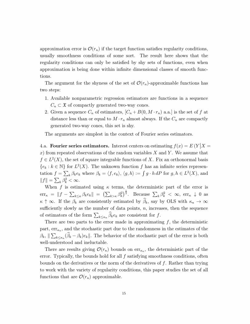
approximation error is O(rn) if the target function satisfies regularity conditions,usually smoothness conditions of some sort. The result here shows that the

regularity conditions can only be satisfied by shy sets of functions, even when

approximation is being done within infinite dimensional classes of smooth func-

tions.

The argument for the shyness of the set of O(rn)-approximable functions hastwo steps:

1. Available nonparametric regression estimators are functions in a sequence

Cn ⊂ X of compactly generated two-way cones.2. Given a sequence Cn of estimators, [Cn+B(0,M · rn) a.a.] is the set of f atdistance less than or equal to M · rn almost always. If the Cn are compactlygenerated two-way cones, this set is shy.

The arguments are simplest in the context of Fourier series estimators.

4.a. Fourier series estimators. Interest centers on estimating f(x) = E (Y |X =x) from repeated observations of the random variables X and Y . We assume that

f ∈ L2(X), the set of square integrable functions of X. Fix an orthonormal basisek : k ∈ N for L2(X). The unknown function f has an infinite series represen-tation f =

∑k βkek where βk = 〈f, ek〉, 〈g, h〉 :=

∫g · h dP for g, h ∈ L2(X), and

‖f‖ =∑k β2k <∞.When f is estimated using κ terms, the deterministic part of the error is

errκ = ‖f −∑k≤κ βkek‖ =

(∑k>κ β

2k

) 12 . Because

∑k β2k < ∞, errκ ↓ 0 as

κ ↑ ∞. If the βk are consistently estimated by βk, say by OLS with κn → ∞sufficiently slowly as the number of data points, n, increases, then the sequence

of estimators of the form∑k≤κn βkek are consistent for f .

There are two parts to the error made in approximating f , the deterministic

part, errκn, and the stochastic part due to the randomness in the estimates of the

βk, ‖∑k≤κn(βk −βk)ek‖. The behavior of the stochastic part of the error is both

well-understood and ineluctable.

There are results giving O(rn) bounds on errκn, the deterministic part of theerror. Typically, the bounds hold for all f satisfying smoothness conditions, often

bounds on the derivatives or the norm of the derivatives of f . Rather than trying

to work with the variety of regularity conditions, this paper studies the set of all

functions that are O(rn) approximable.

15

Fix a sequence rn → 0. The set Cn = span e1, . . . , eκn contains all thefunctions exactly representable when κn terms are used. The set A

Mn := Cn +

B(0,M · rn) contains all points at distance M · rn or less from Cn. The set

∪M∈N[AMn a.a.] is the set of all functions for which the deterministic error isO(rn). This set is shy.Taking a countable union over M ∈ N, it is sufficient to show that [AMn a.a.] =[Cn+B(0,M ·rn) a.a.] is shy. For this it is in turn sufficient to show that [AMn i.o.]is shy. The set Cn is a κn-dimensional subspace of L

2(X). As a proportion of the

unit ball in an ` dimensional subspace of L2(X) containing Cn, Cn + B(0, ε) is

on the order of ε`−κn . When `− κn is large, one suspects that Cn +B(0,M · rn)“small” in L2(X), and this is the direct implication of Lemma 2.2.

These arguments remain valid when L2(X) is replaced by commonly used sub-

spaces of smooth functions satisfying two requirements. First, the subspace must

be complete so that consistency arguments work. Second, for every n and every

` > κn, there must be an `-dimensional subspace containing Cn. These conditions

are satisfied by e.g. the Sobolev spaces of functions having integral bounds on the

derivatives.

4.b. Compactly generated two-way cones.

Definition 4.1. A set C ⊂ X is a two-way cone if C = R ·C, that is, if x ∈ Cimplies that r · x ∈ C for all r ∈ R. A two-way cone is compactly generatedif there exists a compact K ⊂ ∂U , such that C = R ·K.Define ϕ : X → ∂U ∪ 0 by ϕ(0) = 0 and ϕ(x) = x/‖x‖ for x 6= 0. For any

E ⊂ X, R · E = R · ϕ(E). If K ′ is compact and 0 6∈ K ′, then K := ϕ(K ′) is acompact subset of ∂U , and R ·K ′ = R ·K. Thus, a two-way cone is compactlygenerated iff it is of the form R ·K ′ for some compact K ′ not containing 0.Lemma 4.1. Any compactly generated two-way cone is closed and has no inte-

rior. A two-way cone C is compactly generated iff C ∩ F is compact for everynorm bounded, closed F .

The role of K ′ not containing 0 is seen in the following.

Example 4.1. If xn is a countable dense subset of ∂U and K′ is the closure of

xn/n : n ∈ N, then K ′ is compact and 0 ∈ K ′. The two-way cone R ·K ′ is not

16

compactly generated, not closed, and is dense, so that R · K ′ + B(0, ε) = X forany ε > 0.

The genericity result is

Theorem 4.1. For any sequence Cn of compactly generated two-way cones and

any rn → 0, [An i.o.] is shy where An = Cn +B(0, rn).

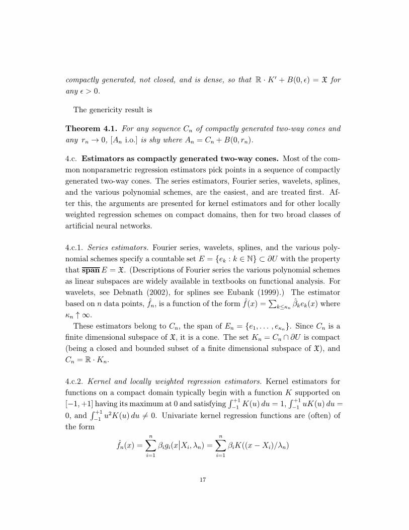
4.c. Estimators as compactly generated two-way cones. Most of the com-

mon nonparametric regression estimators pick points in a sequence of compactly

generated two-way cones. The series estimators, Fourier series, wavelets, splines,

and the various polynomial schemes, are the easiest, and are treated first. Af-

ter this, the arguments are presented for kernel estimators and for other locally

weighted regression schemes on compact domains, then for two broad classes of

artificial neural networks.

4.c.1. Series estimators. Fourier series, wavelets, splines, and the various poly-

nomial schemes specify a countable set E = ek : k ∈ N ⊂ ∂U with the property

that spanE = X. (Descriptions of Fourier series the various polynomial schemes

as linear subspaces are widely available in textbooks on functional analysis. For

wavelets, see Debnath (2002), for splines see Eubank (1999).) The estimator

based on n data points, fn, is a function of the form f(x) =∑k≤κn βkek(x) where

κn ↑ ∞.These estimators belong to Cn, the span of En = e1, . . . , eκn. Since Cn is afinite dimensional subspace of X, it is a cone. The set Kn = Cn ∩ ∂U is compact(being a closed and bounded subset of a finite dimensional subspace of X), and

Cn = R ·Kn.

4.c.2. Kernel and locally weighted regression estimators. Kernel estimators for

functions on a compact domain typically begin with a function K supported on

[−1,+1] having its maximum at 0 and satisfying ∫ +1−1 K(u) du = 1, ∫ +1−1 uK(u) du =0, and

∫ +1−1 u

2K(u) du 6= 0. Univariate kernel regression functions are (often) ofthe form

fn(x) =

n∑i=1

βigi(x|Xi, λn) =n∑i=1

βiK((x−Xi)/λn)

17

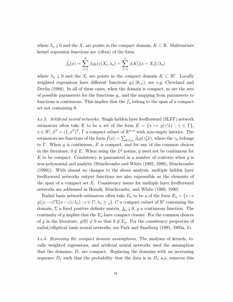
where λn ↓ 0 and the Xi are points in the compact domain, K ⊂ R. Multivariatekernel regression functions are (often) of the form

fn(x) =

n∑i=1

βigi(x|Xi, λn) =n∑i=1

βiK(‖x−Xi‖/λn)

where λn ↓ 0 and the Xi are points in the compact domain K ⊂ R`. Locallyweighted regressions have different functions gi(·|θi,n), see e.g. Cleveland andDevlin (1988). In all of these cases, when the domain is compact, so are the sets

of possible parameters for the functions gi, and the mapping from parameters to

functions is continuous. This implies that the fn belong to the span of a compact

set not containing 0.

4.c.3. Artificial neural networks. Single hidden layer feedforward (SLFF) network

estimators often take E to be a set of the form E = x 7→ g(γ′x) : γ ∈ Γ,x ∈ R`, xT = (1, xT )T , Γ a compact subset of Rn+1 with non-empty interior. Theestimators are functions of the form f(x) =

∑k≤κn βkg(γ

′kx), where the γk belongs

to Γ. When g is continuous, E is compact, and for any of the common choices

in the literature, 0 6∈ E. When using the Lp norms, g need not be continuous forE to be compact. Consistency is guaranteed in a number of contexts when g is

non-polynomial and analytic (Stinchcombe and White (1992, 1998), Stinchcombe

(1999)). With almost no changes to the above analysis, multiple hidden layer

feedforward networks output functions are also expressible as the elements of

the span of a compact set E. Consistency issues for multiple layer feedforward

networks are addressed in Hornik, Stinchcombe, and White (1989, 1990)

Radial basis network estimators often take En to be a of the form En = x 7→g((x− c)′Σ(x− c)/λn) : c ∈ C, λn ≥ n, C a compact subset of R` containing thedomain, Σ a fixed positive definite matrix, λn ↓ 0, g a continuous function. Thecontinuity of g implies that the En have compact closure. For the common choices

of g in the literature, g(0) 6= 0 so that 0 6∈ En. For the consistency properties ofradial/elliptical basis neural networks, see Park and Sandberg (1991, 1993a, b).

4.c.4. Removing the compact domain assumptions. The analyses of kernels, lo-

cally weighted regressions, and artificial neural networks used the assumption

that the domains, D, are compact. Replacing the domains with an increasing

sequence Dn such that the probability that the data is in Dn a.a. removes this

18

restriction. This adds a “with probability 1” qualification to the result that only

a shy set of functions are O(rn) approximable.

4.d. Interpretational issues. For a nonparametric technique X, a rate of con-

vergence result is of the form “Technique X can approximate any f in the set

F at a rate O(rn).” Theorem 4.1 implies that the set F that appear in such aconvergence result must be shy for any non-parametric regression scheme repre-

sentable as the countable union of compactly generated cones. However, it is still

possible that the reason that the set F must be shy is because the question is

being asked in “too large” a space X. The cost of shrinking the space X so that

the shyness result disappears is the loss of the strength in the consistency results

used to justify non-parametric regression analysis.

Theorem 4.1 applies when X is any separable Banach space. In particular,

imposing smoothness conditions by assuming that the target belongs to a Sobolev

space or to a space of m times continuously differentiable functions, Cm(X),

m ∈ N, X having a smooth boundary, does not change the conclusion. So, if itis the case that X is “too large,” it is either dimensionality or completeness that

is to blame.

Dimensionality: If the space X′ of all possible target functions is finite dimen-sional with a known basis, there is no reason to use non-parametric techniques.

If the finitely many basis functions are unknown, but belong to to some infinite

dimensional Banach space X, we are back in essentially the same situation —

convergence at any rate O(rn) can only be had if the basis functions belong to ashy set.

Completeness: The other possibility is that the space X′ of all possible targetfunctions is incomplete. The largest set of functions approximable at the rate

O(rn) by a nested sequence Cn of compactly generated two-way cones is theincomplete set X′ =

⋃M [Cn +B(0,M · rn) a.a.].

Lemma 4.2. If Cn =∑nk=1R · E(n), E(n) a nested, increasing sequence of

compact subsets of ∂U , and span E(n) : n ∈ N = X, then X′ = ⋃M [Cn +B(0,M · rn) a.a.] is incomplete and contains a dense, linear subspace.

19

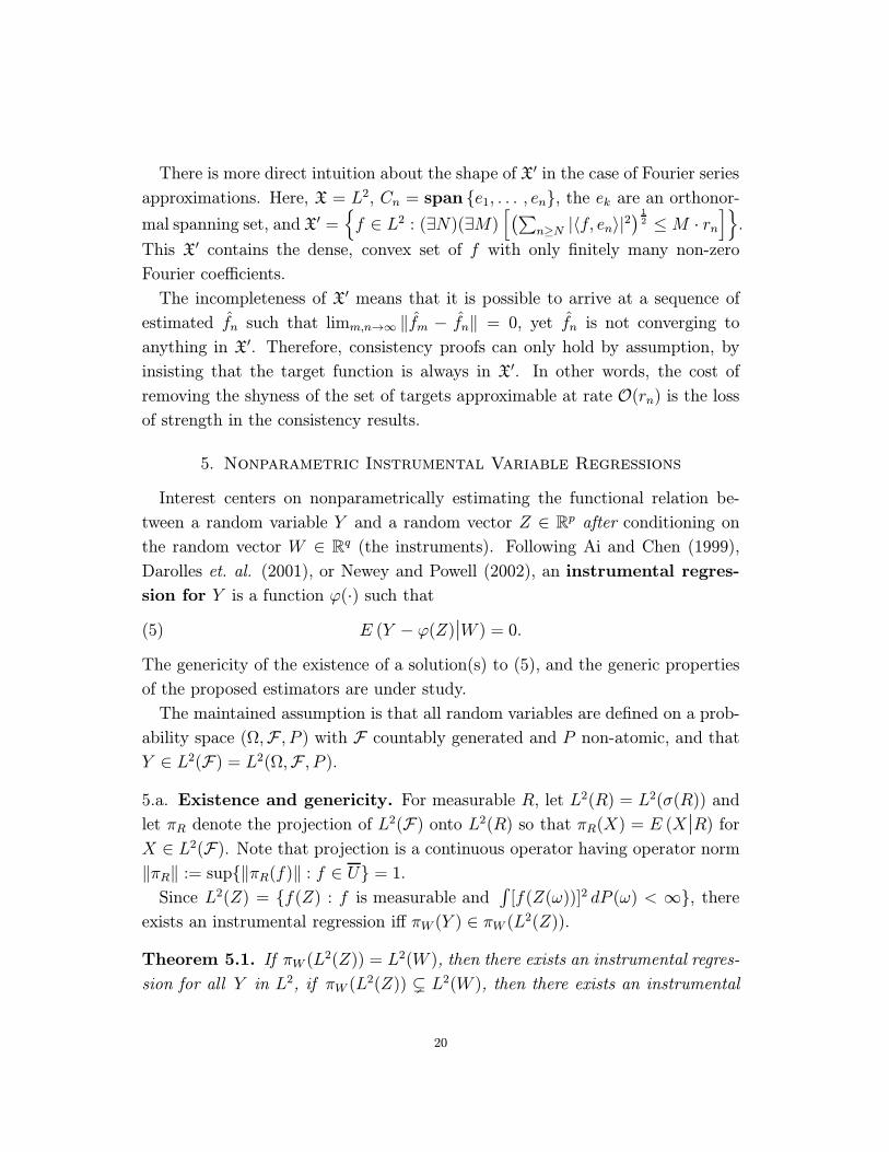
There is more direct intuition about the shape of X′ in the case of Fourier seriesapproximations. Here, X = L2, Cn = span e1, . . . , en, the ek are an orthonor-mal spanning set, and X′ =

f ∈ L2 : (∃N)(∃M)

[(∑n≥N |〈f, en〉|2

) 12 ≤M · rn

].

This X′ contains the dense, convex set of f with only finitely many non-zeroFourier coefficients.

The incompleteness of X′ means that it is possible to arrive at a sequence ofestimated fn such that limm,n→∞ ‖fm − fn‖ = 0, yet fn is not converging toanything in X′. Therefore, consistency proofs can only hold by assumption, byinsisting that the target function is always in X′. In other words, the cost ofremoving the shyness of the set of targets approximable at rate O(rn) is the lossof strength in the consistency results.

5. Nonparametric Instrumental Variable Regressions

Interest centers on nonparametrically estimating the functional relation be-

tween a random variable Y and a random vector Z ∈ Rp after conditioning onthe random vector W ∈ Rq (the instruments). Following Ai and Chen (1999),Darolles et. al. (2001), or Newey and Powell (2002), an instrumental regres-

sion for Y is a function ϕ(·) such thatE (Y − ϕ(Z)|W ) = 0.(5)

The genericity of the existence of a solution(s) to (5), and the generic properties

of the proposed estimators are under study.

The maintained assumption is that all random variables are defined on a prob-

ability space (Ω,F , P ) with F countably generated and P non-atomic, and thatY ∈ L2(F) = L2(Ω,F , P ).5.a. Existence and genericity. For measurable R, let L2(R) = L2(σ(R)) and

let πR denote the projection of L2(F) onto L2(R) so that πR(X) = E (X|R) for

X ∈ L2(F). Note that projection is a continuous operator having operator norm‖πR‖ := sup‖πR(f)‖ : f ∈ U = 1.Since L2(Z) = f(Z) : f is measurable and ∫ [f(Z(ω))]2 dP (ω) < ∞, thereexists an instrumental regression iff πW (Y ) ∈ πW (L2(Z)).Theorem 5.1. If πW (L

2(Z)) = L2(W ), then there exists an instrumental regres-

sion for all Y in L2, if πW (L2(Z)) ( L2(W ), then there exists an instrumental

20

regression only for Y belonging to a shy subset of L2, if πW (L2(Z)) ( L2(W ),

then there exists an instrumental regression only for Y belonging to a proper

closed subspace of L2.

The more difficult questions concern the genericity of the set of (W,Z) pairs

such that πW (L2(Z)) = L2(W ), or, for fixed W the genericity of the set of

instruments Z such that πW (L2(Z)) = L2(W ). If Z = W or if the vector Z

contains W as a subvector, then πW (L2(Z)) = L2(W ), but this case is hardly

interesting for instrumental variable regressions.

Lemma 5.1. The set R = X ∈ L2(F) : σ(X) = F is Baire large.For all (W,Z) pairs in the Baire large set R × R, σ(W ) = σ(Z) = F so that

L2(W ) = L2(Z) = L2(F). An immediate Corollary is the existence of a functionϕ such that Y = ϕ(W ). In other words, using Baire largeness gives the rather

odd conclusion that statistics is, generically, about the recovery of deterministic

relations between observables. I conjecture that the set R in Lemma 5.1 and the

set of (W,Z) pairs such that πW (L2(Z)) = L2(W ) are both shy.1

5.b. Generic properties of estimators. A maintained assumption in the es-

timators of ϕ in nonparametric instrumental regression is that πW is a compact

operator from L2(Z) to L2(W ) (e.g. Chen and Shen (1998), Ai and Chen (1999),

Darolles, Florens, and Renault (2001), Newey and Powell (2002)). Use of instru-

mental variables that contain information independent of the regressors is known

to be bad statistical practice.

Lemma 5.2. If πW is a compact operator from L2(Z) to L2(W ) and W does

not have finite range, then πW (L2(Z)) ( L2(W ). If some non-constant function

of W is independent of Z, then πW (L2(Z)) ( L2(W ).

Thus, consistency and rate results obtained using compact projection operators

apply only Y in a shy subset of L2(F), and the use of bad instruments leadsto non-existence of instrumental regressions unless Y belongs to a closed linear

subspace with no interior.

1This problem is geometrically miserable because σ(r ·X) = σ(X) for all r 6= 0. Therefore, theset of X such that dC(σ(X),F) = c is a cone without the origin where dC(·, ·) is any metric onsub-σ-fields. There seems to be no clear relation between the vector space structure of L2(F)and the properties of the sub-σ-fields by the elements of L2(F).

21

Suppose that no non-constant function of the regressors is independent of the

instruments. Even if one assumes, in order to have an easier estimation strategy,

that the Y belongs to a shy set, one should examine the primitive assumptions

used to guarantee that the projection be a compact operator. Of particular

interest is the role of an informational “continuity” assumption.

The variables (W,Z) may have components in common, let X = (X)ri=1 ∈ Rrdenote the random vector of components in (W,Z) after duplicates have been

removed. Let Q (resp. Qi) denote the distribution (resp. the i’th marginal distri-

bution) of X.

Definition 5.1. The information in Q is continuous if ×iQi Q, that is, if

there exists a measurable f ≥ 0 such that, for all E ∈ Br, Q(E) = ∫Ef d×iQi.

Generically, information is dis-continuous, and this is equivalent to the exis-

tence of a subtle kind of commonality among the components of X.

Let ∆(Rr) denote the set of distributions on Br, the Borel σ-field on Rr, and forI ⊂ 1, . . . , r, let BI denote the product σ-field generated by the i’th marginalsub-σ-fields, i ∈ I.Definition 5.2. A set B ∈ Br is Q-smooth if Q(B) > 0 and QB(·) := Q(·|B)is non-atomic. A Q-smooth B ∈ Br has measurable commonality if for non-empty, disjoint I, J ⊂ 1, . . . , r, there exists a measurable ψ : B → (0, 1] suchthat gI := EQB(ψ|BI) = gJ := EQB(ψ|BJ ) QB-a.e., and gI(QB) = gJ(QB) is

non-atomic. The probability Q has measurable commonality if there exists a

Q-smooth B ∈ B that has measurable commonality.Theorem 5.2. A prevalent subset of Q have dis-continuous information and

measurable commonality.

Measurable commonality means that there is some event B and some function ψ

on B such ψ(Q(·|B)) is non-atomic, and disjoint sets of components of the vectorX, I, J , such that conditioning on B and either of those sets of components

perfectly reveals the value of ψ. Given the generic equivalence of measurable

commonality and dis-continuous information, it is no surprise that the simplest

kind of measurable commonality is a diagonal concentration.

Example 5.1. With s and t independent and uniformly distributed on (0, 1], take

Q to be the distribution of (X1, X2) = (s, s) if s ∈ (0, 12 ] and (s, t) if s ∈ (12 , 1].

22

Let B be the event (s, s) ∈ (0, 12]× (0, 1

2], and define ψ = s on the set B to see

that Q has measurable commonality.

Stinchcombe (2002) provides more examples and an examination the role of

measurable commonality as conditional common knowledge in game theoretic

models.

5.c. Interpretational issues. It is possible that the shyness results for Y are

appearing because L2(F) is “too large.” When the instruments are badly chosen,this is clearly not the case. However, when the (W,Z) are such that the projection

operator is compact but has dense range, the set of Y for which an instrumental

regression exists is shy, but dense. Essentially the same arguments as appeared

in §4.d show that restricting attention to this dense set by assumption evisceratesthe strength of the consistency and rate of approximation results.

Finite dimensional questions are not interesting for nonparametric regression.

The situation is quite different for nonparametric instrumental variable regres-

sions. The subspaces L2(W ) and L2(Z) are finite dimensional iff W and Z have

finite range. Let P(W ) and P(Z) denote partitions of Ω generated by σ(W ) and

σ(Z) respectively. There are two observations:

1. An instrumental regression exists iff the columms of the #P(Z) × #P(W )matrix M = (P (A|B))A∈P(Z), B∈P(W ) are linearly independent (this is animplication of Theorem 5.1, but much more direct proofs can be found in

Newey and Powell (2002), Darolles et. al. (2001)). A necessary condition for

this is that Z take on at least as many values as W .

2. The existence of a non-constant function of W that is independent of Z

corresponds to the existence of at least 2 columns of non-zero constants in

M (a failure of the linear independence condition).

6. The Generic Consistency of ICM Tests

Under study are the generic properties of integrated conditional moment (ICM)

tests of regression specification, and ICM tests of conditional and unconditional

distributional specifications. ICM tests can be understood as estimators of the

continuous seminorm of a function ε, typically a residual. If the estimated value of

the seminorm is too large, the null hypothesis of correct specification is rejected.

23

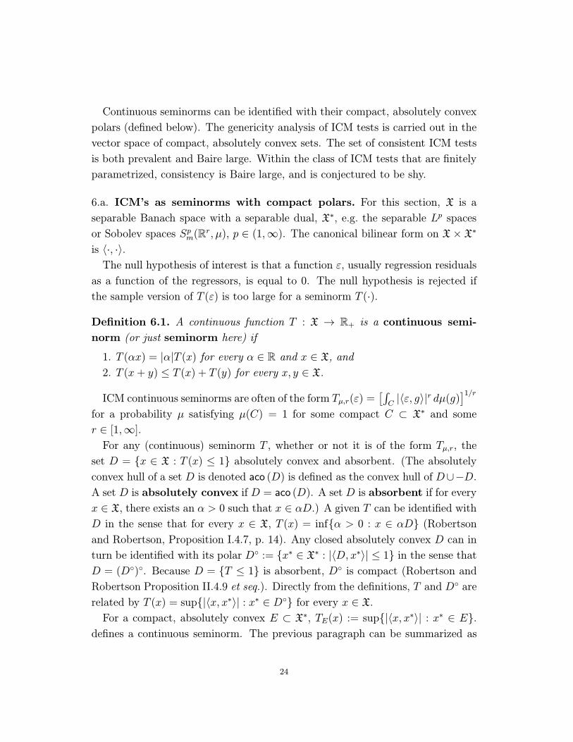
Continuous seminorms can be identified with their compact, absolutely convex

polars (defined below). The genericity analysis of ICM tests is carried out in the

vector space of compact, absolutely convex sets. The set of consistent ICM tests

is both prevalent and Baire large. Within the class of ICM tests that are finitely

parametrized, consistency is Baire large, and is conjectured to be shy.

6.a. ICM’s as seminorms with compact polars. For this section, X is a

separable Banach space with a separable dual, X∗, e.g. the separable Lp spacesor Sobolev spaces Spm(R

r, µ), p ∈ (1,∞). The canonical bilinear form on X× X∗is 〈·, ·〉.The null hypothesis of interest is that a function ε, usually regression residuals

as a function of the regressors, is equal to 0. The null hypothesis is rejected if

the sample version of T (ε) is too large for a seminorm T (·).

Definition 6.1. A continuous function T : X → R+ is a continuous semi-norm (or just seminorm here) if

1. T (αx) = |α|T (x) for every α ∈ R and x ∈ X, and2. T (x+ y) ≤ T (x) + T (y) for every x, y ∈ X.

ICM continuous seminorms are often of the form Tµ,r(ε) =[∫C|〈ε, g〉|r dµ(g)]1/r

for a probability µ satisfying µ(C) = 1 for some compact C ⊂ X∗ and somer ∈ [1,∞].For any (continuous) seminorm T , whether or not it is of the form Tµ,r, the

set D = x ∈ X : T (x) ≤ 1 absolutely convex and absorbent. (The absolutelyconvex hull of a set D is denoted aco (D) is defined as the convex hull of D∪−D.A set D is absolutely convex if D = aco (D). A set D is absorbent if for every

x ∈ X, there exists an α > 0 such that x ∈ αD.) A given T can be identified withD in the sense that for every x ∈ X, T (x) = infα > 0 : x ∈ αD (Robertsonand Robertson, Proposition I.4.7, p. 14). Any closed absolutely convex D can in

turn be identified with its polar D := x∗ ∈ X∗ : |〈D, x∗〉| ≤ 1 in the sense thatD = (D). Because D = T ≤ 1 is absorbent, D is compact (Robertson andRobertson Proposition II.4.9 et seq.). Directly from the definitions, T and D arerelated by T (x) = sup|〈x, x∗〉| : x∗ ∈ D for every x ∈ X.For a compact, absolutely convex E ⊂ X∗, TE(x) := sup|〈x, x∗〉| : x∗ ∈ E.defines a continuous seminorm. The previous paragraph can be summarized as

24

saying “T is a continuous seminorm iff it is of the form TD withD being compact

and absolutely convex.”

For the ICM seminorms Tµ,r, we have

Lemma 6.1. If C is a compact subset of X∗, and µ is a probability measure onX∗ with µ(C) = 1, then for each r ∈ [1,∞], there exists an absolutely convexsubset Er ⊂ aco (C) such that for all x ∈ X, TEr(x) = Tµ,r(x).The class of compact absolutely convex subsets of X∗ is denoted K. Additionand scalar multiplication of elements of K are continuous in the Hausdorff metric,

dH , and (K, dH) is a complete, separable locally convex topological vector space.

Definition 6.2. A test E ∈ K is consistent if ⋂r>0x ∈ X : TE(x) < r = 0.The equivalence of the following comes directly from standard concepts in the

study of topological vector spaces: E is consistent; the seminorm topology gen-

erated by E is Hausdorff; the span of E is σ(X∗,X) dense in X∗ (see Stinchcombeand White (1998) for details).

Generically, ICM tests are consistent.

Theorem 6.1. The set of consistent E ∈ K is prevalent and Baire large.6.b. Examples. Many tests of the correctness of parametric specification of re-

gression models, most tests of the equality of unconditional distributions and

of the equality of parametrized conditional distributions can be formulated as

estimators of a TE, E ∈ K.6.b.1. Tests of parametric regression models. A parametric model for a condi-

tional mean is a collection of functions on R`, x 7→ f(x, θ) : θ ∈ Θ, x ∈ R`,Θ ⊂ Rk. The null hypothesis that the model is correctly specified for E(Y |X) is

H0 : (∃θ0 ∈ Θ)[u = Y − f(X, θ0), and ε = E(u|X) = 0)].(6)

Pick p, q ∈ (1,∞) such that 1p+ 1q= 1. The set of deviations, ε, from the

null is Lp(X) := Lp(Ω, σ(X), P ) with σ(X) being the minimal σ-field making X

measurable. Specifically, the set of possible deviations from H0 is

ε ∈ Lp(X) : (∃Y ∈ Lp(Ω,F , P ))[ε ∈ E(Y − f(X,Θ)|X)].(7)

The set of test functions is Lq(X). The literature has used sample versions of

TE for many E ∈ K.

25

1. If E = [−f, f ] = aco (f), f a function in Lq(X), Hausmann (1978), Newey(1985), Tauchen (1985), White (1987), White (1994). Such tests are not con-

sistent, having no power against anything in the “orthogonal” complement

of E.

2. ForX taking values in compact subsets of R`, ` ≥ 1, Bierens (1990) analyzesE = aco (x 7→ exp(x′τ) : τ ∈ T), T a compact cube in R`.

3. Again for X taking values in compact subsets of R`, Stinchcombe and White

(1998) analyzes E = aco (x 7→ f(x′τ) : τ ∈ T), T a compact subset ofR`+1 with non-empty interior, where x = (1, x′)′ ∈ R`+1, and f is any non-polynomial analytic function.

4. For X ∈ R1, Stute (1997) analyzes E = aco (x 7→ 1(−∞,a](x) : a ∈ R).By Lemma 6.1, the class of TE also contains ICM tests of Bierens (1982),

Bierens (1990), White (1989), Stinchcombe and White (1998), and Bierens and

Ploberger (1997). Theorem 6.1 shows that, in the class of all ICM tests for correct

specification, the consistent ones are generic.

6.b.2. Tests of the equality of unconditional distributions. The null hypothesis

for the Kolmogorov-Smirnov test is the the equality of two distributions on [0, 1]

with Lebesgue densities f and h. The densities f and h are elements of X =

Lp([0, 1],B, λ), p ∈ (1,∞), B being the usual Borel sets λ being Lebesgue measure.The null hypothesis is that ε := f − h = 0 where f, h ∈ C, C the convex, normclosed set of densities. The set of deviations from the null hypothesis is the set

C − C. The test functions belong to Lq([0, 1],B, λ), 1p+ 1q= 1.

When E is the compact subset of Lq, aco (1[0,a](·) : a ∈ (0, 1)), the sampleversion of TE(ε) = supx∗∈E |〈ε, x∗〉| is the Kolmogorov-Smirnov statistic. If F nand Hn are empirical cdf’s from two iid. samples drawn with densities f and h,

the sample version of the statistic is supa∈(0,1) |F n(a)−Hn(a)|.The Cramer-von Mises test for ε = 0 is the the sample version of

Tµ,2(ε) =

[∫C

|〈ε, x∗〉|2 dµ(x∗)] 12

(8)

where µ is the compactly supported distribution on X∗ induced by picking ana ∈ [0, 1] according to the uniform distribution and then integrating ε againstx∗ = 1[0,a]. Note that C is a compact subset of Lq, and by Lemma 6.1, there is aE ⊂ aco (C) such that TE(ε) = Tµ,2(ε) for all ε ∈ Lp.

26

Theorem 6.1 implies that for generic E, the test based on sample versions of

TE is consistent.

6.b.3. Tests for parametric specifications of conditional distributions. This fol-

lows Andrews (1997) and Stinchcombe andWhite (1998). Let the conditional like-

lihood function with respect to a σ-finite measure ν and parameterized by θ ∈ Θ,Θ an open subset of Rp, be given by a measurable function, f : R×Rk×Θ→ R+,with the property that for all x ∈ Rk and θ ∈ Θ, ∫

Rf(y|x, θ)dν(y) = 1. Let S

denote f(·|·, θ) : θ ∈ Θ. S is correctly specified for Y conditional on Xwhen for PX-almost all x, f(·|x, θ0) is a version of the true conditional density ofY given X = x with respect to ν for some θ0 in Θ.

For θ ∈ Θ, define Qθ to be the distribution on R1 ×R`,

Qθ(A) =

∫A

f(y|x, θ) dν(y)dPX(x), A a Borel subset of R× Rk.(9)

With P denoting the true distribution of (Y,X), the null hypothesis is that

0 ∈ P − Qθ : θ ∈ Θ.Assume that P has a density with respect to ν × PX . This is not innocuous,but it is a minimal assumption needed for entertaining the possibility that the

model is correctly specified. A space containing the densities of P and the Qθ is

X = Lp(R1+`,B1+`, ν × PX),(10)

p ∈ (1,∞). The test functions belong to the dual space X∗ = Lq. Stinchcombe

and White (1998) used E = aco (x 7→ f(x′γ) : γ ∈ Γ), Γ a compact subset ofR`+1 with non-empty interior, f any non-polynomial analytic function. Andrews

(1997) uses the Lq compact set E = aco (1(−∞,z](·) : z ∈ Z) where Z is asupport set for the random vector (Y,X) in R1+`.

Theorem 6.1 implies that for generic E, the test based on sample versions of

TE is consistent.

6.c. Finitely parametrized ICM’s. As seen in the examples, the E that arise

in practice are often smoothly parametrized by finite dimensional sets. Such E

are the smooth images of a compact Θ.

This section supposes that Θ is an infinite, compact metric space. Let C(Θ;X)

denote the set of continuous functions from Θ to a separable Banach space X. A

vector subspace C ′ ⊂ C is full if for all finite collections θn : n ≤ N ⊂ Θ, and

27

all collections hn : n ≤ N ⊂ X, there exists an f ∈ C ′ such that f(θn) = hn

for n ≤ N . When Θ is a manifold, the vector subspaces of smooth functions

in C(Θ;X) are typically full, typically dense, and they are typically Gδ’s, hence

topologically complete.

Theorem 6.2. If Θ is a compact metric space, and C ′ is a dense, full vectorsubspace that is a Gδ in C(Θ;X), then the set f ∈ C ′ : aco (f(Θ)) is consistentis Baire large in C ′.

I conjecture that this result is true with “prevalent” replacing “Baire large,”

but this is an open (and vexing) problem.

For Θ an infinite compact space, C ′ = C(Θ;X) satisfies the remaining assump-tions in Theorem 6.2. This means that for any infinite, compact parameter set,

a dense set of continuous parametrizations spans X. In some directions, this is a

generalization of the universal approximation results for neural networks in Cy-

benko (1989), Funahashi (1989), Hornik, Stinchcombe and White (1989, 1990).

6.d. Interpretational issues. It is possible that the conclusion that the set of

consistent ICM’s being “large” is due to the problem being imbedded in “too

small” a set of ICM tests. However, it seems quite difficult to imagine a larger

space of non-adaptive tests than the space K considered here.

7. Concluding Remarks

A genericity analysis becomes nonsensical if the wrong setting is chosen — if the

statistically relevant cases are two dimensional, then a three dimensional generic-

ity analysis hides more than it reveals. The challenge then, is to understand the

results found here in this light.

Bayesian updating: The generic inconsistency of Bayes updating in plausible

infinite contexts is surprising. Small details of the prior turn out to matter quite

sharply. It seems to mean that we should calculate out which observation(s) have

the most effect on our posterior distribution and ask if we trust those data enough

to tolerate them moving the posterior as much as they do. There are a number

of possible heuristics for these procedures, but almost certainly there is no best

procedure.

Limiting the set of priors can, in many cases, provide computationally tractable,

parametrized statistical models. As a general model of optimizing behavior, such

28

a step is clearly unsatisfactory. Further, even in these parametrized models,

Bayesian updating can be inconsistent. These considerations lead to the conclu-

sion that the genericity of inconsistency is not an artifact of the wrong setting

being chosen.

Nonparametric regression: Rates of convergence analyses are, hopefully, guides

to finite sample behavior. Quick rates of convergence are often achieved at the

expense of maintaining smoothness assumptions. It is difficult to give a satisfac-

tory general argument about e.g. the appropriateness of smoothness conditions

that improve rates. For example, if the errors in the X’s in a non-linear regression

are plausibly smoothly distributed, the best possible recoverable mean of the Y

conditional on observed X is likely to be a smooth function, whether or not the

true conditional mean is. The present work shows that whatever the smoothness

assumptions are, they do not cover a generic set of targets. If one is not willing

to firmly declare for a non-generic set, then rate of convergence results only hold

at the expense of consistency results.

One version of the lessons to be drawn from the genericity analysis of nonpara-

metric regression is that technique without insight will not carry us very far. By

being “without insight” into a particular regression function, I mean that “all of

X must be considered.” The results here reinforce the lesson that X is a very

large place to search.

Instrumental variable regressions: The analysis of nonparametric instrumental

regressions reinforces one’s convictions that it is a difficult business. The required

assumptions are generically not satisfied under the known conditions needed for

estimation, and the target regression functions are, generically, not fully recover-

able. In particular, there is a clear formulation of functional relations not being

recoverable if the instruments are badly chosen.

A further benefit of the present analysis is that it shows that one of the non-

generic required assumptions is equivalent to there being no measurable com-

monality. Measurable commonality is generically equivalent to dis-continuous

information. This provides a bit more shape to the question of whether the

continuous information assumption is acceptable.

Specification testing: Once Bierens (1982, 1990) gave us the initial insights,

consistent ICM tests became relatively easy to write down. The results here

suggest that we should not be surprised by this because consistency is a generic

29

property of ICM tests. This is so pleasant a conclusion that I cannot find it in

myself to question whether it arises from wrong-headedness.

8. References

Ai, Chunrong and Xiaohong Chen (1999). “Efficient Estimation of Models withConditional Moment Restrictions Containing Unknown Functions”, working paper,University of Florida and London School of Economics.

Anderson, Robert M. and William R. Zame (2001). “Genericity with Infinitely ManyParameters,” Advances in Theoretical Economics: Vol. 1: No. 1, Article 1.

Andrews, Donald W. (1997). “A Conditional Kolmogorov Test. Econometrica,” 65,1097-1128.

Arnold, Barry C., Patrick L. Brockett, William Torrez, and A. Larry Wright (1984).“On the Inconsistency of Bayesian Non-Parametric Estimators in Competing Risk/-Multiple Decrement Models,” Insurance, Mathematics and Economics, 3, 49-55.

Baire, Rene. (1899). “Sur les Fonctions de Variables Reelles,” Annali di MatematicaPura ed Applicada Series 3, Vol. 3, 1-122.

Bierens, Hermann B. (1982). “Consistent Model Specification Tests,” Journal ofEconometrics, 20, 105-134.

Bierens, Hermann B. (1990). “A Consistent Conditional Moment Test of FunctionalForm,” Econometrica 58, 1443-1458.

Bierens, Hermann B. and Werner Ploberger (1997). “Asymptotic Theory of Inte-grated Conditional Moment Tests.” Econometrica, 65, 1129-1152.

Chen, X. and X. Shen (1998). “Sieve Extremum Estimates for Weakly DependentData,” Econometrica, 66, 289-314.

Christensen, Jens Peter Reus (1974). Topology and Borel Structure. Amsterdam:North-Holland Publishing Company.

Cleveland, William and Susan Devlin (1988). “Locally Weighted Regression: AnApproach to Regression Analysis by Local Fitting,” Journal of the American Sta-tistical Association, 83(403), 596-610.

Cybenko, G. (1989). “Approximation by Superpositions of a Sigmoidal Function.”Mathematics of Control, Signals and Systems 2, 303-14.

Cotter, Kevin D. (1986). “Similarity of Information and Behavior with a PointwiseConvergence Topology.” Journal of Mathematical Economics 15(1) 25-38.

30

Darolles, Serge, Jean-Pierre Florens, and Eric Renault (2001). “Nonparametric In-strumental Regression,” Manuscript, GREMAQ, University of Toulouse.

Dellacherie, C. and P.-A. Meyer (1978), Probabilities and Potential. Amsterdam:North Holland Publishing Co.

Diaconis, Persi and David Freedman (1986a). “On the Consistency of Bayes Esti-mates,” Annals of Statistics 14(1), 1-26.

Diaconis, Persi and David Freedman (1986b). “On Inconsistent Bayes Estimats ofLocation,” Annals of Statistics 14(1), 68-87.

Eubank, Randall L. (1999). Spline smoothing and nonparametric regression, 2’nd ed.M. Dekker, New York.

Ferguson, T. (1973). “A Bayesan Analysis of Some Nonparametric Problems,” Annalsof Statistics 1, 209-230.

Freedman, David (1963). “On the Asymptotic Behavior of Bayes Estimates in theDiscrete Case I,” Annals of Mathematical Statistics 34, 1386-1403.

Freedman, David (1965). “On the Asymptotic Behavior of Bayes Estimates in theDiscrete Case II,” Annals of Mathematical Statistics 36, 454-456.

Funahashi, K. (1989). On the Approximate Realization of Continuous Mappings byNeural Networks. Neural Networks 2, 183-92.

Grenander, Ulf (1981). Abstract Inference. Wiley, New York.

Halmos, Paul (1957). Introduction to Hilbert space and the theory of spectral multi-plicity, 2’nd ed. Chelsea Pub. Co., New York.

Hausman, J. (1978). “Specification Tests in Econometrics,” Econometrica 46, 1251-1272.

Hornik, Kurt (1991). “Approximation capabilities of multilayer feedforward net-works,” Neural Networks 4(2), 251-257.

Hornik, K. (1993). “Some New Results on Neural Network Approximation,” NeuralNetworks 6(8), 1069-1072.

Hornik, Kurt, Maxwell Stinchcombe, and Halbert White (1989). “Multi-layer Feed-forward Networks are Universal Approximators,” Neural Networks 2, 359-366 (1989).

Hornik, Kurt, Maxwell Stinchcombe, and Halbert White (1990). “Universal Approx-imation of an Unknown Mapping and its Derivatives using Multilayer FeedforwardNetworks,” Neural Networks 3, 551-560 (1990).

Hunt, B. R., T. Sauer, and J. A. Yorke (1992). “Prevalence: A Translation-Invariant‘Almost Every’ on Infinite-Dimensional Spaces,” Bulletin (New Series) of the Amer-ican Mathematical Society 27, 217-238.

31

Debnath, Lokenath (2002). Wavelet transforms and their applications. Birkhauser,Boston.

Nachbar, John (1997). “Prediction, Optimization, and Learning in Repeated Games,”Econometrica, 65(2), 275-309.

Newey, Whitney (1985). “Maximum Likelihood Specification Testing and ConditionalMoment Tests,” Econometrica 53, 1047-70.

Newey, Whitney and James Powell (2002). “Instrumental Variable Estimation ofNonparametric Models,” forthcoming, Econometrica.

Park, J. and I. W. Sandberg (1991). “Universal Approximation Using Radial Basis-Function Networks,” Neural Computation, 3(2), 246-257.

Park, J. and I. W. Sandberg (1993a). “Approximation and Radial-Basis FunctionNetworks,” Neural Computation, 5(2), 305-316.

Park, J. and I. W. Sandberg (1993b). “Nonlinear Approximations Using EllipticBasis Function Networks,” Circuits, Systems and Signal Processing, 13(1), 99-113.

Robertson, Alex P. and Wendy J. Robertson (1973). Topological Vector Spaces. Cam-bridge University Press, Cambridge.

Rudin, Walter (1973). Functional Analysis. McGraw-Hill, New York.

Stinchcombe, Maxwell (1990). “Bayesian Information Topologies,” Journal of Math-ematical Economics 19, 3, 233-254.

Stinchcombe, Maxwell (1993). “A Further Note on Bayesian Information Topologies,”Journal of Mathematical Economics 22, 189-193.

Stinchcombe, Maxwell (1999). “Neural Network Approximation of Continuous Func-tionals and Continuous Functions on Compactifications,” Neural Networks 12, 467-477.

Stinchcombe, Maxwell (2001). “The Gap Between Probability and Prevalence: Lone-liness in Vector Spaces,” Proceedings of the American Mathematical Society 129,451-457.

Stinchcombe, Maxwell (2002). Finiticity in Measurable-Continuous Games. Depart-ment of Economics, University of Texas at Austin.

Stinchcombe, Maxwell and Halbert White (1992). “Using Feedforward Networks toDistinguish Multivariate Populations,” with Halbert White, Proceedings of theInternational Joint Conference on Neural Networks, IEEE Press, New York, I:788-793.

Stinchcombe, Maxwell and Halbert White (1998). “Consistent Specification Test-ing with Nuisance Parameters Present Only Under the Alternative,” EconometricTheory 14, 295-325.

32

Stute, W. (1997). Nonparametric Model Checks for Regression. Annals of Statistics,Vol. 25, 613-641.

Tauchen, G. (1985). “Diagnostic Testing and Evaluation of Maximum LikelihoodModels,” Journal of Econometrics 30, 415-444.

White, Halbert (1987). “Specification Testing in Dynamic Models,” in T. Bewley,(ed.), Advances in Econometrics - Fifth World Congress, Vol 1. New York: Cam-bridge University Press, pp. 1-58.

White, Halbert (1989). “An Additional Hidden Unit Test for Neglected Nonlinear-ity in Multilayer Feedforward Networks,” Proceedings of the International JointConference on Neural Networks, Washington D.C.. San Diego: SOS Printing,II:451-455.

White, Halbert (1994). Estimation, Inference and Specification Analysis. CambridgeUniversity Press, New York.

9. Proofs

Proof of Lemma 2.1: The equivalence of (1) and (2) is immediate. Thefollowing proof of the equivalence of (1) and (3) is directly from Hunt, Sauer, andYorke (1992), and is reproduced here for completeness.If Λk(S) = 0, take η = Uk, the uniform distribution on [0, 1]k. If there is a com-pactly supported η such that η(S+x) ≡ 0, then ∫

Rkη(S+x) dΛk(x) = 0, so that∫

Rk

[∫Rk1(S+x)(y) dη(y)

]dΛk(x) = 0, implying

∫Rk

[∫Rk1(S+x)(y) dΛ

k(x)]dη(y) =

0. Since 1(S+x)(y) ≡ 1(S−y)(x) and∫Rk1(S−y)(x) dΛk(x) = Λk(S − y), we have∫

RkΛk(S − y) dη(y) = 0. Since Λk is translation invariant and non-negative,

Λk(S − y) ≡ Λk(S) ≥ 0, ∫RkΛk(S) dη(y) = 0, implying that Λk(S) = 0.

Proof of Lemma 2.3: If necessary, translate C so that 0 ∈ rel intcoS(coS). Foreach n ∈ N, [n · coS]∩C is a closed set with no interior in the csm space C. ByBaire’s theorem, the complement of ∪n[n ·coS]∩C is residual, hence non-empty.Pick arbitrary v in this residual set, and take η to be the uniform distribution onthe line Lv = [0, v].For any x ∈ X, [Lv + x] ∩ coS is a compact convex interval, possibly emptyor degenerate. Suppose, for the purposes of contradiction, that this interval haspositive η mass. This means that it is a line segment [y, y′], y 6= y′. Since0 ∈ rel intcoS(coS) and coS is convex, there exist ky, ky′ > 0 such that −ky ·y,−ky′ · y′ ∈ coS. Therefore, the plane spanned by [Lv +x]∩ coS and 0 belongsto ∪n[n · coS] ∩ C. But v also belongs to this set, a contradiction.Proof of Theorem 3.1: Fix a full support θ and a countable collection offn ∈ Cλ++ such that the θn := θfn are dense in ∆(X), and θn 6= θ for all n ∈ N.

33

Abuse notation with fn(ht) := Πti=1fn(xi) for partial histories h

t = (x1, . . . , xt).Let Un,m be a nested sequence of open neighborhoods of θn with the diameter ofUn,m less than 1/m. Let vn,m : ∆(X) → [0, 1] be a continuous function takingthe value 1 on Un,m and 0 on the complement of Un,m−1. For each ht, define thecontinuous function mn,m(·, ht) on MλB by

mn,m(µ, ht) = (

∫Cλ+

vn,m(f)f(ht) dµ(f))/(

∫Cλ+

f(ht) dµ(f)).

This is the expected value of vn,m conditional on ht when beliefs are µ. If posterior

beliefs along a sequence of histories ht converge to δθn , then limtmn,m(µ, ht) = 1.

For ε > 0 and t ∈ N, define Sn,m(ε, t) = µ ∈ MλB :∫X∞mn,m(µ, h

t) dθ∞(ht) ≤ε. By continuity, Sn,m(ε, t) is a closed subset of MλB.Outline:

1. For all ε > 0 and for all t, Sn,m(ε/2, t) ⊂ coSn,m(ε/2, t) ⊂ Sn,m(ε, t). Thisintermediate result leads to

2. For all T ,⋂t≥T Sn,m(ε, t) is shy, equivalently,

⋃t≥T Sn,m(ε, t)

c is prevalent.3. err(θ) =

⋂ε,n,m,T

⋃t≥T Sn,m(ε, t)

c (the intersection taken over rational ε in

(0, 1)). Since the intersection of countably many prevalent sets is prevalent,this and the second step complete the proof.

Details:

1. For all ε > 0 and all t, S(ε/2, t) ⊂ coS(ε/2, t) ⊂ S(ε, t).Since each S(ε, t) is closed, showing coS(ε/2, t) ⊂ S(ε, t) is sufficient.Pick µ, µ′ ∈ S(ε/2, t) and 0 < α < 1. Let µαµ′ = αµ + (1 − α)µ′. Whatmust be shown is

∫m(µαµ′, ht) dθ∞(ht) ≤ ε. For numbers s, s′ > 0 and

r, r′ ≥ 0 αr+(1−α)r′αs+(1−α)s′ ≤ max rs , r

′s′ ≤ r

s+ r′s′ . This delivers∫

m(µαµ′, ht) dθ∞(ht)

=

∫ ∫vn,m(f)f(h

t) dµαµ′(f)∫f(ht) dµαµ′(f)

dθ∞(ht)

≤∫ ∫

vn,m(f)f(ht) dµ(f)∫

f(ht) dµ(f)dθ∞(ht) +

∫ ∫vn,m(f)f(h

t) dµ′(f)∫f(ht) dµ′(f)

dθ∞(ht)

≤ ε/2 + ε/2 = ε,

completing the proof of the first step.2. For all T ,

⋂t≥T Sn,m(ε, t) is shy.

We have⋂t≥T Sn,m(ε, t) ⊂

⋂t≥T coSn,m(ε, t) ⊂

⋂t≥T Sn,m(2ε, t). by the

definition of co and Step 1. The set⋂t≥T coSn,m(ε, t) is convex and closed.

34

Therefore, it is sufficient to show that the closed set⋂t≥T Sn,m(2ε, t) has no

interior. The proof will be completed by showing the existence of a denseset Dn with the property that Dn ∩

⋂t≥T Sn,m(ε, t) = ∅. Specifically, the set

Dn will have the property that for every µ ∈ Dn, µ(·|ht)→w∗ δθn θ∞-a.e.Let M ⊂ M denote the set of probabilities for which there exists somenon-empty open set in ∆(X) receiving mass 0. Let Dn be the set of µ’s inMλB putting positive mass on θn and on finitely many points in M . Dn iseasily seen to be dense. Since θ is full support, every non-empty open setwill be visited infinitely often θ∞ a.e. Therefore, for every µ ∈ Dn, onlythe full support θn can have positive posterior weight in the limit, that is,µ(·|ht)→w∗ δθn .

3. err(θ) =⋂ε,n,m,T

⋃t≥T Sn,m(ε, t)

c (the intersection taken over rational ε in

(0, 1)).Since the θn are dense in ∆(X) and the diameters of the Un,m con-verge to 0, every non-empty open U contains a Un,m. Therefore, µ ∈⋂ε,n,m,T

⋃t≥T Sn,m(ε, t)

c iff for all rational ε in (0, 1), all non-empty open

U , and all T , there exists a t ≥ T such that µ 6∈ Sn,m(ε, t), that is, iffµ ∈ err(θ).

Proof of Lemma 4.1: Let xn = rn ·kn, kn ∈ K ′, be a sequence in the compactlygenerated two-way cone C = R · K ′, K ′ a compact subset of ∂U , and supposethat ‖xn − x‖ → 0. Then rn := ‖xn‖ → ‖x‖, and kn → k for some k ∈ K ′.Therefore x = ‖x‖k ∈ R ·K ′, so that C is closed.Suppose that C = R · K for some compact K ⊂ ∂U . Let F be closed andsuppose that ‖F‖ ≤ B. Then C ∩F is closed by the first step. Further, C ∩F ⊂[−B,B] ·K ∩F expresses C ∩F as a closed subset of the compact set [−B,B] ·Kso that C ∩ F is compact.If C ∩ F is compact for every closed, norm bounded F , then K ′ := C ∩ ∂U iscompact, and C = R ·K ′.Finally, if C has non-empty interior, then C ∩ U has non-empty interior. But

C ∩ U is compact, and compact subsets of X must have empty interior.Proof of Theorem 4.1: Fix arbitrary R > 0. Taking the union over somesequence Rn ↑ ∞ shows that it is sufficient to prove that (R ·U)∩ [An i.o.] is shy.Fix arbitrary ε > 0. R·U is a subset of the closed, norm bounded set R·(1+ε)U .For each n, let Fn be the compact, hence approximately flat set Cn∩(R ·(1+ε)U).By Lemma 2.2, S = [(Fn + B(0, rn)) i.o.] is shy. By construction, [(R · U) ∩[An i.o.]] ⊂ S.

Proof of Lemma 4.2: X′ contains the dense set⋃nCn. The completion of a

dense subset of any complete metric space is the space itself. Therefore, if X′ wascomplete, it would be equal to X, which contradicts Theorem 4.1.

35

If f, g ∈ ⋃n Cn, there there exists an N such that f, g ∈ CN . Since CN is atwo way cone, for all α, β ∈ R, αf, βg ∈ CN =

∑Nk=1R · Ek. Since EN ⊂ E2·N ,

αf + βg ∈ C2·N ⊂⋃nCn.

Proof of Theorem 5.1: If S = πW (L2(Z)) ( L2(W ), then it is immediate thatthe only Y for which an instrumental regression can exist belong to the closed,

proper subspace π−1W (S)), proving the last part of the Theorem.Now treat πW as a continuous operator from L2(Z) to L2(W ) (it still hasoperator norm 1), and suppose that πW (L

2(Z)) ( L2(W ). There are two cases,when πW is bounded below, inf‖πW (f)‖ : f ∈ L2(Z) ∩ ∂U = δ > 0, andinf‖πW (f)‖ : f ∈ L2(Z) ∩ ∂U = 0.When πW is bounded below, it is invertible on the closure of its range (e.g.Halmos (1957, p. 38)), implying that the range is closed. A closed proper subspaceof L2(W ) is shy, completing the proof in this case.If inf‖πW (f)‖ : f ∈ L2(Z) ∩ ∂U = 0, then there exists a sequence fn ∈

L2(Z) ∩ ∂U such that ‖πW (fn)‖ → 0. Let N = span fn : n ∈ N. ExpressingL2(Z) as the direct sum N⊥⊕N shows that πW (L2(Z)) ⊂ (πW (N))⊥⊕πW (N). Forany shy set S, S⊥⊕S is shy, so it is sufficient to show that πW (N) is a shy subsetof L2(W ). For this, it is in turn sufficient to show that πW (N) is a countableunion of compact sets.N ∩U is a weakly compact subset of L2(Z), so it is sufficient to show that, re-stricted to N, πW is a compact operator (i.e. continuous when the range, L

2(W ), isgiven the norm topology and the domain, N ⊂ L2(Z), is given the weak topology).This follows from ‖πW (fn)‖ → 0.Proof of Lemma 5.1: The relevant metric on sub-σ-fields is

dC(H,G) =∑n∈N2−nmin1, ‖E (fn|H)− E (fn|G)‖(11)

where fn is a countable dense subset of L2(F). This metric and its basic properties

are due to Cotter (1986), the Bayesian interpretation of this metric can be foundin Stinchcombe (1990, 1993). Basic properties of projections show that for anyr > 0, Sr+ = X ∈ L2(F) : dC(σ(X),F) ≥ r is closed, so that its complement,Sr−, is open. R =

⋂ε Sε−, so it is sufficient to show that each Sε− is dense in

L2(F).Pick arbitrary g ∈ L2(F) and ε > 0. It is sufficient to show that there existsan f such that ‖f − g‖ < ε and dC(σ(f),F) < ε.Enumerate a countable field F generating F as En : n ∈ N. Let Fn =

σEk : k ≤ n. dC(Fn,F) ↓ 0. Pick N1 such that dC(FN1,F) < ε.

Define g−n =∑k∈Z

k2n1f−1([k/2n,(k+1)/2n)) and g

+n = g−n +

12n. ‖g−n − g‖ ↓ 0 and

‖g+n − g‖ ↓ 0. Pick N2 such that ‖g−N2 − g‖ < ε and N3 such that ‖g+N3 − g‖ < ε.For any n ≥ maxN2, N3 and g′ such that g−n ≤ g ≤ g+n , ‖g′ − g‖ < ε.

36

Pick n ≥ maxN1, N2, N3 and enumerate the partition of Ω generated by Fnas Ej : j ≤ m. Define f = g−n +

∑j≤m

jm·2n+11Ej . By construction, g

−n ≤ f ≤ g+n

so that ‖f − g‖ < ε. Also by construction, σ(f) is at least as large as Fn so thatdC(σ(f),F) < ε.

Proof of Lemma 5.2: The only closed subspaces of the range of a compact op-erator are finite dimensional (e.g. Halmos (1982, Ch. 20, #180, p. 96)). Therefore,πW (L

2(Z)) ( L2(W ) unless the range of W is finite. Suppose that g ∈ L2(W )is non-constant and g is independent of Z. Because g is non-constant, L2(g) isa closed linear subspace of L2(W ) strictly containing the constant functions. Byindependence, any f ∈ L2(Z) projects onto a constant function in L2(g).Proof of Theorem 5.2: Stinchcombe (2002, Theorem 4.4) proves this resultwhen I and J have one dimension. The general case follows from the result thatall uncountable Borel subsets of complete separable metric spaces are measurablyisomorphic (e.g. Dellacherie and Meyer (1978, Theorem III.19, p. 48)).

Proof of Lemma 6.1: Let Dr = x ∈ X : Tµ,r(x) ≤ 1 and let Er be the polarof Dr. Er ⊂ aco (C) because Tµ,r(x) ≤ Tµ,∞(x) ≤ sup|〈x, x∗〉| : x∗ ∈ C =sup|〈x, x∗〉| : x∗ ∈ aco (C).Proof of Theorem 6.1: Baire largeness: For each f in a countable dense subsetof X and each rational ε > 0, let E(f, ε) ⊂ K denote the closed set of E suchthat d(f, span (E)) ≥ ε. The set of non-consistent elements of K is the countableunion the E(f, ε), so it is sufficient to show that each E(f, ε) has empty interior.Pick E ∈ E(f, ε) and arbitrary δ > 0. It is sufficient to show that no δ-ballaround E fails to contain a set that spans f . Pick γ > 0 such that dH(aco (E ∪γf), E) < δ. For all γ > 0, f ∈ span (E∪γf), completing the proof of Bairelargeness.Prevalence: Since the set of consistent elements is Baire large, it is not empty.Let E be one of the consistent elements. Let V = R·E ⊂ K be the one dimensionalspan of E. For any E ′ ∈ K and any r 6= 0, E ′ + rE is consistent because 0 ∈ E ′so that span (E ′ + rE) ⊃ span (E).Proof of Theorem 6.2: The result is immediate when Θ is finite. The rest ofthe proof covers the case that Θ is infinite.For each g in a countable dense subset of C(Θ;X) and each rational ε > 0, letE(g, ε) be the set of f ∈ C ′ such that d(g, span (f(Θ))) ≥ ε. Taking the countableunion over the g’s and ε’s, it is sufficient to show that E(g, ε) is closed and hasempty interior.Closure: Let fk → f , fk ∈ E(g, ε), but suppose, for the purposes of contra-diction, that d(g, span (f(Θ))) < ε. This implies that there exist N ∈ N and(βn, θn)n≤N such that d(g,

∑n≤N βnf(θn)) < ε. Because fk → f , we know that

37

∑n≤N βnfk(θn)) →

∑n≤N βnf(θn)). For large k, d(g,

∑n≤N βnfk(θn)) < ε, con-

tradicting the assumption that fk ∈ E(g, ε).Empty interior: Pick arbitrary f ∈ E(g, ε) and arbitrary δ > 0. It is sufficientto show the existence of an h ∈ B(f, δ) such that d(g, span (h(Θ))) < ε.Since Θ is an infinite, compact metric space, it has an accumulation point θ0.Since f is continuous, there exists a δ′ > 0 such that for d(f(θ0), f(B(θ0, δ′))) <δ/2. Pick arbitrary θ1 ∈ B(θ0, δ′) so that d(f0, f1) < δ/2 where f0 = f(θ0) andf1 = f(θ1).Pick r 6= 0 so that d(rg, 0) < δ/2. Because C ′ is dense and full, it contains an

h ∈ B(f, δ) such that h(θ0) = f1 + rg and h(θ1) = f1. Since β(h(θ0) − h(θ1)) ∈spanh(Θ), setting β = 1/r shows that g ∈ span h(Θ).

Department of Economics, University of Texas, Austin, TX 78712-1173 USA,

e-mail: maxwell@eco.utexas.edu

38