Some Latest Development in Portfolio Credit Derivatives and Their Modelling Techniques

Quantitative AnalyticsGlobal Credit Derivatives GroupBarclays Capital

David Li+1 212 412 3551david.li@barcap.com

2

Outline

� Current Portfolio Credit Derivative Market� Copula function approach to credit portfolio

modeling� Extension of Gaussian Copula Functions: Mixture of

Copula Function; Gaussian extension� Implied Loss distribution� CDO and CDO^2 Pricing using Implied loss

distribution� Dynamic Model of Portfolio Loss distribution

3

Portfolio Credit Derivative Development

� Nth-to-default (NTD)

� Cash CDO

� Synthetic CDOs

� Single tranche CDOs

� Index tranche

� CDO Squared

� ABS CDO

4

r

R e fe ren ceP or tfo lio

Un iv e rs e o f C re d its

S ubo rd ina te d T ran che

S e le c te d T ra n c h e

S en ior T ran che

In v e s to rT ran che

S ize

A tta c hm en t P o in t

Single Tranche CDOs

5

Market Quotes: CDX, September 11, 2006

CDX.6 (06/11) Ref (37) delta Corr CDX.6 (06/13) Ref (47) delta Corr0-3% 26 - 26 1/4 23.0x 11.0% 0-3% 42 7/8 - 43 1/4 15.5x 7.9%

3-7% 70 - 71 4.5x 24.3% 3-7% 194 - 197 8.5x 20.0%7-10% 14.5 - 15.5 1.2x 32.1% 7-10% 42 - 44 2.2x 27.8%10-15% 7 - 8 0.6x 42.5% 10-15% 18 - 19 1.0x 38.7%15-30% 3 - 4 0.2x 65.1% 15-30% 6.5 - 7.5 0.3x 64.0%

CDX.6 (06/16) Ref (59) delta Corr0-3% 53 - 53 3/8 8.5x 7.5%3-7% 471 - 475 10.5x 14.4%7-10% 101 - 104 4.2x 22.4%10-15% 48 - 50 2.0x 32.8%15-30% 13 - 14 0.6x 60.5%

6

Some of the latest Credit Portfolio Products

� CDO^2 with cross subordination

� CDO of long and short credit or CDO^2 with long and short tranches; CDO of global credits; bipolar portfolio

� Forward CDOs

� CDO with changing subordination levels or amortizing underlyingcredits

� Tranchelets and non-standard index tranches

� Tranche Option

� ABX index and tranche: HEL

7

Information used for Single Name and Modelling Method

� Historical default experience studies, such as the ones from rating agencies such as Moody’s or S&P

� Bond or asset swap spreads

� Default swap spreads

� KMV EDFs

� Using survival time to describe single name default property

)()('

)(1)()(

)(1)(]Pr[)(

tStS

tFtfth

tFtStTtF

−=−

=

−=≤=

8

Default Correlation: The Joy of Copulas

� We first know the marginal distribution of survival time for each credit

� We need to construct a joint distribution with given marginals and a correlation structures

� Copula function used in multivariate statistics can be used

� The correlation parameters used in copula function can be interpreted as the asset correlation between two credits used in CreditMetrics

9

What is a Copula Function?

� Function that join or couple multivariate distribution functions to their one-dimensional marginal distribution functions

� For m uniform r. v., U1, U2, …., Um

� Suppose we have m marginal distributions with distribution function

� Then the following defines a multivariate distribution function

],,22,11Pr[),,2,1( mumUuUuUmuuuC <=<=<== LL

)( ii xF

))(,),(),((),,,( 221121 mmm xFxFxFCxxxF LL =

10

How do we simulate the default time in the normal copula function framework?

� Simulate a joint normal distribution Yi with a given correlation matrix

� Translate Y into a uniform random variable Z

� Use each credit curve to get survival time for each credit

1iii YFT −

Σ

Asset ReturnAsset ReturnCredit CurveCredit Curve

11

Efficient Credit Portfolio Simulation� Importance Sampling

� For single name we should shift the normal mean from 0 to 0.865

� Quasi Monte Carlo

� It does not work very well for high dimension; but it would helptremendously if we use it in conjunction with the reduction of dimension

� Reduction of Dimensionalities

� One correlation – one factor model

� Inter and intra industry correlation – (n + 1) factor model where n is the number of industry groups

� Fast Fourier Transformation Approach (FFT)

� Recursive Algorithm (conditional convolution) and other Approximation (conditional approximation)

12

Correlation Impact on Total Loss Distribution

Total Loss Distribution and Its Impact on CDO Tranche Loss

(100 Names, 200 Spread)

0

0.2

0.4

0.6

0.8

1

1.2

0 5 10 15 20 25

Loss Amount

Prob

abili

ty o

f Los

s (L

arge

than

)

Correlation 0Correlation 0.05Correlation 0.1Correlation 0.2Correlation 0.4Correlation 0.5

EquityEquity Junior Junior MezMez Senior Senior MezMez SeniorSenior Super SeniorSuper Senior

13

Base Correlation

� For each CDO tranche loss leg could be deemed as a call spread on the loss distribution, long a call with the strike equal to detachment amount and short a call with a strike equal to the attachement amount

� Implied correlation should be quoted against only equity tranches with different detachment points. This would give a consistent framework.

� The hedge ratio would be different in two cases: using base correlation and not using base correlation

14

Problems with Copula Functions Approachand Alternative Solutions

� Dynamics

— Stochastic hazard rate approach (Duffie and Singleton Approach)— Copula + stochastic hazard rate (Schonbucher)

� Fatter Tail and the Fit to the Index Tranche Market— Student t, Marshal-Olkin, Negative Inverse Gaussian— Various Mixture models, Gaussian extension, Gaussian Mixture etc

� Term Structure Issues

� Modeling Portfolio Loss Directly

� Implied Copula Approach

� Modeling Frequency of Loss and Loss Severity

15

Default Correlation: A Conditional Perspective

Layman’s question: if credit A defaults in year 1, what will happen to credit B?

The intuitive judgment of a correlation model is to examine the conditional jump or par default swap spread of remaining credits when one credit defaults or survives to a specific time in the future.

We examine both the evolution of the conditional default probabilities and 5-year conditional par default swap spreads

16

Correlation from Conditional Spread Movement (20% correlation)

Credit 1's Hazard Rate Paths Conditional on Credit 2 Defaulting and Survival to a Given Time in the future

0.180000

0.190000

0.200000

0.210000

0.220000

0.230000

0.240000

0.250000

0.260000

0 1 2 3 4 5 6 7 8 910111213141516Time (in Years)

Unconditional HazardRateConditional DefaultHazard RateConditional SurvivalHazard Rate

17

Correlation From Conditional Spread Movement(20% Correlation, Credit Spreads = 1000)

15.0000%

17.0000%

19.0000%

21.0000%

23.0000%

25.0000%

27.0000%

0 2 4 6 8 10

H1-Credit2 defaultsH1-Credit2 no default

One Year Hazard Rate for Credit 1 Conditional on (1) Credit 2 Defaults in Year 1, 2, �., 8 (2) Both of them survive to Year 1, 2, �, 8

18

Conditional Par Default Swap Spreads

Conditional 5-Year Par Default Swap Spread

100120140160180200220240260

1 2 3 4 5Default Year of Credit Two

5-Ye

ar D

efau

lt Sw

ap S

prea

d

Correlation 10%Correaltion 30%

•• Both credits have an initial 5Both credits have an initial 5--year par swap spread of 100 bpsyear par swap spread of 100 bps

19

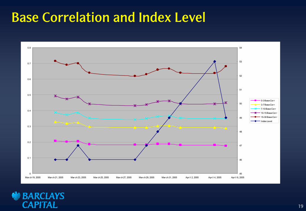
Base Correlation and Index Level

0

0.1

0.2

0.3

0.4

0.5

0.6

0.7

0.8

Mar ch 19, 2005 Mar ch 21, 2005 Mar ch 23, 2005 Mar ch 25, 2005 Mar ch 27, 2005 Mar ch 29, 2005 Mar ch 31, 2005 Apr i l 2, 2005 Apr i l 4, 2005 Apr i l 6, 2005

45

46

47

48

49

50

51

52

53

54

0-3 Base Cor r

3-7 Base Cor r

7-10 Base Cor r

10-15 Base Cor r

15-30 Base Cor r

Index Level

20

Mixture of Copula Functions

� Basic Idea: Correlation is small in good times and large in bad times

� One solution is to make correlation random

� Using copula function we know that the mixture of copula function is still a copula function

)()|()( ρρ

ρ

dVuCUC =

21

Mixture Copula Function: Discrete Case

=

=

=

⋅

m

jj

m

jjmjj uuuC

1

121

,1

;,,,

α

ρα L

22

Gaussian Mixture

� We have three Gaussian copula functions and each with one constant correlation parameter rho

� We also have two independent mixing parameters alpha1 and alpha 2. alpha 3 = 1 – alpha 1 – alpha 2

� We can use this approach to calibrate to the index market with 5 frequently traded tranches

� The calibration is relatively stable. We obtain three correlation parameters around 0%, 25% and 90% and the mixing parameters around 60%, 20% and 20%.

23

Implied Loss Distribution

An equity tranche with tranche size K can be valued as follows:

( )

( )[ ]

( ) )()(

Pr)()(

)()(

2

2

0

KfK

KLE

KLKSKKLE

dxxSKLE

P

P

P

LT

PLT

K

LT

−=∂

∂

>==∂

∂

= ∫

Using market index tranche spreads and base correlation we can obtain the implied loss distribution of CDS index portfolio.

24

Tranche Loss as an Option on the Total Portfolio Loss

Tranche Loss v.s. Total Loss

0

5

10

15

20

25

30

- 10.00 20.00 30.00 40.00

Total Loss

Tran

che

Loss Super Senior

SeniorMezzanineMezzanine SubordEquity

25

Loss Distribution ComparisonsCDX Loss Distribution: Implied, GM, and 15% Flat Gaussian

0%

10%

20%

30%

40%

50%

60%

70%

80%

90%

100%

0.00% 5.00% 10.00% 15.00% 20.00% 25.00% 30.00% 35.00%

strike

Prob

(L >

K)

Market

Gaussian Mixture

Flat 15%

26

Comparison of Leverage Ratios

Comparision of CDX Leverage Ratio

0

2

4

6

8

10

12

14

1 2 3 4 5

Tranches

Leve

rage

Rat

io

Gaussian MixtureGaussian

27

Pricing CDO^2-Type Transactions

� Calculate implied loss distribution

� Obtain model implied loss distribution

� Create a mapping between the market implied loss distribution and model implied loss distribution

� Using this mapping to price all CDOs and CDO^2

� Create a balance between matching to market and also using an economic plausible model

28

Pricing CDO^2-Type Transactions

� Calculate implied loss distribution for each baby portfolio

� Create a mapping between the market implied loss distribution and model implied loss distribution

� Using this mapping to price all CDOs and CDO^2

� Create a balance between matching to market and also using an economic plausible model

29

Loss Distribution Transformation� Transformation (or mapping) function from model implied loss distribution to market implied loss distribution on a cumulativeprobability to a cumulative probability basis. Specifically, let

�This transformation preserves CDO prices.

�This transformation can be applied to multivariate cases

)()(

))(Pr()())(Pr()(

1 LPPLTranform

KtLKPKtLKP

Modelimp

ModelModel

MarketMarket

o−

=

>=

>=

)],0([))((Pr

))((Pr)],0([

0

0 mod

KLEdwwtL

duutLKLE

Ttimp

K

imp

K

elTt

∫

∫=>=

>=

30

Some Theoretical Background on Loss Distribution transformation� We are using this mapping from index to bespoke portfolio transactions: normalized strike based on expected loss, loss ratio and loss distribution percentile to percentile mapping

� In the incomplete market, “risk neutralizing” the statistical distributions from historical data. Madan and Unal (2004)

� Esscher transform or Exponential tilting: Buhlmann (1980) for Pareto optimal equilibrium price, and Gerber and Shiu (1996) for option pricing

� General form: Wang transform (2000)

x

x

XX eEexfxf

λ

λ

⋅=

∗ )()(

λ−ΦΦ=

=

−

∗

))((

)()(1 xF

xFgxF

X

XX

31

CDO^2 Pricing 5-Year

CDO^2 Pricing 5 year

SuperSenior

40-50% 30-40% 20-30% 10-20% Equity

Tranche

Spre

ad in

bas

is p

oint

s

M odel

M ark-It Consensus

M ark-It Consensus+StdDev

M ark-It Consensus-StdDev

32

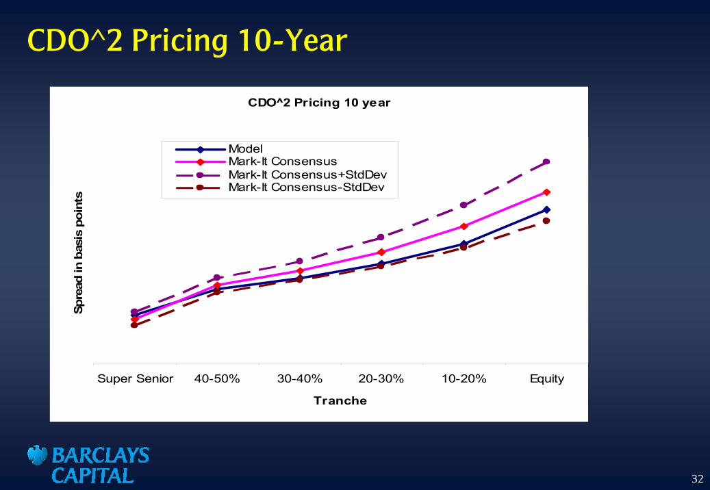
CDO^2 Pricing 10-Year

CDO^2 Pricing 10 year

Super Senior 40-50% 30-40% 20-30% 10-20% Equity

Tranche

Spre

ad in

bas

is p

oint

s

ModelMark-It ConsensusMark-It Consensus+StdDevMark-It Consensus-StdDev

33

Term Structure of Base Correlation

34.43%57.34%40.19%35.96%22.0%

19.19%36.47%28.71%24.72%12.0%

13.68%28.73%23.81%22.93%9.0%

5.81%18.75%18.16%18.95%6.0%

2.72%6.00%8.94%11.82%3.0%

20-Dec-1520-Dec-1220-Dec-1020-Dec-08

Calibrated Base Correlation Term Structure(ITraxx, Feb 10, 2006)Strike

34

Spot Skew and Term Structure Skew (Rainbow)

50.63%56.27%58.69%30.00%53.20%57.42%58.69%30.00%

25.81%32.15%37.98%15.00%27.51%33.06%37.98%15.00%

16.11%22.13%28.59%10.00%17.47%22.88%28.59%10.00%

7.87%14.53%21.15%7.00%9.13%15.16%21.15%7.00%

3.27%3.93%8.44%3.00%4.48%4.51%8.44%3.00%

10 Y7 Y5 YStrike10 Y7 Y5 YStrike

CDX 5 Correlation Skew Term Structure CDX 5 Spot Correlation Skews

35

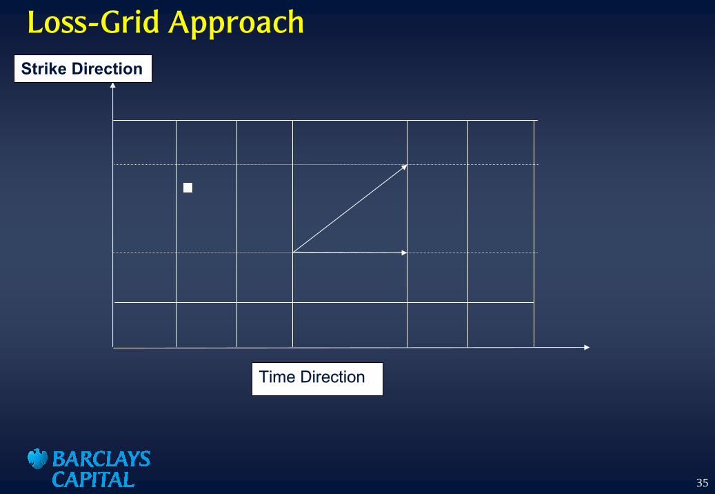
Loss-Grid Approach

Time Direction

Strike Direction

36

Dynamic Models and Some Other Approaches

� To model total portfolio loss only

� Using either short rate type model for instantaneous loss ratio or forward rate model for forward loss ratio

� Functional form, senior tranche, calibration issues

� Sensitivities, going from index to bespoke

� Ultimate Model: replication Model?

� Risk Transformation Approach

37

DisclaimerThis presentation has been prepared by Barclays Capital - the investment banking division of Barclays Bank PLC and its affiliates worldwide (‘Barclays Capital’). This publication is provided to you for information purposes, any pricing in this report is indicative and is not intended as an offer or solicitation for the purchase or sale of any financial instrument. The information contained herein has been obtained from sources believed to be reliable but Barclays Capital does not represent or warrant that it is accurate and complete. The views reflected herein are those of Barclays Capital and are subject to change without notice. Barclays Capital and its respective officers, directors, partners and employees, including persons involved in the preparation or issuance of this document, may from time to time act as manager, co-manager or underwriter of a public offering or otherwise deal in, hold or act as market-makers or advisors, brokers or commercial and/or investment bankers in relation to the securities or related derivatives which are the subject of this report.

Neither Barclays Capital, nor any officer or employee thereof accepts any liability whatsoever for any direct or consequential loss arising from any use of this publication or its contents. Any securities recommendations made herein may not be suitable for all investors. Past performance is no guarantee of future returns. Any modeling or backtesting data contained in this document is not intended to be a statement as to future performance.

Investors should seek their own advice as to the suitability of any investments described herein for their own financial or tax circumstances.

This communication is being made available in the UK and Europe to persons who are investment professionals as that term is defined in Article 19 of the Financial Services and Markets Act 2000 (Financial Promotion Order) 2001. It is directed at persons who have professional experience in matters relating to investments. The investments to which is relates are available only to such persons and will be entered into only with such persons.

Barclays Capital - the investment banking division of Barclays Bank PLC, authorised and regulated by the Financial Services Authority (‘FSA’) and member of the London Stock Exchange.

Copyright in this report is owned by Barclays Capital (© Barclays Bank PLC, 2004) - no part of this report may be reproduced in any manner without the prior written permission of Barclays Capital. Barclays Bank PLC is registered in England No. 1026167. Registered office 54 Lombard Street, London EC3P 3AH.