some like it smooth, and some like it roughweb-docs.stern.nyu.edu/salomon/docs/bollerslev.pdf ·...

Some Like it Smooth, and Some Like it Rough:Untangling Continuous and Jump Components in Measuring,

Modeling, and Forecasting Asset Return Volatility*

Torben G. Andersena, Tim Bollerslevb and Francis X. Dieboldc

First Draft: September 2003This Version: March 2004

Abstract: A rapidly growing literature has documented important improvements in volatilitymeasurement and forecasting performance through the use of realized volatilities constructed from high-frequency returns coupled with relatively simple reduced-form time series modeling procedures. Building on recent theoretical results from Barndorff-Nielsen and Shephard (2003b, 2004a) for related bi-power variation measures involving the sum of high-frequency absolute returns, the present paperprovides a practical framework for non-parametrically measuring the jump component in realizedvolatility measurements. Exploiting these ideas for a decade of high-frequency five-minute returns forthe DM/$ exchange rate, the S&P500 market index, and the 30-year U.S. Treasury bond yield, we findthe jump component of the price process to be distinctly less persistent than the continuous sample pathcomponent. Explicitly including the jump measure as an additional explanatory variable in an easy-to-implement reduced form model for realized volatility results in highly significant jump coefficientestimates at the daily, weekly and quarterly forecast horizons. As such, our results hold promise forimproved financial asset allocation, risk management, and derivatives pricing, by separate modeling,forecasting and pricing of the continuous and jump components of total return variability.

Keywords: Continuous-time methods; jumps; quadratic variation; realized volatility; bi-power variation;high-frequency data; volatility forecasting; HAR-RV model.

JEL Codes: C1, G1

Correspondence: Send all correspondence to Bollerslev.

_________________* This research was supported by the National Science Foundation, the Guggenheim Foundation, and the Wharton FinancialInstitutions Center. We are grateful to Olsen and Associates for generously supplying their intraday exchange rate data. We wouldalso like to thank Neil Shephard and George Tauchen for many insightful discussions and comments, as well as seminar participantsat the September 2003 NBER/NSF Time Series Conference at the University of Chicago, the November 2003 Realized VolatilityConference in Montreal, the December 2003 Conference on Analysis of High-Frequency Financial Data and Market Microstructureat Academia Sineca, Taipei, Taiwan, as well as the Courant Institute at New York University, Baruch College, Princeton, andUppsala University.

a Department of Finance, Kellogg School of Management, Northwestern University, Evanston, IL 60208, and NBER,phone: 847-467-1285, e-mail: [email protected]

b Department of Economics, Duke University, Durham, NC 27708, and NBER,phone: 919-660-1846, e-mail: [email protected]

c Department of Economics, University of Pennsylvania, Philadelphia, PA 19104, and NBER,phone: 215-898-1507, e-mail: [email protected]

Copyright © 2004 T.G. Andersen, T. Bollerslev and F.X. Diebold

1 Earlier influential work on homoskedastic jump-diffusions include Ball and Torous (1983) and Merton (1976), whileJorion (1988) and Vlaar and Palm (1993) have previously incorporated jumps in the estimation of discrete-time ARCH and GARCHmodels; see also the discussion in Das (2002).

1. Introduction

Volatility is central to asset pricing, asset allocation and risk management. In contrast to the

estimation of expected returns, which generally requires long time spans of data, the results in Merton

(1980) and Nelson (1992) suggest that volatility may be estimated arbitrarily well through the use of

sufficiently finely sampled high-frequency returns over any fixed time interval. However, the assumption

of a continuous sample path diffusion underlying these theoretical results is invariably violated in practice

at the highest intradaily sampling frequencies. Thus, despite the increased availability of high-frequency

data for a host of different financial instruments, practical complications have hampered the

implementation of direct high-frequency volatility modeling and filtering procedures (see, e.g., the

discussion in Aït-Sahalia, Mykland and Zhang, 2003; Andersen, Bollerslev and Diebold, 2003; Bai,

Russell, and Tiao, 2001; Bandi and Russell 2003a,b; Engle and Russell, 2003).

In response to this situation, Andersen and Bollerslev (1998), Andersen, Bollerslev, Diebold and

Labys (2001) (henceforth ABDL), Barndorff-Nielsen and Shephard (2002a,b), and Meddahi (2002),

among others, have recently advocated the use of so-called realized volatility measures constructed from

the summation of high-frequency intradaily squared returns as a way of conveniently circumventing the

data complications, while retaining (most of) the relevant information in the intraday data for measuring,

modeling and forecasting volatilities over daily and longer horizons. Indeed, the empirical results in

ABDL (2003) suggest that simple reduced form time series models for realized volatility perform as well,

if not better, than the most commonly used GARCH and related stochastic volatility models in terms of

out-of-sample forecasting.

At the same time, other recent studies have pointed to the importance of explicitly allowing for

jumps, or discontinuities, in the estimation of parametric stochastic volatility models as well as in the

pricing of options and other derivatives instruments (e.g., Andersen, Benzoni and Lund, 2002; Bates,

2000; Chan and Maheu, 2002; Chernov, Gallant, Ghysels, and Tauchen, 2003; Drost, Nijman and

Werker, 1998; Eraker, Johannes and Polson, 2003; Johannes, 2004; Johannes, Kumar and Polson, 1999;

Maheu and McCurdy, 2004; Khalaf, Saphores and Bilodeau, 2003; and Pan, 2002). In particular, it

appears that the conditional variance of many assets is best described by a combination of a smooth and

very slowly mean-reverting continuous sample path process, along with a much less persistent jump

component.1

Set against this backdrop, the present paper seeks to further advance the reduced-form volatility

forecasting procedures advocated in ABDL (2003) through the development of a practical non-parametric

2 Note that this approach is distinctly different from that of Aït-Sahalia (2002), who relies on estimates of the transitiondensity function for identifying jumps.

- 2 -

procedure for separately measuring the continuous sample path variation and the discontinuous jump part

of the quadratic variation process. Our approach builds directly on the new theoretical results in

Barndorff-Nielsen and Shephard (2003a) involving so-called bi-power variation measures constructed

from the summation of appropriately scaled cross-products of adjacent high-frequency absolute returns.2

Implementing these ideas empirically with more than a decade long sample of five-minute high-frequency

returns for the DM/$ foreign exchange market, the S&P500 market index, and the 30-year U.S. Treasury

yield, we shed new light on the dynamic dependencies and the relative importance of jumps across the

different markets. We also demonstrate important gains in terms of volatility forecast accuracy by

explicitly differentiating the jump component. These gains obtain at daily, weekly, and even monthly

forecast horizons. Our new forecasting model incorporating the jumps builds directly on the reduced

form heterogenous AR model for the realized volatility, or HAR-RV model, due to Müller et al. (1997)

and Corsi (2003), in which the realized volatility is parameterized as a linear function of the lagged

realized volatilities over different horizons.

The plan for the rest of the paper is as follows. The next section outlines the basic bi-power

variation theory of Barndorff-Nielsen and Shephard (2003b, 2004a). Section 3 details the data and

highlights the most important qualitative features of the basic jump measurements for each of the three

markets. Section 4 describes the HAR-RV volatility model and the resulting gains obtained by explicitly

including the jump component as an additional explanatory variable. Section 5 presents a simple

statistical procedure for measuring “significant” jumps, and demonstrates that by including the

“significant” jumps and the corresponding continuous sample path variability measures as separate

explanatory variables in the HAR-RV model further enhances the forecast performance. Section 6

concludes with suggestions for future research.

2. Theoretical Framework

Let p(t) denote the time t logarithmic price of the asset. The continuous-time jump diffusion

processes traditionally used in asset pricing finance are then most conveniently expressed in stochastic

differential equation form as,

dp(t) = :(t) dt + F(t) dW(t) + 6(t) dq(t) , 0#t#T, (1)

where :(t) is a continuous and locally bounded variation process, the stochastic volatility process F(t) is

3 Formally, P[q(s)=0, t-h<s#t] = 1 - I0h8(t-h+s)ds + o(h), P[q(s)=1, t-h<s#t] = I0

h8(t-h+s)ds + o(h), and P[q(s)$2, t-h<s#t] = o(h).

- 3 -

strictly positive and continuous, W(t) denotes a standard Brownian motion, dq(t) is a counting process

with dq(t)=1 corresponding to a jump at time t and dq(t)=0 otherwise with (possibly time-varying) jump

intensity 8(t),3 and 6(t)/p(t)-p(t-) refers to the size of the corresponding jumps. The quadratic variation

(or notional volatility/variance in the terminology of ABD, 2003) for the cumulative return process, r(t) /

p(t) - p(0), is then given by

(2)

Of course, in the absence of jumps, the second term on the right-hand-side disappears, and the quadratic

variation is simply equal to the integrated volatility.

Several recent studies involving the direct estimation of continuous time stochastic volatility

models along the lines of equation (1) (e.g., Andersen, Benzoni and Lund, 2002; Eraker, Johannes and

Polson, 2003; Eraker, 2003; Johannes, 2004; Johannes, Kumar and Polson, 1999) have highlighted the

importance of explicitly incorporating jumps in the price process. The specific parametric model

estimates reported in this literature have also generally found the dynamic dependencies in the jumps to

be much less persistent than the dependencies in the continuous sample path volatility process. However,

instead of relying on these model-driven procedures for separately identifying the two components in

equation (2), we will utilize a new non-parametric and purely data-driven high-frequency approach.

2.1. High-Frequency Data, Bi-Power Variation, and Jumps

Let the discretely sampled )-period returns be denoted by, rt,) / p(t) - p(t-)). For ease of notation we

normalize the daily time interval to unity and label the corresponding discretely sampled daily returns by

a single time subscript, rt+1 / rt+1,1. Also, we define the daily realized volatility by the summation of the

corresponding 1/) high-frequency intradaily squared returns,

(3)

where for notational simplicity and without loss of generality 1/) is assumed to be an integer. Then as

emphasized in the series of recent papers by Andersen and Bollerslev (1998), ABDL (2001), Barndorff-

Nielsen and Shephard (2002a,b) and Comte and Renault (1998), among others, by the theory of quadratic

variation this realized volatility converges uniformly in probability to the increment to the quadratic

4 General asymptotic results for so-called realized power variation measures have recently been established by Barndorff-Nielsen and Shephard (2003a, 2004a); see also Barndorff-Nielsen, Graversen and Shephard (2004) for a survey of related results. Inparticular, it follows that in the presence of jumps and for 0<p<2 and )60,

where :p / 2p/2'(½(p+1))/'(½) denotes to the pth absolute moment of a standard normal random variable. Hence, the impact of thediscontinuous jump process disappears in the limit for the power variation measures with 0<p<2. In contrast, RPVt+1(),p) divergesto infinity for p>2, while RPVt+1(),2) / RVt+1()) converges to the integrated volatility plus the sum of the squared jumps, as inequation (4). Related expressions for the conditional moments of different powers of absolute returns have also been utilized by Aït-Sahalia (2003) in the formulation of a GMM-type estimator for specific parametric homoskedastic jump-diffusion models.

5 We shall concentrate on the simplest case involving the summation of adjacent absolute returns, but the general theorydeveloped in Barndorff-Nielsen and Shephard (2003a, 2004a) pertains to other powers and lag lengths as well.

- 4 -

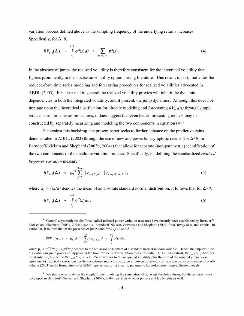
variation process defined above as the sampling frequency of the underlying returns increases.

Specifically, for )60,

(4)

In the absence of jumps the realized volatility is therefore consistent for the integrated volatility that

figures prominently in the stochastic volatility option pricing literature. This result, in part, motivates the

reduced-form time series modeling and forecasting procedures for realized volatilities advocated in

ABDL (2003). It is clear that in general the realized volatility proxies will inherit the dynamic

dependencies in both the integrated volatility, and if present, the jump dynamics. Although this does not

impinge upon the theoretical justification for directly modeling and forecasting RVt+1()) through simple

reduced-form time series procedures, it does suggest that even better forecasting models may be

constructed by separately measuring and modeling the two components in equation (4).4

Set against this backdrop, the present paper seeks to further enhance on the predictive gains

demonstrated in ABDL (2003) through the use of new and powerful asymptotic results (for )60) in

Barndorff-Nielsen and Shephard (2003b, 2004a) that allow for separate (non-parametric) identification of

the two components of the quadratic variation process. Specifically, on defining the standardized realized

bi-power variation measure,5

(5)

where :1 / %(2/B) denotes the mean of an absolute standard normal distribution, it follows that for )60,

(6)

6 A number of recent studies have investigated the practical choice of ) together with different filtering procedures inorder to best mitigate the impact of market microstructure effects in the construction of realized volatility measures (e.g., ABDL,2000; Aït-Sahalia, Mykland and Zhang, 2003; Andreou and Ghysels, 2002; Areal and Taylor, 2002; Bai, Russell and Tiao, 2001;

- 5 -

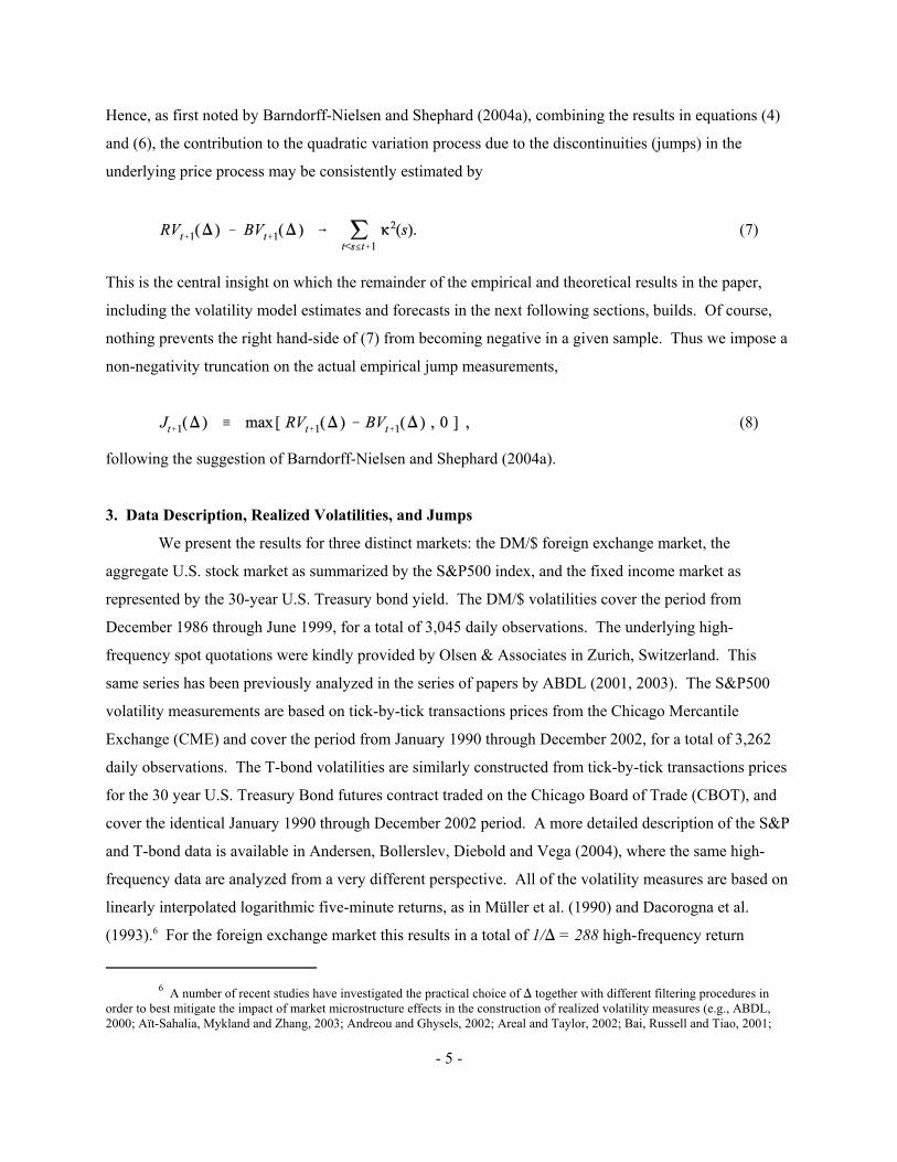
Hence, as first noted by Barndorff-Nielsen and Shephard (2004a), combining the results in equations (4)

and (6), the contribution to the quadratic variation process due to the discontinuities (jumps) in the

underlying price process may be consistently estimated by

(7)

This is the central insight on which the remainder of the empirical and theoretical results in the paper,

including the volatility model estimates and forecasts in the next following sections, builds. Of course,

nothing prevents the right hand-side of (7) from becoming negative in a given sample. Thus we impose a

non-negativity truncation on the actual empirical jump measurements,

(8)

following the suggestion of Barndorff-Nielsen and Shephard (2004a).

3. Data Description, Realized Volatilities, and Jumps

We present the results for three distinct markets: the DM/$ foreign exchange market, the

aggregate U.S. stock market as summarized by the S&P500 index, and the fixed income market as

represented by the 30-year U.S. Treasury bond yield. The DM/$ volatilities cover the period from

December 1986 through June 1999, for a total of 3,045 daily observations. The underlying high-

frequency spot quotations were kindly provided by Olsen & Associates in Zurich, Switzerland. This

same series has been previously analyzed in the series of papers by ABDL (2001, 2003). The S&P500

volatility measurements are based on tick-by-tick transactions prices from the Chicago Mercantile

Exchange (CME) and cover the period from January 1990 through December 2002, for a total of 3,262

daily observations. The T-bond volatilities are similarly constructed from tick-by-tick transactions prices

for the 30 year U.S. Treasury Bond futures contract traded on the Chicago Board of Trade (CBOT), and

cover the identical January 1990 through December 2002 period. A more detailed description of the S&P

and T-bond data is available in Andersen, Bollerslev, Diebold and Vega (2004), where the same high-

frequency data are analyzed from a very different perspective. All of the volatility measures are based on

linearly interpolated logarithmic five-minute returns, as in Müller et al. (1990) and Dacorogna et al.

(1993).6 For the foreign exchange market this results in a total of 1/) = 288 high-frequency return

Bandi and Russell, 2003a,b; Barruci and Reno, 2002; Bollen and Inder, 2002; Corsi, Zumbach, Müller and Dacorogna, 2001; Curciand Corsi, 2003; Hansen and Lunde, 2004; Martens, 2003; Nielsen and Frederiksen, 2004; Oomen, 2002, 2004; Zhang, Aït-Sahaliaand Mykland, 2003). For ease of implementation, we simply follow ABDL (2002, 2001) in the use of unweighted five-minutereturns for each of the three active markets analyzed here.

7 Modeling and forecasting log volatility also has the virtue of automatically imposing non-negativity of fitted andforecasted volatilities.

- 6 -

observations per day, while the two futures contracts are actively traded for 1/) = 97 five-minute

intervals per day. For notational simplicity, we omit the explicit reference to ) in the following, referring

to the five-minute realized volatilities and jumps defined by equations (3) and (8) as RVt and Jt ,

respectively.

The first panels in Figures 1A-C show the resulting three daily realized volatility series in

standard deviation form, or RVt1/2 . Each of the three series clearly exhibits a high degree of own serial

correlation. This is confirmed by the Ljung-Box statistic for up to tenth order serial correlation reported

in Tables 1A-C equal to 5,714, 12,335, and 1,677, respectively. Similar results obtain for the realized

variances and logarithmic transformations reported in the first and third columns in the tables.

Comparing the volatility across the three markets, the S&P500 returns are the most volatile, followed by

the exchange rate returns. Also, consistent with the earlier evidence for the foreign exchange market in

ABDL (2001), and the related findings for individual stocks in Andersen, Bollerslev, Diebold and Ebens

(2002) and for the S&P500 in Deo, Hurvich and Lu (2003) and Martens, van Dijk and Pooter (2003), the

logarithmic standard deviations are generally much closer to being normally distributed than are the raw

realized volatility series. Hence, from a modeling perspective, the logarithmic realized volatilities are

more amenable to the use of standard time series procedures.7

Of course, all of the realized volatility series include the continuous sample path variability as

well as the contribution coming from the jump component. The second panels in Figures 1A-C display

the separate measurements of the jump components (again in standard deviation form) based on the

truncated estimator in equation (8). As is evident from the figures, many of the largest realized

volatilities are directly associated with jumps in the underlying price process. There is also a tendency for

the largest jumps in the DM/$ market to cluster during the earlier 1986-88 part of the sample, while the

size of the jumps for the S&P500 has increased significantly over the most recent 2001-02 two-year

period. Both the size and occurrence of jumps also appear to be more predictable for the S&P500 than

the foreign exchange market. Meanwhile, the jumps in the T-Bond market seem to be much more evenly

distributed throughout the sample.

These visual observations are readily confirmed by the Ljung-Box portmanteau statistics for up to

tenth order serial correlation in the Jt , Jt1/2, and log(Jt +1) series reported in the last three columns in

8 The corresponding ratios for the mean of Jt1/2 relative to the mean RVt

1/2 are 0.193, 0.251, and 0.289 for each of the threemarkets, respectively.

- 7 -

Tables 1A-C. It is noteworthy, however, that although the Ljung-Box statistics for the jumps are

significant at conventional significance levels, the actual values are markedly lower than the

corresponding test statistics for the realized volatility series reported in the first three columns. This

indicates decidedly less predictability in the part of the quadratic variation originating from the

discontinuous sample path part of the process compared to the continuous sample path variation. The

numbers in the table also show that the jumps are relatively least important for the DM/$ market, with the

mean of Jt accounting for 0.072 of the mean of RVt , while the same ratios for the S&P500 and T-bond

markets are 0.146 and 0.125, respectively.8

Motivated by these observations, we now put the idea of separately measuring the jump

component to work in the construction of new and improved realized volatility models and corresponding

forecasts. We follow ABDL (2003) in directly estimating a set of simple reduced-form time series

models for each of the different realized volatility measures in Tables 1A-C; i.e., RVt , RVt1/2, and log(RVt).

Then, in order to assess the added value of separately measuring the jump component in forecasting the

realized volatilities, we simply include the Jt , Jt1/2, and log(Jt

+ 1) jump measurements as additional

explanatory variables in the various forecasting regressions.

4. Reduced-Form Realized Volatility Modeling and Forecasting

A number of empirical studies have argued for the existence of long-memory dependencies in

financial market volatility, and several different parametric ARCH and stochastic volatility formulations

have been proposed in the literature for capturing this phenomenon (e.g., Andersen and Bollerslev, 1997;

Baillie, Bollerslev, and Mikkelsen, 1996; Breidt, Crato and de Lima, 1998; Dacorogna et al., 2001; Ding,

Granger and Engle, 1993; Robinson, 1991). These same empirical observations have also motivated the

estimation of long-memory type ARFIMA models for realized volatility in ABDL (2003), Areal and

Taylor (2002), Deo, Hurvich and Lu (2003), Koopman, Jungbacker and Hol (2004), Martens, van Dijk,

and Pooter (2003), Oomen (2002), Pong, Shackleton, Taylor and Xu (2004), Thomakos and Wang

(2003), among others.

Instead of these relatively complicated estimation procedure, we will here rely on the simple

HAR-RV class of volatility models recently proposed by Corsi (2003). This model is based on a

straightforward extension of the so-called Heterogeneous ARCH, or HARCH, class of models first

introduced by Müller et al. (1997), which parameterizes the conditional variance for a given return

9 Müller et al. (1997) heuristically motivates the HARCH model through the existence of distinct group of traders withdifferent investment horizons.

10 See also the discussion of the use of low-order ARMA models in approximating and forecasting long-memory typebehavior in the conditional mean in Basak, Chan and Palma (2001), Cox (1991), Hsu and Breidt (2003), Man (2003), O’Connell(1971) and Tiao and Tsay (1994), among others, along with the discussion of the related component GARCH model in Engle andLee (1999), the corresponding multi-factor continuous time stochastic volatility model in Gallant, Hsu and Tauchen (1999), and therelated multifractal regime switching models in Calvet and Fisher (2001, 2002).

11 A related set of mixed data sampling, or MIDAS in the terminology of Ghysels, Santa-Clara and Valkanov (2002),regressions for high-frequency foreign exchange rates have recently been estimated by Ghysels, Santa-Clara and Valkanov (2003).

- 8 -

horizon as a function of the lagged squared return over the same and other horizons.9 Although this

model doesn’t formally possess long-memory, the mixing of relatively few volatility components is able

to reproduce a very slow decay that is almost indistinguishable from that of a hyperbolic pattern over

shorter empirically relevant forecast horizons.10

4.1. The HAR-RV-J Model

To sketch the HAR-RV model, define the multi-period realized volatilities by the normalized sum

of the one-period volatilities,

RVt,t+h = h-1[ RVt+1 + RVt+2 + ... + RVt+h ] . (9)

Note that, by definition of the daily volatilities, RVt,t+1 / RVt+1. Also, provided the expectations exist,

E(RVt,t+h)/ E(RVt+1) for all h. Nonetheless, for ease of reference, we will refer to these normalized

volatility measures for h=5 and h=22 as the weekly and monthly volatilities, respectively. The daily

HAR-RV model of Corsi (2003) may then be expressed as

RVt+1 = $0 + $D RVt + $W RVt-5,t + $M RVt-22,t + ,t+1 . (10)

Of course, realized volatilities over other horizons could easily be included as explanatory variables, but

the daily, weekly and monthly measures employed here afford a natural economic interpretation.11

This HAR-RV forecasting model for the one-day volatilities extends straightforwardly to models

for the realized volatilities over other horizons, RVt,t+h. Moreover, given the separate measurements of the

jump components discussed above, these are readily included as additional explanatory variables over and

above the longer-run realized volatility components, resulting in the new HAR-RV-J model,

12 Note, nothing prevents the forecasts for the realized volatilities from an HAR-RV-J model with $J<0 from becomingnegative. We did not find that to be a problem for any of our model estimates, however. Still, a multiplicative error model, alongthe lines of Engle (2002) and Engle and Gallo (2003), could be employed to ensure positivity of the conditional expectations.

- 9 -

RVt,t+h = $0 + $D RVt + $W RVt-5,t + $M RVt-22,t + $J Jt + ,t,t+h . (11)

With single-period observations and longer forecast horizons, or h>1, the error term will generally be

serially correlated up to at least order h-1 due to a standard overlapping data problem. We correct for this

in the standard errors reported below through the use of a Bartlett/Newey-West heteroskedasticity

consistent covariance matrix estimator with 5, 10, and 44 lags for the daily (h=1), weekly (h=5), and

monthly (h=22) estimates, respectively.

Turning to the results reported in the first three columns in Tables 2A-C, the estimates for $D, $W,

and $M confirm the existence of highly persistent dependencies in the volatilities. Interestingly, the

relative importance of the daily volatility component decreases from the daily to the weekly to the

monthly forecasts, whereas the monthly volatility component tends to be relatively more important for the

longer-run monthly forecasts. Importantly, the estimates for the jump component, $J , are systematically

negative across all models and markets, and with few exceptions, overwhelmingly significant.12 Thus,

whereas the realized volatilities are generally highly persistent, the impact of the lagged realized volatility

is significantly reduced on days in which the jump component is active. For instance, for the daily DM/$

realized volatility a unit increase in the daily realized volatility implies an average increase in the

volatility on the following day of 0.430 + 0.196/5 + 0.244/22 = 0.480 for days without any jumps,

whereas for days in which part of the realized volatility comes from the jump component the increase in

the volatility on the following day is reduced by -0.486 times the jump component. In other words, if the

realized volatility is entirely attributable to jumps, it carries no predictive power for the following day’s

realized volatility. Similarly for the other two markets, the combined impact of a jump for forecasting the

next day’s realized volatility equal 0.317 + 0.499/5 + 0.165/22 - 0.436 = -0.012 and 0.069 + 0.316/5 +

0.360/22 - 0.151 = -0.002, respectively. These results are entirely consistent with the parameter estimates

for specific stochastic volatility jump-diffusion models reported in the recent literature, which as

previously noted suggest very little, or no, predictable variation in the jump process.

Comparing the R2 ’s for the HAR-RV-J models to the R2 ’s for the “standard” HAR model

reported in the last row in which the jump component is absent and the realized volatilities on the right-

hand-side but not the left-hand-side of equation (11) are replaced by the corresponding lagged squared

daily, weekly, and monthly returns clearly highlights the added value of high-frequency data in volatility

forecasting. Although the coefficient estimates for the $D, $W, and $M coefficients in the “standard” HAR

13 Note that although the relative magnitude of the R2’s for a given volatility series are directly comparable across the twomodels, as discussed in Andersen, Bollerslev and Meddahi (2003), the measurement errors in the left-hand-side realized volatilitymeasures result in a systematic downward bias in the values of the reported R2’s relative to the predictability of true latent quadraticvariation process.

14 The R2 = 0.431 for the daily HAR-RV-J model for the DM/$ realized volatility series in the fourth column in Table 2Aalso exceeds the comparable in-sample one-day-ahead R2 = 0.355 for the long-memory VAR model reported in ABDL (2003).

- 10 -

models (available upon request) generally are very close to those of the HAR-RV-J models reported in the

tables, the explained variation is systematically much lower.13 Importantly, the gains afforded by the use

of realized volatilities constructed from high-frequency data are not restricted to the daily and weekly

horizons. In fact, the longer-run monthly forecasts result in the largest relative increases in R2 ’s, with

those for the S&P500 and U.S. T-Bonds tripling for the HAR-RV-J models relative to those from the

HAR models based on the coarser daily, weekly and monthly squared returns. These large gains in

forecast accuracy through the use of realized volatilities based on high-frequency data are, of course,

entirely consistent with the earlier empirical evidence in ABDL (2003), Bollerslev and Wright (2001) and

Martens (2002), among others, as well as the related theoretical calculations in Andersen, Bollerslev and

Meddahi (2004).

4.2. Standard Deviation and Logarithmic HAR-RV-J Models

Practical uses of volatility often center on forecasts of standard deviations as opposed to

variances. The second row in each of Tables 2A-C reports the parameter estimates and R2 ’s for the

corresponding HAR-RV-J model cast in the form of standard deviations,

(RVt,t+h)1/2 = $0 + $D RVt1/2 + $W (RVt-5,t)1/2 + $M (RVt-22,t)1/2 + $J Jt

1/2 + ,t,t+h . (12)

The qualitative features and ordering of the different parameter estimates are generally the same as for the

variance formulation in equation (11). In particular, the estimates for $J are systematically negative.

Similarly, the R2 ’s indicate quite dramatic gains for the high-frequency based HAR-RV-J model relative

to the standard HAR model. The more robust volatility measurements provided by the standard

deviations also result in higher R2 ’s than for the variance-based models reported in the first three

columns.14

To further illustrate the predictability afforded by the HAR-RV-J model in equation (12), we plot

in Figures 2A-C the daily, weekly, and monthly realized volatilities (again in standard deviation form)

together with the corresponding forecasts. The close coherence between the different pairs of realizations

15 Of course, if the daily realized volatilities are normally distributed, the weekly and monthly volatilities can not also benormally distributed. However, as argued by Barndorff-Nielsen and Shephard (2002a) and Forsberg and Bollerslev (2002) withinthe context of volatility modeling, the log-normal distribution is closely approximated by the Inverse Gaussian distribution, the laterof which is formally closed under temporal aggregation.

- 11 -

and forecasts is immediately evident across all of the graphs. Visual inspection of the graphs also

confirms that the U.S. T-Bond volatility is the least predictable of the three markets, followed by the

DM/$, and then the S&P500. Nonetheless, the forecasts for the T-Bond volatilities still track the overall

patterns fairly well, especially at the weekly and monthly horizons. The marked increase in equity market

volatility starting in the late 90’s is also directly visible in each of the three panels in Figure 2B.

As noted in Table 1 above, the logarithmic daily realized volatilities are approximately

unconditionally normally distributed for each of the three markets. This empirical regularity motivated

ABDL (2003) to model the logarithmic realized volatilities, in order to invoke the use of standard normal

distribution theory and related mixture models, and this same transformation has subsequently been used

successfully for other markets by Deo, Hurvich and Lu (2003), Koopman, Jungbacker and Hol (2004),

Martens, van Dijk and Pooter (2003), and Oomen (2002) among others.15 Guided by this same idea, we

report in the last three columns of Tables 2A-C the estimates for the HAR-RV-J model cast in logarithmic

form as

log(RVt,t+h) = $0 + $D log(RVt) + $W log(RVt,t-5) + $M log(RVt,t-22)

+ $J log(Jt+1) + ,t,t+h . (13)

The estimates are directly in line with those for the HAR-RV-J models for RVt,t+h and (RVt,t+h)1/2 discussed

previously. In particular, the $D coefficients are generally the largest in the daily models, the $W ’s are the

most important in the weekly models, and the $M ’s in the monthly models. At the same time, the “new”

estimates for the $J coefficients imply that the most significant discontinuities, or jumps, in the price

processes are typically associated with very short-lived bursts in volatility. As previously noted, these

results are generally consistent with the findings in the extant empirical literature on multi-factor jump-

diffusion models. However, the new jump measurements and reduced-form HAR-RV-J models

developed here afford a particularly simple and easy-to-implement modeling procedure for effectively

incorporating these features into more accurate financial market volatility forecasts.

5. Significant Jumps

The empirical results discussed in the previous two sections rely on the simple non-parametric

- 12 -

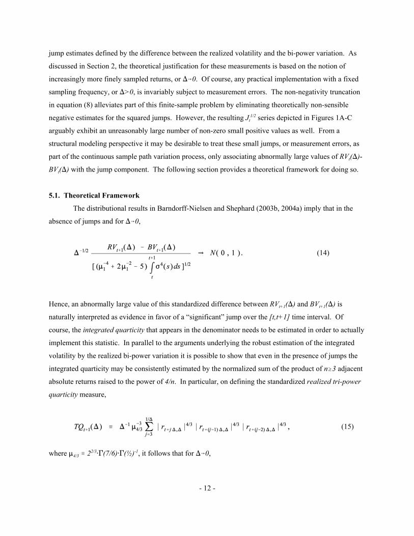
jump estimates defined by the difference between the realized volatility and the bi-power variation. As

discussed in Section 2, the theoretical justification for these measurements is based on the notion of

increasingly more finely sampled returns, or )60. Of course, any practical implementation with a fixed

sampling frequency, or )>0, is invariably subject to measurement errors. The non-negativity truncation

in equation (8) alleviates part of this finite-sample problem by eliminating theoretically non-sensible

negative estimates for the squared jumps. However, the resulting Jt1/2 series depicted in Figures 1A-C

arguably exhibit an unreasonably large number of non-zero small positive values as well. From a

structural modeling perspective it may be desirable to treat these small jumps, or measurement errors, as

part of the continuous sample path variation process, only associating abnormally large values of RVt())-

BVt()) with the jump component. The following section provides a theoretical framework for doing so.

5.1. Theoretical Framework

The distributional results in Barndorff-Nielsen and Shephard (2003b, 2004a) imply that in the

absence of jumps and for )60,

(14)

Hence, an abnormally large value of this standardized difference between RVt+1()) and BVt+1()) is

naturally interpreted as evidence in favor of a “significant” jump over the [t,t+1] time interval. Of

course, the integrated quarticity that appears in the denominator needs to be estimated in order to actually

implement this statistic. In parallel to the arguments underlying the robust estimation of the integrated

volatility by the realized bi-power variation it is possible to show that even in the presence of jumps the

integrated quarticity may be consistently estimated by the normalized sum of the product of n$3 adjacent

absolute returns raised to the power of 4/n. In particular, on defining the standardized realized tri-power

quarticity measure,

(15)

where :4/3 / 22/3@'(7/6)@'(½)-1, it follows that for )60,

16 Similar results were obtained by using the robust realized quad-power quarticity measure advocated in Barndorff-Nielsen and Shephard (2003b, 2004a),

Note however, that the realized quarticity,

used in estimating the integrated quarticity by Barndorff-Nielsen and Shephard (2002a) and Andersen, Bollerslev, and Meddahi(2003) is not consistent in the presence of jumps, in turn resulting in a complete loss of power for the corresponding test statisticobtained by replacing TQt+1()) in equation (17) with RQt+1()).

- 13 -

(16)

Combining the results in equations (14)-(16), the “significant” jumps may therefore be identified by

examining the feasible test statistics,16

(17)

relative to a standard normal distribution.

Recent simulation-based evidence for various continuous time diffusion models in Huang and

Tauchen (2003), suggests that the Wt+1()) statistic defined in (17) tends to over-reject the null hypothesis

of no jumps in the far right tail of the distribution. Hence, following the approach advocated by

Barndorff-Nielsen and Shephard (2004b) and Huang and Tauchen (2003) for improving the finite sample

behavior of the standardized realized volatility distribution, we rely on a log-based version of the test

statistic in (17). Specifically, on applying the delta-rule to the joint bivariate distribution of the realized

volatility and the bi-power variation it follows that the log-transformed test statistic,

(18)

should also be asymptotically normally distributed in the absence of jumps (see also Barndorff-Nielsen

and Shephard, 2003b, 2004a). Importantly, however, the simulation results in Huang and Tauchen (2003)

show that Zt+1()) is generally much better approximated by a normal distribution in the tails than Wt+1()).

17 As noted in personal communication with Neil Shephard, this may alternatively be interpreted as a shrinkage typeestimator for the jump component.

18 This is consistent with the evidence in Andersen, Bollerslev, Diebold and Vega (2003, 2004) among others,documenting discrete intra-daily price jumps in response to a host of macroeconomic news announcements.

- 14 -

Hence, in the following we identify the “significant” jumps by the realizations of Zt+1()) in excess of

some critical value, M" ,

(19)

where I [ @ ] denotes the indicator function.17 Moreover, in order to ensure that the measurements of the

continuous sample path variation and the jump component add up to the realized volatility, the former

component is naturally estimated by the residual relationship,

(20)

Note that for M">0, the definitions in equations (19) and (20) automatically guarantee that both Jt+1," ())

and Ct+1," ()) are positive. Hence by formally specifying "())61 for )60, this approach affords

period-by-period consistent (as )60) estimates of the jump variation and the integrated variance, as well

as the overall quadratic variation process.

In the following, we again omit the explicit reference to the underlying sampling frequency, ),

referring to the “significant” jump and continuous sample path variability measures based on the five-

minute returns as Jt," and Ct," , respectively. Of course, the non-negativity truncation imposed in equation

(8) underlying the empirical jump measurements employed in the preceding two sections simply

corresponds to " = 0.5, or Jt /Jt,0.5 . The next section explores the features of the jump measurements

obtained for other values of " ranging from 0.5 to 0.9999, or M" ranging from 0.0 to 3.719.

5.2. Significant Jump Measurements

The first rows in Tables 3A-C report the proportion of days with significant jumps in each of the

three markets. Although the use of "’s in excess of 0.5 has the intended effect of reducing the number of

days with significant jumps, the procedure still identifies many more jumps than would be expected if the

underlying price process was continuous..18 For instance, employing a cutoff of " =0.999, or M" =3.090,

results in 177, 267, and 385 significant jumps for each of the three markets respectively, all of which far

19 This idea is very briefly pursued in the empirical analysis pertaining to the DM/$ foreign exchange rates reported in thelast section of Barndorff-Nielsen and Shephard (2003b). Similarly, Johannes (2004) readily associates the majority of the largestjumps in his parametric jump-diffusion model estimates for daily interest rates with macroeconomic news announcements.

20 The recent parametric model estimates reported in Chan and Maheu (2002) and McCurdy and Maheu (2004) alsoindicate significant time-varying jump intensities in U.S. equity index returns.

- 15 -

exceed the expected three jumps for a continuous price process (0.001 times 3,045 and 3,262,

respectively). These daily jump proportions are much higher than the jump intensities typically estimated

with specific parametric jump diffusion models applied to daily or coarser frequency returns. This

suggests that many of the jumps identified by the high-frequency based realized volatility measures

employed here may be blurred in the coarser daily or lower frequency returns through an aliasing type

phenomenon. It is also noteworthy that although the proportions of jumps are somewhat sensitive to the

particular choice of ", the sample means of the resulting jump series reported in the second set of rows

depend less on the significance level.

Comparing the jump intensities across the three markets, the T-Bond market generally exhibits

the highest number of jumps, whereas the foreign exchange market has the least. This is consistent with

empirical evidence documenting that the fixed income market is generally the most responsive to

macroeconomic news announcements (see, e.g., Andersen, Bollerslev, Diebold and Vega, 2004). Along

these lines, it would be interesting, but beyond the scope of the present paper, to directly associate the

significant jumps identified here with specific news arrivals, including regularly-scheduled

macroeconomic news releases.19

The Ljung-Box statistics for up to tenth order serial correlation in the Jt," series reported in the

fourth rows indicate highly significant temporal dependencies in the S&P500 jump series for all values of

". Interestingly, the corresponding test statistics for the DM/$ and U.S. T-Bond jump series are not

nearly as large, and generally insignificant for the jumps defined by "’s in excess of 0.950. In contrast,

the tests for serial correlation in the occurrences of jumps, as measured by the Ljung-Box statistics for the

zero-one jump indicator series reported in the fifth set of rows in Tables 3A-C, indicate significant

predictability in the jump intensities for all three markets. These results are at odds with most of the

parametric jump diffusion models hitherto employed in the literature, which typically assume time-

invariant jump intensities.20 Again, it would be interesting, but beyond the scope of the present

paper, to explore more fully the nature of these dependencies in the jump process. Some preliminary

results along these lines suggest that for the S&P500, the larger the jumps the more likely it is for jumps

to occur in the future; i.e., Jt," and Jt+1," >0 are positively correlated. Meanwhile, our estimates for the T-

Bond market suggest an anomalous negative relationship between the strength of the diffusive, or

21 By “optimally” choosing ", it may be possible to further improve upon the empirical results reported below. However, for simplicity and to guard against obvious data snooping biases, we simply restrict "=0.999.

- 16 -

continuous sample path, variability, Ct," , and the future jump intensity, Jt+1," >0. It is worth cautioning,

however, that although statistically significant, these correlations typically explain less than one-percent

of the variability in the zero-one jump indicator series.

The main qualitative features discussed above are underscored by the time series plots for the

significant jump series based on " =0.999 (again in standard deviation form) depicted in the bottom three

panels in Figures 1A-C. The significance tests clearly reduce the number of jumps relative to the Jt1/2

series in the middle set of panels by effectively eliminating most of the smallest jump measures close to

zero. To further illustrate the advantage of this procedure, we next turn to a simple extension of the

HAR-RV-J model discussed in Section 4 in which we incorporate only the significant jumps.

5.3. The HAR-RV-CJ Model

The regression estimates for the HAR-RV-J model in Section 4 show that the inclusion of the

simple consistent daily jump measure as an additional explanatory variable over-and-above the daily

realized volatilities result in highly significant and negative parameter estimations for the jump

coefficient. These results are, of course, entirely consistent with the summary statistics for the jump

measurements discussed above, which indicate markedly less own serial correlation in the significant

jump series in comparison to the realized volatility series. Building on these results, the present section

extends the HAR-RV-J model by explicitly decomposing the realized volatilities that appear as

explanatory variables into the continuous sample path variability and the jump variation utilizing the

separate non-parametric measurements in equations (19) and (20), respectively. In so doing, we rely on "

=0.999, corresponding to the jump series depicted in the bottom panels of Figures 1A-C.21 However, to

facilitate the exposition, we omit the 0.999 subscript on the Jt,0.999 and Ct,0.999 series in what follows.

In particular, on defining the normalized multi-period jump and continuous sample path

variability measures,

Jt,t+h = h-1[ Jt+1 + Jt+2 + ... + Jt+h ] , (21)

and,

Ct,t+h = h-1[ Ct+1 + Ct+2 + ... + Ct+h ] , (22)

respectively, the HAR-RV-CJ model may be expressed as

22 For the two models to be nested the (implicit) choice of " employed in the measurements of Jt,t+h and Ct,t+h should, ofcourse, also be the same across models.

- 17 -

RVt,t+h = $0 + $CD Ct + $CW Ct-5,t + $CM Ct-22,t + (23)

+ $JD Jt + $JW Jt-5,t + $JM Jt-22,t + ,t,t+h .

The model obviously nests the HAR-RV-J model in (11) for $D =$CD +$JD , $W =$CW +$JW , $M =$CM + $JM ,

and $J =$JD , but otherwise allows for more general dynamic dependencies.22

Turning to the empirical estimates in the first three columns in Tables 4A-C, most of the

coefficient estimates for the jump components are insignificant. In other words, the predictability in the

HAR-RV realized volatility regressions are almost exclusively due to the continuous sample path

components. It is also noteworthy that the HAR-RV-CJ models typically result in an increase in the R2 of

about 0.01 in an absolute sense, or about 2-3 percent relatively, compared to the HAR-RV-J models in

Tables 2A-C.

These same qualitative results carry over to the HAR-RV-CJ models cast in standard deviation

form,

(RVt,t+h)1/2 = $0 + $CD Ct1/2 + $CW (Ct-5,t)1/2 + $CM (Ct-22,t)1/2

(24)+ $JD Jt

1/2 + $JW (Jt-5,t)1/2 + $JM (Jt-22,t)1/2 + ,t,t+h ,

and logarithmic form,

log(RVt,t+h) = $0 + $CD log(Ct) + $CW log(Ct-5,t) + $CM log(Ct-22,t)(25)

+ $JD log(Jt +1) + $JW log(Jt-5,t +1) + $JM log(Ct-22,t +1) + ,t,t+h .

The coefficient estimates for the jump components, reported in the last set of columns in Tables 4A-C, are

again insignificant for most of the different markets and horizons. In contrast, the estimates of $CD, $CW

and $CM, which quantify the impact of the continuous sample path variability measures, are generally

highly significant.

All told, these results further underscore the potential benefit from a volatility forecasting

perspective of separately measuring the individual components of the realized volatility. It is possible

that even further improvements may be obtained by a more structured approach (in the sense of

unobserved-components modeling) in which the jump component, Jt , and the continuous sample path

23 The results presented here suggest that the jump component is naturally modeled by a discrete mixture model in whichthe probability of a jump depends non-trivially on past occurrences of jumps, while conditionally on a jump occurring the actual sizeof the jump may depend non-trivially on the time t information set for some but not all markets. Similarly, the empirical evidencediscussed above, along with existing reduced form models for the realized volatility (e.g., Forsberg and Bollerslev, 2002), suggeststhat a Gaussian time series model for log(Ct ) should fit the data for most markets fairly well.

- 18 -

component, Ct , are each modeled separately.23 These individual models for Jt and Ct could then be used

in the construction of separate out-of-sample forecasts for each of the components, as well as combined

forecasts for the total realized volatility process, RVt,t+h = Ct,t+h + Jt,t+h. We leave further work along these

lines for future research.

6. Concluding Remarks

Building on the recent theoretical results for bi-power variation measures in Barndorff-Nielsen

and Shephard (2003b, 2004a), this paper provides a simple practical framework for measuring

“significant” jumps. Applying the idea with more than a decade long sample of high-frequency returns

from the foreign exchange, equity, and fixed income markets, our methods work well empirically.

Consistent with recent parametric estimation results reported in the literature, our measurements of the

jump component are much less persistent (and predictable) than the continuous sample path, or integrated

volatility, component of the quadratic variation process. Using estimates based on underlying high-

frequency data, we identify many more non-zero jumps than do the parametric model estimates based on

daily or coarser data reported in the existing literature. Importantly, our results also indicate significant

improvements in volatility forecasting from separately including the jump measurements as additional

explanatory variables for the future realized volatilities. In fact, when the non-parametric continuous

sample path and jump variability measures are included individually in the same forecasting model, only

the former measures carry any predictive power for the future realized volatilities.

The ideas and empirical results presented here are suggestive of several interesting extensions.

First, recent empirical evidence suggests that jump risk may be priced differently from easier-to-hedge

continuous price variability. Hence, separately modeling and forecasting the continuous sample path, or

integrated volatility, component and the jump component of the quadratic variation process, may result in

more accurate derivatives prices. Second, the high-frequency measures employed here are invariably

subject to various market microstructure biases. Thus, it would be interesting to further investigate the

“optimal” choice of sampling frequency to employ in the construction of the different variation measures.

Along these same lines, it is possible that the procedures for measuring jumps might be improved by off-

setting the absolute returns in the realized bi-power and tri-power variation measures by more than one

period, in turn circumventing some of the market microstructure biases. Third, in addition to the bi-

- 19 -

power variation measures investigated here, the use of more standard power variation measures involving

the sum of properly normalized absolute returns to powers less than two might afford additional gains in

terms of forecast accuracy. Fourth, casual empirical observations suggest that the jumps in the price

processes often occur simultaneously across different markets. Hence, it would be interesting to extend

the present analysis to a multivariate framework incorporating such commonalities through the use of

quadratic covariation and appropriately defined new co-power variation measures. This might also help

in better identifying the most important, or significant, jumps in turn resulting in even larger gains in

forecast accuracy.

References

Aït-Sahalia, Y. (2002), “Telling from Discrete Data Whether the Underlying Continuous-Time Model is aDiffusion,” Journal of Finance, 57, 2075-2121.

Aït-Sahalia, Y. (2003), “Disentangling Volatility from Jumps,” Manuscript, Princeton University.

Aït-Sahalia, Y., P.A. Mykland and L. Zhang (2003), “How Often to Sample a Continuous-Time Process in thePresence of Market Microstructure Noise,” Manuscript, Princeton University.

Andersen, T.G., L. Benzoni and J. Lund (2002), “Estimating Jump-Diffusions for Equity Returns,” Journal ofFinance, 57, 1239-1284.

Andersen, T.G. and T. Bollerslev (1997), “Heterogeneous Information Arrivals and Return VolatilityDynamics: Uncovering the Long-Run in High-Frequency Returns,” Journal of Finance, 52, 975-1005.

Andersen, T.G. and T. Bollerslev (1998), “Answering the Skeptics: Yes, Standard Volatility Models DoProvide Accurate Forecasts,” International Economic Review, 39, 885-905.

Andersen, T.G., T. Bollerslev and F.X. Diebold (2003), “Parametric and Non-Parametric VolatilityMeasurement,” in Handbook of Financial Econometrics (L.P Hansen and Y. Aït-Sahalia, eds.). Elsevier Science, New York, forthcoming.

Andersen, T.G., T. Bollerslev, F.X. Diebold and H. Ebens (2001), “The Distribution of Realized Stock ReturnVolatility,” Journal of Financial Economics, 61, 43-76.

Andersen, T.G., T. Bollerslev, F.X. Diebold and P. Labys (2000), “Great Realizations,” Risk, 13, 105-108.

Andersen, T.G., T. Bollerslev, F.X. Diebold and P. Labys (2001), “The Distribution of Realized ExchangeRate Volatility,” Journal of the American Statistical Association, 96, 42-55.

Andersen, T.G., T. Bollerslev, F.X. Diebold and P. Labys (2003), “Modeling and Forecasting RealizedVolatility,” Econometrica, 71, 579-625.

Andersen, T.G., T. Bollerslev, F.X. Diebold and C. Vega (2003), “Micro Effects of Macro Announcements: Real-Time Price Discovery in Foreign Exchange,” American Economic Review, 93, 38-62.

Andersen, T.G., T. Bollerslev, F.X. Diebold and C. Vega (2004), “Real-Time Price Discovery in Stock, Bondand Foreign Exchange Markets,” Manuscript Northwestern University, Duke University, Universityof Pennsylvania, and University of Rochester.

Andersen, T.G., T. Bollerslev and N. Meddahi (2003), “Correcting the Errors: A Note on Volatility ForecastEvaluation based on High-frequency Data and realized Volatilities,” Manuscript, NorthwesternUniversity, Duke University and University of Montreal.

Andersen, T.G., T. Bollerslev and N. Meddahi (2004), “Analytic Evaluation of Volatility Forecasts,”International Economic Review, forthcoming.

Andreou, E. and E. Ghysels (2002), “Rolling-Sample Volatility Estimators: Some New Theoretical,Simulation, and Empirical Results,” Journal of Business and Economic Statistics, 20, 363-376.

Areal, N.M.P.C. and S.J. Taylor (2002), “The Realized Volatility of FTSE-100 Futures Prices,” Journal ofFutures Market, 22, 627-648.

Bai, X., J.R. Russell and G.C. Tiao (2001), “Beyond Merton’s Utopia: Effects of Non-Normality andDependence on the Precision of Variance Estimates Using High-Frequency Financial Data,”Manuscript, University of Chicago.

Baillie, R.T., T. Bollerslev, and H.O. Mikkelsen (1996), “Fractionally Integrated Generalized AutoregressiveConditional Heteroskedasticity,” Journal of Econometrics, 74, 3-30.

Ball, C.A. and W.N. Torous (1983), “A Simplified Jump Process for Common Stock Returns,” Journal ofFinancial and Quantitative Analysis, 18, 53-65.

Bandi, F.M. and J.R. Russell (2003a), “Microstructure Noise, Realized Volatility and Optimal Sampling,”Manuscript, University of Chicago.

Bandi, F.M. and J.R. Russell (2003b), “Volatility or Microstructure Noise?” Manuscript, University ofChicago.

Barndorff-Nielsen, O.E., S.E. Graversen and N. Shephard (2004), “Power Variation and Stochastic Volatility:A Review and Some New Results,” Journal of Applied Probability, forthcoming.

Barndorff-Nielsen, O.E. and N. Shephard (2002a), “Econometric Analysis of Realised Volatility and its use inEstimating Stochastic Volatility Models,” Journal of the Royal Statistical Society, 64, 253-280.

Barndorff-Nielsen, O.E. and N. Shephard (2002b), “Estimating Quadratic Variation Using RealizedVariance,” Journal of Applied Econometrics, 17, 457-478.

Barndorff-Nielsen, O.E. and N. Shephard (2003a), “Realised Power Variation and Stochastic Volatility,”Bernoulli, 9, 243-265.

Barndorff-Nielsen, O.E. and N. Shephard (2003b), “Econometrics of Testing for Jumps in FinancialEconomics Using Bipower Variation,” Manuscript, Oxford University.

Barndorff-Nielsen, O.E. and N. Shephard (2004a), “Power and Bipower Variation with Stochastic Volatilityand Jumps,” Journal of Financial Econometrics, forthcoming.

Barndorff-Nielsen, O.E. and N. Shephard (2004b), “How Accurate is the Asymptotic Approximation to theDistribution of Realised Volatility,” in Identification and Inference for Econometric Models. AFestschrift in Honour of T.J. Rothenberg (D. Andrews, J. Powell, P.A. Ruud, and J. Stock, eds.). Cambridge, UK: Cambridge University Press.

Basak, G., N.H. Chan, and W. Palma (2001), “The Approximation of Long-Memory Processes by an ARMAModel,” Journal of Forecasting, 20, 367-389.

Bates, D.S. (2000), “Post-`87 Crash fears in the S&P500 Futures Option Market,” Journal of Econometrics,94, 181-238.

Bollen, B. and B. Inder (2002), “Estimating Daily Volatility in Financial Markets Utilizing Intraday Data,”Journal of Empirical Finance, 9, 551-562.

Bollerslev, T. and J.H. Wright (2001), “Volatility Forecasting, High-Frequency Data, and Frequency DomainInference,” Review of Economics and Statistics, 83, 596-602.

Breidt, F.J., N. Crato and P. de Lima (1998), “The Detection and Estimation of Long-Memory in StochasticVolatility,” Journal of Econometrics, 83, 325-348.

Calvet, L. and A. Fisher (2001), “Forecasting Multifractal Volatility,” Journal of Econometrics, 105, 27-58.

Calvet, L. and A. Fisher (2002), “Multifractality in Asset Returns: Theory and Evidence,” Review ofEconomics and Statistics, 84, 381-406.

Chan, W.H. and J.M. Maheu (2002), “Conditional Jump Dynamics in Stock Market Returns,” Journal ofBusiness and Economic Statistics, 20, 377-389.

Chernov, M., A.R. Gallant, E. Ghysels, and G. Tauchen (2003), “Alternative Models for Stock PriceDynamics,” Journal of Econometrics, 116, 225-257.

Comte, F. and E. Renault (1998), “Long Memory in Continuous Time Stochastic Volatility Models,”Mathematical Finance, 8, 291-323.

Corsi, F. (2003), “A Simple Long Memory Model of Realized Volatility,” Manuscript, University of SouthernSwitzerland.

Corsi, F., Zumbach, U.A. Müller and M. Dacorogna (2001), “Consistent High-Precision Volatility from High-frequency Data,” Economic Notes, 30, 183-204.

Cox, D.R. (1991), “Long-Range Dependence, Non-Linearity and Time Irreversibility,” Journal of Time SeriesAnalysis, 12, 329-335.

Curci, G. and F. Corsi (2003), “A Discrete Sine Transform Approach for Realized Volatility Measurement,”Manuscript, University of Pisa.

Dacorogna, M.M., U.A. Müller, R.J. Nagler, R.B. Olsen and O.V. Pictet (1993), “A Geographical Model forthe Daily and Weekly Seasonal Volatility in the Foreign Exchange Market,” Journal of InternationalMoney and Finance, 12, 413-438.

Dacorogna, M.M., R. Gencay, U.A. Müller, O.V. Pictet and R.B. Olsen (2001). An Introduction to High-Frequency Finance. San Diego: Academic Press.

Das, S.R. (2002), “The Surprise Element: Jumps in Interest Rates,” Journal of Econometrics, 106, 27-65.

Deo, R., C. Hurvich, and Y. Lu (2003), “On Forecasting Realized Volatility with High Frequency Returns,”Manuscript, New York University.

Ding, Z., C.W.J. Granger and R.F. Engle (1993), “A Long-Memory Property of Stock Market Returns and aNew Model,” Journal of Empirical Finance, 1, 83-106.

Drost, F.C., T.E. Nijman and B.J.M. Werker (1998), “Estimation and Testing in Models Containing BothJumps and Conditional Heteroskedasticity,” Journal of Business and Economic Statistics, 16, 237-243.

Engle, R.F. (2002), “New Frontiers for ARCH Models,” Journal of Applied Econometrics, 17, 425-446.

Engle, R.F. and G.M. Gallo (2003), “A Multiple Indicators Model for Volatility Using Intra-Daily Data,”Manuscript, New York University.

Engle, R.F. and G.J. Lee (1999), “A Permanent and Transitory Component Model of Stock Return Volatility,”in Cointegration, Causality, and Forecasting: A Festschrift in Honor of Clive W.J. Granger (R.F.Engle and H. White, eds.). Oxford, UK: Oxford University Press.

Eraker, B., M.S. Johannes and N.G. Polson (2003), “the Impact of Jumps in Volatility,” Journal of Finance,58, 1269-1300.

Forsberg, L. and T. Bollerslev (2002), “Bridging the Gap Between the Distribution of Realized (ECU)Volatility and ARCH Modeling (of the Euro): The GARCH-NIG Model,” Journal of AppliedEconometrics, 17, 535-548.

Gallant, A.R., C.T. Hsu and G. Tauchen (1999), “Using Daily Range Data to Calibrate Volatility Diffusionsand Extract the Forward Integrated Variance,” Review of Economics and Statistics, 81, 617-631.

Ghysels, E, P. Santa-Clara and R. Valkanov (2002), “The MIDAS Touch: Mixed Data Sampling RegressionModels,” Manuscript, University of North Carolina and UCLA.

Ghysels, E, P. Santa-Clara and R. Valkanov (2003), “Predicting Volatility: Getting the Most out of ReturnData Sampled at Different Frequencies,” Manuscript, University of North Carolina and UCLA.

Hansen, P.R. and A. Lunde (2004), “Realized Variance and IID Market Microstructure Noise,” BrownUniversity.

Hsu, N.J. and F.J. Breidt (2003), “Bayesian Analysis of Fractionally Integrated ARMA with Additive Noise,”Journal of Forecasting, 22, 491-514.

Huang, X. and G. Tauchen (2003), “The Relative Contribution of Jumps to Total Price Variation,”Manuscript, Duke University.

Johannes, M. (2004), “The Statistical and Economic Role of Jumps in Continuous-Time Interest RateModels,” Journal of Finance, 59, 227-260.

Johannes, M., R. Kumar and N.G. Polson (1999), “State Dependent Jump Models: How do US Equity MarketsJump?” Manuscript, University of Chicago.

Jorion, P. (1988), “On Jump Processes in the Foreign Exchange and Stock Markets,” Review of FinancialStudies, 1, 427-445.

Khalaf, L., J.-D. Saphores and J.-F. Bilodeau (2003), “Simulation-Based Exact Jump Tests in Models withConditional Heteroskedasticity,” Journal of Economic Dynamics and Control, 28, 531-553.

Koopman, S.J., B. Jungbacker and E. Hol (2004), “Forecasting Daily Variability of the S&P100 Stock IndexUsing Historical, Realised and Implied Volatility Measures,” Manuscript, Free UniversityAmsterdam.

Maheu, J.M. and T.H. McCurdy (2004), “News Arrival, Jump Dynamics and Volatility Components forIndividual Stock Returns,” Journal of Finance, forthcoming.

Man, K.S. (2003), “Long Memory Time Series and Short Term Forecasts,” International Journal ofForecasting, 19, 477-491.

Martens, M. (2002), “Measuring and Forecasting S&P500 Index Futures Volatility Using High-FrequencyData,” Journal of Futures Markets, 22, 497-518.

Martens, M., (2003), “Estimating Unbiased and Precise Realized Covariances,” Manuscript, ErasmusUniversity Rotterdam.

Martens, M., D. van Dijk and M. de Pooter (2003), “Modeling and Forecasting &P500 Volatility: Long-Memory, Structural Breaks and Nonlinearity,” Manuscript, Erasmus University Rotterdam.

Meddahi, N. (2002), “A Theoretical Comparison Between Integrated and Realized Volatility,” Journal ofApplied Econometrics, 17, 479-508.

Merton, R.C. (1976), “Option Pricing when Underlying Stock Returns are Discontinuous,” Journal ofFinancial Economics, 3, 125-144.

Merton, R.C. (1980), “On Estimating the Expected Return on the Market: An Exploratory Investigation,”Journal of Financial Economics, 8, 323-361.

Müller, U.A., M.M. Dacorogna, R.B. Olsen, O.V. Puctet, M. Schwarz, and C. Morgenegg (1990), “StatisticalStudy of Foreign Exchange Rates, Empirical Evidence of a Price Change Scaling Law, and IntradayAnalysis,” Journal of Banking and Finance, 14, 1189-1208.

Müller, U.A., M.M. Dacorogna, R.D. Davé, R.B. Olsen, O.V. Puctet, and J. von Weizsäcker (1997),“Volatilities of Different Time Resolutions - Analyzing the Dynamics of Market Components,”Journal of Empirical Finance, 4, 213-239.

Nelson, D.B. (1992), “Filtering and Forecasting with Misspecified ARCH Models I: Getting the RightVariance with the Wrong Model,” Journal of Econometrics, 52, 61-90.

Nielsen, M.Ø. and P.H. Frederiksen (2004), “Finite Sample Accuracy of Integrated Volatility Estimators,”Manuscript, Cornell University.

O’Connell, P.E. (1971), “A Simple Stochastic Modelling of Hurst’s Law,” Proceedings of InternationalSymposium on Mathematical Models in Hydrology, 1, 169-187.

Oomen, R.C.A. (2002), “Modelling Realized Variance when Returns are Serially Correlated,” Manuscript,University of Warwick.

Oomen, R.C.A. (2004), “Properties of Realized Variance for a Pure Jump Process: Calendar Time Samplingversus Business Time Sampling,” Manuscript, University of Warwick.

Pan, J. (2002), “the Jump-Risk Premia Implicit in Options: Evidence from an Integrated Time Series Study,”Journal of Financial Economics, 63, 3-50.

Pong, S., M.B. Shackleton, S.J. Taylor and X. Xu (2004), “Forecasting Currency Volatility: A Comparison ofImplied Volatilities and AR(FI)MA Models,” Journal of Banking and Finance, forthcoming.

Robinson, P.M. (1991), “Testing for Strong Serial Correlation and Dynamic Conditional Heteroskedasticity inMultiple Regressions,” Journal of Econometrics, 47, 67-84.

Tiao, G.C. and R.S. Tsay (1994), “Some Advances in Non-Linear and Adaptive Modeling in Time Series,”Journal of Forecasting, 14, 109-131.

Thomakos, D.D. and T. Wang (2003), “Realized Volatility in the Futures Market,” Journal of EmpiricalFinance, 10, 321-353.

Vlaar, P.J.G. and F.C. Palm (1993), “The Message in Weekly Exchange Rates in the European MonetarySystem: Mean Reversion, Conditional Heteroskedasticity, and Jumps,” Journal of Business andEconomic Statistics, 11, 351-360.

Zhang, L., Y. Aït-Sahalia and P.A. Mykland (2003), “A Tale of Two Time Scales: Determining IntegratedVolatility with Noisy High-Frequency Data,” Manuscript, Princeton University.

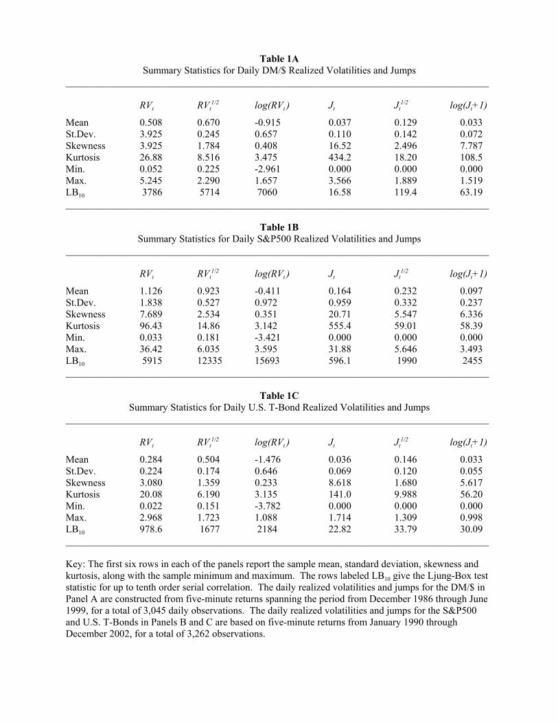
Table 1ASummary Statistics for Daily DM/$ Realized Volatilities and Jumps

____________________________________________________________________________________

RVt RVt1/2 log(RVt ) Jt Jt

1/2 log(Jt+1)

Mean 0.508 0.670 -0.915 0.037 0.129 0.033St.Dev. 3.925 0.245 0.657 0.110 0.142 0.072Skewness 3.925 1.784 0.408 16.52 2.496 7.787Kurtosis 26.88 8.516 3.475 434.2 18.20 108.5Min. 0.052 0.225 -2.961 0.000 0.000 0.000Max. 5.245 2.290 1.657 3.566 1.889 1.519LB10 3786 5714 7060 16.58 119.4 63.19____________________________________________________________________________________

Table 1BSummary Statistics for Daily S&P500 Realized Volatilities and Jumps

____________________________________________________________________________________


1/2 log(Jt+1)

Mean 1.126 0.923 -0.411 0.164 0.232 0.097St.Dev. 1.838 0.527 0.972 0.959 0.332 0.237Skewness 7.689 2.534 0.351 20.71 5.547 6.336Kurtosis 96.43 14.86 3.142 555.4 59.01 58.39Min. 0.033 0.181 -3.421 0.000 0.000 0.000Max. 36.42 6.035 3.595 31.88 5.646 3.493LB10 5915 12335 15693 596.1 1990 2455____________________________________________________________________________________

Table 1CSummary Statistics for Daily U.S. T-Bond Realized Volatilities and Jumps

____________________________________________________________________________________


1/2 log(Jt+1)

Mean 0.284 0.504 -1.476 0.036 0.146 0.033St.Dev. 0.224 0.174 0.646 0.069 0.120 0.055Skewness 3.080 1.359 0.233 8.618 1.680 5.617Kurtosis 20.08 6.190 3.135 141.0 9.988 56.20Min. 0.022 0.151 -3.782 0.000 0.000 0.000Max. 2.968 1.723 1.088 1.714 1.309 0.998LB10 978.6 1677 2184 22.82 33.79 30.09____________________________________________________________________________________

Key: The first six rows in each of the panels report the sample mean, standard deviation, skewness andkurtosis, along with the sample minimum and maximum. The rows labeled LB10 give the Ljung-Box teststatistic for up to tenth order serial correlation. The daily realized volatilities and jumps for the DM/$ inPanel A are constructed from five-minute returns spanning the period from December 1986 through June1999, for a total of 3,045 daily observations. The daily realized volatilities and jumps for the S&P500and U.S. T-Bonds in Panels B and C are based on five-minute returns from January 1990 throughDecember 2002, for a total of 3,262 observations.

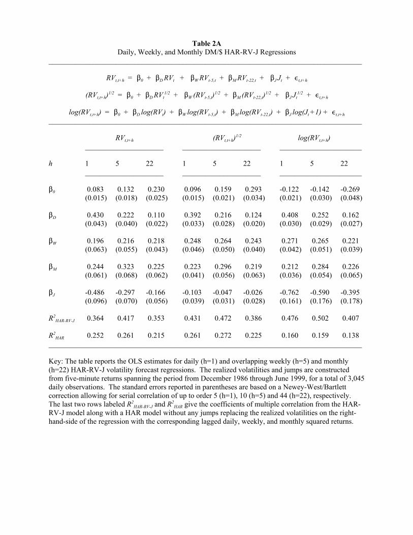
Table 2ADaily, Weekly, and Monthly DM/$ HAR-RV-J Regressions

____________________________________________________________________________________

RVt,t+h = $0 + $D RVt + $W RVt-5,t + $M RVt-22,t + $J Jt + ,t,t+h


1/2 + ,t,t+h

log(RVt,t+h) = $0 + $D log(RVt) + $W log(RVt-5,t) + $M log(RVt-22,t) + $J log(Jt +1) + ,t,t+h____________________________________________________________________________________

RVt,t+h (RVt,t+h)1/2 log(RVt,t+h)_____________________ _____________________ ______________________

h 1 5 22 1 5 22 1 5 22_____________________ _____________________ ______________________

$0 0.083 0.132 0.230 0.096 0.159 0.293 -0.122 -0.142 -0.269(0.015) (0.018) (0.025) (0.015) (0.021) (0.034) (0.021) (0.030) (0.048)

$D 0.430 0.222 0.110 0.392 0.216 0.124 0.408 0.252 0.162(0.043) (0.040) (0.022) (0.033) (0.028) (0.020) (0.030) (0.029) (0.027)

$W 0.196 0.216 0.218 0.248 0.264 0.243 0.271 0.265 0.221(0.063) (0.055) (0.043) (0.046) (0.050) (0.040) (0.042) (0.051) (0.039)

$M 0.244 0.323 0.225 0.223 0.296 0.219 0.212 0.284 0.226(0.061) (0.068) (0.062) (0.041) (0.056) (0.063) (0.036) (0.054) (0.065)

$J -0.486 -0.297 -0.166 -0.103 -0.047 -0.026 -0.762 -0.590 -0.395(0.096) (0.070) (0.056) (0.039) (0.031) (0.028) (0.161) (0.176) (0.178)

R2HAR-RV-J 0.364 0.417 0.353 0.431 0.472 0.386 0.476 0.502 0.407

R2HAR 0.252 0.261 0.215 0.261 0.272 0.225 0.160 0.159 0.138

____________________________________________________________________________________

Key: The table reports the OLS estimates for daily (h=1) and overlapping weekly (h=5) and monthly(h=22) HAR-RV-J volatility forecast regressions. The realized volatilities and jumps are constructedfrom five-minute returns spanning the period from December 1986 through June 1999, for a total of 3,045daily observations. The standard errors reported in parentheses are based on a Newey-West/Bartlettcorrection allowing for serial correlation of up to order 5 (h=1), 10 (h=5) and 44 (h=22), respectively. The last two rows labeled R2

HAR-RV-J and R2HAR give the coefficients of multiple correlation from the HAR-

RV-J model along with a HAR model without any jumps replacing the realized volatilities on the right-hand-side of the regression with the corresponding lagged daily, weekly, and monthly squared returns.

Table 2BDaily, Weekly, and Monthly S&P500 HAR-RV-J Regressions

____________________________________________________________________________________



1/2 + ,t,t+h


RVt,t+h (RVt,t+h)1/2 log(RVt,t+h)_____________________ _____________________ _____________________

h 1 5 22 1 5 22 1 5 22_____________________ _____________________ _____________________

$0 0.093 0.187 0.387 0.063 0.105 0.210 -0.072 -0.003 0.018(0.054) (0.065) (0.072) (0.020) (0.030) (0.038) (0.014) (0.019) (0.036)

$D 0.317 0.213 0.106 0.356 0.253 0.161 0.325 0.220 0.144(0.091) (0.063) (0.039) (0.043) (0.035) (0.029) (0.027) (0.023) (0.023)

$W 0.499 0.441 0.291 0.369 0.404 0.292 0.348 0.368 0.262(0.113) (0.097) (0.091) (0.064) (0.067) (0.069) (0.041) (0.049) (0.048)

$M 0.165 0.215 0.276 0.235 0.266 0.356 0.285 0.339 0.453(0.064) (0.079) (0.086) (0.039) (0.057) (0.068) (0.031) (0.046) (0.053)

$J -0.436 -0.218 -0.070 -0.194 -0.122 -0.047 -0.238 -0.164 -0.083(0.094) (0.079) (0.067) (0.045) (0.039) (0.046) (0.058) (0.063) (0.080)

R2HAR-RV-J 0.412 0.571 0.474 0.599 0.695 0.630 0.678 0.755 0.719

R2HAR 0.249 0.242 0.159 0.320 0.320 0.273 0.196 0.216 0.167

____________________________________________________________________________________

Key: The table reports the OLS estimates for daily (h=1) and overlapping weekly (h=5) and monthly(h=22) HAR-RV-J volatility forecast regressions. The realized volatilities and jumps are constructedfrom five-minute returns spanning the period from January 1990 through December 2002, for a total of3,262 daily observations. The standard errors reported in parentheses are based on a Newey-West/Bartlettcorrection allowing for serial correlation of up to order 5 (h=1), 10 (h=5) and 44 (h=22), respectively. The last two rows labeled R2


RV-J along with a HAR model without jumps replacing the realized volatilities on the right-hand-side ofthe regression with the corresponding lagged daily, weekly, and monthly squared returns.

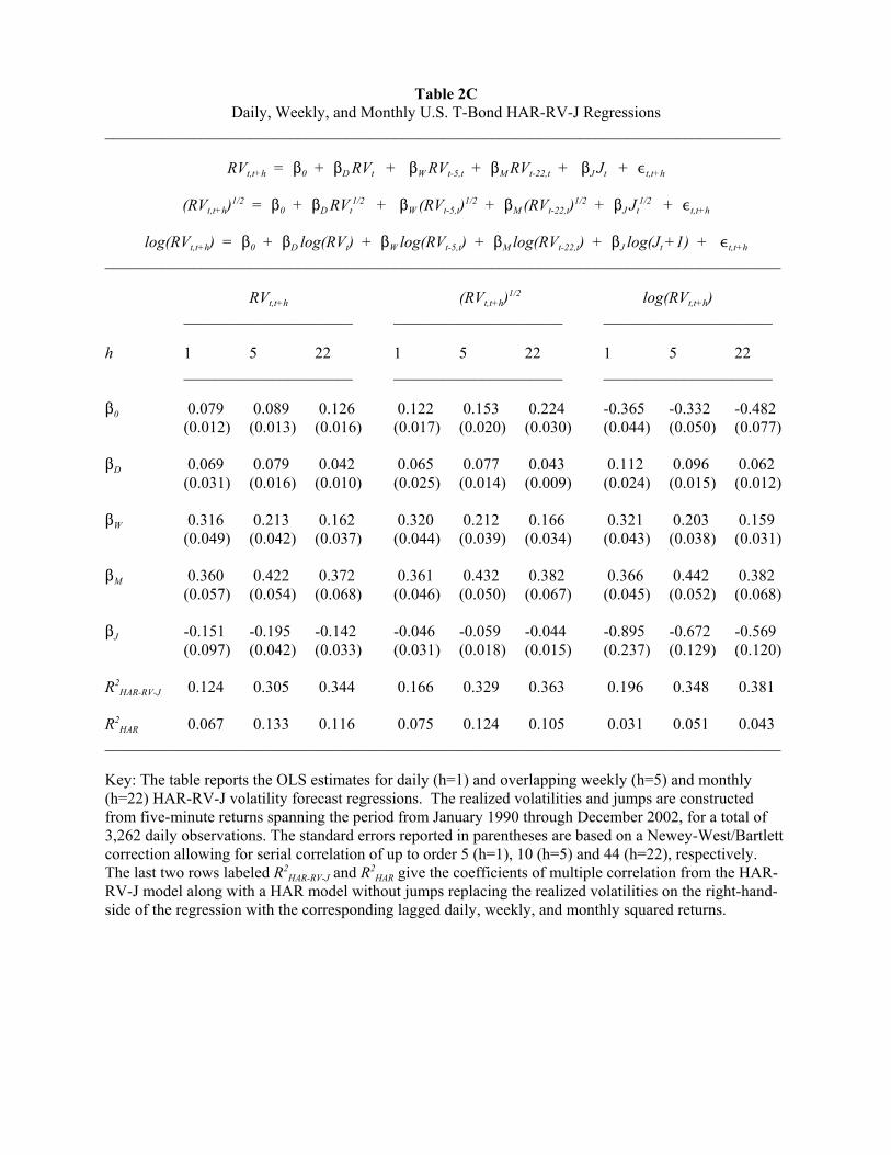
Table 2CDaily, Weekly, and Monthly U.S. T-Bond HAR-RV-J Regressions

____________________________________________________________________________________



1/2 + ,t,t+h


RVt,t+h (RVt,t+h)1/2 log(RVt,t+h)_____________________ _____________________ _____________________

h 1 5 22 1 5 22 1 5 22_____________________ _____________________ _____________________

$0 0.079 0.089 0.126 0.122 0.153 0.224 -0.365 -0.332 -0.482(0.012) (0.013) (0.016) (0.017) (0.020) (0.030) (0.044) (0.050) (0.077)

$D 0.069 0.079 0.042 0.065 0.077 0.043 0.112 0.096 0.062(0.031) (0.016) (0.010) (0.025) (0.014) (0.009) (0.024) (0.015) (0.012)

$W 0.316 0.213 0.162 0.320 0.212 0.166 0.321 0.203 0.159(0.049) (0.042) (0.037) (0.044) (0.039) (0.034) (0.043) (0.038) (0.031)

$M 0.360 0.422 0.372 0.361 0.432 0.382 0.366 0.442 0.382(0.057) (0.054) (0.068) (0.046) (0.050) (0.067) (0.045) (0.052) (0.068)

$J -0.151 -0.195 -0.142 -0.046 -0.059 -0.044 -0.895 -0.672 -0.569(0.097) (0.042) (0.033) (0.031) (0.018) (0.015) (0.237) (0.129) (0.120)

R2HAR-RV-J 0.124 0.305 0.344 0.166 0.329 0.363 0.196 0.348 0.381

R2HAR 0.067 0.133 0.116 0.075 0.124 0.105 0.031 0.051 0.043

____________________________________________________________________________________

Key: The table reports the OLS estimates for daily (h=1) and overlapping weekly (h=5) and monthly(h=22) HAR-RV-J volatility forecast regressions. The realized volatilities and jumps are constructedfrom five-minute returns spanning the period from January 1990 through December 2002, for a total of3,262 daily observations. The standard errors reported in parentheses are based on a Newey-West/Bartlettcorrection allowing for serial correlation of up to order 5 (h=1), 10 (h=5) and 44 (h=22), respectively. The last two rows labeled R2


RV-J model along with a HAR model without jumps replacing the realized volatilities on the right-hand-side of the regression with the corresponding lagged daily, weekly, and monthly squared returns.

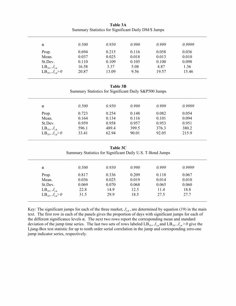
Table 3ASummary Statistics for Significant Daily DM/$ Jumps

____________________________________________________________________________________

" 0.500 0.950 0.990 0.999 0.9999

Prop. 0.694 0.215 0.116 0.058 0.036Mean. 0.037 0.025 0.018 0.013 0.010St.Dev. 0.110 0.109 0.105 0.100 0.098LB10 , Jt," 16.58 3.37 5.08 4.87 1.36LB10 , Jt,">0 20.87 13.09 9.56 19.57 15.46

____________________________________________________________________________________

Table 3BSummary Statistics for Significant Daily S&P500 Jumps

____________________________________________________________________________________

" 0.500 0.950 0.990 0.999 0.9999


____________________________________________________________________________________

Table 3CSummary Statistics for Significant Daily U.S. T-Bond Jumps

____________________________________________________________________________________

" 0.500 0.950 0.990 0.999 0.9999


____________________________________________________________________________________

Key: The significant jumps for each of the three market, Jt," , are determined by equation (19) in the maintext. The first row in each of the panels gives the proportion of days with significant jumps for each ofthe different significance levels ". The next two rows report the corresponding mean and standarddeviation of the jump time series. The last two sets of rows labeled LB10 , Jt," and LB10 , Jt," >0 give theLjung-Box test statistic for up to tenth order serial correlation in the jump and corresponding zero-onejump indicator series, respectively.

Table 4ADaily, Weekly, and Monthly DM/$ HAR-RV-CJ Regressions

____________________________________________________________________________________

RVt,t+h = $0 + $CD Ct + $CW Ct-5,t + $CM Ct-22,t + $JD Jt + $JW Jt-5,t + $JM Jt-22,t + ,t,t+h

(RVt,t+h)1/2 = $0 + $CD Ct1/2 + $CW (Ct-5,t)1/2 + $CM (Ct-22,t)1/2 + $JD Jt

1/2 + $JW (Jt-5,t)1/2 + $JM (Jt-22,t)1/2 + ,t,t+h

log(RVt,t+h) = $0 + $CD log(Ct) + $CW log(Ct-5,t) + $CM log(Ct-22,t) +

$JD log(Jt +1) + $JW log(Jt-5,t +1) + $JM log(Ct-22,t +1) + ,t,t+h____________________________________________________________________________________


h 1 5 22 1 5 22 1 5 22_____________________ _____________________ ______________________

$0 0.087 0.135 0.235 0.097 0.158 0.292 -0.135 -0.149 -0.273(0.015) (0.018) (0.026) (0.015) (0.021) (0.034) (0.019) (0.028) (0.049)

$CD 0.395 0.194 0.093 0.382 0.207 0.119 0.359 0.196 0.125(0.038) (0.035) (0.018) (0.031) (0.027) (0.017) (0.026) (0.020) (0.014)

$CW 0.221 0.246 0.227 0.261 0.295 0.254 0.304 0.333 0.257(0.066) (0.056) (0.044) (0.047) (0.050) (0.042) (0.038) (0.046) (0.040)

$CM 0.230 0.309 0.230 0.207 0.268 0.209 0.210 0.258 0.213(0.062) (0.070) (0.064) (0.041) (0.056) (0.064) (0.034) (0.051) (0.069)

$JD -0.080 -0.037 -0.015 -0.017 -0.001 0.004 -0.146 -0.020 -0.022(0.041) (0.032) (0.019) (0.034) (0.023) (0.012) (0.137) (0.100) (0.064)

$JW -0.311 -0.386 0.092 -0.037 -0.084 0.007 -0.342 -1.036 -0.236(0.171) (0.218) (0.145) (0.046) (0.064) (0.047) (0.332) (0.452) (0.381)

$JM -0.529 -0.512 -0.289 -0.048 0.119 0.062 -0.589 0.248 -0.379(0.524) (0.642) (0.517) (0.062) (0.097) (0.123) (0.599) (1.045) (1.106)

R2HAR-RV-CJ 0.370 0.425 0.356 0.442 0.486 0.395 0.484 0.518 0.414

____________________________________________________________________________________

Key: The table reports the OLS estimates for daily (h=1) and overlapping weekly (h=5) and monthly(h=22) HAR-RV-CJ volatility forecast regressions. All of the realized volatility measures are constructedfrom five-minute returns spanning the period from December 1986 through June 1999, for a total of 3,045daily observations. The weekly and monthly measures are given by the scaled sum of the correspondingdaily measures. The significant daily jump and continuous sample path variability measures are based onequations (19) and (20), respectively, using a critical value of " = 0.999. The standard errors reported inparentheses are based on a Newey-West/Bartlett correction allowing for serial correlation of up to order 5(h=1), 10 (h=5) and 44 (h=22), respectively.

Table 4BDaily, Weekly, and Monthly S&P500 HAR-RV-CJ Regressions

____________________________________________________________________________________



1/2 + $JW (Jt-5,t)1/2 + $JM (Jt-22,t)1/2 + ,t,t+h




h 1 5 22 1 5 22 1 5 22_____________________ _____________________ ______________________

$0 0.118 0.194 0.314 0.060 0.098 0.187 -0.081 0.000 0.039(0.042) (0.055) (0.071) (0.018) (0.028) (0.044) (0.014) (0.020) (0.039)

$CD 0.292 0.180 0.115 0.342 0.231 0.164 0.286 0.196 0.136(0.098) (0.064) (0.035) (0.043) (0.033) (0.023) (0.026) (0.020) (0.020)

$CW 0.500 0.487 0.214 0.370 0.418 0.238 0.374 0.379 0.236(0.144) (0.145) (0.078) (0.067) (0.077) (0.061) (0.042) (0.051) (0.047)

$CM 0.126 0.178 0.442 0.196 0.245 0.422 0.269 0.335 0.488(0.093) (0.115) (0.096) (0.049) (0.070) (0.076) (0.034) (0.050) (0.060)

$JD -0.116 0.018 0.026 -0.007 0.018 0.032 0.021 0.013 0.039(0.077) (0.040) (0.017) (0.052) (0.030) (0.017) (0.070) (0.045) (0.031)

$JW 0.486 0.351 0.524 0.128 0.132 0.166 0.161 0.240 0.334(0.235) (0.151) (0.223) (0.071) (0.062) (0.087) (0.108) (0.108) (0.129)

$JM 0.308 0.309 -0.285 0.103 0.090 0.003 0.123 0.047 -0.145(0.341) (0.422) (0.294) (0.067) (0.093) (0.111) (0.098) (0.135) (0.146)

R2HAR-RV-CJ 0.411 0.571 0.487 0.602 0.695 0.632 0.679 0.758 0.721

____________________________________________________________________________________

Key: The table reports the OLS estimates for daily (h=1) and overlapping weekly (h=5) and monthly(h=22) HAR-RV-CJ volatility forecast regressions. All of the realized volatility measures are constructedfrom five-minute returns spanning the period from January 1990 through December 2002, for a total of3,262 daily observations. The weekly and monthly measures are given by the scaled sum of thecorresponding daily measures. The significant daily jump and continuous sample path variabilitymeasures are based on equations (19) and (20), respectively, using a critical value of " = 0.999. Thestandard errors reported in parentheses are based on a Newey-West/Bartlett correction allowing for serialcorrelation of up to order 5 (h=1), 10 (h=5) and 44 (h=22), respectively.

Table 4CDaily, Weekly, and Monthly U.S. T-Bond HAR-RV-CJ Regressions

____________________________________________________________________________________



1/2 + $JW (Jt-5,t)1/2 + $JM (Jt-22,t)1/2 + ,t,t+h




h 1 5 22 1 5 22 1 5 22_____________________ _____________________ ______________________

$0 0.084 0.093 0.132 0.134 0.163 0.235 -0.334 -0.318 -0.465(0.011) (0.012) (0.016) (0.016) (0.019) (0.029) (0.042) (0.052) (0.078)

$CD 0.036 0.046 0.018 0.043 0.054 0.024 0.061 0.056 0.028(0.027) (0.013) (0.006) (0.023) (0.012) (0.006) (0.022) (0.011) (0.007)

$CW 0.357 0.244 0.183 0.334 0.225 0.173 0.314 0.206 0.162(0.049) (0.043) (0.037) (0.043) (0.039) (0.033) (0.042) (0.039) (0.031)

$CM 0.368 0.439 0.395 0.381 0.447 0.399 0.415 0.465 0.403(0.061) (0.061) (0.070) (0.048) (0.053) (0.068) (0.046) (0.053) (0.067)

$JD 0.060 0.004 -0.006 0.019 0.010 0.005 -0.038 0.038 -0.014(0.100) (0.029) (0.011) (0.036) (0.014) (0.008) (0.309) (0.108) (0.052)

$JW -0.042 -0.058 -0.039 0.035 0.025 0.019 0.165 -0.184 -0.228(0.164) (0.118) (0.093) (0.039) (0.034) (0.028) (0.518) (0.409) (0.343)

$JM -0.371 -0.345 -0.491 -0.174 -0.135 -0.140 -2.893 -1.399 -1.426(0.283) (0.329) (0.326) (0.055) (0.068) (0.080) (0.825) (1.044) (1.184)

R2HAR-RV-CJ 0.130 0.317 0.369 0.177 0.346 0.389 0.206 0.359 0.397

____________________________________________________________________________________

Key: The table reports the OLS estimates for daily (h=1) and overlapping weekly (h=5) and monthly(h=22) HAR-RV-CJ volatility forecast regressions. All of the realized volatility measures are constructedfrom five-minute returns spanning the period from January 1990 through December 2002, for a total of3,262 daily observations. The weekly and monthly measures are given by the scaled sum of thecorresponding daily measures. The significant daily jump and continuous sample path variabilitymeasures are based on equations (19) and (20), respectively, using a critical value of " = 0.999. Thestandard errors reported in parentheses are based on a Newey-West/Bartlett correction allowing for serialcorrelation of up to order 5 (h=1), 10 (h=5) and 44 (h=22), respectively.

0 . 0

0 . 5

1 . 0

1 . 5

2 . 0

2 . 5

0 . 0

0 . 5

1 . 0

1 . 5

2 . 0

2 . 5

0 . 0

0 . 5

1 . 0

1 . 5

2 . 0

2 . 5

Figure 1ADaily DM/$ Realized Volatilities and Jumps

Key: The top panel shows daily realized volatility in standard deviation form, or RVt1/2. The middle

panel shows the estimated jump component, and the bottom panel shows the “significant” jumps using acutoff value of " =0.999. See text for details and sample periods.

0

1

2

3

4

5

6

0

1

2

3

4

5

6

0

1

2

3

4

5

6

Figure 1BDaily S&P500 Realized Volatilities and Jumps



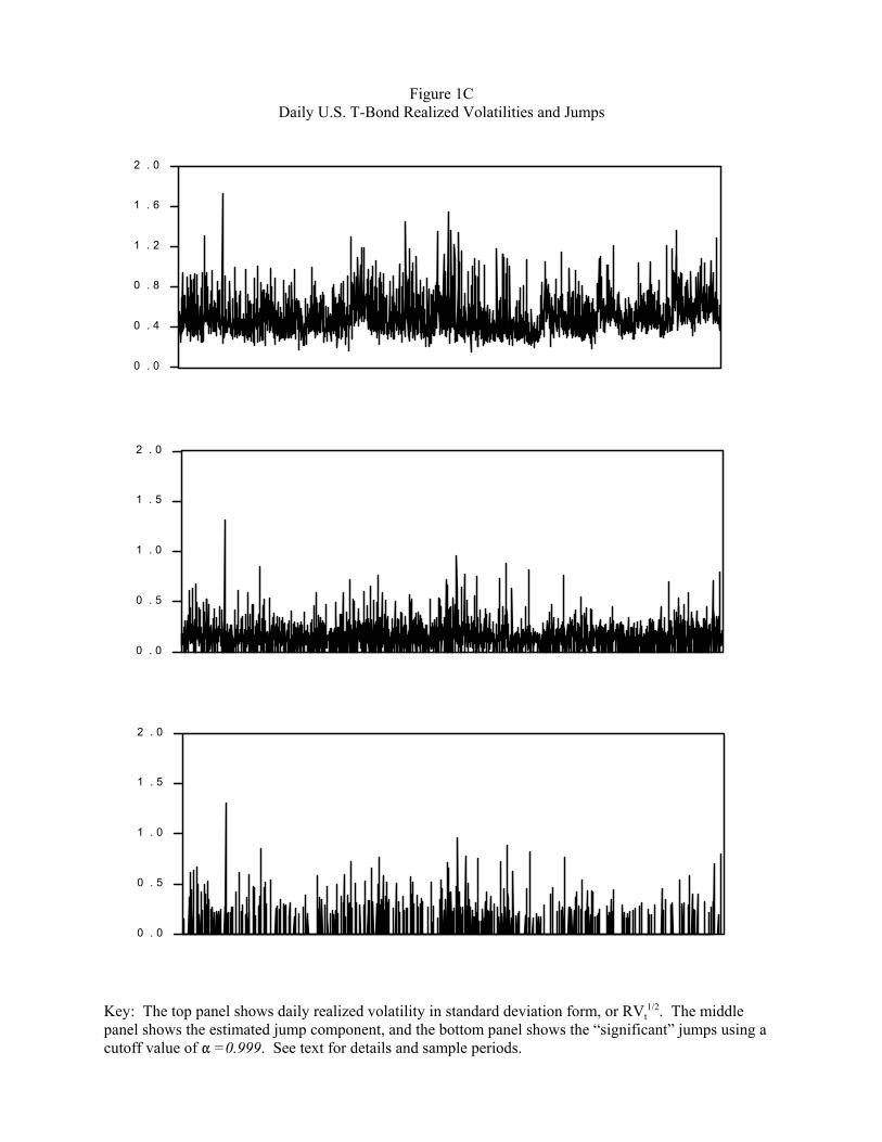
0 . 0

0 . 4

0 . 8

1 . 2

1 . 6

2 . 0

0 . 0

0 . 5

1 . 0

1 . 5

2 . 0

0 . 0

0 . 5

1 . 0

1 . 5

2 . 0

Figure 1CDaily U.S. T-Bond Realized Volatilities and Jumps



0 . 0

0 . 4

0 . 8

1 . 2

1 . 6

0 . 0

0 . 4

0 . 8

1 . 2

1 . 6

0 . 0

0 . 5

1 . 0

1 . 5

2 . 0

0 . 0

0 . 5

1 . 0

1 . 5

2 . 0

0 . 0

0 . 5

1 . 0

1 . 5

2 . 0

2 . 5

0 . 0

0 . 5

1 . 0

1 . 5

2 . 0

2 . 5

Figure 2ADaily, Weekly and Monthly HAR-RV-J DM/$ Realized Volatility Forecasts

Key: The top, middle and bottom panels show daily, weekly and monthly realized volatilities (left scale)and forecasts (right scale). See text for details and sample periods.

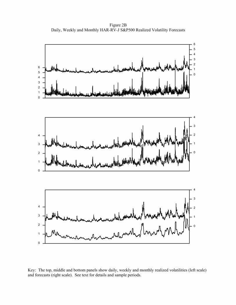
0

1

2

3

4

5

6

0

1

2

3

4

5

6

0

1

2

3

4

0

1

2

3

4

0

1

2

3

4

0

1

2

3

4

Figure 2BDaily, Weekly and Monthly HAR-RV-J S&P500 Realized Volatility Forecasts


0 . 0

0 . 2

0 . 4

0 . 6

0 . 8

1 . 0

0 . 0

0 . 2

0 . 4

0 . 6

0 . 8

1 . 0

0 . 0

0 . 4

0 . 8

1 . 2

0 . 0

0 . 4

0 . 8

1 . 2

0 . 0

0 . 4

0 . 8

1 . 2

1 . 6

2 . 0

0 . 0

0 . 5

1 . 0

1 . 5

2 . 0

Figure 2CDaily, Weekly and Monthly HAR-RV-J T-Bond Realized Volatility Forecasts


some like it smooth, and some like it roughweb-docs.stern.nyu.edu/salomon/docs/bollerslev.pdf ·...

Documents