some logistics some version problems with homework solutions posted to website. all fixed now.some...
TRANSCRIPT

Some LogisticsSome Logistics
• Some version problems with homework solutions Some version problems with homework solutions posted to website. All fixed now.posted to website. All fixed now.
• Cummings lecture (1/31) not recorded. Video and Cummings lecture (1/31) not recorded. Video and slides from 2012 posted. Dr. Cummings would like to slides from 2012 posted. Dr. Cummings would like to strongly encourage you to attend his final lecture on strongly encourage you to attend his final lecture on 3/21.3/21.
• Sample size planning added to 2/21 lecture. Addition of Sample size planning added to 2/21 lecture. Addition of second reading assignment from DCR. Will be changed second reading assignment from DCR. Will be changed on online syllabus.on online syllabus.

Data Analysis Issues in Clinical TrialsData Analysis Issues in Clinical Trials
• Overview of simple data analysis for clinical trialsOverview of simple data analysis for clinical trials
• Data analysis for non-standard study designsData analysis for non-standard study designs– Cross overCross over
– Cluster randomizationCluster randomization
– Factorial designsFactorial designs
• Multiple comparisons in clinical trialsMultiple comparisons in clinical trials
• Special topics in data analysis in RCT’s (today and 2/21 lecture)Special topics in data analysis in RCT’s (today and 2/21 lecture)– Subgroups (Wang, et al, assigned reading)Subgroups (Wang, et al, assigned reading)
– Adjustment for baseline covariablesAdjustment for baseline covariables
– Multiple endpointsMultiple endpoints
• Other issues to be covered later: ITT, non-compliance, etc.Other issues to be covered later: ITT, non-compliance, etc.

Overview of data analysis for clinical trials Overview of data analysis for clinical trials
• Example: 2 treatment groups (active/placebo)Example: 2 treatment groups (active/placebo)
• Goal: compare something in active vs. placeboGoal: compare something in active vs. placebo
• What is appropriate analysis?What is appropriate analysis?
• Analysis depends on type of outcome variableAnalysis depends on type of outcome variable
–Continuous (eg. cholesterol level, BP)Continuous (eg. cholesterol level, BP)
–Binary (y/n) (eg. death yes/no)Binary (y/n) (eg. death yes/no)
–Binary, time to event (eg. time to prostate Binary, time to event (eg. time to prostate cancer)cancer)

Comparison of 2 treatment groups in RCTComparison of 2 treatment groups in RCT
• Depends on type of outcome variableDepends on type of outcome variable–Continuous (t-test or non-parametric)Continuous (t-test or non-parametric)
–Binary (y/n) (chi-squared)Binary (y/n) (chi-squared)
–Binary, time to event (log rank)Binary, time to event (log rank)
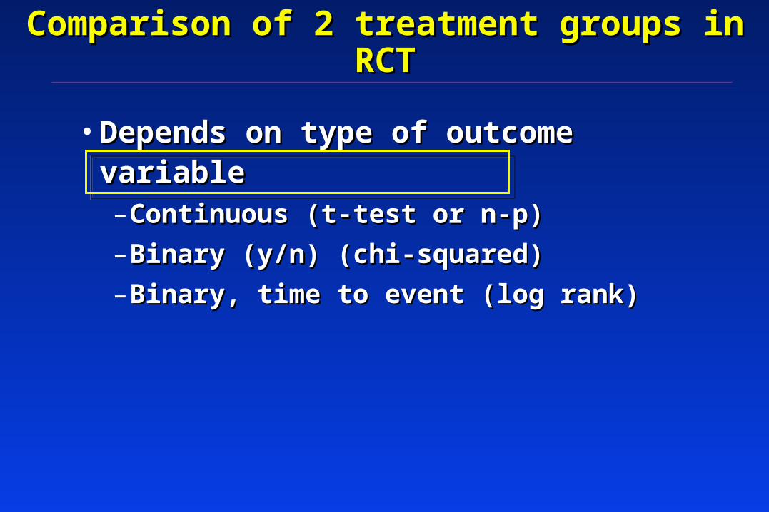
Comparison of 2 treatment groups in RCTComparison of 2 treatment groups in RCT
• Depends on type of outcome variableDepends on type of outcome variable–Continuous (t-test or n-p)Continuous (t-test or n-p)
–Binary (y/n) (chi-squared)Binary (y/n) (chi-squared)
–Binary, time to event (log rank)Binary, time to event (log rank)

Continuous Outcomes: AnalysisContinuous Outcomes: Analysis
• Compare mean in placebo with mean in activeCompare mean in placebo with mean in active– e.g., effect of statins on lipids, b-blocker on BPe.g., effect of statins on lipids, b-blocker on BP
• Usually compare mean change across two groupsUsually compare mean change across two groups– Increased powerIncreased power
– Valid to compare “after” onlyValid to compare “after” only
• Other examples:Other examples:– Change in menopausal symptoms scoreChange in menopausal symptoms score
– Change in weight (RCT’s of diets)Change in weight (RCT’s of diets)
– Change in bone densityChange in bone density

• 2 continuous endpoints2 continuous endpoints– Change in bone density (%) Change in bone density (%)
– Markers of bone remodelingMarkers of bone remodeling
• P-M women, 55-85 years P-M women, 55-85 years
• Randomize (1 year, double blind) to:Randomize (1 year, double blind) to:– PTH alone (119)PTH alone (119)
– PTH + Alendronate (59)PTH + Alendronate (59)
– (Others) (Others)
PTH and Alendronate (PaTH)*:PTH and Alendronate (PaTH)*:Example of continuous endpointExample of continuous endpoint
* Black, et. al. NEJM (9/23/03)* Black, et. al. NEJM (9/23/03)

Changes in Trabecular Spine Bone Changes in Trabecular Spine Bone Density (%) in PaTHDensity (%) in PaTH
Spine BMDSpine BMD00
1010
2020
3030
4040
PTHPTH PTH/ALNPTH/ALN
Me
an
Ch
an
ge
(%)
Me
an
Ch
an
ge
(%)
**** **** p<.01 by t-test p<.01 by t-test
* Black, et. al. NEJM (9/23/03)* Black, et. al. NEJM (9/23/03)

Little Known Facts about Boring Tests:Little Known Facts about Boring Tests:Who is “Student”?Who is “Student”?
• Student’s t-test
• Developed by W.S. Gossett ("Student”) [1876-1937]
• Developed as statistical method to solve problems stemming from his employment in...??
• A brewery
• Quiz 1: Which brewery did “Student” work for?
– Ans: Guinness

When is a T-test Valid?When is a T-test Valid?
• If the outcome variable is normally distributed, use a t-If the outcome variable is normally distributed, use a t-test. If the outcome is not normal, use a nonparametric test. If the outcome is not normal, use a nonparametric test such as a Wilcoxin test.test such as a Wilcoxin test.
• True or False?True or False?
Ans: FalseAns: False
T-test is valid even T-test is valid even when variables are when variables are somewhat non-normalsomewhat non-normal

When is When is tt-test Valid-test Valid
• tt-test requires that sample means (not individuals) are normally -test requires that sample means (not individuals) are normally distributed.distributed.
• What does CLT stand for?What does CLT stand for?
• Central Limit TheoremCentral Limit Theorem
– (The mean from any variable becomes normally distributed as (The mean from any variable becomes normally distributed as n becomes larger (goes to infinity) )n becomes larger (goes to infinity) )
• Practical implication:Practical implication: tt-test-test almost always valid for continuous almost always valid for continuous
data as long as n is large enough or variable not too weird.data as long as n is large enough or variable not too weird.

Badly behaved continuous outcomesBadly behaved continuous outcomes(eg. days of back pain)(eg. days of back pain)
• Use Use tt-test usually-test usually
• If radically non-normal, use If radically non-normal, use non-parametric analoguenon-parametric analogue
– ExamplesExamples– 1. cigarettes per day1. cigarettes per day– 2. Days of back pain2. Days of back pain

Another badly behaved variable:Another badly behaved variable:% Change in Markers of Bone Turnover with PTH therapy in % Change in Markers of Bone Turnover with PTH therapy in
PaTH*PaTH*F
requ
ency
(%
) 60
40
20
0
80
1 Year Change (%)
0 90 180 270 360-90 450 540 630
For strong departures For strong departures from normality, use non-from normality, use non-parametric techniquesparametric techniques
Black, et. al. NEJM 2002Black, et. al. NEJM 2002Black, et. al. NEJM 2002Black, et. al. NEJM 2002

% Changes in Markers of Bone Turnover% Changes in Markers of Bone Turnover(Use medians and interquartile range, Wilcoxin test)(Use medians and interquartile range, Wilcoxin test)
Me
dia
n C
ha
ng
e (
%)
Me
dia
n C
ha
ng
e (
%)
-100-100
00
100100
200200
300300
400400
00 33 66 99 1212MonthMonth
PTH PTH PTH/ALN PTH/ALN
Formation (P1NP)Formation (P1NP) 7575thth percentile: +400% percentile: +400%
(Increases as high as (Increases as high as 800%)800%)
2525thth percentile (25%) percentile (25%)
Median (150%)Median (150%)

Comparison of 2 treatment groups in RCTComparison of 2 treatment groups in RCT
• Depends on type of outcome variableDepends on type of outcome variable–Continuous (t-test)Continuous (t-test)
–Binary (y/n) (chi-squared)Binary (y/n) (chi-squared)
–Binary, time to event (log rank)Binary, time to event (log rank)
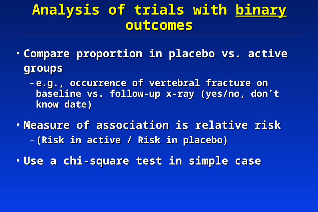
Analysis of trials with Analysis of trials with binarybinary outcomes outcomes
• Compare proportion in placebo vs. active groupsCompare proportion in placebo vs. active groups– e.g., occurrence of vertebral fracture on baseline vs. e.g., occurrence of vertebral fracture on baseline vs.
follow-up x-ray (yes/no, don’t know date)follow-up x-ray (yes/no, don’t know date)
• Measure of association is relative riskMeasure of association is relative risk– (Risk in active / Risk in placebo)(Risk in active / Risk in placebo)
• Use a chi-square test in simple caseUse a chi-square test in simple case

3 Years of Raloxifene in MORE: 3 Years of Raloxifene in MORE: Effect on Vertebral Fracture*Effect on Vertebral Fracture*
Relative Risk (RR)=0.65Relative Risk (RR)=0.65(0.53, 0.79)(0.53, 0.79)
P=??P=??%
wit
h f
ract
ure
% w
ith
fra
ctu
re
PBOPBO RLX 60 RLX 60
*Vertebral fractures *Vertebral fractures assessed from x-rays assessed from x-rays at baseline compared at baseline compared to end of trialto end of trial
p<.01p<.01

Comparison of 2 treatment groups in RCTComparison of 2 treatment groups in RCT
• Depends on type of outcome variableDepends on type of outcome variable–Continuous (t-test)Continuous (t-test)
–Binary (y/n) (chi-squared)Binary (y/n) (chi-squared)
–Binary, time to event (log rank)Binary, time to event (log rank)

Analysis of trials with time-to-event outcomesAnalysis of trials with time-to-event outcomes
• Compare survival curves in active vs. placebo Compare survival curves in active vs. placebo groupsgroups
• Measure of association is the Relative Hazard Measure of association is the Relative Hazard (RH) or Hazard Ratio (HR)(RH) or Hazard Ratio (HR)
• Similar to Relative RiskSimilar to Relative Risk
• Use log rank testUse log rank test– Stratified chi-square at each “failure” timeStratified chi-square at each “failure” time
– Equivalent to proportional hazards model with single Equivalent to proportional hazards model with single binary predictor (hazard ratio)binary predictor (hazard ratio)

Survival Curve example: Women’s Health Survival Curve example: Women’s Health Initiative (HRT vs PBO): Coronary Heart Initiative (HRT vs PBO): Coronary Heart
DiseaseDisease
years 1 2 3 4 5 6 7

p < 0.001p < 0.001(log rank test)(log rank test)
Raloxifene and Risk ofRaloxifene and Risk ofBreast Cancer (MORE trial)Breast Cancer (MORE trial)
YearsYears
0.00
0.25
0.50
0.75
1.00
1.25
0 1 2 3 4
% o
f pa
rtic
ipan
ts%
of
part
icip
ants
PlaceboPlacebo3.8 per 1,0003.8 per 1,000
RaloxifeneRaloxifene1.7 per 1,0001.7 per 1,000

WHI: Invasive Breast CancerWHI: Invasive Breast Cancer
years 1 2 3 4 5 6 7
1%
2%
3%

Intro to Data Analysis for Intro to Data Analysis for More Exotic RCT Designs More Exotic RCT Designs
• Cluster randomization designsCluster randomization designs
• Factorial designsFactorial designs
• Repeated measures designRepeated measures design
• Cross-over designsCross-over designs
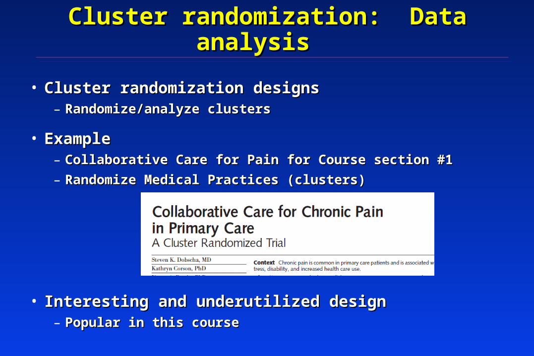
Cluster randomization: Data analysisCluster randomization: Data analysis
• Cluster randomization designsCluster randomization designs– Randomize/analyze clustersRandomize/analyze clusters
• ExampleExample– Collaborative Care for Pain for Course section #1Collaborative Care for Pain for Course section #1
– Randomize Medical Practices (clusters)Randomize Medical Practices (clusters)
• Interesting and underutilized designInteresting and underutilized design– Popular in this coursePopular in this course

Cluster randomization: JAMA studyCluster randomization: JAMA study
•46 clinicians46 clinicians
•401 patients401 patients
•46 clinicians46 clinicians
•401 patients401 patients

Cluster randomization of CliniciansCluster randomization of Clinicians
100 kids100 kids100 kids100 kids~10 patients~10 patients~10 patients~10 patients
~10 patients~10 patients~10 patients~10 patients
~10 patients~10 patients~10 patients~10 patients
~10 patients~10 patients~10 patients~10 patients
~10 patients~10 patients~10 patients~10 patients
~10 patients~10 patients~10 patients~10 patients ~10 patients~10 patients~10 patients~10 patients
~10 patients~10 patients~10 patients~10 patients
46 clinicians, 46 clinicians, 401 patients401 patients

Cluster randomization: AnalysisCluster randomization: Analysis
• Analysis must account for randomization of clusters, not Analysis must account for randomization of clusters, not individualsindividuals
• Most commonly used technique: Generalized Estimating Most commonly used technique: Generalized Estimating Equations (GEE)Equations (GEE)– Type of multiple regression Type of multiple regression
– In Stata and SASIn Stata and SAS
• Effective sample size is between total n and number of Effective sample size is between total n and number of clustersclusters
– Methods (see following 3 slides, not presented in class)Methods (see following 3 slides, not presented in class)

Cluster randomization: Cluster randomization: Steps in sample size calculationSteps in sample size calculation
1. Calculate sample size as if total n1. Calculate sample size as if total n
2. Inflation factor:2. Inflation factor:
= (1 + (CS-1)*RHO)= (1 + (CS-1)*RHO)
Where :Where : CS=cluster sizeCS=cluster size
RHO=Intraclass corr. coef.RHO=Intraclass corr. coef.
CSCS RHORHO InflationInflation
3030 .05.05 x 1.5x 1.5
100100 .05.05 x 6x 6
10001000 .05.05 x 51x 51
eg. if n=100 with eg. if n=100 with no clustersno clusters
150150
600600
51,00051,000

Cluster randomization: Sample sizeCluster randomization: Sample size
How big is intraclass correlation (rho)?How big is intraclass correlation (rho)?
- Degree of similarity within cluster. Corr. Coefficient within - Degree of similarity within cluster. Corr. Coefficient within cluster (0=no relationship to 1)cluster (0=no relationship to 1)
-In Collaborative Pain Study in section, assumed rho=.05 for -In Collaborative Pain Study in section, assumed rho=.05 for sample sizesample size
-Some empiric studies suggest: in range of .01 to .2 for clusters -Some empiric studies suggest: in range of .01 to .2 for clusters like medical practice or communitylike medical practice or community
- Need pilot data--Challenge in planning a cluster randomization - Need pilot data--Challenge in planning a cluster randomization studystudy

Some References for Cluster Randomization Some References for Cluster Randomization DesignsDesigns
– Eldridge, S. M., D. Ashby, et al. (2004). "Lessons for cluster randomized trials in the twenty-first century: a systematic review of trials in primary care." Clin Trials 1(1): 80-90.
– Gulliford, M. C., O. C. Ukoumunne, et al. (1999). "Components of variance and intraclass correlations for the design of community-based surveys and intervention studies: data from the Health Survey for England 1994." Am J Epidemiol 149(9): 876-83.
– Smeeth, L. and E. S. Ng (2002). "Intraclass correlation coefficients for cluster randomized trials in primary care: data from the MRC Trial of the Assessment and Management of Older People in the Community." Control Clin Trials 23(4): 409-21.

Factorial design: Analysis Implications Factorial design: Analysis Implications
• Factorial designsFactorial designs–Seductive but trickySeductive but tricky
–Need to believe and show that no interaction Need to believe and show that no interaction between treatments (statistical test)between treatments (statistical test)
• Examples:Examples:–Vitamin C and E on prostate cancer (Gaziano)Vitamin C and E on prostate cancer (Gaziano)
• About 15,000 menAbout 15,000 men• 4 treatment groups (all combos)4 treatment groups (all combos)
–Selenium and Vitamin E (SELECT, Lippman)Selenium and Vitamin E (SELECT, Lippman)

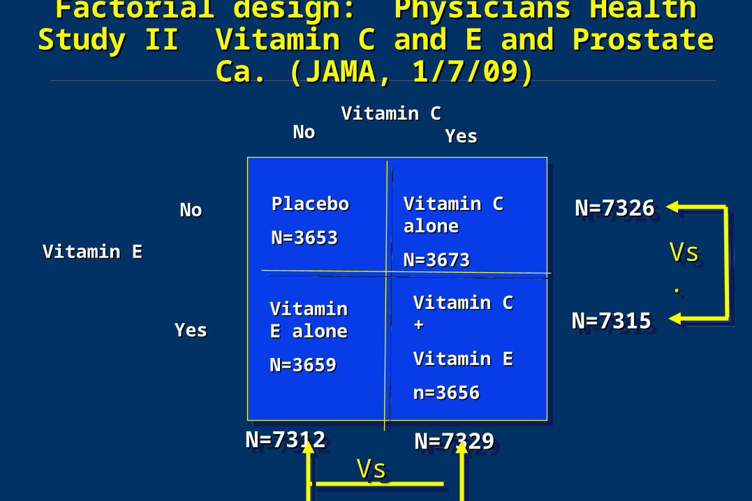
Factorial design: Physicians Health Study II Factorial design: Physicians Health Study II Vitamin C and E and Prostate Ca. (JAMA, 1/7/09)Vitamin C and E and Prostate Ca. (JAMA, 1/7/09)
Vitamin E Vitamin E + C+ CVitamin E Vitamin E + C+ C
Vitamin E Vitamin E alonealoneVitamin E Vitamin E alonealone
Vitamin C Vitamin C alonealoneVitamin C Vitamin C alonealone
Placebos Placebos onlyonlyPlacebos Placebos onlyonly
From Figure 1 from Gaziano et alFrom Figure 1 from Gaziano et alFrom Figure 1 from Gaziano et alFrom Figure 1 from Gaziano et al

Factorial design: Physicians Health Study II Factorial design: Physicians Health Study II Vitamin C and E and Prostate Ca. (JAMA, 1/7/09)Vitamin C and E and Prostate Ca. (JAMA, 1/7/09)
PlaceboPlacebo
N=3653N=3653
Vitamin E Vitamin E alonealone
N=3659N=3659
Vitamin C Vitamin C alonealone
N=3673N=3673
Vitamin C + Vitamin C +
Vitamin EVitamin E
n=3656n=3656
N=7326N=7326N=7326N=7326
Vitamin EVitamin E
NoNo
YesYes
NoNo YesYesVitamin CVitamin C
N=7315N=7315N=7315N=7315
N=7312N=7312N=7312N=7312 N=7329N=7329N=7329N=7329
Vs.Vs.Vs.Vs.
Vs.Vs.Vs.Vs.

Factorial design: Physicians Health Study II Factorial design: Physicians Health Study II Vitamin C and E and Prostate Ca. (JAMA, 1/7/09)Vitamin C and E and Prostate Ca. (JAMA, 1/7/09)

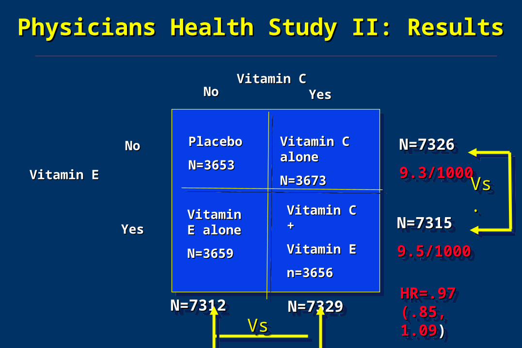
Physicians Health Study II: Results for Vit EPhysicians Health Study II: Results for Vit E
PlaceboPlacebo
N=3653N=3653
Vitamin E Vitamin E alonealone
N=3659N=3659
Vitamin C Vitamin C alonealone
N=3673N=3673
Vitamin C + Vitamin C +
Vitamin EVitamin E
n=3656n=3656
N=7326N=7326
9.3/10009.3/1000
N=7326N=7326
9.3/10009.3/1000Vitamin EVitamin E
NoNo
YesYes
NoNo YesYesVitamin CVitamin C
N=7315N=7315
9.5/10009.5/1000
N=7315N=7315
9.5/10009.5/1000
N=7312N=7312N=7312N=7312 N=7329N=7329N=7329N=7329
Vs.Vs.Vs.Vs.
Vs.Vs.Vs.Vs.
HR=.97 HR=.97 (.85, 1.09(.85, 1.09))
HR=.97 HR=.97 (.85, 1.09(.85, 1.09))

Factorial design example results: Factorial design example results: No interaction between treatmentsNo interaction between treatments
10%10%
8%8%
6%6%
4.8%4.8%
Vitamin EVitamin E
NoNo
YesYes
NoNo YesYesVitamin CVitamin C
40% 40% reduction for reduction for Vitamin CVitamin C
40% 40% reduction for reduction for vitamin Cvitamin C
20% 20% reduction for reduction for Vitamin EVitamin E
20% 20% reduction for reduction for Vitamin EVitamin E

Factorial design: Interaction between Factorial design: Interaction between treatmentstreatments
10%10%
8%8%
6%6%
4.8%4.8%
10%10%
Vitamin EVitamin E
NoNo
YesYes
NoNo YesYesVitamin CVitamin C
40% 40% reduction for reduction for Vitamin CVitamin C
20% increase 20% increase for vitamin Cfor vitamin C
20% 20% reduction for reduction for Vitamin EVitamin E
40% increase 40% increase for Vitamin Efor Vitamin E

Factorial design: Interaction between Factorial design: Interaction between treatmentstreatments
10%10%
8%8%
6%6%
Vitamin EVitamin E
NoNo
YesYes
NoNo YesYesVitamin CVitamin C
40% 40% reduction for reduction for Vitamin CVitamin C
90% 90% reduction for reduction for vitamin Cvitamin C
20% 20% reduction for reduction for Vitamin EVitamin E
~80% ~80% reduction for reduction for Vitamin EVitamin E
4.8%4.8%
1%1%

Factorial design: Analysis Implications Factorial design: Analysis Implications
• If you test for interactions and see none, simple comparison of If you test for interactions and see none, simple comparison of groupsgroups
• In prostate cancer paper end of results:In prostate cancer paper end of results:– “ “we examined 2 way interactions between vitamin C and E and found no we examined 2 way interactions between vitamin C and E and found no
interaction”interaction”
• Effect of vitamin C was the same regardless of whether or not Effect of vitamin C was the same regardless of whether or not they received vitamin Ethey received vitamin E
• Effect of vitamin E was the same regardless of whether or not Effect of vitamin E was the same regardless of whether or not they received vitamin Cthey received vitamin C
• Caution:Caution: test of interaction may be very low power test of interaction may be very low power
Physicians Health Study II: ResultsPhysicians Health Study II: Results
PlaceboPlacebo
N=3653N=3653
Vitamin E Vitamin E alonealone
N=3659N=3659
Vitamin C Vitamin C alonealone
N=3673N=3673
Vitamin C + Vitamin C +
Vitamin EVitamin E
n=3656n=3656
N=7326N=7326
9.3/10009.3/1000
N=7326N=7326
9.3/10009.3/1000Vitamin EVitamin E
NoNo
YesYes
NoNo YesYesVitamin CVitamin C
N=7315N=7315
9.5/10009.5/1000
N=7315N=7315
9.5/10009.5/1000
N=7312N=7312N=7312N=7312 N=7329N=7329N=7329N=7329
Vs.Vs.Vs.Vs.
Vs.Vs.Vs.Vs.
HR=.97 HR=.97 (.85, 1.09(.85, 1.09))
HR=.97 HR=.97 (.85, 1.09(.85, 1.09))

Factorial design: SELECT study Factorial design: SELECT study (Selenium and Vitamin E Trial) (Lippman) (Selenium and Vitamin E Trial) (Lippman)
(JAMA, 1/7/09)(JAMA, 1/7/09)
Vitamin E Vitamin E + + SeleniumSelenium
SeleniumSelenium
alonealone
Vitamin E Vitamin E
alonealoneplacebosplacebos

Factorial design: Factorial design: Alternative methods of data analysisAlternative methods of data analysis
• Assume that there are interactionsAssume that there are interactions
• Don’t collapse treatment groupsDon’t collapse treatment groups

Factorial design: SELECT study (Lippman) Factorial design: SELECT study (Lippman) (JAMA, 1/7/09)(JAMA, 1/7/09)
PlaceboPlacebo
Vitamin E Vitamin E alonealone
Selenium Selenium alonealone
Selenium + Selenium +
Vitamin EVitamin E
Vitamin Vitamin
EE
NoNo
YesYes
NoNo YesYesSeleniumSelenium
5 hypotheses 5 hypotheses each tested each tested at 0.005 (one at 0.005 (one sided). Why sided). Why not .05?not .05?
To adjust for To adjust for multiple multiple comparisonscomparisons

Factorial design: SELECT study (Lippman) Factorial design: SELECT study (Lippman) (JAMA, 1/7/09)(JAMA, 1/7/09)
PlaceboPlacebo
Vitamin E Vitamin E alonealone
Selenium Selenium alonealone
Selenium + Selenium +
Vitamin EVitamin E
Vitamin Vitamin
EE
NoNo
YesYes
NoNo YesYesSeleniumSelenium
Advantages/disad-Advantages/disad-vantages of this vantages of this analysis approach?analysis approach?

Factorial Designs: Data Analysis SummaryFactorial Designs: Data Analysis Summary
• Factorial design must be taken into account in analysis
• Many different approaches but should be thought out in advance
• Tests for interactions have low power and may negate some advantages of factorial design

Cross Over Designs: Analysis Implications Cross Over Designs: Analysis Implications
• Cross-over designs– Subject is own control
• Example: paroxetine and menopausal symptoms
– Good design when within-person variation is small
– Interpretation requires (mild) assumptions• 1. No effect of order to treatments: a then b is same as b then a• 2. No carryover effect (need long enough wash out period)
– Can test for effect of order via model with interaction but large sample size required
– Model:• treatment• order of treatments• treatment by order interactionn

Paroxetine for Hot Flashes Paroxetine for Hot Flashes (Sterns et al from section)(Sterns et al from section)

Advanced Topics in Data Analysis Advanced Topics in Data Analysis for Clinical Trialsfor Clinical Trials
• SubgroupsSubgroups
• Adjustment for baseline covariables (later)Adjustment for baseline covariables (later)
• Multiple endpointsMultiple endpoints
• Analysis of adverse eventsAnalysis of adverse events
• Interim analysisInterim analysis
Multiple Comparisons
Multiple Comparisons
Multiple Comparisons
Multiple ComparisonsA digression….A digression….A digression….A digression….

Multiple comparisonsMultiple comparisons
• The general problemThe general problem– Each statistical test has a 5% chance of Type I errorEach statistical test has a 5% chance of Type I error
– We are wrong 1 time out of 20We are wrong 1 time out of 20
– Easy to come up with spurious resultsEasy to come up with spurious results
• Take a worthless drug (placebo 2) compare to placebo 1Take a worthless drug (placebo 2) compare to placebo 1– 1 study: P(type I error)= 5%1 study: P(type I error)= 5%
– 2 studies: P(1 or 2 type I errors)= almost 10%2 studies: P(1 or 2 type I errors)= almost 10%
– 20 studies: P(at least one significant)=64%20 studies: P(at least one significant)=64%
• Publication biasPublication bias
• (Huge problem in genetics studies)(Huge problem in genetics studies)
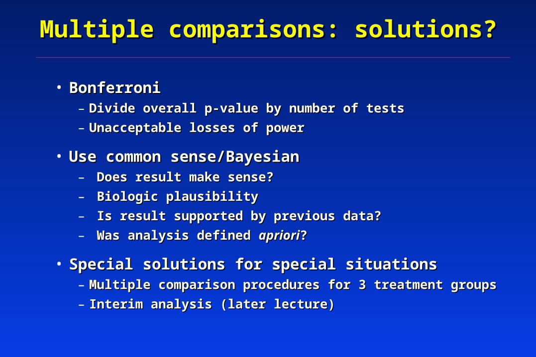
Multiple comparisons: solutions?Multiple comparisons: solutions?
• BonferroniBonferroni– Divide overall p-value by number of testsDivide overall p-value by number of tests
– Unacceptable losses of powerUnacceptable losses of power
• Use common sense/BayesianUse common sense/Bayesian– Does result make sense?Does result make sense?
– Biologic plausibilityBiologic plausibility
– Is result supported by previous data?Is result supported by previous data?
– Was analysis defined Was analysis defined aprioriapriori??
• Special solutions for special situationsSpecial solutions for special situations– Multiple comparison procedures for 3 treatment groupsMultiple comparison procedures for 3 treatment groups
– Interim analysis (later lecture)Interim analysis (later lecture)

Advanced Topics in Data Analysis Advanced Topics in Data Analysis for Clinical Trialsfor Clinical Trials
• SubgroupsSubgroups
• Adjustment for baseline covariables (later)Adjustment for baseline covariables (later)
• Multiple endpointsMultiple endpoints
• Analysis of adverse eventsAnalysis of adverse events
• Interim analysisInterim analysis

SubgroupsSubgroups
• After primary analysis, often want to look at After primary analysis, often want to look at subgroupssubgroups
• Does effectiveness vary by subgroupDoes effectiveness vary by subgroup
• If drug effective, is it more effective in some If drug effective, is it more effective in some populations?populations?
• If results overall show no effect, does drug work in If results overall show no effect, does drug work in subgroup of participants?subgroup of participants?
• Are adverse effects concentrated in some Are adverse effects concentrated in some subgroups?subgroups?

Levels of subgroups (from FFD)Levels of subgroups (from FFD)
1. 1. Those specified in study protocol have Those specified in study protocol have highest validityhighest validityEspecially if number is smallEspecially if number is small
2. Those implied by study protocol2. Those implied by study protocoleg. If randomization stratified by age, sex or disease stageeg. If randomization stratified by age, sex or disease stage
3. Subgroups suggested by other trials3. Subgroups suggested by other trials
4. (Weakest) Subgroups suggested by the data 4. (Weakest) Subgroups suggested by the data themselves (“fishing” or “data dredging”)themselves (“fishing” or “data dredging”)
5. (Diastrous) Subgroups based on post-randomization 5. (Diastrous) Subgroups based on post-randomization variablesvariables

Case Study: Efficacy of Alendronate On Case Study: Efficacy of Alendronate On Reducing Clinical FracturesReducing Clinical Fractures
• Fracture Intervention Trial (FIT) II: Women Fracture Intervention Trial (FIT) II: Women with BMD T-score < -1.6 (osteopenic--only with BMD T-score < -1.6 (osteopenic--only 1/3 osteoporotic)1/3 osteoporotic)–Primary endpoint: non-vertebral fracturesPrimary endpoint: non-vertebral fractures
• Overall results: Overall results: –14% reduction in non-vertebral fractures 14% reduction in non-vertebral fractures
(p=.07)(p=.07)
–WimpyWimpy
Cummings, Black et. al, JAMA, 1997Cummings, Black et. al, JAMA, 1997

RR for non-vertebral fracture of alendronateRR for non-vertebral fracture of alendronate(FIT II, Cummings, JAMA 1999) (FIT II, Cummings, JAMA 1999)
BB
BB
BB
00
11
1.51.5
OverallOverall
0.860.86(0.73 - 1.01)(0.73 - 1.01)
Re
lati
ve
Ris
kR
ela
tiv
e R
isk P=0.07P=0.07P=0.07P=0.07
Cummings, Black et. al, JAMA, 1997Cummings, Black et. al, JAMA, 1997

Reduction in non-spine fracture of Reduction in non-spine fracture of alendronate by baseline BMD groupsalendronate by baseline BMD groups
BB
BB
BB
BB
BB
BB
BB
BB
BB
BB
BB
BB
00
11
1.51.5
Baseline Femoral Neck BMD, by T-scoreBaseline Femoral Neck BMD, by T-score
OverallOverall T < -2.5T < -2.5 -2.5 < T < -2.0-2.5 < T < -2.0 T > -2.0T > -2.0
RH=0.86RH=0.86(0.73 - 1.01)(0.73 - 1.01)
RH=0.64RH=0.64(0.50 - 0.82)(0.50 - 0.82)
RH=1.03RH=1.03
(0.77 - 1.39)(0.77 - 1.39)
RH=1.14RH=1.14 (0.82 - 1.60)(0.82 - 1.60)
Re
lati
ve
Ris
kR
ela
tiv
e R
isk
Cummings, Black et. al, JAMA, 1997Cummings, Black et. al, JAMA, 1997

Data Analysis of Subgroup ResultsData Analysis of Subgroup Results
2 important components:2 important components:
- 1. Test for interaction- 1. Test for interactionIs RH equal at all levels of covariate (BMD)Is RH equal at all levels of covariate (BMD)
- 2. Also look at significance within subgroup- 2. Also look at significance within subgroup

Reduction in non-spine fracture of Reduction in non-spine fracture of alendronate by baseline BMD groupsalendronate by baseline BMD groups
BB
BB
BB
BB
BB
BB
BB
BB
BB
BB
BB
BB
00
11
1.51.5
Baseline Femoral Neck BMD, by T-scoreBaseline Femoral Neck BMD, by T-score
OverallOverall T < -2.5T < -2.5 -2.5 < T < -2.0-2.5 < T < -2.0 T > -2.0T > -2.0
RH=0.86RH=0.86(0.73 - 1.01)(0.73 - 1.01)
RH=0.64RH=0.64(0.50 - 0.82)(0.50 - 0.82)
RH=1.03RH=1.03
(0.77 - 1.39)(0.77 - 1.39)
RH=1.14RH=1.14 (0.82 - 1.60)(0.82 - 1.60)
Re
lati
ve
Ris
kR
ela
tiv
e R
isk
Cummings, Black et. al, JAMA, 1997Cummings, Black et. al, JAMA, 1997
Interaction p=.01Interaction p=.01

What to Do With an What to Do With an Unexpected Subgroup FindingUnexpected Subgroup Finding
• Is this a real finding? Is this a real finding?
• Was it specified in protocol (with Was it specified in protocol (with smallsmall number of other number of other analyses specified)?analyses specified)?
• Has this been previously observed?Has this been previously observed?– Increase prior probabilityIncrease prior probability
• Ways to verifyWays to verify– Examine for other similar subgrouping variables (BMD at hip, spine, Examine for other similar subgrouping variables (BMD at hip, spine,
radius)radius)
– Examine for other similar endpoints (hip fractures, etc.)Examine for other similar endpoints (hip fractures, etc.)
– Consider biologic plausibilityConsider biologic plausibility
– Most important: other trials, if possible and availableMost important: other trials, if possible and available

Another alendronate trial:Another alendronate trial:Fosamax International Trial (FOSIT)Fosamax International Trial (FOSIT)
• 1908 women, 34 countries1908 women, 34 countries
• Alendronate vs. placeboAlendronate vs. placebo
• 47% reduction in all clinical fractures (p<.05)47% reduction in all clinical fractures (p<.05)

Effect of Alendronate on Non-spine Fx Depends on Baseline Hip BMD in FOSIT*
Baseline hip BMD T-score
Overall
< - 2.5
-2.0 – -2.5
> -2
0.1 1 10Relative Hazard (± 95% CI)
0.53 (0.3, 0.9)
0.26 (0.1, 0.7)
0.32 (.07, 1.5)
1.2 (0.5, 2.9)
*Black, Pols, et. al, IOF meeting, 5/02
BMD Interaction for non-spine fractureBMD Interaction for non-spine fracture
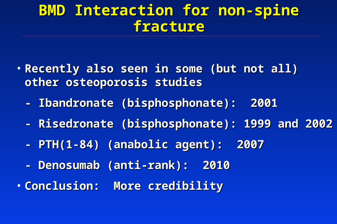
• Recently also seen in some (but not all) other Recently also seen in some (but not all) other osteoporosis studies osteoporosis studies
- Ibandronate (bisphosphonate): 2001- Ibandronate (bisphosphonate): 2001
- Risedronate (bisphosphonate): 1999 and 2002- Risedronate (bisphosphonate): 1999 and 2002
- PTH(1-84) (anabolic agent): 2007- PTH(1-84) (anabolic agent): 2007
- Denosumab (anti-rank): 2010- Denosumab (anti-rank): 2010
• Conclusion: More credibilityConclusion: More credibility

Subgroup Analysis During HERS for DSMBSubgroup Analysis During HERS for DSMB
• Look at impact of HRT in women with CHD Look at impact of HRT in women with CHD for new CHD (expected large reduction)for new CHD (expected large reduction)
• Overall no effect of HRT on CHD or Overall no effect of HRT on CHD or perhaps harm in early resultsperhaps harm in early results
• Is there subgroup with significant harm? Is there subgroup with significant harm? Might want to discontinue that subgroup.Might want to discontinue that subgroup.
• Look at relative hazard (RH) within Look at relative hazard (RH) within subgroups defined by baseline variable. subgroups defined by baseline variable. For DSMB during study…For DSMB during study…

Subgroup analysis for DSMB Subgroup analysis for DSMB during HERSduring HERS
•
Relative hazard (E vs. placebo)Relative hazard (E vs. placebo)
Subgroup Within AmongSubgroup Within Among
Subgroup N (%) Subgroup Others p (intrac)*Subgroup N (%) Subgroup Others p (intrac)*
history of smoking 1712 (62) 1.01 3.39history of smoking 1712 (62) 1.01 3.39 .01 .01
current smoker 360 (13) 0.55 1.92 .03 current smoker 360 (13) 0.55 1.92 .03
digitalis use 275 (10) 4.98 1.26 .04 digitalis use 275 (10) 4.98 1.26 .04
>= 3 live births 1616 (58) 1.09 2.72 .04 >= 3 live births 1616 (58) 1.09 2.72 .04
lives alone 775 (28) 2.97 1.14 .05 lives alone 775 (28) 2.97 1.14 .05
prior mi by chart review 1409 (51) 2.14 0.93 .05 prior mi by chart review 1409 (51) 2.14 0.93 .05
beta-blocker use 899 (33) 2.89 1.15 .06 beta-blocker use 899 (33) 2.89 1.15 .06
age >= 70 at randomization 1019 (37) 2.65 1.14 .06age >= 70 at randomization 1019 (37) 2.65 1.14 .06
*Statistical significance of interaction*Statistical significance of interaction
Dave DemetsDave DemetsDave DemetsDave Demets

Lots of subgroups were analyzed in HERSLots of subgroups were analyzed in HERS
• history of smoking (at rv) 1712 (62) 1.01 3.39 0.30 .01 history of smoking (at rv) 1712 (62) 1.01 3.39 0.30 .01 • current smoker (at rv) 360 (13) 0.55 1.92 0.29 .03 current smoker (at rv) 360 (13) 0.55 1.92 0.29 .03 • digitalis use (at rv) 275 (10) 4.98 1.26 3.96 .04 digitalis use (at rv) 275 (10) 4.98 1.26 3.96 .04 • >= 3 live births 1616 (58) 1.09 2.72 0.40 .04 >= 3 live births 1616 (58) 1.09 2.72 0.40 .04 • lives alone (at rv) 775 (28) 2.97 1.14 2.60 .05 lives alone (at rv) 775 (28) 2.97 1.14 2.60 .05 • prior mi by chart review (cr) 1409 (51) 2.14 0.93 2.30 .05 prior mi by chart review (cr) 1409 (51) 2.14 0.93 2.30 .05 • beta-blocker use (at rv) 899 (33) 2.89 1.15 2.51 .06 beta-blocker use (at rv) 899 (33) 2.89 1.15 2.51 .06 • age >= 70 at randomization 1019 (37) 2.65 1.14 2.32 .06 age >= 70 at randomization 1019 (37) 2.65 1.14 2.32 .06 • prior mi in most distant tertile 447 (16) 2.64 0.93 2.82 .07 prior mi in most distant tertile 447 (16) 2.64 0.93 2.82 .07 • walk 10m or in exercise program (at rv) 1770 (64) 2.35 1.11 2.12 .08 walk 10m or in exercise program (at rv) 1770 (64) 2.35 1.11 2.12 .08 • prior ptca by chart review (cr) 1189 (43) 0.92 1.98 0.46 .08 prior ptca by chart review (cr) 1189 (43) 0.92 1.98 0.46 .08 • prior mi within 2 years 420 (15) 3.20 1.28 2.50 .11 prior mi within 2 years 420 (15) 3.20 1.28 2.50 .11 • tg > median (at rv) 1377 (50) 2.02 1.05 1.93 .12 tg > median (at rv) 1377 (50) 2.02 1.05 1.93 .12 • rales in the lungs (at rv) 80 ( 3) 0.43 1.65 0.26 .13 rales in the lungs (at rv) 80 ( 3) 0.43 1.65 0.26 .13 • digitalis or ace-inhibitor use (at rv) 653 (24) 2.33 1.24 1.88 .16 digitalis or ace-inhibitor use (at rv) 653 (24) 2.33 1.24 1.88 .16 • previous ert for >= 12 months 302 (11) 4.19 1.41 2.98 .18 previous ert for >= 12 months 302 (11) 4.19 1.41 2.98 .18 • serious medical conditions 1028 (37) 1.05 1.81 0.58 .21 serious medical conditions 1028 (37) 1.05 1.81 0.58 .21 • age >= 53 at lmp 578 (21) 3.19 1.38 2.31 .23 age >= 53 at lmp 578 (21) 3.19 1.38 2.31 .23 • hdl > median (at rv) 1315 (48) 1.18 1.95 0.61 .24 hdl > median (at rv) 1315 (48) 1.18 1.95 0.61 .24 • lp(a) > median (at rv) 1378 (50) 1.26 2.08 0.60 .25 lp(a) > median (at rv) 1378 (50) 1.26 2.08 0.60 .25 • use of non-statin llm (at rv) 420 (15) 0.89 1.69 0.52 .25 use of non-statin llm (at rv) 420 (15) 0.89 1.69 0.52 .25 • married (at rv) 1588 (57) 1.26 1.98 0.64 .29 married (at rv) 1588 (57) 1.26 1.98 0.64 .29 • lvef <= 40% 178 ( 6) 2.16 1.01 2.13 .31 lvef <= 40% 178 ( 6) 2.16 1.01 2.13 .31 • prior mi within 4 years 765 (28) 2.07 1.32 1.57 .32 prior mi within 4 years 765 (28) 2.07 1.32 1.57 .32 • previous ert use for >= 1 year 327 (12) 2.86 1.41 2.03 .32 previous ert use for >= 1 year 327 (12) 2.86 1.41 2.03 .32 • prior mi within 1 year 194 ( 7) 2.88 1.43 2.02 .33 prior mi within 1 year 194 ( 7) 2.88 1.43 2.02 .33 • chest pain (at rv) 982 (36) 1.25 1.88 0.67 .33 chest pain (at rv) 982 (36) 1.25 1.88 0.67 .33 • dbp >= 90 mmhg (at rv) 149 ( 5) 0.91 1.62 0.56 .35 dbp >= 90 mmhg (at rv) 149 ( 5) 0.91 1.62 0.56 .35 • prior ptca within 1 year 206 ( 7) 3.94 1.46 2.71 .38 prior ptca within 1 year 206 ( 7) 3.94 1.46 2.71 .38 • prior mi within 3 years 612 (22) 2.05 1.37 1.50 .40 prior mi within 3 years 612 (22) 2.05 1.37 1.50 .40 • prior ptca within 4 years 838 (30) 1.15 1.70 0.68 .40 prior ptca within 4 years 838 (30) 1.15 1.70 0.68 .40 • use of any llm (at rv) 1296 (47) 1.23 1.76 0.70 .40 use of any llm (at rv) 1296 (47) 1.23 1.76 0.70 .40 • diuretic use (at rv) 775 (28) 1.89 1.33 1.42 .41 diuretic use (at rv) 775 (28) 1.89 1.33 1.42 .41 • signs and symptoms of chf (at rv) 118 ( 4) 0.94 1.60 0.58 .42 signs and symptoms of chf (at rv) 118 ( 4) 0.94 1.60 0.58 .42 • ace inhibitor use (at rv) 483 (17) 2.05 1.40 1.46 .44 ace inhibitor use (at rv) 483 (17) 2.05 1.40 1.46 .44 • total cholesterol > median (at rv) 1377 (50) 1.32 1.80 0.74 .47 total cholesterol > median (at rv) 1377 (50) 1.32 1.80 0.74 .47 • l-thyroxine use (at rv) 414 (15) 2.29 1.43 1.60 .47 l-thyroxine use (at rv) 414 (15) 2.29 1.43 1.60 .47 • poor/fair self-rated health (at rv) 665 (24) 1.30 1.72 0.76 .51 poor/fair self-rated health (at rv) 665 (24) 1.30 1.72 0.76 .51 • heart murmur (at rv) 540 (20) 1.89 1.42 1.34 .53 heart murmur (at rv) 540 (20) 1.89 1.42 1.34 .53 • sbp >= 140 mmhg (at rv) 1051 (38) 1.37 1.72 0.80 .59 sbp >= 140 mmhg (at rv) 1051 (38) 1.37 1.72 0.80 .59 • prior ptca within 3 years 695 (25) 1.27 1.61 0.78 .62 prior ptca within 3 years 695 (25) 1.27 1.61 0.78 .62 • s3 heart sounds (at rv) 19 ( 1) 2.74 1.50 1.82 .63 s3 heart sounds (at rv) 19 ( 1) 2.74 1.50 1.82 .63 • htn by physical exam (at rv) 557 (20) 1.32 1.62 0.81 .64 htn by physical exam (at rv) 557 (20) 1.32 1.62 0.81 .64 • >= 2 severely obstructed main vessels 1312 (47) 1.53 1.26 1.22 .69 >= 2 severely obstructed main vessels 1312 (47) 1.53 1.26 1.22 .69 • statin use (at rv) 1004 (36) 1.34 1.59 0.84 .71 statin use (at rv) 1004 (36) 1.34 1.59 0.84 .71 • have you ever been pregnant 2564 (93) 1.55 1.15 1.35 .72 have you ever been pregnant 2564 (93) 1.55 1.15 1.35 .72 • calcium-channel blocker (at rv) 1511 (55) 1.61 1.38 1.17 .73 calcium-channel blocker (at rv) 1511 (55) 1.61 1.38 1.17 .73 • previous hrt for >= least 12 months 132 ( 5) 1.24 1.60 0.78 .77 previous hrt for >= least 12 months 132 ( 5) 1.24 1.60 0.78 .77 • ldl > median (at rv) 1373 (50) 1.44 1.63 0.89 .77 ldl > median (at rv) 1373 (50) 1.44 1.63 0.89 .77 • prior ptca within 2 years 475 (17) 1.35 1.56 0.87 .81 prior ptca within 2 years 475 (17) 1.35 1.56 0.87 .81 • baseline left bundle branch block 212 ( 8) 1.31 1.55 0.85 .82 baseline left bundle branch block 212 ( 8) 1.31 1.55 0.85 .82 • white 2451 (89) 1.48 1.62 0.92 .88 white 2451 (89) 1.48 1.62 0.92 .88 • ever told you had diabetes 634 (23) 1.48 1.53 0.97 .94 ever told you had diabetes 634 (23) 1.48 1.53 0.97 .94 • aspirin use (at rv) 2183 (79) 1.51 1.56 0.97 .95 aspirin use (at rv) 2183 (79) 1.51 1.56 0.97 .95 • any alcohol consumption (at rv) 1081 (39) 1.54 1.57 0.98 .97 any alcohol consumption (at rv) 1081 (39) 1.54 1.57 0.98 .97 • gallstones or gallbladder dis. 633 (23) 1.55 1.52 1.02 .97 gallstones or gallbladder dis. 633 (23) 1.55 1.52 1.02 .97 •
baseline atrial fibrillation/flutter 33 ( 1) - 1.50baseline atrial fibrillation/flutter 33 ( 1) - 1.50 - - - -
Total subgroups examined: 102Total subgroups examined: 102
Total subgroups with p< .05: 6Total subgroups with p< .05: 6
Total subgroups examined: 102Total subgroups examined: 102
Total subgroups with p< .05: 6Total subgroups with p< .05: 6

Subgroups: many problemsSubgroups: many problems
• Subgroups are full of statistical problemsSubgroups are full of statistical problems– Multiple comparisons may lead to erroneous Multiple comparisons may lead to erroneous
conclusionsconclusions
• Limited power in for subgroup analysesLimited power in for subgroup analyses
• Subgroups based on baseline variables are less Subgroups based on baseline variables are less badbad
• Subgroups based on post-randomization Subgroups based on post-randomization variables are more problematicvariables are more problematic

Subgroups Recommendations in NEJMSubgroups Recommendations in NEJM(Wang et al)(Wang et al)

Subgroups Recommendations Subgroups Recommendations in NEJM (Wang, et. al)in NEJM (Wang, et. al)
• Methods. Indicate..Methods. Indicate..– Number of pre-specified subgroups analyzed and Number of pre-specified subgroups analyzed and
reportedreported
– Number of post-hoc..Number of post-hoc..
– Potential effect on Type I error. Formal adjustment? Potential effect on Type I error. Formal adjustment? Or ?Or ?
• ResultsResults– Base analyses on tests for interaction and present along Base analyses on tests for interaction and present along
with within-group effects and CIswith within-group effects and CIs
• DiscussionDiscussion– Avoid overinterpretationAvoid overinterpretation
– Review supporting/conflicting dataReview supporting/conflicting data

RCT: Do an Adjusted Analysis?RCT: Do an Adjusted Analysis?
• Could view RCT as a prospective trial with binary Could view RCT as a prospective trial with binary predictor (treatment)predictor (treatment)
• Use ANOVA or ANCOVA to adjust if a continuous Use ANOVA or ANCOVA to adjust if a continuous outcomeoutcome
• Could use logistic regression or Cox PH models to Could use logistic regression or Cox PH models to adjust if binary outcomeadjust if binary outcome
• General rule: Variable could be a confounder if it is General rule: Variable could be a confounder if it is related to both outcome and predictor (treatment)related to both outcome and predictor (treatment)
• Ok?Ok?

Adjusted analysis in a randomized trialAdjusted analysis in a randomized trial
- - What if important prognostic variables (confounders) What if important prognostic variables (confounders) are maldistributed by chance alone?are maldistributed by chance alone?
eg. Trial of MI: placebos older than treatedeg. Trial of MI: placebos older than treated
Adjust for age?Adjust for age?
- Controversial issue- Controversial issue
If you adjust for enough variables, you will eventually If you adjust for enough variables, you will eventually change the results. High potential for hanky-panky.change the results. High potential for hanky-panky.

Adjusted analysis in a randomized trialAdjusted analysis in a randomized trial
Potential solutions:Potential solutions:
• If a specific variable is highly prognostic, then If a specific variable is highly prognostic, then use stratified blocking to guarantee balanceuse stratified blocking to guarantee balance
• Perform analysis unadjusted and then adjustedPerform analysis unadjusted and then adjusted
• Pre-specify condition under which adjustment Pre-specify condition under which adjustment will be done for a small set of prognostic will be done for a small set of prognostic variables:variables:- eg. If age, BP or ldl are maldistributed (p<.05), then - eg. If age, BP or ldl are maldistributed (p<.05), then
adjust for that/those variable(s) only.adjust for that/those variable(s) only.

Other topics in Data Analysis of Clinical TrialsOther topics in Data Analysis of Clinical Trialsfor later lecturesfor later lectures
• Multiple endpointsMultiple endpoints
• Analysis of adverse eventsAnalysis of adverse events
• Interim analysisInterim analysis

Statistical issues: SummaryStatistical issues: Summary
• Main analysis generally straightforwardMain analysis generally straightforward– Based on two-group comparison tests or multi-group Based on two-group comparison tests or multi-group
generalizationsgeneralizations
• Special designs require special analysisSpecial designs require special analysis
• Multiple comparisons are ubiquitousMultiple comparisons are ubiquitous– MonitoringMonitoring
– Subgroup analysesSubgroup analyses
– Safety analysesSafety analyses
– Where possible, minimize subjectivity and adhoc-nessWhere possible, minimize subjectivity and adhoc-ness
– Try to replicate resultsTry to replicate results