some operational applications of geostatistics at hydro ... · some operational applications of...
TRANSCRIPT

Dominique TAPSOBAHydro-Québec’s research institute (IREQ),Varennes, Québec, CANADA
Some operational applications of geostatistics at Hydro-Québec
Université de MontréalNICDS Workshop “Statistical Methods for Geographic and Spatial Data in the Management of Natural Resources” March 3-5, 2010
Presentation outline
Hydro-Québec at a glance
Applied geostatistics for :Snow Water Equivalent (SWE) estimation over Hydro-Québec’s watersheds
Wind speed temporal variability analysis over the Gaspe Peninsula (preliminary analysis)
Results and validations
Conclusions
Future work

Focusing interest areas
SWE EstimationHydro-Quebéc’s Watersheds
Wind speed analysisGaspe Peninsula

Hydro-Québec at a glance
The main watersheds

Hydro-Québec at a glance
Generating facilities by watersheds
Hydroelectric generating stations1 TWh = 1,000,000,000 kWh

• Snow accumulation over Québec and Labrador represents the 2nd largest continental SWE maxima for North America after the western Cordillera
• Annual maximum snow accumulation averages 200-300 mm
• Important resource for hydroelectricity production - estimated that 1 mm of SWE in the headwaters of the Caniapiscau-La Grande hydro corridor is equivalent to $1M in hydro-electric power production (R. Roy, personal communication, 2006).
• Spatial and temporal limitations in both satellite data and in situ snow monitoring networks are a constraint to understanding variability and change in SWE over this region of North America
Mean March SWE, 1979-1997 (Brown et al., 2003; Atmosphere-Ocean, 41, 1-14).
SWE = amount of water stored in the snow pack usually expressed in mm
Geostatistics for SWE estimation at Hydro-Québec
Background

Geostatistics for SWE estimation at Hydro-Québec
BackgroundLarge interannual variability in SWE over the Hydro-electric corridor of Québec… can vary ± 50-100 mm between years
1965 1970 1975 1980 1985 1990 1995 2000 2005100
150
200
250
300
Mea
n m
onth
ly S
WE
(mm
)
Mean March SWE, La Grande Basin, Quebec
Mean March SWE from snow course observations (52-55°N, 70-77.5°W)

Provide a high quality grid dataset to investigate the spatial and temporal variability in SWE over HQ’s watersheds.
Documenting and understanding variability and change in SWE are important for: seasonal prediction, validation of climate models, and understanding how snow cover may change in the future.
For operational run-off and streamflow forecasts, the maximum SWE grid map generated prior to spring snowmelt is used to assess the a priori potential for getting large run-off and floods.
Used to update the snow-related state variables employed by our hydrological models, which forecast water inflows into reservoirs during spring.
Snow anomaly maps to provide timely and geographic pattern of SWE to assist decision-making related to water management for Hydropower generation.
Geostatistics for SWE estimation at Hydro-Québec

Snow sampling
Geostatistics for SWE estimation in Hydro-Québec
Data acquisition

Location of snow course observations with 10-years of data from March 01 1970-1979
19301935
19401945
19501955
19601965
19701975
19801985
19901995
20002005
1
10
100
1000
10000
# S
now
Cou
rse
Obs
erva
tions
Number of SWE Observations in Quebec & Adjacent Regions
0
5000
10000
15000
20000
25000
30000
1 3 5 7 9 11 13 15 17 19 21 23 25 27 29
Day of month
No.
of s
now
cou
rses
In situ snow course and snow depth observations:• most observations are concentrated over southern regions • most data available since ~1960• majority of observations are made on the 1st and 15th of each month• gridding SWE at 10-km resolution
Geostatistics for SWE estimation at Hydro-Québec: Data sets

Geostatistics for SWE estimation at Hydro-Québec: Methodology
External Drift Kriging technique
We adopt non-stationary geostatistical techniques such as External Drift Kriging (EDK) (Wackernagel, 1998; Chiles and Delfiner, 1999, p.355)
Integration of auxiliary information such as elevation, as a predictor variable strongly correlated with SWE.
more reasonable result in terms of the known physical relationships, which are imposed on the local mean by the elevation covariate.
Easier to implement than Co-Kriging, collocated-cokriging
There is a strong relationship between topography and SWE. Linear correlation coefficients between SWE and topography over the 1970-2005 period are greater than 0.6.
0 100 200 300 400 500 600 700 800 900
0
100
200
300
400
R= 0.6
March 15th 1970
SWE(
mm
)
Elevation(m)Elevation(m)
100 200 300 400 500 600
0
100
200
SWE(
mm
)February 15th 2003
R=0.8

Geostatistics for SWE estimation at Hydro-Québec: MethodologyExternal Drift Kriging technique
External drift kriging (EDK) is a classical approach that aims at integrating, in the modeling of a target variable Z(x), the knowledge of an auxiliary field s(x) linearly correlated with Z(x), s(x) providing a large scale information about the spatial trend of Z(x). EDK only requires the kwnoledge of the variogram of the residuals (see e.g. Chilès & Delfiner, 1999).
In the case of the snow water equivalent (SWE), EDK at a given location x relies on the following decomposition:
with:
– D(x) derived from topography T(x):
– R(x) stationary residuals with mean 0.
To ensure robustness of the temporal SWE estimates, a constant variogram model is assumed for each season, fitted on average empirical variograms derived from the 1st and 15th of every month from December to May for the period from 1970 to 2005.
)()()( xRxDxSWE +=
bxaTxD += )()(

Geostatistics for SWE estimation at Hydro-Québec: MethodologyExternal Drift Kriging techniqueSWE spatio-temporal variability
Example of normalized variograms of residuals from SWE regression with topography (1970-1980).No significant differences in the global shape between monthly variograms.
JANUARY
0 100 200 300 400
Distance (km)
0.00
0.25
0.50
0.75
1.00
Variogram: Residuals
FEBRUARY
0 100 200 300 400
Distance (km)
0.00
0.25
0.50
0.75
1.00
Variogram: Residuals
MARCH
0 100 200 300 400
Distance (km)
0.00
0.25
0.50
0.75
1.00
Variogram: Residuals
0 100 200 300 400 500 600 700
Distance (km)
0.00
0.25
0.50
0.75
1.00
Variogram: Residuals Combined use of two model variograms focusing
on small and large distances for variogram fitting.
Choice of a variogram model based on two spherical nested structures

Geostatistics for SWE estimation at Hydro-Québec: Results
EDK shows a realistic spatial structure consistent with the structure of DEM but with SWE values honouring observation sites.
Polygonal technique was formerly used to generate Hydro-Québec forecasts. This technique was just based on the influence zone of each SWE measurement, without any additional information and any uncertainty estimate.
Maps of SWE spatial distribution for February 25th 2008 over Hydro-Quebec River basins: polygonal technique, SWE estimate usingelevation as external drift, standard deviation, anomaly in % (value minus reference period 1971-2000).
SWE-EDKSWE-Thiessen
SWE-StDev SWE- Anomaly
DEM

Geostatistics for SWE estimation at Hydro-QuébecOperational application of interpolation methodology for real-time monitoring of SWE.
SWE-EDK SWE-Stdev
Difference between current observed interpolated SWE map and the mean map (anomaly)
SWE anomaly maps are generated automatically bi-weekly from December to May to provide temporal information on the spatial distribution of SWE for decision-makers at Hydro-Québec.
Graphical User Interface Design for SWE estimation Over Hydro-Quebec River Basins (Internet website)
SWE-ANOMALY

Geostatistics for SWE estimation at Hydro-QuébecValidations
• Cross-validation carried out for March 15 (approx date of max annual SWE for most of Quebec) for a random selection of 25% of the observations (~130 observations/yr) over the 1970-2005 period
• rmse computed for interpolation results with EDK and a simple interpolation procedure (Thiessen polygon method) formely used as a reference
Conclusions:
• EDK had lower rmse than ThiessenEDK Thiessen
rmse (mm)1970-2005
33.6 44.5
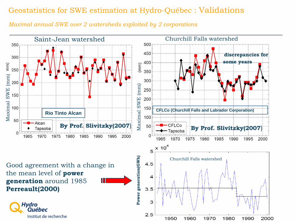
Geostatistics for SWE estimation at Hydro-Québec : Validations
Maximal annual SWE over 2 watersheds exploited by 2 corporations
By Prof. Slivitzky(2007) Max
imal
SW
E (m
m)
Max
imal
SW
E (m
m)
Rio Tinto Alcan CFLCo (Churchill Falls and Labrador Corporation)
discrepancies forsome years
Churchill Falls watershedSaint-Jean watershed
Pow
er g
ener
atio
n(G
Wh) Churchill Falls watershed
Good agreement with a change in the mean level of power generation around 1985 Perreault(2000)
By Prof. Slivitzky(2007)

Geostatistics for SWE estimation at Hydro-Québec
Uncertainty analysis
Essentially kriging produces:a simple map of the «best » local estimates a mean squared prediction error
Estimates are “smoothed” such that low values will tend to be overestimated and high values will tend to be underestimated
Deleterious consequences forModeling variabilityQuantifying uncertainty in the predictionUnderstanding risk
We use geostatistical simulation to produce multiple realizations all honouring the data and the statistics derived from the data

Geostatistics for SWE estimation at Hydro-Québec
Uncertainty analysis
Model uncertainty by generating a set of maps of the spatial distribution of SWE values. For this analysis, we generated 200realizations by Turning Bands technique (Journel, 1974; Chilès, 1977, Tompson et al., 1989)
Each realization is conditional to the original data and approximately reproduces the spatially weighted sample frequency distribution and the variogram. Therefore, the set of mean SWE values generated will be similar to that of kriging.
The Turning Bands algorithm used here assumes the data are normally distributed, although other probability models (including nonparametric) could be selected.
Journel ,(1974) Simulation Conditionnelle. Théories Pratique, thèse de Docteur-Ingénieur, Université de Nancy Chilès, J.P.(1977). Géostatistique des phénomènes non stationnaires. Thes, Doct.-Ing. Nancy.Tompson A.F.B. Abadou R.and Gelhar L. W.(1989). Implementation of a three-domensional Turning Bands random field generator, W.Ress.Res., Vol.25, no10, p.2227-2243

Geostatistics for SWE estimation at Hydro-Québec
Uncertainty analysis (Ex: Kenogami river basin 3390km2)
740 750 760 770 780 790 800 740 750 760 770 780 790 800 740 750 760 770 780 790 800 740 750 760 770 780 790 800
X (km)
5280
5290
5300
5310
5320
5330
5340
5350
5360
5370
Y (km)
740 750 760 770 780 790 800 740 750 760 770 780 790 800
Exp. 6 simulated realizations of SWE
40.037.535.032.530.027.525.022.520.017.515.012.510.0
740 750 760 770 780 790 800
SWE(cm)DEM
Elev.(m) SWE_Estimation with EDK
Ex. March 31 1999
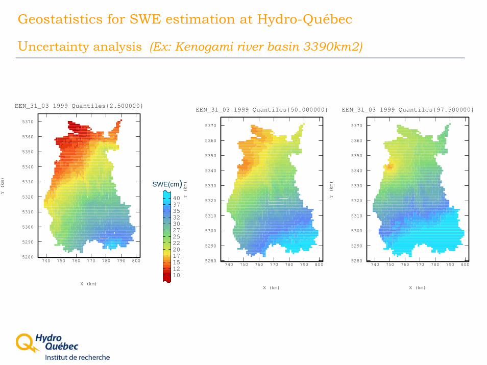
Geostatistics for SWE estimation at Hydro-Québec
Uncertainty analysis (Ex: Kenogami river basin 3390km2)
740 750 760 770 780 790 800
X (km)
5280
5290
5300
5310
5320
5330
5340
5350
5360
5370
Y (km)
EEN_31_03 1999 Quantiles{2.500000}
40.037.535.032.530.027.525.022.520.017.515.012.510.0
740 750 760 770 780 790 800
X (km)
5280
5290
5300
5310
5320
5330
5340
5350
5360
5370
Y (km)
EEN_31_03 1999 Quantiles{50.000000}
740 750 760 770 780 790 800
X (km)
5280
5290
5300
5310
5320
5330
5340
5350
5360
5370
Y (km)
EEN_31_03 1999 Quantiles{97.500000}
SWE(cm)

Geostatistical analysis of wind speed temporal variability
Background
Integrating wind power into a large, primarily hydroelectric generating fleet presents a real challenge. Hydro-Québec is therefore developing cutting-edge expertise in order to:
Plan the integration of wind farms into its grid
Develop method to characterize and forecast fluctuating wind power output (in collaboration with Environment Canada) that will maximize the contribution of wind energy without compromising the reliability of the transport
Maintain safe, reliable operation of the power system

Geostatistical analysis of wind speed temporal variability
Background

Geostatistical analysis of wind speed temporal variability
Wind speed is essential for wind power generation however :
Wind speed varies quickly in time and the power output is dependent on how fast the wind is blowing. Therefore, it is desirable that wind speed temporal variability (patterns) be investigated and described
One way for predicting a wind farm power would be forecast wind speed through a numerical weather prediction (NWP) model and convert them into a production value by means of a wind farm power curve. Therefore it could be interesting to analyse NWP Outputs and observations
A simple equation for the Power in the Wind P
P = 1/2 ρ Π r2 V3
ρ = Density of the Airr = Radius of your swept areaV = Wind Velocity
Power is proportional to theCUBE of wind speed

Geostatistical analysis of wind speed temporal variability
The purpose of the study
Extract the maximum information of wind speed time series properties over an area of interest using geostatistical framework.
There are different ways to do that, such are spectral methods, wavelets but we focus here on the semivariogram method for its robustness.
For wind power generation, the mean behaviour of wind speed over a time period (month, annual) for a given area (farm) is essential. We apply geostatistical tools, namely Mean Regional Temporal Semivariogram (MRTS) to capture the structure.
MRTS is also a way to ensure the robustness of semivariogram inference
Compare the temporal variability of wind speed recorded at the 10m meteorological stations and the GEM-LAM (Global Environmental MultiscaleLimited Area Model) model outputs.

Geostatistical analysis of wind speed temporal variability: Methodology
Mean regional temporal semivariograms (MRTS) definition and computation
Given N data points z1, z2,…, sampled at a regular interval d, the sample variogram can be computed for any lag h=kd, k=1, 2,…, by
Mean Regional Temporals Variogram is computed by:
∑=
=P
jkdR j
P 1
)(1 γγ
Where P is the number of stations within the area R
Rγ
∑=
=kdN
ikdstationkd N
j12
1)(γ

Geostatistical analysis of wind speed temporal variability
Application of MRTS to wind speed analysis
300 400 500 600 700 800 900 1000 110
X (km)
4900
5000
5100
5200
5300
5400
5500
5600
Y (km)
GEM-LAM 2.5km+ 10m sites
V(m/s)
10
9
8
7
6
5
4
3
2
1
0
01/01/2009-11h
Environment Canada records a wind velocity (speed and direction) at every hour at 41 sites at 10m
Estimates GEM-LAM value at station locations using a bilinear method(SMC)
GEM-LAM= Global Environmental Multiscale Limited Area ModelNumerical model employed operationally by Environment Canada’s – Canadian Meteorological Centre (CMC)
•forecast periods up to 24 hours•initial and boundary conditions derived from CMC’s operational regional GEM 15 km resolution forecast system (GEM 15).•presently run for two configurations: SW Canada/Pacific Northwest, and southern Ontario and Québec
Data and domain

Geostatistical analysis of wind speed temporal variability
MRTS - Observations 2001
June July August September
January October November December
February March April May

Geostatistical analysis of wind speed temporal variability
MRTS - Observations 2007
June July August September
January October November December
February March April May

Geostatistical analysis of wind speed temporal variability
MRTS –FITTING
Tapsoba Dominique. Regional-temporal patterns of wind speed over the Gaspe peninsula suggested by 1-D Variogram. (Renewable Energy)
Time (heure)
Ex: May 2007
Var
iogr
am Choice of a variogram model based on two (spherical and exponential cosine) nested structures

Geostatistical analysis of wind speed temporal variability
How well did the GEM-LAM capture the hourly variability of wind speed?
Hourly mean wind speed bias (Obs minus GEM-LAM Ouputs)

Geostatistical analysis of wind speed temporal variability
MRTS – Observations and GEM-LAM Outputs 2009
observation
GEM-LAM
Cross Vario

Geostatistical analysis of wind speed temporal variability
MRTS – Observations and GEM-LAM Outputs 2009va
riog
ram
vari
ogra
m
Time(h) Time(h)
observation
GEM-LAM
GEM-Cross Vario

Geostatistical analysis of wind speed temporal variability
MRTS – Observations and GEM-LAM Outputs 2009
observation
GEM-LAM
Cross Vario

Geostatistical analysis of wind speed temporal variability
MRTS – Observations and GEM-LAM Outputs 2009
observation
GEM-LAM
Cross Vario

Geostatistical analysis of wind speed temporal variability
MRTS – Observations and GEM-LAM Outputs 2009
MRTS method allows to characterize timescalesof wind speed varying signals
MRTS clearly show for the observations and the GEM-LAM model output a periodic component of 24h during summer
– For several years– For such behaviour have physical explanations
Both MRTS and GEM-LAM variograms do not show a clearly periodic signal during winter
GEM-LAM model systematically underestimated wind speed variability through time

Terminal conclusions : Future work
SWE estimation
Will investigate the usefulness of additional covariates e.g. vegetation characteristics (e.g. vegetation density and tree type play an important role in sublimation loss)
Take into account of an uncertainty of the variogram model parameters

Terminal conclusions : Future work
Wind speed variability analysis
We have to continue to study the wind speed behaviour both spatially and temporally in order to predict the wind characteristics at a specific farm from the general characteristics appropriate for a region.
Combine temporal and spatial models in order to correct the GEM-LAM Outputs.

Merci
• Ministère du Développement durable, de l'Environnement et des Parcs
• Ontario Ministry of Natural Resources
• New Brunswick Environment
• Environment Canada
Thanks to the data providers: