some questions and open problems in continuum mechanics ... · journal of differential equations...

JOURNAL OF DIFFERENTIAL EQUATIONS 48, 293-312 (1983)

Some Questions and Open Problems in

Continuum Mechanics and Population Dynamics

MORTON E. GURTIN

Department of Mathematics, Carnegie-Mellon University, Pittsburgh, Pennsylvania 152I3

Received October 30, 1981

This article presents some problems in continuum mechanics and population dynamics which are as yet unsolved, and which seem of interest, both from a mathematical and from a physical point of view.

The first problem concerns the buckling of a viscoelastic, Euler-Bernoulli beam. The resulting system of equations forms a nonlinear eigenvalue problem, but because of viscoelastic effects the buckled state depends on the history of the loading. This rate dependence renders the problem quite difficult. One cannot describe the results in terms of a simple bifurcation diagram, and at a bifurcation the preferred path is not immediate, as there is no obvious choice of energy.

Next, we discuss the problem of minimizing the residual stress that occurs during the cooling of a constrained viscoelastic material. What makes the problem interesting is the lack of convexity of the underlying cost function.

Our third problem deals with the dispersal (diffusion) of age-dependent biological populations. The general initial-value problem, which is open, is formulated. Under certain simplifying assumptions the general system reduces to a pair of reaction-diffusion equations with both reaction and diffusion terms nonlinear; these equations are in some ways degenerate parabolic, in other ways hyperbolic. The corresponding initial- value problem-with compactly supported data-is open. This problem, to me, seems unusually interesting.

Our final topic concerns population models whose basic equations are in some sense close to an iterated map of the form shown in Fig. 1 (Section 4). As is known, such iterated maps can yield chaotic behavior; a careful study of the perturbed systems might therefore lead to a better understanding of the onset of chaos.

293 0022-0396183 $3.00

Copyright 0 1983 by Academic Press, Inc. All rights of reproduction in any form reserved.

294 MORTON E.GURTIN

1. VISCOELASTIC BUCKLING: AN EIGENVALUE PROBLEM WHOSE EIGENVALUES ARE FUNCTIONS

A. Formulation of the Problem

Consider a thin, inextensible rod, pinned’ at the ends, and acted on by an axial end thrust P(t) in such a way that its center-line bends in a plane. Label material points by their positions x E [0, l] in the undeformed, straight configuration the rod is assumed to be in prior to time zero. For each material point x and time t, let m(x, t) denote the bending moment and u(x, t) the angle between the undeformed axis and the tangent to the rod at x. Then, as is tacit,

u(x, t) = m(x, t) = P(t) = 0 for t < 0.

We work within the quasi-static theory; thus balance of moments has the form (cf. e.g., Love [2, Sect. 2621)

m’+Psinu=O, (l-1)

where ’ = a/ax. We assume that the rod is linearly viscoelastic in the sense of the constitutive equation

m(x, t) = Pu’(x, t)+ ‘qt-S)U’(X,S)dS I (1.2) II

giving the bending moment as a function of the past history of the curvature u’. Here p > 0 is the instantaneous flexural rigidity, while A, assumed continuous and (0, measures internal dissipation. Without loss in generality we take p= 1; this simply amounts to replacing m, P, and 1 in (1.1) and (1.2) by m/P, Pip, and n//I, respectively. Thus (1.2) takes the form

m = u’ + A * u’, (1.3)

where we have used the standard notation for convolution. Equations (1.1) and (1.3) yield the integro-differential equation

u”+A*u”+Psinu=O.

Since the ends of the rod are pinned, the relevant boundary conditions are

m(0, t) = m( 1, t) = 0,

’ The results discussed here are valid for any of the standard boundary conditions. (In this connection, cf. Reynolds Ill.)

SOME QUESTIONS AND OPEN PROBLEMS 295

or, by (1.3) and the uniqueness theorem for Volterra integral equations,

u’(0, t) = u’(1, t) = 0.

Further, as the end of the rod at x = 1 can move only horizontally, we have the additional constraint

I 1

sin 24(x, t) dx = 0. 0

Summarizing, the viscoelastic (buckling) problem consists in finding functions P(t) and u(x, t) such that

u”+il*u”+Psinu=O,

u’(0, t) = u’(l, t) = 0,

I 1

sin u(x, t) dx = 0. (V) 0

The corresponding linear theory, appropriate to deformations with u small, is obtained by replacing sin u by u in the above equations. The resulting linearized viscoelastic problem therefore has the form’

u”+A*u”+Pu=O,

u’(0, t) = u’(l, t) = 0,

I 1

u(x, t) dx = 0. (LV 0

At this point it is convenient to also record the associated linearized elastic problem, which consists in finding constants P and functions u(x) such that

u”+Pu=O,

u’(0) = u’( 1) = 0,

( 1

u(x) dx = 0. 0

(W

The solutions, of course, are given by

u,(x) = cos n7q P, = n%*, n = 1, 2,....

2 Cf. Disttfano [3, 41 for a discussion of equations similar to (LV), . Disttfano restricts his attention to constant P, but includes a forcing term.

296 MORTON E. GURTIN

It is important to note that-in contrast to the elastic problem-the viscoelastic problem has “eigenvalues” P(t) which are functions of time t.

B. Results for the Linear Theory

The linearized viscoelastic problem has the following interesting features (Gurtin et al. [5]) not shared by the associated elastic problem:

(a) There do not exist buckled solutions with P(t) = constant for t > 0. (We use the term “buckled” as a synonym for “nontrivial.“)

(b) For each value of n there is-even modulo multiplicative constants-an uncountably infinite number of buckled solutions of the form

u(x, t) = y(t) cos n7z.x. (1.4)

In fact, any T > 0 and any function y on [0, T) for which the expression

w> r(t) + A * r(t) -= pn r(t)

exists on [0, r) yields-via (1.4)--- a buckled solution with P(t) the corresponding axial thrust.

One can also ask what axial thrusts P(t) yield buckled solutions. For the linearized problem (LV) the answer is furnished by the following results of Reynolds [ 11:

(c) If P(t) never equals an elastic buckling load P,, then there is no buckled solution corresponding to P.

(4 If

P(O) = P” 3 0 > P(0) > A(O) P, ,

then there exists a unique (modulo a multiplicative constant) buckled solution corresponding to P; if

P(0) = P, 3 P(0) < l(O) P, or P(0) > 0,

then there is no buckled solution corresponding to P. (Recall that A < 0.)

C. Questions and Open Problems

(1) Let A denote the operator

Au = -u” - 1 * u”.

Then the differential equation (LV), takes the form

@u)(t) = P(t) w, (1.5)


while the remaining conditions (LV),,, restrict the space in which ~(1) = u(., t) lives. Writing the linear problem in this manner leads one to ask whether there is a unified theory of eigenvalue problems of the form (1.5). One of the chief difficulties concerning (1.5) is that the operation of “multiplication” (for functions of time) which underlies the operator A is convolution, while the right side of (1.5) involves the usual pointwise product of functions.

(2) The nonlinear viscoelastic problem (V) remains open, although Reynolds [l] has established the local existence of buckled solutions for pP+) > p,, and has shown that only the trivial solutions u = nrr (n = 0, f l,...) are possible if P(t) < P, for all t. Here P, = x2 is the lowest eigenvalue of (LE). I conjecture the global existence of buckled solutions for any locally-bounded axial thrust P(t), 0 < t < co, with P(0 ’ ) > P, .

(3) (MacCamy, Reynolds) An interesting question concerns the equilibrium behavior of solutions to (V). Suppose that P(f) approaches a constant value ‘P,, as t --t co. Under what conditions will the solution u be approximated for large times by solutions of the nonlinear elastic problem corresponding to the differential equation

/I, w” + P, sin w = 0,

where /3, is the equilibrium modulus

so = 1 + iff n(s) ds.

(Here we assume that 1 E L’(0, co), /3,, > 0; note that, by (1.3), m/u’ -+ /I0 as t + 00 provided u’ has a limit.)

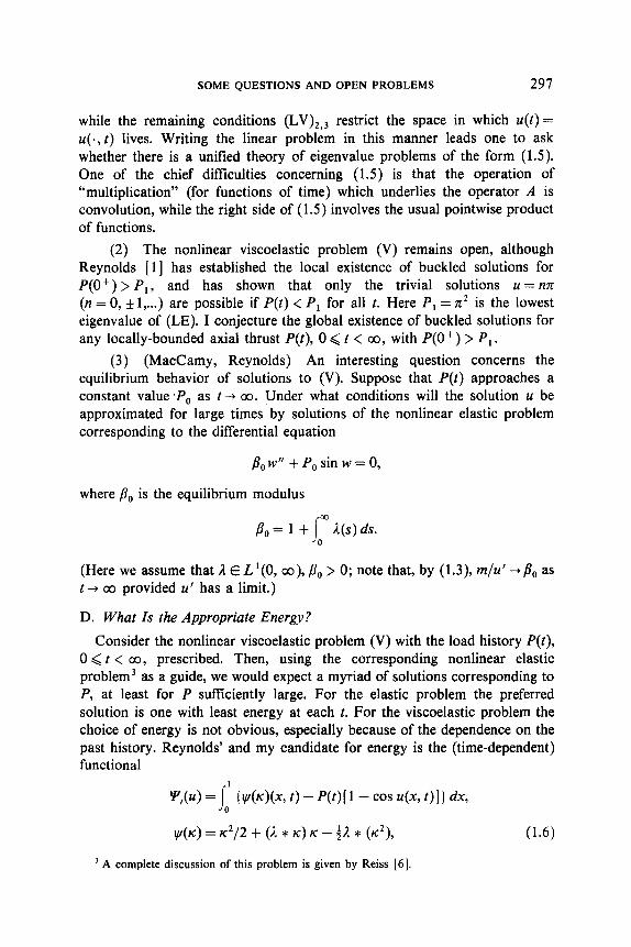
D. What Is the Appropriate Energy?

Consider the nonlinear viscoelastic problem (V) with the load history P(t), 0 < t < co, prescribed. Then, using the corresponding nonlinear elastic problem3 as a guide, we would expect a myriad of solutions corresponding to P, at least for P sufficiently large. For the elastic problem the preferred solution is one with least energy at each t. For the viscoelastic problem the choice of energy is not obvious, especially because of the dependence on the past history. Reynolds’ and my candidate for energy is the (time-dependent) functional

ul,(u> = ,f’ { w(u)(x, t) - P(t>[ 1 - cos u(x, Ql ) dx, 0

l&c) = ??/2 + (A * K) u - y/l * (d),

’ A complete discussion of this problem is given by Reiss 161.

(1.6)

298 MORTON E.GURTIN

with

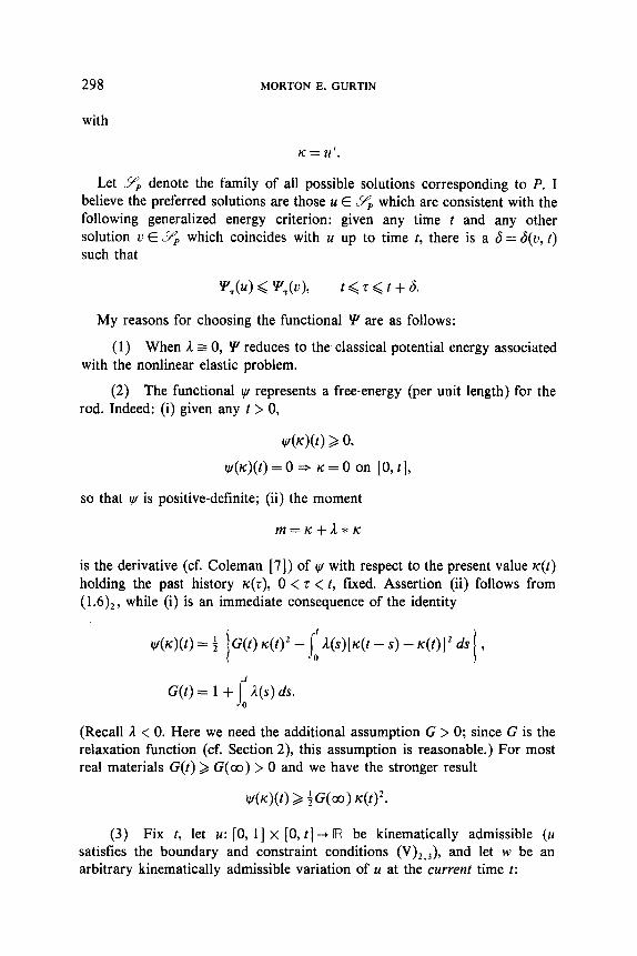
lc= 24’.

Let <YP denote the family of all possible solutions corresponding to P. I believe the preferred solutions are those u E YP which are consistent with the following generalized energy criterion: given any time t and any other solution u E YP which coincides with u up to time t, there is a 6 = 6(v, t) such that

My reasons for choosing the functional Y are as follows:

(1) When 1 z 0, Y reduces to the classical potential energy associated with the nonlinear elastic problem.

(2) The functional ly represents a free-energy (per unit length) for the rod. Indeed: (i) given any t > 0,

&c)(t) = 0 3 K = 0 on [0, t],

so that v/ is positive-definite; (ii) the moment

is the derivative (cf. Coleman [7]) of w with respect to the present value x(t) holding the past history rc(r), 0 < r < t, fixed. Assertion (ii) follows from (1.6)*, while (i) is an immediate consequence of the identity

&c)(t) = 4 I G(t) rC(t)2 -I,; I(s)[fc(t - s) - K(t)12 ds 1 ,

G(t) = 1 + J’~(s) ds. 0

(Recall ,4 < 0. Here we need the additional assumption G > 0; since G is the relaxation function (cf. Section 2), this assumption is reasonable.) For most real materials G(t) > G(co) > 0 and we have the stronger result

(3) Fix t, let u: [0, I] x [0, t] -+ IR be kinematically admissible (U satisfies the boundary and constraint conditions (V),,,), and let w be an arbitrary kinematically admissible variation of ZJ at the current time t:


w(x, 5) = 0 for r < t

= an arbitrary kinematically admissible function of x at r = t.

Then

f YJt(z.4 + EW)la=o = 0

for all such variations w if and only if u satisfies the differential equation (V), at time t. (Note that 1 * K = 1 * (K + EW’) at time t, since K and K + EW'

differ only on a set of measure zero.)

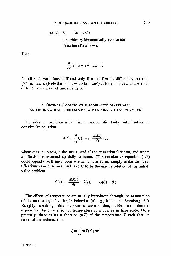
2. OPTIMAL COOLING OF VISCOELASTIC MATERIALS: AN OPTIMIZATION PROBLEM WITH A NONCONVEX COST FUNCTION

Consider a one-dimensioal linear viscoelastic body with isothermal constitutive equation

W) u(t) = I,’ G(t - s) ds ds,

where u is the stress, E the strain, and G the relaxation function, and where all fields are assumed spatially constant. (The consitutive equation (1.2) could equally well have been written in this form: simply make the iden- tifications m c) o, U’ c) E, and take G to be the unique solution of the initial- value problem

G'(s)=?=@), G(O) = P-1

The effects of temperature are usually introduced through the assumption of thermorheologically simple behavior (cf. e.g., Muki and Sternberg [8]). Roughly speaking, this hypothesis asserts that, aside from thermal expansion, the only effect of temperature is a change in time scale. More precisely, there exists a function q(T) of the temperature T such that, in terms of the reduced time

505/48/Z-10


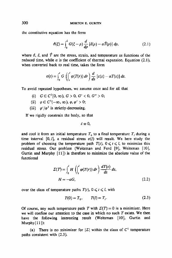
the constitutive equation has the form

where 8, & and ? are the stress, strain, and temperature as functions of the reduced time, while a is the coefftcient of thermal expansion. Equation (2.1), when converted back to real time. takes the form

a(t) = j-’ G (I’q(T(r)) dr) $ [E(S) - LIT(S)] ds. 0 s

To avoid repeated hypotheses, we assume once and for all that

(i) GE C’[O, co), G > 0, G’ < 0, G” > 0; (ii) (p E C3(-co, co), 9, p’ > 0; (iii) cp’/$ is strictly-decreasing.

If we rigidly constrain the body, so that

and cool it from an initial temperature To to a final temperature T, during a time interval [0, I], a residual stress o(l) will result. We here study the problem of choosing the temperature path T(t), 0 < t < I, to minimize this residual stress. Our problem (Weitsman and Ford [9], Weitsman [lo], Gurtin and Murphy [ 111) is therefore to minimize the absolute value of the functional

Z(T) = f H (f q(T(r)) dr ) F ds, 0 s

H = -aG, P-2)

over the class of temperature paths T(f), 0 < t < 1, with

T(O) = To, T(1) = T, . (2.3)

Of course, any such temperature path T with Z(T) = 0 is a minimizer. Here we will confine our attention to the case in which no such T exists. We then have the following interesting result (Weitsman [lo], Gurtin and Murphy[ 111):

(a) There is no minimizer for ]Z] within the class of C’ temperature paths consistent with (2.3).


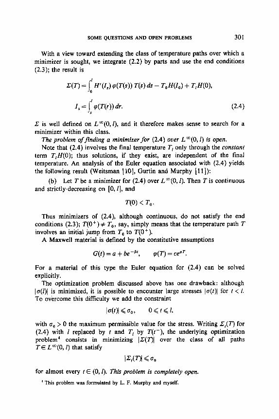
With a view toward extending the class of temperature paths over which a minimizer is sought, we integrate (2.2) by parts and use the end conditions (2.3); the result is

Z’(T) = /‘H’(I,) (p(T(s)) T(s) ds - T,W,) + T,W), 0

I, = I’ q(T(r)) dr. (2.4)

,?Z is well defined on Lm(O, 1), and it therefore makes sense to search for a minimizer within this class.

The problem of finding a minimizer for (2.4) over L”(0, 1) is open. Note that (2.4) involves the final temperature T, only through the constant

term T,Z-Z(O); thus solutions, if they exist, are independent of the final temperature. An analysis of the Euler equation associated with (2.4) yields the following result (Weitsman [lo], Gurtin and Murphy [ 111):

(b) Let T be a minimizer for (2.4) over L”O(0, I). Then T is continuous and strictly-decreasing on [0, I], and

T(0) < To.

Thus minimizers of (2.4), although continuous, do not satisfy the end conditions (2.3); T(0 + ) # To, say, simply means that the temperature path T involves an initial jump from To to T(O+).

A Maxwell material is defined by the constitutive assumptions

G(t) = a + bePB’, p(T) = cepT.

For a material of this type the Euler equation for (2.4) can be solved explicitly.

The optimization problem discussed above has one drawback: although lo(l)1 is minimized, it is possible to encounter large stresses la(t)] for t < 1. To overcome this difficulty we add the constraint

l4Ol G “09 ogt<1,

with co > 0 the maximum permissible value for the stress. Writing C,(T) for (2.4) with I replaced by c and T, by T(t-), the underlying optimization problem4 consists in minimizing [C(r)] over the class of all paths T E L “3(0, 1) that satisfy

Iw-9l G Qo for almost every t E (0, I). This problem is completely open.

4 This problem was formulated by L. F. Murphy and myself.


3. DISPERSAL OF AGE-STRUCTURED POPULATIONS

A. The General Problem

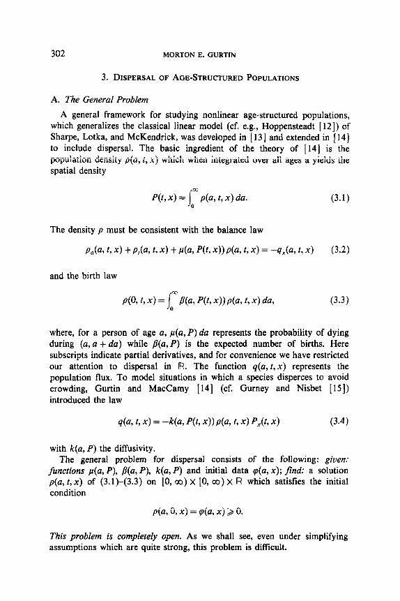
A general framework for studying nonlinear age-structured populations, which generalizes the classical linear model (cf. e.g., Hoppensteadt [ 121) of Sharpe, Lotka, and McKendrick, was developed in [ 131 and extended in ] 141 to include dispersal. The basic ingredient of the theory of [ 141 is the population density p(a, t, x) which when integrated over all ages a yields the spatial density

P(t, x) = Jo* p(a, t, x) da. (3.1)

The density p must be consistent with the balance law

po(a, t, x) + p,(a, t, x) + P(a, W, 4) da, 6 xl = -qx(a,t, x> (3.2)

and the birth law

~(0, t, x) = (* P(a, W, x)) p(a, t, x) da, (3.3) 0

where, for a person of age a, p(a, P) da represents the probability of dying during (a, a + da) while p(a, P) is the expected number of births. Here subscripts indicate partial derivatives, and for convenience we have restricted our attention to dispersal in IF?. The function q(a, t, x) represents the population flux. To model situations in which a species disperces to avoid crowding, Gurtin and MacCamy [ 141 (cf. Gurney and Nisbet [ 151) introduced the law

da, 4 x) = +a, P(t, x)) da, t, 4 P,(t, x) (3.4)

with k(a, P) the diffusivity. The general problem for dispersal consists of the following: given:

functions p(a, P), /3(a, P), k(a, P) and initial data cp(a, x); find: a solution p(a, 1, x) of (3.1)-(3.3) on [0, co) x [0, co) x R which satisfies the initial condition

h-4 0, x) = p(a, x) > 0.

This problem is completely open. As we shall see, even under simplifying assumptions which are quite strong, this problem is difficult.


B. Reduction to Partial Dlzerential Equations

System (3.1)-(3.4) reduces to a pair of partial differential equations when

da9 9 = P(P), p(a, P) = p,(P) eena, k(a, P) = constant. (3.5)

The assumption that ,U be independent of age models a harsh environment in which old age is not a significant cause of death. The literal interpretation of (3.5),, that an individual is most fertile at age zero, is, of course, unreasonable (cf. (3.13)); (3.5), approximately characterizes a population in which individuals are fertile at a relatively young age.

The partial differential equations implied by (3.5) are (Gurtin and MacCamy [ 171)

P, + /J(P) P - PoV') G = W'xL

G, + [P(P) + a - Po(P)I G = (GPxL

where G(t, x) is the auxiliary function

G(t, x) = jam e -aap(a, t, x) da,

(3.6)

(3.7)

and where without loss in generality we have set k = 1. Note that for ,U and &, zero, (3.6), reduces to a degenerate parabolic equation used to study flow through porous media (cf. e.g., Aronson [ 18, 191). On the other hand, for P known (3.6), is first-order, linear, and hyperbolic.

The derivation (Gurtin and MacCamy [13, 16, 201) of (3.6) is not difftcult. To derive (3.6), we integrate (3.2) with respect to a from 0 to co, assume that p(a, t, x)+ 0 as a-+ co, and use (3.1), (3.3), (3.4), and (3.5). Similarly (3.6), is arrived at by multiplying (3.2) by ePao and integrating with respect to a.

The initial conditions corresponding to (3.6) have the form

fv-4 x) = PO(X), G(O, x> = G,(x) (3.8)

with

PO(x) = lom v(a, x) da, G(x) = lam e -aoq(a, x) da. (3.9)

Clearly,

G,(x) = P,,(x) = 0 or 0 < G,(x) < PO(x). (3.10)

304 MORTON E.GURTIN

Conversely, if (3.10) is satisfied, then there exists a continuous initial distribution ~(a, x) such that (3.9) holds.

The initial-value problem (3.6), (3.8) is open.5 This problem is most interesting when the initial data have compact support, as equation (3.6), is degenerate at P = 0. Because of his degeneracy one expects the initially populated region (consisting of the support of P,) to propagate with finite speed.

Assume that PO and G, are bounded, Lipschitz continuous, and consistent with (3.10), and that ,u > 0 and PO > 0 are continuous. Under these assumptions MacCamy and I offer the following conjectures?

(1) There exists a unique weak solution for all time. (2) If P, and (hence) G, have compact support, then P(t, x) and

G(t, x), as functions of x, have compact support in IR for each t > 0, and the supports of P and G coincide.

(3) If

P, > 0 on (x1,x2), P, = 0 otherwise,

with (xi, x2) a bounded open interval, then the set

(3.11)

{(t, 4: m x) > 0)

is bounded by the interval [xi, xz ] of the x-axis, a continuous monotone non- increasing curve x = C(t) with c,(O) = xi, and a continuous monotone nondecreasing curve x = r*(t) with t;,(O) = x2.

(4) If, in addition to (3.1 l), p and &, are constants, then for & > lu + a the “wave fronts” cl(t) and C*(t) tend to -co and +co, respectively, as t -+ co, so that all of R is ultimately populated, while for /I, < p + a the wave fronts have finite limits, so that only a finite interval of lR is ultimately populated.

In solving (3.6) it might be easier to work with the ratio

then (3.6) take the form

P, + 149 P - P,(P) QP = W’,), 3

0 = VW”) - al Q -P,(P) Q*v (3.12)

’ The corresponding problem on an interval [0, I] with boundary conditions P(t, 0) = P(t, I) = 0 has been solved by MacCamy [ 171.

6 Based on results of Oleinik et al. [21], Oleinik [22], Aronson [ 18, 191, Kalashnikov 1231, Knerr 1241, and Gurtin and MacCamy [ 141.


with

Q=Q,-KQ,

the “derivative along characteristics.” When /l,,(P) = constant, (3.12), has a particularly simple form and can, in fact, be integrated explicitly along characteristics. Note that, for /3,, constant, G is proportional to the birth-rate B, while Q is proportional to the per-capita birth-rate B/P.

In place of (3.5),,, one can work with the more general birth function (Gurtin and MacCamy [20])

P(a, P) = e-“” i PL(P) uk k=O

and a diffusivity k(P) which depends on P. In this case, defining

rpV’> = j- WP) dp, W) = J W) @,

b(P) = [PoP’), P,(PL P,vWI,

. . . . . . . . . . . .

(3.13)

Gk(t, X) = jow ake-aap(U, t, x) da,

the general system (3.1~(3.3) reduces to the following system of N + 2 partial differential equations:

Pt + P(P) P - b(P) g = cp(PL

gt + [cl(P) + al g - M(P) g = WWxlx.

I conjecture that the qualitative behavior of this system is no different from that of (3.6).

306 MORTON E.GURTIN

4. POPULATION MODELS THAT ARE PERTURBATIONS OF CHAOTIC SYSTEMS

A. Two Models Based on Easterlin’s Hypothesis

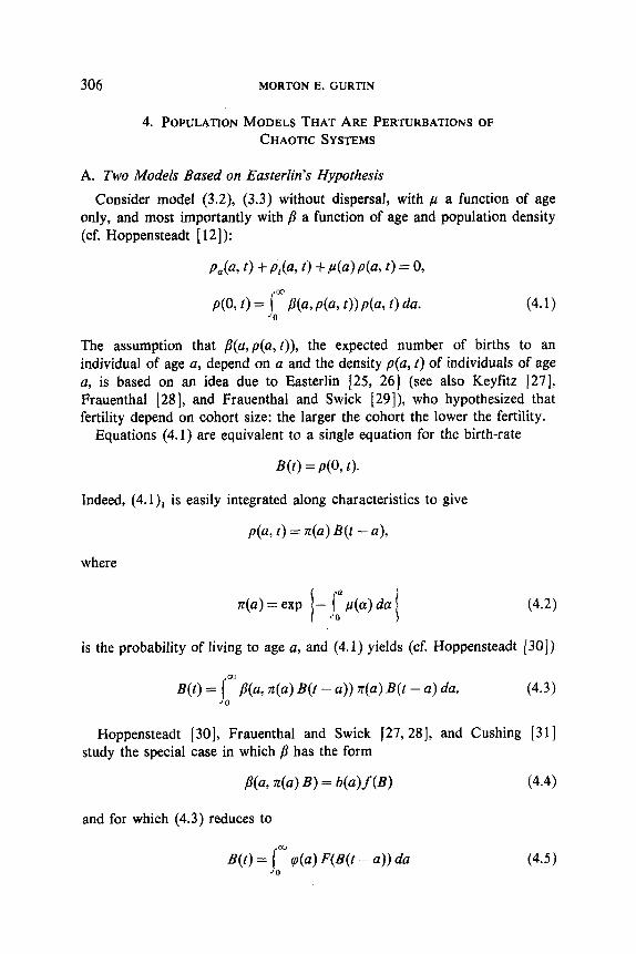
Consider model (3.2), (3.3) without dispersal, with ,u a function of age only, and most importantly with /? a function of age and population density (cf. Hoppensteadt [ 121):

Pata, t> + &(a, 4 + k4a>p(a, t) = 0,

PP, 1) = j@ P(a, da, 0) p(a, t> da. 0

(4.1)

The assumption that P(a,p(a, t)), the expected number of births to an individual of age a, depend on a and the density p(a, t) of individuals of age a, is based on an idea due to Easterlin [25, 261 (see also Keyfitz [27], Frauenthal [28], and Frauenthal and Swick [29]), who hypothesized that fertility depend on cohort size: the larger the cohort the lower the fertility.

Equations (4.1) are equivalent to a single equation for the birth-rate

Indeed, (4.1), is easily integrated along characteristics to give

p(a, f> = XL(a) W - a>,

where

is the probability of living to age a, and (4.1) yields (cf. Hoppensteadt (301)

B(t) = jm P(a, n(a) B(t - a)) n(a) B(t - a) da. (4.3) 0

Hoppensteadt [30], Frauenthal and Swick 127,281, and Cushing [3 11 study the special case in which /I has the form

(4.4)

and for which (4.3) reduces to

B(t) = jm q(a) F(B(t - a)) da 0

(4.5)


with

F@) = wv), da> = b(a) 4a).

Assume, without loss in generality, that b in (4.4) is normalized to insure’

I 00

p(u) da = 1, 0

and consider, for the moment, the rather restrictive assumption

p(u) = &a - h)

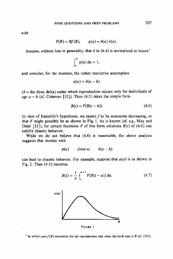
(6 = the dirac delta) under which reproduction occurs only for individuals of age a = h (cf. Coleman [32]). Then (4.5) takes the simple form

B(t) = F(B(t - h)). (4.6)

In view of Easterlin’s hypothesis, we expect f to be monotone decreasing, so that F might possibly be as shown in Fig. 1. As is known (cf. e.g., May and Oster [33]), for certain functions F of this form solutions B(t) of (4.6) can exhibit chaotic behavior.

While we do not believe that (4.6) is reasonable, the above analysis suggests that models with

close to &a - h)

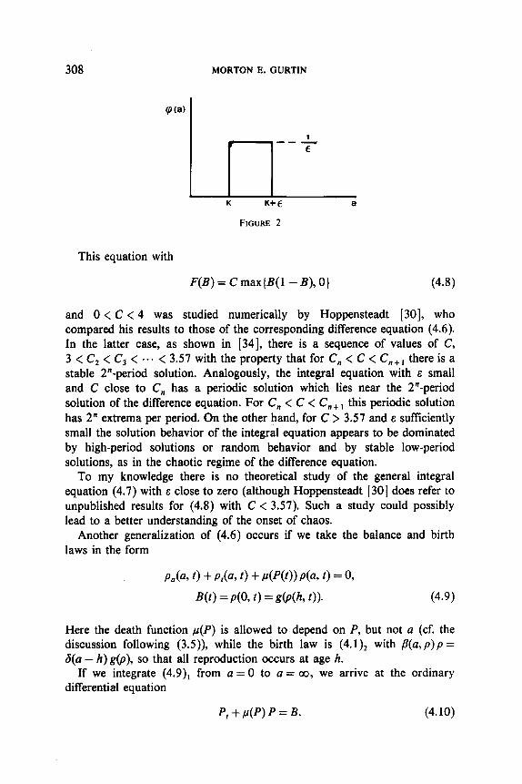
can lead to chaotic behavior. For example, suppose that o(u) is as shown in Fig. 2. Then (4.5) becomes

F(B(t - a)) da.

F(B)

FIGURE 1

(4.7)

’ In which case/(E) represents the net reproduction rate when the birth-rate is B (cf. [ 29 1).


rp(a)

1 t ---

E

K K+E a

FIGURE 2

This equation with

F(B) = C max{B(l -B), 0} (4.8)

and 0 < C < 4 was studied numerically by Hoppensteadt [30], who compared his results to those of the corresponding difference equation (4.6). In the latter case, as shown in [34], there is a sequence of values of C, 3<C*<Cj<“* < 3.57 with the property that for C, < C < C,, I there is a stable 2”-period solution. Analogously, the integral equation with E small and C close to C, has a periodic solution which lies near the 2”-period solution of the difference equation. For C, < C < C, + i this periodic solution has 2” extrema per period. On the other hand, for C > 3.57 and E sufficiently small the solution behavior of the integral equation appears to be dominated by high-period solutions or random behavior and by stable low-period solutions, as in the chaotic regime of the difference equation.

To my knowledge there is no theoretical study of the general integral equation (4.7) with E close to zero (although Hoppensteadt [30] does refer to unpublished results for (4.8) with C < 3.57). Such a study could possibly lead to a better understanding of the onset of chaos.

Another generalization of (4.6) occurs if we take the balance and birth laws in the form

Pa@, 0 + P,(4 0 + W(t)) de t) = 0,

W) = do, 0 = da 0). (4.9)

Here the death function p(P) is allowed to depend on P, but not a (cf. the discussion following (3.5)), while the birth law is (4.1), with fi(a, p)p = &a - h) g@), so that all reproduction occurs at age h.

If we integrate (4.9), from u = 0 to a = co, we arrive at the ordinary differential equation

P,+p(P)P=B. (4.10)


To derive a second equation relating P and B we integrate (4.9), along characteristics; the result is

p(a, t) = B(t - a) exp

which with (4.9), yields

I -I’ p(P@))dJ .

I-h I) (4.11)

The problem reduces to solving (4. lo), (4.11). Since crowding should increase the death-rate, we expect p(P) to be an

increasing function of P. In particular, for

olo, & > 0) P(P) = PO + EP

system (4. lo), (4.11) reduces to

B(t) = F

with

P,+poP+cP2=B,

F(z) = g(e-“O”z).

(4.12)

Note that for E = 0, (4.12), reduces to the difference equation (4.6); thus for E small we again have a perturbation of a possibly chaotic model. At present there are neither numerical nor theoretical results for the perturbed model.

B. A Model with Dl@uusion

As our last model we consider the balance law (4.1), , but with one- dimensional random dispersal

P&P 6 x) + P,@, t, x> + cl(a) P(U, t, x) = EPxx(U, 6 x),

where E > 0 is constant. For the associated birth law we use (4.9),:

B(t, x) = ~(0, c, x) = g@(h, 6 4). (4.13)

We consider these equations on a finite interval 0 < x Q 1 with boundary conditions “p or px equal to zero” at each endpoint, or on an infinite interval with p-+ 0 sufficiently fast. Let S, denote the evolution operator for the

310 MORTON E.GURTIN

equation u, = EU,, with the above boundary or regularity conditions: for sufficiently smooth initial data u,(x) the solution u(x, t) is given by

u(*, t) = s,u,.

Let

p(a, t, x) = z(a) &4 6 x> with 71 given by (4.2). Then

ra+r~=~tl,,~

or

& <(u + 7, t + 7, x) = Et&2 t 7, t t 7, xl,

and

Thus, by (4.14),

@a t 7, t + 7, *> = s&2, t, a).

P@, 4 *) = n(h) s/J@, t - h, *)

and (4.13) yields

with

B(t, *) = F(S,B(t - h, a))

(4.14)

(4.15)

F(z) = g@(h) z)* For certain functions F with qualitative behavior of the type indicated in

Fig. 1 and for E sufficiently small, I expect solutions of (4.15) to exhibit chaotic behavior. It would be interesting to see the effects of diffusion on this behavior: What happens as E is slowly increased? Can random diffusion overwhelm this chaotic behavior (if it exists)?

ACKNOWLEDGMENTS

This work was supported by the Army Research Offlice and by the National Science Foun- dation. The author is grateful to C. Baiocchi, L. Murphy, D. Reynolds, and K. Spear for valuable comments.

SOMEQUESTIONS AND OPEN PROBLEMS 311

REFERENCES

1. D. W. REYNOLDS, On the buckling of viscoelastic rods, in preparation. 2. A. E. H. LOVE, “A Treatise on the Mathematical Theory of Elasticity,” Fourth ed.,

Dover, New York, 1944. 3. J. N. DIST~FANO, Sulla stabilita in regime viscoelastico a comportamento lineare, I, Atti

Accad. Naz. Lincei Rend. Cl. Sci. Fis. Mat. Natur (8) 21 (1960), 356-361. 4. J. N. DISTBFANO, Creep buckling of slender columns, J. Strut. Div. Proc. ASCE 91

(1965), 127-150. 5. M. E. GURTIN, V. J. MIZEL, AND D. W. REYNOLDS, On nontrivial solutions for a

compressed linear viscoelastic rod, J. Appl. Mech. 49 (1982), 245-246. 6. E. L. REISS, Column buckling-An elementary example of bifurcation, in “Bifurcation

Theory and Nonlinear Eigenvalue Problems” (J. B. Keller and S. Antman, Eds.), Benjamin, New York, 1969.

7. B. D. COLEMAN, Thermodynamics of materials with memory, Arch. Rational Mech. Anal. 17 (1964), l-46.

8. R. MUKI AND E. STERNBERG, On transient thermal stresses in viscoelastic materials with temperature-dependent properties, J. Appl. Mech. 83 (196 1), 193-207.

9. Y. WEITSMAN AND D. FORD, On the optimization of cool-down temperatures in viscoelastic resins, Proc. Sot. Engrg. Sci. (1977).

10. Y. WEITSMAN, Optimal cool-down in linear viscoelasticity, J. Appl. Mech. 47 (1980), 35-39.

11. M. E. GURTIN AND L. F. MURPHY, On optimal temperature paths for thermorheologically simple viscoelastic materials, Quart. Appl. Math. 38 (1980), 179-189.

12. F. HOPPENSTEADT, “Mathematical Theories of Populations: Demographics, Genetics and Epidemics,” SIAM, Philadelphia, 1975.

13. M. E. GURTIN AND R. C. MACCAMY, Non-linear age-dependent population dynamics, Arch. Rational Mech. Anal. 54 (1974), 281-300.

14. M. E. GURTIN AND R. C. MACCAMY, On the diffusion of biological populations, Math. Biosci. 33 (1977), 35-49.

15. W. S. C. GURNEY AND R. M. NISBET, The regulation of inhomogeneous populations, J. Theoret. Biol. 52 (1975), 441-457.

16. M. E. GURTIN AND R. C. MACCAMY, Diffusion models for age-structured populations, Math. Biosci. 54 (1981), 49-59.

17. R. C. MACCAMY, A population model tiith nonlinear diffusion. J. Drfirential Equations 39 (1981), 52-72.

18. D. G. ARONSON, Regularity properties of flows through porous media, SIAM J. Appl. Math. 17 (1969), 461467.

19. D. G. ARONSON, Regularity properties of flows through porous media: The interface, Arch. Rational Mech. Anal. 37 (1970), l-10.

20. M. E. GURTIN AND R. C. MACCAMY, Some simple models for nonlinear age-dependent population dynamics, Math. Biosci. 43 (1979), 199-211.

21. 0. A. OLEINIK, A. S. KALASHNIKOV, AND CHU YUI-LIN’, The Cauchy problem and boundary problems for equations of the type of nonstationary filtration, Izu. Akad. Nauk SSSR Ser. Mat. 22 (1958), 667-704.

22. 0. A. OLEINIK, On some degenerate quasilinear equations, Istituto Nazionale di Alta Mathematics Seminari 1962-1963, Cremonese, Rome, 1965.

23. A. S. KALASHNIKOV, On the occurrence of singularities in the solutions of the equation of nonstationary filtration, Zh. Vychisl. Mat. i Mat. Fir. 7 (1967), 440-444.

24. B. F. KNERR, “Some Results Concerning Solutions of the Cauchy Problem for the Porous


Medium Equation When the Initial Data Have Compact Support,” Ph.D. dissertation, Northwestern University, 1976.

25. R. A. EASTERLIN, The baby boom in perspective, Amer. Econom. Rev. 51 (1961). 869-911.

26. R. A. EASTERLIN, The current fertility decline and projected fertility changes, in “Population, Labor Force, and Long Swings in Economic Growth: The American Experience,” Chap. 5, Columbia Univ. Press, New York, 1968.

27. N. KEYFITZ, Population waves, in “Population Dynamics” (T. N. E. Greville, Ed.), Academic Press, New York, 1972.

28. J. C. FRAUENTHAL, A dynamic model for human population growth, Theoret. Populafion Biol. 8 (1975), 64-73.

29. J. C. FRAUENTHAL AND K. E. SWICK, Limit cycle oscillations of the human population, forthcoming.

30. F. C. HOPPENSTEADT, A nonlinear renewal equation with periodic and chaotic solutions, SIAM-AMS Proc. 10 (1976), 51-60.

31. J. M. CUSHINO, Model stability and instability in age structured populations, J. Theoret. Biol. 86 (1980), 709-730.

32. B. D. COLEMAN, On the growth of populations with narrow spread in reproductive age. I. General theory and examples, J. Math. Biol. 6 (1978), 1-19.

33. R. MAY AND G. OSTER, Bifurcations and dynamic complexity in simple ecological models, Amer. Nat. 110 (1976), 153-173.

34. F. C. HOPPENSTEADT AND J. M HYMAN, Periodic solutions of a logistic difference equation, SIAM J. Appf. Math., forthcoming.

Prinred in Belgium

some questions and open problems in continuum mechanics ... · journal of differential equations...

Documents