some take-away games on discrete structures
TRANSCRIPT

University of Kentucky University of Kentucky
UKnowledge UKnowledge
Theses and Dissertations--Mathematics Mathematics
2017
Some Take-Away Games on Discrete Structures Some Take-Away Games on Discrete Structures
Kristen M. Barnard University of Kentucky, [email protected] Author ORCID Identifier:
http://orcid.org/0000-0003-4727-0190 Digital Object Identifier: https://doi.org/10.13023/ETD.2017.151
Right click to open a feedback form in a new tab to let us know how this document benefits you. Right click to open a feedback form in a new tab to let us know how this document benefits you.
Recommended Citation Recommended Citation Barnard, Kristen M., "Some Take-Away Games on Discrete Structures" (2017). Theses and Dissertations--Mathematics. 44. https://uknowledge.uky.edu/math_etds/44
This Doctoral Dissertation is brought to you for free and open access by the Mathematics at UKnowledge. It has been accepted for inclusion in Theses and Dissertations--Mathematics by an authorized administrator of UKnowledge. For more information, please contact [email protected].

STUDENT AGREEMENT: STUDENT AGREEMENT:
I represent that my thesis or dissertation and abstract are my original work. Proper attribution
has been given to all outside sources. I understand that I am solely responsible for obtaining
any needed copyright permissions. I have obtained needed written permission statement(s)
from the owner(s) of each third-party copyrighted matter to be included in my work, allowing
electronic distribution (if such use is not permitted by the fair use doctrine) which will be
submitted to UKnowledge as Additional File.
I hereby grant to The University of Kentucky and its agents the irrevocable, non-exclusive, and
royalty-free license to archive and make accessible my work in whole or in part in all forms of
media, now or hereafter known. I agree that the document mentioned above may be made
available immediately for worldwide access unless an embargo applies.
I retain all other ownership rights to the copyright of my work. I also retain the right to use in
future works (such as articles or books) all or part of my work. I understand that I am free to
register the copyright to my work.
REVIEW, APPROVAL AND ACCEPTANCE REVIEW, APPROVAL AND ACCEPTANCE
The document mentioned above has been reviewed and accepted by the student’s advisor, on
behalf of the advisory committee, and by the Director of Graduate Studies (DGS), on behalf of
the program; we verify that this is the final, approved version of the student’s thesis including all
changes required by the advisory committee. The undersigned agree to abide by the statements
above.
Kristen M. Barnard, Student
Dr. Carl W. Lee, Major Professor
Dr. Peter Hislop, Director of Graduate Studies

SOME TAKE-AWAY GAMES ON DISCRETE STRUCTURES
DISSERTATION
A dissertation submitted in partialfulfillment of the requirements forthe degree of Doctor of Philosophyin the College of Arts and Sciences
at the University of Kentucky
ByKristen M. BarnardLexington, Kentucky
Director: Dr. Carl W. Lee, Professor of MathematicsLexington, Kentucky 2017
Copyright c© Kristen M. Barnard 2017

ABSTRACT OF DISSERTATION
SOME TAKE-AWAY GAMES ON DISCRETE STRUCTURES
The game of Subset Take-Away is an impartial combinatorial game posed by DavidGale in 1974. The game can be played on various discrete structures, includingbut not limited to graphs, hypergraphs, polygonal complexes, and partially orderedsets. While a universal winning strategy has yet to be found, results have beenfound in certain cases. In 2003 R. Riehemann focused on Subset Take-Away onbipartite graphs and produced a complete game analysis by studying nim-values. Inthis work, we extend the notion of Take-Away on a bipartite graph to Take-Awayon particular hypergraphs, namely oddly-uniform hypergraphs and evenly-uniformhypergraphs whose vertices satisfy a particular coloring condition. On both structureswe provide a complete game analysis via nim-values. From here, we consider differentdiscrete structures and slight variations of the rules for Take-Away to produce someinteresting results. Under certain conditions, polygonal complexes exhibit a sequenceof nim-values which are unbounded but have a well-behaved pattern. Under otherconditions, the nim-value of a polygonal complex is bounded and predictable basedon information about the complex itself. We introduce a Take-Away variant whichwe call Take-As-Much-As-You-Want, and we show that, again, nim-values can growwithout bound, but fortunately they are very easily described for a given graph basedon the total number of vertices and edges of the graph. Finally we consider Take-Awayon a specific type of partially ordered set which we call a rank-complete poset. Wehave results, again via an analysis of nim-values, for Take-Away on a rank-completeposet for both ordinary play as well as misere play.
KEYWORDS: Take-Away, combinatorial game, misere game, hypergraph, poset,polytopal complex
Author’s signature: Kristen M. Barnard
Date: May 1, 2017

SOME TAKE-AWAY GAMES ON DISCRETE STRUCTURES
ByKristen M. Barnard
Director of Dissertation: Carl W. Lee
Director of Graduate Studies: Dr. Peter Hislop
Date: May 1, 2017
Dedicated to my mother, Debbie, who hated math but loved me beyond measure.I hope I always make you proud.

ACKNOWLEDGMENTS
One thing I always loved about getting a new album, whether it be on cassette, CD,
or vinyl, is reading the artist’s acknowledgments where they took the time to thank
all the people that helped them along the way, from close friends and family to the
companies that made their equipment. This is my moment to do the same.
I cannot thank Dr. Carl Lee enough for all that he has done for me during my
long journey to this point. Thank you, Dr. Lee, for letting me know I belonged,
encouraging me, inspiring me, teaching me, and showing me great kindness and pa-
tience. Thanks for turning your dining room into a workspace, and for the tea and
conversation.
Thank you to my committee members for your willingness to serve. Dr. Margaret
Mohr-Schroeder and Dr. Adib Bagh, thank you for your thoughtful feedback. Dr. Ben
Braun, thank you for all of your support through my journey. Dr. Uwe Nagel, thank
you for your understanding during the hardest semester of my life.
Thank you to Dr. Qiang Ye, Dr. Peter Perry, and Dr. Peter Hislop for your work
as DGS during the time I have been at UK and for helping me to meet the challenges
associated with being a part-time student. Also, a great thanks to the wonderful Mrs.
Sheri Rhine who keeps the department running and has solved many a predicament
for me.
My colleagues, students, and administration at Berea College have been remark-
ably supportive of me all along the way. It has not been easy balancing a full time
career and working on a PhD part-time, and I know that it could not have been done
without your help. Thank you for all you have done, and thank you for believing in
me.
iii

I appreciate all the professors I had at Eastern Kentucky University, particularly
Dr. Kirk Jones. Thank you, Dr. Jones, for constantly asking if I was a math major
yet, teaching me about the math gods, and for all your help in complex analysis and
beyond.
To all of my fellow graduate students, both at EKU and UK: thank you for
teaching me how much better it is to learn with others. Studying for comps and
prelims and working on homework with you made me a better mathematician.
To my math and non-math friends: thank you for being there for all the emotional
support, love, and laughter you have brought my life, and for providing necessary
distractions at just the right times.
Keath, you have been with me through this since day one. When things get too
hard you give me a shoulder to cry on and encouragement to keep going. You give me
hugs and tea. You never stop believing in me, and you won’t let me stop believing
in myself. You are my cheerleader. You have my thanks and my love.
To my paternal grandparents, Delmer and Hazel, thank you for all that you did
for your family. You made sure all your children went to college, and now all of their
children have as well—in fact, there are Master’s Degrees, Specialist Degrees, and
now a PhD. Granny, thank you for teaching me to crochet. G. P., thank you for your
sense of humor and wisdom. I miss you both every day.
To my maternal grandparents, Johnnie and Lorine, thank you for your prayers,
support, and encouragement. I am so lucky to have you in my life. Thank you both
for helping me learn to be a storyteller and for playing games with me. I’m sure you
never thought that Dots-and-Boxes (Mamaw) and Cars-and-Trucks (Papaw) would
have a relationship to my dissertation one day.
Kellyn, thank you for being one of the funniest, smartest, most thoughtful people
I know. Thank you for being you, for growing up into someone I am proud to call
my best friend.
iv

On one of the first days of my first class at UK, Dr. Hislop asked us if we knew
if our favorite mathematician was right- or left-handed. I smiled to myself almost
immediately because I knew the answer: my dad writes with his right hand. My
father, Phil, was my earliest math teacher, my tutor, and my hero. He has been my
test audience, my supporter in uncountable ways, and he loves me unconditionally,
even when I’m pretty unlovable. I have been blessed.
Thank you to my mother, Debbie, for your love and encouragement. Thank you
for teaching me to be strong, and for being strong for me when I couldn’t. I don’t
have words to describe how much I miss you, but thank you for letting me know in
just the right ways and just the right times that you are still with me.
Thank you to all the brilliant, pioneering women mathematicians and scientists
who have come before me. Without you to pave the way my journey might never
have been. I hope that I can be an encouragement to all the students that I teach,
but especially I hope to be a role model for young women in mathematics.
To the members of Bon Jovi, Kings of Leon, the Eagles, the Monkees, and Ryan
Adams . . . your music is the soundtrack to my life, and thus to this dissertation.
Thank you for writing the words and the music that make my heart happy and stir
my soul.
Lastly, this dissertation could not have been possible without lots of pizza, tea,
and chocolate. Thanks also to Qdoba, whose giant burritos are equally wonderful for
celebration or catharsis.
Kristen Barnard uses PaperMate Flair felt-tip pens.
v

TABLE OF CONTENTS
Acknowledgments . . . . . . . . . . . . . . . . . . . . . . . . . . . . . . . . . . iii
Table of Contents . . . . . . . . . . . . . . . . . . . . . . . . . . . . . . . . . . vi
List of Figures . . . . . . . . . . . . . . . . . . . . . . . . . . . . . . . . . . . viii
Chapter 1 Introduction . . . . . . . . . . . . . . . . . . . . . . . . . . . . . . 11.1 What Is A Combinatorial Game? . . . . . . . . . . . . . . . . . . . . 11.2 Nim and Impartial Games . . . . . . . . . . . . . . . . . . . . . . . . 71.3 Poset Take-Away . . . . . . . . . . . . . . . . . . . . . . . . . . . . . 121.4 The Bipartite Graph Game . . . . . . . . . . . . . . . . . . . . . . . 141.5 Polytopal Complexes . . . . . . . . . . . . . . . . . . . . . . . . . . . 171.6 A Dissertation Road Map . . . . . . . . . . . . . . . . . . . . . . . . 18
Chapter 2 Hypergraph Games . . . . . . . . . . . . . . . . . . . . . . . . . . 212.1 Game Description . . . . . . . . . . . . . . . . . . . . . . . . . . . . . 212.2 Oddly Uniform Hypergraphs . . . . . . . . . . . . . . . . . . . . . . . 232.3 Take-Away on Oddly Uniform Hypergraphs . . . . . . . . . . . . . . 262.4 Corollaries and Related Games . . . . . . . . . . . . . . . . . . . . . 282.5 Evenly Uniform Hypergraphs . . . . . . . . . . . . . . . . . . . . . . 302.6 Hypergraph Colorings . . . . . . . . . . . . . . . . . . . . . . . . . . 312.7 Take-Away on Evenly Uniform Hypergraphs . . . . . . . . . . . . . . 362.8 Even Polygonal Complexes . . . . . . . . . . . . . . . . . . . . . . . . 422.9 Hypergraphs With Both Odd And Even Hyperedges . . . . . . . . . . 462.10 Type 1 Take-Away versus Type 2 Take-Away . . . . . . . . . . . . . 53
Chapter 3 Polygon Games . . . . . . . . . . . . . . . . . . . . . . . . . . . . 563.1 Game Play . . . . . . . . . . . . . . . . . . . . . . . . . . . . . . . . . 563.2 Even Polygons with One Tail . . . . . . . . . . . . . . . . . . . . . . 603.3 Even Polygons with Two Tails . . . . . . . . . . . . . . . . . . . . . . 713.4 Even Polygons with Three Tails . . . . . . . . . . . . . . . . . . . . . 893.5 Quadrilaterals with Four Tails . . . . . . . . . . . . . . . . . . . . . . 1003.6 Even Polygons with Tails at Every Vertex . . . . . . . . . . . . . . . 104
Chapter 4 Take-As-Much-As-You-Want . . . . . . . . . . . . . . . . . . . . . 1074.1 Game Play . . . . . . . . . . . . . . . . . . . . . . . . . . . . . . . . . 1074.2 Take-As-Much-As-You-Want on a Graph . . . . . . . . . . . . . . . . 1074.3 Take-As-Much-As-You-Want on a Polytopal Complex . . . . . . . . . 111
Chapter 5 Poset Games . . . . . . . . . . . . . . . . . . . . . . . . . . . . . 1165.1 Take-Away on a Rank-Complete Poset . . . . . . . . . . . . . . . . . 118
vi

5.2 Misere Take-Away on a Rank-Complete Poset . . . . . . . . . . . . . 1225.3 Misere Take-Away on the Sum of Rank-Complete Posets . . . . . . . 127
Chapter 6 Areas for Further Research . . . . . . . . . . . . . . . . . . . . . . 133
Bibliography . . . . . . . . . . . . . . . . . . . . . . . . . . . . . . . . . . . . 136
Vita . . . . . . . . . . . . . . . . . . . . . . . . . . . . . . . . . . . . . . . . . 137
vii

LIST OF FIGURES
2.1 A hypergraph with hyperedges {A,B}, {A,C}, {B,C},{B,D}, {C,D},{A,B,C}, and {A,B,C,D}. . . . . . . . . . . . . . . . . . . . . . . . . . 22
2.2 An oddly uniform hypergraph with hyperedges {E,F, J,K, L} and {E, J,K}. 242.3 A tetrahedron. . . . . . . . . . . . . . . . . . . . . . . . . . . . . . . . . 292.4 A polygonal complex consisting of triangles without edges. . . . . . . . . 302.5 An evenly uniform hypergraph with a standard coloring. . . . . . . . . . 322.6 An evenly uniform hypergraph with a marked coloring. . . . . . . . . . . 332.7 Another evenly uniform hypergraph with a marked coloring. . . . . . . . 332.8 A hypergraph that does not have a marked coloring. . . . . . . . . . . . 342.9 A finite polygonal complex. . . . . . . . . . . . . . . . . . . . . . . . . . 412.10 A finite polygonal complex divided into quadrilaterals and with a marked
coloring. . . . . . . . . . . . . . . . . . . . . . . . . . . . . . . . . . . . . 412.11 A finite polygonal complex comprised of hexagons. . . . . . . . . . . . . 422.12 A finite polygonal complex comprised of squares. . . . . . . . . . . . . . 422.13 A finite polygonal complex comprised of octagons and squares. . . . . . . 432.14 Schlegel diagrams of positions obtained from the truncated tetrahedron
that have nim-value 0. . . . . . . . . . . . . . . . . . . . . . . . . . . . . 472.15 Schlegel diagrams of positions obtained from the truncated tetrahedron
that have nim-value 1. . . . . . . . . . . . . . . . . . . . . . . . . . . . . 482.16 Schlegel diagrams of positions obtained from the truncated tetrahedron
that have nim-value 2. . . . . . . . . . . . . . . . . . . . . . . . . . . . . 482.17 Schlegel diagrams of positions obtained from the truncated tetrahedron
that have nim-value 3. . . . . . . . . . . . . . . . . . . . . . . . . . . . . 492.18 Schlegel diagrams of positions obtained from the truncated tetrahedron
that have nim-value 4. . . . . . . . . . . . . . . . . . . . . . . . . . . . . 492.19 Schlegel diagrams of positions obtained from the truncated tetrahedron
that have nim-value 6. . . . . . . . . . . . . . . . . . . . . . . . . . . . . 502.20 Schlegel diagram of a truncated tetrahedron showing a marked coloring. . 502.21 A table with observed data about truncated tetrahedron game positions
with different nim-values. . . . . . . . . . . . . . . . . . . . . . . . . . . 512.22 A hexagon with its edges. . . . . . . . . . . . . . . . . . . . . . . . . . . 53
3.1 A portion of a square grid. . . . . . . . . . . . . . . . . . . . . . . . . . . 573.2 A portion of a square grid with even degree corner vertices. . . . . . . . . 573.3 A square with a single tail. . . . . . . . . . . . . . . . . . . . . . . . . . . 613.4 A square with two tails. . . . . . . . . . . . . . . . . . . . . . . . . . . . 613.5 A table showing some nim-values for an even polygon with one tail (row
1), two tails with one having fixed length 1 (row 2), and two tails withone having fixed length 2 (row 3). . . . . . . . . . . . . . . . . . . . . . . 62
3.6 An even polygon with tails connected to each of three vertices. . . . . . . 89
viii

3.7 A table showing the nim-values for an even polygon with three tails, onehaving fixed length 0. . . . . . . . . . . . . . . . . . . . . . . . . . . . . . 90
3.8 A table showing the nim-values for an even polygon with three tails, onehaving fixed length 1. . . . . . . . . . . . . . . . . . . . . . . . . . . . . . 91
3.9 A table showing the nim-values for an even polygon with three tails, onehaving fixed length 2. . . . . . . . . . . . . . . . . . . . . . . . . . . . . . 91
3.10 A table showing the nim-values for an even polygon with three tails, onehaving fixed length 3. . . . . . . . . . . . . . . . . . . . . . . . . . . . . . 92
3.11 A table showing the nim-values for an even polygon with three tails, onehaving fixed length 4. . . . . . . . . . . . . . . . . . . . . . . . . . . . . . 92
3.12 A table showing the nim-values for an even polygon with three tails, onehaving fixed length 5. . . . . . . . . . . . . . . . . . . . . . . . . . . . . . 93
3.13 A table showing the nim-values for an even polygon with three tails, onehaving fixed length 6. . . . . . . . . . . . . . . . . . . . . . . . . . . . . . 93
3.14 A table showing the nim-values for an even polygon with three tails, onehaving fixed length 7. . . . . . . . . . . . . . . . . . . . . . . . . . . . . . 94
3.15 A table showing the nim-values for an even polygon with three tails, onehaving fixed length 8. . . . . . . . . . . . . . . . . . . . . . . . . . . . . . 94
3.16 A table showing the nim-values for an even polygon with three tails, onehaving fixed length 9. . . . . . . . . . . . . . . . . . . . . . . . . . . . . . 95
3.17 A table showing the nim-values for an even polygon with three tails, onehaving fixed length 10. . . . . . . . . . . . . . . . . . . . . . . . . . . . . 95
3.18 A table showing the nim-values for an even polygon with three tails, onehaving fixed length 11. . . . . . . . . . . . . . . . . . . . . . . . . . . . . 96
3.19 A table showing the nim-values for an even polygon with three tails, onehaving fixed length 12. . . . . . . . . . . . . . . . . . . . . . . . . . . . . 96
3.20 A table showing the nim-values for an even polygon with three tails, onehaving fixed length 13. . . . . . . . . . . . . . . . . . . . . . . . . . . . . 97
3.21 A table showing the nim-values for an even polygon with three tails, onehaving fixed length 14. . . . . . . . . . . . . . . . . . . . . . . . . . . . . 97
3.22 A table showing the nim-values for an even polygon with three tails, onehaving fixed length 15. . . . . . . . . . . . . . . . . . . . . . . . . . . . . 98
3.23 A table showing the nim-values for an even polygon with three tails, onehaving fixed length 16. . . . . . . . . . . . . . . . . . . . . . . . . . . . . 98
3.24 A table showing the nim-values for an even polygon with three tails, onehaving fixed length 17. . . . . . . . . . . . . . . . . . . . . . . . . . . . . 99
3.25 A quadrilateral with a tail connected to every vertex. . . . . . . . . . . . 1003.26 A quadrilateral with a tail connected to every vertex and all the moves
that can be made from that position in a game of Type 2 Take-Away. Thenim-value of each position is also included. . . . . . . . . . . . . . . . . . 100
5.1 The Hasse diagram of a rank-complete poset. . . . . . . . . . . . . . . . 1195.2 Possible positions after one move in Take-Away played on Figure 5.1 . . 1195.3 The Hasse diagram of a rank-complete poset with an extra element, t,
appended beneath the rank 0 elements. . . . . . . . . . . . . . . . . . . . 122
ix

Chapter 1 Introduction
With respect to the creation and completion of this dissertation, two very impor-
tant things happened in 1982: I was born, and Elwyn Berlekamp, John Conway,
and Richard Guy published the first volume of their series Winning Ways For Your
Mathematical Plays. In this first chapter we will reference this text and other works
to introduce the fundamentals of combinatorial game theory, and impartial games in
particular.
1.1 What Is A Combinatorial Game?
In this section we will begin to outline the basics of combinatorial game theory.
There are several conditions associated with combinatorial games:
• Combinatorial games are two-player games, say player A and player B, and the
players move alternately.
• Combinatorial games are games of complete information; that is, the rules of
the game are clearly defined and at any given point in the game—henceforth
known as a position of the game—both players know the current position and
all of the possible moves that can be made from that position.
• Combinatorial games involve no elements of chance such as spinners, dice, draw-
ing or dealing cards, et cetera.
1

• Alternating play continues between the players until one player is unable to
move per the rules of the game, and the rules of the game are such that the
game will end after a finite number of moves.
• The convention of normal play is that if a player makes the final possible move
of the game then she is the winner. Alternatively, if the rules are such that the
player who makes the last possible move of the game is declared the loser then
we call this misere play. In particular, no ties are permitted [3].
The games in this dissertation will follow all of these conditions, but it is impor-
tant to note that combinatorial game theory techniques can also be used to study
some games where some of the conditions are relaxed. The conditions which must
hold, though, are the condition of complete information and the condition of having
no elements of chance involved. In order to determine a winning strategy for a com-
binatorial game, it is important to know what positions are options after each move.
Further, of the games we discuss in this work, most are played under normal play;
however we do investigate some misere games in Chapter 5.
Of course, the goal of studying combinatorial games is to determine a winning
strategy for them. A winning strategy for player A (respectively, B) in a combinatorial
game is a strategy that specifies a move from each position that guarantees a win for
player A (respectively, B) [1].
One possible way to search for a winning strategy is a brute force method enu-
merating every possible game scenario. It is not hard to see that as the size of the
game grows this task also grows, and could soon become unmanageable and likely
2
very tedious. Also, doing this forces us to examine games in which players make
moves that we recognize as mistakes—think, for example, of instances where a player
makes a move that fails to block a 3-in-a-row in Tic-Tac-Toe. Thinking of the brute
force method just described and that these mistakes must be taken into account, we
see that there are scenarios in which player A could win as well as scenarios in which
player B could win, and this does not efficiently lead to describing a winning strategy.
To study combinatorial games in search of a winning strategy more efficiently, we
must assume that both players play perfectly [1]. Playing perfectly means that, since
both players know the rules of the game and have complete information available to
them, if a player knows that she can make a move that will force her opponent to
lose the game then she must make that move. If no such move is available, playing
perfectly is just making a legal move in the game.
With this assumption of perfect play, studying the game strategies becomes much
more interesting and, in some cases, more straightforward. We will assume, of course,
that both players are playing perfectly in the games studied in this dissertation. With
the assumption, we have that one of the players, either player A or player B, will have
a guaranteed winning strategy in a game, but not both. This is the Fundamental
Theorem of Combinatorial Games.
Theorem 1.1 (Fundamental Theorem of Combinatorial Games). Let G be a com-
binatorial game, played between two players A and B, with player A moving first.
Then either a winning strategy in G exists for player A or a winning strategy exists
for player B, but not both.
3

This is a standard result, and proofs can be found in most references on combina-
torial games [8, 1]. It is important to note that Theorem 1.1 guarantees that there will
be a winner, but it does not provide any details about the winning strategy or how
to determine the winner. Determining who has the winning strategy and describing
it is the focus of much research in combinatorial game theory, and this dissertation in
particular. Some games, like Nim (which will be fully described in the next section),
have been completely solved and a winning strategy is known. Other games, like the
game Chomp, are such that we know which player has a winning strategy, but that
strategy is not yet known.
Chomp [8] is a combinatorial game that is played on an m by n rectangle cre-
ated from mn smaller rectangles—most descriptions of the game describe this as a
chocolate candy bar, so we will do the same. We assume for playing Chomp that
the chocolate rectangle in the lower left corner is poisoned. Play begins with player
A removing (or “chomping”) a rectangular piece of chocolate of any size she chooses
from the upper right hand corner of the bar. The players then alternately remove
rectangles from this side of the bar while following the rule that if they remove the
piece in row i and column j of the bar that they must remove all chocolate rectangles
above and including i and to the right of and includingj. The winning player is the
player who removes the last piece of “safe” chocolate, leaving her opponent with the
poisoned rectangle.
The winning strategy for Chomp is unknown, but it is known that the winning
strategy will be for player A. Suppose, to the contrary, that player B has a winning
strategy for Chomp. If that were the case, player A can move first by removing the
4

single chocolate rectangle in the upper right of the bar and then player B can employ
her winning strategy. However, any move available to player B at this point was
available to player A during her move. This means that player A could have used the
winning strategy from the beginning, and, since Theorem 1.1 states only one player
has a winning strategy if both players are playing perfectly, we conclude that the first
player had the winning strategy in the game all along.
Another interesting game to discuss at this point is Kayles [3]. Kayles is a com-
binatorial game which is best described as being played with a series of bowling pins
placed in a line and when it is her turn to move a player may either remove one pin
or else two pins that are immediately adjacent to each other in the line. The player
that removes the last pin of all is declared the winner. Like Chomp, Kayles has a
winning strategy for player A, but this strategy is known and easily described. If the
number of pins in the line is odd, player A should remove the single pin in the middle
of the line leaving an equal number of pins in two now disjoint lines. If the number
of pins in the line is even, player A should remove the two pins in the middle of the
line, again leaving an equal number of pins in two now disjoint lines. From there,
player A will observe player B’s move, which will be in only one of the two lines,
and make that same move in her turn in the other line. Player A then continues to
copy player B’s moves, and eventually player A will have the final move and hence
win the game. This mirroring type of strategy is referred to as the Tweedledum and
Tweedledee Strategy or simply Tweedledum-Tweedledee [3].
Based on this winning strategy of Kayles, we see that after player A makes the
first move that the line of pins becomes broken into two separate lines of pins. Due
5

to the rules of the game, it is impossible for a player to make a single move that
will make a change in both lines. It actually seems like playing two games of Kayles
simultaneously, except when it is her turn to play a player must choose to make a
move in only one of the games. This is exactly the idea behind the sum of games.
We can define the sum of games as follows. If G1 and G2 are two combinatorial
games then G1+G2 is a combinatorial game such that copies of G1 and G2 are placed
next to each other and when it is her turn to move a player can either play in G1 or
G2, but not both. Under normal play conditions, the winner is the player that leaves
a position in which her opponent has no move in either game. We can see how this
easily extends from 2 games to k games and G1 + G2 + · · · + Gk where a player can
move in exactly one summand game Gi.
On a technical note, we should point out that the sum of two finite games will
not necessarily always be itself a finite game [3]. However, the games we consider in
this dissertation will not have this problem.
The sum of games has been introduced here through modeling a decomposition of
a single game like Kayles, but it is important to note that any combinatorial games
can be summed for play in this way. For example, we could construct a game that
has one component that is a Chomp rectangle, one component that is a line of pins
for Kayles, and a third component that is a heap of tokens for Nim, a game we will
discuss in the next section.
6

1.2 Nim and Impartial Games
In this section we will look at the highly important game of Nim and look at its
relation to the study of impartial games.
An impartial game is a combinatorial game in which all of the possible moves
available to player A are also available to player B, and the reverse is also true.
Combinatorial games which are not impartial are called partizan games ; in these
games, we would limit the moves of player A to certain conditions and the moves
of player B to other conditions. For example, if we were to consider chess as a
combinatorial game then it would be a partizan game because at any given point in
the game the options available to the player moving the black chess pieces are not
the same as those available to the player moving the white chess pieces.
For an impartial game we can determine a winning strategy by working recursively
from the terminal positions of the game. Here, a terminal position refers to a position
from which no further moves can be made. Recall that under normal play the player
that reaches a terminal position is the winner. We can label these terminal positions
with a P to signify that the player that previously moved has won the game. Now
we can look backwards in the game from these terminal positions to the positions
that are a single move in the game away from a terminal position. We label these
positions with an N to signify that the next player to move in the game will win. We
continue this backward trek through the game, labeling positions as follows:
• if any move can be made from the current position to a P-position, label the
current position with an N , and
7

• if every move that can be made from the current position is an N -position,
label the current position with a P .
Thus, when playing the game, a player will want to make a move to a position labeled
P because from that position her opponent can only move to a position labeled N .
Continuing this pattern will give the player the opportunity to make a move to a
terminal position and win the game.
The above labeling sketches the proof of Theorem 1.1 for impartial games. We
note that we can do a similar sketch for partizan games, but this labeling would
require an ordered pair because if the players have different moves available to them
then each game position might have a different label for each player [3]. We will only
be investigating impartial games in this dissertation.
The game of Nim is an impartial game and is truly a cornerstone of combinatorial
game theory. In 1901 Nim was the first combinatorial game to have its full strategy
published [1], and this strategy has far-reaching implications in the theory of combi-
natorial games. While there are many variants, the traditional play of Nim begins
with multiple heaps of tokens where the heaps can have varying height. When it is
her turn to move, a player must remove a positive number of tokens from any one
heap of tokens. The winning player is the player that removes the final token from
the last remaining heap of tokens. Certainly this game is not very interesting when
there is only one heap of tokens as player A could remove the entire heap and win the
game. The game is not much more interesting, in fact, when played with two heaps.
Analogous to the previously described Tweedledum-Tweedledee strategy for Kayles,
8

if the two heaps of tokens are the same height then player B has the advantage by
copying the moves of player A but in the other heap of tokens. If the two heaps
of tokens are not the same height, player A has the advantage by removing enough
tokens from the taller heap to make it equal in height to the shorter heap. Player A’s
subsequent moves in this optimal strategy will be to copy the moves of player B but
in the other heap of tokens.
When a game of Nim begins with three or more heaps, however, we cannot always
rely on the Tweedledum-Tweedledee strategy. Instead, the strategy for solving Nim
(regardless of the number of heaps) lies in numbers which we will call nim-values
that are associated with positions of the game. The nim-value of a position is the
non-negative integer associated with that position by the Sprague-Grundy Function.
Definition 1.2. For a game position P we define the Sprague Grundy Function,
denoted g(P ), recursively as follows:
• every final winning position P has g(P ) = 0, and
• for any position P in the game, g(P ) is found by examining all positions reach-
able from it by one move, call them P1, P2, . . . . Suppose the nim-values for these
positions are n1, n2,. . . , respectively. Then g(P ) is the least non-negative inte-
ger that does not appear in the list n1, n2,. . . . That is, g(P ) =mex{n1, n2, . . .}
where mex stands for minimum excluded value.
While, by definition, we note that final winning positions will have g(P ) = 0, there
could potentially be other positions within the play of the game that have nim-value
9
0. The positions with nim-value 0 are critical to our winning strategy for Nim; in
fact, we can refer to the set of positions in G which have nim-value 0 as the winning
positions of G. We can summarize the winning strategy of Nim as follows: if the
initial position of the game G has g(G) = 0 then you should be player B and make
your moves in the game always to a position with nim-value 0; otherwise be player A
and always move to a position with nim-value 0 when it is your turn.
Let’s begin by thinking of a game of Nim with one single heap. The final winning
position of this game, P0, is when all the tokens have been removed; that is, when
there are 0 tokens. Thus g(P0) = 0. When the heap consists of just one token, P1,
we could make a move to P0, so the nim-value cannot be 0. Since the move to P0 is
the only move that can be made, the smallest non-negative integer we cannot reach
through a move is 1, and g(P1) = 1. If P2 is the position consisting of 2 tokens in one
heap, we can make moves to both P1 and P0, thus we can reach nim-values of 0 and
1. We conclude g(P2) = 2. From here, it is not difficult to see that a game of Nim
consisting of one single heap with n tokens has a nim-value of n.
In the case of two heap Nim, it is a little less immediate to see the nim-values.
From our winning Tweedledum-Tweedledee strategy we already know that the win-
ning positions will be where the two heaps have equal size. How will we find the
nim-values of the positions where the heaps have unequal size? And how does this
extend to three or more heaps to help us find winning strategies? We are now trying
to find nim-values of positions that can be viewed, instead of as a position in a single
game of multi-heap Nim, as a position in a sum of games of single-heap Nim. This
leads us to the idea of a sum of nim-values, or nim-sum.
10

Definition 1.3. The binary representation of the nim-sum of numbers a, b, . . . ,
k, denoted a ⊕ b ⊕ · · · ⊕ k, is obtained by adding the binary representations of the
numbers without carrying.
We could express this definition in some equivalent ways, first by saying that the
binary representation of the nim-sum of a and b, a⊕ b, is aY b, the logical “exclusive
or” or “XOR” of the binary representations. A second reframing of the definition
would be to add the binary representations of a and b by adding each place value in
Z2.
Take, for example, 5 ⊕ 7. The binary representation of 5 is 101. The binary
representation of 7 is 111. Adding these without carrying produces the binary repre-
sentation 010, which in decimal is 2. Therefore 5⊕ 7 = 2. We can also see that this
definition agrees with our earlier observation that two nim-heaps of the same size
should combine to have a nim-value equal to 0 since our Tweedledum-Tweedledee
strategy tells us these are winning positions. Adding without carrying shows us that
n⊕ n = 0 and we can use this fact to conclude a⊕ b⊕ c = 0 if and only if a⊕ b = c.
We can now use these two facts to find the nim-value for any game of Nim, regardless
of how many nim-piles we have.
Theorem 1.4. If G, H, and J are impartial combinatorial games then G = H + J
implies g(G)=g(H)⊕g(J).
R. P. Sprague (1935) and P. M. Grundy (1939) independently showed that the
game of Nim implicitly contains the additive theory of all impartial games.
Theorem 1.5. Every impartial game is equivalent to a nim-heap.
11
Theorem 1.5 may seem small, but it really has profound implications. Because
of this theorem we know that we can analyze an impartial game to find winning
positions and game play strategy by investigating the nim-values of the different
positions within the game. Further, Theorem 1.4 shows us that when we are playing
games—like Kayles, for example—that naturally break down into components that
are smaller copies of themselves, we can use nim-sum to find the nim-values of those
positions and continue to use our strategy of moving to positions with nim-value 0.
1.3 Poset Take-Away
In this section we will look at basic definitions for partially ordered sets, in particular
ones that will be of use to us in later chapters.
The games we are investigating in this dissertation are all impartial and are also
all played on discrete structures. Moreover, we could describe each game as a game
on a partially ordered set or poset. A poset is a set P together with a binary relation
≤ satisfying the following:
• For all x ∈ P , x ≤ x,
• If x ≤ y and y ≤ x then x = y, and
• If x ≤ y and y ≤ z, then x ≤ z.
From the definition it is clear that a poset could be infinite. We will assume in this
dissertation that all posets—and other discrete structures—will be finite. For more
definitions and theory about partially ordered sets, see Enumerative Combinatorics
Volume I by Richard P. Stanley [9]).
12

In a poset, P , it could be the case that two elements are not related to one another;
that is, there could be elements x and y such that neither x ≤ y nor y ≤ x are true. In
this case we say x and y are incomparable; otherwise we say x and y are comparable.
We define the relation < as x < y if x ≤ y but x 6= y. If x < y and there is no other
element z ∈ P such that x < z < y, then we say y covers x. With knowledge of these
covering relations within P we can draw what is known as a Hasse diagram of P . We
use dots to represent the elements of P and connect the dots with a line segment if
one of the elements covers the other. The Hasse diagram is oriented such that if y
covers x then y is above x in the diagram. For an example, please refer to Figure 5.1.
Playing combinatorial games on posets can be best seen when played on the Hasse
diagram. We will take a closer look at how all of the games in this dissertation can be
viewed as posets in Chapter 5, but for now we will describe a general rule for a broad
class of games that is well-suited to play on a poset. We will define a Take-Away
game as follows: Players will play on a poset, P . When it is her turn to move, a
player can remove any element of the poset, x, and take with it all other elements y
such that x ≤ y. In general, the winner is defined to be the player that removes the
last element from P .
We call a poset (or subposet) in which all of the elements are comparable a chain.
An example of a chain would be the set of natural numbers with the relation “less
than”, <. Let C be a finite chain within a poset P . The length of C is defined to
be |C| − 1. If every maximal chain of P has the same length, n, then we call P a
graded poset with rank n. The Hasse diagram of a graded poset P will have some
of its elements at the very bottom; these elements will cover no other elements and
13
will be incomparable with each other. We will say these elements have rank 0. Next
we can have a collection of elements of P which cover the rank 0 elements in the
relation; we will call these the rank 1 elements. This continues until we have our final
set of elements at the top of the Hasse diagram and these elements will be the rank
n elements.
The concept of rank of a poset will be critical to our investigation and analysis
in Chapter 5. For now, however, we will need to describe another important discrete
structure that will be used repeatedly in this dissertation: the graph.
1.4 The Bipartite Graph Game
In this section we will look at basic definitions of graph theory as well as a partial
solution to a game on graphs which was the inspiration for the original work that is
in this dissertation.
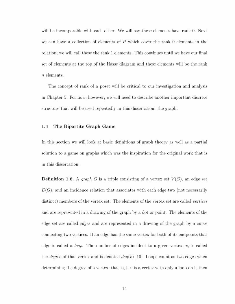
Definition 1.6. A graph G is a triple consisting of a vertex set V (G), an edge set
E(G), and an incidence relation that associates with each edge two (not necessarily
distinct) members of the vertex set. The elements of the vertex set are called vertices
and are represented in a drawing of the graph by a dot or point. The elements of the
edge set are called edges and are represented in a drawing of the graph by a curve
connecting two vertices. If an edge has the same vertex for both of its endpoints that
edge is called a loop. The number of edges incident to a given vertex, v, is called
the degree of that vertex and is denoted deg(v) [10]. Loops count as two edges when
determining the degree of a vertex; that is, if v is a vertex with only a loop on it then
14
deg(v) = 2.
We note that the definition allows for a graph to possibly be infinite, but we will
restrict our focus to finite graphs. Finite graphs have a finite number of vertices as
well as a finite number of edges. All of the graphs we consider will have no loops.
The Graph Game is a version of Take-Away played on a finite graph, G. When it
is her turn to move, a player may take either a single edge from the graph or otherwise
she may take a vertex and with it any edges that have that vertex as an endpoint.
The winner will be the player that removes the final piece of the graph. When we
remove pieces of the graph the new positions we reach are themselves graphs, and
these positions are referred to as subgraphs of G.
Definition 1.7. A subgraph of a graph G is a graph H such that V (H) is a subset
of V (G), E(H) is a subset of E(G), and the assignment of endpoint vertices to edges
in H is the same as in G [10].
There are a few types of graphs that will be particularly interesting in either the
discussion of the Graph Game here or in later chapters of the dissertation. One such
type is a path. A path is a sequence P = v0e1v1e2v2 . . . ekvk, k ≥ 2, whose terms are
alternating vertices and edges such that for 1 ≤ i ≤ k the endpoints of ei are vi−1
and vi and no vertices nor edges are repeated in the sequence. We say the path P
has length k. Another important graph for our purposes is the cycle. A cycle can
be defined as a closed path; that is, a cycle is a sequence C = v0e1v1e2v2 . . . ekv0,
k ≥ 2, whose terms are alternating vertices and edges such that for 1 ≤ i ≤ k− 1 the
endpoints of ei are vi−1 and vi, the endpoints of ek are v0 and vk−1, and no vertices
15

nor edges are repeated in the sequence (except for v0) [4]. While paths and cycles
can be graphs on their own, they can also be subgraphs of other graphs.
If every pair of vertices in G has a path between them then we say that G is
connected. Otherwise, we say G is disconnected. A graph G which is disconnected
is a collection of two or more connected graphs. We call these connected graphs the
components of G. We denote the number of components of G by ω(G). An edge, e,
is called a cut edge of G if ω(G− e) > ω(G); that is, a cut edge of G is an edge that
when removed from G increases the number of components of the resulting graph [4].
A connected graph that contains no cycles is called a tree. There are a few
standard facts about trees that will be helpful to know.
Theorem 1.8. If G is a tree with at least two vertices then G has at least two vertices
with degree 1.
Theorem 1.9. A connected graph G is a tree if and only if every edge is a cut edge.
In the Graph Game it is easy to see that a player could make a move on a connected
component of the graph for which the resulting position becomes disconnected. Since
the Graph Game is an impartial game, however, in these instances the single graph
game just becomes a sum of two or more graph games and a player may only make
a move in one component at a time.
The Graph Game has yet to be completely solved. Certain classes and types of
graphs have been investigated specifically, and of those we are particularly interested
in the results for bipartite graphs. A bipartite graph, G, is a graph such that V (G)
16

can be partitioned into two sets, V1(G) and V2(G), such that all edges in G must have
one endpoint in V1(G) and the other endpoint in V2(G).
The following theorem is due to R. Riehemann (2003) [7]; see also T. Khandhawit
and L. Ye (2011) [6].
Theorem 1.10 (Riehemann, 2003). Given a bipartite graph G, the nim-value of G
in the Graph Game depends on |V (G)| and |E(G)| as follows:
• If |V (G)| is even and |E(G)| is even, then g(G) = 0,
• If |V (G)| is odd and |E(G)| is even, then g(G) = 1,
• If |V (G)| is even and |E(G)| is odd, then g(G) = 2, and
• If |V (G)| is odd and |E(G)| is odd, then g(G) = 3.
This result was the primary inspiration for the games we investigate in Chapter
2 and Chapter 3. Riehemann proved through example that nim-values for graphs in
general can grow arbitrarily large, so Theorem 1.10 is quite exciting in that it says
a bipartite graph of any size has a nim-value determined exclusively by the parity of
its edges and vertices.
1.5 Polytopal Complexes
Another discrete structure that we will play a game of Take-Away on in this disserta-
tion is the polytopal complex. For definitions and theory about polytopal complexes,
see Lectures on Polytopes by Gunter M. Ziegler [11]. A polytopal complex is a finite,
nonempty collection C of convex polytopes in Rd such that
17

• If P ∈ C and Q is a (possibly empty) face of P , then Q ∈ C, and
• If P , Q ∈ C with P 6= Q, then P ∩Q is a common (possibly empty) face of P
and Q.
The dimension of a polytopal complex is the largest dimension of a polytope in C
[11]. Let fi denote the number of polytopes of dimension i in a polytopal complex K;
in situations where it might be unclear as to which complex we are referring, we will
use the notation fi(K). If K does not have any faces of dimension i then fi(K) = 0.
We will define C to be connected if its underlying graph is connected as in the
definition in Section 1.4. The vertices of the underlying graph are the f0 faces of C
and the edges are the f1 faces of C. As with graphs, if C is not connected we will
refer to its connected components.
We will prove some results about polytopal complexes in Chapter 4, but we will
focus on a specific class of polygonal complexes called polygonal complexes in Chapter
3 and sections of Chapter 2. A polygonal complex is a polytopal complex of dimension
2; that is, a polygonal complex is a polytopal complex which consists only of f0 faces
(vertices), f1 faces (edges), and f2 faces (polygons). Again, we will assume a polygonal
complex to be connected if its underlying graph is connected.
1.6 A Dissertation Road Map
We close Chapter 1 with a guide to what follows in this dissertation. In Chapter 2
we investigate Take-Away on hypergraphs and ultimately extend the Bipartite Graph
Game to hypergraphs with particular characteristics. We also consider examples of
18

hypergraphs that do not have the proper characteristics and investigate nim-values of
these examples. In Chapter 3 we turn our focus to a particular kind of hypergraph,
the polygonal complex. In particular, we look at playing Take-Away on a structure
that has an even-sided polygon with paths on vertices and edges extending from some
of the vertices of the polygon. These results stand in stark contrast to what we saw
in Chapter 2. In Chapter 4 we return to looking at graphs, but alter the rules of
Take-Away to allow a player to take more than one element of a graph at a time. We
then extend this altered version of Take-Away to polytopal complexes. Chapter 5
takes us to the world of posets, in which we look at results of Take-Away on a very
specific type of poset. In this chapter we also consider misere play on the poset, and
misere play on the sum of posets. Finally, in Chapter 6 we discuss some areas for
further investigation related to what we have discovered in Chapters 2 through 5.
The table that follows summarizes the main results of this dissertation.
19

Structure Game ResultsOddly Uniform Hypergraph Type 1 Take-Away Theorem 2.4Evenly Uniform Hypergraph Type 1 Take-Away Theorem 2.8
with a Marked ColoringEven Polygon with One Tail Type 2 Take-Away Theorem 3.5Even Polygon with Two Tails Type 2 Take-Away Theorem 3.6
(one of fixed length 1)Even Polygon with Two Tails Type 2 Take-Away Theorem 3.9
(one of fixed length 2)Even Polygon with Two Tails Type 2 Take-Away Theorem 3.10
(both of length ` ≥ 3)Quadrilateral with Four Tails Type 2 Take-Away Theorem 3.11
Even Polygon with a Tail Type 2 Take-Away Theorem 3.12at Every Vertex
Connected Graph Take-As-Much-As-You-Want Theorem 4.2with No Loops
Connected Polytopal Complex Take-As-Much-As-You-Want Theorem 4.4with d ≥ 3
Finite Rank-Complete Poset Take-Away Theorem 5.1Finite Rank-Complete Poset Misere Take-Away Theorem 5.2
Direct Sum of Finite Take-Away Theorem 5.3Rank-Complete Posets
20

Chapter 2 Hypergraph Games
In this chapter we will consider the game of Take-Away played on various hyper-
graphs. We will consider different classes of hypergraphs, look at specific examples
of these classes, and prove some results about their nim-values and overall strategy
for playing Take-Away for each class.
2.1 Game Description
A hypergraph, H = (V (H), E(H)), is a generalization of a graph in which each edge
(also referred to as hyperedge) e ∈ E(H) is incident to a nonempty finite subset of
V (H). Throughout this dissertation, we consider only hypergraphs with |V (H)| and
|E(H)| finite and each e ∈ E(H) is incident to at least two vertices. Similar to its
definition in a regular graph, we define the degree of a vertex in a hypergraph to be
the number of hyperedges incident to that vertex.
In this dissertation we will investigate two different versions of Take-Away on a
hypergraph. Recall that in Take-Away on a graph, a player has two options when it
is her turn to move: she can remove an edge, or she can remove a vertex and take
with it all edges which are incident to that vertex. The player who removes the last
vertex of the graph is the winner. On a hypergraph, the game is played in much the
same way. If a player chooses to take a vertex, all hyperedges containing that vertex
will also be removed. A player can also choose to take a hyperedge. An important
difference to note between Take-Away on a graph and Take-Away on a hypergraph
21

Figure 2.1: A hypergraph with hyperedges {A,B}, {A,C}, {B,C},{B,D}, {C,D},{A,B,C}, and {A,B,C,D}.
is that a hyperedge ei may be completely contained within another hyperedge ej. It
is this fact that will split the game into two types.
The first type of Take-Away on a hypergraph that we will discuss we will call
Type 1 Take-Away. In Type 1 Take-Away we will consider the hyperedges to be
independent objects. In this case, if a player chooses to remove ei, then ej (and
any other hyperedge that completely contains ei) will remain in the hypergraph to
be removed in another round of the game. As in the graph game, the player who
removes the last vertex from the hypergraph is declared the winner.
The second type of Take-Away on a hypergraph that we will discuss we will call
Type 2 Take-Away. In Type 2 Take-Away we will consider the hyperedges to be
linked by inclusion as subsets of the vertex set. In this case, if a player chooses to
remove ei, then ej (and any other hyperedge that completely contains ei) will also
be removed. As in the graph game, the player who removes the last vertex from the
hypergraph is declared the winner.
For example, consider the hypergraph pictured in Figure 2.1. This hypergraph
22

has vertex set V (H) = {A,B,C,D} and the following hyperedges: {A,B}, {A,C},
{B,C},{B,D}, {C,D}, {A,B,C}, and {A,B,C,D}. Suppose a player moves in the
game on this hypergraph by removing vertex A. In both Type 1 Take-Away and
Type 2 Take-Away, removing vertex A will also remove any hyperedge containing
vertex A, so the remaining hypergraph will have vertex set V (H)′ = {B,C,D} and
the hyperedges {B,C}, {B,D}, and {C,D}. Also, in either version of the game,
choosing to take the hyperedge with the largest cardinality, {A,B,C,D}, will not
remove any additional parts of the hypergraph.
If, instead, the player chose to remove the hyperedge {A,B}, then the two
different types of Take-Away would produce different subsequent positions of the
game. Under Type 1 play, the remaining graph would have vertex set V ′(H) =
V (H) = {A,B,C,D} and the hyperedges {A,C},{B,C}, {B,D}, {C,D}, and
{A,B,C,D}. Under Type 2 play, the remaining graph would have vertex set
V ′(H) = V (H) = {A,B,C,D} and the hyperedges {A,C},{B,C}, {B,D}, and
{C,D}, as {A,B,C,D} completely contains {A,B}.
In Chapter 2 we will focus on Type 1 Take-Away games. In Chapter 3 we will
focus on Type 2 Take-Away games.
2.2 Oddly Uniform Hypergraphs
A hypergraph is said to be oddly uniform if every hyperedge has odd cardinality
[2]. We can see that the hypergraph in Figure 2.1 is not oddly uniform because it
has hyperedges of even cardinality. The graph pictured in Figure 2.2, however, is
oddly uniform. The vertex set is V (H) = {E,F, J,K, L} and the hyperedges are
23

Figure 2.2: An oddly uniform hypergraph with hyperedges {E,F, J,K, L} and{E, J,K}.
{E,F, J,K, L} and {E, J,K}.
We now prove some useful lemmas about oddly uniform hypergraphs.
Lemma 2.1. Let H be an oddly uniform hypergraph. If |E(H)| is even and |V (H)|
is odd, then H must have at least one vertex with an even degree.
Proof. Assume, to the contrary, that every vertex in H has odd degree. Let ne be
the number of vertices incident to the hyperedge e. Since H is oddly uniform, ne is
odd for every e ∈ E(H). Now we have
∑v∈V (H)
deg(v) =∑
e∈E(H)
ne
Since each ne is odd and |E(H)| is even,∑
e∈E(H) ne is even. Hence∑
v∈V (H) deg(v)
is even. By the assumption, every vertex in H has odd degree, and |V (H)| is odd,
hence∑
v∈V (H) deg(v) is odd. Since we have a contradiction, we find that there must
be at least one vertex in H that has even degree.
24

Lemma 2.2. Let H be an oddly uniform hypergraph. If |E(H)| is odd and |V (H)| is
odd, then H must have at least one vertex with an odd degree.
Proof. Assume, to the contrary, that every vertex in H has even degree. Let ne be
the number of vertices incident to the hyperedge e. Since H is oddly uniform, ne is
odd for every e ∈ E(H). Now we have
∑v∈V (H)
deg(v) =∑
e∈E(H)
ne
Since each ne is odd and |E(H)| is odd,∑
e∈E(H) ne is odd. Hence∑
v∈V (H) deg(v)
is odd. By the assumption, every vertex in H has even degree, and |V (H)| is odd,
hence∑
v∈V (H) deg(v) is even. Since we have a contradiction, we find that there must
be at least one vertex in H that has odd degree.
Lemma 2.3. Let H be an oddly uniform hypergraph. If |E(H)| is odd and |V (H)| is
even, then H must have at least one vertex with an odd degree.
Proof. Assume, to the contrary, that every vertex in H has even degree. Let ne be
the number of vertices incident to the hyperedge e. Since H is oddly uniform, ne is
odd for every e ∈ E(H). Now we have
∑v∈V (H)
deg(v) =∑
e∈E(H)
ne
Since each ne is odd and |E(H)| is odd,∑
e∈E(H) ne is odd. Hence∑
v∈V (H) deg(v)
is odd. By the assumption, every vertex in H has even degree, and |V (H)| is even,
hence∑
v∈V (H) deg(v) is even. Since we have a contradiction, we find that there must
be at least one vertex in H that has odd degree.
25

With these lemmas in mind, we now turn our focus to Take-Away on oddly uniform
hypergraphs.
2.3 Take-Away on Oddly Uniform Hypergraphs
We will describe a complete solution to the game of Type 1 Take-Away on an oddly
uniform hypergraph. The strategy for playing can be determined by analyzing the
nim-values of the positions, and those nim-values can be determined based exclusively
on the number of vertices and the number of hyperedges in the hypergraph.
Theorem 2.4. Let H be an oddly uniform hypergraph. In the game of Type 1 Take-
Away on H, g(H) can be determined based on the number of vertices, V (H), and the
number of hyperedges, E(H). Specifically,
• if |V (H)| is even and |E(H)| is even, g(H) = 0
• if |V (H)| is odd and |E(H)| is even, g(H) = 1
• if |V (H)| is odd and |E(H)| is odd, g(H) = 2, and
• if |V (H)| is even and |E(H)| is odd, g(H) = 3.
Proof. The proof is by induction on v + e, where v = |V (H)| and e = |E(H)|.
Base case: Certainly it is clear that a hypergraph with no vertices (and thus no
hyperedges) is the winning position of the game, and hence has g(H) = 0.
Assume, then, that the theorem holds for v + e = i for all 0 ≤ i ≤ k and consider
a hypergraph, H, where v + e = k + 1. There are four cases to examine.
26

• Case 1: |V (H)| is even and |E(H)| is even. Consider the possible positions
that could be achieved after one move in the game. The resulting hypergraph,
H ′, could have one of the following combinations: |V (H ′)| is odd and |E(H ′)|
is even, |V (H ′)| is odd and |E(H ′)| is odd, or |V (H ′)| is even and |E(H ′)| is
odd. These positions have g(H ′) equaling 1, 3, and 2, respectively. Since these
are the only positions that can be reached from H after one move, g(H) = 0.
• Case 2: |V (H)| is odd and |E(H)| is even. The possible positions, H ′, resulting
after one move could have one of the following combinations: |V (H ′)| is even
and |E(H ′)| is even, |V (H ′)| is even and |E(H ′)| is odd, or |V (H ′)| is odd and
|E(H ′)| is odd. It is always possible to move to a H ′ with |V (H ′)| even and
|E(H ′)| even because H must have at least one vertex with an even degree (see
Lemma 2.1), and this H ′ has g(H ′) = 0. The remaining possibilities have g(H ′)
equaling 2 and 3, thus g(H) = 1.
• Case 3: |V (H)| is odd and |E(H)| is odd. The possible positions, H ′, resulting
after one move could have one of the following combinations: |V (H ′)| is even
and |E(H ′)| is even, |V (H ′)| is even and |E(H ′)| is odd, or |V (H ′)| is odd
and |E(H ′)| is even. Since H has an odd number of hyperedges it is certainly
possible to remove one hyperedge and result in a H ′ with |V (H ′)| odd and
|E(H ′)| even; this H ′ has g(H ′) = 1. It is always possible to move to a H ′ with
|V (H ′)| even and |E(H ′)| even because H must have at least one vertex with
an odd degree (see Lemma 2.2), and this H ′ has g(H ′) = 0. The only other
position that is possible has g(H ′) = 3. Therefore g(H) = 2.
27

• Case 4: |V (H)| is even and |E(H)| is odd. The possible positions, H ′, resulting
after one move could have one of the following combinations: |V (H ′)| is even
and |E(H ′)| is even, |V (H ′)| is odd and |E(H ′)| is odd, or |V (H ′)| is odd and
|E(H ′)| is even. Since H has an odd number of hyperedges, it is certainly
possible to remove one hyperedge and result in a H ′ with |V (H ′)| even and
|E(H ′)| even; this H ′ has g(H ′) = 0. It is always possible to move to a position
H ′ with |V (H ′)| odd and |E(H ′)| even because H must have a vertex with odd
degree (see Lemma 2.3), and this H ′ has g(H ′) = 1. It is also always possible to
move to a position H ′ with |V (H ′)| is odd and |E(H ′)| is odd because H must
have a vertex of even degree (see Lemma 2.3, again), and for this H ′ g(H ′) = 2.
Therefore g(H) = 3.
This result is exciting because there are special cases of oddly uniform hypergraphs
that come up somewhat naturally and would be reasonable choices for structures on
which to play a game of Take-Away. We describe some in the next section.
2.4 Corollaries and Related Games
In this section, we will consider some of the special cases of oddly uniform hyper-
graphs.
28
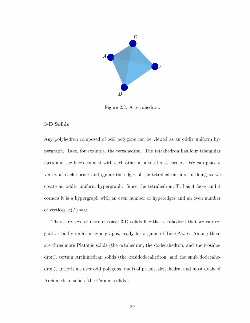
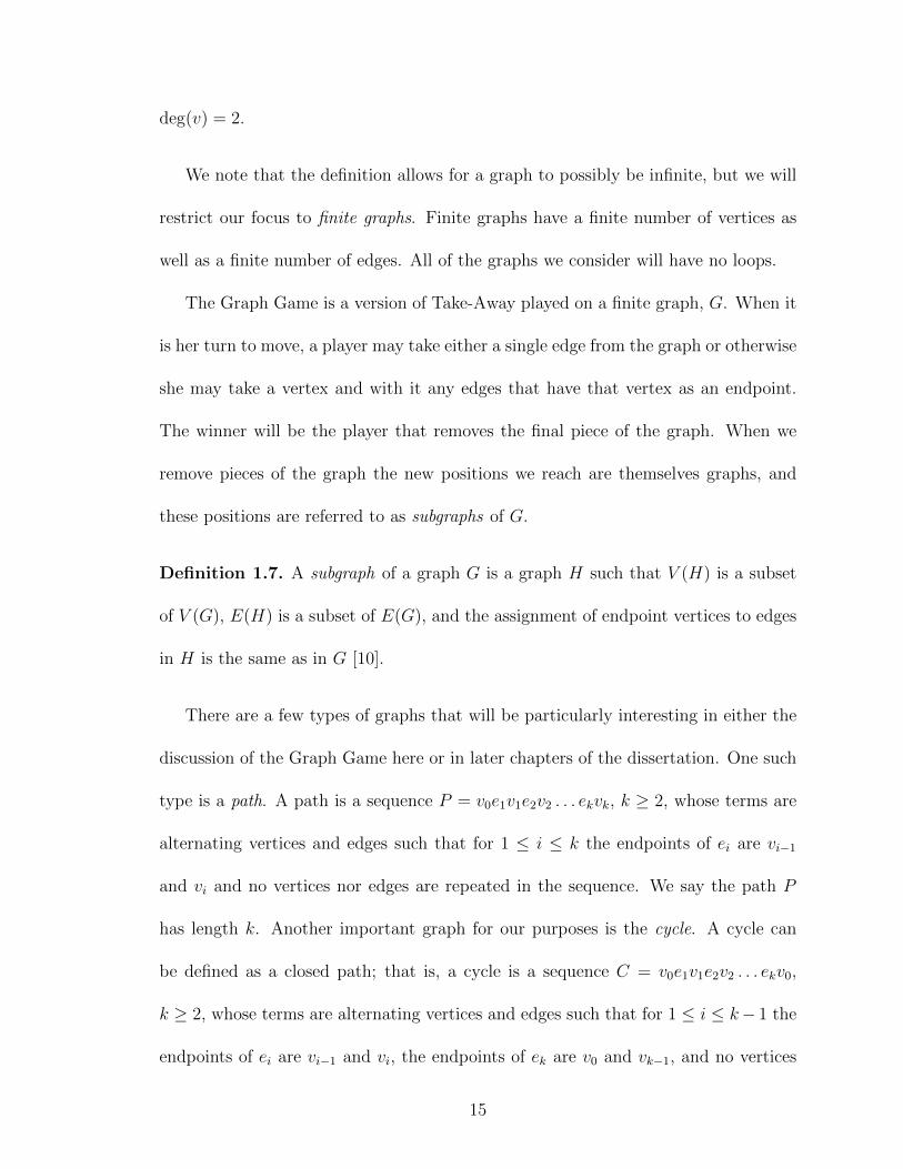
Figure 2.3: A tetrahedron.
3-D Solids
Any polyhedron composed of odd polygons can be viewed as an oddly uniform hy-
pergraph. Take, for example, the tetrahedron. The tetrahedron has four triangular
faces and the faces connect with each other at a total of 4 corners. We can place a
vertex at each corner and ignore the edges of the tetrahedron, and in doing so we
create an oddly uniform hypergraph. Since the tetrahedron, T , has 4 faces and 4
corners it is a hypergraph with an even number of hyperedges and an even number
of vertices, g(T ) = 0.
There are several more classical 3-D solids like the tetrahedron that we can re-
gard as oddly uniform hypergraphs, ready for a game of Take-Away. Among them
are three more Platonic solids (the octahedron, the dodecahedron, and the icosahe-
dron), certain Archimedean solids (the icosidodecahedron, and the snub dodecahe-
dron), antiprisims over odd polygons, duals of prisms, deltahedra, and most duals of
Archimedean solids (the Catalan solids).
29
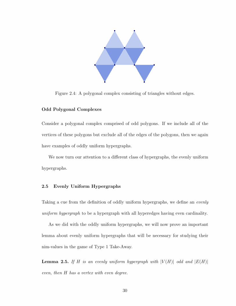
Figure 2.4: A polygonal complex consisting of triangles without edges.
Odd Polygonal Complexes
Consider a polygonal complex comprised of odd polygons. If we include all of the
vertices of these polygons but exclude all of the edges of the polygons, then we again
have examples of oddly uniform hypergraphs.
We now turn our attention to a different class of hypergraphs, the evenly uniform
hypergraphs.
2.5 Evenly Uniform Hypergraphs
Taking a cue from the definition of oddly uniform hypergraphs, we define an evenly
uniform hypergraph to be a hypergraph with all hyperedges having even cardinality.
As we did with the oddly uniform hypergraphs, we will now prove an important
lemma about evenly uniform hypergraphs that will be necessary for studying their
nim-values in the game of Type 1 Take-Away.
Lemma 2.5. If H is an evenly uniform hypergraph with |V (H)| odd and |E(H)|
even, then H has a vertex with even degree.
30

Proof. To the contrary, assume that every vertex in H has odd degree. Let ne be the
number of vertices incident to the hyperedge e. Since H is evenly uniform, ne is even
for every e ∈ E(H). Now we have
∑v∈V (H)
deg(v) =∑
e∈E(H)
ne.
Since each ne is even and |E(H)| even,∑
e∈E(H) ne is even. Hence∑
v∈V (H) deg(v)
is even. By the assumption, every vertex in H has odd degree, and |V (H)| is odd,
hence∑
v∈V (H) deg(v) is odd. Since we have a contradiction, we find that there must
be at least one vertex in H that has even degree.
Some additional lemmas will be useful for our proof to describe nim-values of
evenly uniform hypergraphs in the game of Type 1 Take-Away, but in order for these
to hold we will need to introduce a new coloring condition on the hypergraphs.
2.6 Hypergraph Colorings
The classic definition of a hypergraph coloring is a coloring of the vertices such that
no hyperedge has a monochromatic coloring. Of course, this is consistent with the
standard coloring of a graph [10]. For a hypergraph where the hyperedges have 3
or more vertices, this definition means that every hyperedge must have at least two
colors, but the same color can be repeated on multiple vertices within the same
hyperedge. We note that this definition is for hypergraphs in general, not just evenly
uniform hypergraphs.
We will call a hypergraph coloring a marked coloring if there is an odd number
of vertices on each hyperedge which receive a particular color—call this color c1. Let
31

Figure 2.5: An evenly uniform hypergraph with a standard coloring.
H be a hypergraph and C1 ⊆ V (H) be the subset of vertices receiving color c1. It
is important to notice that if we sum the degrees of the vertices in C1, since each
hyperedge of H has an odd number of marked vertices, we have that
∑v∈C1
deg(v) ≡ |E(H)| (mod 2).
Again, it is important to note that a marked coloring is not exclusive to an evenly
uniform hypergraph. There are evenly uniform hypergraphs that do not have marked
colorings as well as hypergraphs which exhibit a marked coloring that are not evenly
uniform.
In Figure 2.6 we see an example of an evenly uniform hypergraph which has a
marked coloring. The vertices in red are the subset C1, and the other vertices are
marked in black. This particular marked coloring allows each hyperedge to have
exactly one red vertex, so∑
v∈C1deg(v) = |E(H)| here.
32

Figure 2.6: An evenly uniform hypergraph with a marked coloring.
Figure 2.7: Another evenly uniform hypergraph with a marked coloring.
33

Figure 2.8: A hypergraph that does not have a marked coloring.
In Figure 2.7 we have an example of an evenly uniform hypergraph which has
a marked coloring, but it cannot be colored in such a way that each hyperedge has
only one vertex with color c1. In this hypergraph we have the hyperedges {A,B},
{A,C}, {B,C}, {B,D}, {C,D}, {A,C,E, F}, and {B,D,G,H}. Suppose we could
color this hypergraph so that every hyperedge has only one vertex with color c1. The
problem lies within the chain of hyperedges {A,B}, {B,C}, and {C,D}. In order to
properly color this chain we must give A and C the same color and B and D the same
color. Unfortunately, however, A and C are both on hyperedge {A,C,E, F} and B
and D are both on hyperedge {B,D,G,H}. Properly coloring the hyperedge path
{A,B}, {B,C}, {C,D} prevents our ability to only allow one vertex with color c1
on every hyperedge; however, we can give each hyperedge an odd number of vertices
colored with c1 as shown.
In Figure 2.8 we have an example of an evenly uniform hypergraph that cannot be
colored with a marked coloring. To the contrary, suppose that it could. Without loss
34

of generality, we could choose any vertex to be the first to receive color c1, so we will
choose vertex D. So the hyperedges {A,C,D,E} and {B,C,D, F} have one vertex
with color c1. Now hyperedge {A,B,E, F} needs to have either one or three vertices
colored with color c1. If we color only one vertex, say vertex A, then hyperedge
{A,C,D,E} will have two vertices with color c1. Since a marked coloring has an
odd number of vertices on each edge receiving the special color, we must choose a
third vertex on hyperedge {A,C,D,E} to color with c1. Choosing either vertex C
or vertex E will result in one of the other hyperedges to now have two vertices with
color c1. As we continue to add vertices to the set C1 we will always force at least
one of the hyperedges to have an even number of vertices with color c1, hence this
hypergraph does not have a marked coloring.
Given this definition of marked coloring, we can now prove our other necessary
lemmas.
Lemma 2.6. If H is an evenly uniform hypergraph with a marked coloring, |V (H)|
is even, and |E(H)| is odd, then H has a vertex of odd degree.
Proof. Assume, to the contrary, that every vertex in H has even degree. Since
∑v∈C1
deg(v) ≡ |E(H)| (mod 2),
E(H) must be even. But |E(H)| is odd. Since we have a contradiction, it must be
that there is at least one vertex in H that has odd degree.
Lemma 2.7. If H is an evenly uniform hypergraph with a marked coloring, |V (H)| ≥
3 and is odd, and |E(H)| is odd, then H has at least one even degree vertex and at
35

least one odd degree vertex.
Proof. Let ne be the number of vertices in the hyperedge e. Since H is evenly uniform,
ne is even for every e ∈ E(H). Now we have
∑v∈V (H)
deg(v) =∑
e∈E(H)
ne.
Since each ne is even,∑
e∈E(H) ne is even. Hence∑
v∈V (H) deg(v) is even. Since there
is an odd number of vertices, this implies that there is at least one vertex with even
degree in V (H).
Since∑
v∈C1deg(v) ≡ |E(H)| (mod 2), and E(H) is odd,
∑v∈C1
deg(v) must
also be odd. Therefore there must be at least one odd degree vertex in C1.
As the earlier lemmas were useful in analyzing the game of Type 1 Take-Away on
oddly uniform hypergraphs, the lemmas in this section will be used to help prove a
strategy for game play of Type 1 Take-Away on evenly uniform hypergraphs.
2.7 Take-Away on Evenly Uniform Hypergraphs
Recall that for an oddly uniform hypergraph that the game of Type 1 Take-Away is
completely solved. Unfortunately, we cannot say the same thing for evenly uniform
hypergraphs. In fact, if Take-Away on evenly uniform hypergraphs were completely
solved then the solution to the graph game would follow as a corollary as every graph
could be viewed as a 2-uniform hypergraph.
Since there are certain cases where the game of Take-Away on a graph is solved,
it is logical to try to extend those ideas to the game of Take-Away on an evenly
36

uniform hypergraph. Recall that Take-Away is completely solved on bipartite graphs
(see Theorem 1.10), so a reasonable next step is to find an appropriate condition to
impose on the hypergraphs that mimics the quality that bipartite graphs have that
allows the game to be solvable.
As it turns out, that condition is that the hypergraph have a marked coloring.
This should not be surprising, as a marked coloring is one possibility of an extension
of a bipartite coloring to a hypergraph. In fact, if we again consider a graph as
a 2-uniform hypergraph then the ones that have marked colorings are exactly the
bipartite graphs.
Theorem 2.8. Let H be an evenly uniform hypergraph with a marked coloring. In
the game of Type 1 Take-Away on H, g(H) can be determined based on the number
of vertices, |V (H)|, and the number of hyperedges, |E(H)|. Specifically,
• if |V (H)| is even and |E(H)| is even, g(H) = 0
• if |V (H)| is odd and |E(H)| is even, g(H) = 1
• if |V (H)| is even and |E(H)| is odd, g(H) = 2, and
• if |V (H)| is odd and |E(H)| is odd, g(H) = 3.
Proof. The proof is by induction on v + e, where v = |V (H)| and e = |E(H)|.
Base case: Certainly it is clear that a hypergraph H with no vertices (and hence
no hyperedges) is the winning position of the game, and hence g(H) = 0.
37

Assume, then, that the theorem holds for evenly uniform hypergraphs with marked
colorings where v + e = i, 0 ≤ i ≤ k. Consider an evenly uniform hypergraph, H,
which has a marked coloring and where v+e = k+1. There are four cases to examine.
• Case 1: |V (H)| is even and |E(H)| is even. Consider the possible positions that
could be achieved after one move in the game. The resulting hypergraph, H ′,
could have one of the following combinations: |V (H ′)| is even and |E(H ′)| is
odd, |V (H ′)| is odd and |E(H ′)| is odd, or |V (H ′)| is odd and |E(H ′)| is even.
These positions have g(H ′) equal to 2, 3, and 1, respectively. Since these are
the only positions that could be reached from H after one move, g(H) = 0.
• Case 2: |V (H)| is odd and |E(H)| is even. The possible positions, H ′, resulting
after one move could have one of the following combinations: |V (H ′)| is even
and |E(H ′)| is even, |V (H ′)| is odd and |E(H ′)| is odd, or |V (H ′)| is even and
|E(H ′)| is odd. In the first instance, since H is guaranteed to have a vertex of
even degree (see Lemma 2.5) it is certainly possible to remove this vertex and
result in a H ′ with |V (H ′)| even and |E(H ′)| even; this H ′ has g(H ′) = 0. The
other two possibilities, if achievable, have g(H ′) equal to 3 and 2, respectively.
Therefore g(H) = 1.
• Case 3: |V (H)| is even and |E(H)| is odd. The possible positions, H ′, resulting
after one move could have one of the following combinations: |V (H ′)| is even
and |E(H ′)| is even, |V (H ′)| is odd and |E(H ′)| is even, or |V (H ′)| is odd and
|E(H ′)| is odd. It is always possible to move to a H ′ with |V (H ′)| even and
|E(H ′)| even because you can remove a single hyperedge; this H ′ has g(H ′) = 0.
38

It is also always possible to move to a H ′ with |V (H ′)| odd and |E(H ′)| even
because H must have a vertex with odd degree (see Lemma 2.6), and this H ′
has g(H ′) = 1. The third combination—|V (H ′)| odd and |E(H ′)| odd—is only
possible when H has an even degree vertex. If this particular H ′ is possible, it
has g(H ′) = 3. Therefore g(H) = 2.
• Case 4: |V (H)| is odd and |E(H)| is odd. The possible positions, H ′, resulting
after one move could have one of the following combinations: |V (H ′)| is even
and |E(H ′)| is even, |V (H ′)| is odd and |E(H ′)| is even, or |V (H ′)| is even and
|E(H ′)| is odd. Since H has an odd number of hyperedges it is certainly possible
to remove one hyperedge and result in a H ′ with |V (H ′)| odd and |E(H ′)| even;
this H ′ has g(H ′) = 1. It is always possible to move to a H ′ with |V (H ′)| even
and |E(H ′)| odd because H must have at least one vertex with an even degree
(see Lemma 2.7), and this H ′ has g(H ′) = 2. It is also always possible to move
to a H ′ with |V (H ′)| even and |E(H ′)| even because every H must have a vertex
with odd degree (see Lemma 2.7, again), and this H ′ has g(H ′) = 0. Therefore
g(H) = 3.
Figure 2.8 has been shown to not have a marked coloring therefore we cannot use
the results of Theorem 2.8 in order to find its nim-value and determine whether or
not it is a winning position in a game of Type 1 Take-Away. Does the nim-value for
Figure 2.8 agree with what this theorem predicts despite not being able to use it?
If so, that might imply that there is a stronger condition that could be found which
39

would include both the hypergraphs which are marked colorable and structures like
Figure 2.8.
It turns out that the nim-value for Figure 2.8 does not agree with the predicted
value by these theorems. Since the hypergraph has an even number of vertices and
an odd number of hyperedges, the theorem would predict it to have nim-value 2. The
hypergraph is small, and we can analyze subsequent moves quickly and easily. Based
on the symmetry in the hypergraph, we can see that there are only two unique moves
that could be made in the game of Type 1 Take-Away: a player could remove a vertex,
taking with it two hyperedges, or the player could remove one of the hyperedges and
leave all vertices as well as the two remaining hyperedges. In the first case, the
structure that is left behind will be a single hyperedge on 4 vertices and an isolated
vertex. This position can be given a marked coloring, so by Theorem 2.8, this position
has nim-value 3. In the second case, the structure that is left behind will be 6 vertices
with two non-overlapping hyperedges, each on 4 vertices. Again, this hypergraph can
be given a marked coloring, so by Theorem 2.8, this position has nim-value 0. So,
according to Definition 1.2 we conclude that the nim-value for Figure 2.8 is 1. Thus
if structures like this hypergraph have a pattern to their nim-values it is not the
same pattern as the one we have shown for evenly uniform hypergraphs with marked
colorings.
Marked evenly uniform hypergraphs can be created from any polygonal complex.
It is important to note, however, that these evenly uniform hypergraphs are not
equivalent to the polygonal complexes from which they are made. The construction
is as follows: Place a new vertex in the center of every polygon, then extend a line
40
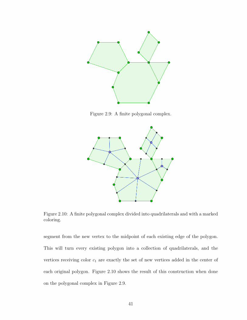
Figure 2.9: A finite polygonal complex.
Figure 2.10: A finite polygonal complex divided into quadrilaterals and with a markedcoloring.
segment from the new vertex to the midpoint of each existing edge of the polygon.
This will turn every existing polygon into a collection of quadrilaterals, and the
vertices receiving color c1 are exactly the set of new vertices added in the center of
each original polygon. Figure 2.10 shows the result of this construction when done
on the polygonal complex in Figure 2.9.
41
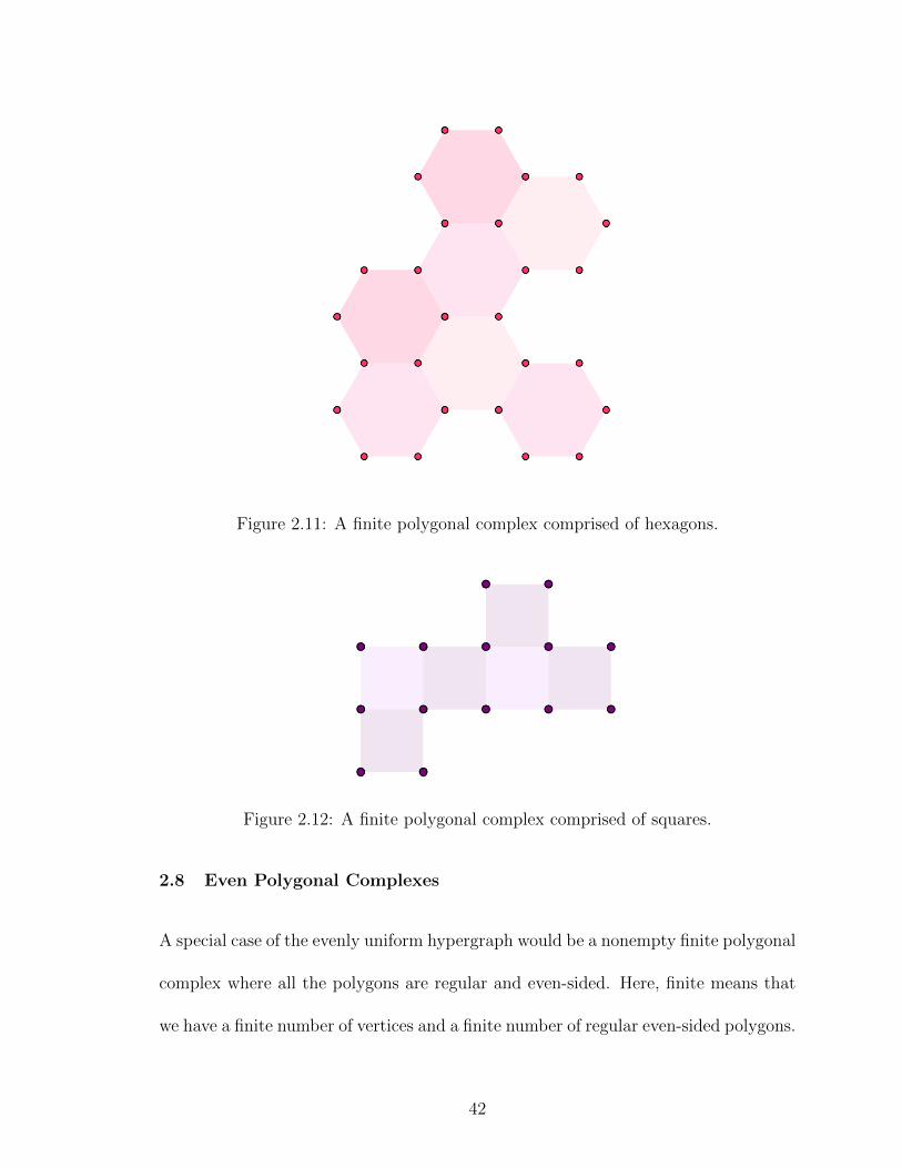
Figure 2.11: A finite polygonal complex comprised of hexagons.
Figure 2.12: A finite polygonal complex comprised of squares.
2.8 Even Polygonal Complexes
A special case of the evenly uniform hypergraph would be a nonempty finite polygonal
complex where all the polygons are regular and even-sided. Here, finite means that
we have a finite number of vertices and a finite number of regular even-sided polygons.
42
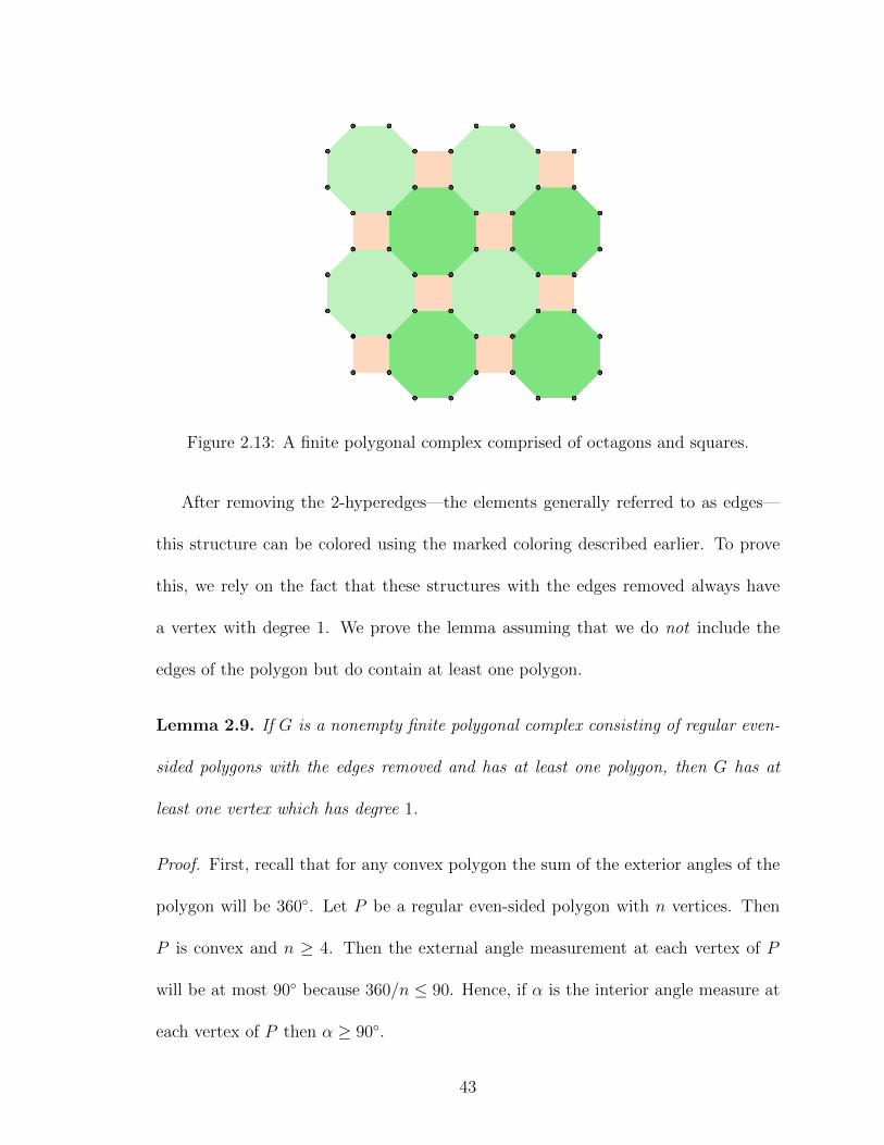
Figure 2.13: A finite polygonal complex comprised of octagons and squares.
After removing the 2-hyperedges—the elements generally referred to as edges—
this structure can be colored using the marked coloring described earlier. To prove
this, we rely on the fact that these structures with the edges removed always have
a vertex with degree 1. We prove the lemma assuming that we do not include the
edges of the polygon but do contain at least one polygon.
Lemma 2.9. If G is a nonempty finite polygonal complex consisting of regular even-
sided polygons with the edges removed and has at least one polygon, then G has at
least one vertex which has degree 1.
Proof. First, recall that for any convex polygon the sum of the exterior angles of the
polygon will be 360◦. Let P be a regular even-sided polygon with n vertices. Then
P is convex and n ≥ 4. Then the external angle measurement at each vertex of P
will be at most 90◦ because 360/n ≤ 90. Hence, if α is the interior angle measure at
each vertex of P then α ≥ 90◦.
43

Now, let G be a nonempty finite polygonal complex consisting of regular even-
sided polygons with the edges removed and at least one polygon. Delete all vertices
of G that are not incident to any polygon to form G′, and let H be the convex hull of
G′. Let x ∈ V (G′) such that x is a corner of H. Since x is a corner of H, the interior
angles of all polygons in G′ which meet at x must sum to be less than 180◦. Then,
since the measure of the interior angles of all polygons in G′ must be greater than or
equal to 90◦, it is not possible for more than one polygon to be incident to vertex x.
Therefore we can conclude that vertex x has degree 1 in G′, and hence x has degree
1 also in G.
The regularity of the polygons is critical in the argument for Lemma 2.9. Clearly,
if we do not have regularity then we cannot make the claims about the measures of
the interior angles being at least 90◦. We can refer to Figure 2.8 to see an example of
a nonempty finite polygonal complex which does not use regular polygons and does
not have a vertex of degree 1.
Lemma 2.9 guarantees an odd degree vertex in any a nonempty finite polygonal
complex consisting of regular even-sided polygons with the edges removed and at
least one polygon. This was exactly the condition we needed the marked coloring
for before, so now we can use this lemma to prove that a finite polygonal complex
consisting of regular even-sided polygons with the edges removed will have a marked
coloring.
Theorem 2.10. If all edges are removed from a finite polygonal complex consisting
of regular even-sided polygons and at least one polygon then the resulting G has a
44

marked coloring.
Proof. Let G be as described. The proof is by induction on |V (G)|.
Base Case: The smallest G that meets the requirements is a square on four ver-
tices. Certainly this complex can receive a marked coloring by choosing one of the
four vertices to receive color c1.
Assume that for all G with |V (G)| = i, 4 ≤ i ≤ k, that G has a marked coloring.
Consider a finite polygonal complex consisting of regular even-sided polygons and at
least one polygon and remove all of the edges to form H with |V (H)| = k + 1. We
are guaranteed by Lemma 2.9 that H has a vertex, say v, with degree 1. Removing
v and its incident polygon leaves H ′ with |V (H ′)| = k, so by induction H ′ has a
marked coloring. Now, replace v and its incident polygon. If the polygon is properly
marked under the coloring on H ′, we are done. If the polygon has an even number
of vertices colored with c1 under the coloring on H ′ then color v with c1 so that the
polygon now has an odd number of marked vertices.
A direct corollary of Theorem 2.10 is a result that is a slight variant of Theorem
2.8.
Corollary 2.11. For a game of Type 1 Take-Away played on a finite nonempty
polygonal complex comprised of regular even-sided polygons with the edges removed,
F , g(F ) can be determined based on the number of vertices of F, |V (F )|, and the
number of polygons, |P (F )|. Specifically,
• if |P (F )| is even and |V (F )| is even, then g(F ) = 0
45

• if |P (F )| is even and |V (F )| is odd, then g(F ) = 1
• if |P (F )| is odd and |V (F )| is even, then g(F ) = 2, and
• if |P (F )| is odd and |V (F )| is odd, then g(F ) = 3.
Proof. Let F be a finite nonempty polygonal complex comprised of regular even-sided
polygons with the edges removed. By Theorem 2.10, F has a marked coloring. Thus
we can apply Theorem 2.8.
2.9 Hypergraphs With Both Odd And Even Hyperedges
Thus far this chapter has focused on separating hypergraphs into those whose hy-
peredges all have an odd number of vertices, and those whose hyperedges all have
an even number of vertices and a marked coloring. What conclusions, if any, can
be drawn for hypergraphs which contain both even and odd hyperedges? We will
consider this question in this section.
To attempt to answer the question, we look at a complete analysis of Type 1 Take-
Away on the truncated tetrahedron with the edges removed. Figures 2.14 through
2.19 show Schlegel diagrams for all the combinatorial types of connected positions
with at least one hyperedge we can obtain in a game of Type 1 Take-Away on the
truncated tetrahedron. A Schlegel diagram is a projection of, in this case, a poly-
hedron into the plane through one of its faces [11]. Having this two dimensional
representation of the three dimensional figure makes it easier to carry out the hyper-
edge and vertex removal analysis. In the figures, if the front hexagon—the hyperedge
46

Figure 2.14: Schlegel diagrams of positions obtained from the truncated tetrahedronthat have nim-value 0.
we imagine looking through to create the Schlegel diagram—is present we see a pink
shading.
We also note that the truncated tetrahedron has a marked coloring. Choose one
of the triangles and give all three vertices of that triangle color c1. Then, on the
hexagon opposite that triangle, choose every other vertex to receive color c1. This
coloring, seen in Figure 2.20, puts an odd number of vertices with color c1—shown in
red—on each polygon, not just the even polygons.
Recall that for the oddly uniform hypergraphs and the evenly uniform hypergraphs
with a marked coloring that the nim-value for any given position can be determined
based on the cardinality of the vertex set and the cardinality of the edge set. The same
cannot be said for the truncated tetrahedron, and therefore cannot be said in general
47
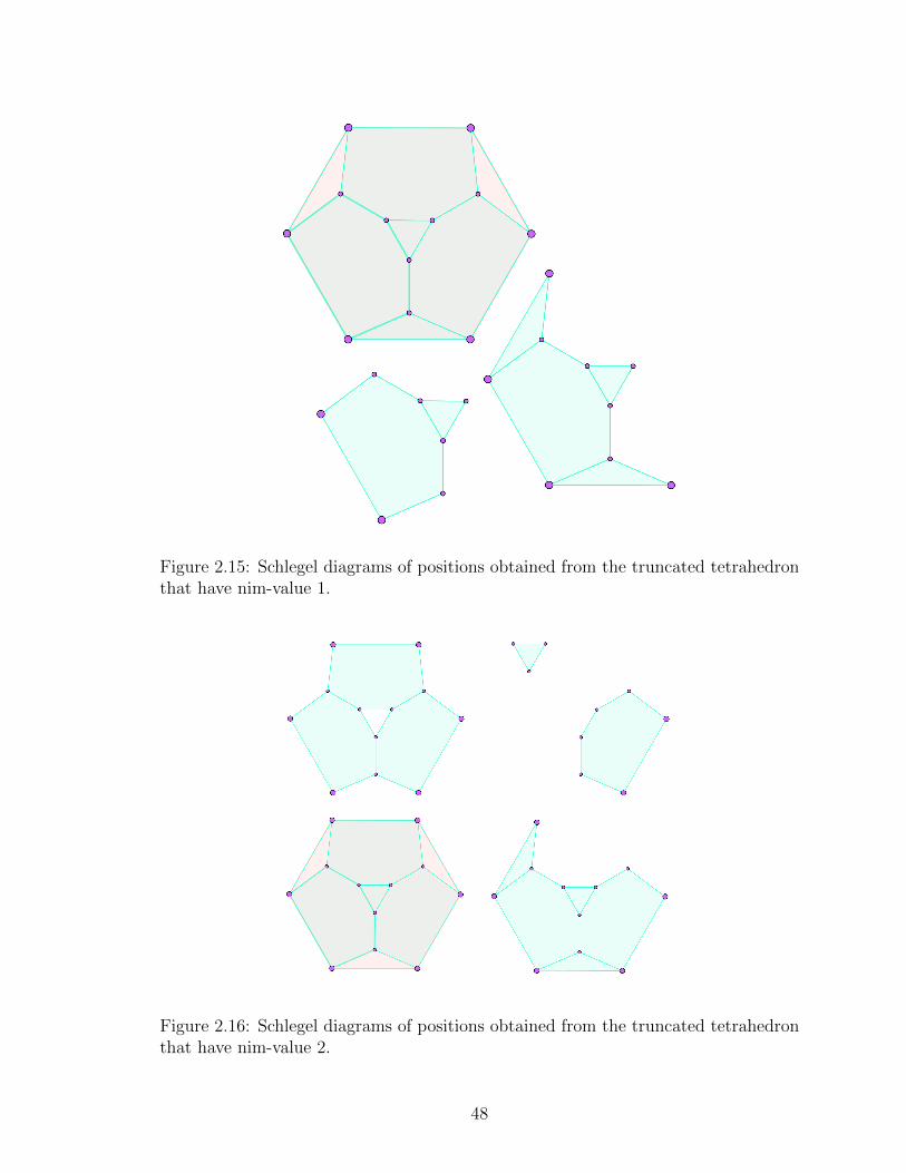
Figure 2.15: Schlegel diagrams of positions obtained from the truncated tetrahedronthat have nim-value 1.
Figure 2.16: Schlegel diagrams of positions obtained from the truncated tetrahedronthat have nim-value 2.
48

Figure 2.17: Schlegel diagrams of positions obtained from the truncated tetrahedronthat have nim-value 3.
Figure 2.18: Schlegel diagrams of positions obtained from the truncated tetrahedronthat have nim-value 4.
49

Figure 2.19: Schlegel diagrams of positions obtained from the truncated tetrahedronthat have nim-value 6.
Figure 2.20: Schlegel diagram of a truncated tetrahedron showing a marked coloring.
50

Figure 2.21: A table with observed data about truncated tetrahedron game positionswith different nim-values.
for hypergraphs with both odd cardinality and even cardinality hyperedges, even if
they can be marked. This can immediately be seen given that we now have positions
with nim-value 4 and positions with nim-value 6. Considering that these positions
could be paired with an isolated vertex, we then have positions which, through nim-
sum, have nim-value 5 and nim-value 7. We now have eight unique nim-values; could
nim-values, then, be controlled by the cardinality of three specific parameters of the
hypergraph?
From the parameters we observed, this does not seem to be the case. In Figure
2.21 we see for each of the positions pictured in the truncated tetrahedron figures
above, we have examined fourteen parameters:
• the number of hexagons,
• the number of triangles,
51

• the total number of polygons,
• the total number of vertices,
• the total number of odd degree vertices,
• the total number of even degree vertices,
• the number of vertices incident to an odd number of hexagons,
• the number of vertices incident to an even number of hexagons,
• the number of vertices incident to an odd number of triangles,
• the number of vertices incident to an even number of triangles,
• the number of vertices incident to both an even number of hexagons and trian-
gles,
• the number of vertices incident to an even number of hexagons and an odd
number of triangles,
• the number of vertices incident to an odd number of hexagons and an even
number of triangles, and
• the number of vertices incident to both an odd number of hexagons and an odd
number of triangles.
The values with even cardinality are shaded green and the values with odd cardi-
nality are shaded orange. Looking at the table we can see examples of positions that
match parity on all fourteen parameters yet have different nim-values. For example,
52

Figure 2.22: A hexagon with its edges.
the lowest position on the table with nim-value 4 and the lowest position on the table
with nim-value 6 have the same parities across the table.
2.10 Type 1 Take-Away versus Type 2 Take-Away
We end this chapter by considering the results about oddly uniform hypergraphs and
evenly uniform hypergraphs and how they do not hold under the rules of Type 2
Take-Away. Recall that in Type 2 Take-Away that if a hyperedge, e, is removed then
any other hyperedge containing e will also be removed.
For example, consider the hypergraph, H, in Figure 2.22. This
hypergraph has vertex set {A,B,C,D,E, F} and hyperedge set
{{A,B}, {B,C}, {C,D}, {D,E}, {E,F}, {A,F}, {A,B,C,D,E, F}}. This hy-
pergraph is also markable; vertices A, C, and E can be given color c1 and then every
53
hyperedge has an odd number of marked vertices. By Theorem 2.8 we know that
g(H) = 2 under the rules of Type 1 Take-Away.
Consider H under the rules of Type 2 Take-Away. Due to the symmetry of
H there are only three unique positions a player could move to via one move in
the game. She could remove the hyperedge {A,B,C,D,E, F}—the hexagon—which
leaves a position H ′ that is a bipartite graph with six vertices and six edges; hence,
g(H ′) = 0. She could remove an edge, taking with it the hexagon, which leaves a
position H ′ that is a bipartite graph with six vertices and five edges; hence, g(H ′) = 2.
Lastly, she could remove a vertex, taking with it two edges and the hexagon, which
leaves a position H ′ that is a bipartite graph with five vertices and four edges; hence,
g(H ′) = 1. So, by Definition 1.2, we find g(H) = 3 under the rules of Type 2
Take-Away.
A critical observation that is made in the proofs of Theorem 2.4 and Theorem 2.8
is that making a move in an oddly uniform hypergraph or a marked evenly uniform
hypergraph changes the parity of at least one of |V (G)| or |E(G)|. In particular, if
G is a hypergraph with |V (G)| even and |E(G)| odd then there is no single move
that could be made in the game of Take-Away Type 1 that will yield a position G′
which also has |V (G)| even and |E(G)| odd. Were this the case, then we could not
determine the nim-value of a position based on these parities alone. In the hexagon
in Figure 2.22 under Take-Away Type 2, however, we can remove an edge and move
to a position with |V (G)| even and |E(G)| odd since removing the edge also removes
the hexagon. Therefore the proofs used for the Type 1 Take-Away games do not
carry over to the Type 2 Take-Away games.
54

In the next chapter we will look at some results of games played with Type 2
Take-Away.
Copyright c© Kristen M. Barnard, 2017.
55
Chapter 3 Polygon Games
In the previous chapter we saw results about the game of Type 1 Take-Away when
played on very particular types of hypergraphs as well as Type 1 Take-Away on polyg-
onal complexes with the edges removed. In this chapter we will continue to investigate
the game of Take-Away played on polygonal complexes; this time, though, we will be
using the rules of Type 2 Take-Away. These games have yet to be completely solved,
but we do have some interesting partial results to share.
First we will discuss the basics of game play on the polygonal complexes. From
there we will start with small cases and build up, proving sometimes surprising results
about the cases as we go along. We also will look at a very interesting yet currently
unsolved case.
3.1 Game Play
As the reader can surely presume, the evenly uniform hypergraphs and oddly uniform
hypergraphs were not where we began our investigation. In fact, the first question
we investigated was about playing Take-Away on a portion of a square grid such as
the one pictured in Figure 3.1. The goal at that time was to solve the game played
on a grid of squares, then move on to other finite portions of a tiling of the plane.
These structures are special types of polygonal complexes. The difference between
these structures and the polygonal complexes we considered in the previous chapter
is that the polygons we are considering here also include the 2-vertex hyperedges,
56

Figure 3.1: A portion of a square grid.
Figure 3.2: A portion of a square grid with even degree corner vertices.
57
the components we usually call edges. These complexes will not always meet the
requirements of the theorems of the previous chapter, and even if they do we saw
that the nim-values under Type 2 Take-Away can differ from the nim-values under
Type 1 Take-Away.
Recall that the game of Take-Away on a graph is still unsolved, and it is known
that the nim-values of a general graph could grow without bound [7, 6]. Take-Away on
a bipartite graph, however, is completely solved with well-behaved nim-values as we
saw in Theorem 1.10. Because of this, when investigating Take-Away on a polygonal
complex, it is logical to start with a polygonal complex where if the polygonal faces
were removed—leaving the edges and vertices—the underlying graph is bipartite. Of
course, to try to understand the game at large, it is necessary to study small cases.
For this game of Type 2 Take-Away on a polygonal complex, we begin with an
even polygon. Game play is is similar to play in the regular graph game. When it
is her turn to play, a player can remove the polygonal face, an edge—taking with it
all polygonal faces incident to that edge, or a vertex—taking with it all edges and
polygonal faces incident to the vertex. We note here that in this chapter when we
refer to an edge we are talking about a curve which connects exactly two vertices,
which is the standard definition for edges in graphs. Further, when we reference
E(K) in a polygonal complex K, we are referring to the set of ordinary edges on two
vertices, and this set does not include the polygons of the complex.
We are almost ready to discuss the results about Type 2 Take-Away on an even
polygon with tails. However, before we can prove anything about an even polygon
with a single tail, we must know the nim-value of the polygon without a tail. This
58

result is in Theorem 3.1.
Theorem 3.1. Let P be an even polygon with n vertices. Then, in Type 2 Take
Away, g(P ) = 3.
Proof. Let P be as described. Then P has n vertices, n edges, and 1 polygonal face,
where n is even. There are only three types of moves that could be made from P to
a position P ′:
• The player could remove the polygonal face, leaving behind the vertices and
edges. Since n is even, this P ′ has g(P ′) = 0 by the result for bipartite graphs.
• The player could remove an edge. This will also remove the polygonal face,
leaving behind a bipartite graph with an even number of vertices and an odd
number of edges; hence g(P ′) = 2.
• The player could remove a vertex. This will also remove the polygonal face and
two edges, leaving behind a bipartite graph with an odd number of vertices and
an even number of edges. Therefore g(P ′) = 1.
By definition, since the only positions we can reach through just one move have
nim-values 0, 1, and 2, we conclude that g(P ) = 3.
We now discuss some partial results. It is important to note that we will frequently
be referring to Theorem 1.10 in the proofs that follow in this chapter.
59
3.2 Even Polygons with One Tail
Our results build up from a single even polygon. In this investigation we will attach
to each polygon vertex at most one path of vertices and edges of length l ≥ 1. For
ease, we will call such a path of vertices and edges a tail. We will regard the length
of the tail to be the number of edges in the tail; note that this is equal to the number
of vertices that are on the tail but not on the polygon itself.
Proposition 3.2. Let K be an even polygon with n vertices and a single tail connected
to k vertices of the polygon, where 1 ≤ k ≤ n − 1. Then it is possible in the game
of Type 2 Take-Away on K to move to individual positions K ′ with g(K ′) = 0, 1, 2,
and 3. Hence g(K) ≥ 4.
Proof. Let K be an even polygon with n vertices and a single tail connected to k
vertices of the polygon, where 1 ≤ k ≤ n − 1. Recall that |E(K)| is the number of
edges in K and does not count the polygon itself. There are specific vertices, edges,
and the polygonal face itself, in K that, when removed, yield the desired positions
due to the results of the bipartite graph game. Namely:
• Case 1: Removing the polygonal face leaves a bipartite graph K ′ with an equal
number of edges and vertices. If n is even, g(K ′) = 0. If n is odd, g(K ′) = 3.
• Case 2: Let v be a vertex of the polygon to which a tail is attached. Removing
v will result in a bipartite graph K ′ with |V (K ′)| = |V (K)| − 1 and |E(K ′)| =
|E(K)| − 3; both reductions are odd. Thus, if n is even, g(K ′) = 3. If n is odd,
g(K ′) = 0.
60

Figure 3.3: A square with a single tail.
Figure 3.4: A square with two tails.
• Case 3: Removing any edge of the polygon also removes the polygonal face and
leaves a position that is a connected graph K ′ with |V (K ′)| = |E(K ′)|+1. This
is a tree, and is hence bipartite, so g(K ′) = 2 if n is even and g(K ′) = 1 if n is
odd.
• Case 4: Removing any vertex, w, of the polygon that does not connect to a tail
will reduce |V (K)| by 1 and |E(K)| by 2, thus one will be odd and the other
even. Since this resulting position is a bipartite graph, g(K ′) = 1 if n is even
and g(K ′) = 2 if n is odd.
61
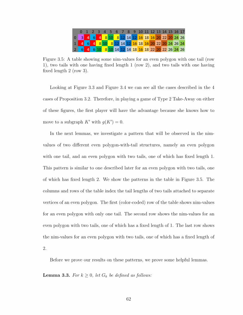
Figure 3.5: A table showing some nim-values for an even polygon with one tail (row1), two tails with one having fixed length 1 (row 2), and two tails with one havingfixed length 2 (row 3).
Looking at Figure 3.3 and Figure 3.4 we can see all the cases described in the 4
cases of Proposition 3.2. Therefore, in playing a game of Type 2 Take-Away on either
of these figures, the first player will have the advantage because she knows how to
move to a subgraph K ′ with g(K ′) = 0.
In the next lemmas, we investigate a pattern that will be observed in the nim-
values of two different even polygon-with-tail structures, namely an even polygon
with one tail, and an even polygon with two tails, one of which has fixed length 1.
This pattern is similar to one described later for an even polygon with two tails, one
of which has fixed length 2. We show the patterns in the table in Figure 3.5. The
columns and rows of the table index the tail lengths of two tails attached to separate
vertices of an even polygon. The first (color-coded) row of the table shows nim-values
for an even polygon with only one tail. The second row shows the nim-values for an
even polygon with two tails, one of which has a fixed length of 1. The last row shows
the nim-values for an even polygon with two tails, one of which has a fixed length of
2.
Before we prove our results on these patterns, we prove some helpful lemmas.
Lemma 3.3. For k ≥ 0, let Gk be defined as follows:
62

• If k ≡ 1 mod 3 then Gk = 4k+83
• If k ≡ 2 mod 3 then Gk = 4k+103
• If k ≡ 0 mod 3 then Gk = 4k3
If k ≡ 1 mod 3 then:
• Gk ⊕ 1 = 4k+113
• Gk ⊕ 2 = 4k+143
• Gk+1 ⊕ 1 = 4k+83
• Gk+1 ⊕ 2 = 4k+173
• Gk+2 ⊕ 1 = 4k+113
• Gk+2 ⊕ 2 = 4k+143
This forms a set of 4 consecutive integers, Sk = {Gk ⊕ 1, Gk ⊕ 2, Gk+1 ⊕
1, Gk+1 ⊕ 2, Gk+2 ⊕ 1, Gk+2 ⊕ 2} = {Gk ⊕ 1, Gk ⊕ 2, Gk+1 ⊕ 1, Gk+1 ⊕ 2} =
{4k+83, 4k+11
3, 4k+14
3, 4k+17
3}, the first of which is a multiple of four.
Proof. Let Gk be as described and assume k ≡ 1 mod 3.
First, k ≡ 1 mod 3, then k + 2 ≡ 0 mod 3, and hence so is 4k + 8 ≡ 0 mod 3.
Thus k+23
(and 4k+83
) is an integer.
Then Gk = 4k+83
= 4(k+2)3
, and we see that Gk is divisible by 4. Therefore Gk is
even and its binary representation ends in 00. So, by the rules of nim addition, the
binary representation of Gk ⊕ 1 will end in 01 and be equivalent to ordinary integer
63

addition: 4k+83
+ 1 = 4k+113
. Similarly, the binary representation of Gk ⊕ 2 will end in
10 and be equivalent to ordinary integer addition: 4k+83
+ 2 = 4k+143
.
Now Gk+1 = 4(k+1)+103
= 4k+143
= 2(2k+7)3
. So we see that 2k + 7 ≡ 0 mod 3 and
so 2k+73
is an odd integer. Thus Gk+1 is divisible by 2 but not divisible by 4, so
its binary representation ends in 10. Again, by the rules of nim addition, the binary
representation ofGk+1⊕1 will end in 11 and be equivalent to ordinary integer addition:
4k+143
+ 1 = 4k+173
. This will not be the case, however, for Gk+1 ⊕ 2. Under the rules
of nim addition, the binary representation of Gk+1 ⊕ 2 will end in 00 since we are
taking the nim-sum of two binary values which each end in 10. Therefore, here, the
nim-sum would actually be regular integer subtraction: Gk+1⊕ 2 = 4k+143− 2 = 4k+8
3.
Last, we see that Gk+2 = 4(k+2)3
= 4k+83
, which is exactly the same as our first
case.
So, we have the set Sk = {4k+83, 4k+11
3, 4k+14
3, 4k+17
3} which is {4k+8
3, 4k+8
3+1, 4k+8
3+
2, 4k+83
+3}, and hence a set of four consecutive integers, the first of which is a multiple
of four.
Lemma 3.4. For k ≥ 1 and k ≡ 1 mod 3, let Sk be a set defined as in Lemma 3.3.
Then S1 ∪ S4 ∪ · · · ∪ Sk = {4, 5, 6, 7, ..., 4k+83, 4k+11
3, 4k+14
3, 4k+17
3}.
Proof. By the definition of Sk, S1 = {4(1)+83
, 4(1)+113
, 4(1)+143
, 4(1)+173} = {4, 5, 6, 7}.
Similarly, S4 = {4(4)+83
, 4(4)+113
, 4(4)+143
, 4(4)+173} = {8, 9, 10, 11}. Then S1
⋃S4 =
{4, 5, 6, 7, 8, 9, 10, 11}.
Observe, in general, the highest integer in Sk−3 is 4k+53
and the lowest value in Sk
is 4k+83
= 4k+53
+ 1.
64

Note that while Lemma 3.3 involves nim-sum, neither Lemma 3.3 nor Lemma 3.4
relies on any particular game or structure.
Finally we are ready to begin proving results about Type 2 Take-Away on an even
polygon with a single tail.
Theorem 3.5. Let K be an even polygon with n vertices and a tail with length at
least 1 attached to exactly one vertex of the polygon. Then, in Type 2 Take-Away,
g(K) is determined by the length, `, of the tail. Specifically,
• If ` ≡ 1 mod 3 then g(K) = 4`+83
,
• If ` ≡ 2 mod 3 then g(K) = 4`+103
,
• If ` ≡ 0 mod 3 then g(K) = 4`3
.
Proof. Let K be as described. Let ` be the length of the tail. The proof is by
induction on `.
Base case: Let ` = 1. Proposition 3.2 tells us that we can move to positions
K ′ with g(K ′) = 0, 1, 2, and 3, and the proof tells us what to remove to reach the
position associated with each value. It is important to note that all of these moves
are made in a way that removes the polygonal face; either we remove the polygonal
face itself, one of its edges (hence taking the polygonal face), or one of its vertices
(taking the incident edges and the polygonal face with it.) The only moves that we
can make on K that are not on the polygon are to remove the end vertex of the tail
(taking the edge of the tail with it) or to remove the edge of the tail. If we remove the
former, we will be left with just the polygon, and this K ′ has g(K ′) = 3 (see Theorem
65

3.1). If we remove the latter, K ′ will be the polygon with an additional unattached
vertex, so we find the nim-value of K ′ via nim-sum and g(K ′) = 3 ⊕ 1 = 2. Hence,
by Definition 1.2, g(K) = 4, as desired.
Assume, then, that the statement is true for all even polygons with tail of length
j, 1 ≤ j ≤ `− 1. Consider an even polygon with tail of length `. We have three cases
to consider.
• Case 1: Suppose ` ≡ 1 mod 3. We have 4 types of moves to consider:
– Case 1a: Removing the polygonal face or a vertex or edge on the polygon
will result in a position K ′ which is a bipartite graph. Proposition 3.2
shows that we can arrive at positions with g(K ′) equal to 0, 1, 2, and 3 via
this type of move, and by the results for Take-Away on a bipartite graph
we will not arrive at a position with g(K ′) ≥ 4.
– Case 1b: Removing the vertex at the end of the tail, v, leaves a position
K ′ with a tail of length `− 1 and `− 1 ≡ 0 mod 3. By induction, g(K ′) =
4(`−1)3
= 4`−43
.
– Case 1c: Removing the vertex, u, which is on the tail and adjacent to
a vertex of the polygon, results in a position K ′ that consists of an even
polygon on n vertices and a disjoint path. Similarly, if we remove the edge
that is incident to the polygon vertex and to u, we will also result in a
position K ′ that consists of an even polygon on n vertices and a disjoint
path that is longer than the previous path by one edge. By Theorem 3.1,
we know that the even polygon has nim-value 3. A path is a bipartite
66

graph and will have nim-value 1 or 2. Since we find the nim-values here
using nim-sum and the path lengths differ by 1, one of these positions will
have g(K ′) = 3⊕ 1 = 2 and the other will have g(K ′) = 3⊕ 2 = 1.
– Case 1d: Removing any other vertex or edge from the tail leaves a position
K ′ which is an even polygon with a tail of length j, 1 ≤ j ≤ ` − 2, and
a disjoint path. A path is a bipartite graph and will have nim-value 1
or 2. By selectively removing a vertex—taking with it two edges—or a
single edge, it is possible to move to every combination of smaller polygon
with a shorter tail of length j, 1 ≤ j ≤ ` − 2 and a disjoint path; that
is, the nim-values will be found via nim-sum. So the results of Lemma
3.3 and Lemma 3.4 show us that we can get all nim-values from the set
{4, 5, ..., 4`+53}.
Since these are all the moves we can make, we conclude the nim-value is the
least integer that we cannot reach; therefore g(K) = 4`+53
+ 1 = 4`+83
.
• Case 2: Suppose ` ≡ 2 mod 3. We have 4 types of moves to consider:
– Case 2a: Removing the polygonal face or a vertex or edge on the polygon
will be to a position K ′ which is a bipartite graph. Proposition 3.2 shows
that we can arrive at positions with g(K ′) equal to 0, 1, 2, and 3 via this
type of move, and by the results for Take-Away on a bipartite graph we
will not arrive at a position with g(K ′) ≥ 4.
– Case 2b: Removing the vertex at the end of the tail, v, is a move to a
positionK ′ with tail length `−1, and by induction g(K ′) = 4(`−1)+83
= 4`+43
.
67

Removing the last edge of the tail but leaving v takes us to a position K ′
which has g(K ′) = 4`+43⊕ 1 = 4`+7
3.
– Case 2c: Removing the vertex, u, which is on the tail and adjacent to
a vertex of the polygon, results in a position K ′ that consists of an even
polygon on n vertices and a disjoint path. Similarly, if we remove the edge
that is incident to the polygon vertex and to u, we will also result in a
position K ′ that consists of an even polygon on n vertices and a disjoint
path that is longer than the previous path by one edge. By Theorem 3.1,
we know that the even polygon has nim-value 3. A path is a bipartite
graph and will have nim-value 1 or 2. Since we find the nim-values here
using nim-sum and the path lengths differ by 1, one of these positions will
have g(K ′) = 3⊕ 1 = 2 and the other will have g(K ′) = 3⊕ 2 = 1.
– Case 2d: Removing any other vertex or edge from the tail leaves a position
K ′ which is an even polygon with a tail of length j, 1 ≤ j ≤ ` − 2, and
a disjoint path. A path is a bipartite graph and will have nim-value 1
or 2. By selectively removing a vertex—taking with it two edges—or a
single edge, it is possible to move to every combination of smaller polygon
with a shorter tail of length j, 1 ≤ j ≤ ` − 2 and a disjoint path; that
is, the nim-values will be found via nim-sum. So the results of Lemma
3.3 and Lemma 3.4 show us that we can get all nim-values from the set
{4, 5, ..., 4`+13}.
Combining these values we see that the first unreachable integer is 4`+103
, and
68

therefore this is g(K).
• Case 3: Suppose ` ≡ 0 mod 3. We have 5 types of moves to consider:
– Case 3a: Removing the polygonal face or a vertex or edge on the polygon
will be to a position K ′ which is a bipartite graph. Proposition 3.2 shows
that we can arrive at positions with g(K ′) equal to 0, 1, 2, and 3 via this
type of move, and by the results for Take-Away on a bipartite graph we
will not arrive at a position with g(K ′) ≥ 4.
– Case 3b: Removing the end vertex, v, of the tail leaves a position K ′ with
g(K ′) = 4(`−1)+103
= 4`+63
. Removing the last edge of the tail but leaving v
yields a position K ′ with g(K ′) = 4`+63⊕ 1 = 4`+9
3.
– Case 3c: Removing the vertex, u, which is on the tail and adjacent to
a vertex of the polygon, results in a position K ′ that consists of an even
polygon on n vertices and a disjoint path. Similarly, if we remove the edge
that is incident to the polygon vertex and to u, we will also result in a
position K ′ that consists of an even polygon on n vertices and a disjoint
path that is longer than the previous path by one edge. By Theorem 3.1,
we know that the even polygon has nim-value 3. A path is a bipartite
graph and will have nim-value 1 or 2. Since we find the nim-values here
using nim-sum and the path lengths differ by 1, one of these positions will
have g(K ′) = 3⊕ 1 = 2 and the other will have g(K ′) = 3⊕ 2 = 1.
– Case 3d: Removing the vertex in the tail adjacent to v, say w, leaves a
position K ′ with a polygon and shorter tail which has nim-value 4(`−2)+83
=
69
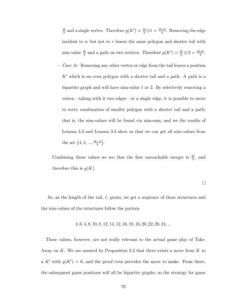
4`3
and a single vertex. Therefore g(K ′) = 4`3⊕1 = 4`+3
3. Removing the edge
incident to w but not to v leaves the same polygon and shorter tail with
nim-value 4`3
and a path on two vertices. Therefore g(K ′) = 4`3⊕ 2 = 4`+6
3.
– Case 3e: Removing any other vertex or edge from the tail leaves a position
K ′ which is an even polygon with a shorter tail and a path. A path is a
bipartite graph and will have nim-value 1 or 2. By selectively removing a
vertex—taking with it two edges—or a single edge, it is possible to move
to every combination of smaller polygon with a shorter tail and a path;
that is, the nim-values will be found via nim-sum, and we the results of
Lemma 3.3 and Lemma 3.4 show us that we can get all nim-values from
the set {4, 5, ..., 4`−33}.
Combining these values we see that the first unreachable integer is 4`3
, and
therefore this is g(K).
So, as the length of the tail, `, grows, we get a sequence of these structures and
the nim-values of the structures follow the pattern
4, 6, 4, 8, 10, 8, 12, 14, 12, 16, 18, 16, 20, 22, 20, 24, ...
. These values, however, are not really relevant to the actual game play of Take-
Away on K. We are assured by Proposition 3.2 that there exists a move from K to
a K ′ with g(K ′) = 0, and the proof even provides the move to make. From there,
the subsequent game positions will all be bipartite graphs, so the strategy for game
70

play is known. However, we recall that the motivation for studying this particular
structure was to build up from here to eventually understand and find a winning
strategy for playing Type 2 Take-Away on a grid or tiling of the plane. Further, if
we borrow a cue from multi-heap nim and begin a game with multiple polygons with
single tails then the nim-values become very important for determining the strategy
for play.
3.3 Even Polygons with Two Tails
The next step, then, is to add another tail to the polygon. In the following theorems
we will show that nim-values of these structures are also easily determined, something
we can see from the table of partial values introduced earlier in Figure 3.5.
Theorem 3.6. Let T be an even polygon with n vertices and two tails, each adjacent
to a separate vertex on the polygon. Suppose one of those tails has length 1. Then,
in Type 2 Take-Away, g(T ) is determined by the combined length, t, of the two tails.
Specifically,
• If t ≡ 1 mod 3 then g(T ) = 4t+83
• If t ≡ 2 mod 3 then g(T ) = 4t+103
• If t ≡ 0 mod 3 then g(T ) = 4t3
Proof. Let T be as described. Let t be the combined length of the tails. The proof is
by induction on t.
71

Base Cases: Let T be an even polygon with two tails. Suppose one tail has length
1 and the other tail has length 0. Then the combined tail length, t, is 1. By Theorem
3.5 we know this structure has g(T ) = 4.
Now, let T be an even polygon with two tails attached, each to a different vertex
of the polygon. Let each tail have length 1 so that lt = 2. By Proposition 3.2, we
know that it is possible to reach positions T ′ through one move that have g(T ′) = 0,
1, 2, and 3. Recall that these values are reached by removing particular components
from the polygon, whether it be the polygonal face itself, or an edge or a vertex from
around the polygon. Let’s consider the nim-values of the other positions that it is
possible to reach through one move. Removing the end vertex, v, from one of the
tails will result in an even polygon with one tail which has length 1. By Theorem
3.5 we know this structure has g(T ′) = 4. Alternatively, we could remove the edge
incident to both v and the polygon; this results in a T ′ with an even polygon with
one tail of length 1 and also a disconnected vertex. We must use the nim-sum to find
the nim-value, and g(T ′) = 4⊕1 = 5. Hence, by Definition 1.2 we find that g(T ) = 6.
Now, assume that the statement is true for all k, 1 ≤ k ≤ t − 1 and let T be an
even polygon with two tails, one of fixed lengh 1, and the total tail length be t. Let
us consider the positions we can reach from T through just one move.
• Case 1: Suppose t ≡ 1 mod 3. We have 5 types of moves to consider:
– Case 1a: Removing the polygonal face or a vertex or edge on the polygon
will be to a position T ′ which is a bipartite graph. Proposition 3.2 shows
that we can arrive at positions with g(T ′) equal to 0, 1, 2, and 3 via this
72

type of move, and by the results for Take-Away on a bipartite graph we
will not arrive at a position with g(T ′) ≥ 4.
– Case 1b: Removing the vertex at the end of the tail of length 1, v, leaves
a position T ′ with a single tail of length t − 1 and t − 1 ≡ 0 mod 3. By
Theorem 3.5, g(T ′) = 4(t−1)3
= 4t−43
. Removing the edge incident to v leaves
a position with the aforementioned T ′ plus a disjoint vertex. Through nim-
sum, we find the nim-value of this position to be 4t−43⊕ 1 = 4t+7
3.
– Case 1c: Removing the vertex, u, that is on the tail of length t− 1 that is
adjacent to a vertex on the polygon results in a position T ′ which has an
even polygon with a single tail of length 1 and a disjoint path. Removing
the edge incident to both u and the polygon results in a position T ′ which
has an even polygon with a single tail of length 1 and a disjoint path that is
longer than the previous path by one edge. A path is a bipartite graph and
will have nim-value 1 or 2. The even polygon with a single tail of length
1 has nim-value 4 (see Theorem 3.5). So, between these two positions we
will have a move so that we can get to g(T ′) = 4 ⊕ 1 = 5 and a move so
that we can get to g(T ′) = 4⊕ 2 = 6.
– Case 1d: Removing the end vertex from the tail of length t− 1 results in
a position T ′ that, by induction, has g(T ′) = 4t−43
.
– Case 1e: Removing any other vertex or edge from the tail of length t− 1
leaves a position T ′ which can have two components: a polygon with two
tails, one with fixed length 1, but with a total tail length t′, 1 ≤ t′ ≤ t− 1
73
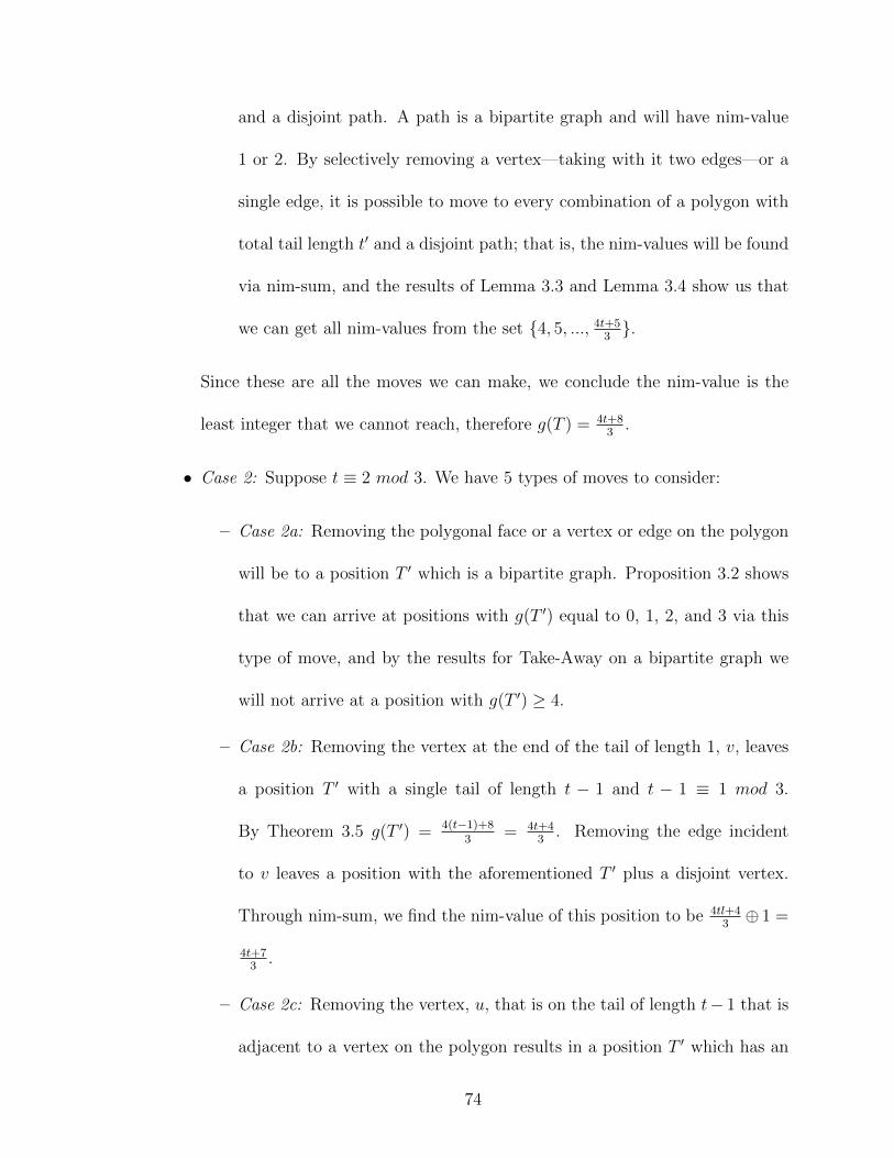
and a disjoint path. A path is a bipartite graph and will have nim-value
1 or 2. By selectively removing a vertex—taking with it two edges—or a
single edge, it is possible to move to every combination of a polygon with
total tail length t′ and a disjoint path; that is, the nim-values will be found
via nim-sum, and the results of Lemma 3.3 and Lemma 3.4 show us that
we can get all nim-values from the set {4, 5, ..., 4t+53}.
Since these are all the moves we can make, we conclude the nim-value is the
least integer that we cannot reach, therefore g(T ) = 4t+83
.
• Case 2: Suppose t ≡ 2 mod 3. We have 5 types of moves to consider:
– Case 2a: Removing the polygonal face or a vertex or edge on the polygon
will be to a position T ′ which is a bipartite graph. Proposition 3.2 shows
that we can arrive at positions with g(T ′) equal to 0, 1, 2, and 3 via this
type of move, and by the results for Take-Away on a bipartite graph we
will not arrive at a position with g(T ′) ≥ 4.
– Case 2b: Removing the vertex at the end of the tail of length 1, v, leaves
a position T ′ with a single tail of length t − 1 and t − 1 ≡ 1 mod 3.
By Theorem 3.5 g(T ′) = 4(t−1)+83
= 4t+43
. Removing the edge incident
to v leaves a position with the aforementioned T ′ plus a disjoint vertex.
Through nim-sum, we find the nim-value of this position to be 4tl+43⊕ 1 =
4t+73
.
– Case 2c: Removing the vertex, u, that is on the tail of length t− 1 that is
adjacent to a vertex on the polygon results in a position T ′ which has an
74

even polygon with a single tail of length 1 and a disjoint path. Removing
the edge incident to both u and the polygon results in a position T ′ which
has an even polygon with a single tail of length 1 and a disjoint path that is
longer than the previous path by one edge. A path is a bipartite graph and
will have nim-value 1 or 2. The even polygon with a single tail of length
1 has nim-value 4 (see Theorem 3.5). So, between these two positions we
will have a move so that we can get to g(T ′) = 4 ⊕ 1 = 5 and a move so
that we can get to g(T ′) = 4⊕ 2 = 6.
– Case 2d: Removing the end vertex from the tail of length t− 1 results in
a position T ′ that, by induction, has g(T ′) = 4(t−1)+83
= 4t+43
.
– Case 2e: Removing any other vertex or edge from the tail of length t− 1
leaves a position T ′ which can have two components:a polygon with two
tails, one with fixed length 1, but with a total tail length t′, 1 ≤ t′ ≤ t− 1
and a disjoint path. A path is a bipartite graph and will have nim-value
1 or 2. By selectively removing a vertex—taking with it two edges—or a
single edge, it is possible to move to every combination of a polygon with
total tail length t′ and a disjoint path; that is, the nim-values will be found
via nim-sum, and the results of Lemma 3.3 and Lemma 3.4 show us that
we can get all nim-values from the set {4, 5, ..., 4t+13}.
Combining these values we see that the first unreachable integer is 4t+103
, and
therefore this is g(T ).
• Case 3: Suppose t ≡ 0 mod 3. We have 4 types of moves to consider:
75

– Case 3a: Removing the polygonal face or a vertex or edge on the polygon
will be to a position T ′ which is a bipartite graph. Proposition 3.2 shows
that we can arrive at positions with g(T ′) equal to 0, 1, 2, and 3 via this
type of move, and by the results for Take-Away on a bipartite graph we
will not arrive at a position with g(T ′) ≥ 4.
– Case 3b: Removing the end vertex, v, of the tail of length 1 leaves a
position T ′ with g(T ′) = 4(t−1)+103
= 4t+63
. Removing the edge of the tail
adjacent to v yields a position T ′ with g(T ′) = 4t+63⊕ 1 = 4t+9
3.
– Case 3c: Removing the vertex, u, that is on the tail of length t− 1 that is
adjacent to a vertex on the polygon results in a position T ′ which has an
even polygon with a single tail of length 1 and a disjoint path. Removing
the edge incident to both u and the polygon results in a position T ′ which
has an even polygon with a single tail of length 1 and a disjoint path that is
longer than the previous path by one edge. A path is a bipartite graph and
will have nim-value 1 or 2. The even polygon with a single tail of length
1 has nim-value 4 (see Theorem 3.5). So, between these two positions we
will have a move so that we can get to g(T ′) = 4 ⊕ 1 = 5 and a move so
that we can get to g(T ′) = 4⊕ 2 = 6.
– Case 3d: Removing the end vertex, w, of the other tail results in a position
T ′ with a polygon and total tail length t−1 which, by induction, has nim-
value 4(t−1)+103
= 4t+63
. Removing the edge of the tail adjacent to w yields
a position T ′ with g(T ′) = 4t+63⊕ 1 = 4t+9
3.
76

– Case 3e: Removing any other vertex or edge from the tail of length t− 1
leaves a position T ′which can have two components:a polygon with two
tails, one with fixed length 1, but with a total tail length t′, 1 ≤ t′ ≤ t− 1
and a disjoint path. A path is a bipartite graph and will have nim-value
1 or 2. By selectively removing a vertex—taking with it two edges—or a
single edge, it is possible to move to every combination of a polygon with
total tail length t′ and a disjoint path; that is, the nim-values will be found
via nim-sum, and the results of Lemma 3.3 and Lemma 3.4 show us that
we can get all nim-values from the set {4, 5, ..., 4t−33}.
Combining these values we see that the first unreachable integer is 4t3
, and
therefore this is g(T ).
Our next result is for an even polygonal tile with two attached tails, one of which
has a fixed length of 2. Just as the previous results about an even polygon with one
tail and an even polygon with two tails, one of length 1, there is an easily described
pattern to the nim-values of these structures when playing Type 2 Take-Away. While
this pattern follows a very similar structure, it is not the same pattern, hence we
prove Lemmas similar to Lemma 3.3 and Lemma 3.4 to reflect the new pattern we
see here.
Lemma 3.7. Let Gk be defined as follows:
• If k ≡ 0 mod 3 then Gk = 4k+183
77

• If k ≡ 1 mod 3 then Gk = 4k+83
• If k ≡ 2 mod 3 then Gk = 4k+103
If k ≡ 0 mod 3 then:
• Gk ⊕ 1 = 4k+213
• Gk ⊕ 2 = 4k+123
• Gk+1 ⊕ 1 = 4k+153
• Gk+1 ⊕ 2 = 4k+183
• Gk+2 ⊕ 1 = 4k+213
• Gk+2 ⊕ 2 = 4k+123
This forms a set of 4 consecutive integers, Sk = {4k+123
, 4k+153
, 4k+183
, 4k+213}, the first
of which is a multiple of four.
Proof. Let Gk be as described and assume k ≡ 0 mod 3.
First, we know that 4k+183
is an integer because if k ≡ 0 mod 3 then 4k ≡ 0 mod 3
and since 18 ≡ 0 mod 3, 4k + 18 ≡ 0 mod 3. This means that 4k + 18 is divisible by
3, hence 4k+183
is an integer.
Then Gk = 4k+183
= 2(2k+9)3
, and we see that Gk is divisible by 2 but is not divisible
by 4. Therefore Gk is even and its binary representation ends in 10. So, by the rules
of nim addition, the binary representation of Gk ⊕ 1 will end in 01 and be equivalent
to regular integer addition: 4k+183
+ 1 = 4k+213
. This will not be the case, however, for
78

Gk⊕ 2. Under the rules of nim addition, the binary representation of Gk⊕ 2 will end
in 00 since we are adding two binary values which each end in 10. Therefore, here,
the nim-sum would actually be regular integer subtraction: 4k+183− 2 = 4k+12
3.
Now Gk+1 = 4(k+1)+83
= 4k+123
= 4(k+3)3
. So we see that Gk+1 is divisible by 4, so
its binary representation ends in 00. Again, by the rules of nim addition, the binary
representation of Gk+1⊕1 will end in 01 and be equivalent to regular integer addition:
4k+123
+ 1 = 4k+153
. Similarly, Gk+1 ⊕ 2 = 4k+123
+ 2 = 4k+183
.
Last, we see that Gk+2 = 4(k+2)+103
= 4k+183
, which is exactly the same as our first
case.
So, we have the set Sk = {4k+123
, 4k+153
, 4k+183
, 4k+213} which is {4k+12
3, 4k+12
3+
1, 4k+123
+ 2, 4k+123
+ 3}, and hence a set of four consecutive integers, the first of
which is a multiple of four.
Lemma 3.8. Let Sk be a set defined as in Lemma 3.7. Then S1
⋃S4
⋃...⋃Sk =
{4, 5, 6, 7, ..., 4k+123
, 4k+153
, 4k+183
, 4k+213}.
Proof. By the definition of Sk, S1 = {4(0)+123
, 4(0)+153
, 4(0)+183
, 4(0)+213} = {4, 5, 6, 7}.
Similarly, S4 = {4(3)+123
, 4(3)+153
, 4(3)+183
, 4(3)+213} = {8, 9, 10, 11}. Then S1
⋃S4 =
{4, 5, 6, 7, 8, 9, 10, 11}.
Observe, in general, the highest integer in Sk−3 is 4k+53
and he lowest value in Sk
is 4k+83
= 4k+53
+ 1.
With these lemmas, we can now prove the result about the pattern found in the
nim-values of an even polygons with two tails, each connected to a separate vertex
on the polygon.
79
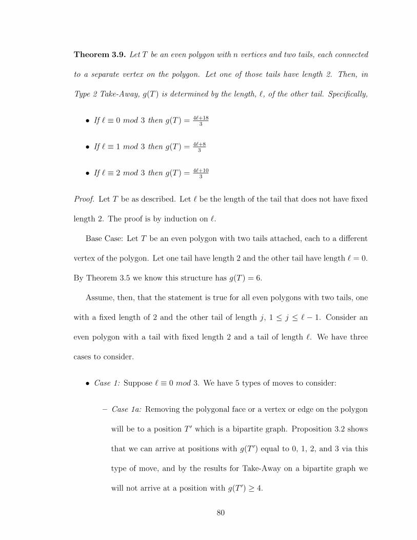
Theorem 3.9. Let T be an even polygon with n vertices and two tails, each connected
to a separate vertex on the polygon. Let one of those tails have length 2. Then, in
Type 2 Take-Away, g(T ) is determined by the length, `, of the other tail. Specifically,
• If ` ≡ 0 mod 3 then g(T ) = 4`+183
• If ` ≡ 1 mod 3 then g(T ) = 4`+83
• If ` ≡ 2 mod 3 then g(T ) = 4`+103
Proof. Let T be as described. Let ` be the length of the tail that does not have fixed
length 2. The proof is by induction on `.
Base Case: Let T be an even polygon with two tails attached, each to a different
vertex of the polygon. Let one tail have length 2 and the other tail have length ` = 0.
By Theorem 3.5 we know this structure has g(T ) = 6.
Assume, then, that the statement is true for all even polygons with two tails, one
with a fixed length of 2 and the other tail of length j, 1 ≤ j ≤ ` − 1. Consider an
even polygon with a tail with fixed length 2 and a tail of length `. We have three
cases to consider.
• Case 1: Suppose ` ≡ 0 mod 3. We have 5 types of moves to consider:
– Case 1a: Removing the polygonal face or a vertex or edge on the polygon
will be to a position T ′ which is a bipartite graph. Proposition 3.2 shows
that we can arrive at positions with g(T ′) equal to 0, 1, 2, and 3 via this
type of move, and by the results for Take-Away on a bipartite graph we
will not arrive at a position with g(T ′) ≥ 4.
80
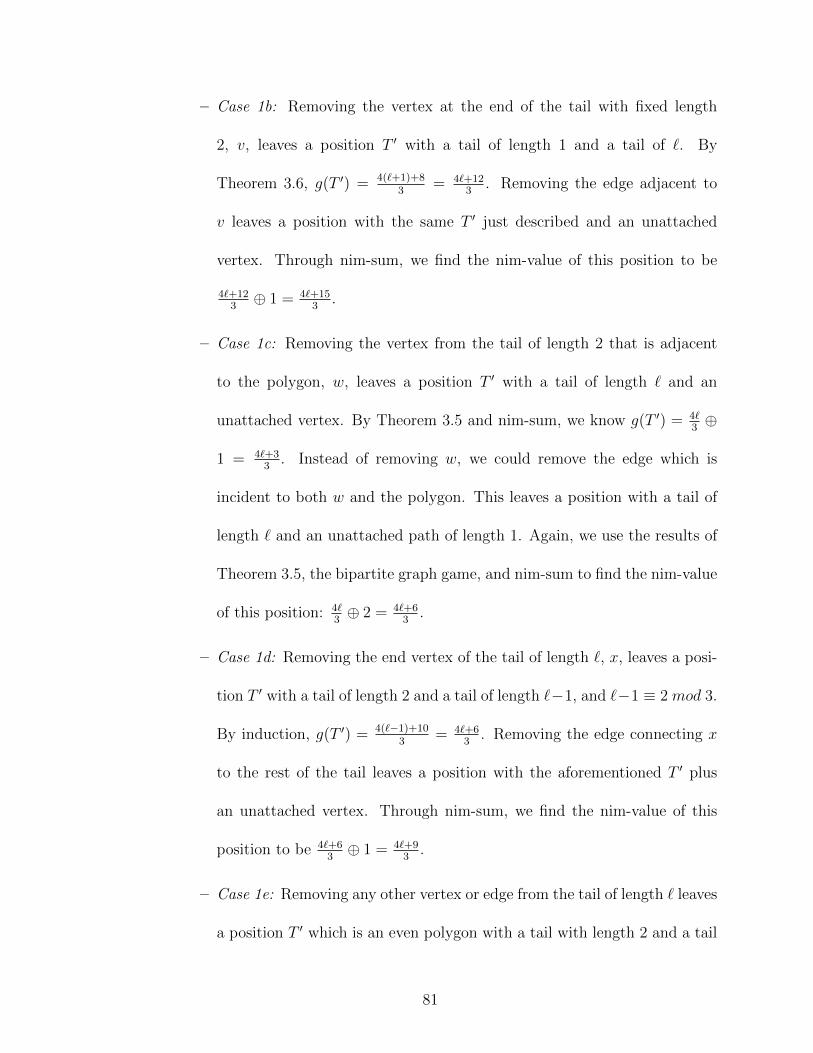
– Case 1b: Removing the vertex at the end of the tail with fixed length
2, v, leaves a position T ′ with a tail of length 1 and a tail of `. By
Theorem 3.6, g(T ′) = 4(`+1)+83
= 4`+123
. Removing the edge adjacent to
v leaves a position with the same T ′ just described and an unattached
vertex. Through nim-sum, we find the nim-value of this position to be
4`+123⊕ 1 = 4`+15
3.
– Case 1c: Removing the vertex from the tail of length 2 that is adjacent
to the polygon, w, leaves a position T ′ with a tail of length ` and an
unattached vertex. By Theorem 3.5 and nim-sum, we know g(T ′) = 4`3⊕
1 = 4`+33
. Instead of removing w, we could remove the edge which is
incident to both w and the polygon. This leaves a position with a tail of
length ` and an unattached path of length 1. Again, we use the results of
Theorem 3.5, the bipartite graph game, and nim-sum to find the nim-value
of this position: 4`3⊕ 2 = 4`+6
3.
– Case 1d: Removing the end vertex of the tail of length `, x, leaves a posi-
tion T ′ with a tail of length 2 and a tail of length `−1, and `−1 ≡ 2 mod 3.
By induction, g(T ′) = 4(`−1)+103
= 4`+63
. Removing the edge connecting x
to the rest of the tail leaves a position with the aforementioned T ′ plus
an unattached vertex. Through nim-sum, we find the nim-value of this
position to be 4`+63⊕ 1 = 4`+9
3.
– Case 1e: Removing any other vertex or edge from the tail of length ` leaves
a position T ′ which is an even polygon with a tail with length 2 and a tail
81

with length j ≤ ` and an unattached path. A path is a bipartite graph and
will have nim-value 1 or 2. By selectively removing a vertex—taking with
it two edges—or a single edge, it is possible to move to every combination
of such a structure and a path; that is, the nim-values will be found via
nim-sum, and the results of Lemma 3.7 and Lemma 3.8 show us that we
can get all nim-values from the set {4, 5, ..., 4`+93}.
Since these are all the moves we can make, we conclude the nim-value is the
least integer that we cannot reach, therefore g(K) = 4`+183
.
• Case 2: Suppose ` ≡ 1 mod 3. We have 5 types of moves to consider:
– Case 2a: Removing the polygonal face or a vertex or edge on the polygon
will be to a position T ′ which is a bipartite graph. Proposition 3.2 shows
that we can arrive at positions with g(T ′) equal to 0, 1, 2, and 3 via this
type of move, and by the results for Take-Away on a bipartite graph we
will not arrive at a position with g(T ′) ≥ 4.
– Case 2b: Removing the vertex at the end of the tail with fixed length
2, v, leaves a position T ′ with a tail of length 1 and a tail of `. By
Theorem 3.6, g(T ′) = 4(`+1)+103
= 4`+143
. Removing the edge adjacent to
v leaves a position with the same T ′ just described and an unattached
vertex. Through nim-sum, we find the nim-value of this position to be
4`+143⊕ 1 = 4`+17
3.
– Case 2c: Removing the vertex from the tail of length 2 that is adjacent to
the polygon, w, leaves a posiion T ′ with a tail of length ` and an unattached
82

vertex. By Theorem 3.5 and nim-sum, we know g(T ′) = 4`+83⊕ 1 = 4`+11
3.
Instead of removing w, we could remove the edge which is incident to both
w and the polygon. This leaves a position with a tail of length ` and an
unattached path of length 1. Again, we use the results of Theorem 3.5, the
bipartite graph game, and nim-sum to find the nim-value of this position:
4`+83⊕ 2 = 4`+14
3.
– Case 2d: Removing the end vertex of the tail of length `, x, leaves a posi-
tion T ′ with a tail of length 2 and a tail of length `−1, and `−1 ≡ 0 mod 3.
By induction, g(T ′) = 4(`−1)+183
= 4`+143
. Removing the edge connecting
x to the rest of the tail leaves a position with the aforementioned T ′ plus
an unattached vertex. Through nim-sum, we find the nim-value of this
position to be 4`+143⊕ 1 = 4`+17
3.
– Case 2e: Removing any other vertex or edge from the tail of length ` leaves
a position T ′ which is an even polygon with a tail with length 2 and a tail
with length j ≤ ` and an unattached path. A path is a bipartite graph and
will have nim-value 1 or 2. By selectively removing a vertex—taking with
it two edges—or a single edge, it is possible to move to every combination
of such a structure and a path; that is, the nim-values will be found via
nim-sum, and the results of Lemma 3.7 and Lemma 3.8 show us that we
can get all nim-values from the set {4, 5, ..., 4`+53}.
Combining these values we see that the first unreachable integer is 4`+83
, and
therefore this is g(T ).
83

• Case 3: Suppose ` ≡ 2 mod 3. We have 5 types of moves to consider:
– Case 3a: Removing the polygonal face or a vertex or edge on the polygon
will be to a position T ′ which is a bipartite graph. Proposition 3.2 shows
that we can arrive at positions with g(T ′) equal to 0, 1, 2, and 3 via this
type of move, and by the results for Take-Away on a bipartite graph we
will not arrive at a position with g(T ′) ≥ 4.
– Case 3b: Removing the vertex at the end of the tail with fixed length 2, v,
leaves a position T ′ with a tail of length 1 and a tail of `. By Theorem 3.6,
g(T ′) = 4(`+1)3
= 4`+43
. Removing the edge adjacent to v leaves a position
with the same T ′ just described and an unattached vertex. Through nim-
sum, we find the nim-value of this position to be 4`+43⊕ 1 = 4`+7
3.
– Case 3c: Removing the vertex from the tail of length 2 that is adjacent
to the polygon, w, leaves a position T ′ with a tail of length ` and an
unattached vertex. By Theorem 3.5 and nim-sum, we know g(T ′) = 4`+103⊕
1 = 4`+133
. Instead of removing w, we could remove the edge which is
incident to both w and the polygon. This leaves a position with a tail of
length ` and an unattached path of length 1. Again, we use the results of
Theorem 3.5, the bipartite graph game, and nim-sum to find the nim-value
of this position: 4`+103⊕ 2 = 4`+16
3.
– Case 3d: Removing the end vertex of the tail of length `, x, leaves a posi-
tion T ′ with a tail of length 2 and a tail of length `−1, and `−1 ≡ 1 mod 3.
By induction, g(T ′) = 4(`−1)+83
= 4`+43
. Removing the edge connecting x
84

to the rest of the tail leaves a position with the aforementioned T ′ plus
an unattached vertex. Through nim-sum, we find the nim-value of this
position to be 4`+43⊕ 1 = 4`+7
3.
– Case 3e: Removing any other vertex or edge from the tail of length ` leaves
a position T ′ which is an even polygon with a tail with length 2 and a tail
with length j ≤ ` and an unattached path. A path is a bipartite graph and
will have nim-value 1 or 2. By selectively removing a vertex—taking with
it two edges—or a single edge, it is possible to move to every combination
of such a structure and a path; that is, the nim-values will be found via
nim-sum, and the results of Lemma 3.7 and Lemma 3.8 show us that we
can get all nim-values from the set {4, 5, ..., 4`+53}.
Combining these values we see that the first unreachable integer is 4`+103
, and
therefore this is g(K).
The nim-values we have seen here are always even and follow easily describable
patterns but are unbounded. That is, if we wanted a structure that has a nim-value
of 2k for any k ∈ N, k ≥ 3, then we could easily create it based on these theorems.
It is because of this that the next result is particularly interesting; we now continue
to look at an even polygon with two attached tails, but this time we consider the
length of both tails to be at least 3. What we find under this condition is that the
nim-values not only remain easy to determine based on tail length, but now they are
bounded.
85

Theorem 3.10. Let T be an even polygon with n vertices and two tails, each con-
nected to a separate vertex on the polygon. Let both of those tails have length at least
3. Then, in Type 2 Take-Away, g(T ) is determined by the combined length, `t, of the
two tails. Specifically,
• If `t is even then g(T ) = 4
• If `t is odd then g(T ) = 7.
Proof. Let T be as described. By Proposition 3.2, we know that it is possible to reach
positions through one move that have nim-values of 0, 1, 2, and 3 by removing the
polygonal face or an edge or vertex incident to it. Let’s consider the nim-values of
the other positions that are reachable through one move.
• A player could remove a vertex or edge that completely disconnects one tail
from T . The position now has two components, one is a tree and the other is
a polygon with a single tail as in Theorem 3.5; we will call this component K.
From this same theorem we know that g(K) will be determined by the length of
the remaining connected tail, and, since the tail is at least length 3, the smallest
possible g(K) is 8. The tree, of course, will have a nim-value of either 1 or 2.
When we use nim-sum to find the nim-value of our current position, we see that
there is no way to get a value smaller than 10⊕ 2 = 8.
• A player could remove a vertex or edge that leaves one tail from T with length 1.
The position now has two components, one is a tree and the other is a polygon
with two tails, one which has length 1, as in Theorem 3.6; we will call this
86
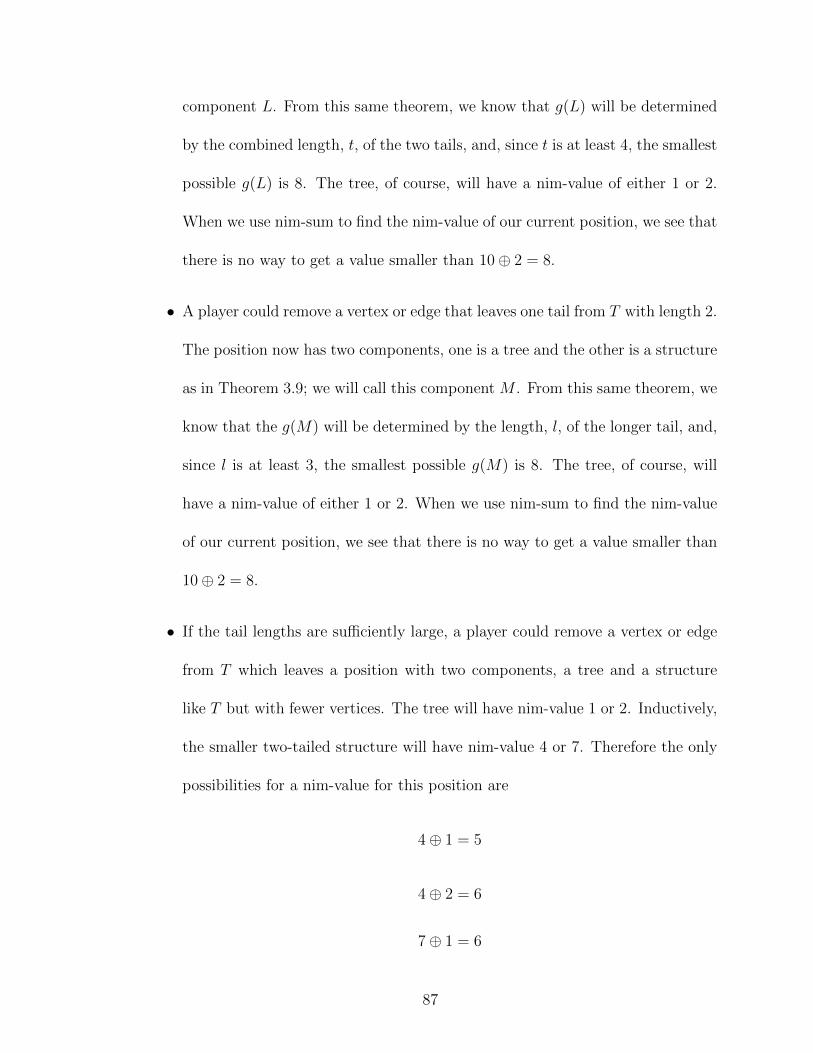
component L. From this same theorem, we know that g(L) will be determined
by the combined length, t, of the two tails, and, since t is at least 4, the smallest
possible g(L) is 8. The tree, of course, will have a nim-value of either 1 or 2.
When we use nim-sum to find the nim-value of our current position, we see that
there is no way to get a value smaller than 10⊕ 2 = 8.
• A player could remove a vertex or edge that leaves one tail from T with length 2.
The position now has two components, one is a tree and the other is a structure
as in Theorem 3.9; we will call this component M . From this same theorem, we
know that the g(M) will be determined by the length, l, of the longer tail, and,
since l is at least 3, the smallest possible g(M) is 8. The tree, of course, will
have a nim-value of either 1 or 2. When we use nim-sum to find the nim-value
of our current position, we see that there is no way to get a value smaller than
10⊕ 2 = 8.
• If the tail lengths are sufficiently large, a player could remove a vertex or edge
from T which leaves a position with two components, a tree and a structure
like T but with fewer vertices. The tree will have nim-value 1 or 2. Inductively,
the smaller two-tailed structure will have nim-value 4 or 7. Therefore the only
possibilities for a nim-value for this position are
4⊕ 1 = 5
4⊕ 2 = 6
7⊕ 1 = 6
87

7⊕ 2 = 5
.
• Lastly, for tails of sufficient length, a player could move an end edge or end
vertex from one of the tails of T . If the sum of the tail lengths of T is even,
removing the end vertex from one tail will move to a position with a similar
structure and a tail length sum which is odd, so inductively this position has
nim-value 7. If, instead, the player removes just the last edge, we have the same
structure with nim-value 7 and an isolated vertex, and under Nim sum this is a
position with nim-value 6. If the sum of the tail lengths of T is odd, removing
the end vertex from one tail will move to a position with a similar structure
and a tail length sum which is even, so inductively this position has nim-value
4. If, instead, the player removes just the last edge, we have the same structure
with nim-value 4 and an isolated vertex, and under Nim sum this is a position
with nim-value 5.
This analysis shows that if `t is even, it is impossible to move to a position with
nim-value 4, so the nim-value of T is 4. Similarly, if `t is odd, it is impossible to move
to a position with nim-value 7, so the nim-value of T is 7.
With these three theorems in mind, we find that the case of one even polygon
with two tails is completely solved, and in most cases is quite well-behaved.
88

Figure 3.6: An even polygon with tails connected to each of three vertices.
3.4 Even Polygons with Three Tails
In the previous section we found that an even polygon with two connected tails was
able to be completely solved with respect to finding nim-values of these structures in
a game of Type 2 Take-Away. The next step in our analysis is to add another tail to
the polygon. In Figure 3.6 we see an example of an even polygon with 3 tails.
It would be exciting to see results for an even polygon with three tails similar to
what we saw for even polygons with 1 and 2 tails. Unfortunately, though, the figures
that follow show that this is not the case. What we see in Figures 3.7 through 3.24
are tables of nim-values for even polygons with three tails. In each case, we hold the
length of one tail constant, and the table shows some of the nim-values as the other
tail lengths vary. Each particular number is given a unique color, and because of this
when we look at the tables we can see that there are many interesting patterns in
the three tail data, but describing them with a formula or a simple sentence like our
previous lemmas does not seem obvious.
Some of the observed patterns include:
• When the fixed length tail is of length n, if another tail also has length n then
as the third tail varies it follows the 4, 6, 4, 8, 10, 8, ... pattern we saw in
89

Figure 3.7: A table showing the nim-values for an even polygon with three tails, onehaving fixed length 0.
Theorem 3.5.
• Let the fixed length tail be of length n. If n ≡ 0 mod 3 then the table for a
tail of fixed length n is almost identical to the table for a tail with fixed length
n+ 2 and the table for a tail of fixed length n+ 1 is related in a noticeable way.
• Values mostly repeat in blocks of 9 values down the main diagonal of the table
for any fixed length n.
• If the tail lengths are sufficiently large and sufficiently far apart then it appears
the nim-value of the position will be 4 or 7.
There could very well be additional patterns in this data, and patterns that could
be easily proved, but at this time we have chosen not to focus on this task.
90

Figure 3.8: A table showing the nim-values for an even polygon with three tails, onehaving fixed length 1.
Figure 3.9: A table showing the nim-values for an even polygon with three tails, onehaving fixed length 2.
91

Figure 3.10: A table showing the nim-values for an even polygon with three tails, onehaving fixed length 3.
Figure 3.11: A table showing the nim-values for an even polygon with three tails, onehaving fixed length 4.
92

Figure 3.12: A table showing the nim-values for an even polygon with three tails, onehaving fixed length 5.
Figure 3.13: A table showing the nim-values for an even polygon with three tails, onehaving fixed length 6.
93

Figure 3.14: A table showing the nim-values for an even polygon with three tails, onehaving fixed length 7.
Figure 3.15: A table showing the nim-values for an even polygon with three tails, onehaving fixed length 8.
94

Figure 3.16: A table showing the nim-values for an even polygon with three tails, onehaving fixed length 9.
Figure 3.17: A table showing the nim-values for an even polygon with three tails, onehaving fixed length 10.
95

Figure 3.18: A table showing the nim-values for an even polygon with three tails, onehaving fixed length 11.
Figure 3.19: A table showing the nim-values for an even polygon with three tails, onehaving fixed length 12.
96

Figure 3.20: A table showing the nim-values for an even polygon with three tails, onehaving fixed length 13.
Figure 3.21: A table showing the nim-values for an even polygon with three tails, onehaving fixed length 14.
97

Figure 3.22: A table showing the nim-values for an even polygon with three tails, onehaving fixed length 15.
Figure 3.23: A table showing the nim-values for an even polygon with three tails, onehaving fixed length 16.
98

Figure 3.24: A table showing the nim-values for an even polygon with three tails, onehaving fixed length 17.
99

Figure 3.25: A quadrilateral with a tail connected to every vertex.
Figure 3.26: A quadrilateral with a tail connected to every vertex and all the movesthat can be made from that position in a game of Type 2 Take-Away. The nim-valueof each position is also included.
3.5 Quadrilaterals with Four Tails
After all of the interesting behavior we see for an even polygon with three tails, it is
somewhat surprising to find that it is possible for the nim-values to settle back down
and become easily describable again. When examining the case of a quadrilateral with
4 tails of any (non-zero) length, we find that the nim-values are very well-behaved.
Theorem 3.11. For a quadrilateral with a tail of nonzero length connected to every
100

vertex, Q, g(Q) is determined by the total number of vertices. Specifically,
• If |V (Q)| is even then g(Q) = 1
• If |V (Q)| is odd then g(Q) = 2.
Proof. Let Q be a quadrilateral with a nonempty tail connected to every vertex. The
proof is by induction on n, the number of vertices of Q.
Base case: Let Q be a quadrilateral with a tail of length 1 connected to every
vertex as in the top of Figure 3.26. In that figure we see every position that can
be reached from Q in one move of the game of Type 2 Take-Away. Based on this
analysis and the definition of nim-value, we find that g(Q) = 1.
Now, consider all the possible positions that could be achieved after one move in
the game of Type 2 Take-Away:
• Case 1: You could remove the polygonal face and move to a position that is a
bipartite graph with an equal number of vertices and edges; this position will
have either nim-value 0 or 3 depending on whether the number of vertices and
edges are both even or both odd, respectively.
• Case 2: You could remove a vertex adjacent to the quadrilateral, which will
also remove the quadrilateral and 3 total edges. This will reduce the number
of vertices by 1 and the number of edges by 3, so the total number of vertices
and edges will still have the same parity, either both even or both odd. This
position, then, would have nim-value 3 or 0, depending on whether Q initially
101

had an even number of both vertices and edges or an odd number of both
vertices and edges, respectively.
• Case 3: Removing an end vertex from one of the tails will move to a position
which looks like a smaller quadrilateral with 4 tails, and will have one less vertex
than Q and one less edge than Q . Inductively, the nim-value of this position
will be 2 if Q initially had an even number of both vertices and edges and 1 if
Q initially had an odd number of both vertices and edges.
• Case 4: Removing an edge from the quadrilateral, which will also remove the
quadrilateral, results in a position which is a tree. Trees are bipartite graphs,
of course, so the nim-value of this position will be 2 if Q initially had an even
number of vertices and an even number of edges and the nim-value of the
position will be 1 if Q initially had an odd number of vertices and an odd
number of edges.
• Case 5: A single vertex (and all incident edges) or a single edge can be removed
from any tail.
We now see that if Q initially has an even number of vertices and an even number
of edges that we can move to positions with nim-values 0, and 2 or higher. If Q
initially has an odd number of vertices and an odd number of edges then we can
move to positions with nim-values 0, 1, and 3 or higher. The remainder of the proof
is to show that removing a vertex (and incident edges) or an edge from a tail will not
result in a nim-value of 1 for a Q with an even number of vertices and will not result
102

in a nim-value of 2 for a Q with an odd number of vertices. Removal of an edge from
a tail or removal of internal vertices and their incident edges from a tail will result
in a position which is no longer connected, so to find the nim-value of the position
we will have to rely on nim-sum. One of the components will be a tree, which we
know will have nim-value 1 or 2. The other component will either be a smaller Q, or
it will be a quadrilateral with 3 tails attached. If the second component is a smaller
structure like Q, then it has nim-value 1 or 2. Looking at all cases of nim-sum with
these values
1⊕ 1 = 0
1⊕ 2 = 3
2⊕ 1 = 3
2⊕ 2 = 0
we can see that it is impossible to get a nim-value of 1 or 2. If the second component
is a quadrilateral with 3 tails, we can see from the tables in Figure 3.7 through Figure
3.24 that the nim-values of that position are 4 or higher, and using nim-sum with
these values and either 1 or 2 will not result in a position with nim-value 1 or 2; in
fact, all the nim-sums will be 4 or greater. Since none of these result in a position
with nim-value 1 or nim-value 2, we conclude that if Q has an even number of vertices
(and hence an even number of edges), then g(Q) = 1 and if Q has an odd number of
vertices (and hence an odd number of edges), then g(Q) = 2.
Looking carefully at the proof we see that it will not hold for any even polygon
with 4 tails; it is critical that each vertex of the polygon has an attached tail. Recall
103

from Proposition 3.2 that if an even polygon has at least one tail and at least one
vertex without an attached tail then it is possible to move to positions with nim-value
0, 1, 2, and 3. One of those values, either the 1 or the 2, depending on the number
of verticies of the original structure, was attained by removing a vertex with no tail
from the polygon and taking with it the two incident edges. Without these ‘tail-free’
vertices, we were unable to guarantee moving to a position with nim-value 1 or 2.
3.6 Even Polygons with Tails at Every Vertex
Another careful look at the proof of Theorem 3.11 invites the reader to wonder if it
works for even polygons larger than the quadrilateral with a tail at each vertex of the
polygon. We suspect that this may hold for any even polygon with a tail at every
vertex, but what further work needs to be done to verify this? The proof of Theorem
3.11 requires we know information about an even polygon with three tails, because
in this case it is possible to disconnect a tail and arrive at this position. If we are
playing Take-Away on a hexagon with six tails, however, it is not possible to make
one move and arrive at a position with a hexagon with three tails and some number
of disconnected trees. Instead, to have a proof similar to that of Theorem 3.11, we
would assume we need to know some information about the nim-value behavior of
an even polygon with 5 tails. Similarly, to make statements about an octagon with 8
tails we need information about the nim-values of an even polygon with 7 tails, and
so forth.
As it turns out, however, we really do not need to fully describe these structures to
be able to prove that any even polygon with a tail at every vertex will have nim-value
104

1 or 2. All we need is Definition 1.2 and Proposition 3.2.
Theorem 3.12. For any even polygon, P , with n vertices and a tail of nonzero
length connected to each vertex, g(P ) is determined by the total number of vertices.
Specifically,
• If |V (P )| is even then g(P ) = 1
• If |V (P )| is odd then g(P ) = 2.
Proof. We refer to the proof of Theorem 3.11. The five cases listed in that proof are
the same five options for any even polygon with a vertex at every tail, but case 5
specifically needs to be addressed as it was the one that relied on the information
about a quadrilateral with 3 tails.
Case 5: A single vertex (and all incident edges) or a single edge can be removed
from any tail. This will result in one of two positions.
• The resulting position could be in two components: a polygon with tails at
every vertex and fewer overall vertices and a tree. Inductively, the nim-value of
the polygon with tails is either a 1 or a 2, and so is the nim-value of the tree.
Therefore the nim-sum will either be a 0 or a 3.
• The resulting position could now be a polygon with n − 1 tails and (possibly)
a tree; we will call this position P ′. Proposition 3.2 guarantees that we could
reach in one move from P ′ positions with nim-values 0, 1, 2, and 3, and therefore
by Definition 1.2 we know that g(P ′) is greater than or equal to 4. A tree has
nim-value 1 or 2. Therefore the nim-sum will always be at least 4.
105

Since neither of these result in a position with nim-value 1 or nim-value 2, and the
results from cases 1 through 4 of Lemma 3.11 all hold, we conclude that if P has
an even number of vertices (and hence an even number of edges), then g(P ) = 1
and if P has an odd number of vertices (and hence an odd number of edges), then
g(P ) = 2.
We close this chapter, having proved results about some interesting patterns of
nim-values, by recognizing that the pattern
4, 6, 4, 8, 10, 8, 12, 14, 12, . . .
that we have seen variations of throughout the chapter has been previously seen
elsewhere in a different context. Riehemann [7] observed this same pattern in his
partial analysis of Take-Away on graphs containing one odd cycle. In particular, this
pattern and slight variations of it are the nim-values for graphs which have a 3-cycle
with a single edge attached to one vertex and two tails attached to the vertex of that
edge that is not in the 3-cycle. This suggests there might be connections to be made
between the graphs with odd cycles in the game of Take-Away and the polygonal
complexes studied in this chapter in Type 2 Take-Away.
Copyright c© Kristen M. Barnard, 2017.
106

Chapter 4 Take-As-Much-As-You-Want
4.1 Game Play
In the standard game of Take-Away on a graph, a player may choose to take a single
edge or to take a vertex and all the edges adjacent to that vertex. In this chapter we
will explore a new game on graphs which we will call Take-As-Much-As-You-Want.
The game play is in the name; when it is her turn, a player can take as much as she
wants—that is, as many edges and as many vertices with their adjacent edges as she
wants—from any one component of the graph, and the player who removes the last
part of the graph is the winner. If the graph is connected, the possible positions that
you can move to at any stage of the game are all the subgraphs of the current position.
It is not difficult to see that if your graph has only one component that this game is
just as interesting as a game of single heap Nim—if you are lucky enough to go first
you take all the vertices and edges and you are the winner. The game becomes more
interesting, of course, when the graph has two or more components. Also interesting
is that the nim-values for the individual components have a describable pattern.
4.2 Take-As-Much-As-You-Want on a Graph
Before we get to the result about Take-As-Much-As-You-Want on a graph, we first
prove a lemma that will be helpful in verifying the nim-values of graphs under this
game.
107

Lemma 4.1. Let G be a nonempty connected graph with no loops and let G∗ =
G1∪· · ·∪Gk be a nonempty disconnected graph with k components, G1, ..., Gk, obtained
from G by removing vertices and/or edges of G and such that not all Gi are isolated
vertices. If |V (Gi)| = 1, let h(Gi) = 1. Otherwise, let h(Gi) = |V (Gi)|+ |E(Gi)| − 1.
Then∑k
i=1 h(Gi) < |V (G)|+ |E(G)| − 1.
Proof. Let G and G∗ be as described. Then each Gi will be a connected graph.
Without loss of generality, we will arrange the components so that G1 through Gj
are the connected graphs on at least 2 vertices, and Gj+1 through Gk are the isolated
vertices; for convenience, we will say there are m total isolated vertices. Let ai be the
number of vertices in Gi and bi be the number of edges in Gi.
If there are m isolated vertices, since j ≥ 1, then at least m edges must be removed
from G. Therefore b1 + · · ·+ bj +m ≤ |E(G)|. We also know that a1 + · · ·+aj +m ≤
|V (G)|.
Now for each Gi, 1 ≤ i ≤ j, h(Gi) = |V (Gi)| + |E(Gi)| − 1 = ai + bi − 1. Thus∑ki=1 h(Gi) = (a1+b1−1)+· · ·+(aj+bj−1)+m = (a1+· · ·+aj)+(b1+· · ·+bj)−j+m =
(a1 + · · · + aj + m) + (b1 + · · · + bj + m) − j −m ≤ |V (G)| + |E(G)| − (j + m) ≤
|V (G)| + |E(G)| − 1. We note that we only have equality in the last statement
when j = 1 and m = 0, but this case does not occur because G∗ is defined to be
disconnected.
Note that the addition used in Lemma 4.1 is ordinary integer addition. We refer
to the definition of nim addition, Definition 1.3, to see that a ⊕ b ≤ a + b for all
a, b ∈ Z+. This fact will be important in the proof of Theorem 4.2.
108

Theorem 4.2. Let G be a connected graph with no loops. In the game Take-As-
Much-As-You-Want,
• if |V (G)| = 0, g(G) = 0
• if |V (G)| = 1, g(G) = 1
• if |V (G)| ≥ 2, g(G) = |V (G)|+ |E(G)| − 1.
Proof. The result is clear for |V (G)| = 0 and |V (G)| = 1, so we focus on the case
where |V (G)| ≥ 2.
Let G be a connected graph with |V (G)| ≥ 2. The proof will be by induction on
n = |V (G)|+ |E(G)|.
Base case: Let G be the graph that is a single edge on 2 vertices. The possible
moves are:
• You could remove the entire graph. This would be a move to the empty graph,
which has nim-value 0.
• You could remove a single vertex. This would be to a position G′ that is a
single vertex, so g(G′) = 1.
• You could remove the edge. This would be to a position G′ which has two
disconnected vertices, and using nim-sum we know that g(G′) = 0.
The first non-negative integer that cannot be reached by a single move from G is 2;
therefore g(G) = 2. Note that |V (G)| = 2, |E(G)| = 1, and |V (G)| + |E(G)| − 1 =
2 + 1− 1 = 2.
109

Assume that the theorem is true for every connected graph with no loops, G,
such that |V (G)| + |E(G)| = k, 3 ≤ k ≤ n − 1. Now let H be a graph with
|V (H)|+ |E(H)| = n. We have two cases to consider.
• Case 1: Suppose H contains at least one cycle. If H contains a cycle it is not
minimally connected and therefore contains an edge, e, that is not a cut-edge
(see Theorem 1.9). If we remove e the result is a position H ′ with |V (H ′)| +
|E(H ′)| = n − 1, hence g(H ′) = |V (H ′)| + |E(H ′)| − 1 = (n − 1) − 1 = n − 2.
That means that for any j ∈ {0, 1, 2, . . . , n − 3} we are able to move from H ′
to a position H ′′ with g(H ′′) = j. But, since a move to any of these H ′′s was
possible directly from H, we conclude that for any j ∈ {0, 1, 2, . . . , n − 2} we
are able to move from H to a position H∗ with g(H∗) = j. Hence g(H) ≥ n−1.
• Case 2: Suppose H is a tree. Then H must have a vertex, v, of degree 1. Let
e be the edge of H which is incident to v. Removing e results in a position H ′
that is a smaller tree on at least two vertices and a disconnected vertex. This
smaller tree, H ′, has |V (H ′)|+ |E(H ′)| = n− 2, so by induction g(H ′) = n− 3.
Now, since H is a tree, |V (H)| = |E(H)|+1. Thus |V (H)|+|E(H)| = 2|E(H)|+
1, and we conclude that n is odd. Then g(H ′) = n− 3 is even, so n− 3⊕ 1 will
be equal to the ordinary sum n− 2. So, for any j ∈ {0, 1, 2, . . . , n− 2} we are
able to move from H to a position H∗ with g(H∗) = j. Hence g(H) ≥ n− 1.
It remains to show, for each case, that we cannot move to a position H ′ with
g(H ′) = n − 1. It is clear that we cannot make a move to a connected subgraph
H ′ with g(H ′) = n − 1 by the inductive hypothesis and by the fact that if H ′ is an
110

isolated vertex then g(H ′) = 1. Therefore we must investigate the possibilities where
the move to H ′ disconnects H.
Let H ′ = H1 ∪ · · · ∪Hk where H1, . . . , Hk are the components of H ′. If each Hi
is an isolated vertex, g(H1)⊕ · · ·⊕g(Hk) equals 0 if k is even and 1 if k is odd.
Suppose that not all Hi are isolated vertices. By Lemma 4.1, g(H1)⊕· · ·⊕g(Hk) ≤∑ki=1g(Hi) =
∑ki=1 h(Hi) < |V (H)|+ |E(H)| − 1 = n− 1.
Thus, we conclude that it is impossible to move from H to a position with nim-
value n − 1, and since we can move to positions with nim-values 0 through n − 2,
g(H) = n− 1.
Graphs with loops do not necessarily have the same results. Take, for example. a
single vertex with a single loop attached. We could move to the empty position with
nim-value 0, or to the position with just the vertex which has nim-value 1. These are
the only moves that could be made, and therefore the nim-value of the single vertex
with a loop is 2. The equation in Theorem 4.2 would predict the nim-value to be
1 + 1− 1 = 1.
4.3 Take-As-Much-As-You-Want on a Polytopal Complex
Extending the Take-As-Much-As-You-Want game to general hypergraphs presents
some interesting challenges. One challenge in particular is appropriately defining a
component of a hypergraph.
We can, however, extend the notion of the Take-As-Much-As-You-Want game to
111

polytopal complexes. Let C be a polytopal complex. Recall that we will define C to
be connected if its underlying graph is connected as in the definition in Chapter 1.
The vertices of the underlying graph are the f0 0-faces of C and the edges are the
f1 1-faces of C. As with graphs, if C is not connected we will refer to its connected
components.
In this game, when it is her turn to move a player can take any nonempty collection
of nonempty faces from any component of the polytopal complex under the condition
that the resulting position is also a polytopal complex. It is important to note that
∅ ∈ C but it is not a removable polytope for the purpose of the game.
Lemma 4.3. Let P be a nonempty connected polytopal complex of dimension d and let
P ∗ = P1 ∪ · · · ∪Pk be a nonempty disconnected polytopal complex with k components,
P1, ..., Pk, obtained from P by removing polytopes from P and such that not all Pi
are isolated vertices. If f0(Pi) = 1, let h(Pi) = 1. Otherwise, let h(Pi) = f0(Pi) +
f1(Pi) + · · ·+ fd(Pi)− 1. Then∑k
i=1 h(Pi) < f0(P ) + · · ·+ fd(P )− 1.
Proof. Let P and P ∗ be as described. Then each Pi will be a polytopal complex.
Without loss of generality, we will arrange the complexes so that P1 through Pj are
the polytopal complexes with at least 2 vertices, and Pj+1 through Pk are the isolated
vertices; for convenience, we will say there are m total isolated vertices.
If there are m isolated vertices, since j ≥ 1, then at least m faces of dimension
1 must be removed from P . Therefore f1(P1) + · · · + f1(Pj) + m ≤ f1(P ). We also
know that f0(P1) + · · · + f0(Pj) + m ≤ f0(P ), and fi(P1) + · · · + fi(Pj) ≤ fi(P ) for
all i ≥ 2.
112
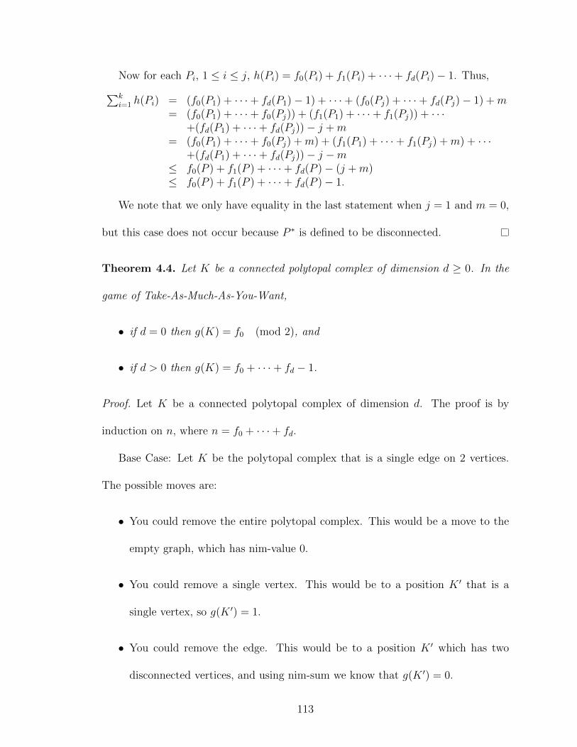
Now for each Pi, 1 ≤ i ≤ j, h(Pi) = f0(Pi) + f1(Pi) + · · ·+ fd(Pi)− 1. Thus,∑ki=1 h(Pi) = (f0(P1) + · · ·+ fd(P1)− 1) + · · ·+ (f0(Pj) + · · ·+ fd(Pj)− 1) +m
= (f0(P1) + · · ·+ f0(Pj)) + (f1(P1) + · · ·+ f1(Pj)) + · · ·+(fd(P1) + · · ·+ fd(Pj))− j +m
= (f0(P1) + · · ·+ f0(Pj) +m) + (f1(P1) + · · ·+ f1(Pj) +m) + · · ·+(fd(P1) + · · ·+ fd(Pj))− j −m
≤ f0(P ) + f1(P ) + · · ·+ fd(P )− (j +m)≤ f0(P ) + f1(P ) + · · ·+ fd(P )− 1.
We note that we only have equality in the last statement when j = 1 and m = 0,
but this case does not occur because P ∗ is defined to be disconnected.
Theorem 4.4. Let K be a connected polytopal complex of dimension d ≥ 0. In the
game of Take-As-Much-As-You-Want,
• if d = 0 then g(K) = f0 (mod 2), and
• if d > 0 then g(K) = f0 + · · ·+ fd − 1.
Proof. Let K be a connected polytopal complex of dimension d. The proof is by
induction on n, where n = f0 + · · ·+ fd.
Base Case: Let K be the polytopal complex that is a single edge on 2 vertices.
The possible moves are:
• You could remove the entire polytopal complex. This would be a move to the
empty graph, which has nim-value 0.
• You could remove a single vertex. This would be to a position K ′ that is a
single vertex, so g(K ′) = 1.
• You could remove the edge. This would be to a position K ′ which has two
disconnected vertices, and using nim-sum we know that g(K ′) = 0.
113
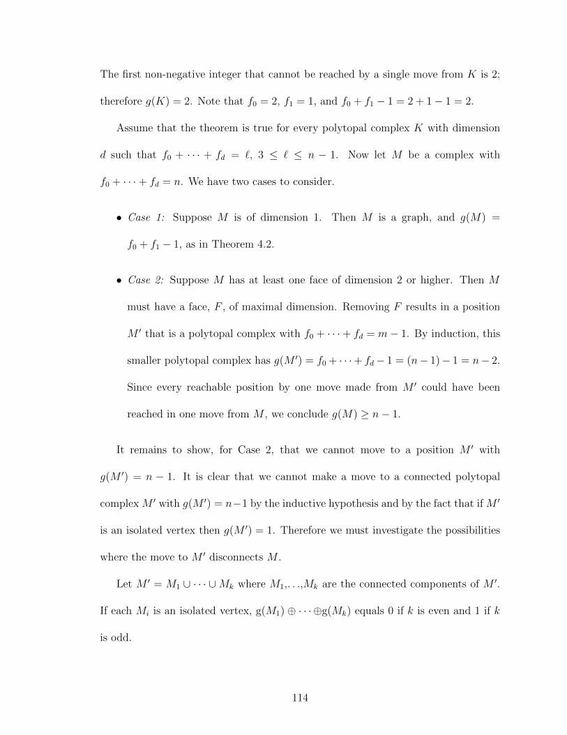
The first non-negative integer that cannot be reached by a single move from K is 2;
therefore g(K) = 2. Note that f0 = 2, f1 = 1, and f0 + f1 − 1 = 2 + 1− 1 = 2.
Assume that the theorem is true for every polytopal complex K with dimension
d such that f0 + · · · + fd = `, 3 ≤ ` ≤ n − 1. Now let M be a complex with
f0 + · · ·+ fd = n. We have two cases to consider.
• Case 1: Suppose M is of dimension 1. Then M is a graph, and g(M) =
f0 + f1 − 1, as in Theorem 4.2.
• Case 2: Suppose M has at least one face of dimension 2 or higher. Then M
must have a face, F , of maximal dimension. Removing F results in a position
M ′ that is a polytopal complex with f0 + · · ·+ fd = m− 1. By induction, this
smaller polytopal complex has g(M ′) = f0 + · · ·+ fd− 1 = (n− 1)− 1 = n− 2.
Since every reachable position by one move made from M ′ could have been
reached in one move from M , we conclude g(M) ≥ n− 1.
It remains to show, for Case 2, that we cannot move to a position M ′ with
g(M ′) = n − 1. It is clear that we cannot make a move to a connected polytopal
complex M ′ with g(M ′) = n−1 by the inductive hypothesis and by the fact that if M ′
is an isolated vertex then g(M ′) = 1. Therefore we must investigate the possibilities
where the move to M ′ disconnects M .
Let M ′ = M1 ∪ · · · ∪Mk where M1,. . .,Mk are the connected components of M ′.
If each Mi is an isolated vertex, g(M1) ⊕ · · ·⊕g(Mk) equals 0 if k is even and 1 if k
is odd.
114

Suppose not all Mi are isolated vertices. By Lemma 4.3, g(M1) ⊕ · · ·⊕g(Mk) ≤∑ki=1g(Mi) =
∑ki=1 h(Mi) < f0 + · · ·+ fn − 1.
Thus, we conclude that it is impossible to move from M to a position with nim-
value f0 + · · ·+ fd− 1, and since we can move to positions with nim-values 0 through
f0 + · · ·+ fd − 2, g(M) = f0 + · · ·+ fd − 1.
As with the graph version of Take-As-Much-As-You-Want, playing the game on a
single connected component is very uninteresting as player A will win every time by
taking the entire polytopal complex. This result does, however, provide the necessary
insight into the strategy for playing the game on multiple connected components,
which is a much more interesting game.
Copyright c© Kristen M. Barnard, 2017.
115

Chapter 5 Poset Games
The last stop on our journey through Take-Away on discrete structures brings us to
posets. The basic definitions that we need for this Chapter were given in Chapter 1.
The idea of Take-Away on a poset is not a new concept. In fact, several of the
well-known impartial games can be viewed as versions of Take-Away on a poset. If
the poset, P , is a finite totally ordered set—the Hasse diagram of P would just be a
chain—then the game of Take-Away is actually just the standard game of one-heap
Nim. Taking the product of two finite total orders of lengths k and `, respectively,
produces a poset isomorphic to the divisor lattice of an integer n = akb` where a and
b are prime. Removing the bottom element of this poset and playing Take-Away is
equivalent to the game Chomp (see Chapter 1). In a sense, Take-Away on a poset
without a unique bottom element can be viewed as a generalization of Chomp.
All of our previously examined Take-Away games can be viewed as poset Take-
Away games.
• A hypergraph, H, from Chapter 2 can be viewed as a poset, P , where the
vertices of H are the rank 0 elements of P and the hyperedges of H are the
rank 1 elements of P . A rank 1 element, u, covers a rank 0 element, v, if v is
a vertex of hyperedge u in the hypergraph. The rule for Type 1 Take-Away on
these posets is that when it is her turn a player may take at most one element
out of any single rank of P and if a rank 0 element is removed then any rank 1
116

elements covering it will also be removed.
• A hypergraph, H, can also be viewed as a poset, P , where the vertices of H are
the rank 0 elements of P and the hyperedges are ordered by set inclusion. In
this case, P might not be a ranked poset. The rule for Type 2 Take-Away on
these posets is that when it is her turn a player may take any element of the
poset, and in doing so she will also remove any element that is above it in the
poset.
• A polygonal complex, Q, from Chapter 3 can be viewed as a poset, P , where
the vertices of Q are the rank 0 elements of P , the edges of Q are the rank 1
elements of P , and the polygons in Q are the rank 2 elements of P . A rank 1
element, e, covers a rank 0 element, v, if v is a vertex of edge u in the polygonal
complex, and a rank 2 element p covers a rank 1 element e if e is an edge of
the polygon p. The rule for Type 2 Take-Away on these posets is that when it
is her turn a player may take at most one element out of any single rank of P ,
and she will take with it any element above it in the associated poset.
• A graph, G, from the Take-As-Much-As-You-Want game in Chapter 4 can be
viewed as a poset, P , where the vertices of G are the rank 0 elements of P and
the edges of G are the rank 1 elements of P . A rank 1 element, u, covers a rank
0 element, v, if v is a vertex of edge u in the graph. The rule for Take-As-Much-
As-You-Want on the poset is when it is her turn a player may take as many
elements as she desires from either rank of the poset, and any rank 0 element
117

that is removed takes with it any rank 1 elements covering it. There is a natural
extension of this to Take-As-Much-As-You-Want on polytopal complexes.
In this chapter we will look at results about Take-Away on a very specific type
of poset which we will call a rank-complete poset. We will first look at the standard
play of Take-Away on such a structure and fully describe the nim-values of positions
in the game. From there, we look at the game from a slightly different perspective,
namely that of misere play. Under misere play, the player that makes the last move
in the game is now the player that loses the game. We will fully describe nim-values
for rank-complete posets under misere play, and wrap up the chapter with further
results about misere play and rank-complete posets, namely finding nim-values for
the sum of rank-complete posets under misere Take-Away.
5.1 Take-Away on a Rank-Complete Poset
A rank-complete poset is a finite graded poset where every element in each rank n is
related to every element of rank n − 1. An example is shown in Figure 5.1. When
playing Take-Away on a rank-complete poset, a player may take any single element of
her choice out of any single rank of the poset, including rank 0. When an element is
removed, any elements of the poset related to it in a higher rank will also be removed.
Thus if a player takes an element with rank k, all elements of rank j ≥ k + 1 are
removed as well. Some examples of positions that can be reached in one move from
the poset in Figure 5.1 are in Figure 5.2.
The nim-values of rank-complete posets are very easily described based on the
118
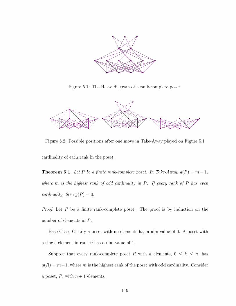
Figure 5.1: The Hasse diagram of a rank-complete poset.
Figure 5.2: Possible positions after one move in Take-Away played on Figure 5.1
cardinality of each rank in the poset.
Theorem 5.1. Let P be a finite rank-complete poset. In Take-Away, g(P ) = m+ 1,
where m is the highest rank of odd cardinality in P . If every rank of P has even
cardinality, then g(P ) = 0.
Proof. Let P be a finite rank-complete poset. The proof is by induction on the
number of elements in P .
Base Case: Clearly a poset with no elements has a nim-value of 0. A poset with
a single element in rank 0 has a nim-value of 1.
Suppose that every rank-complete poset R with k elements, 0 ≤ k ≤ n, has
g(R) = m+1, where m is the highest rank of the poset with odd cardinality. Consider
a poset, P , with n+ 1 elements.
119

• If every rank of P has even cardinality, any move made will be to a subposet of
P , P ′, where the highest rank has odd cardinality and the ranks below remain
unchanged and have even cardinality. Since P ′ has fewer elements, we have by
induction that g(P ′) = m′ + 1 where m′ is the lone rank of odd cardinality.
Hence we cannot move from P to a P ′ with nim-value 0, so we conclude that
g(P ) = 0.
• Assume P has at least one rank with odd cardinality. Let m be the highest
rank with odd cardinality in P . This means any rank above m in P will have
even cardinality. A move in the game made in one of these ranks to a position
P ′ will change the rank from even cardinality to odd cardinality, and since P ′
will have fewer elements than P , by induction g(P ′) > m+ 1.
We can also move to positions P ′ which have nim-values 0 through m. Suppose
you want to move to a P ′ with g(P ′) = j, 1 ≤ j ≤ m. This can be done in one
of two ways:
– If rank j−1 has even cardinality, make a move in this rank. The resulting
position will have rank j− 1 as the highest rank with odd cardinality, and
by induction g(P ′) = j.
– If rank j − 1 has odd cardinality in P , make a move in the next rank of
odd cardinality above rank j−1. Doing so will make rank j−1 the highest
rank with odd cardinality in P ′, and by induction g(P ′) = j.
Finally, to move to a position P ′ with g(P ′) = 0, make a move in the lowest
120

rank with odd cardinality. This will produce a position where each rank has
even cardinality, and by induction g(P ′) = 0.
We are, however, unable to move to a P ′ with g(P ′) = m+ 1. Since rank m of
P is of odd cardinality, making a move in this rank will change the cardinality
to even, and therefore the resulting position will have a nim-value less than
m + 1. Finally, any move made in a lower odd cardinality rank than m will
have g(P ′) < m+ 1. Therefore g(P ) = m+ 1.
We could view this game in a way closer to the standard version of one-heap Nim.
Instead of visualizing a Hasse diagram for playing this version of Take-Away, consider
having a heap of tokens of different colors, with all the tokens of the same color being
adjacent in the heap. For example, we could have some number of purple tokens with
a set of blue tokens stacked on top of them and finally a set of green tokens on top.
When it is her turn, a player could remove the top green token, the top blue token
along with all of the green tokens, or the top purple token along with all of the blue
and green tokens. As usual in Nim, the winner would be the player to remove the
final token from the heap.
Under either visualization—posets or heaps of tokens—one could easily evaluate
nim-values of the sum of these games. What is interesting about the sum of games
here, particularly when viewed in the token/heap sense, is that the structures which
have the same nim-value do not necessarily have to look similar at all. Since the
nim-value of the poset is determined by the highest rank of odd cardinality, all that
121

Figure 5.3: The Hasse diagram of a rank-complete poset with an extra element, t,appended beneath the rank 0 elements.
matters is that rank has an odd number of elements and any rank above it has an
even number of elements. The actual number of elements in that rank could be just
1 or perhaps 101, yet the two posets would have the same nim-value.
5.2 Misere Take-Away on a Rank-Complete Poset
Now, consider playing the same game, but instead of the winner being the player
to remove the last element from the poset we will say that the winner is the player
that forces her opponent to remove the last element from the poset. As previously
mentioned, this version of game play is referred to as misere play.
In this section we will fully describe the nim-values of rank-complete posets under
misere play. Much like misere play on one-heap Nim, the nim-values of many positions
do not change, and the positions that do change are the ones that have normal nim-
values of 0 or 1 [5]. For posets, we can study misere play in the same way we study
normal play by appending an extra element, t (referred to in most poset literature
as 0), covered by the rank 0 elements of P—we can then, in a sense, regard t as an
122

element with rank −1. An example is shown in Figure 5.3. We then have the added
condition that t cannot be removed until all other elements of the poset have been
removed; think of t as a buried treasure beneath the poset which we cannot claim
until it has been completely exposed via removing all elements of P . Let Pt = P ∪{t}.
Misere play on P is equivalent to normal play on Pt under the specified condition for
t. We will denote the misere nim-value of a poset P as gm(P ). Then gm(P ) =g(Pt).
Theorem 5.2. Let P be a rank-complete poset. When playing misere Take-Away on
P ,
• if the only rank with odd cardinality is rank 0, then gm(P ) = 0
• if every rank of the poset has even cardinality, then gm(P ) = 1, and
• otherwise gm(P ) =g(P ) = r + 1 where r is the highest rank of the poset that
has odd cardinality.
Proof. The proof is by induction on the number of elements in the poset.
Base Cases: Under misere play, ∅, the empty poset, is a losing position for the first
player; hence this position has gm(∅) =g(∅t) = 1. Let P be the poset that consists
of only one element. Then the first player can remove the element, leaving an empty
poset, which as we already discovered has nim-value 1; hence gm(P ) =g(Pt) = 0.
Let P be the poset which consists of two elements of rank 0 and no other elements.
Our only move is to the poset with just one element, which has nim-value 0; hence
gm(P ) =g(Pt) = 1. Lastly, let P be the poset with one element in rank 0 and one
element in rank 1 which covers the rank 0 element. Our only moves are to the empty
123

poset (with nim-value 1) or to the poset with only one element (with nim-value 0);
hence gm(P ) =g(Pt) = 2.
Suppose that in misere Take-Away the theorem is true for every rank-complete
poset P with k elements, 0 ≤ k ≤ n, n ≥ 2. Consider a poset, P , with n+ 1 elements
and let Pt be P with t located below the rank 0 elements.
• If the only rank with odd cardinality in P is rank 0, any move made on Pt in
rank j above rank 0 will be to a position P ′t with a rank of odd cardinality
above rank 0; by induction, gm(P ′) =g(P ′t) = j + 1 > 1. A move made on Pt
in rank 0 will be to a position P ′t with an even number of elements in rank 0
and no other elements in the poset; by induction, gm(P ′) =g(P ′t) = 1. Since no
other moves can be made, we conclude gm(P ) =g(P ′t) = 0.
• If every rank of P has even cardinality, any move made on Pt in rank j above
rank 0 will be to a position P ′t with rank j of odd cardinality; by induction,
gm(P ′) =g(P ′t) = j + 1 > 1. A move made on Pt in rank 0 will be to a position
P ′t with an odd number of elements in rank 0 and no other elements in the
poset; by induction, gm(P ′) =g(P ′t) = 0. Since no other moves can be made,
we conclude that the gm(P ) =g(Pt) = 1.
• Assume Pt has at least one rank above rank 0 with odd cardinality. Let r be
the highest rank with odd cardinality in P . This means any rank above r in
Pt will have even cardinality. A move in the game made in one of these ranks
will change that rank from even cardinality to odd cardinality, and since that
124

position will have fewer elements than Pt, by induction that position will have
a nim-value larger than r + 1. Thus gm(P ) =g(Pt) > r + 1.
We can also move to positions P ′t which have nim-values 2 through r. Suppose
you want to move to a P ′t with nim-value j, 2 ≤ j ≤ r. This can be done in
one of two ways:
– If rank j−1 has even cardinality, make a move in this rank. The resulting
position P ′ will have rank j − 1 as the highest rank with odd cardinality;
by induction gm(P ′) =g(P ′t) = j.
– If rank j−1 has odd cardinality in Pt, make a move in the next rank above
rank j − 1 which has odd cardinality. Doing so will make rank j − 1 the
highest rank with odd cardinality in P ′t , and by induction gm(P ′) =g(P ′t) =
j.
To move to a position P ′t with gm(P ′) =g(P ′t) = 0, we do one of two options:
– If rank 0 has even cardinality, make a move in this rank. The resulting
position P ′ will have rank 0 as the highest rank with odd cardinality; by
induction gm(P ′) =g(P ′t) = 0.
– If rank 0 has odd cardinality in Pt, make a move in the next rank above
rank 0 that has odd cardinality. Doing so will make rank 0 the highest
rank with odd cardinality in P ′t , and by induction gm(P ′) =g(P ′t) = 0.
Finally, to move to a position P ′t with gm(P ′) =g(P ′t) = 1, make a move in the
lowest rank with odd cardinality. This will produce a position where each rank
125

has even cardinality, and by induction gm(P ′) =g(P ′t) = 1.
We are, however, unable to move to a P ′ with gm(P ′) =g(P ′t) = r+ 1. Suppose
that in P (and hence in Pt) there is a rank s, 0 < s < r, with odd cardinality.
Removing an element of rank s results in a position P ′t with an even cardinality
at rank s and a fewer number of elements than Pt; hence, by induction, g(P ′t) ≤
s < r+1. Since rank r of P is of odd cardinality, making a move in this rank will
change the cardinality to even, and therefore the resulting position will have a
nim-value less than r+ 1. Since any rank that may exist in P above rank r has
even cardinality, making a move in any of these ranks will produce a position
with nim-value greater than r + 1. Therefore the gm(P ) =g(P ′t) = r + 1.
While either the standard version of Take-Away on a rank-complete poset or the
misere version are somewhat more interesting than regular one-heap Nim, at least
to the casual player, we see from the nim-values that the optimal play on a rank-
complete poset will make the game quite uninteresting, particularly in the misere
case. Since the positions with nim-value 0 are very specific—all ranks having even
cardinality for regular play and only rank 0 having odd cardinality for misere play—
the actual game play would be very tedious or very quick, but not very interesting.
In fact, with these facts about the game discovered there is no real value in knowing
the actual nim-values for all positions, just knowing where the zeros are is sufficient
for playing perfectly.
126

A way to make the game more complex—and hence more interesting—is to play
on the direct sum of posets. The direct sum of posets P and Q, also known as the
disjoint union of P and Q, is the poset P +Q whose elements are from the set P ∪Q
and that has its relation defined as for x, y ∈ P + Q, x ≤ y in P + Q if either x,
y ∈ P with x ≤ y in P or x, y ∈ Q with x ≤ y in Q [9]. For normal game play—play
such that the last player to move is the winner—we know that the nim-value of a
sum of game positions is the nim-sum of the nim-values of the individual positions.
(See Theorem 1.4). In the next section we will focus on the misere play of this sum.
5.3 Misere Take-Away on the Sum of Rank-Complete Posets
As we have seen and previously discussed, summing games certainly makes the game
play more challenging. In this section we provide a result on misere play on a sum of
games. We will consider the play of Take-Away on the sum of rank-complete posets,
P = P1 + · · ·+Pn, to be as follows: when it is her turn to move, a player may take an
element from any rank of one single summand poset, Pi, taking with it all elements
above it in that poset. The player that removes the last remaining element(s) from
the collection of posets loses the game.
Returning to the game of Nim, we consider misere play where the game has
multiple heaps. Let G be a game of k-heap Nim with misere play. The (misere) nim-
value is determined as follows: if G contains no heaps of size n ≥ 2 then gm(G) = 0
if k is odd and gm(G) = 1 if k is even—we note that this is the reverse of what we
find under normal play conditions. Otherwise, that is if G contains at least one heap
of size 2 or larger, then gm(G) =g(G) [8].
127
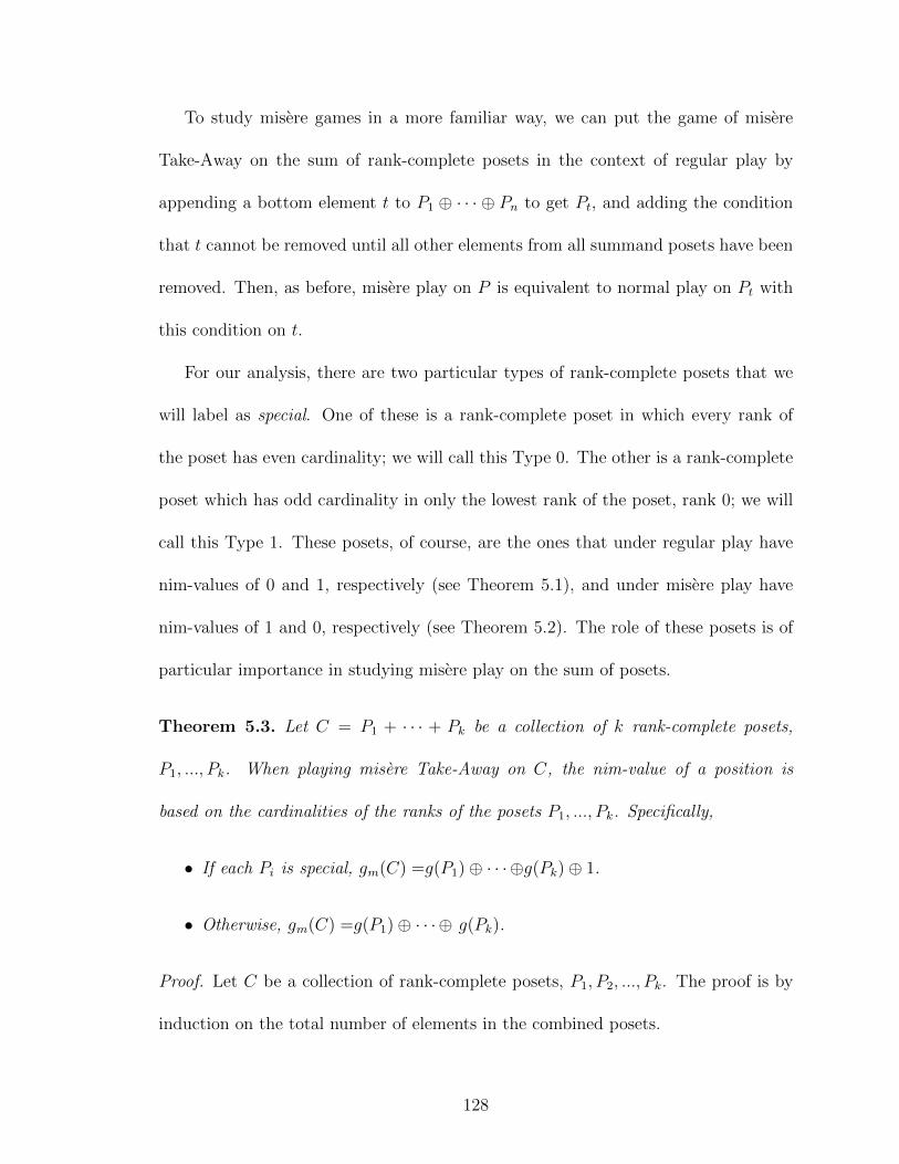
To study misere games in a more familiar way, we can put the game of misere
Take-Away on the sum of rank-complete posets in the context of regular play by
appending a bottom element t to P1 ⊕ · · · ⊕ Pn to get Pt, and adding the condition
that t cannot be removed until all other elements from all summand posets have been
removed. Then, as before, misere play on P is equivalent to normal play on Pt with
this condition on t.
For our analysis, there are two particular types of rank-complete posets that we
will label as special. One of these is a rank-complete poset in which every rank of
the poset has even cardinality; we will call this Type 0. The other is a rank-complete
poset which has odd cardinality in only the lowest rank of the poset, rank 0; we will
call this Type 1. These posets, of course, are the ones that under regular play have
nim-values of 0 and 1, respectively (see Theorem 5.1), and under misere play have
nim-values of 1 and 0, respectively (see Theorem 5.2). The role of these posets is of
particular importance in studying misere play on the sum of posets.
Theorem 5.3. Let C = P1 + · · · + Pk be a collection of k rank-complete posets,
P1, ..., Pk. When playing misere Take-Away on C, the nim-value of a position is
based on the cardinalities of the ranks of the posets P1, ..., Pk. Specifically,
• If each Pi is special, gm(C) =g(P1)⊕ · · ·⊕g(Pk)⊕ 1.
• Otherwise, gm(C) =g(P1)⊕ · · ·⊕ g(Pk).
Proof. Let C be a collection of rank-complete posets, P1, P2, ..., Pk. The proof is by
induction on the total number of elements in the combined posets.
128

Base Cases: Under misere play, ∅, the empty poset, is a losing position for the first
player; hence this position has gm(∅) =g(∅t) = 1. Let P be the poset that consists
of only one element. Then the first player can remove the element, leaving an empty
poset, which as we already discovered has nim-value 1; hence gm(P ) =g(Pt) = 0. Let
P be the poset which consists of two posets, P1 and P2, each with one element of
rank 0 and no other elements. Our only move is to the poset with just one element,
which has nim-value 0; hence gm(P ) =g(Pt) = 1. Lastly, let P be the poset with one
element in rank 0 and one element in rank 1 which covers the rank 0 element. Our
only moves are to the empty poset (with nim-value 1) or to the poset with only one
element (with nim-value 0); hence gm(P ) =g(Pt) = 2.
Without loss of generality, we can arrange the Pi in C so that all of the special
posets are together and all of the non-special posets are together. For convenience
we will rename the special posets Q1 through Qj, and rename the non-special posets
R1 through R`.
• If the position is made up of only special posets, there are two cases:
– Case 1: A move made in rank 0 of any poset in C will result in a C ′
which still has all special posets but has a fewer total number of elements.
Let s be the number of Type 1 special posets in C ′. If s is odd then
gm(C ′) = (0 ⊕ · · · ⊕ 0 ⊕ 1 ⊕ · · · ⊕ 1) ⊕ 1 = 0. For s to be odd then C
must have an even number of Type 1 special posets because either a Type
1 from C became a Type 0 in C ′ or a Type 0 from C became a Type 1 in
C ′. Likewise, if s is even then g(C ′) = (0⊕ · · · ⊕ 0⊕ 1⊕ · · · ⊕ 1)⊕ 1 = 1.
129
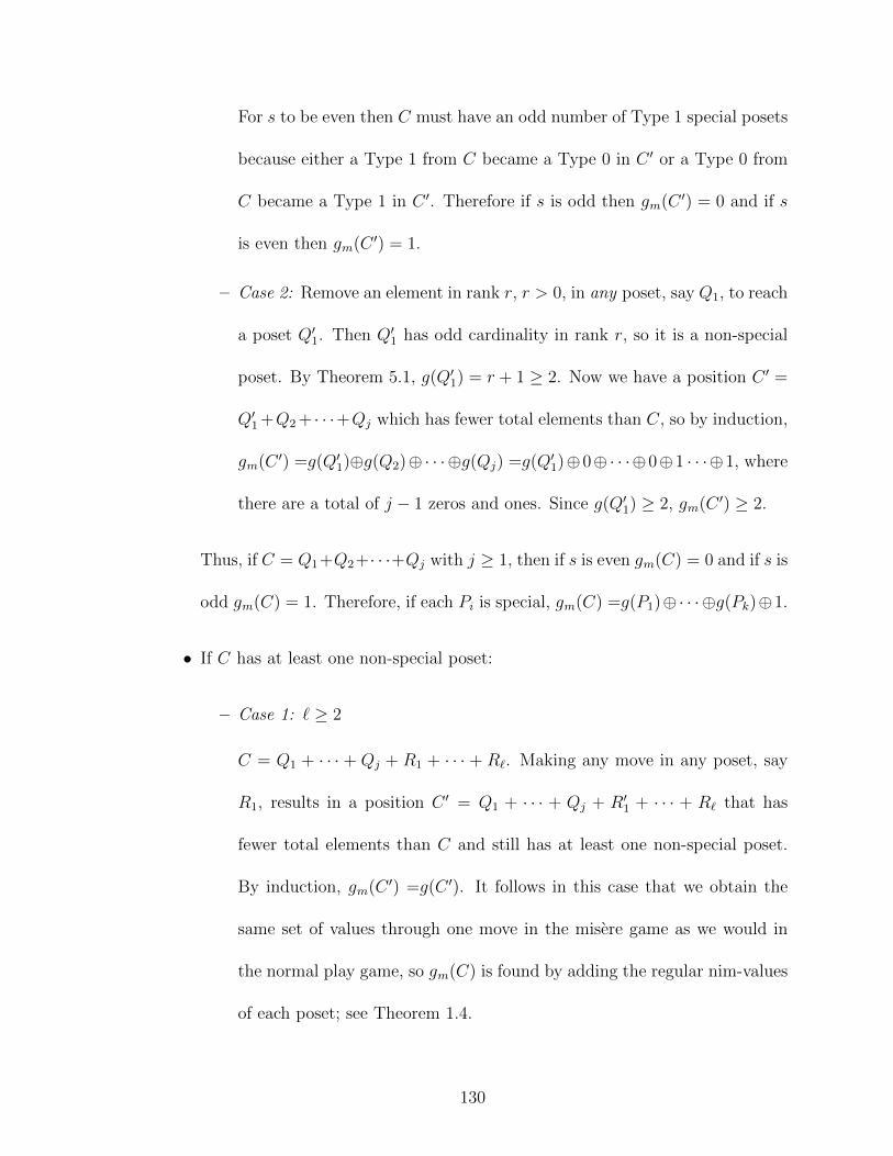
For s to be even then C must have an odd number of Type 1 special posets
because either a Type 1 from C became a Type 0 in C ′ or a Type 0 from
C became a Type 1 in C ′. Therefore if s is odd then gm(C ′) = 0 and if s
is even then gm(C ′) = 1.
– Case 2: Remove an element in rank r, r > 0, in any poset, say Q1, to reach
a poset Q′1. Then Q′1 has odd cardinality in rank r, so it is a non-special
poset. By Theorem 5.1, g(Q′1) = r + 1 ≥ 2. Now we have a position C ′ =
Q′1 +Q2 + · · ·+Qj which has fewer total elements than C, so by induction,
gm(C ′) =g(Q′1)⊕g(Q2)⊕· · ·⊕g(Qj) =g(Q′1)⊕0⊕· · ·⊕0⊕1 · · ·⊕1, where
there are a total of j − 1 zeros and ones. Since g(Q′1) ≥ 2, gm(C ′) ≥ 2.
Thus, if C = Q1+Q2+· · ·+Qj with j ≥ 1, then if s is even gm(C) = 0 and if s is
odd gm(C) = 1. Therefore, if each Pi is special, gm(C) =g(P1)⊕· · ·⊕g(Pk)⊕1.
• If C has at least one non-special poset:
– Case 1: ` ≥ 2
C = Q1 + · · · + Qj + R1 + · · · + R`. Making any move in any poset, say
R1, results in a position C ′ = Q1 + · · · + Qj + R′1 + · · · + R` that has
fewer total elements than C and still has at least one non-special poset.
By induction, gm(C ′) =g(C ′). It follows in this case that we obtain the
same set of values through one move in the misere game as we would in
the normal play game, so gm(C) is found by adding the regular nim-values
of each poset; see Theorem 1.4.
130

– Case 2: ` = 1
∗ Case 2a: Remove a rank 0 element from R1 to reach a poset R′1 that
is a special poset. Then C ′ = Q1 + · · · + Qj + R′1. By induction,
gm(C ′) = 0 or 1, depending on the value of j and whether R′1 is Type
0 special or Type 1 special.
∗ Case 2b: Remove an element from the lowest rank of odd cardinality
above rank 0 in R1 to reach a poset that is a special poset. Then
C ′ = Q1 + · · · + Qj + R′1. By induction, gm(C ′) = 0 or 1, depending
on the value of j and whether R′1 is Type 0 special or Type 1 special.
Further, the R′1 from Case 2a and the R′1 in this case are different
types of special posets, therefore one will have nim-value 0 and the
other have nim-value 1. Thus it is always possible to make move in
R1 that will yield a position with gm(C ′) = 0 and make a move in R1
that will yield a position with gm(C ′) = 1.
∗ Case 2c: Making any other move in R1 or any move any poset other
than R1, say Q1, results in a position C ′ that has fewer total elements
than C and still has at least one non-special poset. By induction,
gm(C ′) =g(C ′).
It follows in this case that we obtain the same set of values through one
move in the misere game as we would in the normal play game, so gm(C)
is found by adding the regular nim-values of each poset; see Theorem 1.4.
Thus, if C has at least one non-special poset, gm(C) =g(P1)⊕ · · ·⊕ g(Pk).
131
This result is a nice parallel of the relationship between g(P ) and gm(P ) for a
single rank-complete poset. In the earlier sections of this chapter we saw that the
nim-values under regular play and misere play were the same for most rank-complete
posets; the only places where the values actually differed were these special posets.
This result is also nice in that it generalizes misere play on multiple nim heaps. If
we were to consider a rank-complete poset with only one single element in each rank
this would be isomorphic to a nim heap. Playing Take-Away on a sum of these very
specific types of rank-complete posets, then, would be the same as playing a game of
multi-heap Nim, under both normal play conditions as well as misere play conditions.
With this game generalizing misere Nim, one might assume that the strategy for
misere play could be, as Conway describes, “play as in normal play until the game is
nearly over, and then make a sensible move” [5], alluding to the fact that misere Nim
is played as normal until the heaps are of size 1 and the game is nearly done. However,
Grundy showed that in general misere games can be much more complicated than
this strategy can allow [5].
Copyright c© Kristen M. Barnard, 2017.
132

Chapter 6 Areas for Further Research
Reflecting on all of the results presented in Chapters 2 through 5, we can see that there
are many opportunities for further research. The following questions are particularly
interesting.
• In Chapter 2 we saw from the analysis of the nim-values of the truncated tetra-
hedron that the nim-values are all between 0 and 7, but we have not identified
three unique characteristics about the hypergraph that could predict the nim-
value in the way that the parity of the number of edges and the parity of the
number of vertices did for the oddly uniform hypergraphs and the evenly uni-
form hypergraphs with a marked coloring. Will these hypergraphs with both
odd and even sized hyperedges with a marked coloring always have nim-values
between 0 and 7? Are there particular characteristics that can be identified
that will quickly predict the nim-values?
• In Chapter 3 there are several places for further study. As the size of the even
polygon increases and more tails are appended to the vertices, what patterns
can we observe in the nim-values? We saw that for an even polygon with 3 tails
the nim-values were very interesting and there seemed to be quite a few patterns
all working together, making it difficult to describe them succinctly. We did
notice, though, that in the places where the tail lengths seemed significantly far
apart and sufficiently large that the nim-values were often 4 or 7. Can we prove
133

that this will always be the case? Do interesting patterns arise when we append
more than one tail from a single vertex? What, if anything, is the connection
with the pattern found for the nim-values of an even polygon with one tail and
the pattern for the graph with a single odd cycle with a particular tree attached
to one vertex observed by Riehemann?
• In Chapter 4 we looked at the game of Take-As-Much-As-You-Want. What
would this game look like on a general hypergraph?
• In Chapter 5 we looked at Take-Away on a very specific type of poset, followed
by looking at misere play on one or more of these posets. From here, questions
arise about studying Take-Away on other types of posets and looking for pat-
terns in their nim-values. Also, the investigation into misere play suggests that
it might be interesting to take a look at misere play on the other games in this
dissertation.
• How would the nim-values change if the rules of any of these games were altered
to include limited options for a player to pass, that is not make a move, when
it is her turn? Of course we cannot allow a pass at every turn, since this could
prevent the game from terminating.
• It happens that in many combinatorial games that at some positions of the
game with nonzero nim-value that there are multiple positions within one move
of the game that have nim-value 0. Is one of these winning positions a better
choice than the others in terms of efficiency, e.g., guaranteeing to end the game
134

sooner? For small games this could be checked using a directed graph with all
the possible positions of the game as the vertices and investigating recursively
from the final winning positions. This task will quickly get out of hand as the
size of the game increases. Is there another way to study these games with
efficiency as a factor in the winning strategy?
Copyright c© Kristen M. Barnard, 2017.
135

Bibliography
[1] Michael H. Albert, Richard J. Nowakowski, and David Wolfe. Lessons in play.A K Peters, Ltd., Wellesley, MA, 2007.
[2] Kristof Berczi, Attila Bernath, and Mate Vizer. A note on V−free 2−matchings.manuscript, retrieved from “arXiv” 1505.03717v1, 2015.
[3] Elwyn R. Berlekamp, John H. Conway, and Richard K. Guy. Winning ways foryour mathematical plays. Volume 1. A K Peters, Ltd., Wellesley, MA, 2001.
[4] J. A. Bondy and U.S.R. Murty. Graph theory with applications. Elsevier SciencePublishing Co., Inc, New York, fifth edition, 1982.
[5] John H. Conway. On numbers and games. Academic Press, New York, 1976.
[6] Tirasan Khandhawit and Lynnelle Ye. Chomp on graphs and subsets.manuscript, retrieved from “arXiv” 1101.2718v1, 2011.
[7] Robert M. Riehemann. Subset take-away on graphs, dissertation, University ofKentucky, Lexington, KY, 2003.
[8] Aaron N. Seigel. Combinatorial game theory, volume 146 of Graduate Studies inMathematics. Amer. Math. Soc., Providence, RI, 2013.
[9] Richard P. Stanley. Enumerative combinatorics. Volume 1, volume 49 of Cam-bridge Studies in Advanced Mathematics. Cambridge University Press, Cam-bridge, second edition, 2012.
[10] Douglas B. West. Introduction to graph theory, Prentice-Hall, Inc, Upper SaddleRiver, NJ, second edition, 2001.
[11] Gunter M. Ziegler. Lectures on polytopes, volume 152 of Graduate Texts inMathematics. Springer-Verlag, New York, 1995.
136

Vita
Kristen Michelle Barnard
Place of Birth
• London, Kentucky
Educational Experience
• Eastern Kentucky University, Richmond, KYM.S. in Mathematics, May 2006
• Eastern Kentucky University, Richmond, KY
– B.S., Mathematics, May 2004
– A.S., Science for Engineering, May 2004
summa cum laude, Honors Scholar
Professional Positions
• Mathematics Instructor, Berea College, Berea, KY 2007-present
• Adjunct Instructor, Berea College, Berea, KY 2006-2007
• Adjunct Instructor, Eastern Kentucky University, Richmond, KY 2006-2007
• Graduate Fellow, Project ISMAM, Eastern Kentucky University, Richmond,KY 2004-2006
• Undergraduate Fellow, Project ISMAM, Eastern Kentucky University, Rich-mond, KY 2003-2004
• MathExcel Teaching Assistant, Eastern Kentucky University, Richmond, KY2002-2004
Service
• Teacher Education Committee, Berea College, Berea, KY 2014-2017
• Pi Mu Epsilon Faculty Mentor, Berea College, Berea College, Berea, KY 2014-present
• Kappa Mu Epsilon Secretary, Eastern Kentucky University, Richmond, KY2003-2004
• Kappa Mu Epsilon Treasurer, Eastern Kentucky University, Richmond, KY2002-2003
137