some tools for model adaptation in the context of fluid flows
TRANSCRIPT

Some tools for model adaptation in the context offluid flows
Edwige Godlewski
February 25-27, 20149th DFG - CNRS WORKSHOP
Micro-Macro Modeling and Simulation of Liquid-Vapor Flows
Edwige Godlewski Some tools for model adaptation in the context of fluid flows

collaborations
Frederic Coquel (CMAP, Ecole Polytechnique)Clement CancesHelene Mathis (LMJL, U. Nantes)Nicolas Seguin
LRC MANON
Edwige Godlewski Some tools for model adaptation in the context of fluid flows

Introduction
Model adaptation, multiscale modeling• Duality based methods, linked to a goal oriented strategy:output functional J(u) (example drag computation, pressure pointvalue). Rannacher (2009); Oden, Prudhomme et al (2006);Braack, Ern (2003)u ∈ V , a(u)(φ) + d(u)(φ) = (f , φ), ∀φ ∈ Vum ∈ V , a(um)(φ) = (f , φ), ∀φ ∈ Vestimate the influence of neglecting d(u) on J(u).
• Heterogeneous Multiscale Method, W. E, Engquist et al.(2007)capture the macroscale behavior of a system with the help ofmicroscale models.• In between, multiscale kinetic-fluid solver: kinetic-fluid regionsand coupled model. Fluid model everywhere, localized kineticupscaling P. Degond, G. Dimarco, L. Mieussens 2010: micro-macrodecomposition f = E [%] + g (local equilibrium + deviation part).Localization of fluid-kinetic transition and dynamic coupling.
Edwige Godlewski Some tools for model adaptation in the context of fluid flows

Introduction
• Domain decomposition• and geometrical multiscale modeling Formaggia, Gerbeau,
Nobile, Quarteroni (2001) for flows in compliant vessels orMalleron, Zaoui, Goutal, Morel (2011) Efficient model coupling inhydroinformatics (dynamic coupling of existing 2D-1D codes).
• Shi Jin, Jian-guo Liu and Li Wang Math. Comp. (2013) Adomain decomposition method for semilinear hyperbolic systemswith two-scale relaxations; provides a rigourous analysis in thelinear case (solution by Laplace transform).
• We follow the strategy developed in Braack, Ern (2003): “achieve compromise between accuracy of the model andcomputational costs by increasing adaptivity.• next step: change locally the model or the mesh size; balancingmodel and mesh size.” by adding posteriori error control Kroner,Ohlberger 1999 and adaptivity M. Ohlberger (2009) (scalar case)
Edwige Godlewski Some tools for model adaptation in the context of fluid flows

Application
Context (LRC)
Edwige Godlewski Some tools for model adaptation in the context of fluid flows

Introduction
Simulation of multiphase flow in nuclear energy industry (CEA):coolant circuits are formed by different components, each one withits associated specific model for the coolant flow. The coolant is atwo-phase fluid.There exists a wide variety of models (mixture, drift, homogeneousor not, two-fluid, multi-field models...):- according to the main features of the flow (immiscible, dispersed,3D effects, ...)- according to what one is interested in (fluid velocity / acousticwaves,...)- more or less costly to implement (number of variables, complexpressure laws,...)- more or less accurate (thermal, mechanical, dynamical equilibria).→ Build a (numerical) strategy to choose the “right” one at the“right” place: adaptative procedure.Begin by some academic case: 2 models, linked by some hierarchy.
Edwige Godlewski Some tools for model adaptation in the context of fluid flows

Outline
Model adaptation
Framework
Relaxation / equilibrium models
Adaptation procedure in the relaxation framework
A toy model (theoretical validation)
Edwige Godlewski Some tools for model adaptation in the context of fluid flows

Our framework for model adaptation
In the context of two-phase flows: many (numerical) models.We assume there exists a fine / accurate / expensive model valideverywhere and also a coarse / less accurate / cheaper model.Goal: build a (numerical) strategy to choose the right one, definethe regions where one uses each model.
fine / coarse models Mfi/Mco : a hierarchy between them
right means a balance between tolerance of less accuracy(measured by an indicator) and cost
nonlinear approach, non stationary
domain decomposition: fine / coarse (space) domains Dfi/Dco
dynamic adaptation define D(n)fi/co at each time step tn
Need to couple Mfi/Mco at a sharp* interface Dnfi ∩ Dn
co
(fixed on [tn, tn+1])
* regularized for the toy model
Edwige Godlewski Some tools for model adaptation in the context of fluid flows

Our framework for model adaptation
Hierarchy between the 2 systems given by relaxation (otherprocess: averaging, homogenization, linearization, viscousapproximation, low Mach regime, ...)Assumptions:
models given by a system of PDE’s (conservation laws,hyperbolicity required) linked by relaxation
Mfi Relaxation system / Mco Equilibrium systemEx: HRM/HEM (Homogeneous Relaxation/Equilibrium Model)
here analysis of 1D problems, for simplicity Dfi/Dco ⊂ Rfinite volume (conservative) schemes
balance cost / accuracy: use a coarse (less expensive) modelwhenever acceptable and fine model elsewhere: D = Dco ∪Dfi
use a (sharp) interface coupling model
Edwige Godlewski Some tools for model adaptation in the context of fluid flows

Theoretical frame: some tools
• Sharp interface coupling model, as general as possible (flux orstate coupling): G-Raviart, (2004), Ambroso et al. (2008)...• well understood (theoretical results) on significative examples• numerical interface coupling procedures for general situations• regularized (thickened) interface for regularity results Boutin etal. (2011)
• Hierarchy between systems is linked to a relaxation process:Mfi Relaxation system →Mco Equilibrium system as relaxationtime ε→ 0Again well understood on significative examples:
• fluid models (theoretical results) Coquel-G-Seguin (2012)• HRM / HEM (phase transition) Ambroso et al. (2007)• more complicated: bifluid / drift model; Baer-Nunziato /
two-component Euler system Dellacherie (2003)• Hierarchy may be inherited by numerical scheme• Possible to couple numerically with different schemes
Edwige Godlewski Some tools for model adaptation in the context of fluid flows

Some principles for model adaptation
• Some issues: which model (coarse/fine)? how do we switch?estimate of modeling error?Relaxation system considered as fine, more accurate, moreexpensive / equilibrium system as coarse, cheaper. Both are given.
• Need of:- an indicator (involving the relaxation time ε) which measures themodeling error- a tolerance θ for this error- a dynamic procedure: uad (., tn)→ uad (., tn+1)- a numerical indicator should NOT need compute the fine solutioneverywhere, only uad (., tn)• Validate the approach on• simpler models: for which hierarchy between models can beproved and with compatible numerical schemes• numerical extension to more general cases (different schemes)• a toy model: theoretical results can be obtained
Edwige Godlewski Some tools for model adaptation in the context of fluid flows
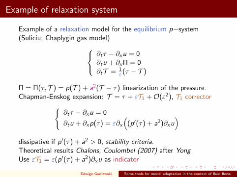
Example of relaxation system
Example of a relaxation model for the equilibrium p−system(Suliciu; Chaplygin gas model)
∂tτ − ∂xu = 0∂tu + ∂x Π = 0∂tT = 1
ε (τ − T )
Π = Π(τ, T ) = p(T ) + a2(T − τ) linearization of the pressure.Chapman-Enskog expansion: T = τ + εT1 +O(ε2), T1 corrector{
∂tτ − ∂xu = 0
∂tu + ∂xp(τ) = ε∂x
((p′(τ) + a2)∂xu
)dissipative if p′(τ) + a2 > 0, stability criteria.Theoretical results Chalons, Coulombel (2007) after YongUse εT1 = ε(p′(τ) + a2)∂xu as indicator
Edwige Godlewski Some tools for model adaptation in the context of fluid flows
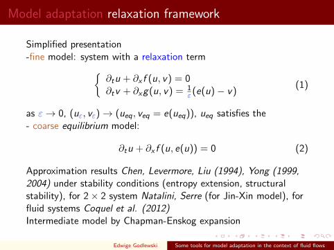
Model adaptation relaxation framework
Simplified presentation-fine model: system with a relaxation term{
∂tu + ∂x f (u, v) = 0∂tv + ∂xg(u, v) = 1
ε (e(u)− v)(1)
as ε→ 0, (uε, vε)→ (ueq, veq = e(ueq)), ueq satisfies the- coarse equilibrium model:
∂tu + ∂x f (u, e(u)) = 0 (2)
Approximation results Chen, Levermore, Liu (1994), Yong (1999,2004) under stability conditions (entropy extension, structuralstability), for 2× 2 system Natalini, Serre (for Jin-Xin model), forfluid systems Coquel et al. (2012)Intermediate model by Chapman-Enskog expansion
Edwige Godlewski Some tools for model adaptation in the context of fluid flows
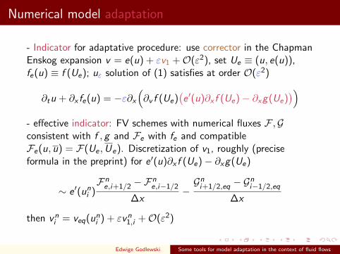
Numerical model adaptation
- Indicator for adaptative procedure: use corrector in the ChapmanEnskog expansion v = e(u) + εv1 +O(ε2), set Ue ≡ (u, e(u)),fe(u) ≡ f (Ue); uε solution of (1) satisfies at order O(ε2)
∂tu + ∂x fe(u) = −ε∂x
(∂v f (Ue)
(e ′(u)∂x f (Ue)− ∂xg(Ue)
))- effective indicator: FV schemes with numerical fluxes F ,Gconsistent with f , g and Fe with fe and compatibleFe(u, u) = F(Ue ,Ue). Discretization of v1, roughly (preciseformula in the preprint) for e ′(u)∂x f (Ue)− ∂xg(Ue)
∼ e ′(uni )Fn
e,i+1/2 −Fne,i−1/2
∆x−Gn
i+1/2,eq − Gni−1/2,eq
∆x
then vni = veq(un
i ) + εvn1,i +O(ε2)
Edwige Godlewski Some tools for model adaptation in the context of fluid flows

Numerical model adaptation
Given: two models, fine Mfi and coarse Mco , associated FVschemes with numerical fluxes gfi , gco ; an indicator δn(x) of the‘model error’; a tolerance θ.The principle is: at each time step, compute the coarse modelMco
whenever possible: if solution too far ( δ > tolθ) from equilibrium,use the fine model and at interface one couples the two models.Numerical model adaptation scheme: compute a piecewiseconstant solution noted uad (., tn) following the algorithm:on one time step tn → tn+1, starting from uad (., tn)
compute δn+1 everywhere
determine Dnfi : if δn(x) ≥ θ, x ∈ Dn
fi
solve Mfi with gfi in Dnfi : gives (u, v)(x , tn+1), x ∈ Dn
fi
solve Mco with gco in Dnco = D \ Dn
fi , gives u(x , tn+1),x ∈ Dn
co , v = e(u)
couple them at interface Dnfi ∩ D
nco :
Edwige Godlewski Some tools for model adaptation in the context of fluid flows

coupling Numerical interface coupling
Finite Volume method: interface at j = 0, cells Cj+1/2 = (xj , xj+1)
un+1j+1/2 = un
j+1/2 −∆t
∆x(gnα,j+1 − gn
α,j ), j ∈ Z
with α = L for j ≤ −1,R, j ≥ 0, we have 2 conservative FVschemes, in x < 0 and in x > 0.Non conservative approach: TWO fluxes at the interface x = 0
gnL,0 = gL
(un−1/2,u
n+1/2
), gn
R,0 = gR
(un−1/2,u
n+1/2
)
x=0
,0g R ,0g
x 1 x 1x 2 x 21/2u
t
xu1/2
L
Edwige Godlewski Some tools for model adaptation in the context of fluid flows

Adaptation results
• Theoretical relaxation framework with entropy extension (EE).scheme for relaxation system: splitting convection / source(implicit)scheme for equilibrium (coarse) system: deduced withinstantaneous relaxation (fine scheme has AP property).Numerical illustration on a test case satisfying the EE condition.• Numerical illustration on test cases which do not satisfy the EE:
• 2D experiment with a phase transition HRM/HEM model(extended entropy is not strictly convex)
• 1D experiment with Baer Nunziato (7 equations) - bicomponent(4 equations); different (non compatible) schemes: Rusanov forconvection + successive splitting of the relaxation terms; withChapman-Enskog type indicatorcf. Helene Mathis et al. preprint 2013
Edwige Godlewski Some tools for model adaptation in the context of fluid flows

Adaptation a toy scalar example
In order to prove some results (theoretical validation, no CPUgain!) we consider• fine model: 2× 2 system (relaxation){
∂tu + ∂x f (u, v) = 0,∂tv = 1
ε (veq(x)− v),(3)
g = 0, e(u) = veq(x), so that we can compute explicitly the ODEfor v (decoupled)• coarse scalar conservation law (equilibrum, ε→ 0)
∂tu + ∂x f (u, veq(x)) = 0
Theoretical results are possible: obtained by comparing ufi and uad
respective solution of equation with fluxFfi (u, x , t) = f (u, vfi (x , t)) ad Fad (u, x , t) = f (u, vad (x , t)), wherevad obtained by the adaptation algorithm.
Edwige Godlewski Some tools for model adaptation in the context of fluid flows

Adaptation a toy scalar example
Use results for comparing solution u, v of CL with resp. fluxes f , g ,resp. i. d. u0, v0: need smooth fluxes → a smooth vad → thickenthe interface.Algorithm: steps tn → tn+1, n ≥ 0 with tk = k∆ta, starting from(u−1
ad , v−1ad ) = (u0, v0):
• Indicator: v(n)i exact solution of (3) with initial data v
(n−1)ad (., tn)
(recall that vco = veq)
• Dnfi = {x , |veq(x , t)− v
(n)i (x , t)| > ∆taΣ,
|∂xveq(x , t)− ∂xv(n)i (x , t)| > ∆taΣ′ or |∂xxv
(n)i (x , t)| > Σ′′}
• regularized caracteristic function χδ(x , t) = 1 on D(n)fi = 0 if
distance d(x ,D(n)f ) ≥ δ.
• Define v(n)ad = χv
(n)i + (1− χ)veq
• Define u(n)ad entropy solution on (tn, tn+1] of equation with flux
Fad = f (u, vad ) and data u(n−1)ad (., tn)
Edwige Godlewski Some tools for model adaptation in the context of fluid flows
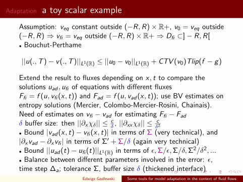
Adaptation a toy scalar example
Assumption: veq constant outside (−R,R)× R+, v0 = veq outside(−R,R) ⇒ vfi = veq outside (−R,R)× R+ ⇒ Dfi ⊂]− R,R[• Bouchut-Perthame
||u(.,T )− v(.,T )||L1(R) ≤ ||u0 − v0||L1(R) + CTV (v0)Tlip(f − g)
Extend the result to fluxes depending on x , t to compare thesolutions uad , ufi of equations with different fluxesFfi = f (u, vfi (x , t)) and Fad = f (u, vad (x , t)); use BV estimates onentropy solutions (Mercier, Colombo-Mercier-Rosini, Chainais).Need of estimates on vfi − vad for estimating Ffi − Fad
δ buffer size: then ||∂xχδ|| ≤ cδ , ||∂xxχδ|| ≤ c
δ2
• Bound |vad (x , t)− vfi (x , t)| in terms of Σ (very technical), and|∂xvad − ∂xvfi | in terms of Σ′ + Σ/δ (again very technical)• Bound ||uad (t)− ufi (t)||L1(R) in terms of ε,Σ/ε,Σ/δ,Σ2/δ2, ...• Balance between different parameters involved in the error: ε,time step ∆a; tolerance Σ, buffer size δ (thickened interface)
Edwige Godlewski Some tools for model adaptation in the context of fluid flows

Theorem||uad − ufi ||C([0,T ];L1(R)) ≤ cΣ1/2
Numerical illustrationcf. preprint C. Cances et al. (2013)
Edwige Godlewski Some tools for model adaptation in the context of fluid flows

Conclusion and future work
• Model adaptation• an original approach involving coupling of existing codes• indicator well founded in the relaxation framework(Chapman-Enskog)• some convincing numerical illustrations validate the approach• theoretical result on a toy problem
• A lot remains to do!• include numerical error estimate (Chainais, Kroner-Ohlberger)• extend the formalism to some other criteria (indicator) on modelexamples; other ε, small parameter (other hierarchy: Machnumber, fluctuation,... )• other models (hyperbolic-parabolic, convection dominatedviscous flow)• link with other approaches (goal oriented)• ...
Thank you for your attentionEdwige Godlewski Some tools for model adaptation in the context of fluid flows