SONG IDENTIFICATION USING THE NUMENTA PLATFORM

FOR INTELLIGENT COMPUTING

A Bachelors of Science Honors Thesis

Presented in Partial Fulfillment of the Requirements for

Graduation with Distinction from the

Department of Computer Science and Engineering at

The Ohio State University

By:

Nathan C. Schey

*****

The Ohio State University

May 2008

Bachelor‟s Examination Committee: Approved By:

Dr. Rajiv Ramnath, Advisor

Dr. Mikhail Belkin Advisor

Department of Computer

Science and Engineering

ii

ABSTRACT

Hierarchical Temporal Memory (HTM) technology is a new computing paradigm based

on the structure and function of the human neocortex [15]. HTM networks are the cornerstone

technology in the Numenta Platform for Intelligent Computing (NuPIC), a new tool for artificial

intelligence research developed by Numenta Incorporated. NuPIC provides researchers with a

series of tools that they can use to train and test their HTM networks. Ultimately the developers

of NuPIC believe that the long term applications will include image analysis, robotics, data

mining, and intelligent systems for traffic monitoring and weather prediction [7]. However, up to

this point HTM networks have only been used to develop a simple vision system that is limited to

recognizing a small set of line drawings. Before researchers can claim to have realized the

ultimate promise of NuPIC, they must utilize the technology to solve problems across wide range

of subjects. The purpose of the research presented in this thesis is to provide an experience report

of HTM technology and identify best practices for future HTM researchers. In order to facilitate

this experience a solution to the non-trivial problem of song identification was developed. This

problem is well-researched and hundreds of papers have been written that range from using signal

processing techniques [13] to sampling an artist‟s work for unique features [16]. Several

advanced solutions using existing technologies have been created and developing an equivalent

solution to this problem using NuPIC helped identify several areas in need of more in-depth

research.

iii

In order to ensure that a successful song identification development experience was

reached, several preparatory steps were taken. At the beginning of this research NuPIC was a

relatively new artificial intelligence framework and there were no established processes for

design, implementation, or testing. To remedy this shortcoming, NuPIC‟s extensive training

material was used to develop a more formal methodology for using the technology. One of the

first steps in this newly created process was to develop an in-depth understanding of the data

being used. In order gain this knowledge multiple digital music formats were researched. This

analysis revealed that the Midi music format was the best candidate to produce data for HTM

network consumption. The next step was then to use the Midi song data to run several song

identification experiments using NuPIC in order to test different encoding schemes and diverse

HTM network structures. A data encoding scheme based on melodic segmentation yielded an

identification accuracy of 100% and supports the conclusion that NuPIC is a valid platform for

further research in the area of song identification. The song identification development

experience also identified several areas in need of more in-depth research. Many of the

algorithms used in HTM networks are designed to work with very specific data encoding

schemes. In order for HTM technology to gain more widespread use, these algorithms must be

improved. HTM networks also require that input data follows a strict partition-based format.

Switching to a XML-based data input format would allow researchers to quickly generate and

validate data sets. Lastly, the development experience presented in this thesis shares many

similarities with the development processes created by the data mining community. Researchers

wishing to increase their likelihood of success should look for ways to incorporate the data

mining community‟s knowledge into their research.

iv

ACKNOWLEDGMENTS

I would like to thank my advisor Dr. Rajiv Ramnath for the freedom he granted me in

pursuing a research topic that interested me. His support and flexibility was crucial as I

attempted to balance my research with several cooperative education rotations. I would also like

to thank my family for their support and encouragement throughout my college career. Five

years ago I could never have envisioned the opportunities available to me and I owe my success

to the strong work ethic they instilled in me over the years.

v

TABLE OF CONTENTS

Abstract ...................................................................................................................................... ii

Acknowledgments ..................................................................................................................... iv

List of Figures........................................................................................................................... vii List of Tables ............................................................................................................................ vii

Chapters:

1. Introduction .................................................................................................................. 10

2. Problem Formulation .................................................................................................... 12

3. Related Work .............................................................................................................. 14

3.1. Hierarchical Temporal Memory ............................................................................. 14

3.1.1. HTM Network Behavior ......................................................................... 14

3.1.2. Node Algorithms .................................................................................... 18 3.2. Song Identification ................................................................................................ 22

4. Song Identification Development Experience................................................................ 23

4.1. Research Process ................................................................................................... 23

4.2. Exploration of Representation Schemes ................................................................. 29

4.2.1. Sample Based Audio Files ...................................................................... 30 4.2.2. Midi Audio Files .................................................................................... 37

4.2.3. Local Boundary Detection Model ........................................................... 38

4.3. Software Tools Used .............................................................................................. 39 4.3.1. HTM Tools ............................................................................................ 39

4.3.2. Data Preparation Tools ........................................................................... 40

4.4. Piano Roll HTM Network ...................................................................................... 41

4.4.1. Data Representation Scheme .................................................................. 41 4.4.2. HTM Network Design ............................................................................ 43

4.4.3. Evaluating HTM Network Results .......................................................... 44

4.5. Melodic Segmentation HTM Network ................................................................... 46 4.5.1. Data Representation Scheme .................................................................. 46

4.5.2. HTM Network Design ............................................................................ 48

vi

4.5.3. Evaluating HTM Network Results .......................................................... 50

5. Discussion .................................................................................................................... 51

5.1. Analysis of HTM Node Algorithms ....................................................................... 51

5.2. Development Process ............................................................................................. 53 5.3. Data Set Format ..................................................................................................... 56

5.4. Future Work .......................................................................................................... 56

Bibliography ............................................................................................................................. 58

vii

LIST OF FIGURES

Figure 3.1: A sample HTM network. ......................................................................................... 17

Figure 3.2: HTM Node Structure [5]. ........................................................................................ 18

Figure 3.3: Spatial Pooler quantization example. ....................................................................... 19

Figure 3.4: Time adjacency matrix operation [5]. ...................................................................... 19

Figure 3.5: Temporal Pooler group formation [5]. ..................................................................... 21

Figure 4.1: The NuPIC development process. ............................................................................ 24

Figure 4.2: Sample training data file. ......................................................................................... 25

Figure 4.3: Sample HTM network creation script. ..................................................................... 27

Figure 4.4: Sample HTM network training script. ...................................................................... 28

Figure 4.5: HTM network analysis using the Vitamin D Toolkit. ............................................... 29

Figure 4.6: Audio waveform using 10 second sample period. .................................................... 31

Figure 4.7: Audio waveform using 1 second sample period. ...................................................... 31

Figure 4.8: Sample Fourier Transform plots. ............................................................................. 33

Figure 4.9: Fourier Transform taken over 10 millisecond song clip. ........................................... 35

Figure 4.10: Mels Scale versus Hertz Scale plot. ....................................................................... 36

Figure 4.11: LBDM melodic analysis [3].................................................................................. 39

Figure 4.12: Midi Toolbox piano roll graph. .............................................................................. 41

Figure 4.13: Piano roll HTM network layout. ............................................................................ 44

viii

Figure 4.14: Graph of the local boundary detection algorithm. ................................................... 47

Figure 4.15: Window based data generation algorithm. ............................................................. 48

Figure 4.16: Melodic segmentation HTM network structure. ..................................................... 49

Figure 5.1: Position error in the spatial pooler. .......................................................................... 51

Figure 5.2: Difficultly of recognizing patterns in noisy data [1]. ................................................ 53

Figure 5.3: Sample iterative data mining process developed by Berry and Linoff. ...................... 55

ix

LIST OF TABLES

Table 4.1: Sample Midi note matrix data structure. .................................................................... 37

Table 4.2: Piano roll 2-D array structure. ................................................................................... 42

Table 4.3: Piano roll confusion matrix. ..................................................................................... 45

Table 4.4: Five song melodic segmentation HTM confusion matrix. .......................................... 50

10

CHAPTER 1

INTRODUCTION

The Numenta Platform for Intelligent Computing (NuPIC) [1] is an emerging artificial

intelligence framework which is based on the biological structure of the human brain. The

creators of NuPIC believed that in order to simulate human intelligence using computers, one

must first understand how the human brain worked. Their initial research culminated in an

overarching theory for neuroscience that stated that human intelligence was centered in the

neocortex and that a single, powerful algorithm is implemented by every region of the human

neocortex [6]. This biological theory was then used to derive a computational theory for

intelligence based upon the structure of the human brain called Hierarchical Temporal Memory

(HTM). HTM networks replicate the structure and function of the human cortex, but are not

limited by the same biological input constraints as humans. Since the cortical algorithm in the

human brain is universal, almost any data stream can be input into a HTM network and expert

systems can be developed across a wide range of topics [7]. For example, an intelligent traffic

system could be developed by exposing the HTM network to data from traffic sensors, speed

monitoring sensors, and traffic lights. This is possible because HTMs work by receiving arbitrary

11

data streams and proceed to uncover the underlying temporal and spatial patterns in the data.

These patterns are then compared those stored in memory and beliefs regarding the causes of

sensory data are propagated throughout the hierarchy [7].

12

CHAPTER 2

PROBLEM FORMULATION

While HTMs are a new type of memory designed for modern computers, they cannot be

programmed using traditional techniques such as writing C++ code. To enable researchers to

build applications using HTMs, Numenta Incorporated released the Numenta Platform for

Intelligent Computing (NuPIC). NuPIC is an extensible platform that implements a runtime

engine designed for HTM network simulation and provides researchers with a series of tools that

they can use to train and test their HTMs [1]. NuPIC is designed to solve problems that involve

identifying patterns in large data sets. The range of applications NuPIC will be used to solve

likely include image analysis, robotics, data mining, and intelligent systems such as traffic

monitoring and weather prediction [7].

When one looks at the goals of NuPIC, it is difficult not to be skeptical. The developers

of NuPIC have only used it to solve a simple problem that involves identifying several line

drawings [14]. Before the promises of NuPIC can be realized, it must be used to solve several

problems of significance. The purpose of the research presented in this thesis is to provide a

NuPIC experience report by using it to develop a solution to the non-trivial problem of song

identification. Before this research could take place, several topics had to be researched in order

to gain the required base of knowledge for running song identification experiments using NuPIC.

The first topic dealt with overcoming NuPIC‟s lack of best practices for HTM network

13

development. In order to remedy this shortcoming, a development process had to be created that

would allow researchers to iteratively train and test their HTM networks. However, the process

could only succeed when coupled with an in-depth understanding of digital music formats. An

investigation of digital music formats allowed several different encoding algorithms to be

developed, which were then used to generate input data for HTM network experiments. After the

preparatory steps were complete, song identification experiments using NuPIC could be carried

out. The results of these experiments were then analyzed and they revealed several areas of

NuPIC in need of more in-depth research.

14

CHAPTER 3

RELATED WORK

3.1. Hierarchical Temporal Memory

3.1.1. HTM Network Behavior

The structure of a HTM network is intended to mirror the nested hierarchical structure of

real world objects [6]. This structure includes both spatial and temporal components. In order to

illustrate this, imagine that one is attempting to build a HTM network to regulate and monitor

freeway traffic. One approach might be to install sensors along the highway that can track cars

passing by key junctions and road sensors to monitor distances between individual cars. A

fundamental concept of HTMs is that the input data must contain both temporal and spatial

components and an examination of the traffic data complies with this rule [15]. The temporal

aspect of the traffic data is illustrated by the „ripple effect‟ that one driver can cause by braking,

inadvertently affecting traffic for miles. This phenomenon would be nearly impossible to detect

using data from a single point in time and could only be found by observing changes in the data

over time from a set of geographically diverse traffic sensors. The spatial component can be

found by examining data on a micro level and monitoring the distances between individual cars.

Unlike the „ripple effect‟, it would be possible to examine a data snapshot from a small number of

sensors and identify cars that were tailgating. This example also illustrates a fundamental trait of

15

HTM networks: Patterns emerge at multiple levels in the hierarchy [7]. A micro level effect like

tailgating could be quickly identified using data from a limited number of traffic sensors to

calculate the distance between two consecutive cars. A macro level pattern such as the „ripple

effect‟ would occur much higher in the hierarchy as traffic must be examined over a greater

distance and time frame.

HTM networks are designed as a hierarchy of nodes, where each node has 2 phases of

execution: training and inference [1]. Regardless of position within the hierarchy each node

executes the same algorithm, but they operate at different levels of abstraction. When being

trained, the network undergoes an iterative process where all nodes on a level are trained

concurrently. Once a level is finished being trained, it is switched to inference mode and training

is initiated on the next level. This pattern continues up the hierarchy until all nodes have been

trained. During the training phase, HTM nodes on the bottom level receive direct sensory data

and beliefs about the causes of the data propagate throughout the network [5]. Over time the

HTM network uses these beliefs to build a model of its environment by observing how the beliefs

behave over time [7]. Once a node is switched to inference mode the HTM refines its model by

attempting to group the patterns it has learned. The model is further refined upon each iteration,

until the top level category node is ready for training. The category node monitors the beliefs of

its children and uses a category input file to perform supervised learning. Once the top level node

is finished training, it is set to inference mode and the network is ready to be tested.

During inference novel data is presented to the bottom nodes and beliefs about the causes

of sensory input propagate throughout the hierarchy. Data flows both ways in the hierarchy and a

change in a high level node can affect the beliefs of a lower level node via a technique known as

belief propagation [6]. As time progresses beliefs are formed by all nodes, but more complex and

abstract beliefs occur higher in the hierarchy. These beliefs are then combined at the top level

16

category node and the HTM outputs a belief vector, where each element in the vector contains the

percentage likelihood that a specific type of input category is causing the current sensory data [1].

It is important to note that the structure of the HTM network does not have to be uniform and

nodes can be connected to multiple parents. Figure 3.1 shows a possible HTM network structure

and illustrates how beliefs about a single input vector propagate throughout the hierarchy.

17

Figure 3.1: A sample HTM network.

18

3.1.2. Node Algorithms

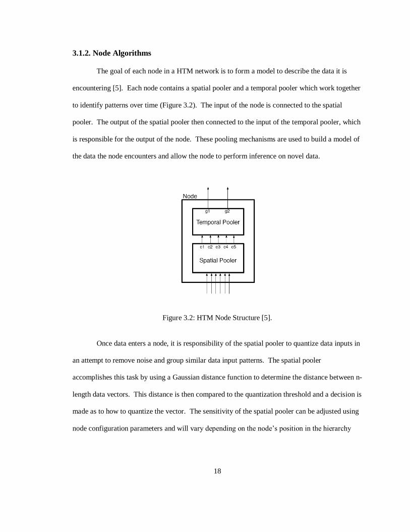
The goal of each node in a HTM network is to form a model to describe the data it is

encountering [5]. Each node contains a spatial pooler and a temporal pooler which work together

to identify patterns over time (Figure 3.2). The input of the node is connected to the spatial

pooler. The output of the spatial pooler then connected to the input of the temporal pooler, which

is responsible for the output of the node. These pooling mechanisms are used to build a model of

the data the node encounters and allow the node to perform inference on novel data.

Figure 3.2: HTM Node Structure [5].

Once data enters a node, it is responsibility of the spatial pooler to quantize data inputs in

an attempt to remove noise and group similar data input patterns. The spatial pooler

accomplishes this task by using a Gaussian distance function to determine the distance between n-

length data vectors. This distance is then compared to the quantization threshold and a decision is

made as to how to quantize the vector. The sensitivity of the spatial pooler can be adjusted using

node configuration parameters and will vary depending on the node‟s position in the hierarchy

19

[1]. Figure 3.3 shows several sample data vectors and displays how the spatial pooler would

quantize the data.

Distance between [1 1 1 1 1] and [1 1 0.99 1 1.02]

Quantization Threshold = 0.1, vectors are equal

Distance between [1 1 1 1 1] and [1 3 1.5 1 0.1]

Quantization Threshold = 0.1, vectors are different

Figure 3.3: Spatial Pooler quantization example.

The quantized data is then input into the temporal pooler, which attempts to pool together

patterns based on their temporal proximity [5]. When a node is in learning mode, it records

which patterns occur near each other in time and stores the data in a time adjacency matrix.

Figure 3.4 displays how the matrix is structured and stores temporal proximity information.

Figure 3.4: Time adjacency matrix operation [5].

20

After a node is switched to inference mode, it examines this matrix and attempts to group patterns

with high temporal proximity. The temporal pooler accomplishes this by converting the time

adjacency matrix into an undirected weighted graph [5]. Each quantization point represents a

vertex and edge weights between quantization points depend on their temporal proximity.

Temporal groups are identified by examining the graph for connected components and grouping

together components based on edge strength. These groups are used when attempting to form

beliefs about novel data and the output of a node is in terms of the temporal groups it has learned

[5]. The memory and time adjacency edge strength threshold of the temporal pooler is

configurable via node parameters and must be configured according to the data the node is

encountering. Figure 3.5 displays several iterations of the temporal group formation process.

21

Figure 3.5: Temporal Pooler group formation [5].

22

3.2. Song Identification

The majority of music identification and classification research is conducted through the

International Music information Retrieval Systems Evaluation Laboratory (IMIRSEL) Project.

The organization holds yearly competitions in categories such as song identification and genre

classification [9]. A large amount of the research is done using Midi music files, though some

researchers are working with more complex sample based audio formats. Researchers involved

with the IMIRSEL Project have had many years to refine traditional approaches and create hybrid

artificial intelligence algorithms. Their research is now at a highly advanced stage and

researchers are starting to combine multiple audio features to make their systems more robust [12,

16]. Unfortunately, due to the complexity of feature extraction and hybrid AI algorithms, this

work is not accessible to entry level researchers.

23

Chapter 4

SONG IDENTIFICATION DEVELOPMENT EXPERIENCE

4.1. Research Process

NuPIC is a relative newcomer to the AI world and has no established set of best

practices. The unique nature of HTM networks makes the traditional software development

process of requirements analysis, design, implementation, and testing irrelevant. A major hurdle

in this research was to come up with a scientific process that would allow for iterative

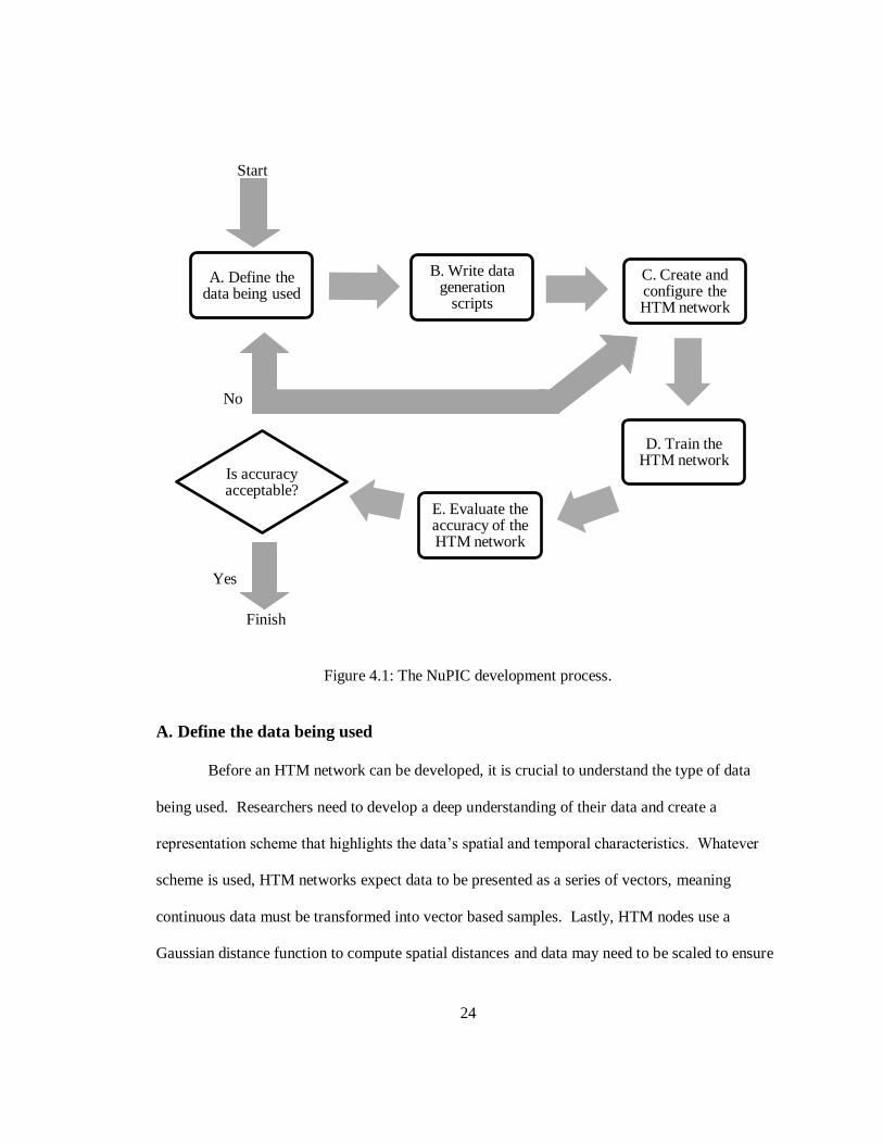
development and experimentation with different HTM network configurations. An iterative

process based on the NuPIC documentation was developed and revised throughout the research

project. The final NuPIC development process is presented in Figure 4.1.

24

Figure 4.1: The NuPIC development process.

A. Define the data being used

Before an HTM network can be developed, it is crucial to understand the type of data

being used. Researchers need to develop a deep understanding of their data and create a

representation scheme that highlights the data‟s spatial and temporal characteristics. Whatever

scheme is used, HTM networks expect data to be presented as a series of vectors, meaning

continuous data must be transformed into vector based samples. Lastly, HTM nodes use a

Gaussian distance function to compute spatial distances and data may need to be scaled to ensure

A. Define the data being used

B. Write data generation

scripts

C. Create and configure the HTM network

D. Train the HTM network

E. Evaluate the accuracy of the HTM network

Is accuracy acceptable?

Yes

Finish

No

Start

25

proper results [5]. There is rarely a simple answer to the multitude of questions presented in the

data transformation stage and this step will be revisited many times throughout the HTM

development process.

B. Write data generation scripts

Any programming language can be used to generate data sets for a HTM network. For a

typical network, each data set contains two files: 1) A data file of input vectors where each vector

is placed on a new line in the file 2) A category file where every row correctly categorizes the

corresponding vector in the data file [1]. In order to properly train and test a network two distinct

sets are used. Overall the format of the training and test data sets are very similar, but there is one

crucial difference. Training data sets allow the researcher to insert specially formatted data

vectors (a data vector of „0‟s) to reset the temporal memory of the HTM [1]. This becomes

important during supervised learning when the data vectors switch from one category to another

because it prevents the temporal pooler from looking for patterns that do not exist. The following

figure displays the format of a training data file:

Figure 4.2: Sample training data file.

0.7935 0.4761 0.0000 0.4761 0.0000 0.3053 0.3045 0.0000 0.0385 0.0362

0.0036 0.0000 0.4761 0.0000 0.1471 0.2013 0.3053 0.0000 0.7935 0.0000

0.0000 0.3526 0.0000 0.4761 0.0000 0.2013 0.0000 0.3053 0.0000 0.3322

0.0409 0.0000 0.7935 0.0000 0.4761 0.0000 0.4761 0.0000 0.3053 0.1768

0 0 0 0 0 0 0 0 0 0

0.0000 0.6448 0.5069 0.0000 0.5069 0.0000 0.1767 0.5069 0.0000 0.0000

0.2013 0.4240 0.5069 0.5675 0.5069 0.3543 0.0000 0.5069 0.5676 0.7567

26

C. Create and configure the HTM network

HTM networks are built and configured by writing Python scripts. While the

majority of the script follows a standard pattern, each network requires customization.

Researchers must leverage in-depth knowledge of their data to design and configure the

hierarchy of nodes. Each node‟s algorithms need to be customized based on the input

values it is encountering. Because of the large number of node parameters, node

configuration values will most likely be tweaked each iteration in order to improve

accuracy. Luckily the network structure will usually remain the same, reducing the

amount of code that must be change. Figure 4.3 displays a sample network creation

Python script.

#-------------------------------------------------------- # create the initial instance of the network

#--------------------------------------------------------

network = Network()

#--------------------------------------------------------

# Create data and category sensors

#--------------------------------------------------------

dataSensor = CreateNode("VectorFileSensor", phase=0, dataOut=80)

network.addElement("dataSensor", dataSensor)

category = CreateNode("VectorFileSensor", phase=2, dataOut=1)

network.addElement("categorySensor", category)

#--------------------------------------------------------

# Create and add Level 1 region, containing 4 nodes

#--------------------------------------------------------

level1 = Region(4,

CreateNode("Zeta1Node",phase=1,bottomUpOut=200,symmetricTime=False,

spatialPoolerAlgorithm="gaussian",maxDistance=0.001,

sigma=0.01,transitionMemory=4,topNeighbors=1,maxGroupSize=20,

temporalPoolerAlgorithm="sumProp",detectBlanks=1

)

)

network.addElement("level1", level1)

#--------------------------------------------------------

# Create and add Level 2 region, containing 2 nodes

#--------------------------------------------------------

level2 = Region(2,

CreateNode("Zeta1Node",phase=2,bottomUpOut=100,symmetricTime=False,

spatialPoolerAlgorithm="Gaussian”,maxDistance=0.001,

sigma=0.01,transitionMemory=4,topNeighbors=1,

maxGroupSize=10,temporalPoolerAlgorithm="sumProp",

detectBlanks=1

)

)

27

network.addElement("level2", level2)

#--------------------------------------------------------

# Create supervised node at the top level

#--------------------------------------------------------

topLevel = CreateNode("Zeta1TopNode", phase=3, categoriesOut=5,

spatialPoolerAlgorithm="product", mapperAlgorithm="sumProp")

network.addElement("topLevel", topLevel)

#--------------------------------------------------------

# Create file effector to write outputs of top level node to a text file

#--------------------------------------------------------

output = CreateNode("VectorFileEffector", phase=4)

network.addElement("fileOutput", output)

#--------------------------------------------------------

# Link the HTM network together

#--------------------------------------------------------

network.link("dataSensor", "level1", SimpleSensorLink())

network.link("level1", "level2", SimpleFanIn())

network.link("level2", "topLevel", SimpleFanIn())

network.link(source="categorySensor", sourceOutputName="dataOut",

destination="topLevel", destinationInputName="categoryIn")

network.link(source="topLevel", sourceOutputName="categoriesOut",

destination="fileOutput", destinationInputName="dataIn")

#--------------------------------------------------------

# save the network to disk

#--------------------------------------------------------

network.writeXML(“HTMNetwork.xml”)

Figure 4.3: Sample HTM network creation script.

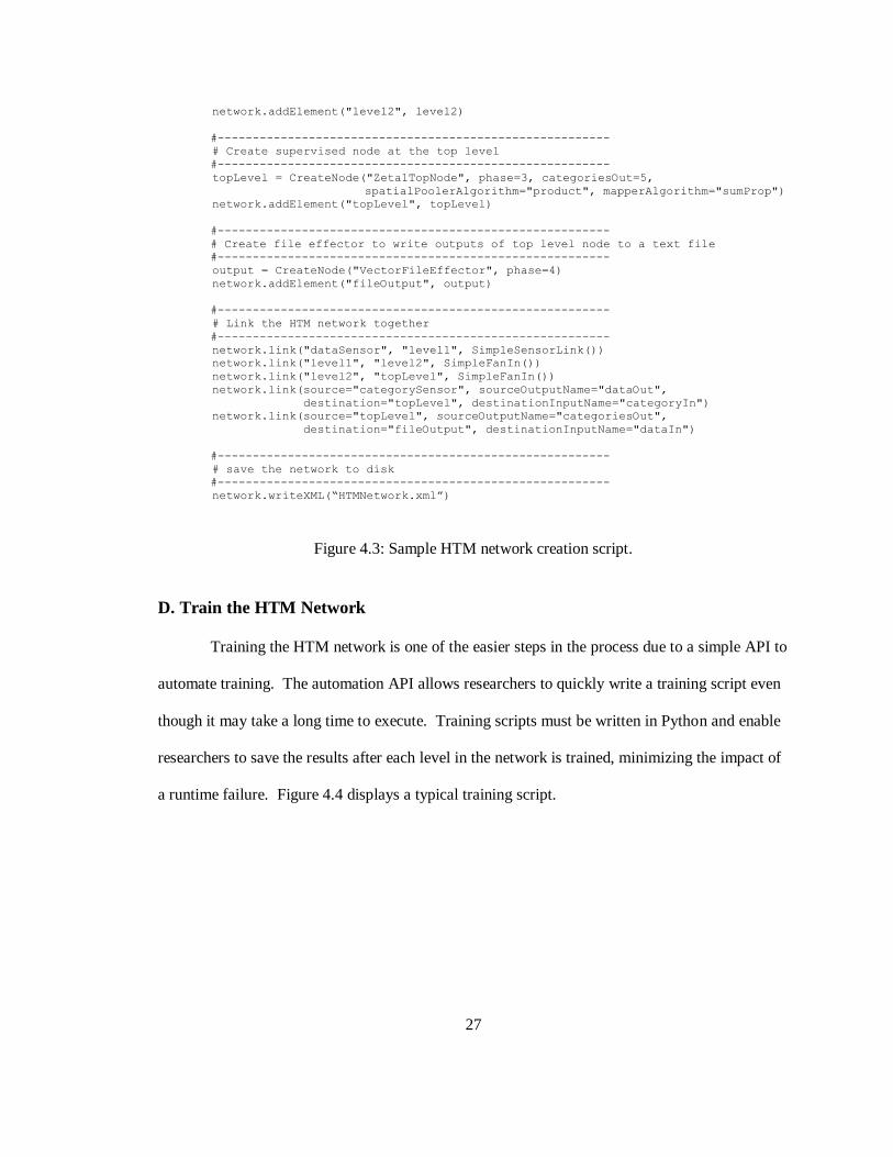
D. Train the HTM Network

Training the HTM network is one of the easier steps in the process due to a simple API to

automate training. The automation API allows researchers to quickly write a training script even

though it may take a long time to execute. Training scripts must be written in Python and enable

researchers to save the results after each level in the network is trained, minimizing the impact of

a runtime failure. Figure 4.4 displays a typical training script.

28

#--------------------------------------------------------

# Load network and prepare data files we will use.

#--------------------------------------------------------

runtimeNet = CreateRuntimeNetwork(untrainedNetworkFile, files=[trainDataFile,

trainCategoryFile])

dataSensor = runtimeNet.getElement("dataSensor")

categorySensor = runtimeNet.getElement("categorySensor")

dataSensor.execute("loadFile", trainDataFile)

categorySensor.execute("loadFile", trainCategoryFile)

rows = 5000

#--------------------------------------------------------

# Train Level 1

#--------------------------------------------------------

runtimeNet.run(Zeta1Train("level1", rows), ["dataSensor", "level1"])

runtimeNet.writeXML(“PostLevel1.xml”)

#--------------------------------------------------------

# Train Level 2

#--------------------------------------------------------

dataSensor.setParameter("position", "0")

categorySensor.setParameter("position", "0")

runtimeNet.run(Zeta1Train("level2", rows), ["dataSensor", "level1", "level2"])

runtimeNet.writeXML(“PostLevel2.xml”)

#--------------------------------------------------------

# Train Top Level Category Node

#--------------------------------------------------------

dataSensor.setParameter("position", "0")

categorySensor.setParameter("position", "0")

runtimeNet.run(Zeta1Train("topLevel", rows), exclusion=["fileOutput"])

#--------------------------------------------------------

# Save the network and retrieve trained network file from bundle

#--------------------------------------------------------

runtimeNet.writeXML(“TrainedNetwork.xml”)

runtimeNet.cleanupBundleWhenDone()

Figure 4.4: Sample HTM network training script.

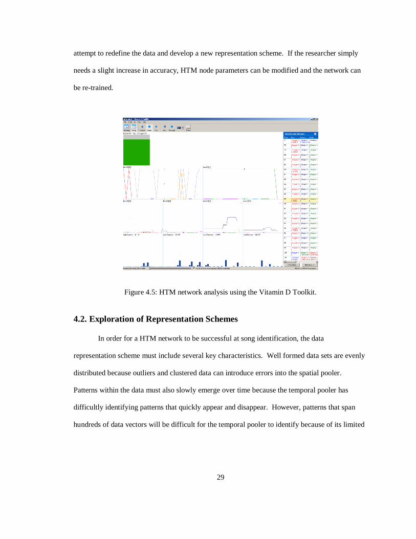
E. Evaluate the Accuracy of the HTM Network

Once the training script has finished executing, the Vitamin D Toolkit can be used to load

the network and interactively step through the test data set (Figure 4.5). The toolkit allows

developers to assess the network accuracy as a whole, as well as investigate how the beliefs of

individual nodes affect the network. This is especially helpful when trying to isolate the source

of incorrect inferences. If the results of the test are not satisfactory, the researcher has two

options. When the low accuracy is due to a poor data representation scheme, the researcher can

29

attempt to redefine the data and develop a new representation scheme. If the researcher simply

needs a slight increase in accuracy, HTM node parameters can be modified and the network can

be re-trained.

Figure 4.5: HTM network analysis using the Vitamin D Toolkit.

4.2. Exploration of Representation Schemes

In order for a HTM network to be successful at song identification, the data

representation scheme must include several key characteristics. Well formed data sets are evenly

distributed because outliers and clustered data can introduce errors into the spatial pooler.

Patterns within the data must also slowly emerge over time because the temporal pooler has

difficultly identifying patterns that quickly appear and disappear. However, patterns that span

hundreds of data vectors will be difficult for the temporal pooler to identify because of its limited

30

temporal memory. Lastly, each category that the HTM is trying to learn should have its own set

of unique patterns. This will allow the HTM to discover which patterns can be used to correctly

identify a category.

4.2.1. Sample Based Audio Files

Modern day digital music is stored electronically via an extremely complicated and

accurate data format. Researchers in the field must be educated in both audio theory and

computer science to fully comprehend music encoding methodologies. Popular formats such as

wav, mp3, ogg, or wma are all built on the same fundamental concept of sampling and differ only

in their strategy for compression. Of these formats, the wav format was chosen for deeper

analysis due to its relatively uncompressed and straightforward encoding format [18].

Compression makes it difficult to extract the wave samples from the music file and an

uncompressed format requires less preprocessing of the audio waveform. Figure 4.6 shows a

typical audio waveform using a 10 second sampling period and Figure 4.7 displays a subsection

of the same waveform over a 1 second sample period.

31

Figure 4.6: Audio waveform using 10 second sample period.

Figure 4.7: Audio waveform using 1 second sample period.

32

Standard wav files sample the audio waveform at a rate of 44,100 samples per second.

This creates a large, rapidly changing data set that is difficult to use when training HTM

networks. The large amount of variance makes it challenging for the spatial pooler to quantize

the data vectors, which in turn overwhelms the temporal pooler with a large amount of unique

data vectors. This results in a time adjacency graph with a large amount of low-weight edges.

The high connectedness of the graph makes it very difficult for the temporal pooler to identify

distinct groups within the graph. A popular data processing technique used to summarize a

waveform involves building a Discrete Fourier Transform over a predetermined segment of data.

This transform can be used to determine the power of the wave over the human audible frequency

spectrum [10]. Since the Fourier transform provides a plot of frequency versus power, it is often

possible to identify specific frequencies being played within the waveform. Therefore the Fourier

Transform data has the potential to identify chords and uncover melodic patterns by examining

consecutive segments. Figure 4.8 shows a Fourier Transform created using 1 second segments

from two different points in the song.

33

Figure 4.8: Sample Fourier Transform plots.

34

Even though the transforms shown in Figure 4.8 are taken from different sections of the

song, they are difficult to differentiate. Fourier Transforms created using 1 second segments are

too generic and the segment size needs to be reduced in order to isolate the notes being played by

each instrument. However, this approach is problematic due to the fact that the number of

samples in the segment affects the accuracy of the Fourier Transform. For example, using a

segment size of 44,100 samples (1 second) results in 22,050 data points to describe the frequency

spectrum. While this large amount of data points is sufficient to characterize the frequency

spectrum, it is too large a time frame to isolate the unique melodic elements of a song. A smaller

sample size such as 10 milliseconds would be better suited to isolate melodic elements, but results

in just 220 data points. This lack of data resolution becomes a problem when dealing with lower

pitch notes, where single octaves can span as little as 25Hz. Figure 4.9 shows a Fourier

Transform created using a segment size of 10 milliseconds. Upon close examination of Figure

4.9 it is possible to see linear interpolation between the data points, inaccurately summarizing

important data in the process. This figure illustrates the segment size and data resolution problem

with the Fourier Transform, making it a poor candidate to produce data for a HTM network.

35

Figure 4.9: Fourier Transform taken over 10 millisecond song clip.

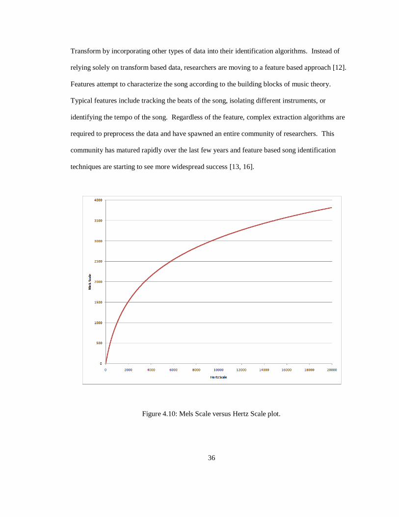
A technique often used to overcome the Fourier Transform data accuracy and time

tradeoff is to compute a set of Mel Frequency Cepstral Coefficients (MFCCs) for the segment.

These coefficients are calculated using the Mel Scale, which more closely resembles human

auditory recognition because it is based on a logarithmic scale (Figure 4.10) [11]. While the

MFCCs are promising, the initial step of this technique requires that a Fourier Transform be

computed on the segment. For a large segment size, the MFCCs effectively summarize the data

points created by the Fourier Transform. The problem comes when trying to identify melodic

components of the song. In order to do this effectively, one must decrease the segment size.

Hence this approach also confronts the data accuracy and time tradeoff issue associated with

Fourier Transforms. Other researchers are attempting to overcome the pitfalls of the Fourier

36

Transform by incorporating other types of data into their identification algorithms. Instead of

relying solely on transform based data, researchers are moving to a feature based approach [12].

Features attempt to characterize the song according to the building blocks of music theory.

Typical features include tracking the beats of the song, isolating different instruments, or

identifying the tempo of the song. Regardless of the feature, complex extraction algorithms are

required to preprocess the data and have spawned an entire community of researchers. This

community has matured rapidly over the last few years and feature based song identification

techniques are starting to see more widespread success [13, 16].

Figure 4.10: Mels Scale versus Hertz Scale plot.

37

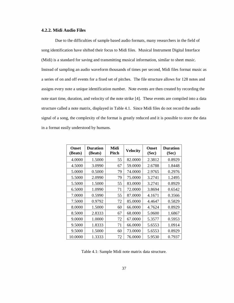
4.2.2. Midi Audio Files

Due to the difficulties of sample based audio formats, many researchers in the field of

song identification have shifted their focus to Midi files. Musical Instrument Digital Interface

(Midi) is a standard for saving and transmitting musical information, similar to sheet music.

Instead of sampling an audio waveform thousands of times per second, Midi files format music as

a series of on and off events for a fixed set of pitches. The file structure allows for 128 notes and

assigns every note a unique identification number. Note events are then created by recording the

note start time, duration, and velocity of the note strike [4]. These events are compiled into a data

structure called a note matrix, displayed in Table 4.1. Since Midi files do not record the audio

signal of a song, the complexity of the format is greatly reduced and it is possible to store the data

in a format easily understood by humans.

Onset

(Beats)

Duration

(Beats)

Midi

Pitch Velocity

Onset

(Sec)

Duration

(Sec)

4.0000 1.5000 55 82.0000 2.3812 0.8929

4.5000 3.0990 67 59.0000 2.6788 1.8448

5.0000 0.5000 79 74.0000 2.9765 0.2976

5.5000 2.0990 79 75.0000 3.2741 1.2495

5.5000 1.5000 55 83.0000 3.2741 0.8929

6.5000 1.0990 71 72.0000 3.8694 0.6542

7.0000 0.5990 55 87.0000 4.1671 0.3566

7.5000 0.9792 72 85.0000 4.4647 0.5829

8.0000 1.5000 60 66.0000 4.7624 0.8929

8.5000 2.8333 67 68.0000 5.0600 1.6867

9.0000 1.0000 72 67.0000 5.3577 0.5953

9.5000 1.8333 71 66.0000 5.6553 1.0914

9.5000 1.5000 60 73.0000 5.6553 0.8929

10.0000 1.3333 72 76.0000 5.9530 0.7937

Table 4.1: Sample Midi note matrix data structure.

38

4.2.3. Local Boundary Detection Model

Regardless of the music file format chosen, the goal is to encode the music for playback

at a future date. These goals create more work for the HTM network because it must discover

melodic and chordic patterns. The Local Boundary Detection Model (LBDM) attempts to

analyze the melody of a song and is based on the hypothesis that the completion of a melodic

phrase is marked by an increase in note length [3]. The LBDM calculates boundary strength

values for each melodic interval using local grouping analysis, accentuation, and metrical

structures. The underlying principals of the LBDM are based on Gestalt principles, which assert

that objects that are close together or similar tend to be perceived as groups [3]. Identity-change

and proximity rules derived from Gestalt principles are used to detect points of maximum change

and enable the algorithm to identify local boundaries in a melody. The identity-change rule

examines consecutive intervals and attempts to determine the degree of change between them,

assigning a boundary strength value based on the degree of change [3]. If both intervals are

identical then no melodic boundary is suggested. The proximity rule examines consecutive

intervals and assigns a boundary strength based on the strength of change [3]. These two rules

are then used to build a graph of the boundary strength profile, which can be used to identify local

melodic boundaries by examining the graph for peaks. Figure 4.11 displays a sample boundary

strength plot.

39

Figure 4.11: LBDM melodic analysis [3].

4.3. Software Tools Used

4.3.1. HTM Tools

Even though Hierarchical Temporal Memory (HTM) is relatively new technology,

several advanced tools are available to researchers. The Numenta Platform for Intelligent

Computing (NuPIC) is a computer program designed to allow researchers to develop, train, and

test their HTM networks [1]. The software is still in the beta release stage and is freely available

to the academic community. During the period of this research new versions of NuPIC were

being released and this research is based on release 1.4 of NuPIC.

Interaction with NuPIC is primarily text based, although it does offer some basic

visualization and reporting modules [1]. In practice these modules are difficult to use because

40

they either incorrectly summarize important data or overwhelm the client with large data sets. To

overcome these shortcomings, The Vitamin D Toolkit can be used. The toolkit is a robust

application which seamlessly interacts with NuPIC for graphical debugging of HTM networks

[17]. Vitamin D allows developers to examine training results of individual nodes and step

through HTM networks as data vectors are read in. The toolkit is in the early stages of

development and is freely available for download [17].

4.3.2. Data Preparation Tools

The data preparation step is highly dependent on the data being used and requires

experimentation with several different techniques. In order to prepare data for Midi based HTM

networks the Midi Toolbox was used, which is built on top of the Matlab scripting framework [4].

The toolbox offers a combination of analytical and graphing capabilities and is well documented.

The software is freely available for academic use and can be installed by adding it to Matlab‟s

include directory list. The main advantage of using Matlab to process Midi files is that it allows

developers to visually debug programs, reducing the time needed to isolate and eliminate bugs.

41

4.4. Piano Roll HTM Network

4.4.1. Data Representation Scheme

The first song identification experiment was based on the piano roll graph (Figure 4.12)

provided by the Midi Toolbox. The graph leverages the fact that Midi files are structured as a

series of on and off key events and builds a graph similar to the sheet music rolls of the

nineteenth century player piano [4]. The piano roll is a two-dimensional graph where each value

on the y-axis represents one of the 128 piano keys Midi files can play and the x-axis of the graph

represents time. The Midi file structure allows researchers to take samples of the frequency

spectrum at specific points in time, making it an ideal choice for creating HTM network data sets.

Figure 4.12: Midi Toolbox piano roll graph.

42

An equivalent data structure based on the Midi event data was created, with the note start

and stop times quantized to line up with a quarter beat sample rate. This was done using a special

function in the Midi Toolbox. Notes shorter than a quarter beat were removed and the remaining

notes were snapped to the nearest quarter beat. Once the data was quantized, a two dimensional

array was created to store note information similar to the piano roll graph. The rows of the array

corresponded to the y-axis of the graph and each row represented 1 of the 128 possible Midi

notes. The array columns were used to represent samples of the note matrix every 0.25 beats,

assigning a „0‟ if a note was off and a „1‟ if a note was on. The following sample illustrates the

structure of the array using sample Midi event data:

Abbreviated Midi Event Data:

Piano Roll 2-D Array:

Time (Columns)

0.00 0.25 0.50 0.75 1.00 1.25

Pitch (Rows)

1 0 0 0 0 1 0

2 1 1 1 1 0 0

3 0 0 1 1 0 0

Table 4.2: Piano roll 2-D array structure.

This encoding scheme was used to create the input vector file for the HTM network. Due to the

design of the data structure, each column of the 2-D array described the frequency spectrum at a

specific point in time. This allowed a loop to iterate though every column vector and write the

Onset (Beats)

Duration (Beats)

Midi Pitch

0.00 1.00 2

0.50 0.50 3

1.00 0.25 1

43

inverse of the column vector to the data file. For example, the piano roll array in Table 4.2 would

result in the following data vectors: [0, 1, 0], [0, 1, 0], [0, 1, 1], [0, 1, 1], [1, 0, 0], and [0, 0, 0].

Data sets were then generated using the piano roll matrix transformation algorithm. A

data set consisting of five Midi files from various music genres was used in order to ensure song

distinction. The algorithm was run on each song and the vectors were concatenated to create a

single training data file. As data was being written to the training data file, the corresponding

song number was written to the training category file used for supervised learning. The test data

was generated by selecting 20-30 beat song clips and alternating songs until each one had reached

its end.

4.4.2. HTM Network Design

The HTM network structure was modeled after the Bitworm tutorial provided with

NuPIC. The tutorial provided a good model because it was designed to handle binary encoded

input vectors, which allowed many of the same parameter values to be used when configuring

nodes in the piano roll HTM network [1]. The Bitworm tutorial also made use of a simple one

level network hierarchy. This lack of complexity made the network easy to debug and was

replicated in the piano roll HTM network. The final layout of the HTM network is shown in

Figure 4.13.

44

Figure 4.13: Piano roll HTM network layout.

4.4.3. Evaluating HTM Network Results

A Python script was written to sequentially train all nodes in the HTM network. Upon

completion, the network was ready to be tested. The overall testing concept was to model the

way that humans recognize music. Short 20-30 beat song clips were collected from the Midi files

used to train the network. These clips were input into the network and the song belief of every

data vector within the clip was recorded. Once the clip was finished, the belief data was

examined and the song with the highest belief count was chosen. For example, suppose the

following array summarizes the beliefs of each sample over a 25 beat (100 samples) clip: [0 11

63 12 14]. In this example the third song would be identified as the clip being played. After

compiling the results, the HTM network had a disappointingly low accuracy rate of 47%. The

confusion matrix in Table 4.3 displays the test results in more detail.

45

Correct Song

Song 1 Song 2 Song 3 Song 4 Song 5

Predicted

Song

Song 1 0 0 0 0 0

Song 2 1 0 0 0 0

Song 3 0 0 8 0 0

Song 4 16 17 9 17 2

Song 5 0 0 0 0 15

Table 4.3: Piano roll confusion matrix.

Experiments were run using several different node configurations without improving

accuracy. These results indicated that the low accuracy was not the fault of the HTM network, but

rather due to a poor choice of data set. Upon analysis, it was realized that the binary encoding

scheme prevented the spatial pooler from forming good quantization points. The spatial pooler is

designed to quantize data by consolidating values that are very close to each other, such as

0.999999 and 0.999998 [5]. While the pooler performs well for continuously distributed data

sets, it has difficulty correctly quantizing binary data sets. The pooler determines what vectors to

quantize using a Gaussian distance function, which sees no difference between the arrays

0011000000 and 1000000001, even though the former represents two consecutive notes and the

latter spans an entire octave. The data set is also flawed because multiple songs often share the

same note patterns. A careful examination of the data revealed that on average only 2 to 4 notes

are „on‟ per sample and often formed a musical chord. Chords are a fundamental building block

in music and chances are high that many songs will reuse popular chords many times over. This

fundamental flaw revealed that the data representation scheme needed to be modified and other

analysis algorithms in the Midi Toolbox had to be explored.

46

4.5. Melodic Segmentation HTM Network

4.5.1. Data Representation Scheme

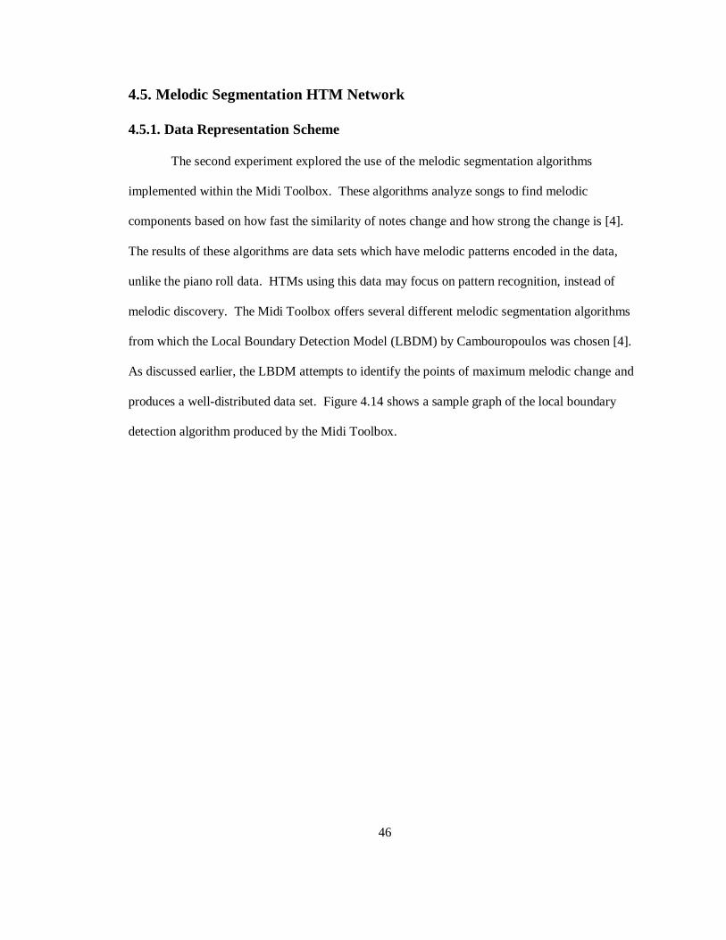
The second experiment explored the use of the melodic segmentation algorithms

implemented within the Midi Toolbox. These algorithms analyze songs to find melodic

components based on how fast the similarity of notes change and how strong the change is [4].

The results of these algorithms are data sets which have melodic patterns encoded in the data,

unlike the piano roll data. HTMs using this data may focus on pattern recognition, instead of

melodic discovery. The Midi Toolbox offers several different melodic segmentation algorithms

from which the Local Boundary Detection Model (LBDM) by Cambouropoulos was chosen [4].

As discussed earlier, the LBDM attempts to identify the points of maximum melodic change and

produces a well-distributed data set. Figure 4.14 shows a sample graph of the local boundary

detection algorithm produced by the Midi Toolbox.

47

Figure 4.14: Graph of the local boundary detection algorithm.

An examination of the local boundary detection data indicates sufficient variance and

hence appropriateness for use in a HTM network. However, before a data set could be created, a

transformation algorithm to convert a continuous graph along the time axis into a series of data

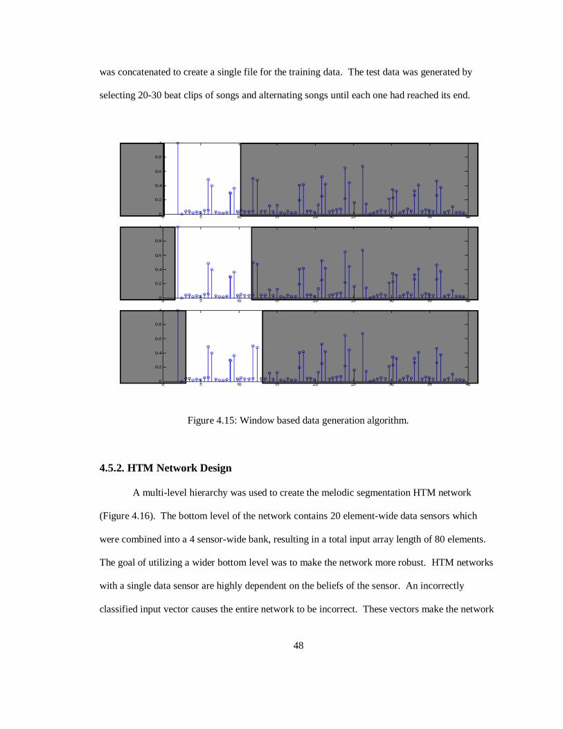
vectors needed to be developed. To perform this translation a window based approach was used.

Imagine a window of size 20 was placed on the graph which only allows one to see data from

time 1 to 20. As time continues to increase, the window slowly moves from left to right across

the graph. During each iteration, the data values within the window were recorded and placed in

a 20 element wide data vector. Figure 4.15 illustrates this algorithm graphically. This algorithm

was chosen because it encoded time into the data set, making up for NuPIC‟s lack of time-based

pattern inference. Five songs were chosen for the initial data set and the data from each window

0 5 10 15 20 25 30 35 40

G2

C3

F3

A3#

D4#

G4#

C5#

F5#

Time in beats

Pitch

ch1

ch2

0 5 10 15 20 25 30 35 400

0.2

0.4

0.6

0.8

1

48

was concatenated to create a single file for the training data. The test data was generated by

selecting 20-30 beat clips of songs and alternating songs until each one had reached its end.

Figure 4.15: Window based data generation algorithm.

4.5.2. HTM Network Design

A multi-level hierarchy was used to create the melodic segmentation HTM network

(Figure 4.16). The bottom level of the network contains 20 element-wide data sensors which

were combined into a 4 sensor-wide bank, resulting in a total input array length of 80 elements.

The goal of utilizing a wider bottom level was to make the network more robust. HTM networks

with a single data sensor are highly dependent on the beliefs of the sensor. An incorrectly

classified input vector causes the entire network to be incorrect. These vectors make the network

49

volatile and cause the top level belief to rapidly change. HTM networks with a wide base

minimize the impact of an incorrect bottom node belief because the remaining nodes are able to

override the incorrect node using belief propagation. Increasing the height of the HTM also

improves network stability. One of the underlying principles of HTMs is that low level nodes

encounter rapidly changing data and will quickly change beliefs, while higher level nodes have

more stable beliefs [7]. Increasing the height of the network takes advantage of this principle and

increases the likelihood of network stability.

Figure 4.16: Melodic segmentation HTM network structure.

50

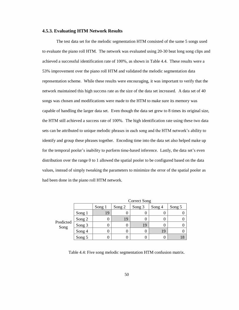
4.5.3. Evaluating HTM Network Results

The test data set for the melodic segmentation HTM consisted of the same 5 songs used

to evaluate the piano roll HTM. The network was evaluated using 20-30 beat long song clips and

achieved a successful identification rate of 100%, as shown in Table 4.4. These results were a

53% improvement over the piano roll HTM and validated the melodic segmentation data

representation scheme. While these results were encouraging, it was important to verify that the

network maintained this high success rate as the size of the data set increased. A data set of 40

songs was chosen and modifications were made to the HTM to make sure its memory was

capable of handling the larger data set. Even though the data set grew to 8 times its original size,

the HTM still achieved a success rate of 100%. The high identification rate using these two data

sets can be attributed to unique melodic phrases in each song and the HTM network‟s ability to

identify and group these phrases together. Encoding time into the data set also helped make up

for the temporal pooler‟s inability to perform time-based inference. Lastly, the data set‟s even

distribution over the range 0 to 1 allowed the spatial pooler to be configured based on the data

values, instead of simply tweaking the parameters to minimize the error of the spatial pooler as

had been done in the piano roll HTM network.

Correct Song

Song 1 Song 2 Song 3 Song 4 Song 5

Predicted

Song

Song 1 19 0 0 0 0

Song 2 0 19 0 0 0

Song 3 0 0 19 0 0

Song 4 0 0 0 19 0

Song 5 0 0 0 0 18

Table 4.4: Five song melodic segmentation HTM confusion matrix.

51

Chapter 5

DISCUSSION

5.1. Analysis of HTM Node Algorithms

While the melodic segmentation HTM network has proven that NuPIC can be used to

solve a traditional artificial intelligence problem, several limitations of HTM networks were

discovered along the way. The first experiment exposed a weakness in the spatial pooler‟s

Gaussian distance function when data is represented in a binary format. The function does not

take an element‟s position within the data vector into account and thus is unable to distinguish

between inputs such as 100001 and 000110, as shown below:

Distance between 100001 and 000000

Distance between 000110 and 000000

Figure 5.1: Position error in the spatial pooler.

52

Even though the Bitworm tutorial provided by NuPIC used a similar binary encoding scheme, the

weakness was not exposed because the HTM was trained to identify a limited amount of vastly

different patterns. The piano roll data set was more complex and had a large amount of subtle

patterns. In order to overcome this error in the spatial pooler, a more complex distance function

that takes element position into account needs to be developed. NuPIC already allows developers

to configure the spatial pooler when creating the network and it would be relatively simple to

allow developers to specify a special purpose distance function based on their data set.

Researchers would then be able to examine their data set and decide which distance function is

applicable.

Although NuPIC has a temporal pooler for time dependent patterns, it is only used when

training the network. During training the temporal pooler creates temporal groups based on

which quantization points occur near each other in time. Once the network is switched to

inference mode the HTM outputs the temporal group that contains the quantization point

produced by the spatial pooler, which allows for no time based inference [1]. Time based

inference allows a network to remember what it has previously seen and improves recognition

results [1]. As Figure 5.2 displays, time is essential to recognize certain types of patterns,

especially when there is a large amount of noise in the data. The melodic segmentation data set

overcame this shortcoming by using data that contained very little noise and encoding time into

the data set via sliding windows. However, in order for HTMs to be effective with more

complicated data, an algorithm for time based inference must be developed.

53

Figure 5.2: Difficultly of recognizing patterns in noisy data [1].

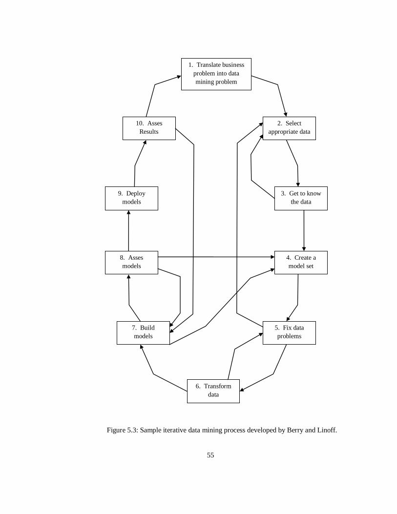
5.2. Development Process

A significant portion of this research was spent studying and pre-processing data sets

before they could be fed into HTM networks. Due to the project‟s focus on developing song

identification experiments, it wasn‟t until the end of the research that the importance of this step

in the NuPIC development process was realized. Upon investigation into the topic it was

discovered that the field of data mining also spends a large amount of time developing and

refining data. A brief survey of data mining literature revealed robust processes for refining data

and training data mining systems [2]. A large amount of the processes were also iterative due to

the uncertain nature of data mining. Figure 5.3 displays a popular data mining process developed

by Berry and Linoff [2]. After comparing the informal process created for HTM network

development to several popular data mining processes, a surprising amount of similarities were

found. Both processes require researchers to understand and pre-process data in order to

54

eliminate any problems with the learning algorithms. If HTM researchers wish to increase their

likelihood of success, they should look for ways to incorporate the data mining community‟s

knowledge into their research.

55

1. Translate business

problem into data

mining problem

2. Select

appropriate data

6. Transform

data

7. Build

models

8. Asses

models

5. Fix data

problems

4. Create a

model set

3. Get to know

the data

10. Asses

Results

9. Deploy

models

Figure 5.3: Sample iterative data mining process developed by Berry and Linoff.

56

5.3. Data Set Format

NuPIC has a partition-based data format for files read into HTM networks. The current

specification calls for input vectors to be placed into the data file one line at a time, with elements

separated by a single space [1]. If a category file is being used, a separate file must be used

where a single category number is placed on each line, corresponding to the line number in the

data file [1]. Maintaining data across two separate files and making sure line numbers match is a

cumbersome process, forcing large amounts of formatting code to be written in the data

generation scripts. It is also difficult for multiple data files to be read and combined. In order to

fix these problems NuPIC needs to switch to a XML based data input scheme, enabling freely

available XML toolkits to be used when writing data generation scripts. This format would allow

input vectors and category data to be combined into one file, hence making the data set easier to

maintain. A XML based data format would also enable researchers to develop schemas and

validate their data before the HTM is executed. Validation would reduce overall development

time by reducing data formatting errors, which are currently found only at run time.

5.4. Future Work

When evaluating NuPIC it is important to remember the software is still in its infancy.

As this research illustrates, NuPIC can be used to tackle more complex problems and researchers

need to continue to push NuPIC to its limits. The majority of current research is focused on

extending existing NuPIC tutorials to solve very detailed problems. While this is important,

researchers also need to focus on widening the number of problems NuPIC can be used to solve.

A crucial tool in increasing the scope of HTM research is time based inference. Late in this

research NuPIC version 1.5 was released which includes a time based inference algorithm [1].

Now that NuPIC has delivered this important feature, researchers need to make sure that their

57

data set gives them the ability to test the algorithm. It would also be interesting to see how this

algorithm would perform if the amount of temporal information encoded in the melodic

segmentation data set was minimized.

While this research indicates that NuPIC is not ready to handle a complex sample based

audio file format, it would be worthwhile to see how HTMs perform using multiple features.

While attempting to find a Midi file analysis toolkit, a tool for Midi file feature extraction tool

called JSymbolic was discovered [13]. This tool allows developers to extract a wide range of

features from the Midi files and is highly configurable. Data produced from this tool could then

be used to train a HTM designed for song identification. Combining multiple features could also

enable HTM researchers to move beyond the song identification problem and focus on a more

complex problem like genre classification.

58

BIBLIOGRAPHY

[1] “Advanced NuPIC Programming”, Numenta Incorprated, September 2007. [Online].

Available: http://www.numenta.com/for-developers/software/pdf/nupic_prog_guide.

[Accessed: October 2007].

[2] Berry, Michael and Gordon Linoff, Data Mining Techniques, Indianapolis: Wiley

Publishers Incorporated, 2004.

[3] Cambouropoulos, Emilos. “Musical Rhythm: A Formal Model for Determining Local

Boundaries, Accents, and Metre in a Melodic Surface”, in Music, Gestalt, and Computing,

Berlin: Springer, 1997, pp. 277-293.

[4] Eerola, Tuomas and Petri Toiviainen, “MIDI Toolbox: MATLAB Tools for Music

Research”, 2004. [Online]. Available: http://www.jyu.fi/hum/laitokset/musiikki/en/research/coe/materials/miditoolbox/.

[Accessed: January 2008].

[5] Dileep, George and Bobby Jaros, “The HTM Learning Algorithms”, Numenta Incorprated,

March 1, 2007. [Online]. Available:

http://www.numenta.com/for-developers/education/Numenta_HTM_Learning_Algos.pdf.

[Accessed: November 2007].

[6] Hawkins, Jeff and Sandra Balkeslee, On Intelligence, New York : Owl Books, 2004.

[7] Hawkins, Jeff and Dileep George, “Hierarchical Temporal Memory: Concepts, Theory, and

Terminology”, Numenta Incorprated , March 27, 2007. [Online]. Available:

http://www.numenta.com/Numenta_HTM_Concepts.pdf. [Accessed: October 2007].

[8] “Installing the Numenta Platform for Intelligent Computing”, Numenta Incorprated .

[Online]. Available: http://www.numenta.com/for-developers/education/installing-

nupic.php. [Accessed: October 2007].

[9] “The International Music Informatio Retrieval (MIR) and Music Digital Library (MDL)

Evaluation Project”, The University of Illinois, April 7, 2007. [Online]. Available: http://www.music-ir.org/evaluation/. [Referenced: February 2008].

59

[10] Lepple, Charles, “The Fast Fourier Transform Demystified”, May 13, 1996. [Online].

Available: http://www.ghz.cc/charles/fft.pdf. [Referenced: November 2007].

[11] Logan, Beth, “Mel Frequency Cepstral Coefficients for Music Modeling”, University of

Massachusetts, 2000. [Online]. Available: http://ciir.cs.umass.edu/music2000/papers/logan_abs.pdf. [Referenced: January 2008].

[12] McKay, Cory, “Automatic Genre Classification of MIDI Recordings”, Sourceforge, June 2004. [Online]. Available:

http://jmir.sourceforge.net/publications/MA_Thesis_2004_Bodhidharma.pdf. [Referenced:

December 2007].

[13] McKay, Cory and Ichiro Fujinaga, “jSymbolic: A Feature Extractor for MIDI Files”,

Sourceforge, 2006. [Online]. Available:

http://jmir.sourceforge.net/publications/ICMC_2006_jSymbolic.pdf. [Referenced: December 2007].

[14] “Pictures Demonstration Program”, Numenta Incorporated, 2007. [Online]. Available: http://www.numenta.com/about-numenta/technology/pictures-demo.php. [Referenced:

October 2007].

[15] “Problems That Fit HTMs”, Numenta Incorporated, March 1, 2007. [Online]. Available:

http://www.numenta.com/for-developers/education/ProblemsThatFitHTMs.pdf.

[Referenced: March 2007].

[16] Tzanetakis, George, Perry Cook, and Georg Essl, “Musical Genre Classification of Audio

Signals” IEEE Transactions on Speech and Audio Processing, vol. 10, no. 5, pp. 293-302,

July 2002.

[17] “Vitamin D Toolkit Reference Guide”, Vitamin D Incorporated, October 23, 2007.

Available:

http://www.vitamindinc.com/downloads/Vitamin%20D%20Toolkit%20Reference%20Guide.pdf. [Referenced: November 2007].

[18] “WAVE PCM Soundfile Format”, class notes for EE 367C, Electrical Engineering Department, Stanford University, Winter 2006. [Online]. Available:

http://ccrma.stanford.edu/courses/422/projects/WaveFormat/. [Available: October 2007.]