REPORT DOCUMENTA OBN.00 8

Ia. REPORT SFCURITY CLASSIFICATION

UNCLASS IFIED _)_T_1_(7________71

~AD-A212 7182. SECURITY CLASSIFICATION AUTH -- T-2b. DECLASSIFICATIONIDOWNGRA 4 CT E 9 1"39

198.9l I aiS.rIDuEion unLmicea.

4. PERFORMING ORGANIZATION R9 )R1,%UMBER(S) S. MONITORING ORGANIZATION REPORT NUMBER(S)

AE 06 -. IX. 9_ -- 1 0 3 2

6a. NAME OF PERFORMING ORGANIZATION 6b. OFFICE SYMBOL 7a. NAME OF MONITORING ORGANIZATION

ASA~ Lk NiMj 0(fR L CKI ______ Air Force Office of SCiantifiC~ RP~APreh6c. ADDRESS (City Slate, and ZIP Code) ,- 7b. ADDRESS (City, State, and ZIP Code)Tr4 4 .'u U jL)nl 1 " I IJ Cj"' Building 410

I I i ,4 , j Bolling AFB, DC 20332-6448

8a. NAME OF FUNDING/SPONSORING 8b. OFFICE SYMBOL 9. PROCUREMENT INSTRUMENT IDENTIFICATION NUMBERORGANIZATION (If applicable)

AFOSR I NM A SOSS k Q3-C-Sc. ADDRESS (City, State, and ZIP Code) 10. SOURCE OF FUNDING NUMBERS

Building 410 PROGRAM PROJECT TASK WORK UNIT

Bolling AFB, DC 20332-6448 ELEMENT NO. NO. NO 1 ACCESSION NO.

I 61102F 2304 /311. TITLE (Include Security Classfication)

12. PERSONAL AUTHOR(S) I

l C - e r_\_ S I'rC I .~~t rU k C (, / C I I v-jC (1. 'Ycu")13a. TYPE OF REPORT 13b. TIME COVERED 14. DATE'OF REPORT (Year, Month, Day) 15. PAGE COURAT

-J L FROML-J - TO3 -J-I I16. PPLEMENTARY NOTATION

17. COSATI CODES 18. SUBJECT TERMS (Continue on reverse if necessary and identify by block number)FIELD GROUP SUB-GROUP

19. ABSTRACT (Continue on reverse if necessary and identify by block number)

This effort supported the research activities of 20 researchers during theirvisit to ICASE, as a result, 10 papers have appeared on issues related toparallel computation including such titles as *Reordering computations forparallel execution',*"Multiprocessor L/U decomposition with controlledfill-in, and "Analysis of a parallelized nonlinear elliptic boundary valueproblems solver with applications to reacting flows .ll -1

20. DISTRIBUTION/AVAILABILITY QF ABSTRACT 21. ABSTRACT SECURITY CLASSIFICATION]UNCLASSIFIED/UNLIMITED 1jSAME AS RPT. C3 DTIC USERS UNCLASSIFIED

22a. NAME OF RESPONSIBLE INDIVIDUAL 22b. TELEPHONE (Include Area Code) 22c. OFFICE SYMBOL

14, C0 1 Ae1, , .i 1k (202) 767- ..DO Form 1473, JUN 86 Previous editions are obsolete. SEC IILS$1AGAA20096tIS PAGE

89

NASA Contractor Report 178212

ICASE REPORT NO. 86-8189-1032

ICASEANALYSIS OF THE SOR ITERATION FOR THE 9-POINT LAPLACIAN

/-

Loyce M. Adams

Randall J. LeVeque

David H. Young

Contract No. NASI-18107 L: --,

December 1986

INSTITUTE FOR COMPUTER APPLICATIONS IN SCIENCE AND ENGINEERING

NASA Langley Research Center, Hampton, Virginia 23665

Operated by the Universities Space Research Association

and

HOmv00 VYrgms23665

ANALYSIS OF THE SOR ITERATION FOR THE 9-POINT LAPLACIAN

Loyce M. Adams+

University of Washington

Randall J. LeVeque++

Uaiversity of Washington

David M. Young*

University of Texas at Austin

ABSTRACTS

The SOR iteration for solving linear systems of equations depends upon an

overrelaxation factor w. A theory for determining w was given by Young

[1950] for consistently ordered matrices. Here we determine the optimal w

for the 9-point stencil for the model problem of Laplace's equation on a

square. We consider several orderings of the equations, including the natural

rowwise and multicolor orderings, all of which lead to non-consistently

ordered matrices, and find two equivalence classes of orderings with different

convergence behavior and optimal w's. We compare our results for the

natural rowwise ordering to those of Garabedian [1956] and explain why both

results are, in a sense, correct, even though they differ. We also analyze a

pseudo SOR method for the model problem and show that it is not as effective

as the SOR methods. Finally, we compare the point SOR methods to known

results for line SOR methods for this problem.

This research was supported in part by NASA Contract NASI-18107 while thefirst and second authors were in residence at the Institute for ComputerApplications in Science and Engineering (ICASE), NASA Langley Research CenterHampton, VA 23665. Also, rescarch was rupported in part by AFOSR Contract

85-0189.

+ Research supported in part by AFOSR Grant No. 86-0154.

++ Research supported in part by NSF Grant No. DMS-8601363.Research supported in part by DOE Grant No. DE-A505-81ER10954, NSF Grant

No. MCS-821473, AFOSR Grant No. 85-0052.

• • • m |

1. Introduction.

The SOR method (successive overrelaxation) is a standard iterative method for solving linear

systems of equations, particularly large sparse systems arising from partial differential equations.

Convergence of the method is greatly affected by the choice of overrelaxation parameter (o. A stan-

dard model problem for analyzing SOR is the system of equations arising from a finite difference

discretization of Laplace's equation on a rectangle with zero boundary data. The solution of this prob-

lem is identically zero; hence, the iterates of SOR also represent the error at each step. The copver-

gence properties of SOR for the model problem also apply to Poisson's equation with general Dirichlet

boundary data, since the errors will still satisfy the homogeneous equation.

Using the five-point approximation to the Laplacian gives

uj-IR + uj+lk + jk-l + ujk+l -4ujk = 0, j,k = 1, 2, ,N-l,

uAk=O, j=O,N ork=0,N,

where ujk approximates the solution u (xj,yk) with x= jh, yk = kh, and h = 11N. This gives a linear

system of (N-1)2 equations in (N-) 2 unknowns. The exact form of the matrix equation, and the form

that the SOR iteration takes, depends on the order in which the unknowns ujk are arranged in the vec-

tor of unknowns. Two standard orderings are the natural rowwise (NR) ordering and the Red-Black

(RB) ordering, in which the grid is colored in a checkerboard fashion and the Red points are ordered

before the Black points (by rows within each color). For the model problem, the optimal co and rate of

convergence are the same for both of these orderings. This mode. )-b em was analyzed by

Frankel[1950] and also by Young[1950] who gave a more general theory )R for a wide class of

matrix equations in which the matrix is "consistently ordered".

Another standard model problem is obtained by using the nine-point approximation to the Lapla-

cian:

4uy-tt + 4 U,+I.k + 4 uJ,k-I + 4uj.4.1 + Ui-.kl- + uj-L +l

+U++u +t,,+1-2Ouy =O, j, k = 1,2, 1, (1.2)

Uk-O, j=O,N ork=O,N

2

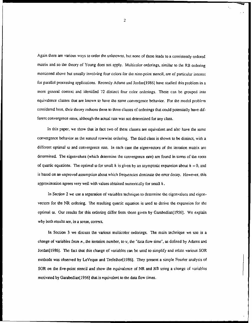
Again there are various ways to order the unknowns, but none of these leads to a consistently ordered

matrix and so the theory of Young does not apply. Multicolor orderings, similar to the RB ordering

mentioned above but usually involving four colors for the nine-point stencil, are of particular interest

for parallel processing applications. Recently Adams and Jordan[1986] have studied this problem in a

more general context and identified 72 distinct four color orderings. These can be grouped into

equivalence classes that are known to have the same convergence behavior. For the model problem

considered here, their theory reduces these to three classes of orderings that could potentially have dif-

ferent convergence rates, although the actual rate was not determined for any class.

In this paper, we show that in fact two of these classes are equivalent and alse have the same

convergence behavior as the natural rowwise ordering. The third class is shown to be distinct, with a

different optimal (o and convergence rate. In each case the eigenvectors of the iteration matrix are

determined. The eigenvalues (which determine the convergence rate) are found in terms of the roots

of quartic equations. The optimal (o for small h is given by an asymptotic expansion about h = 0, and

is based on an unproved assumption about which frequencies dominate the error decay. However, this

approximation agrees very well with values obtained numerically for small h.

In Section 2 we use a separation of variables technique to determine the eigenvalues and eigen-

vectors for the NR ordering. The resulting quartic equation is used to derive the expansion for the

optimal (o. Our results for this ordering differ from those given by Garabedian[1956]. We explain

why both results are, in a sense, correct.

In Section 3 we discuss the various multicolor orderings. The main technique we use is a

change of variables from n, the iteration number, to v, the "data flow time", as defined by Adams and

Jordan[1986]. The fact that this change of variables can be used to simplify and relate various SOR

methods was observed by LeVeque and Trefethen[1986]. They present a simple Fourier analysis of

SOR on the five-point stencil and show the equivalence of NR and RB using a change of variables

motivated by Garabedian[1956] that is equivalent to the data flow times.

3

In Section 4 we analyze a pseudo-SOR method based on a Red-Black coloring for the nine-point

stencil. Although this method has attractive features for parallel computers, we show that it is unsatis-

factory, being an order of magnitude slower than the true SOR methods with optimal w.

Finally, in Section 5, we briefly discuss line SOR methods and compare their convergence rates

with the point SOR methods discussed in this paper.

2. Analysis of the natural rowwise ordering.

For the nine point stencil with NR ordering, the SOR method takes the form

Uji+I = (l-(1) s + (UI 1+u 1 un (2.1)

+ k - 5 j( j7+UJ i+U j+lt+Ujk+l)(

(U 1o "U j - l1k - 1 "t )+ j k + ! -bU j'+ l k - 1 ]

We assume that this iteration has a solution of the form

u11 = X MW(xjyk). (2.2)

Then X is an eigenvalue of the iteration matrix and the vector with components

w(xj,yk), jk = 1, .- -, N-1 gives the corresponding eigenvector. Plugging (2.2) into (2.1), cancel-

ling a common factor of V", and dropping the subscripts on x and y gives

XW (x ,y) = XO I -ly)+-Lw ,y (x-hy-h)+w(x ,y-h)+-Lw (x+h ,y-h)

+0) w(x+hy)+-(w(x-hy+h)+-w(xy+h)+ -w(x+hy+h) (2.3)

+ (1- 0o) w (x,y).

The eigenfunction w (x ,y) must be zero on the boundary of the unit square in view of the given boun-

dary conditions.

We use separation of variables and let w (x ,y) = X (x)Y (y). We also set IX = X112. Plugging this

into (2.3) and dividing by X(x)Y(y) gives

4

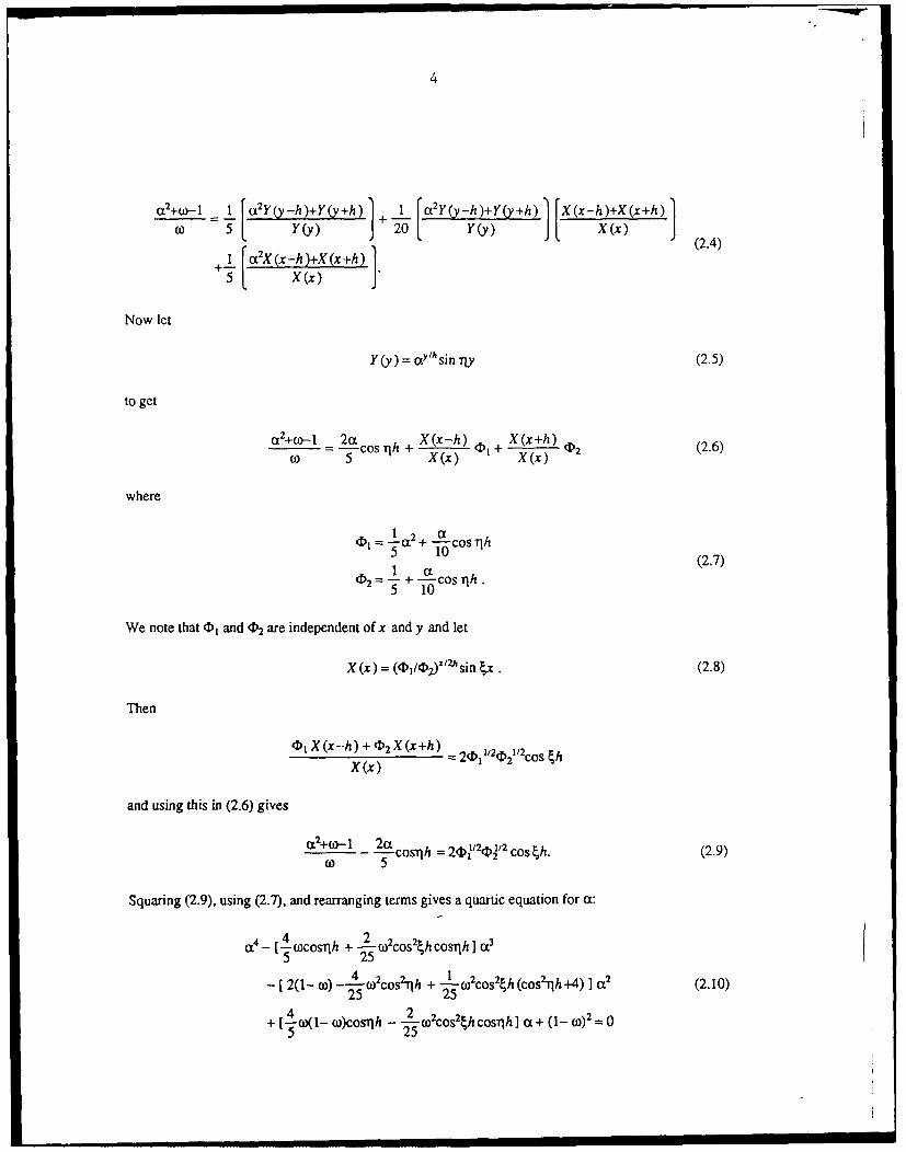
_+Gy-I 1 a2y(y-h)+Y(y+h) 1 I 2Y(y-h)+Y(y+h) X(x-h)+X(x+h)o =5Y~y) + Y(y) J X(x) J

I y() 1 20 Y()xX)(2.4)

1L co2X(x-h)+X(x+h) 15 x (X) J

Now let

Y(y) = ezy/hsin 71y (2.5)

to get

o+co--I _ 7h X(x-h) X(x+h)6S co -h + 2(2.6)

(0 5 X (x) X(x)

where

5 10 (2.7)

02 = a- + -- cos 71h.5 10

We note that b1 and 02 are independent of x and y and let

X (x) = ((i 1 /4)j)x/2I sin Ex. (2.8)

Then

(D X (x--h) + 2 X (x +h) 1 21/2

X (X)

and using this in (2.6) gives

2+(o-- _ 2a corh = 20 112( 1,2 cos th. (2.9)(2.91) 2

Squaring (2.9), using (2.7), and rearranging terms gives a quartic equation for a:

4 4 OCSh+2~ 622t oihI5 25

-t2(1- (-0)-4Ocosnh + -Lacos2 th(cos1h 44) 1 a2 (2.10)25 25

+4 (LI 1)O1h_- W2 h 22~ l a + (1_ W) 2 =05 ~ n 25 C sh

5

An eigenmode of the iteration matrix thus has the form

u, = XX (xj)Y.y) (2.11)= L2n+* [((sD)/4)j sin~x, sinlyk.

In order for the boundary conditions to be satisfied, k and rj must be integer multiples of it. The eigen-

value is X = o2 , where cc is a root of (2.10). Note that we must choose the correct square root of 01/02

in (2.11) (recall that we squared (2.9) to obtain (2.10), introducing additional solutions). The correct

sign for @1/2 I2 is determined by the requirement that (2.9) be satisfied, and this gives the correctsign for 12 / D12 as well.

The frequencies t and TI each range over the values t, 21t, •, (N-1)2. This gives a set of

(N-1)2/4 pairs of frequencies. Corresponding to each pair (4jj) there are four roots of the quartic

(2.10). In general these roots are distinct, and so we obtain (N-1)2 eigenvalues and eigenvectors, the

correct number. When the roots are not distinct, principal vectors will be obtained and the number of

eigenvectors will be less than (N-) 2 . Recall that for the 5-point discretization, a principal vector was

associated with the optimal o, (see e.g. Young[1971]). We make no attempt here to determine the

principal vectors or the values of a) for which they occur. However, by continuity, we do obtain all of

the eigenvalues.

The frequencies ( -1 +l)n, " , (N-1)nt, which one might expect to be included as well, give

repeats of the eigenvectors already found. Replacing 4 by Nit-4 leaves (2.10) unchanged while

replacing TI by Ni-T1 simply negates the coefficients of a and a 3. In either case the squares of the

roots are unchanged. The eigenmodes (2.11) are also unchanged by these frequency reflections.

The convergence rate of the method (for fixed o) is determined by the spectral radius of the

iteration matrix, which is

p to max I over (.

To determine the optimal (o, we need to minimize p over wo.

6

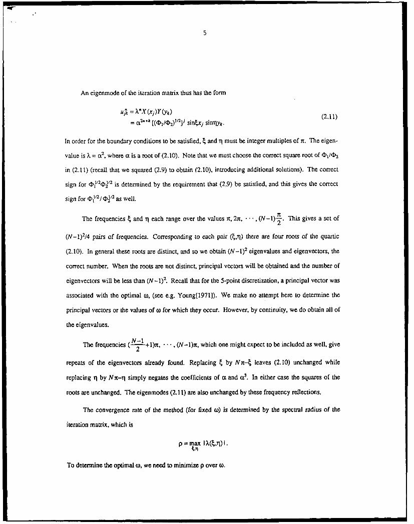
To help characterize the roots of (2.10), we first solved the quartic numerically for various

values of the parameters. For example, the solid lines in Figure 2.1 (the x's will be explained later)

show the magnitude of the four roots plotted as a function of o when -r--r for h=1/10, 1/100, and

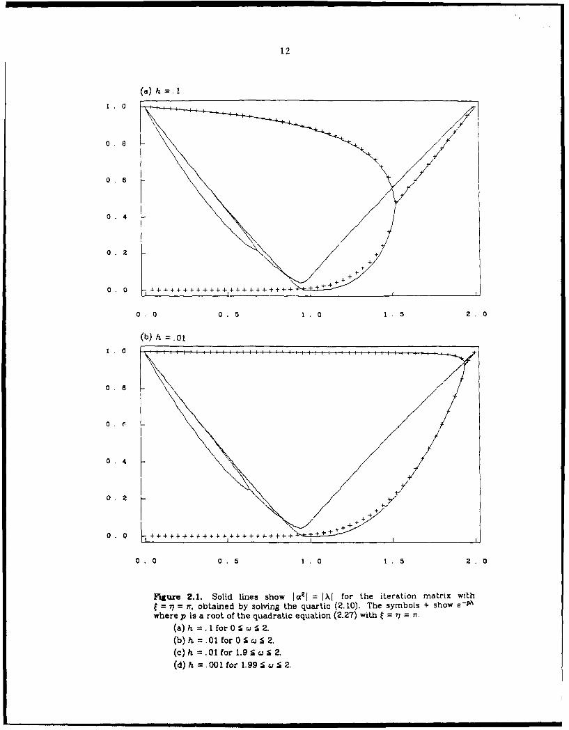
1/1000. When co is small there are four real roots. As (o increases, two of the roots become complex

conjugates. The optimal (o apparently occurs when these complex roots intersect the largest real root.

As omega increases further, two more roots become complex conjugates and near o=2 there are two

complex conjugate pairs. The same behavior was observed for smaller values of h using various

values of and -q.

In all our experiments with various values of h, t----n produced the largest root at each co and

hence the optimal (o can presumably be determined by minimizing the roots for this particular combi-

nation of frequencies. This is consistent with what is known to be true for the five-point model prob-

lem, but we have not been able to prove that this is correct for the nine-point stencil.

These observations suggest a strategy for determining the optimal omega for small h when

=1-. We first find the roots of (2.10) when h = 0 and then expand about these roots and equate the

modulus of the roots to get the optimal o. As h -- 0, the optimal (o approaches 2. Setting h = 0 and

co = 2 in (2.10) gives

o: 48 t3 46t2_ 48(z--483 + - - +1 = 0. (2.12)25 25 25

The roots of (2.12) are

al=l, a2=l, c 3=e i e, ct=e-ie (2.13)

where O=cos- 1(-1/25).

First, we expand the real root at wcop about a,=l. We set

ca= 1-c1h -c 2h2 , (2.14a)

o=2-k lh -k 2h2 (2.14b)

and substitute into (2.10). After equating coefficients of h 2 we get

7

13c - l5kc + 18t 2 =0, (2.15)

..hich determines c1 as a function ofk .

Next we expand about e i, setting

a=ei( 1-Ph) (2.16)

and again take co of the form (2.14b). Substituting into (2. 10) and equating coefficients of h gives

144 92 2i 48 e k 10k128e 3i 4 6 e 2ie+ 68 iO-2) (2.17)13 (4e4' 8 - ~e~ie+ - ei) =kl-e i - -. ) (.

25 25 25 25 25 25

which determines 03 as a function of k 1:

13=.423077 k 1 . (2.18)

Recall that X= o2 is the eigenvalue we seek, so we equate I o2 I from (2.14a) and IctI from (2.16) to

highest order to get

1 -2c h +0(h 2 )= -213h +0(h 2),

and so c 1=13. Plugging this into (2.15) and using (2.18) allows us to solve for k1 ,

k1 =2.11624t. (2.19)

Consequently,

c .895337t. (2.20)

Using these values in (2.14a) and (2.14b), we find that the optimal (o and the corresponding spectral

radii have approximate values

oopt 2 - 2.11624rh

P1Pt = t = I - 2c h = 1- 1.790667rh

for small h.

For comparison, the corresponding values for the five-point model problem are

o 5--1' = 2 - 2th,

- • m l I It Ioptt

8

PrS-Pt = 1 - 2th.

Notice that for the nine-point stencil, the spectral radius is slightly larger, giving somewhat slower

convergence than for the five-point stencil, although the two are very close. Most importantly, both

are 1 - 0 (h) as h -- 0, giving asymptotically the same order of convergence. By contrast the Jacobi

and Gauss-Seidel methods, and also the pseudo-SOR method analyzed in Section 4, have spectral

radius 1 -O(h 2) ash -40.

It is very interesting to compare these results with asymptotic results obtained by Gara-

bcdian[1956], especially since they do not agree and yet both are, in a sense, correct. Garabedian's

analysis is based on viewing the SOR iteration (2.1) as a finite difference method for a time-dependent

PDE. Expanding in Taylor series shows that this difference equation is consistent with the PDE

5Cu, + 2u, + 3u, =3u, + 3 uy (2.22)

u =0 on the boundary

where C and w are related by

2 (2.23)

1+Ch

If we fix C >0 and choose o according to (2.23) for each h>0 then 0ko<2 and so the method (2.1) is

stable. Since it is consistent with the linear equation (2.22), iterates ujk with n=T/h must converge to

solutions u(xj,y,,T) of the PDE (2.22) as h-0 (by the Lax Equivalence Theorem) if we choose uk

by discretizing fixed initial data u (x,y ,0). Consequently, studying the decay of solutions to (2.22)

gives information about the rate of convergence of SOR.

By introducing the change of variables

I + L + (2.24)3 2

(2.22) is transformed to

5Cu, + -3u. = 3u. + 3u... (2.25)12

9

separation of variables shows that e,znmodes of this PDE have the form

u (x ,y ,s) = e -Psin x sin Tly (2.26)

where t and TI are integer multiples of t and p=p ( t,) is a root of the quadratic equation

13.2 5Cp + 3(_+ ) = 0. (2.27)

Transforming back to the original time variable gives

U (x ,y ,) = e (1+x3+y/2) sin kx sin lY-. (2.28)

Note that in a time step of length h, this solution decays by a factor e - R,(,)h. The eigenmode with

slowest decay is obtained by taking k=j--- and the negative square root in solving (2.27) giving

pin=' (f5C- .'25C.26t2] (2.29)

If we obtain initial data for SOR by discretizing the corresponding eigenfunction,

u =u (xj ykO) from (2.28), it follows (by convergence) that the decay factor for the SOR iteration

must have the form

I I - Re(p,. ,h + 0 (h2 ) (2.30)

as h -0. Since taking other eigenfunctions as initial data gives faster decay, one is led to the conclu-

sion that in order to obtain the fastest possible convergence, we should maximize Re (p ,) and hence

minimize X,,,. Recall that the value of C is still at our disposal. We can minimize Re (p ,,) by set-

ting the radical to zero in (2.29), giving

C = --2in = 1.02t, pi= 6, 4 2/03 = 2.35t. (2.31)

By (2.23) and (2.30) we obtain the following predictions for the optimal (o and the corresponding

decay rate, as in Garabedian[19561:

2 2(l-Ch) = 2 - 2.04rh1+Ch (2.32)

p3,t - e-/ -- I - p ,i,,h = I - 2.35nh .

10

These values do not agree with the values (2.21) found by computing the eigenvalues of the

iteration matrix. The reason is the following. While (2.30) does indeed give a correct expression for

the largest eigenvalue of the iteration matrix corresponding to a decay factor for the PDE, there are

other, spurious, eigenvalues of the discrete problem that have larger magnitude for o near 2 and hence

determine the spectral radius p. This is seen clearly in Figure 2.1 where we have plotted Ie-Ph I for

the two roots of the quadratic (2.27) (as +'s) along with I %I, the magnitudes of the actual eigenvalues

obtained by solving the quartic (2.10) (as the solid lines). One pair of discrete eigenvalues closely

matches l e -P I for small h while the other (complex conjugate) pair does not. In fact, Garabedian's

results may also be obtained from our approach by choosing k1 in (2.15) to maximize c 1, thereby

ignoring the effect of the other root.

For each fixed h, we can choose initial data (namely, as a spurious eigenvector) so that conver-

gence is slow and determined by the spectral radius. On the other hand, these spurious eigenvectors

become highly oscillatory and are not convergent as h -- 0. Consequently, if we obtain our initial data

by discretizing a fixed function of x and y at each h (as is more realistic in practice), we would expect

to see vanishingly small components of these spurious eigenvectors as h -*. For practical purposes,

then, the values (2.32) obtained by Garabedian may be more meaningful and useful than the "true"

values (2.21).

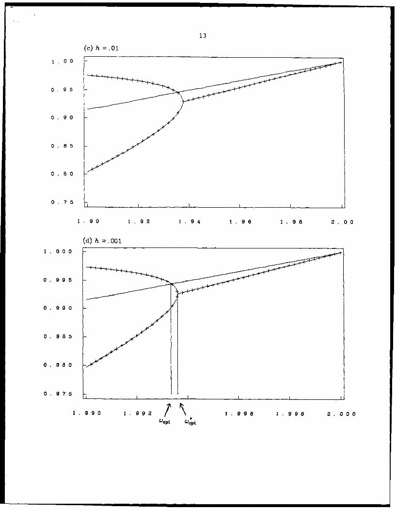
This is demonstrated in Figure 2.2 where we show the decay of I I u 112 for various initial data.

For initial data obtained by discretizing the smooth data u(x,y)=(x2-x)(y 2-y), the observed decay is

much closer to .,, as predicted by (2.30), than to p'.

To verify that the eigeave. tor corresponding to the spectral radius is highly oscillatory, we note

that by (2.5) and (2.8) an eigenverc hais the .,rm

o [(0r/)r'i]'sin ,xjsiny&. (2.33)

At the point op,, the maxim,-m eige, -.;ue corresponds to a value of a given by (2.16). Inserting this

in (2.33) gives

'I

wjk = e ie"(1 - 3)k [(l/@) 1 2]jsin xjsinrlyk. (2.34)

Since 0 cos-'(-1/25), this function will be oscillatory in k and nonconvergent as h -+ 0.

By contrast, the eigcnvector corresponding to the other pair of roots converges to the eigenfunc-

tions (2.28) of the PDE as h -4 0. For these vectors our previous arguments show that X has the form

of (2.30) and hence a, the square root of X, can be expressed as

I - ph + 0 (h 2). (2.35)2

Expanding 4)1/(D2 using this value of a in (2.7) shows that

(D1/D2 = 1 - -2ph + O(h 2). (2.36)

Plugging (2.35) and (2.36) into (2.11) gives

1 h 1 h

u =(1- -ph +O(h 2))2 n +k (1 - ph + O (h 2))j sin~jh sinrlkh (2.37)2 3

= (1 - ph + 0 (h 2)) +j/3+klsinkjh sinTlkh.

As h -+ 0 with t = nh, x = jh and y = kh fixed, this approaches the eigenmode (2.28) of the PDE.

12

(a) h = .10

o. 8

0.6 /0.4

0 0 4 + + +""4 + 4. +t 4"- 1+ + 4- +" + ++4+ I

0 . 2 5

(b) h 0.1o

1 0

0 4

1/+

0 .0 + I' 4 - +'4" 4. 4- + + + + + I I

0. 0 0. 5 1. 0 .5 2. 0

figure 2.1. Solid lines show Ja2I = JI for the iteration matrix with= 7 = nr, obtained by solving the quartic (2.10). The symbols + show e-P"

where p is a root of the quadratic equation (2.27) with t = 77 = I.(a) h = . I for 0 ;5 2.(b) h = .01 for 0 S 5 S 2.

(c) h =. 01 for 1.9 S ci S 2.

(d) h = .001 for 1.995 cj ; 2.

13

(c) h = .01

0.90

08 5

08 0

1.9 0 1.9 2 194 0.9 1.20

(d) h =.001

0. 00

0. 985

1.9 90 1.9 9.9 .98 2.0 00

14

1

10- 1

~(a)

(b)

i ~ ~~10-7

0 20 40 60 80 100 120 140 160

it erati on

Figure 2.2. Convergence history (2-norm of error versus iteration number) for theNR ordering with h = 0.05 and c = 1.86. Three choices of initial data are compared:

(a) An eigenvector corresponding to the spectral radius.(b) An eigenvector corresponding to the largest nonspurious eigenvalue.

(c) UjA = (XJ2 - X0)(Yt, - Yk ).Note that the realistic initial data (c) more closely matches (b) than (a).

15

3. Multicolor SOR.

In this section we consider the SOR method applied to the nine-point model problem with

several alternative orderings of the unknowns ujk. These orderings are determined by labeling the grid

points with four different colors (Red, Black, Green and Orange) and then ordering the points by first

listing all the points of one color, then a second color, and so on. The overall ordering of grid points is

determined by two factors: a) the manner in which the grid points are labeled (the coloring of the grid)

and b) the order in which the colors are taken (the ordering of the colors).

Four-colorings are of interest for the nine-point stencil because with four colors it is possible to

decouple the grid, in the sense that the resulting SOR formula for updating a grid point of any given

color involves neighboring grid points, all of which have different colors than the center point. This is

advantageous in parallel processing applications since all grid points of the same color can be updated

simultaneously.

For the five-point stencil, two colors suffice to decouple the grid using the RB checkerboard pat-

tern discussed in Section 1. Recently LeVeque and Trefethen[1986] have shown an easy way to

ana.yze the five-point model problem using a change of variables from the iteration number, n, to the

earliest time, v, that the unknown at a grid point can be updated assuming one update requires one time

unit. This variable v corresponds to the "data flow times" discussed in Adams and Jordan[1986] and

closely resembles the change of variables used by Garabedian[1956] to analyze the PDE. This change

of variables allows the use of Fourier analysis to determine the convergence rate and optimal . It

also gives a straightforward proof of the equivalence of the NR and RB orderings.

Here we use this same approach to analyze the four-color orderings for the nine-point stencil.

Before introducing these orderings, we briefly review the analysis for the five-point NR and RB order-

ings to introduce notation and motivate our nine-point analysis.

For the five-point model problem (1.1) with the NR ordering, the SOR iteration takes the form

Uj 1 =(1-0) uj + -u. "-luj7+lTu7+).0" (3.1)

4i u)I II-1 u 'k 1

16

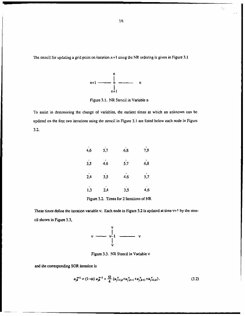
The stencil for updating a grid point on iteration n+1 using the NR ordering is given in Figure 3.1

n

In+I- n n

nil

Figure 3.1. NR Stencil in Variable n

To assist in determining the change of variables, the earliest times at which an unknown can be

updated on the first two iterations using the stencil in Figure 3.1 are listed below each node in Figure

3.2.

416 5,7 6,8 7,9

3,5 4,6 5,7 6,8

2,4 3,5 4,6 5,7

1,3 2,4 315 4,6

Figure 3.2. Times for 2 Iterations of NR

These times define the iteration variable v. Each node in Figure 3.2 is updated at time v+1 by the sten-

cil shown in Figure 3.3,

v

- v-I v

Figure 3.3. NR Stencil in Variable v

and the corresponding SOR iteration is

uj k+'- - (I--Wo)uj't + -2 (u V- ,*+UJ+iv + U +') (3.2)

4 J- .41+jI1+j+k

17

Figure 3.2 shows that the times along lines j+k are constant and that iterations in variable n occur

every 2 time units. Hence, the proper change of variables between (3.1) and (3.2) is

v=2n +-j +k -2. (3.3)

The advantage of this change of variables is that the eigenmodes of (3.2) are easy to determine -

they are simply Fourier modes of the form

uv = g sinxj sinrlyk. (3.4)

These grid functions satisfy the boundary conditions provided that 4 and in are integer multiples of it,

and substituting into (3.2) gives the following equation for g:

g2 = (I-W) + -(cos~h +cos'h). (3.5)

2

For each 4 and I, this equation has two solutions, giving two eigenmodes. We obtain all modes by let-

ting and Tj range over the values 4, 1 = it, 21t ... , (N-1)it, for a total of 2(N-1)2 modes. This is

correct since (3.2) requires two previous levels of data to calculate uji t

By the change of variables (3.3), an eigenvalue X of (3.1) is seen to be g 2 and the corresponding

eigenvector has components gj+ksin xj sinrlyk. We now appear to have twice as many eigenmodes

as required for (3.1), but here each mode is repeated since replacing (4,1) by (Nit-4, N -i) simply

negates the roots of (3.5). Since X = g 2 this reflection leaves these eigenvalues unchanged. The eigen-

vector is also unchanged since

(-g)j+ksin(N t--)xj sin(N t-rl)yk = g I+ksinjxj sinflyk.

Equation (3.5) gives the famous relationship between an eigenvalue X of SOR and an eigenvalue

W-=- (cos~h+cos1h) of Jacobi:

(3.6)

Equation (3.6) can be used to determine the optimal value of W as a function of 4± (see e.g.

Young[19711) and will not be repeated here.

18

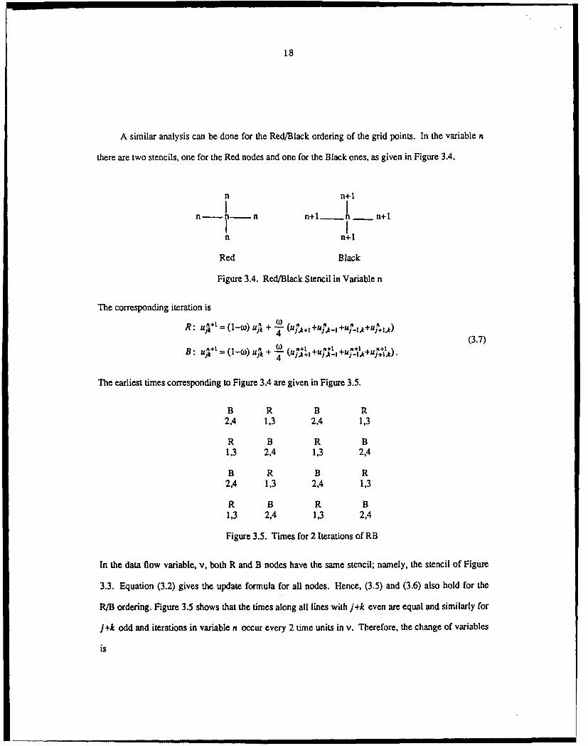
A similar analysis can be done for the Red/Black ordering of the grid points. In the variable n

there are two stencils, one for the Red nodes and one for the Black ones, as given in Figure 3A.

n n+1ri- - n+I- - n+l

n n+1

Red Black

Figure 3.4. Red/Black Stencil in Variable n

The corresponding iteration is

R : .u,,1= (1-o)uJ + to( " " " +?+u'..AuAR : jk' =( O Ujk, + - (UJ11 'l+ Ujk-l + U i-l'k+ UJ '1k)

(3.7)

B: U'+=(1-(o) UA + to (,.++ul .Jk-+ _+ k+"1V*J4 T d l"'a k- j lkvj+l~k) "

The earliest times corresponding to Figure 3A are given in Figure 3.5.

B R B R2,4 1,3 2,4 1,3

R B R B1,3 2,4 1,3 2,4

B R B R2,4 1,3 2,4 1,3

R B R B1,3 2,4 1.3 2,4

Figure 3.5. Times for 2 Iterations of RB

In the data flow variable, v, both R and B nodes have the same stencil; namely, the stencil of Figure

3.3. Equation (3.2) gives the update formula for all nodes. Hence, (3.5) and (3.6) also hold for the

R/B ordering. Figure 3.5 shows that the times along all lines with j+k even are equal and similarly for

j+k odd and iterations in variable n occur every 2 time units in v. Therefore, the change of variables

is

19

v=2n +(j+k) mod2- 1 (3.8)

and the eigenvector components of this iteration corresponding to t,TI are

Wjk sin~xyinlyA:wk = { sinxjsiny

for the R and B nodes respectively. This agrees with that given in Young[19501.

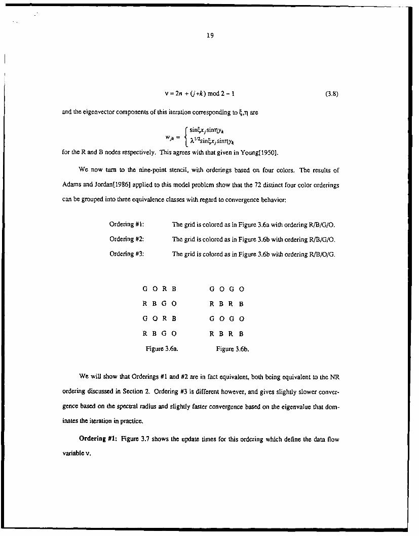
We now turn to the nine-point stencil, with orderings based on four colors. The results of

Adams and Jordan[1986] applied to this model problcm show that the 72 distinct four color orderings

can be grouped into three equivalence classes with regard to convergence behavior:

Ordering #1: The grid is colored as in Figure 3.6a with ordering R/B/G/O.

Ordering #2: The grid is colored as in Figure 3.6b with ordering R/B/G/O.

Ordering #3: The grid is colored as in Figure 3.6b with ordering R/B/O/G.

G O R B G OG O

R B G O R B R B

G OR B G OG O

R B G O R B R B

Figure 3.6a. Figure 3.6b.

We will show that Orderings #1 and #2 are in fact equivalent, both being equivalent to the NR

ordering discussed in Section 2. Ordering #3 is different however, and gives slightly slower conver-

gence based on the spectral radius and slightly faster convergence based on the eigenvalue that dom-

inates the iteration in practice.

Ordering #1: Figure 3.7 shows the update times for this ordering which define the data flow

variable v.

20

G 0 R B3,7 4,8 1,5 2,6

R B G 01,5 2,6 3,7 4,8

G 0 R B3,7 4,8 1,5 2,6

R B G 01,5 2,6 3,7 4,8

Figure 3.7. Times for two iterations with Ordering #1

In this variable, each node has the same stencil with update formula

u = (1- w)u + - - (uUj+2

+ 1 +(3.9)

20 j j--I uj-l, k+l+U73 j+lk-+Uj +l).

The change of variables is given by

v=4n +c -3 (3.10)

where c = 0, 1, 2, 3 for the R, B, G, and 0 nodes of Figure 3.7, respectively.

To see that this ordering is equivalent to the NR ordering, we only need to look at the update

times for the NR ordering, shown in Figure 3.8.

7,11 8,12 9,13 10,14

5.9 6,10 7,11 8,12

3,7 4,8 5,9 6,10

115 2,6 3,7 4,8

Figure 3.8. Times for the 9 point NR Ordering

If we define the variable v by these times, we again obtain iteration (3.9) with the change of variables

21

v=4n +2k +j -6. (3.11)

Since a change of variables gives (3.9) in either case, the eigenvalues and hence convergence behavior

will be identical. If g is an eigenvalue of (3.9) then X = g 4 is an eigenvalue of both NR and Ordering

#1.

The eigenvectors, however, will not be the same since a different change of variables is used in

each case. The eigenvectors for the NR ordering were determined in Section 2. Using these and the

above changes of variables allows us to determine the eigenvectors for Ordering #1. In analyzing (3.9)

we view it as applying to all mesh points (j,k) at each level of v, although in our applications it is

applied only to points of a single color in each step. (Note that we could apply it to all points without

affecting the results, but that the work required would be increased by a factor of 4.) Since (3.9)

requires four levels of prior data to determine u1' 4 , an eigenvector of (3.9) consists of 4(N-1) 2 values,

[V0]

VIV = V 2

v3

where Vv = VV for j, k , 2,. • , N-1. If g is the corresponding eigenvalue, then

V2 V1

V3 = g V2 •

0 VW

This indicates that V" +' = gV" for each v and hence

VO]gV 0

Sg2V0 I R 4(N- 1).

93,O

If we now let V°' be the vector consisting only of the values Vj for which (jk) is a red point, and

similarly for V° , V° and V°, then an eigenvector of the original iteration in the n variable (with Ord-

ering #1) has the form

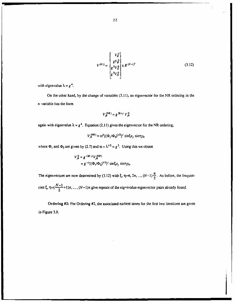
22

#(3.12)

with eigenvalue X g4.

On the other hand, by the change of variables (3.11), an eigenvector for the NR ordering in the

n variable has the form

ViNR) =g2+j Vo

again with eigenvalue X= g4. Equation (2.11) gives the eigenvector for the NR ordering,

V )=R) = ak[( Q/1 2)]'2] sin~xj sinTlyk

where Z> and 02 are given by (2.7) and a = X -1 = g 2. Using this we obtain

V,2k g 2kVVir )

= g- [(d'/(D211 2] j sin,xj sinTlyk.

The eigenvectors are now determined by (3.12) with t, Tl---n, 21, ..., (N-)-. As before, the frequen-2

cies 4, Tl=(- +l)ir, ... (N-1)m give repeats of the eig-nvalue-eigenvector pairs already found.2

Ordering #2: For Ordering #2, the associated earliest times for the first two iterations are given

in Figure 3.9.

23

G 0 G 03,7 4,8 3,7 4,8

R B R B1,5 2,6 1,5 2,6

G 0 G 03,7 4,8 3,7 4,8

R B R B1,5 2,6 1,5 2,6

Figure 3.9. R/B/G/O Times for Ordering #2

A quick inspection of Figure 3.9 shows that the R and G nodes have the same stencil in the variable v

with the following update formula:

= (1 _ (, v+1 j. v+ l .. v+2 , v+2

R,G: u + = (1- co) u.+-( " +u'-lJ:-uk l-l-j,5 _ 1 j k- h +I (3.13)

+ -2!- (U v+3 3v+3 Jv-+3 +U v+3

20 j-lk-lrj-lk+lruj+l,*-lrj~lk+l

Likewise, the B and 0 nodes have the same stencil with update formula:

B O: u 1+ = (1_ W) U- o!U ,+3 +U -3 +U +2 + +V+2

A Jkr 5 V j-lk UJ+l k T j~k-I 'Jk+l ( .4Uj~+~yUj..I(3.14)

+ o t jv+ l' - -U v + l -- V + 1 , v + l "

2 0 , U -A -+ j -, k + l + U j + l ,k - -, ', j + lI A + I ) .

The change of variables from n to v is again given by (3.10), where c = 0, 1, 2, and 3 for the R, B, G,

and 0 equations respectively.

Now, the equations in (3.13) and (3.14) have the symmetry needed to verify that

Vi2=sinxjxsinLYk. Thus the methods in (3.13) and (3.14) have the same value for V,2 but different

amplification factors, say g I and g 2. A single step of the full method, in variable n, consists of four

sweeps, two with (3.13) and two with (3.14) and hence has amplification factor

= g 12 (3.15)

In order to determine X, we find a(=g 1g 2 by considering two sweeps of the method, Red and

Black, say. We substitute the following values,

24

uv+2 = g 1g 2ujk,

v+2Ujk =glg192ujk,v+3 2 vujk =g 1g 2 u, (3.16)v+-4 = 2^ 2. v

Uj 1 g 2Ujk,

uV+5=2 3, vUj = 9 1 2Ujk,

with

Ujk = e' +T0

into (3.13) to get

1 2 (1_(O) + (2g 2cosh+2g 1g 2cosilh+g 1g 2costhcosirh). (3.17)

Next, we take a step with (3.14) to update the Black nodes, and obtain ujk5. Plugging (3.16) into

(3.14) for v+5 we get

22+9g 12 (1- co) + - (2 g 2g 2cosh +2g ig 2cosrih +g costh cosTlh). (3.18)

5

Equations (3.17) and (3.18) can be equated and g I and g 2 eliminated to give a quartic equation for cEt.

Surprisingly, this quartic is again (2.10), the quartic obtained in our analysis of the NR ordering by

separation of variables. This shows that this ordering is equivalent to the NR ordering, and hence is

also equivalent to Ordering #1.

The eigenvectors in variablc a can be seen from (3.10) and (3.16) to be

V(02) 8 2V 8e (3.19)

where V2=sinjxisinr1yk, 4, rl=ir, 21r ..... (N-l)-2 with eigenvalue X=g g. Again, we find that

eigenvalue-eigenvector pairs are repeated for the frequencies (- +1)n ..., (N-1)n.2

25

Ordering #3: For this ordering, the earliest times for the first two iterations are given in Figure

3.10.

G 0 G 04,8 3,7 4,8 3,7

R B R B1,5 2,6 1,5 2,6

G 0 G 04,8 3,7 4,8 3,7

R B R B1,5 2,6 1,5 2,6

Figure 3.10. R/B/O/G Times for Coloring #1

The R and 0 nodes have the same stencil in the variable v with the following update formula:

R ,O : ujI+ = (1- 0)) u + -k ( .+7 -+U- . +Uj+j+us V. .k)(3 .20)2 2 2 (3.20)}. +2 _, v+ - + .v+2

20 " j +1 +l,k-1 -j+.k+l )

Likewise, the B and G nodes are updated by the formula:

B ,G: u +4 = (I- co) u , + 5 (U v+1 , +U v+3 v. +3(3.21)

+ (U V+2 ,v+2 V, v+2 v+2 \2 0 " j - l" k -I "r j - ] k + l -ru j + ,k - 1 "+ u j + l tk+ 1

Now, substituting (3.16) into (3.20) and (3.21) yields

g? 2 . (gg cosT h +g 2cosh) + " " g g 2COsTIh cos~h (3.22)

and

g 2 (1- ) + ( 1cosrlh+g 2g 2cosh) + -2- g 1g2coskhcosilh. (3.23)

55

respectively. As before, we equate (3.22) and (3.23), eliminate g 1 and g 2 and get the following quar-

tic in Cg 1g 2:

26

S 2 4 2

4 - (.f 2oosilhcosth + 4- (02coslh cosgh) a3

+ ( (02 cos'nh cos 2 h + 2(Q)-1) - -- (02 cos~rlh - - - 0cos2 th) o? (3.24)25 25 252 4

+(- (1-(o)cosqh cos~h - - 2 coshcosijh)a+((- 1)2= 0.5 25

The change of variables from n to v is again given by (3.10) where c =0, 1, 2, and 3 corresponding to

the R, B, 0, and G equations, respectively. Following the same arguments as before, we find that the

eigen- ectors in variable n for Ordering #3 are given by

VIO

g= 2

where Vjk=sinxjsinTlyk, ,rl---, 27r, ..., (N-) 2- and eigenvalue X,=g g 2. Again, we find that

eigenvalue-eigenvector pairs are repeated for 4, 7l=( -1 +l)n, ..., (N-1)r. This can be seen for the

eigenvalues from (3.24) since replacing (&,q) by (Nn- ,Nn-ij) leaves the quartic unchanged and

replacing (4,j) by either (Nir--, T1) or (4,Nir-r) negates the coefficient of the a and a 3 terms.

The quartic in (3.24) does not agree with the quartic in (2.10) and the roots do not agree in gen-

eral. Consequently the optimal co and corresponding convergence rate are different for this ordering

than for the other orderings considered so far.

Numerical results show that the roots of (3.24) have the same qualitative behavior as shown in

Figure 2.1 with --l-- giving the slowest decay. The optimal (a again appears to occur where the two

complex roots and the largest real root intersect When h = 0 and c = 2, the roots satisfy

S36 (13 22_ 2 36

a - 3 -La+I= 0, (3.25)25 25 25

and are given by (2.13) where G=cos-'(-7/25). The asymptotic analysis could be performed as before

by expanding about the roots of (3.25), but this has not been carried out. Instead we are content to find

(O,% by numerically solving (3.24) and optimizing the result. This leads to

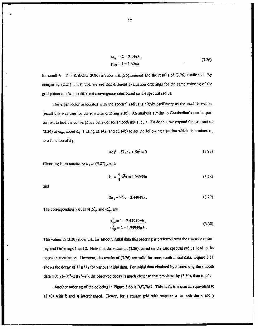
27

apt = 2 - 2.14rth ,(3.26)

Popt I - 1.60th

for small h. This R/B/O/G SOR iteration was programmed and the results of (3.26) confirmed. By

comparing (2.21) and (3.26), we see that different evaluation orderings for the same coloring of the

grid points can lead to different convergence rates based on the spectral radius.

The eigenvector associated with the spectral radius is highly oscillatory as the mesh is r' fined

(recall this was true for the rowwise ordering also). An analysis similar to Garabedian's can be per-

formed to find the convergence behavior for smooth initial data. To do this, we expand the real root of

(3.24) at w, about t=lI using (2.14a) and (2.14b) to get the following equation which determines c1

as a function of k1:

4c, -5kc+662=0 (3.27)

Choosing k 1 to maximize c I in (3.27) yields

I -'l& = 1.95959n (3.28)

and

2c I= 6x = 2.44949nt. (3.29)

The corresponding values of p* and (o, are

p;= 1 - 2.44949th, (3.30)

co = 2 - 1.95959nth.

The values in (3.30) show that for smooth initial data this ordering is preferred over the rowwise order-

ing and Orderings I and 2. Note that the values in (3.26), based on the true spectral radius, lead to the

opposite conclusion. However, the results of (3.26) are valid for nonsmooth initial data. Figure 3.11

shows the decay of I I u 112 for vaiious initial data. For initial data obtained by discretizing the smooth

data u (x ,y)=(x2 -x)(y Z-y), the observed decay is much closer to that predicted by (3.30), than to p'.

Another ordering of the coloring in Figure 3.6b is R/G/B/O. This leads to a quartic equivalent to

(2.10) with 4 and 11 interchanged. Hence, for a square grid with stepsize h in both the x and y

28

directions, w,,, and pp, for this ordering are also given by (2.21). Any of the 24 possible orderings

associated with Figure 3.6b or the 24 orderings of Figure 3.6a can be easily proved (Adams and .or-

danL1986]) to have the same eigenvalues as one of the three orderings (R/B/G/O, R/B/O/G, R/G/B/O)

we have analyzed here. In addition, there is a third coloring of the grid that can be obtained by inter-

changing the rows and columns of Figure 3.6a. Any of the possible 24 orderings of this coloring also

can be proved to be equivalent to one of the three we have analyzed. Hence, the 72 possible four-color

orderings for this model problem can be grouped into two different equivalence classes that character-

ize the asymptotic convergence rate behavior.

I

| I

29

((a)

IO -I - I

0 20 40 60 80 100 120 140 160

i t era ti on

Figure 3.11. Convergence history (2-norm of error versus iteration number) forOrdering #3 with h = 0.05 and ci = 1.66. Three choices of initial data are compared:

(a) An eigenvector corresponding to the spectral radius.(b) An eigenvector corresponding to the largest nonspurious eigenvalue.(c) U = (the - -I)Wic - dt ) m

Note that the realistic initial data (c) more closely matches (b) than (a).

30

4. A nine-point pseudo-SOR method.

We now consider a pseudo SOR method with the stencil in Figure 4. 1,

n n n-I

n+1 n+1 n

Figure 4.1. NR Modified Stencil in Variable n

and iteration

U R + l 1 - ) R o + + 1 Rjk (I) ujk + " (uj7k-1 +Uj-lk+Ujl+ k+l) (4.1)

+ (Uj-k l +Uj- )'2- +Un+lk+1 +Uj+It-I)

which differs from (2.1) in the last two terms. This method can be analyzed using the techniques of

Section 3. The earliest times for two iterations corresponding to Figure 4.1 are equal to those of Figure

3.2. That is, the iteration expressed in terms of the variable v is

u = (1-o) uj - + -21 (Uv-l +UI 'j'k+U7+'k+UjA+1) (4.2)

+ ,j-('+ 1 +u+j-..-I +Uj+lk+l +Uj'*+ik-),

with the change of variables given by (3.3). It is interesting to note that the times in Figure 3.5 and the

iteration in (4.2) are also obtained for a Red/Black ordering of the grid with the Red and Black stencils

shown in Figure 4.2.

• m i I i |1

31

ni n n n+1 n

n n n n n

n+1 n

Red Black

Figure 4.2. Red/Black 9-pt Modified Stencil in Variable n

Since two colors do not decouple a grid discretized with the 9-pt stencil, it is tempting to use old infor-

mation for the Black to Black coupling as shown in Figure 4.2 to obtain a method suitable for parallel

computers. This modification was considered by Kuo, Levy, and Musicus[1986] for a 9-pt stencil aris-

ing from a discretization of a PDE with a cross-derivative term. They show that the convergence rate

of SOR for their problem to be 0 (h) in the region where the lowest frequency dominates. We show

by analyzing (4.2) that the use of only two colors is not sufficient for the 9-pt stencil arising from the

Laplacian. In particular, we will show that the method converges whenever O<co<5/3, that the optimal

omega occurs where the lowest and highest frequencies cross, and that the rate of convergence with

the optimal omega is approximately 37 2h2 for small h as opposed to 1.79nh obtained in Section 3 for

the true SOR method with Orderings #1 or #2.

We begin by observing that ujk=g'sinxjsinrlyk is an eigenmrde of (4.2). We substitute this

into (4.2) to get

g2 =(1 w) +2SO (cos-h+cosih)+- .costhcosrih, (4.3)5 -,

where g 2 is the eigenvalue of the method in (4.1) or the Red/Black method depicted in Figure 4.2. The

eigenvectors in variable n for the NR ordering (4.1) or the Red/Black ordering (Figure 4.2) are the

same as the respective ones given in Section 3 for the 5-point stencil.

Equation (4.3) can be solved for g to get

g = -- (cos th +cosrqh) ± (costh +cosrh)2+(l--w)+ cosho . (4.4)

When w=I, the "pseudo Gauss-Siedel" method has amplification factor

32

2 cosh+cos sh 1s 21 h 12

9± + -i-(cos th 4cosilh ) +(cos.h coshh) (4.5)5 25 5

which is maximized when i=-----. The maximum value is easily determined from (4.5) be cos2ith.

This is identical to the spectral radius of Gauss-Siedel for the model problem with the 5-pt stencil. The

methods, however, differ drastically when (o~l.

To determine the optimal o), we must minimize the maximum modulus of g in (4.4). Two cases

must be considered. First, assume the radical in (4.4) is negative. Then

I g 12 = 0 (1_-L costh cosTih) - 1 (4.6)5

and for convergence, we require I g 12 < I and hence

12-- 1

(4.7)1 - 5 Cos hcosrlh

As h -40, (4.7) shows that the method is divergent for co>5/3. Also (4.6) shows that the value of I g 12

is maximized when cosTh----cos rh. This occurs when l=N- (low frequency in one direction and

high frequency in the other) and this maximum is

Co (+5 cos2nh) - 1. (4.8)

As h--.)0, Ig1,--* 6IC(O- 11.

Secondly, assume the radical in (4.4) is positive. Then, the maximum value of g occurs when

4-T--n and is

2 8 0 2 ~~ 1~= 5 50 cos~ithgm., - coos~nh + (1--) +. -acs2(4.9)

+ -C cos~nh ) 2cos2nh +(l-(o) + .- cos2irh

It is interesting to note that the w that minimizes (4.9) occurs when the radical is zero, and as h -- 0,

w-45/2. That is, the method is divergent for the (o that minimizes g.,,a of (4.9) for the lowest fre-

quency. Recall that the co that is optimal for SOR for consistently ordered matrices corresponds to the

33

lowest frequency. For the pseudo SOR method, the optimal to occurs where the modulus of the eigen-

values of the two frequencies rl=N- k and 71=t-- are equal. This co is determined by equating (4.8)

and (4.9) to get

16o 2cos27rh F.S2coS2 nh+co--I] 4(o&-I)2 = 0. (4.10)25 .5 J

As h -- 0, (o--5/3, so we look for a solution to (4.10) of the form

(h) =-1 + cIh +C2h 2 + "'"(4.11)3

Substituting (4.11) into (4. 10) and equating terms yields

20CI=0, C2=- L

9

and the corresponding values of the optimal wo and spectral radius of (4.1) are

3 9 -(4.12)

Ppw = 1 - 3nh

Comparing (4.12) to cos2rh=l-n 2 h 2, the spectral radius of the pseudo Gauss Siedel method, shows

that as h-0, this method with optimal o is only three times faster than with o--1. This is not nearly as

good as the true SOR methods discussed in Section 3, where the decay factor is 1-0 (h) for the

optimal o.

5. Comparison of point and line methods.

Let the system Ax =b be blocked as

D, -U 12 .. -U I. U I b I

-L 21 D2 . • -U2,, U2 b 2

-L 32 . = . (5.1)

-L. I -L.2 D. _u- b.

34

The line Jacobi method is defined as

Diuj," ILjul + Uju7+b (5.2)j.C<

j>i

and the line-SOR method as

Diu, +' = oLijuin + (o Uju +c i +(1- o) Di., (5.3)/ <i j >i

where ui corresponds to the nodes in row i of the grid. The spectral radius of the Jacobi method for

the 5-pt and 9-pt stencils can easily be found by separation of variables since sin~xisin-qyt is an eigen-

vector of iteration (5.2). These results are given in Figure 5.1.

Method Spectral Radius

5-pt point Cosrnh = 1 -1 7 h 2

5-pt line cosnh 1 - n&h2

2-cosrth

41 2 t~9-pt point Acosnth + -1 cos2rnh = -1

5 5 5

2cosnh + - cos2th

9-pt line = 1 - t2h 2

1 - -1 cosith

Figure 5.1. Spectral Radius of Point and Line Jacobi Methods

The spectral radius of the line-SOR method for the 5-pt and 9-pt stencils can now be found using

Young's theory for block-consistently ordered matrices. That is, if g is the spectral radius of line-

Jacobi then (o, and p,, for line-SOR are given by

2COOpI = 1 + i --2 (5.4)

Popt = (OV - 1.

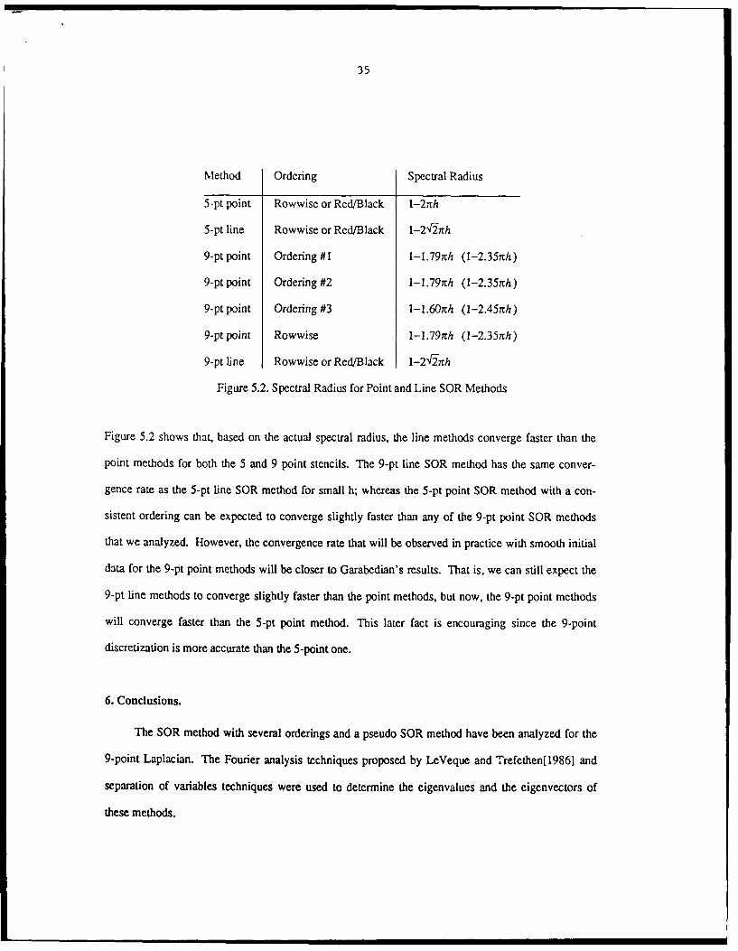
These SOR results are summarized in Figure 5.2 below where Garabedian's results for the 9-pt point

methods are given in parenthesis.

35

Method Ordering Spectral Radius

5-pt point Rowwise or Red/Black 1-27th

5-pt line Rowwise or Red/Black 1-21'2lth

9-pt point Ordering #I I-1.79nth (l-2.35nrh)

9-pt point Ordering #2 1-1.791rh (1-2.35nrh)

9-pt point Ordering #3 1-1.60rnh (1-2.45irh)

9-pt point Rowwise 1-1.797th (1-2.357th)

9-pt line Rowwise or Red/Black 1-2427th

Figure 5.2. Spectral Radius for Point and Line SOR Methods

Figure 5.2 shows that, based on the actual spectral radius, the line methods converge faster than the

point methods for both the 5 and 9 point stencils. The 9-pt line SOR method has the same conver-

gence rate as the 5-pt line SOR method for small h; whereas the 5-pt point SOR method with a con-

sistent ordering can be expected to converge slightly faster than any of the 9-pt point SOR methods

that we analyzed. However, the convergence rate that will be observed in practice with smooth initial

data for the 9-pt point methods will be closer to Garabedian's results. That is, we can still expect the

9-pt line methods to converge slightly faster than the point methods, but now, the 9-pt point methods

will converge faster than the 5-pt point method. This later fact is encouraging since the 9-point

discretization is more accurate than the 5-point one.

6. Conclusions.

The SOR method with several orderings and a pseudo SOR method have been analyzed for the

9-point Laplacian. The Fourier analysis techniques proposed by LeVeque and Trefethen[ 19861 and

separation of variables techniques were used to determine the eigenvalues and the eigenvectors of

these methods.

36

We examined the SOR method for the 9-pt Laplacian using the natural rowwise ordering and

several multicolor orderings. For all these orderings, we gave a quartic equation for the square root of

the eigenvalues as a function of the frequencies and w. The optimal wz was found by solving this quar-

tic numerically for all our orderings. This o) was confirmed for some orderings by asymptotically solv-

ing the quartic corresponding to the lowest frequency for small h. The numerical results indicate that

the lowest frequency determines the convergence rate, but so far we have not proved this.

Our results were confirmed by performing the SOR iteration with an initial guess corresponding

to the eigenvector associated with the spectral radius. The observed rate of convergence matched that

predicted by the theory to five decimal places. The SOR iteration was also performed by using a

smooth initial guess, obtained by discretizing (x-x 2)(y-y 2) for various stepsizes, h. In these cases,

the observed convergence rate more closely resembled that predicted by Garabedian.

The results also show that different orderings of the same coloring can lead to different spectral

radii: R/B/G/O and R/B/O/G for the coloring in 6b have spectral radii of 1-1.79rh and l-1.60"nh

respectively. For smooth initial data, these two orderings also led to different effective spectral radii

observed in practice; namely, 1-2.35nrh and 1-2.45nth, respectively. This information can be useful

in selecting a coloring, an ordering, and appropriate initial data to use with multi-color SOR on parallel

computers (Adams and Ortega[1982).

An analysis of the pseudo SOR method showed that the optimal o occurs when the high and low

frequencies cross and that the corresponding spectral radius is only l-3r12h2. This is inferior to both

the 5-pt and 9-pt SOR methods we analyzed. In addition, for small h, the pseudo method only con-

verges for 0<o)<5/3.

The 5-pt and 9-pt point and line SOR methods were compared for the model problem for small

h. The line methods converge slightly faster than the point methods. The 9-pt line and 5-pt line

methods have the same asymptotic rate of convergence, but the 5-pt point method with a consistent

ordering was 1.12 times faster, based on the spectral radius, and 1.23 times slower, based on

Garabedian's arguments, than the best 9-pt point method that we analyzed. Hence, for a smooth initial

37

guess, the 9-pt point methods can be expected to be more accurate and converge faster than the 5-pt

point method.

Acknowledgemnent

The authors would like to thank Nick Trefethen for providing the initial stimulus for this work

and for several valuable subsequent conversations. We also thank Elizabeth Ong for programming the

SOR method with our orderings.

The authors wish to dedicate this paper, as a token of their highest esteem, to Professor Werner

Rheinboldt on the occasion of his sixtieth birthday.

References

Adams, L.M., Ortega, J.M. (1982]. "A Multi-Color SOR Method for Parallel Computation,"Proc. of the 1982 Intl. Conference on Parallel Processing, IEEE Catalog No, 82CH1794-7,August, pp. 53-56.

Adams, Loyce M., Jordan, Harry F. (19861. "Is SOR Color-blind?", Siam Journal on Scientificand Statistical Computing, Vol. 7, No. 2, April, pp. 490-506.

Forsythe, G., Wasow, W. [1960]. Finite-Difference Methods For Partial Differential Equations,John Wiley & Sons, Inc., New York, pp. 266.

Frankel, S. (950]. "Convergence Rates of Iterative Treatments of Partial Differential Equations,"Math. Comp. 4, pp. 65-75.

Garabedian, P. (19561. "Estimation of the Relaxation Factor for Small Mesh Size," Math. Comp.10, pp. 183-185.

Kuo C., Levy B., Musicus B. [19861. "A Local Relaxation Method for Solving Elliptic PDEs onMesh-Connected Arrays," submitted to Siam Journal on Scientific and Statistical Comput-ing.

LeVeque R. and Trefethen L.N. [1986]. "Fourier Analysis of the SOR Iteration," submitted toSIAM Journal of Numerical Analysis.

38

Young, David M. [1950]. "Iterative Methods for Solving Partial Differential Equations of EllipticType," Doctoral thesis, Harvard University, Cambridge, Mass.

Young, David M. [19711. Iterative Solution of Large Linear Systems, Academic Press, NewYork.

Standard Bibliographic Page

1. Report No. NASA CR- 178212 vernment Accession No. 3. Recipient's Catalog No.ICASE Report No. 86-81

4. Title sand Subtitle 5. Report Date

ANALYSIS OF THE SOR ITERATION FOR THE 9-POINT December 1986

LAPLACIAN 6. Performing Organization Code

7. Author(s) 8. Performing Organization Report No.

Loyce Adams, Randy LeVeque, David Young 86-81

9. Perfo ing Orgiaizatien Name and in ceddrn 10. Work Unit No.Inst tute or omputer Ipp cations in Scienceand Engineering 11. ContractIg8Gnt No.

Mail Stop 132C, NASA Langley Research Center NAS- 1 ntoHampton, VA 23665-5225Hampon, A2365-52513. Type of Report and Period Covered

12. Sponsoring Agency Name and Address

Contractor ReportNational Aeronautics and Space Administration 14. Sponsoring Agency Code

Washington, D.C. 20546 50-9-2 l-Cf

15. Supplementary Notes

Langley Technical Monitor: Submitted to SIAM Journal onJ. C. South Numerical Analysis

Final Report16. Abstract

The SOR iteration for solving linear systems of equations depends upon anoverrelaxation factor W . A theory for determining W was given by Young[1950] for consistently ordered matrices. Here we determine the optimal Wfor the 9-point stencil for the model problem of Laplace's equation on asquare. We consider several orderings of the equations, including the naturalrowwise and multicolor orderings, all of which lead to non-consistently orderedmatrices, and find two equivalence classes of orderings with differentconvergerce behavior and optimal w's. We compare our results for the naturalrowwise ordering to those of Garabedian [1956] and explain why both results are,in a sense, correct, even though they differ. We also analyze a pseudo SORmethod for the model problem and show that it is not as effective as the SORmethods. Finally, we compare the point SOR methods to known results for lineSOR methods for this problem.

17. Key Words (Suggested by Authors(s)) 18. Distribution Statement

SOR (successive overrelaxation), 64 - Numerical Analysismulticolor orderings

Unclassified - unlimited19. Security Clasif.(of this report) 20. Security Classif.(of this page) 21. No. of Pages 22. Price

Unclassified Unclassified 40 A03

For sale by the National Technical Information Service, Springfield, Virginia 22161

NASA-Langley, 1987