sound source ion using labview
TRANSCRIPT
R.V. COLLEGE OF ENGINEERING, Bangalore-560059
(Autonomous Institution Affiliated to VTU, Belgaum)
“SOUND SOURCE LOCALIZATION USING
LabVIEW”
PROJECT REPORT2011-12
Submitted by
1. JAGRITI R 1RV08IT058
2. SHREE VARDHAN SARAF 1RV08IT061
Under the Guidance of
Mr. HARSHA HERLE Assistant professor
Department of Instrumentation Technology, RVCE
In partial fulfillment for the award of degree
of
Bachelor of Engineering
in
INSTRUMENTATION TECHNOLOGY

R.V. COLLEGE OF ENGINEERING, BANGALORE – 560059(Autonomous Institution Affiliated to VTU, Belgaum)
DEPARTMENT OF INSTRUMENTATION TECHNOLOGY
CERTIFICATE
Certified that the project work titled ‘Sound source localization using LabVIEW’ is
carried out by Jagriti R (1RV08IT058) and Shree Vardhan (1RV08IT061) who are
bonafide students of R.V College of Engineering, Bangalore, in partial fulfillment for
the award of degree of Bachelor of Engineering in Instrumentation Technology of
the Visvesvaraya Technological University, Belgaum during the year 2011-2012. It is
certified that all corrections/suggestions indicated for the internal Assessment have
been incorporated in the report deposited in the departmental library. The project
report has been approved as it satisfies the academic requirements in respect of
project work prescribed by the institution for the said degree.
Signature of Guide: Signature of Head of Department: Signature of Principal
External Viva
Name of Examiners Signature with date
1
2
R.VCOLLEGE OF ENGINEERING, BANGALORE - 560059(Autonomous Institution Affiliated to VTU, Belgaum)
DEPARTMENT OF INSTRUMENTATION TECHNOLOGY
DECLARATION
We, Jagriti R (1RV08IT058) and Shree Vardhan Saraf (1RV08IT061) the
students of eighth semester B.E., Instrumentation Technology, hereby declare that
the project titled “Sound source localization using LabVIEW” has been carried out
by us and submitted in partial fulfillment for the award of degree of Bachelor of
Engineering in Instrumentation Technology. We do declare that this work is not
carried out by any other students for the award of degree in any other branch.
Place: Bangalore Names Signature
Date: 1. Jagriti R
2. Shree Vardhan
ACKNOWLEDGEMENT
The satisfaction that accompanies the successful completion of any endeavour would
be incomplete without the mention of people who made it possible and whose
constant support, encouragement and guidance has been a source of inspiration
throughout the course of this project.
We thank our internal guide Mr. Harsha Herle, Assistant Professor, Instrumentation
Technology, R.V College of Engineering for his endearing help and guidance.
We express our heart-felt gratitude to Mr. Rohit Pannikar, Manager, Applications
engineering division and Mr. Rajshekhar, Staff Applications engineer, National
Instruments India for providing a very congenial work environment and for their
expert supervision that enabled us to complete this project successfully in the given
duration.
We would like to thank Dr. Prasanna Kumar S.C., Professor and Head of
Department of Instrumentation Technology, R.V College of Engineering, Bangalore
for his encouragement and support.
We would like to thank Prof. B.S. Satyanarayana, Principal, R.V College of
Engineering for his constant support.
Finally, we thank one and all involved directly or indirectly in successful completion
of the project.

ABSTRACT
Problem of locating a sound source in space has received a growing interest. The
human auditory system uses several cues for sound source localization, including
time- and level-differences between ears, spectral information, timing analysis,
correlation analysis, and pattern matching. Similarly, a biologically inspired sound
localization system can be built by making use of an array of microphones, which are
hooked up to a computer.
Methods for determining the direction of incidence based on sound intensity, the
phase of cross-spectral functions, cross-correlation functions, and Frequency
Selection algorithm are available. Sound source localizations finds applications in
military, camera pointing in video-conferencing environments, beam former steering
for robust speech recognition systems etc.
There is no universal solution for accurate sound source localization. Depending on
the object under study and the noise problem, the most appropriate technique has to
be selected. In this project we attempt to localize a single sound source by using four
microphones. A most practical acoustic source localization scheme is based on time
delay of arrival estimation (TDOA). We implement generalized cross correlation to
find time delay of arrival between microphone pairs. TDOA estimation using
microphone arrays is to use the phase information present in signals from
microphones that are spatially separated. Phase difference between the Fourier
transformed signals to estimate the TDOA and is implemented using a 4 element
tetrahedron shaped microphone array.
Once TDOA estimation is performed, it is possible to find the position of the source
through geometrical calculations therefore deriving the source location by solving the
set of non-linear least squares equations. The experimental results showed that the
direction of the two sources was estimated with high accuracy while the range of the
sources was estimated with moderate accuracy.
\i
CONTENTS
Abstract iList of Figures iiList of Tables iii List of symbols, Acronyms and Nomenclature i
1. Chapter 1: Introduction 1 1.1 Sound localization in Biology 2 1.2 Sound localization: a signal processing view 31.3 Problem statement 41.4 Objective 41.5 Overview of the Project 5 1.6 Organization of Report 51.7 Block Diagram and Description 6
2. Chapter 2: Theoretical Background 72.1 Nature of Sound 82.2 Microphone 10
2.2.1 Types of microphone 112.3 Microphone array 132.4 Various Coherence Measures 14
3. Chapter 3: Design and methodology 153.1 Scenario 163.2 Direction of Arrival Estimation 16
3.2.1 The Geometry of the Problem 163.2.2 Microphone array structure 173.2.3 Time Delay of Arrival (TDOA) 183.2.4 Algorithm to find Time delay of Arrival 19
3.3 Distance Estimation 213.3.1 Source Localization in 2-Dimensional Space 213.3.2 Hyperbolic position location 21
3.3.2.1 General Model 223.3.2.2 Position Estimation 23
3.4 Hardware Design 243.4.1 cDAQ-9172 243.4.2 Analog input module - NI 9234 243.4.3 Digital output module – NI 9472 24

3.5 Assumptions and Limitations 25
4. Chapter 4: Implementation Overview 26 4.1 Hardware and interfacing 274.2 Overview of LabVIEW 27
4.2.1 Front panel 284.2.2 Block diagram 28
4.3 Programming using LabVIEW 11 294.3.1 Microphone signal interface using NI DAQ Assistant. 294.3.2 Threshold detection of each signal 324.3.3 Finding time delay of arrival 344.3.4 Direction and distance estimation 364.3.5 Servo control 37
4.4 System Hardware 374.4.1 Microphone 384.4.2 The microphone array 384.4.3 Data Acquisition 39
4.4.3.1 Modules 404.5 Flow Chart 42
5. Chapter 5: Results and Discussion 435.1 Experimental Setup 445.2 Experiment 1: Time delay of arrival 455.3 Experiment 2: Direction of arrival 465.4 Experiment 3: Distance estimation 47
6. Chapter 6: Conclusion and future work 496.1 Conclusion 506.2 Future work 50
7. Chapter 6: Appendix 527.1 Bibliography 537.2 Snapshots of working model 557.3 Datasheets 57
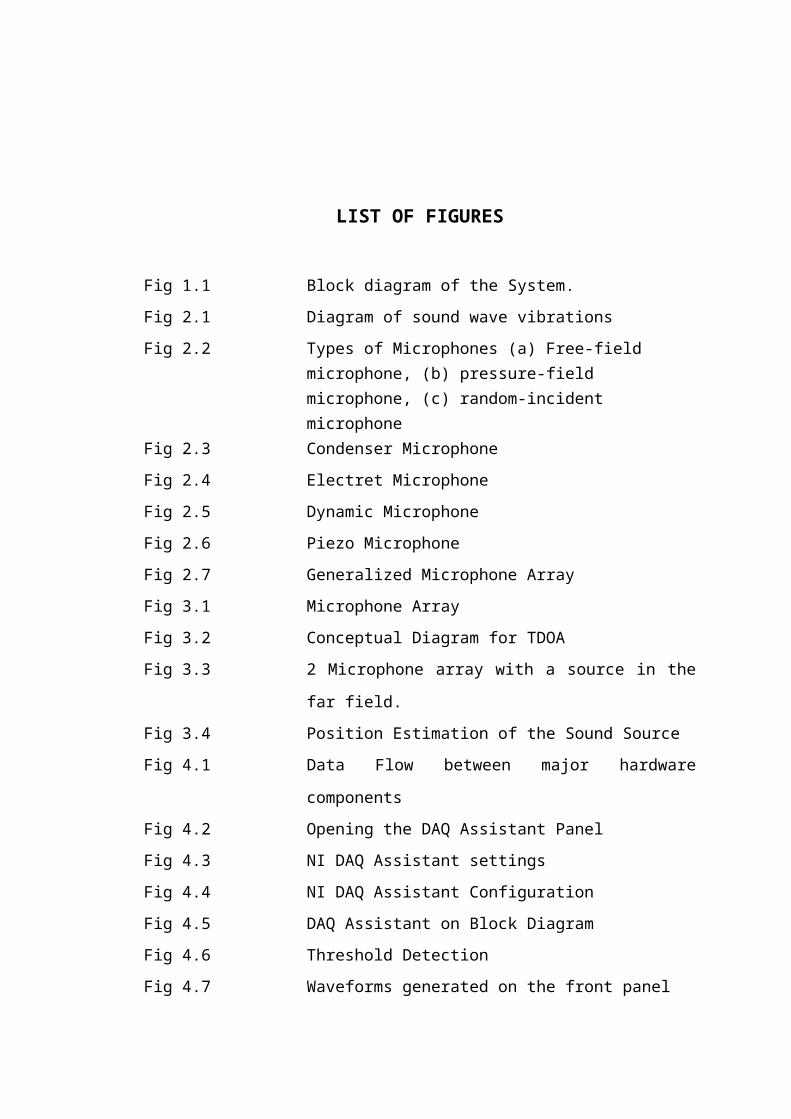
LIST OF FIGURES
Fig 1.1 Block diagram of the System.
Fig 2.1 Diagram of sound wave vibrations
Fig 2.2 Types of Microphones (a) Free-field microphone, (b) pressure-field microphone, (c) random-incident microphone
Fig 2.3 Condenser Microphone
Fig 2.4 Electret Microphone
Fig 2.5 Dynamic Microphone
Fig 2.6 Piezo Microphone
Fig 2.7 Generalized Microphone Array
Fig 3.1 Microphone Array
Fig 3.2 Conceptual Diagram for TDOA
Fig 3.3 2 Microphone array with a source in the far field.
Fig 3.4 Position Estimation of the Sound Source
Fig 4.1 Data Flow between major hardware components
Fig 4.2 Opening the DAQ Assistant Panel
Fig 4.3 NI DAQ Assistant settings
Fig 4.4 NI DAQ Assistant Configuration
Fig 4.5 DAQ Assistant on Block Diagram
Fig 4.6 Threshold Detection
Fig 4.7 Waveforms generated on the front panel
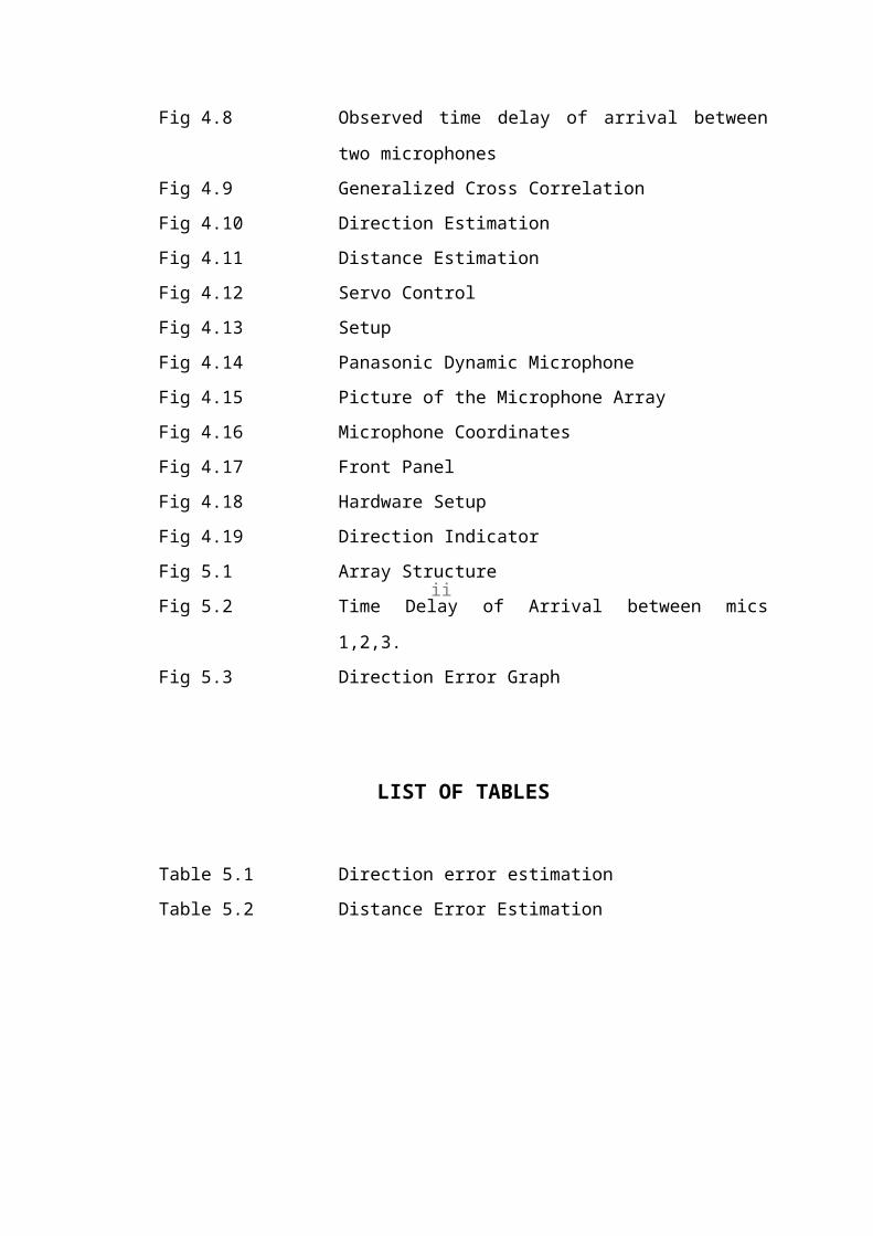
Fig 4.8 Observed time delay of arrival between two microphones
Fig 4.9 Generalized Cross Correlation
Fig 4.10 Direction Estimation
Fig 4.11 Distance Estimation
Fig 4.12 Servo Control
Fig 4.13 Setup
Fig 4.14 Panasonic Dynamic Microphone
Fig 4.15 Picture of the Microphone Array
Fig 4.16 Microphone Coordinates
Fig 4.17 Front Panel
Fig 4.18 Hardware Setup
Fig 4.19 Direction Indicator
Fig 5.1 Array Structure
Fig 5.2 Time Delay of Arrival between mics 1,2,3.
Fig 5.3 Direction Error Graph
LIST OF TABLES
Table 5.1 Direction error estimation
Table 5.2 Distance Error Estimation
ii
iii
List of symbols, Abbreviations and Nomenclature
DOA – Direction of Arrival
GCC - Generalized Cross Correlation
GCCPHAT - GCC Phase Transform
SSL – Sound source localization
TDE - Time Delay Estimation
TDOA - Time Difference Of Arrival
PL - Position Location
2-D - Two dimensional
3-D - Three dimensional
DFT- Discrete Fourier Transform
FFT - Fast Fourier Transform
iv
R V College of Engineering
CHAPTER – 1
INTRODUCTION
Department of Instrumentation Technology Page 1
R V College of Engineering
Chapter 1
INTRODUCTION
1.1 Sound localization in Biology
For many species such as barn owl, sound localization is a matter of survival. The
natural capabilities of human and animals to localize sound has intrigued researchers
for many years. Numerous studies have attempted to determine the processes and
mechanisms used by humans or animals to achieve spatial hearing.
One of the first steps in understanding nature's way of solving this problem is to
understand how information is processed in the ear. A number of models for the ear
have been suggested by the researchers [11]. These studies suggest that the cochlea
effectively extracts the spectral information from the sound wave impinging on the
ear drums and converts it into the electrical signals. The cochlear output is in the form
of electrical signals at different neuron points along the basilar memebrane of cochlea.
The electrical signals then travel up to the brain for further processing.
Many researchers have come up with different models of processing of electrical
signals in the brain for sound localization to support the experimental data from
various neurophysiological studies. All these different models agree on the
fundamental view that the direction of the sound is determined by two important
binaural cues - the interaural time difference and the interaural level difference. These
binaural cues arise from the differences in the sound waveforms entering the two ears.
The interaural time difference is the temporal difference in the waveforms due to the
delay in reaching the ear farther away from the sound source. The interaural level
difference is the difference in the intensity of the sound reaching the two ears. In
general, the ear which is farther away from the source will receive a fainter sound
than the ear which is relatively closer to the source due to the attenuation effect of the
head and surroundings. The phenomena of time delay and the intensity difference can
be integrated into the notion of interaural transfer function which represents the
transfer function between the two ears.
Department of Instrumentation Technology Page 2
R V College of Engineering
In general, the task that the human auditory system performs in order to detect,
localize, recognize and emphasize different sound sources is referred to as auditory
scene analysis (ASA). An auditory scene denotes the listener and his/her physical
surroundings, including sound sources.
It is generally accepted that cross-correlation based computational models for binaural
processing provide excellent qualitative and quantitative accounts of experimental
studies. The output patterns obtained from the cross-correlation operations reflect the
binaural information which can be refined further and interpreted to determine the
direction of the source.
1.2 Sound localization: a signal processing view
In the signal processing community, the more commonly used term for this problem is
direction-of-arrival (DOA) estimation
Time Delay Estimation between replicas of signals is intrinsic to many signal
processing applications. Depending on the type of signals acquired ranging from
human hearing to radars, various Time Delay Estimation methods have been
described in literature [9]. Sound source localization (SSL) systems estimate the
location of audio sources based on signals received by an array of microphones. With
proper microphone geometry, SSL systems can also provide 3D location information.
The other example of SSL is to locate sound sources so that a robot can interact with
detected objects. Rotating a microphone in a conference room to isolate and process a
particular speaker is another example where SSL systems can be implemented.
In general, there are three categories of techniques for sound source localization, i.e.
steered-beamformer based, high resolution spectral estimation based, and time delay
of arrival (TDOA) based [10].
The direction of the sound source can be obtained by estimating the relative Time
Delay of Arrival (TDOA) between two microphones. Peak levels for each microphone
signal are analyzed, from which a time delay between signals can be found. The
location of the source relative to the microphone array is calculated using this delay,
and this location is displayed on the computer screen.
Department of Instrumentation Technology Page 3
R V College of Engineering
1.3 Problem statement
Sound Source Localization system is to determine the location of audio sources based
on the audio signals received by an array of microphones at different positions in the
environment.
Sound source localization is a complex and cumbersome task. The toughest challenge
facing any acoustics engineer is to figure out where the sound originates – especially
when there is considerable interference and reverberation flying around.
Even though a number of basic techniques exist and have undergone constant
improvement, the problem remains that there is no “magical” sound source
localization technique that prevails over the others. Depending on the test object, the
nature of the sound and the actual environment, engineers have to select one method
or the other [8].
1.4 Objective
In this Project we have studied the available techniques and eventually developed an
algorithm as we attempt to localize a sound source. Using an array of 5 microphones,
the direction of the sound source as well as well as the distance to the sound source is
estimated.
The first step computes TDOA for each microphone pair, and the second step
combines these estimates using a set of equations to obtain the direction vector and
distance coordinates.
Department of Instrumentation Technology Page 4
R V College of Engineering
1.5Overview of the Project
The procedure for localization of multiple sound sources by the TDOA method is:
1. Estimation of delays of arrival[2]
2. Localization by clustering delay of arrivals[3]
3. Display the sound location.
A simple method of localization is to estimate the time delay of arrival (TDOA) of a
sound signal between the two microphones. This TDOA estimate is then used to
calculate the Angle of Arrival (AoA). The most commonly used TDOA estimation
method is generalized cross correlation (GCC). The TDOA estimate τ can be
calculated by applying the cross correlation equation. The sample corresponding to
the maximum coefficient denotes the time delay in number of samples.
Combining the data from two microphone pairs and by using the process of
hyperbolic position estimation, we compute the distance of sound source from the
microphone pairs
A microphone cluster was set up in a lab with coordinates, where
the microphones were placed at the corners of a known array. A
sound localization experiment was done whose results proved the
measured success of the sound localization routine implemented in
LabVIEW.
1.6 Organization of Report
Chapter 1 introduces a brief literature along with the latest
application of the project. The block diagram explains the working.
Chapter 2 deals with the theory behind the nature of sound and the
acquisition of the same using different types of microphones.
Chapter 3 describes the methodology along with the algorithms
used. Chapter 4 explains the system software and hardware
implementation. In Chapter 5, the readings have been tabulated
Department of Instrumentation Technology Page 5
R V College of Engineering
and the discrepancies are discussed. Chapter 6 concludes the work
and the future scope of the project is discussed. Finally the
snapshots of the working model along with the datasheets are
presented in chapter 7.
1.7 Block Diagram and Description
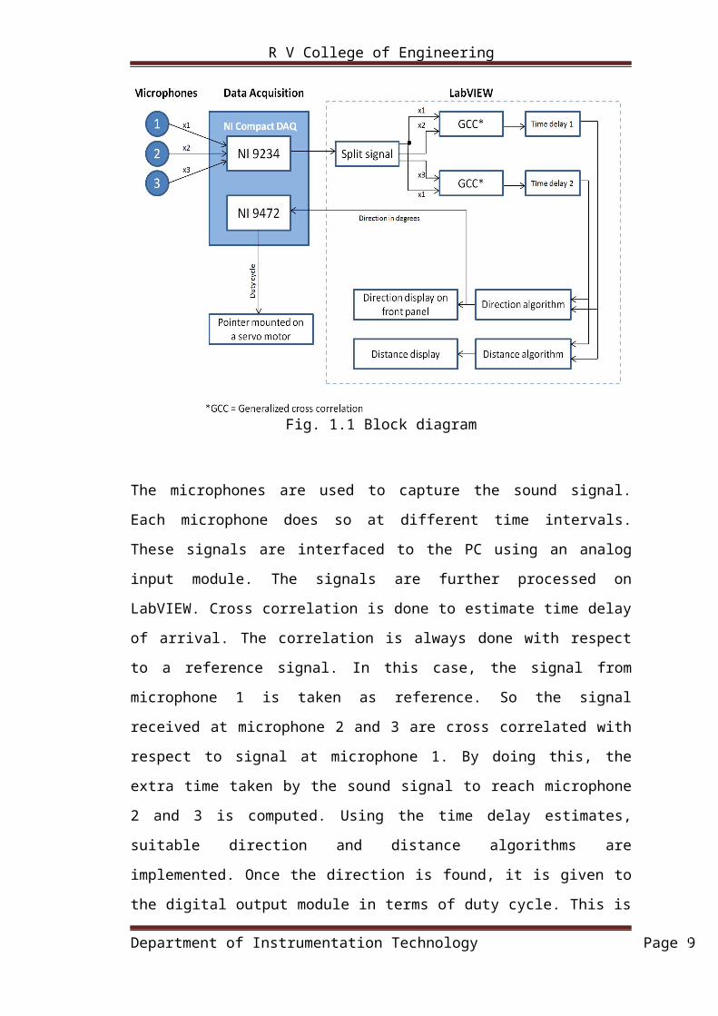
A simplified block diagram showing the process involved using three microphones is
shown below in Fig 1.1.
Fig. 1.1 Block diagram
The microphones are used to capture the sound signal. Each microphone does so at
different time intervals. These signals are interfaced to the PC using an analog input
module. The signals are further processed on LabVIEW. Cross correlation is done to
estimate time delay of arrival. The correlation is always done with respect to a
reference signal. In this case, the signal from microphone 1 is taken as reference. So
the signal received at microphone 2 and 3 are cross correlated with respect to signal at
microphone 1. By doing this, the extra time taken by the sound signal to reach
microphone 2 and 3 is computed. Using the time delay estimates, suitable direction
and distance algorithms are implemented. Once the direction is found, it is given to
the digital output module in terms of duty cycle. This is used to drive a servo motor
Department of Instrumentation Technology Page 6
R V College of Engineering
which houses a pointer. So by doing this, the direction and distance are indicated on
the front panel as well as a visual indication of the direction of sound source. In the
following chapter each of the blocks are explained in detail.
Chapter – 2
THEORETICAL BACKGROUND
Department of Instrumentation Technology Page 7
R V College of Engineering
Chapter 2
THEORETICAL BACKGROUND
Many audio processing applications can obtain substantial benefits from the
knowledge of the spatial position of the source which is emitting the signal under
process. For this reason many efforts have been devoted to investigating this research
area and several alternative approaches have been proposed over the years. [1]
Microphone arrays have been implemented in many applications, including
teleconferencing, speech recognition, and position location of dominant speaker in an
auditorium. Direction of arrival estimation of acoustic signals using a set of spatially
separated microphones has many practical applications in everyday life. DOA
estimates from the set of microphones can be used to automatically steer cameras to
the speaker in a conference room.
Techniques such as the generalized cross correlation (GCC) method, phase transform
(GCC-PHAT) are widely used for DOA estimation [9].
Accuracy of the system depends on various factors. The hardware used for data
acquisition, sampling frequency, number of microphones used for data acquisition,
and noise present in the signals captured, determine the accuracy of the estimates.
Increase in the number of microphones increases the performance of source location
estimation.
2.1 Nature of Sound
Sound is a variation in the pressure of the air of a type which has an effect on our ears
and brain. These pressure variations transfer energy from a source of vibration that
can be naturally-occurring, such as by the wind or produced by humans such as by
Department of Instrumentation Technology Page 8
R V College of Engineering
speech. Sound in the air can be caused by a variety of vibrations, such as the
following.
Moving objects: examples include loudspeakers, guitar strings, vibrating walls
and human vocal chords.
Moving air: examples include horns, organ pipes, mechanical fans and jet
engines.
A vibrating object compresses adjacent particles of air as it moves in one direction
and leaves the particles of air ‘spread out’ as it moves in the other direction. The
displaced particles pass on their extra energy and a pattern of compressions and
rarefactions travels out from the source, while the individual particles return to their
original positions.
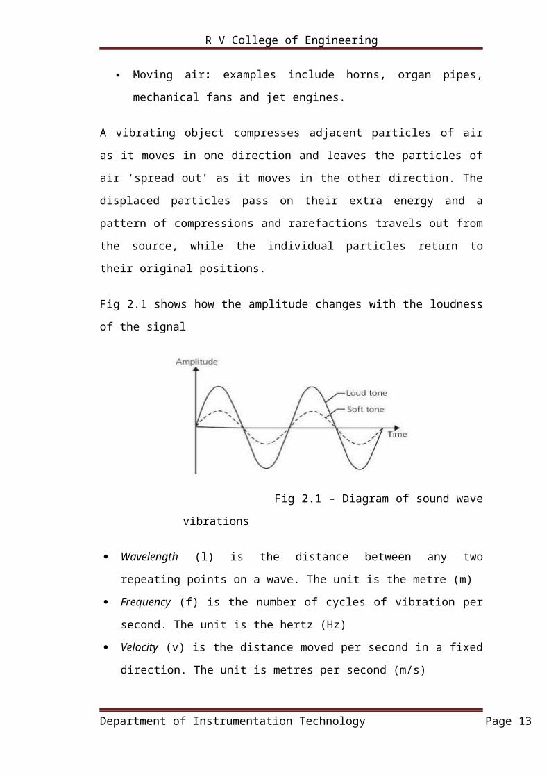
Fig 2.1 shows how the amplitude changes with the loudness of the signal
Fig 2.1 – Diagram of sound wave vibrations
Wavelength (l) is the distance between any two repeating points on a wave. The
unit is the metre (m)
Frequency (f) is the number of cycles of vibration per second. The unit is the
hertz (Hz)
Velocity (v) is the distance moved per second in a fixed direction. The unit is
metres per second (m/s)
For every vibration of the sound source the wave moves forward by one wavelength.
The length of one wavelength multiplied by the number of vibrations per second
therefore gives the total length the wave motion moves in 1 second. This total length
Department of Instrumentation Technology Page 9
R V College of Engineering
per second is also the velocity. This relationship between velocity, frequency and
wavelength is true for all wave motions. A sound wave travels away from its source
with a speed of 344 m/s (770 miles per hour) when measured in dry air at 20 °C (68
°F) . If an object that produces sound waves vibrates 100 times a second, for example,
then the frequency of that sound wave will be 100 Hz.
2.2 Microphone
A microphone is an acoustic-to-electric transducer or sensor that converts sound into
an electrical signal. Most microphones today use electromagnetic induction (dynamic
microphone), capacitance change (condenser microphone), piezoelectric generation,
or light modulation to produce an electrical voltage signal from mechanical vibration.
They can be classified depending on the type of field: free-field, pressure-field, and
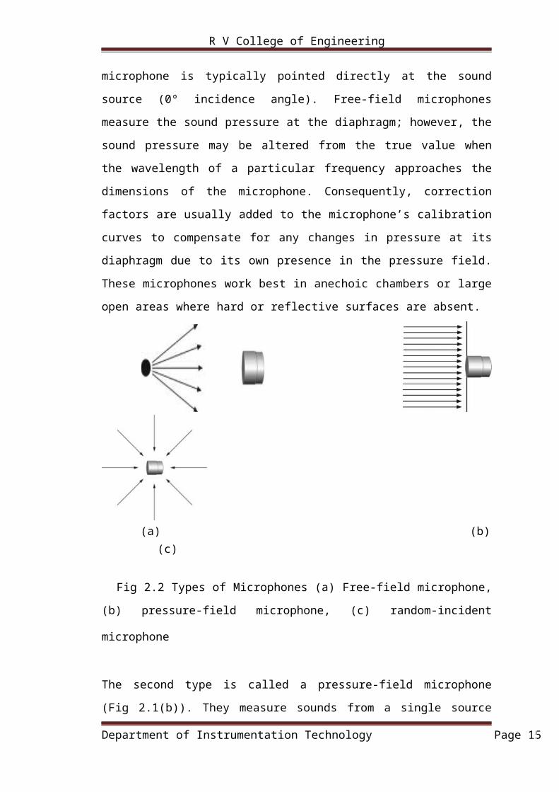
random-incident (diffuse) field. As shown in Fig 2.1(a), Free-field microphones are
intended for measuring sound pressure variations that radiate freely through a
continuous medium, such as air, from a single source without any interference. The
microphone is typically pointed directly at the sound source (0º incidence angle).
Free-field microphones measure the sound pressure at the diaphragm; however, the
sound pressure may be altered from the true value when the wavelength of a particular
frequency approaches the dimensions of the microphone. Consequently, correction
factors are usually added to the microphone’s calibration curves to compensate for
any changes in pressure at its diaphragm due to its own presence in the pressure field.
These microphones work best in anechoic chambers or large open areas where hard or
reflective surfaces are absent.
(a) (b) (c)
Fig 2.2 Types of Microphones (a) Free-field microphone, (b) pressure-field
microphone, (c) random-incident microphone
Department of Instrumentation Technology Page 10
R V College of Engineering
The second type is called a pressure-field microphone (Fig 2.1(b)). They measure
sounds from a single source within a pressure field that has the same magnitude and
phase at any location. In order to simulate a uniform pressure field, they are usually
calibrated in enclosures or cavities, which are small compared to their wavelength.
This minimizes any alterations in measurements due to the presence of the
microphone in the sound field. They are also supplied with a pressure versus
frequency-response curve. Such microphones measure the pressure exerted on walls,
airplane wings, or inside structures such as tubes, housings, and cavities.
The third type is called a random-incident or a diffuse-field microphone. Shown in
Fig 2.11(c) they are omni-directional and measure sound pressure from multiple
directions and sources, including reflections. They come with typical frequency
response curves for different angles of incidence and compensate for the effect of
their own presence in the field. An appropriate application for this type of microphone
is measuring sound in a building with hard, reflective walls, such as a church.
2.2.1 Types of microphone
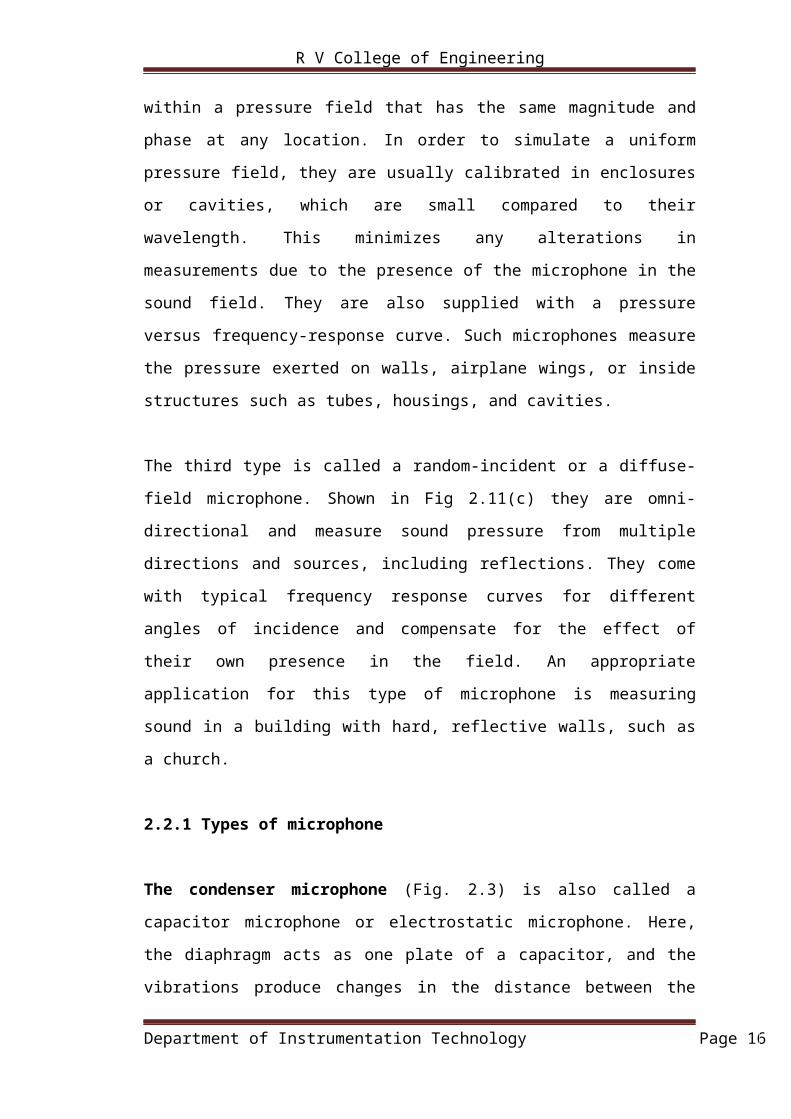
The condenser microphone (Fig. 2.3) is also called a capacitor microphone or
electrostatic microphone. Here, the diaphragm acts as one plate of a capacitor, and the
vibrations produce changes in the distance between the plates. Condenser
microphones span the range from telephone transmitters through inexpensive karaoke
microphones to high-fidelity recording microphones.
Fig. 2.3 Condenser microphone
Department of Instrumentation Technology Page 11
R V College of Engineering
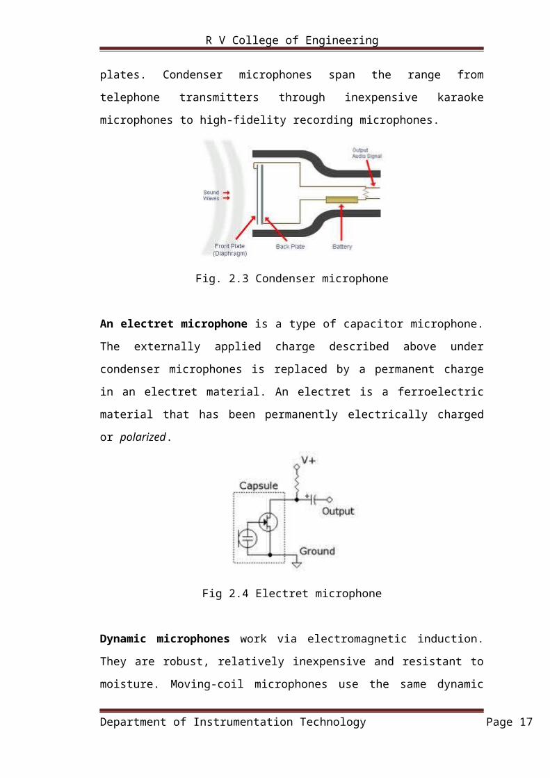
An electret microphone is a type of capacitor microphone. The externally applied
charge described above under condenser microphones is replaced by a permanent
charge in an electret material. An electret is a ferroelectric material that has been
permanently electrically charged or polarized.
Fig 2.4 Electret microphone
Dynamic microphones work via electromagnetic induction. They are robust,
relatively inexpensive and resistant to moisture. Moving-coil microphones use the
same dynamic principle as in a loudspeaker, only reversed. A small movable
induction coil, positioned in the magnetic field of a permanent magnet, is attached to
the diaphragm. When sound enters through the windscreen of the microphone, the
sound wave moves the diaphragm. When the diaphragm vibrates, the coil moves in
the magnetic field, producing a varying current in the coil through electromagnetic
induction
Fig. 2.5 Dynamic microphone
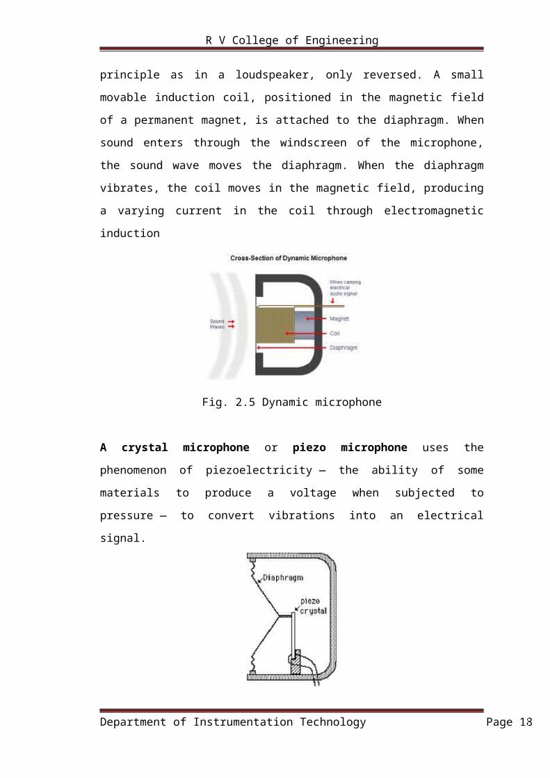
A crystal microphone or piezo microphone uses the phenomenon of
piezoelectricity — the ability of some materials to produce a voltage when subjected
to pressure — to convert vibrations into an electrical signal.
Department of Instrumentation Technology Page 12
R V College of Engineering
Fig 2.6 Piezo microphone
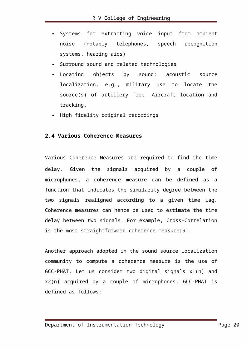
2.3 Microphone array
A microphone array is any number of microphones operating in tandem.
Microphone arrays consist of multiple microphones functioning as a single directional
input device: essentially, an acoustic antenna. Using sound propagation principles, the
principal sound sources in an environment can be spatially located and distinguished
from each other. Distinguishing sounds based on the spatial location of their source is
achieved by filtering and combining the individual microphone signals. The location
of the principal sounds sources may be determined dynamically by analyzing peaks in
the correlation function between different microphone channels.
Fig 2.7 Microphone array
There are many applications:
Systems for extracting voice input from ambient noise (notably telephones,
speech recognition systems, hearing aids)
Surround sound and related technologies
Department of Instrumentation Technology Page 13
R V College of Engineering
Locating objects by sound: acoustic source localization, e.g., military use to
locate the source(s) of artillery fire. Aircraft location and tracking.
High fidelity original recordings
2.4 Various Coherence Measures
Various Coherence Measures are required to find the time delay. Given the signals
acquired by a couple of microphones, a coherence measure can be defined as a
function that indicates the similarity degree between the two signals realigned
according to a given time lag. Coherence measures can hence be used to estimate the
time delay between two signals. For example, Cross-Correlation is the most
straightforward coherence measure[9].
Another approach adopted in the sound source localization community to compute a
coherence measure is the use of GCC-PHAT. Let us consider two digital signals x1(n)
and x2(n) acquired by a couple of microphones, GCC-PHAT is defined as follows:
GCC-PHAT (d) = IFFT X1 · X2*
|X1||X2|
where d is a time lag, subject to |d| < _max, while X1 and X2 are the DFT transforms
of x1 and x2 respectively. The inter-microphone distance determines the maximum
valid time delay _max. It has been shown that, in ideal conditions, GCC-PHAT
presents a prominent peak in correspondence of the actual TDOA. On the other hand,
reverberation introduces spurious peaks which may lead to wrong TDOA estimates
An alternative way to obtain a coherence measure is offered by AED that is able to
provide a rough estimation of the impulse responses that describe the wave
propagation from one acoustic source to two microphones. Under the assumption that
the main peak of each impulse response identifies the direct path between the source
and the microphone, the TDOA can be estimated as the time difference between the
two main peaks. Let us denote with h1 and h2 the two impulse responses, in ideal
conditions, i.e. without noise, the following equation holds:
h2 *x1(n) = h2 *h1 *s(n) = h1 *x2(n)
Department of Instrumentation Technology Page 14
R V College of Engineering
Chapter – 3
DESIGN AND METHODOLOGY
Department of Instrumentation Technology Page 15
R V College of Engineering
Chapter - 3
DESIGN AND METHODOLOGY
1.8 Scenario
Given a set of M acoustic sensors (microphones) in known locations, our goal is to
estimate two or three dimensional coordinates of the acoustic sound source. We
assume that source is present in a defined coordinate system. We know the number of
sensors present and that single sound source is present in the system. The sound
source is excited using a broad band signal with defined bandwidth and the signal is
captured by each of the acoustic sensors. The TDOA is estimated from the captured
audio signals. The TDOA for a given pair of microphones and speaker is defined as
the difference in the time taken by the acoustic signal to travel from the speaker to the
microphones. We assume that the signal emitted from the speaker does not interfere
with the noise sources. Computation of the time delay between signals from any pair
of microphones can be performed by first computing the cross- correlation function of
the two signals. The lag at which the cross-correlation function has its maximum is
taken as the time delay between the two signals.
3.2 Direction of Arrival Estimation
3.2.1 The Geometry of the Problem
Analyzing the geometry of the problem is important; because it
allows us to address the following issues. Any source localization
system can be prone to bewilderment regarding the location of the
source due to aliases. Aliases arise when we do not have enough
sensors or when the geometric placement of the sensors makes
some of them redundant. The problem of aliases can be solved by
adding more sensors to our localization system. However,
consideration of the geometry of the problem allows us to add
microphones economically. That is, we can determine the minimum
number of microphones needed for any given situation. In some
Department of Instrumentation Technology Page 16
R V College of Engineering
cases, we may need to constrain the degree of freedom of the
source of sound. This allows us to do simple experiments by using
even smaller number of microphones than the number of
microphones that we would need to localize a source in 3D. It is
evident that no source localization can be achieved using one
microphone. So, we start by looking at how we need to constrain our
source of sound, assuming that we only have two microphones. The
only way that a source can be localized to a point using two
microphones is if the source is constrained to a line that passes
through the two microphones. If this constraint is lifted, the
precision of the system degrades. We consider adding a third
microphone to our system because we want to ameliorate the
constraints placed on the source. Such constraints were imposed to
make the system precise to a point. Adding a third microphone on a
line that passes through the previous two microphones results in
redundancy. Thus, the three microphones should not all be on a
single line. Three microphones placed at the corners of a triangle
may seem to be adequate to localize a source to a point in a plane.
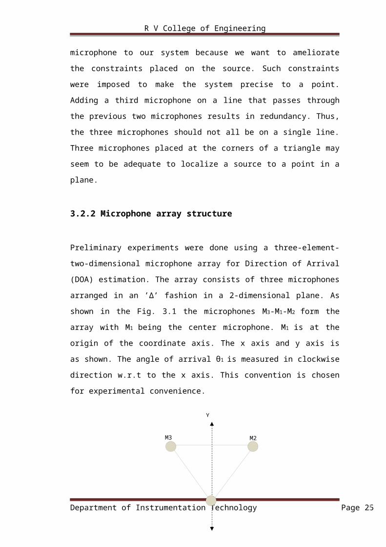
3.2.2 Microphone array structure
Preliminary experiments were done using a three-element-two-dimensional
microphone array for Direction of Arrival (DOA) estimation. The array consists of
three microphones arranged in an ’Δ’ fashion in a 2-dimensional plane. As shown in
the Fig. 3.1 the microphones M3-M1-M2 form the array with M1 being the center
microphone. M1 is at the origin of the coordinate axis. The x axis and y axis is as
shown. The angle of arrival θ1 is measured in clockwise direction w.r.t to the x axis.
This convention is chosen for experimental convenience.
Department of Instrumentation Technology Page 17
M2M3
Y Axis
R V College of Engineering
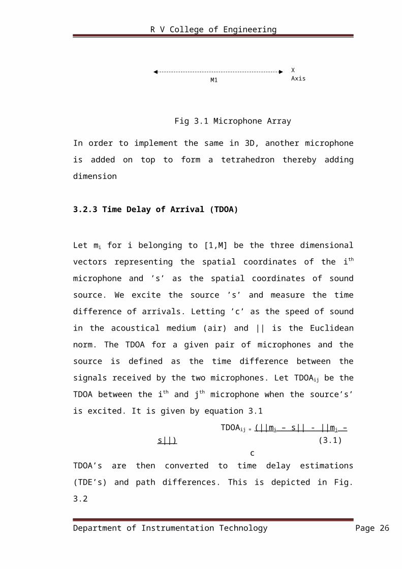
Fig 3.1 Microphone Array
In order to implement the same in 3D, another microphone is added on top to form a
tetrahedron thereby adding dimension
3.2.3 Time Delay of Arrival (TDOA)
Let mi for i belonging to [1,M] be the three dimensional vectors representing the
spatial coordinates of the ith microphone and ’s’ as the spatial coordinates of sound
source. We excite the source ’s’ and measure the time difference of arrivals. Letting
’c’ as the speed of sound in the acoustical medium (air) and || is the Euclidean norm.
The TDOA for a given pair of microphones and the source is defined as the time
difference between the signals received by the two microphones. Let TDOAij be the
TDOA between the ith and jth microphone when the source’s’ is excited. It is given by
equation 3.1
TDOAij = (||mi – s|| - ||mj – s||) (3.1) c
TDOA’s are then converted to time delay estimations (TDE’s) and path differences.
This is depicted in Fig. 3.2
Department of Instrumentation Technology Page 18
M1M1X Axis
R V College of Engineering
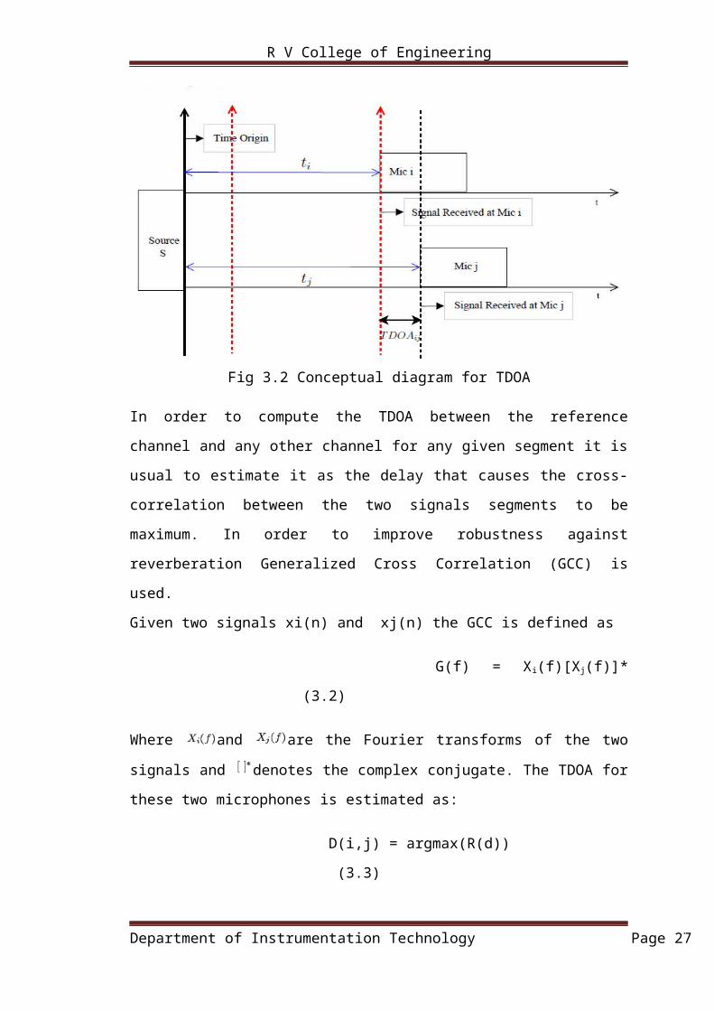
Fig 3.2 Conceptual diagram for TDOA
In order to compute the TDOA between the reference channel and any other channel
for any given segment it is usual to estimate it as the delay that causes the cross-
correlation between the two signals segments to be maximum. In order to improve
robustness against reverberation Generalized Cross Correlation (GCC) is used.
Given two signals xi(n) and xj(n) the GCC is defined as
G(f) = Xi(f)[Xj(f)]* (3.2)
Where and are the Fourier transforms of the two signals and denotes the
complex conjugate. The TDOA for these two microphones is estimated as:
D(i,j) = argmax(R(d)) (3.3)
In equation 3.3, R(d) is the inverse Fourier transform of Eq. (3.2). Maximum value of
R(d) corresponds to the estimated TDOA for that particular segment.
3.2.4 Algorithm to find Direction of Arrival
The lag at which the cross-correlation function has its maximum is taken as the time
delay between the two signals. Once TDOA estimation is performed, it is possible to
compute the position of the source through geometrical calculations. One technique
based on a linear equation system but sometimes, depending on the signals, the
Department of Instrumentation Technology Page 19
R V College of Engineering
system is ill-conditioned and unstable. For that reason, a simpler model based on far
field assumption is used [1]. Fig. 3.3 illustrates the case of a 2 microphone array with
a source in the far field.
Consider two microphones i and j placed at a distance Xij from each other. Tij is the
time delay of arrival found using the above method. On multiplying with the speed of
sound ‘c’, it gives the extra distance the sound source has to travel to reach
microphone i. On dropping a perpendicular, two angles of phi and theta are
subtended. u is a unit vector in the direction of the sound source.
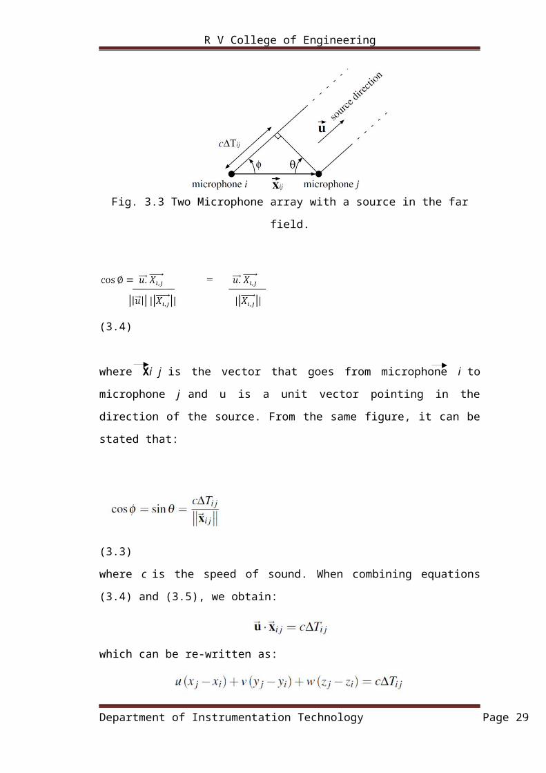
Fig. 3.3 Two Microphone array with a source in the far field.
(3.4)
where Xi j is the vector that goes from microphone i to microphone j and u is a unit
vector pointing in the direction of the source. From the same figure, it can be stated
that:
(3.3)
where c is the speed of sound. When combining equations (3.4) and (3.5), we obtain:
which can be re-written as:
Department of Instrumentation Technology Page 20
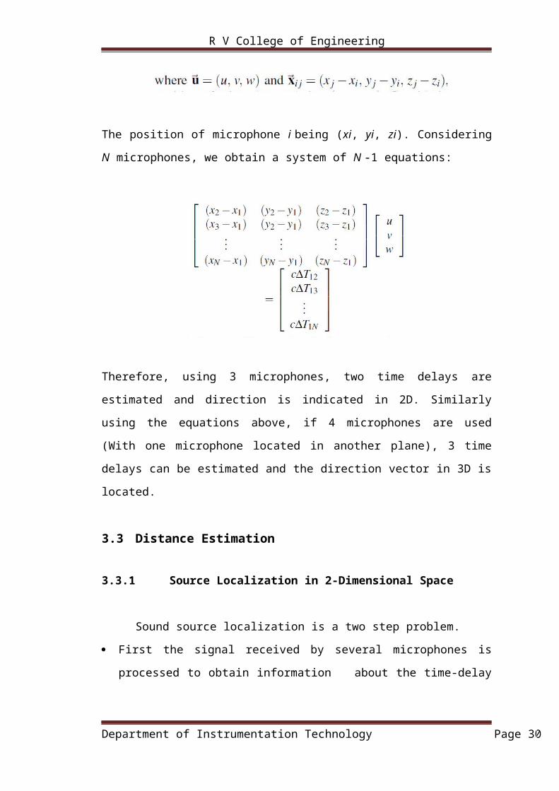
R V College of Engineering
The position of microphone i being (xi, yi, zi). Considering N microphones, we obtain
a system of N -1 equations:
Therefore, using 3 microphones, two time delays are estimated and direction is
indicated in 2D. Similarly using the equations above, if 4 microphones are used (With
one microphone located in another plane), 3 time delays can be estimated and the
direction vector in 3D is located.
3.3 Distance Estimation
3.3.1 Source Localization in 2-Dimensional Space
Sound source localization is a two step problem.
First the signal received by several microphones is processed to obtain
information about the time-delay between pairs of microphones. We use the
GCC PHAT method for estimating the time-delay.
The estimated time-delays for pairs of microphones can be used for getting the
location of the sound source.
3.3.2 Hyperbolic position location
By definition, a hyperbola is the set of all points in the plane whose location is
characterized by the fact that the difference of their distance to two fixed points is a
constant. The two fixed points are called the foci. In our case the foci are the
microphones. Each hyperbola consists of two branches. The emitter is located on one
Department of Instrumentation Technology Page 21
R V College of Engineering
of the branches. The line segment which connects the two foci intersects the
hyperbola in two points, called the vertices. The line segment which ends at these
vertices is called the transverse axis and the midpoint of this line is called the center
of the hyperbola [4].
The time-delay of the sound arrival gives us the path difference that defines a
hyperbola on one branch of which the emitter must be located. At this point, we have
infinity of solutions since we have single information for a problem that has two
degrees of freedom.
We need to have a third microphone, when coupled with one of the previously
installed microphones, it gives a second hyperbola. The intersection of one branch of
each hyperbola gives one or two solutions with at most of four solutions being
possible. Since we know the sign of the angle of arrivals, we can remove the
ambiguity.
Hyperbolic position location (PL) estimation is accomplished in two stages. The first
stage involves estimation of the time difference of arrival (TDOA) between the
sensors (microphones) through the use of time-delay estimation techniques. The
estimated TDOAs are then utilized to make range difference measurements. This
would result in a set of nonlinear hyperbolic range difference equations.
When the microphones are arranged in non-collinear fashion, the position location of
a sound source is determined from the intersection of hyperbolic curves produced
from the TDOA estimates. The set of equations that describe these hyperbolic curves
are non- linear and are not easily solvable. If the number of nonlinear hyperbolic
equations equals the number of unknown coordinates of the source, then the system is
consistent and a unique solution can be determined from iterative techniques. For an
inconsistent system, the problem of solving for the position location of the sound
source becomes more difficult due to non-existence of a unique solution
Department of Instrumentation Technology Page 22
R V College of Engineering
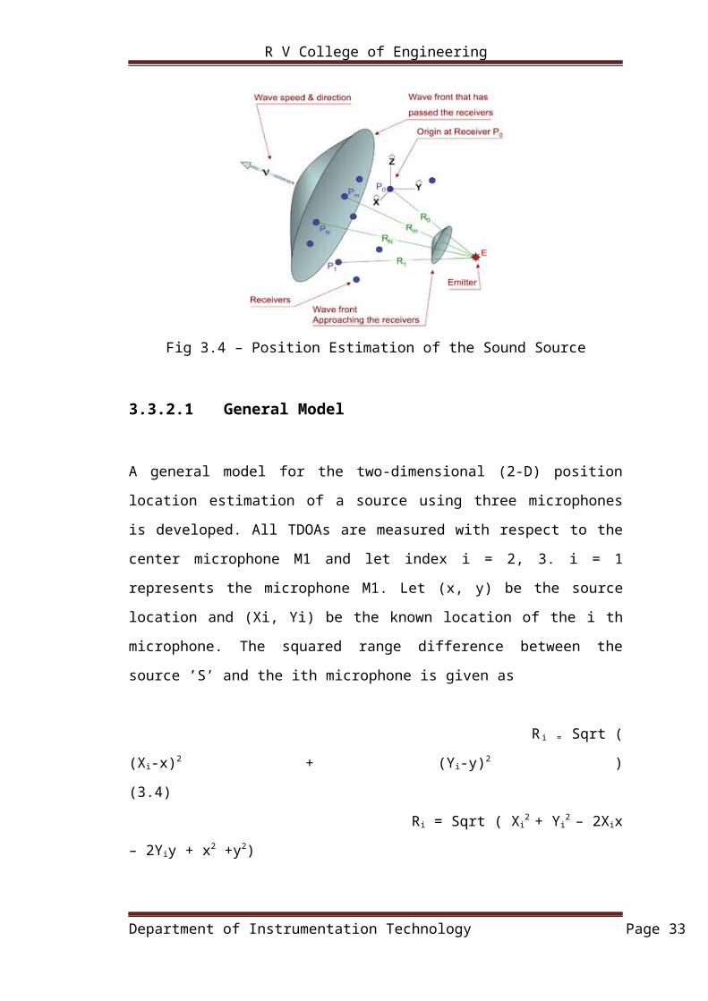
Fig 3.4 – Position Estimation of the Sound Source
3.3.2.1 General Model
A general model for the two-dimensional (2-D) position location estimation of a
source using three microphones is developed. All TDOAs are measured with respect
to the center microphone M1 and let index i = 2, 3. i = 1 represents the microphone
M1. Let (x, y) be the source location and (Xi, Yi) be the known location of the i th
microphone. The squared range difference between the source ’S’ and the ith
microphone is given as
Ri = Sqrt ( (Xi-x)2 + (Yi-y)2 ) (3.4)
Ri = Sqrt ( Xi2 + Yi
2 – 2Xix – 2Yiy + x2 +y2)
Using equation (3.4), the range difference between center microphone M1 and ith
microphone is
Ri,1 = cτi,1 = Ri – R1 (3.5)
Ri,1 = Sqrt( ( Xi – x)2 + (Yi – y)2) – Sqrt( (X1 – x)2 + (Y1 – y)2)
where c is velocity of sound, Ri,1 is the range difference distance between M1 and i th
microphone, R1 is the distance between M1 and sound source and τi,1 is the
estimated TDOA between M1 and i th microphone. This defines the set of nonlinear
hyperbolic equations whose solution gives the 2-D coordinates of the source.
Department of Instrumentation Technology Page 23
R V College of Engineering
3.3.2.2Position Estimation
To localize the source, we first estimate TDOA of the signal received by sensors i and
j using DFSE technique proposed in chapter 2. The technique measures TDOA’s
w.r.t. the first receiver, di, 1 = di – d1 for i = 2, 3... M. TDOA between receivers i and j
are computed from
di,j = di,1 − dj,1 where, i, j = 2, 3, ...,M
Let i = 2... M and source be at unknown position (x, y) and sensors at known locations
(xi, yi). The squared distance between the source and sensor i is
ri2= (xi − x)2 + (yi – y)2
= Ki − 2xix − 2yiy + x2 + y2 where i = 1, 2... M.
where Ki = xi2 + yi
2
If c is the speed of sound propagation, then
ri,1 = cdi,1 = ri − r1
define a set of nonlinear equations whose solution gives (x, y)
3.4 Hardware Design
3.4.1 cDAQ-9172
The cDAQ-9172 is an eight-slot NI CompactDAQ chassis that can hold up to eight C
Series I/O modules. This USB 2.0-compliant chassis operates on 11 to 30 VDC and
includes an AC/DC power converter and a 1.8 m USB cable.
The cDAQ-9172 has two 32-bit counter/timer chips built into the chassis. With a
correlated digital I/O module installed in slot 5 or 6 of the chassis, you can access all
the functionality of the counter/timer chip including event counting, pulse-wave
generation or measurement, and quadrature encoders.
Department of Instrumentation Technology Page 24
R V College of Engineering
3.4.2 Analog input module - NI 9234
The NI 9234 is a four-channel C Series dynamic signal acquisition module for making
high-accuracy audio frequency measurements from integrated electronic piezoelectric
(IEPE) and non-IEPE sensors with NI CompactDAQ system. The NI 9234 delivers
102 dB of dynamic range and incorporates software-selectable AC/DC coupling and
IEPE signal conditioning for accelerometers and microphones. The four input
channels simultaneously digitize signals at rates up to 51.2 kHz per channel with
built-in antialiasing filters that automatically adjust to your sampling rate.
3.4.3 Digital output module – NI 9472
The National Instruments NI 9472 is an 8-channel, 100 µs sourcing digital output
module for any NI CompactDAQ or CompactRIO chassis. Each channel is
compatible with 6 to 30 V signals and features 2,300 Vrms of transient overvoltage
protection between the output channels and the backplane. Each channel also has an
LED that indicates the state of that channel. With the NI 9472, you can connect
directly to a variety of industrial devices such as motors, actuators, and relays.
3.5 Assumptions and Limitations
We assume the following conditions under which location of sound source is
estimated:
Single sound source, infinitesimally small, omni directional source.
Reflections from the bottom of the plane and from the surrounding objects are
negligible.
No disturbing noise sources contributing to the sound field.
The noise source to be located is assumed to be stationary during the data
acquisition period.
Microphones are assumed to be both phase and amplitude matched and without
self-noise.
Department of Instrumentation Technology Page 25
R V College of Engineering
The change in sound velocity due to change in pressure and temperature are
neglected. The velocity of sound in air is taken as 330 m/sec.
Knowledge of positions of acoustic receivers and perfect alignment of the
receivers as prescribed by processing techniques.
Perfect solutions are not possible, since the accuracy depends on the following
factors:
Geometry of microphone and source.
Accuracy of the microphone setup.
Uncertainties in the location of the microphones.
Lack of synchronization of the microphones.
Inexact propagation delays.
Bandwidth of the emitted pulses.
Presence of noise sources.
Numerical round off errors.
Department of Instrumentation Technology Page 26
R V College of Engineering
Chapter - 4
IMPLEMENTATION OVERVIEW
Chapter - 4
IMPLEMENTATION OVERVIEW
4.1 Hardware and interfacing
In order to develop and evaluate the localization algorithms, it was necessary to first
test the hardware and write the required software interfaces. The hardware used were
five unidirectional microphones mounted on an array, NI compact DAQ along with
three modules, a servo motor which houses an indicator.
LabVIEW was used for interfacing with the hardware, as it provided a rich data
access toolbox. This also meant that no data conversion was required, as the
localization algorithms were implemented in LabVIEW.
Department of Instrumentation Technology Page 27
NI cDAQ 9172
R V College of Engineering
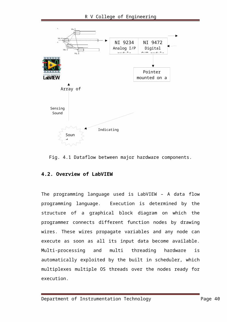
Fig. 4.1 Dataflow between major hardware components.
4.2. Overview of LabVIEW
The programming language used is LabVIEW – A data flow programming language.
Execution is determined by the structure of a graphical block diagram on which the
programmer connects different function nodes by drawing wires. These wires
propagate variables and any node can execute as soon as all its input data become
available. Multi-processing and multi threading hardware is automatically exploited
by the built in scheduler, which multiplexes multiple OS threads over the nodes ready
for execution.
NI LabVIEW is a graphical programming environment used on campuses all over the
world to deliver project-based learning to the classroom, enhance research
applications, and foster the next generation of innovators. With the intuitive nature of
graphical system design, educators and researchers can design, prototype and deploy
their applications.
LabVIEW programs/subroutines are called virtual instruments (VIs). Each VI has
three components: Block diagram, a front panel, and a connector pane. The last is
used to represent the VI in the block diagram of other, calling VIs. Controls and
indicators on the front panel allow an operator to input data into or extract data from a
Department of Instrumentation Technology Page 28
NI 9234Analog I/P
module
NI 9472Digital O/P
module
Pointer mounted on a servomotor
Sound source
Indicating direction of sound
Sensing SoundSignal
Array of microphones
R V College of Engineering
running virtual instrument. However, the front panel can also serve as a programming
interface. Thus a virtual instrument can either run as a program, with the front panel
serving a s a user interface, or, when dropped as a node onto the block diagram, the
front panel defined the inputs and outputs for the given node through the connector
pane, this implies that each VI can be easily tested before being embedded as a
subroutine into a larger program.
4.2.1 Front panel
Every user created VI has a front panel that contains the graphical interface with
which a user interacts. The front panel can house various graphical objects ranging
from simple buttons to complex graphs. Various options are available for changing
the look and feel of the objects on the front panel to match the application needs.
4.2.2 Block diagram
Nearly every VI has a block diagram containing some kind of program logic that
serves to modify data as it from sources to sinks. The block diagram houses a pipeline
structure of sources, sinks, VI’s, and structures wired together in order to define this
program logic.
Most importantly, every data source and sink from the front panel has its analog
source and sink on the block diagram. This representation allows the input values
from the user to be accessed from the block diagram. Likewise, new output values can
be shown on the front panel by code executed in the block diagram.
4.2 Programming using LabVIEW 11
There are 5 parts of graphical code in the program to make the VI and enable it to
localize the sound source in the most efficient manner. They are:
4.3.1 Microphone signal interface using NI DAQ Assistant.
4.3.2 Threshold detection of each signal
4.3.3 Finding time delay of arrival
Department of Instrumentation Technology Page 29
R V College of Engineering
4.3.4 Direction and distance estimation
4.3.5 Servo control
By joining and grouping these blocks appropriately, and running them continuously
will result in required software for the process.
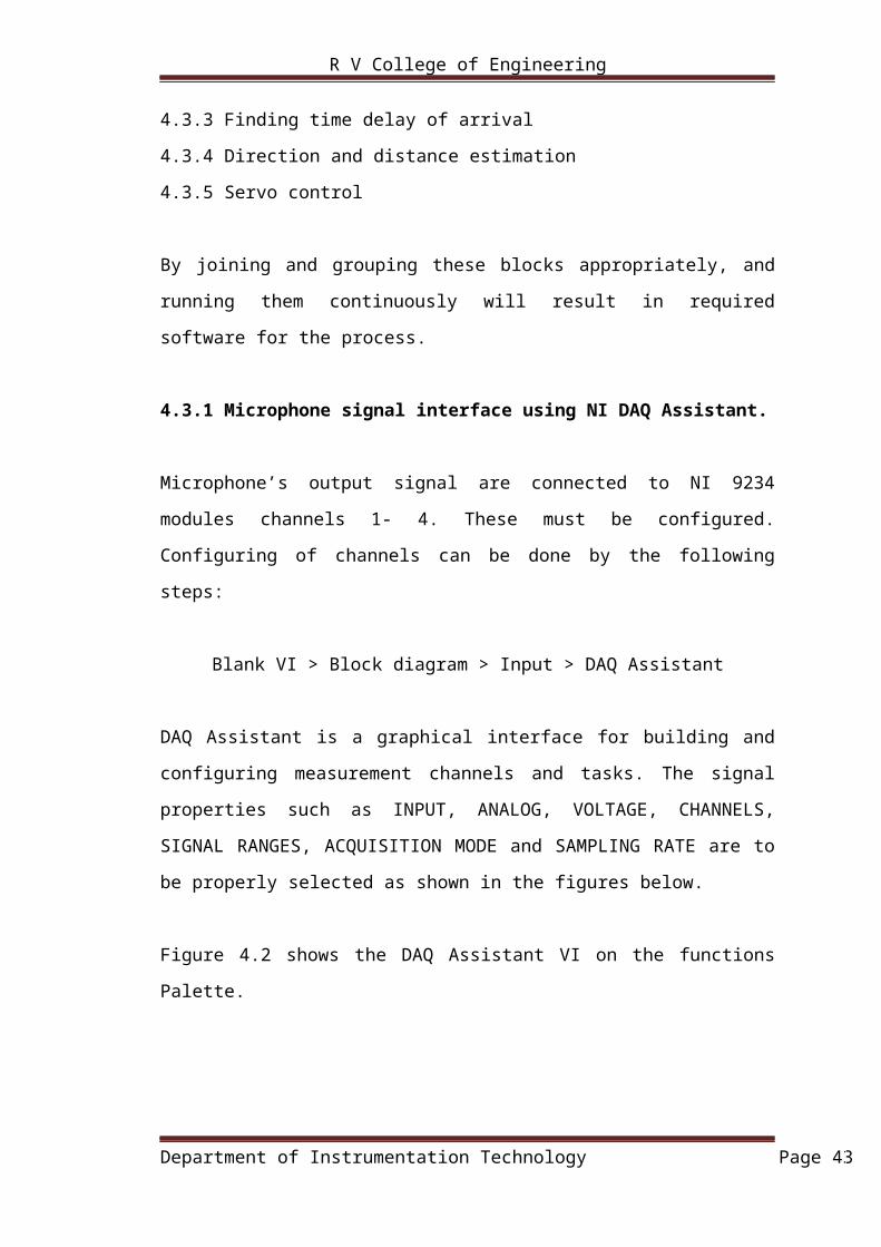
4.3.1 Microphone signal interface using NI DAQ Assistant.
Microphone’s output signal are connected to NI 9234 modules channels 1- 4. These
must be configured. Configuring of channels can be done by the following steps:
Blank VI > Block diagram > Input > DAQ Assistant
DAQ Assistant is a graphical interface for building and configuring measurement
channels and tasks. The signal properties such as INPUT, ANALOG, VOLTAGE,
CHANNELS, SIGNAL RANGES, ACQUISITION MODE and SAMPLING RATE
are to be properly selected as shown in the figures below.
Figure 4.2 shows the DAQ Assistant VI on the functions Palette.
Department of Instrumentation Technology Page 30
R V College of Engineering
Fig 4.2 Opening the DAQ assistant Palette
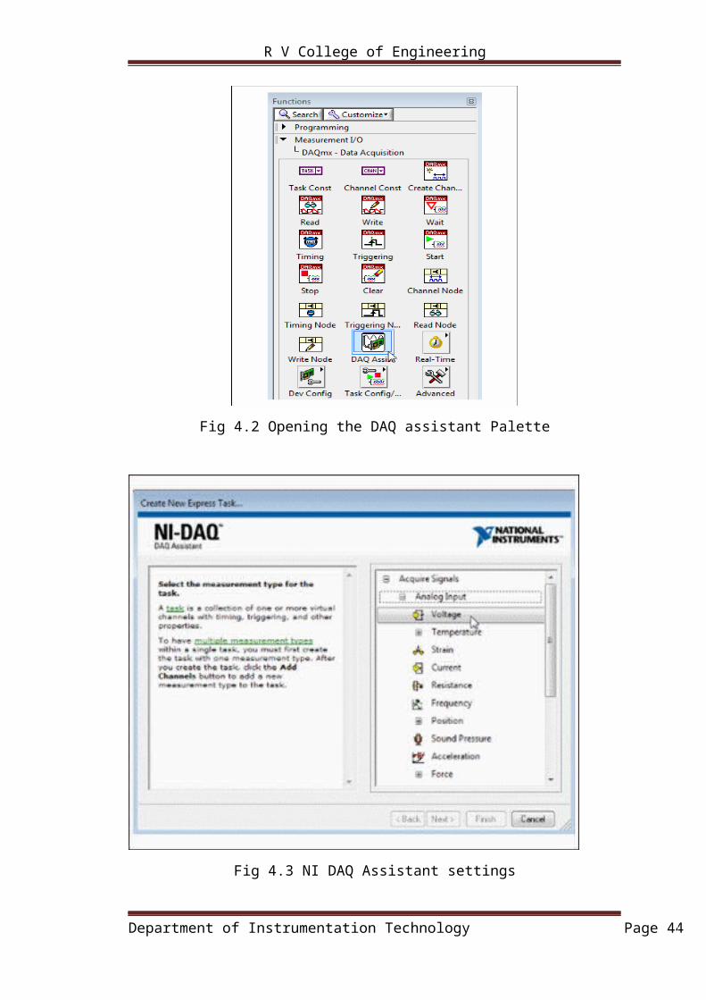
Fig 4.3 NI DAQ Assistant settings
Figure 4.3 indicates process for selection of each channel. This is the Create New
Express Task dialog box. Here you can choose which data acquisition device to use as
well as specify what type of data you want to acquire or generate. Select Generate
Signals»Analog Output»Voltage to specify that you want to generate the voltage of a
signal
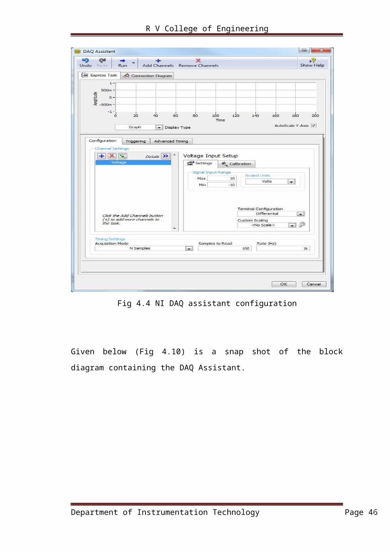
The DAQ Assistant dialog box allows you to edit the configurations you want to use
to measure and read the voltage. In figure 4.4, by clicking on the Add channel option,
the five channels connected to microphones can be added. The sampling rate can be
set as per requirement.
Department of Instrumentation Technology Page 31
R V College of Engineering
Fig 4.4 NI DAQ assistant configuration
Given below (Fig 4.10) is a snap shot of the block diagram containing the DAQ
Assistant.
Department of Instrumentation Technology Page 32
R V College of Engineering
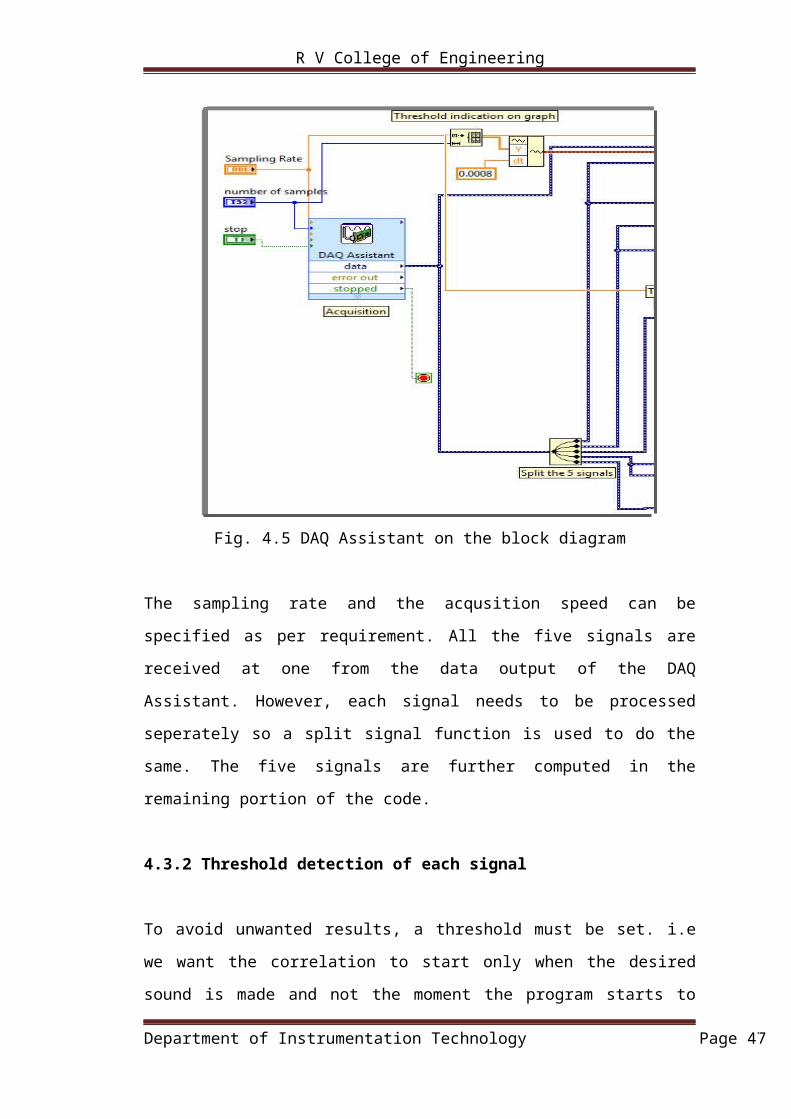
Fig. 4.5 DAQ Assistant on the block diagram
The sampling rate and the acqusition speed can be specified as per requirement. All
the five signals are received at one from the data output of the DAQ Assistant.
However, each signal needs to be processed seperately so a split signal function is
used to do the same. The five signals are further computed in the remaining portion of
the code.
4.3.2 Threshold detection of each signal
To avoid unwanted results, a threshold must be set. i.e we want the correlation to start
only when the desired sound is made and not the moment the program starts to run.
To ensure this, a threshold of 0.8 mV is set. So if any of the five microphones pick up
signals greater than 0.8 mV, the generalized cross correlation begins with respect to
the reference microphone. The set threshold can be seen in fig 4.12. When the signal
crosses the threshold as seen, the correlation starts.
Give below (Fig 4.11) is a snap shot of the thresohold detection portion of the code.
Department of Instrumentation Technology Page 33
R V College of Engineering
Fig. 4.6 Threshold detection
Fig 4.7 Waveforms generated on front panel
4.3.3 Finding time delay of arrival
Department of Instrumentation Technology Page 34
R V College of Engineering
Given in fig below is the sound signal received at two microphones simultaneously.
On close observation it can be seen that the signal is received at slightly different time
intervals. This is the time delay of arrival and has to be calculated. As the time
difference is very small, time stamping the reception of the signals at the microphones
will not give accurate results. In order to do this, generalized cross correlation is done
as explained in design. By cross correlating the signal, level of similarity of two
waveforms as a function of a time-lag applied to one of them is found. As an example,
consider two real valued functions f and g differing only by an unknown shift along
the x-axis. One can use the cross-correlation to find how much g must be shifted
along the x-axis to make it identical to f. The formula essentially slides the g function
along the x-axis, calculating the integral of their product at each position. When the
functions match, the value of (f*g) is maximized.
Fig. 4.8 Observed time delay of arrival between two microphones
Department of Instrumentation Technology Page 35
R V College of Engineering
Given below (Fig. 4.9) is a snap shot of the cross correlation done. The signal
received at each microphone is cross correlated with the reference microphone
(Microphone 1 at coordinate (0,0,0))
Fig. 4.9 Generalized cross correlation
Department of Instrumentation Technology Page 36
R V College of Engineering
4.3.4 Direction and distance estimation
Using the estimated time delay of arrival, specific algorithms are implemented to
estimate the position of sound source. Fig shows the direction estimation in 2D and
3D.
Fig. 4.10 Direction estimation
In figure 4.10, 1 indicates the coordinates of the microphones 2, 3 and 4. The
coordinates along with the difference in distance in solved as a linear equation for the
unknown matrix which is the direction vector indicating the direction of the sound
source. In 3, all the three components of the direction vector are extracted to indicate
direction in 3-D. The same is plotted on a 3-D graph. In 4, only two components of
direction vector are extracted to indicate direction in 2-D. The value obtained in
radians is converted to degrees.
Department of Instrumentation Technology Page 37
1. Coordinates of all five the microphones
4. Extracting first two elements of the direction vector and finding direction in 2D
3. Extracting all the three elements of direction vector and indicating the same on 3D graph
2. Solving linear equation
R V College of Engineering
In figure Fig 4.11, using the algorithm mentioned in the design, the distance to the
sound source can also be estimated using hyperbolic position estimation. It again
employs the time delay of estimation to formulate the equations.
Fig. 4.11 Distance estimation
4.3.5 Servo control
Once the direction is found, a servo motor is used to indicate the same. The duty cycle
of the servo motor and the direction values are interpolated to specify the rotation of
the servo motor for every degree. (Fig 4.12)
Fig. 4.12 Servo control
4.4 System Hardware
Figure 4.13 shows the major components in the physical set up of our system. The
microphones are mounted on the array structure to collect the sound signals. These
signals are sent to the PC via the CompactDAQ. In the PC, the program is run on
LabVIEW which does the processing and computation to obtain of the direction and
Department of Instrumentation Technology Page 38
R V College of Engineering
distance to the sound source. We will now describe each of the components in greater
detail.
Fig. 4.13 Set up
4.4.1 Microphone
The Panasonic RPVK21 Microphone (Fig 4.3) is a dynamic type, uni-directional
microphone. The microphone features an 80 Hz- 12 kHz frequency response and 55
dB/mW sensitivity which ensures that the sound is clear. It comes with a built-in
on/off switch that is easy to operate and an O.F.C output cable that measures 3 meters
in length.
Fig 4.14 Dynamic microphone
4.4.2 The microphone array
A stand for the microphones (figure 4.4), was constructed as per specifications, and
enabled the height of the entire array be adjusted from 1.5 -2 meter. For the purposes
of this project, a baseline of 1.5 meter was used. The servo was mounted below the
microphones on the central axis.
Department of Instrumentation Technology Page 39
R V College of Engineering
The purpose of the servo motor was to indicate the direction of the sound source on
one half of the 2-D plane. i.e 0-180 degrees.
Fig. 4.15 Microphone array
The coordinates of each microphone were fixed as shown in the figure below( Fig
4.5)
Fig. 4.16 Microphone coordinates
4.4.3 Data Acquisition
The cDAQ-9172 is an eight-slot NI CompactDAQ chassis that can hold up to eight C
Series I/O modules. It is connected to the Windows host computer connected over
USB. NI CompactDAQ serves as a flexible, expandable platform to meet the needs of
any electrical or sensor measurement system.
Department of Instrumentation Technology Page 40
(50,-35,0) (100,-35,0)
(-50,-35,0)
(0,-30,35)
(0,0,0)
R V College of Engineering
By placing instrumentation close to the test subject, electrical noise can be minimized
from the surroundings. This is because digital signals, used by USB are significantly
less susceptible to electromagnetic interference. Since the NI CompactDAQ is a small
rugged package, it can be easily placed close to the unit under test.
4.4.3.1 Modules
Analog input module - In our project, of the 8 slots, we have utilized 3 slots (slot1,
slot2, slot5) as shown in fig. Slot 1 and slot 2 are occupied by two NI 9234 modules.
NI 9234 are analog input modules capable of simultaneous acquisition. The five
microphones were connected to five channels respectively use BNC connections. The
required signal conditioning is done within the modules itself. Maximum allowable
sampling rate is 51.2kHz per channel. We have set our sampling rate as half of that i.e
25.6kHz per channel as during testing, our maximum frequency component does not
exceed 1000 hz. So 25.6kHz was found to be more than sufficient as over sampling
was resulting is excess data and hence slower processing. After the signals are
received by the analog input modules, they are sent for further processing to
LabVIEW. Here the algorithms which have already been discussed are implemented.
And once the direction and distance have been found, it is displayed on the front panel
as shown in fig 4.7.
Fig. 4.17 Front panel
Department of Instrumentation Technology Page 41
R V College of Engineering
Fig. 4.18 Hardware set up
Digital output module - Once the direction of sound source is found, the same is
indicated visually using a pointer which is mounted on a servo motor (fig. 4.8)
As shown in fig. the digital module NI 9274 is placed in slot 5 of the cDAQ chassis
(as slot 5 and 6 are the counter slots). The direction of sound source is given to the
digital module which in turn sends it to a servo motor in the form of a duty cycle
input.
Fig 4.19 Indicator
Department of Instrumentation Technology Page 42
Microphones 1,2,3,4 and 5 connected to channels 0 to 3 in the first module and channel 0 in the second using standard BNC connectors.
NI 9234 is connected to the counter 0 of the cDAQ in slot 5. PWM output is given from channel 3 of the DO module to the servo motor. Channels 8 and 9 are used for giving a Vsup of +5v.
NI cDAQ 9172 NI 9234 NI 9274
Servo motor
R V College of Engineering
4.5 Flow Chart
Department of Instrumentation Technology Page 43
Signals from five microphone array
Generalized cross correlation
Pick a peak
Estimate TDOA
Calculate path differences
Estimated path differences
Position estimation
Microphone locations
Estimated source location
Dimensions of coordinate system
R V College of Engineering
Chapter - 5
RESULTS AND DISCUSSION
Chapter - 5
Department of Instrumentation Technology Page 44
R V College of Engineering
RESULTS AND DISCUSSION
Experiments were done, using the algorithms described in the previous chapter, in
order to be able to gain insight into the operation of the system. A localization error
for each scenario was measured as the difference between the true angle, calculated
from the center of the array to the primary source, and the estimated angle as
predicted by the time delays. For this, it was assumed that the source was far away,
compared to the size of the array, and that the source could therefore fall on a straight
line from the array. This assumption was made and the errors calculated for both the
azimuthal and altitudinal angles of incidence and for each time-delay estimation
routine implemented. By its definition, the altitudinal angle may vary from +90 to -
90. The azimuthal angle may vary from 0 to 180.
5.1 Experimental set up
The source localization routine was tested by sound recording experiments done in a
laboratory. We setup a fixed coordinate system in the laboratory. Four microphones
were placed at the tips of an imaginary tetrahedral, whose sides are about 40 cm long.
A fifth microphone was placed as an extended arm of one of the microphones
(Fig.5.1). The microphones were hooked up to a computer, which ran a LabVIEW
program. The program saved five of signals from the microphones. Several sound
recording experiments were done by placing a source of sound at various locations in
the laboratory.
Fig. 5.1 Array structure
Department of Instrumentation Technology Page 45
Mic 4
Mic 1
Mic 2 Mic 5Mic 3
R V College of Engineering
We take into account both correlated noise and reverberation into account when
generating our test data. By setting a threshold, we eliminate the inherent noise and
pick up the most dominant sound in the room. The setup corresponds to a 6m-7m-
2.5m room, with five microphones placed at a distance from each other, 1m from the
floor and 1m from the 6m wall (in relation to which they are centered). The sound
source is generated from different positions.
The sampling frequency is 25.6kHz, and acquisition rate is 10kHz samples i.e. every
0.4 seconds. The sound source is generated using an air gun whose frequency range
lies within 500 – 1000 Hz. Thus a 25.6kHz sampling rate was sufficient.
A number of complications limit the potential accuracy of the system. Some of these
are due to physical phenomena that can never be corrected, and others are due to
inherent errors built into the processing, due to the design of the system. As
mentioned in the introduction, complications in locating the sound source that exist
outside of perfect conditions.
5.2 Experiment 3: Time delay of arrival
By estimating the measured sharp peak created by cross correlation of microphone
pairs, the time delay of arrival can be found. Given below is a figure showing the time
delay of arrival between microphones 1, 2 and 3. It can be seen in Fig 5.2 that ‘t1’ is
the extra time taken by the sound signal to reach microphone 2 and similarly ‘t3’ is
the extra time taken to reach microphone 3. Since the microphones are placed in a co-
linear fashion, on multiplying this time delay by the speed of sound, the distance
between the microphones is obtained. We have obtained the same using generalized
cross correlation. It was found to be highly accurate with +3 cm accuracy.
Fig. 5.2 Time delay of Arrival between microphone 1, 2, 3
5.3 Experiment 2: Direction of arrival
Department of Instrumentation Technology Page 46
Sound
Mic 3 Mic 2 Mic 1
t
t+Δt1
t+Δt2
R V College of Engineering
Once the time delay is estimated, it is used in a suitable algorithm as explained in
previous chapters to find the direction of sound source. For direction in 2D, consider
the plane formed by microphones 1, 2, 3 in figure 5.1. The table (5.1) shows the
estimated source location and the direction of the source. It gives the error when
measured in 2D. To normalize the error on both sides, instead of considering the
direction of the sound source from 0-180 degrees, 0 to (+90) and 0 to (-90) is
considered on both sides. The same is plotted as a graph in Figure 5.3.
Actual direction (Deg) Estimated direction (deg) %Error
10 12 20
20 23 15
30 35 10
50 46 6
80 79 3
90 90 0
-80 -75 4
-50 -45 8
-30 -37 11
-20 -22 14
-10 -16 19
Table 5.1
0 10 30 50 80 90 -80 -50 -30 -20 -100
5
10
15
20
25
Error
Figure 5.3
Department of Instrumentation Technology Page 47
ERROR
PERCENTAGE
ACTUAL TIME DELAY
R V College of Engineering
On observation it can be seen that the direction finding is most accurate in the range
of 80 – 100 degrees. As we go towards the extremes, the accuracy falls as the
microphones are unidirectional in nature. Hence, the signals are not picked up at its
best when it comes from the side. For best results, the sound source should be located
right in front of the microphone array. With omnidirectional microphones, this
constraint could be removed. But keeping the cost and availability in consideration,
we decided on the unidirectional microphones.
5.4. Experiment 3: Distance estimation
For distance finding in 2-D, the microphone array consists of 3 microphones. We
have conducted preliminary experiments with the 3 element microphone array. The
experiments involved acquiring signals from a sound source which is triggered by a
suitable mechanism. The source is located in a plane and its location is estimated
using the planar 3 microphone array.
The source is positioned at various places in 2-D space. The table 5.2 produces the
true, estimated source locations of the sound source. As mentioned in the chapter 3
Chan Ho’s linear array optimization method is utilized for solving the nonlinear
equations.
True distance (cm) Indicated distance (cm) %Error
10 13 30
50 55 10
75 79 5.3
100 104 4
120 125 4.1
150 157 4.6
180 189 5
210 221 5.23
250 275 10
Table 5.2
Department of Instrumentation Technology Page 48
R V College of Engineering
Distance to the sound source was found in 2-D. Table 5.2 tabulates the readings
obtained. On studying the same, varying levels of accuracy can be found. Larger
percentage of error is found when the sound source is placed too close to the
microphone or when the sound source is placed beyond 2 meters. So a safe range of
0.25 to 2 meters can be set.
The reason for this discrepancy is that if the sound source is placed too close to the
microphone array, it assumes a spherical approach. And our project works on the
assumption that sound signal travels in a straight manner i.e. the spherical nature of
the sound signal is not taken into account. Secondly, if the sound source is placed far
away, the sound signal reaches the microphones in an almost parallel manner so the
small time delay of arrival is not accounted for.
Department of Instrumentation Technology Page 49
R V College of Engineering
Chapter 6
CONCLUSIONS AND FUTURE WORK
Department of Instrumentation Technology Page 50
R V College of Engineering
Chapter 6
CONCLUSIONS AND FUTURE WORK
6.1 Conclusion
In this report we present an implementation of a sound-based localization technique
and introduce the platform we used in our lab. The report summarizes the basics of
sound-based localization as discussed in the literature. The process of time delay of
arrival estimation is explained. Then, the report explains the design which includes all
the algorithms, hardware, the assumptions and limitations. The implementation of the
concept is explained in detail. Finally, a comprehensive set of experimental results are
offered.
We find that in our current hardware deployment there are still many inevitable errors
in time of delay calculation. We proposed our algorithm which uses peak-weighted
goal function that detects sound source location in real time.
6.2 Future work
There are multiple factors which contribute towards errors in the sound-based
localization implementation. Future work will address reducing the impact of these
factors. These can be identified as follows:
(ii) Different materials exhibit different reflection and absorption coefficients. It has
been observed that the material of the floor between the microphone pair and the
sound source, affects the phase as well as amplitude of the signal received.
(iii) As the distance between the microphone pair and the sound source decreases, the
DOA estimates become coarser.
(iv)The position of sources of ambient noise in the room is important. This will affect
the nature of the percentage abnormality plot causing it to become non-symmetric.
(v) Position of reflective surfaces around the experimental setup contributes towards
the fluctuations.
Department of Instrumentation Technology Page 51
R V College of Engineering
(vi) Physical parameters such as speaker width and sensitivity of the microphone
contribute towards measurement errors.
(vii) The frequency response of the microphone elements also affects the fidelity of
the captured signal.
(viii) Accuracy of experimental setup and error due to elevation of microphone and
sound source are also factors which may cause errors.
The hyperbolic position location techniques presented in this thesis provides a general
overview of the capabilities of the system. Further research is needed to evaluate the
Dominant linear array algorithm for hyperbolic position location system. If improved
TDOA’s could be measured, the source position can be estimated very accurately.
Improving the performance of the algorithm for TDOA measurements reduces the
TDOA errors. The algorithm discussed for TDOA measurements is in its simplest
form.
Experiments were performed assuming that the source is stationary until all the
microphones have finished sampling the signals. Sophisticated multi-channel
sampling devices could be used to get rid of this stationary condition. While the
accuracy of the TDOA estimate appears to be a major limiting factor in the
performance of the hyperbolic position location system, the performance of the
hyperbolic position location algorithms is equally important. Position location
algorithms which are robust against TDOA noise and are able to provide
unambiguous solution to the set of nonlinear range difference equations are desirable.
For real-time implementations of source localization, closed-form solutions or
iterative techniques with fast convergence to the solution could be used. The trade-off
between computational complexity and accuracy exist for all position location
algorithms. The trade-off analysis through performance comparison of the closed-
form and iterative algorithms can be performed.
To find time delay only the most dominant peak is considered after performing
correlation. Exploring the possibility of taking advantage of second peak with particle
filtering must be done in order to get more reported sound source location data.
Department of Instrumentation Technology Page 52
R V College of Engineering
Chapter – 7
APPENDIX
Department of Instrumentation Technology Page 53
R V College of Engineering
BIBLIOGRAPHY
[1]Byoungho Kwon KAIST, Daejeon Gyeongho Kim ; Youngjin Park “Sound Source Localization Methods with Considering of Microphone Placement in Robot Platform”Robot and Human interactive Communication, 2007. RO-MAN 2007. The 16th IEEE International Symposium on 26-29 Aug. 2007
[2]Jean-Marc Valin, Franc¸ois Michaud, Jean Rouat, Dominic L´etourneau, “Robust Sound Source Localization Using a Microphone Array on a Mobile Robot”
[3]Y.T. Chan, senior member, IEEE, and K.C Ho, Member IEEE, “A simple and Efficient Estimator for Hyperbolic location”, IEEE transaction on signal processing, Vol 2, No. 8, Aug 1994.
[4] Ralph Bucher and D. Misra “A Synthesizable VHDL Model of the Exact Solution for Three-dimensional Hyperbolic Positioning System”, Volume 15 (2002), Issue 2, Pages 507-520.
[5] Johnson, Don H, Array Signal Processing: concepts and techniques.
[6] Lorraine Green Mazerolle, Ph.D, James Frank, Ph.D. “A Field Evaluation of the Shot spotter Gunshot Location System”
[7] Wang, H., Chu, P.: “Voice Source Localization for Automatic Camera Pointing System in Videoconferencing”. Proc. of IEEE Workshop on Applications of Signal Processing to Audio and Acoustics, Mohonk, New Paltz, NY, USA (1997)
[8] Biniyam Tesfaye Taddese, “ Sound Source Separation and Localization” Honors Thesis in Computer Science Macalester College, May 1st 2006.
[9] Alessio Brutti, Maurizio Omologo, Piergiorgio Svaizer, “Comparison Between Different Sound Source Localization Techniques Based On A Real Data Collection”, IEEE Conf. On HSCMA 2008.
[10] M. Brandstein and H. Silverman, “A practical methodology for speech localization with microphone arrays”, Technical Report, Brown University, November 13, 1996
[11] J. O. Pickels, “An Introduction to the Physiology of Hearing”, Academic Press, London, 1982.
Department of Instrumentation Technology Page 54