sources of currency depreciation in ghana
TRANSCRIPT

Southern Illinois University CarbondaleOpenSIUC
Theses Theses and Dissertations
12-1-2018
Sources of Currency Depreciation in GhanaHilarious Edem AnkuSouthern Illinois University Carbondale, [email protected]
Follow this and additional works at: https://opensiuc.lib.siu.edu/theses
This Open Access Thesis is brought to you for free and open access by the Theses and Dissertations at OpenSIUC. It has been accepted for inclusion inTheses by an authorized administrator of OpenSIUC. For more information, please contact [email protected].
Recommended CitationAnku, Hilarious Edem, "Sources of Currency Depreciation in Ghana" (2018). Theses. 2444.https://opensiuc.lib.siu.edu/theses/2444
SOURCES OF CURRENCY DEPRECIATION IN GHANA
By
Hilarious Edem Anku
B.S., University of Louisville, Kentucky, 2017
A Thesis
Submitted in Partial Fulfillment of the Requirements for the
Master of Science Degree
Department of Economics
in the Graduate School
Southern Illinois University Carbondale
December 2018
THESIS APPROVAL
SOURCES OF CURRENCY DEPRECIATION IN GHANA
By
Hilarious Edem Anku
A Thesis Submitted in Partial
Fulfillment of the Requirements
For the Degree of
Master of Science
in the field of Economics
Approved by:
Dr. AKM Mahbub Morshed, Chair
Dr. Sylwester Kevin
Dr. Scott Gilbert
Graduate School
Southern Illinois University Carbondale
November 6, 2018
i
AN ABSTRACT OF THE THESIS
Hilarious Edem Anku, for the Master of Science Degree in Economics, presented on November
6, 2018 at Southern Illinois University Carbondale.
TITLE: SOURCES OF CURRENCY DEPRECIATION IN GHANA
MAJOR PROFESSOR: Dr. AKM MAHBUB MORSHED
This paper investigates the factors driving the real exchange rate in the Ghanaian
economy. The paper aimed at finding the principal factor(s) that influence the real exchange rate
and explains the channels by which these factors exert their influence using standard empirical
methods of vector autoregressive (VAR) models. The paper established that inflation rate
differentials and interest rate differentials influence the exchange rate through the expectations
medium. Domestic and foreign money supplies which are exogenous macroeconomic variables
were also found to be important in the Ghanaian money market as far as the exchange rate
matters. The paper also highlighted how the great recession in the United States may have
affected the cedi/dollar rate of exchange after this economic event swept through the United
States generating spillover effects on economies around the world.

ii
ACKNOWLEDGEMENTS
I wish to extend my profound gratitude to the members of my thesis committee for going
the extra mile to help in the completion of this work. I also extend my appreciation to all the
professors of the department of Economics for their efforts in the teaching of Economics;
without their efforts I could not have produced this work.
To my colleague students in the department, I thank all of you for being some of the best
friends I have made in my academic life. Above all, your suggestions and encouragement were a
great booster when the going got tough.
And to all other staff of the department, I could not be more grateful for your work and
help each time it was needed. Thank you!
iii
TABLE OF CONTENTS
CHAPTER PAGE
ABSTRACT……………………………………………………………………………………….i
ACKNOWLEDGEMENTS……………………………………………………………………….ii
LIST OF TABLES………………………………………………………………………………..vi
LIST OF FIGURES…………………………………………………………………...................vii
CHAPTERS
CHAPTER 1 – Introduction……………………………………………………………….1
CHAPTER 2 – An Overview of Ghana’s Macroeconomy………………………………..3
2.1- The Political System, Government and Demographics…………………...3
2.2- General Growth Trends………………………………………....................4
2.3- Sectoral Analysis of the Ghanaian Economy……………………………...5
2.4- Notable Facts and Developments in Fiscal Policy………………………...7
2.5- Monetary System Facts and Developments………………………………10
2.6- Current Account Facts and Developments……………………………….14
CHAPTER 3- Literature Review………………………………………………………...16
3.1- Theoretical Review………………………………………………………16
3.2- Empirical Review of Ghana’s exchange rate……………………………17
iv
CHAPTER 4- Theoretical framework and Methodology………………………………..20
4.1- The Monetary Model…………………………………………………….20
4.2- Specification of the Empirical Model……………………………………20
CHAPTER 5- The Data, Data Sources and Empirical Methodology…............................22
CHAPTER 6- Presentation of Results…………………………………………………...24
6.1- Unit Root Tests…………………………………………………………...24
6.2- Johansen Cointegration Test Results……………………………………..24
6.3- Results of the Error Correction Model…………………………………...25
6.4- Diagnostic Test Results…………………………………………..............26
6.5- Test of Model Stability…………………………………………………...26
CHAPTER 7- Analysis of Results……………………………………………………….27
7.1- The Long Run…………………………………………………………….27
7.2- The Short Run…………………………………………………………….29
CHAPTER 8- Conclusion and Policy Implication………………………………………31
REFERENCES…………………………………………………………………………………..32
APPENDICES
APPENDIX A……………………………………………………………………………35
APPENDIX A.1………………………………………………………………………….36
v
APPENDIX A.2…………………………………………………………………………36
APPENDIX A.3…………………………………………………………………………37
APPENDIX A.4…………………………………………………………………………39
VITA……………………………………………………………………………………………..41
vi
LIST OF TABLES
TABLE PAGE
Table 1- ADF(k) Unit Root Test Results………………………………………………………...25
Table 2- Johansen Cointegration Test results……………………………………………………25
Table 3-Results of the Error Correction Model………………………………………………….26
Table 4- Diagnostic Test Results………………………………………………………………...27

vii
LIST OF FIGURES
FIGURE PAGE
Figure 1- Trend of the growth rate 1990 to 2016………………………………………………….5
Figure 2- Evolution of growth trends of the major
Sectors 1990 to 2016…………………………………………………………................6
Figure 3- The yearly fiscal deficit as a percent of GDP 1990 to 2016……………………………8
Figure 4- The national debt as a percent of GDP 1990 to 2016…………………………………..9
Figure 5- Government Spending versus Government
Revenue 1990 to 2016………………………………………………………………...10
Figure 6- Trend of the rate of inflation 1990 to 2016……………………………………………12
Figure 7- Exchange rate depreciation 1990 to 2016……………………………………………..14
Figure 8- Test of Model Stability………………………………………………………………...27

1
CHAPTER 1
INTRODUCTION
As a developing economy, many challenges confront Ghana. While the economy has
been making giant strides, some of these economic challenges prove to be very nimble and
difficult to contain. Speaking about difficult challenges in the Ghanaian economy, one that
frequently comes into sharp focus is the exchange rate. The exchange rate remains one of the
most hotly debated policy issues among experts in Ghana.
An important fact about the Ghanaian economy is its dependence on imports. Due to
rising capital investments of transition economies such as Ghana, this is not unusual.
International trade and finance as well as trade openness are all on the increase. These
developments and facts provide a reason why the exchange rate is such an essential factor in the
Ghanaian economy. This is a reason why this paper takes interest in the monetary matters of the
economy, the exchange rate being majorly interesting and intriguing for further study.
During the Bretton Woods era, the fixed exchange rate systems were in place and during
these periods, the exchange rate regime in the Ghanaian economy was very stable. The collapse
of the Bretton Woods forced a policy redirection in the monetary environment and Ghana
subsequently adopted the floating exchange rate system. The floating system, however, quickly
evolved into a managed floating system as time went by.
In view of the foregoing, the Ghanaian currency has experienced relative weakness by
means of incessant depreciations over time since the floating exchange rate system began. As
such, the natural question arises as follows: Why does the cedi always depreciate? For the

2
purposes of conducting a formal analysis I ask: What are the sources of currency depreciation in
Ghana?
In this paper, I intend to investigate the factors that determine the exchange rate in the
Ghanaian economy. In so doing, my aim is to focus on and isolate the most important factors that
influence the rate of exchange of the Ghanaian currency. I employ standard econometric
techniques to achieve this goal.
The rest of this paper is organized as follows: section 2 presents a general overview of the
Ghanaian economy. Section 3 reviews relevant literature on the subject matter. Section 4
presents the theoretical framework and methodology. Section 5 looks at the data, data sources
and empirical methodology. Section 6 presents the results. Section 7 is an analysis of the results.
Section 8 presents the conclusions and implications for policy.

3
CHAPTER 2
AN OVERVIEW OF GHANA’S MACROECONOMY
2.1 The Political System, Government and Demographics
Unlike many other countries in the West African sub-region, Ghana has a very stable
political climate, it is one of the most politically stable states in the region. Ghana has a unitary
system of government which means that, as far as economic and political decision making goes,
major policy initiatives in the country (political and economic) follow a top-down approach. The
government is made up of an executive branch, a legislature and a judiciary. All three branches
have specific roles in the economy, however, much of economic policy and planning falls on the
executive and legislative branches of the government.
In the region, the area covered by Ghana (the land mass) can be described as mid-size
relative to larger countries like Nigeria and Niger but the population of the country is second
behind Nigeria. It has always been the case in this region that Ghana’s population comes second
only to Nigeria. Official census figures recorded in 2010 put the population headcount at 24.65
million (Ghana Population and Housing Census Report, 2010). Official population estimate in
2018 is 29.58 million people, approximately 30 million people. The estimated labor force stands
at 14 million (World Bank Est., 2017).
With GDP per capita at $1,513, the World Bank classifies Ghana as a lower middle-
income country. As a developing nation in transition(United Nations Classification),
unemployment remains a major challenge. The unemployment rate in 2016 was 5.5 percent.
Even though this statistic looks quite good, it must be viewed with great caution because, as a
developing nation in transition, the unemployment rate is not a very reliable measure of the

4
health of the economy since such data is often notoriously inaccurate. As such, the level of
income may be a better measure of the health of the economy. In 2016, income per capita in PPP
dollars was $4,301 (World Bank).
2.2 General Growth Trends
Ghana’s economy suffered many setbacks in the 1980s mainly due to political upheavals
which precipitated fiscal and monetary imbalances. Referred to as the lost decade by Fischer
(1991), like most economies in Africa, the period between 1979 and 1989 was a period of
economic stagnation and negative growth in Ghana. As a result of stagnant growth, Ghana joined
the IMF’s structural adjustment program (SAP) in 1983. As part of the structural adjustment
program, an economic recovery program (ERP) was also implemented to restore the ailing
Ghanaian economy to positive growth. The economy responded well to many of the economic
recovery programs and growth bounced back in the 1990s.
Over the period 1990 to 2016, the Ghanaian economy expanded quite slowly but steadily.
In the 1990s, growth of the Ghanaian economy was not particularly strong. The average growth
rate over the decade spanning 1990 to 1999 was 4.27 percent. Though characterized by the
typical boom and bust of growth trends, growth of the Ghanaian economy was much stronger in
the millennium and beyond. Between 2000 and 2010, the growth rate averaged 5.78 percent, a
marked improvement over the previous decade (see figure 1).
In the millennium, the growth story of the Ghanaian economy continued. From 2008 to
2013, the growth rate averaged 8.76 percent. In this period, Ghana achieved its highest
economic growth rate of 14.05% in 2011 as the result of the combination of two factors: 1)
exportation of petroleum crude from its newly discovered oil fields. 2) high prices of Ghana’s

5
primary commodity exports in the international markets (Darko, 2015). However, gross domestic
product fell again, quite noticeably, in 2014, 2015 and 2016 largely due to an energy crisis that
rocked the economy.
Figure 1: Trend of the growth rate 1990-2016
Despite all the weaknesses of the Ghanaian economy, speaking in broad terms, Ghana’s
economy is one of the better performing economies in the West African sub-region. By measure
of gross domestic output, Ghana’s economy is the second largest behind Nigeria in the West
African Sub-region.
2.3 Sectoral Analysis of the Ghanaian Economy
Four major sectors are prominent in the Ghanaian economy. These are agriculture,
industry, manufacturing and the services sector. Agriculture was the mainstay of the Ghanaian
economy in the very early years contributing a lion share to total output. However, with the
Ghanaian economy undergoing major structural changes, agric is no longer the mainstay of the
0.00
2.00
4.00
6.00
8.00
10.00
12.00
14.00
16.00
19
90
19
91
19
92
19
93
19
94
19
95
19
96
19
97
19
98
19
99
20
00
20
01
20
02
20
03
20
04
20
05
20
06
20
07
20
08
20
09
20
10
20
11
20
12
20
13
20
14
20
15
20
16
GDP GROWTH(annual % Change)
GDP GROWTH(annual % Change)
6
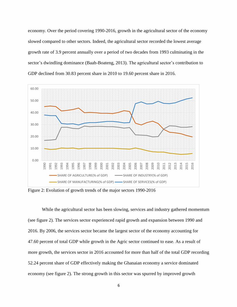
economy. Over the period covering 1990-2016, growth in the agricultural sector of the economy
slowed compared to other sectors. Indeed, the agricultural sector recorded the lowest average
growth rate of 3.9 percent annually over a period of two decades from 1993 culminating in the
sector’s dwindling dominance (Baah-Boateng, 2013). The agricultural sector’s contribution to
GDP declined from 30.83 percent share in 2010 to 19.60 percent share in 2016.
Figure 2: Evolution of growth trends of the major sectors 1990-2016
While the agricultural sector has been slowing, services and industry gathered momentum
(see figure 2). The services sector experienced rapid growth and expansion between 1990 and
2016. By 2006, the services sector became the largest sector of the economy accounting for
47.60 percent of total GDP while growth in the Agric sector continued to ease. As a result of
more growth, the services sector in 2016 accounted for more than half of the total GDP recording
52.24 percent share of GDP effectively making the Ghanaian economy a service dominated
economy (see figure 2). The strong growth in this sector was spurred by improved growth
0.00
10.00
20.00
30.00
40.00
50.00
60.00
19
90
19
91
19
92
19
93
19
94
19
95
19
96
19
97
19
98
19
99
20
00
20
01
20
02
20
03
20
04
20
05
20
06
20
07
20
08
20
09
20
10
20
11
20
12
20
13
20
14
20
15
20
16
SHARE OF AGRICULTURE(% of GDP) SHARE OF INDUSTRY(% of GDP)
SHARE OF MANUFACTURING(% of GDP) SHARE OF SERVICES(% of GDP)
7
performance in trade, hospitality and financial services (Alagidede, Baah-Boateng and Nketia-
Amponsah, 2013).
Industry on the other hand has also been expanding modestly behind services. In 1990,
this sector accounted for only 16.86 percent of GDP. This figure jumped to 28.16 percent of
GDP in 2016. This is another indication that while agriculture was on the decline, gains in
industry were being made. By 2016, the industrial sector which used to be third largest sector
came in second behind services. Between 1990 and 2016, most of the growth in the industrial
sector was driven largely by expansion in the extractive subsectors of the economy as mining
and construction activities witnessed accelerated growth (Baah-Boateng, 2013).
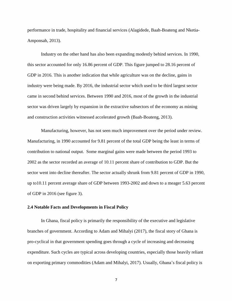
Manufacturing, however, has not seen much improvement over the period under review.
Manufacturing, in 1990 accounted for 9.81 percent of the total GDP being the least in terms of
contribution to national output. Some marginal gains were made between the period 1993 to
2002 as the sector recorded an average of 10.11 percent share of contribution to GDP. But the
sector went into decline thereafter. The sector actually shrunk from 9.81 percent of GDP in 1990,
up to10.11 percent average share of GDP between 1993-2002 and down to a meager 5.63 percent
of GDP in 2016 (see figure 3).
2.4 Notable Facts and Developments in Fiscal Policy
In Ghana, fiscal policy is primarily the responsibility of the executive and legislative
branches of government. According to Adam and Mihalyi (2017), the fiscal story of Ghana is
pro-cyclical in that government spending goes through a cycle of increasing and decreasing
expenditure. Such cycles are typical across developing countries, especially those heavily reliant
on exporting primary commodities (Adam and Mihalyi, 2017). Usually, Ghana’s fiscal policy is
8
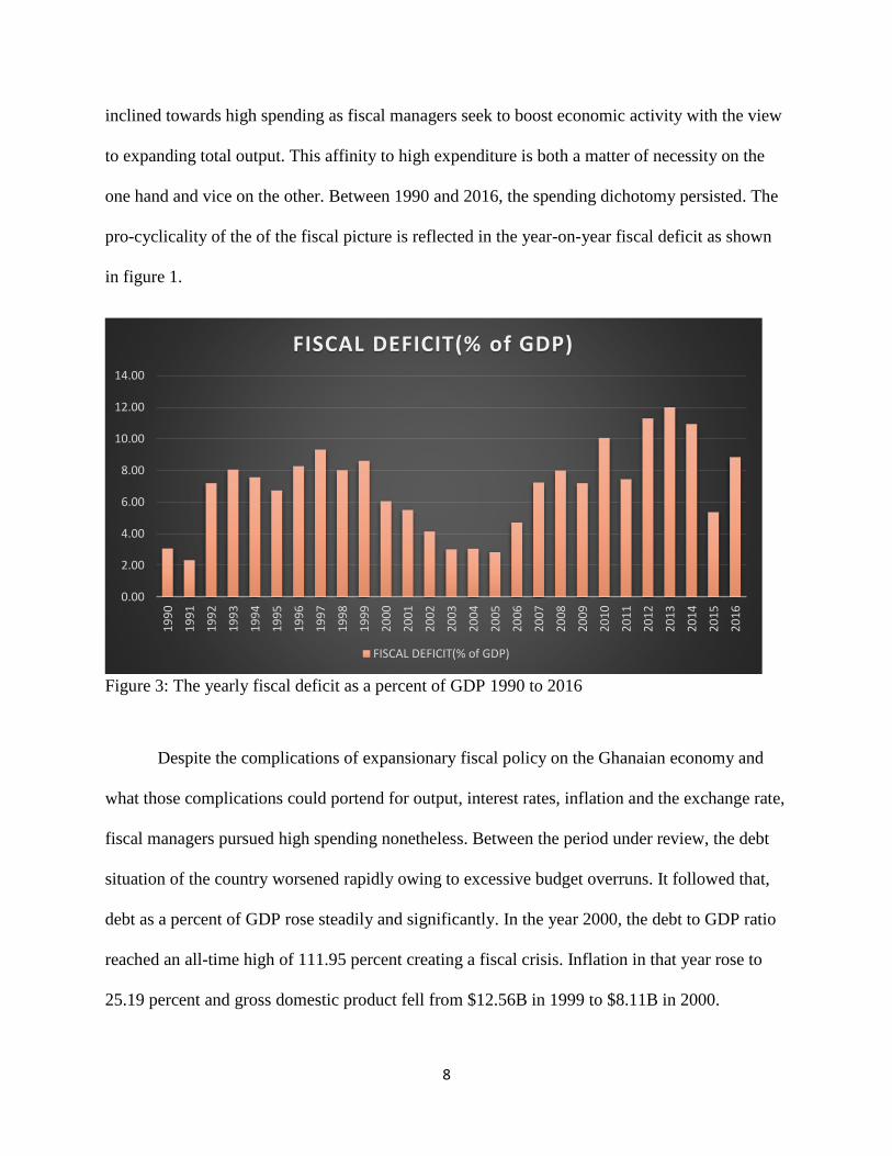
inclined towards high spending as fiscal managers seek to boost economic activity with the view
to expanding total output. This affinity to high expenditure is both a matter of necessity on the
one hand and vice on the other. Between 1990 and 2016, the spending dichotomy persisted. The
pro-cyclicality of the of the fiscal picture is reflected in the year-on-year fiscal deficit as shown
in figure 1.
Figure 3: The yearly fiscal deficit as a percent of GDP 1990 to 2016
Despite the complications of expansionary fiscal policy on the Ghanaian economy and
what those complications could portend for output, interest rates, inflation and the exchange rate,
fiscal managers pursued high spending nonetheless. Between the period under review, the debt
situation of the country worsened rapidly owing to excessive budget overruns. It followed that,
debt as a percent of GDP rose steadily and significantly. In the year 2000, the debt to GDP ratio
reached an all-time high of 111.95 percent creating a fiscal crisis. Inflation in that year rose to
25.19 percent and gross domestic product fell from $12.56B in 1999 to $8.11B in 2000.
0.00
2.00
4.00
6.00
8.00
10.00
12.00
14.00
19
90
19
91
19
92
19
93
19
94
19
95
19
96
19
97
19
98
19
99
20
00
20
01
20
02
20
03
20
04
20
05
20
06
20
07
20
08
20
09
20
10
20
11
20
12
20
13
20
14
20
15
20
16
FISCAL DEFICIT(% of GDP)
FISCAL DEFICIT(% of GDP)
9
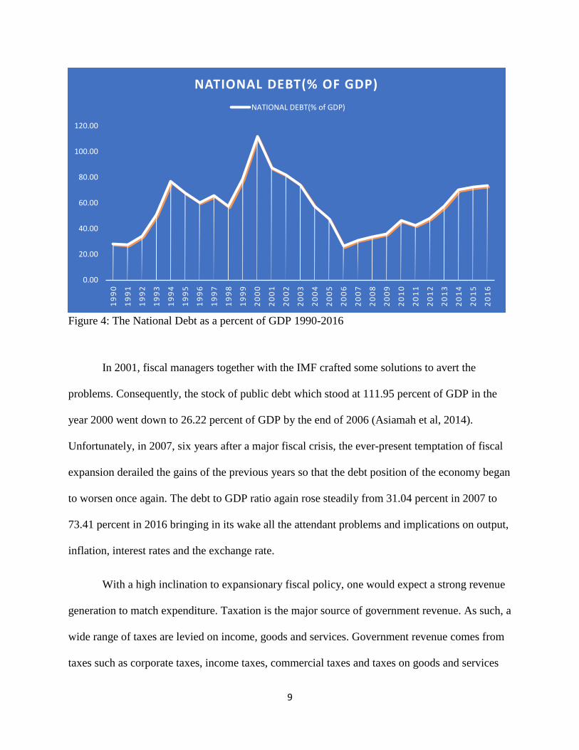
Figure 4: The National Debt as a percent of GDP 1990-2016
In 2001, fiscal managers together with the IMF crafted some solutions to avert the
problems. Consequently, the stock of public debt which stood at 111.95 percent of GDP in the
year 2000 went down to 26.22 percent of GDP by the end of 2006 (Asiamah et al, 2014).
Unfortunately, in 2007, six years after a major fiscal crisis, the ever-present temptation of fiscal
expansion derailed the gains of the previous years so that the debt position of the economy began
to worsen once again. The debt to GDP ratio again rose steadily from 31.04 percent in 2007 to
73.41 percent in 2016 bringing in its wake all the attendant problems and implications on output,
inflation, interest rates and the exchange rate.
With a high inclination to expansionary fiscal policy, one would expect a strong revenue
generation to match expenditure. Taxation is the major source of government revenue. As such, a
wide range of taxes are levied on income, goods and services. Government revenue comes from
taxes such as corporate taxes, income taxes, commercial taxes and taxes on goods and services
0.00
20.00
40.00
60.00
80.00
100.00
120.00
19
90
19
91
19
92
19
93
19
94
19
95
19
96
19
97
19
98
19
99
20
00
20
01
20
02
20
03
20
04
20
05
20
06
20
07
20
08
20
09
20
10
20
11
20
12
20
13
20
14
20
15
20
16
NATIONAL DEBT(% OF GDP)
NATIONAL DEBT(% of GDP)
10
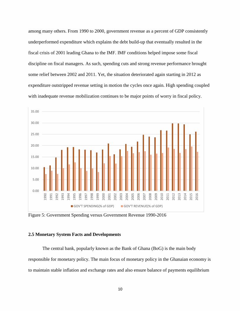
among many others. From 1990 to 2000, government revenue as a percent of GDP consistently
underperformed expenditure which explains the debt build-up that eventually resulted in the
fiscal crisis of 2001 leading Ghana to the IMF. IMF conditions helped impose some fiscal
discipline on fiscal managers. As such, spending cuts and strong revenue performance brought
some relief between 2002 and 2011. Yet, the situation deteriorated again starting in 2012 as
expenditure outstripped revenue setting in motion the cycles once again. High spending coupled
with inadequate revenue mobilization continues to be major points of worry in fiscal policy.
Figure 5: Government Spending versus Government Revenue 1990-2016
2.5 Monetary System Facts and Developments
The central bank, popularly known as the Bank of Ghana (BoG) is the main body
responsible for monetary policy. The main focus of monetary policy in the Ghanaian economy is
to maintain stable inflation and exchange rates and also ensure balance of payments equilibrium
0.00
5.00
10.00
15.00
20.00
25.00
30.00
35.00
19
90
19
91
19
92
19
93
19
94
19
95
19
96
19
97
19
98
19
99
20
00
20
01
20
02
20
03
20
04
20
05
20
06
20
07
20
08
20
09
20
10
20
11
20
12
20
13
20
14
20
15
20
16
GOV'T SPENDING(% of GDP) GOV'T REVENUE(% of GDP)

11
(Alagidede, Baah-Boateng and Nketia-Amponsah, 2013). Like most economies around the
world, the bank’s main tool in achieving macroeconomic targets is the policy rate. To this end, a
monetary policy committee meets periodically to review macroeconomic conditions and other
key economic indicators. This review of economic conditions informs monetary policy.
Over the years, the Ghanaian economy struggled at keeping stable inflation and exchange
rates. The difficulties of the economy in these respects are well documented. Regarding the
inflation rate, there were several instances in Ghana when the economy experienced
hyperinflation. For instance, in 1983, the inflation rate was 122.9 percent. Earlier in 1977 and
1981, the inflation rate was 116.5 percent respectively. Meanwhile, average inflation rate for
1976, 1978, 1979 and 1980 was 58.43 percent. From 1983, monetary authorities worked to bring
the situation under control. Subsequently, between 1990 and 2016, the rate of inflation slowed
down quite remarkably.
Figure 6: Trend of the rate of inflation 1990 to 2016
0.00
10.00
20.00
30.00
40.00
50.00
60.00
70.00
19
90
19
91
19
92
19
93
19
94
19
95
19
96
19
97
19
98
19
99
20
00
20
01
20
02
20
03
20
04
20
05
20
06
20
07
20
08
20
09
20
10
20
11
20
12
20
13
20
14
20
15
20
16
INFLATION RATE(CPI % change)
INFLATION RATE(CPI % change)
12
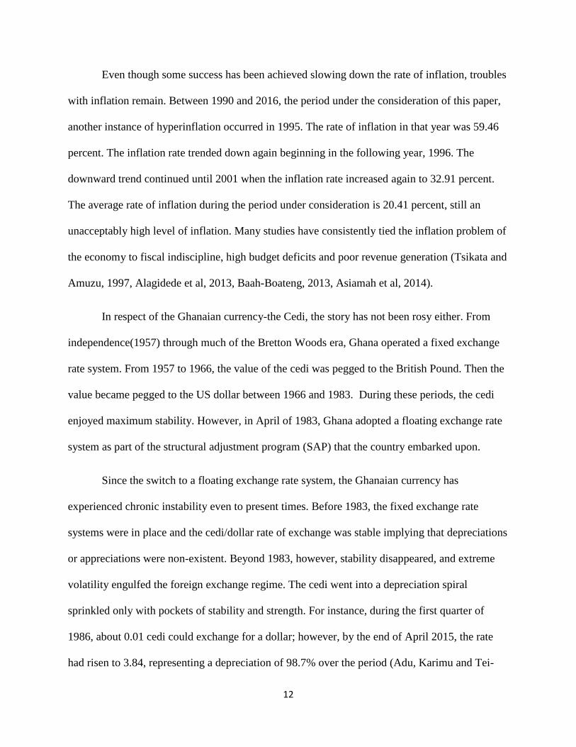
Even though some success has been achieved slowing down the rate of inflation, troubles
with inflation remain. Between 1990 and 2016, the period under the consideration of this paper,
another instance of hyperinflation occurred in 1995. The rate of inflation in that year was 59.46
percent. The inflation rate trended down again beginning in the following year, 1996. The
downward trend continued until 2001 when the inflation rate increased again to 32.91 percent.
The average rate of inflation during the period under consideration is 20.41 percent, still an
unacceptably high level of inflation. Many studies have consistently tied the inflation problem of
the economy to fiscal indiscipline, high budget deficits and poor revenue generation (Tsikata and
Amuzu, 1997, Alagidede et al, 2013, Baah-Boateng, 2013, Asiamah et al, 2014).
In respect of the Ghanaian currency-the Cedi, the story has not been rosy either. From
independence(1957) through much of the Bretton Woods era, Ghana operated a fixed exchange
rate system. From 1957 to 1966, the value of the cedi was pegged to the British Pound. Then the
value became pegged to the US dollar between 1966 and 1983. During these periods, the cedi
enjoyed maximum stability. However, in April of 1983, Ghana adopted a floating exchange rate
system as part of the structural adjustment program (SAP) that the country embarked upon.
Since the switch to a floating exchange rate system, the Ghanaian currency has
experienced chronic instability even to present times. Before 1983, the fixed exchange rate
systems were in place and the cedi/dollar rate of exchange was stable implying that depreciations
or appreciations were non-existent. Beyond 1983, however, stability disappeared, and extreme
volatility engulfed the foreign exchange regime. The cedi went into a depreciation spiral
sprinkled only with pockets of stability and strength. For instance, during the first quarter of
1986, about 0.01 cedi could exchange for a dollar; however, by the end of April 2015, the rate
had risen to 3.84, representing a depreciation of 98.7% over the period (Adu, Karimu and Tei-
13
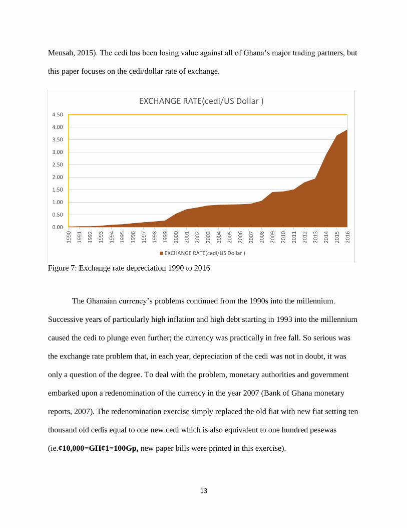
Mensah, 2015). The cedi has been losing value against all of Ghana’s major trading partners, but
this paper focuses on the cedi/dollar rate of exchange.
Figure 7: Exchange rate depreciation 1990 to 2016
The Ghanaian currency’s problems continued from the 1990s into the millennium.
Successive years of particularly high inflation and high debt starting in 1993 into the millennium
caused the cedi to plunge even further; the currency was practically in free fall. So serious was
the exchange rate problem that, in each year, depreciation of the cedi was not in doubt, it was
only a question of the degree. To deal with the problem, monetary authorities and government
embarked upon a redenomination of the currency in the year 2007 (Bank of Ghana monetary
reports, 2007). The redenomination exercise simply replaced the old fiat with new fiat setting ten
thousand old cedis equal to one new cedi which is also equivalent to one hundred pesewas
(ie.¢10,000=GH¢1=100Gp, new paper bills were printed in this exercise).
0.00
0.50
1.00
1.50
2.00
2.50
3.00
3.50
4.00
4.50
19
90
19
91
19
92
19
93
19
94
19
95
19
96
19
97
19
98
19
99
20
00
20
01
20
02
20
03
20
04
20
05
20
06
20
07
20
08
20
09
20
10
20
11
20
12
20
13
20
14
20
15
20
16
EXCHANGE RATE(cedi/US Dollar )
EXCHANGE RATE(cedi/US Dollar )

14
By redenominating the currency, the free fall of the cedi was arrested. The cedi/dollar
rate of exchange reversed suddenly to 0.94/1 whittling down exchange rate pressures in the
economy. Nevertheless, since these actions were not backed by any changes to key real variables
in the economy, the cedi began to depreciate again almost immediately (see figure 7). From 2008
onwards, the cedi lost value steadily and, in the process, any gains from the redenomination
exercise were quickly wiped away. Between 2013 and 2014 for example, the cedi depreciated by
28.74 percent cumulatively. In 2015, the cedi lost 15 percent in value against the dollar. The
cedi’s chronic depreciation problems still exist.
2.6 Current Account Facts and Developments
A major aspect of the Ghanaian economy relates to trade. Trade policy in the Ghanaian
economy is heavily tilted towards trade liberalization so that goods and services are freely
exchanged with the rest of the world. Ghana’s openness to trade reached a high of 116.05 percent
of GDP in the year 2000. Between 1990 and 2016, the average trade openness stood at 75.65
percent of GDP. These statistics underscore the importance of trade to the entire Ghanaian
economy. Trade remains at the heart of economic growth efforts around the world and much so
for Ghana (Tetteh, 2015).
A large chunk of the national income comes from the export of raw natural resources.
Commodities such as gold, cocoa beans and petroleum crude are the top exports. Lately,
technological improvements and growth resulted in agricultural goods like nuts, cashews and
cocoa paste (semi-finished cocoa beans) becoming an integral portion of the country’s export
mix. In 2016, these agricultural goods put together brought Ghana a total of $1.02B in export
earnings. This figure is the second largest earning behind the three leading exports; gold, cocoa

15
beans, and petroleum crude whose earnings totaled $12.80B. In the past five years, exports of
Ghana increased at an annual rate of 1.6 percent, from $14.6B in 2011 to $16.5B in 2016.
The Ghanaian economy is hugely import dependent mainly because the manufacturing
sector of the economy is still work in progress. Imports include both capital goods and
consumption goods with capital goods leading the pack. Between 1997 and 2005, imports as a
percent of GDP averaged 57.22 percent while between 2010 and 2016, the average imports to
GDP ratio was 49.67 percent. The list of goods that Ghana imports is exhaustive. However, the
leading imports are cars, delivery trucks, refined petroleum, cement and frozen fish. In 2016,
total imports amounted to $12.5B. Even though import pressure is present in the economy,
imports have been slowing since 2011 at a rate of 1.9 percent. Fortunately, exports maintained a
strong showing posting an annual growth rate of 1.6 percent since 2011. Subsequently, Ghana’s
economy posted a positive trade balance of $3.97B in 2016.
From this overview, it can be seen that the Ghanaian economy has been grappling with
major fiscal and monetary difficulties, a situation that implicates real variables like the exchange
rate, inflation rate, interest rates and output. It is also obvious that the Ghanaian currency faces
enormous challenges. It is also important to note that being an economy dependent on imports,
the exchange rate is critical in the economy. Meanwhile, the Ghanaian economy demonstrates
much potential especially in the areas of trade so that if difficulties and challenges in the
exchange rate space can be kept at bay, the economy can do even much better.
16
CHAPTER 3
LITERATURE REVIEW
3.1 Theoretical Review
The exchange rate is the price of domestic currency per unit of foreign currency. This is
the nominal value of the exchange rate. The real exchange rate requires a more rigorous
definition. According to Lansana Daboh (2010), the external real exchange rate concept (also
referred to as the purchasing power parity (PPP) definition) considers the real exchange rate as
the price of foreign goods relative to that of domestic goods, where both prices are expressed in
the same currency. That is, it defines the real exchange rate as the nominal exchange rate
adjusted for the relative price levels of foreign and domestic economy. This is given as follows:
𝑅𝐸𝑅 = e (𝑃∗
𝑃)
Where: RER is the real exchange rate, e is the nominal exchange rate, defined as domestic
currency per unit of foreign currency, P* is foreign price level and P is domestic price level. This
paper follows this definition of the real exchange rate.
In the literature, another theoretical matter of importance in the study of exchange rates is
the issue about which approach is most appropriate for measuring the exchange rate while at the
same time also appropriate for studying the factors that determine it. According to the
disequilibrium models of exchange rate determination (Dornbusch,1976), variations in both
nominal and real exchange rates are due to nominal disturbances which are expected to have a
transitory effect on the real exchange rate. On the contrary, disequilibrium models of exchange
rate determination rely on permanent real shocks to explain movements in the real and nominal
17
exchange rates (Stockman, 1987). However, the empirical studies following these theoretical
contributions have produced mixed results on the relative importance of real or nominal shocks
in accounting for movements in the real and nominal exchange rates (Adu et al, 2015).
Lastrapes (1992) reported that fluctuations in the real and nominal exchange rates are
primarily due to real shocks of all frequencies, thus lending support to equilibrium models of
Stockman (1987). Clarida and Gali (1994), however, found that nominal shocks were more
relevant in explaining movements in the real exchange rate. Many empirical works have either
confirmed the importance of real variables or affirmed nominal variables as more relevant in the
determination of the real exchange rate. For example, Chowdhury (2004), Hamori and Hamori
(2011) in their studies, found that real variables explained most of the variation in the real
exchange rate while Muntaz and Sunder-Plasmann (2013) reported a strong response of the
exchange rate to nominal shocks in their study of the exchange rates of the UK, Euro area and
Canada.
Since there is evidence from previous studies that both real and nominal shocks affect the
real exchange rate one way or the other, this paper combines both real and nominal variables to
investigate the sources of fluctuations in the rate of exchange between Ghana and the United
States (the cedi/dollar rate of exchange). The paper follows the assumptions of the PPP concept.
3.2 Empirical Review of Ghana’s exchange rate
Morrissey et al (2004) conducted a study that examined Ghana’s real exchange rate
response to capital inflows. The study employed vector autoregressive(VAR) models and the
Johansen system of equations approach to examine relationships between economic variables.
The estimation methods allowed for the interdependence and inter-relationships of
18
macroeconomic fundamentals to be identified in the determination of the exchange rate. Their
findings established that short-run movements in the exchange rate are inspired by changes in
trade volume. In the long run, they reported that capital flow is the most significant driver of the
real exchange rate in Ghana.
Owusu-Afriyie et al. (2004) derived a model of exchange rate determination for Ghana
and employed the technique of cointegration analysis to empirically investigate the principal
factors driving the Cedi/Dollar rate of exchange. The basic model was augmented with political
variables to examine potential impacts of politics on the exchange rate. Their results showed that
macroeconomic fundamentals are important determinants of the cedi/dollar rate of exchange.
The model also revealed that speculation was important in explaining exchange rate movements
but not so much for political variables.
Yemidi (2010) conducted a study focused on the variables that explain variation in the
exchange rate of the Ghanaian economy. He made use of quarterly data covering 24 years (1985
– 2008). His model, primarily based on the purchasing power parity concept, was done using
cointegration, granger causality test and vector error correction mechanism. Excessive
government expenditure coupled with past information on exchange rate, he noted, tend to have
dominant effect on the rate of exchange.
Fiagbor (2013) examined the relationship between the real effective exchange rate
(REER) and other macroeconomic variables in Ghana. This was to ascertain whether or not there
exist short run and long run causal relationships among the variables of interest. With a focus on
foreign aid, empirical models were developed for the real exchange rate. Data covering 32
years(1980 – 2011) were used. Vector autoregressive (VAR) and vector and error correction
19
(VEC) techniques were used in this study. The results showed that government expenditure,
foreign aid, terms of trade among others influenced the real exchange rate.
Sackey (2001) studied the factors that influence real exchange rate in Ghana. The
researcher postulated a relationship between the real exchange rate with commercial policy,
terms of trade, inflows of external aid (defined as real Net Official Development Assistance to
Ghana), government consumption, and technological progress as the explaining variables. The
cointegration approach was used to examine the aid-real exchange rate relationship employing
annual time series data covering the period 1962 - 1996. The study revealed that foreign aid
inflows results in real exchange rate depreciation.

20
CHAPTER 4
THEORETICAL FRAMEWORK AND METHODOLOGY
4.1 The monetary model
For the model in this paper, f is a function that defines the relationship between the
nominal exchange rate and other macroeconomic variables at time t. The model is expressed
such that the nominal exchange rate is a function of macroeconomic variables as follows:
ERt = f(Rt , USMt , GMt , GXt) ……………………………………………………………….4.1.1
where Rt, USMt, GMt and GXt are all related to the nominal exchange rate. Equation 4.1.1 can
further be expressed as follows:
ERt = Rtβ1 USMt
β2 GMtβ3 GXt
β4…………………………………………………………4.1.2
(The βs represent the degree to which each variable influences ERt). Taking log transformations
of equation 4.1.2 yields a linear equation as follows:
LnERt = β1LnRt + β2LnUSMt + β3LnGMt + β4LnGXt……………………………………….4.1.3
where βi = 𝜕𝑓
𝜕𝑥. Equation 4.1.3 contains both real and nominal macroeconomic variables. As
such, this model postulates that changes in both real and nominal variables cause the real
exchange rate to deviate from its equilibrium level.
4.2 Specification of the Empirical Model
To estimate and test the model above, an empirical formation of it was identified and
tested using traditional cointegration methods. Based on the theoretical model, the real exchange
21
rate is determined by the real interest rate, US money supply, Ghana money supply and
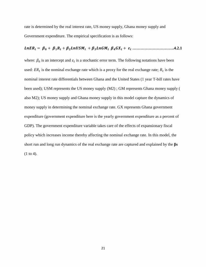
Government expenditure. The empirical specification is as follows:
𝑳𝒏𝑬𝑹𝒕 = 𝜷𝟎 + 𝜷𝟏𝑹𝒕 + 𝜷𝟐𝑳𝒏𝑼𝑺𝑴𝒕 + 𝜷𝟑𝑳𝒏𝑮𝑴𝒕 𝜷𝟒𝑮𝑿𝒕 + 𝜺𝒕 ………………………….4.2.1
where: 𝛽0 is an intercept and 휀𝑡 is a stochastic error term. The following notations have been
used: 𝐸𝑅𝑡 is the nominal exchange rate which is a proxy for the real exchange rate; 𝑅𝑡 is the
nominal interest rate differentials between Ghana and the United States (1 year T-bill rates have
been used); USM represents the US money supply (M2) ; GM represents Ghana money supply (
also M2); US money supply and Ghana money supply in this model capture the dynamics of
money supply in determining the nominal exchange rate. GX represents Ghana government
expenditure (government expenditure here is the yearly government expenditure as a percent of
GDP). The government expenditure variable takes care of the effects of expansionary fiscal
policy which increases income thereby affecting the nominal exchange rate. In this model, the
short run and long run dynamics of the real exchange rate are captured and explained by the βs
(1 to 4).
22
CHAPTER 5
THE DATA, DATA SOURCES AND EMPIRICAL METHODOLOGY
To test the validity of the model above, data covering the period 1990-2016 was collected
from three main sources: the World Bank, IMF and the Bank of Ghana. Data was not always
readily available for the demands of this study. Hence, some variables had to be proxied using
their closest data available. The real interest rate could not be observed, as such, 1 year T-bill
rates were used as proxy. (ie. The nominal interest rate differentials were used in the error
correction model)
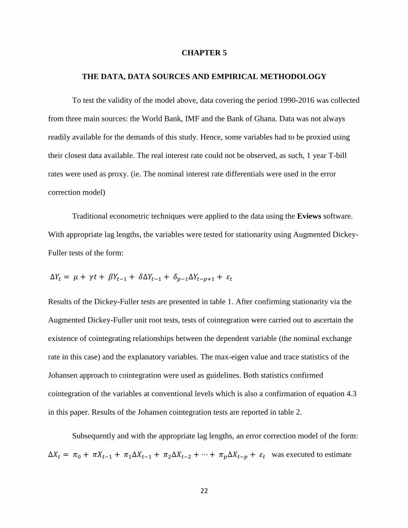
Traditional econometric techniques were applied to the data using the Eviews software.
With appropriate lag lengths, the variables were tested for stationarity using Augmented Dickey-
Fuller tests of the form:
∆𝑌𝑡 = 𝜇 + 𝛾𝑡 + 𝛽𝑌𝑡−1 + 𝛿∆𝑌𝑡−1 + 𝛿𝑝−1∆𝑌𝑡−𝑝+1 + 휀𝑡
Results of the Dickey-Fuller tests are presented in table 1. After confirming stationarity via the
Augmented Dickey-Fuller unit root tests, tests of cointegration were carried out to ascertain the
existence of cointegrating relationships between the dependent variable (the nominal exchange
rate in this case) and the explanatory variables. The max-eigen value and trace statistics of the
Johansen approach to cointegration were used as guidelines. Both statistics confirmed
cointegration of the variables at conventional levels which is also a confirmation of equation 4.3
in this paper. Results of the Johansen cointegration tests are reported in table 2.
Subsequently and with the appropriate lag lengths, an error correction model of the form:
∆𝑋𝑡 = 𝜋0 + 𝜋𝑋𝑡−1 + 𝜋1∆𝑋𝑡−1 + 𝜋2∆𝑋𝑡−2 + ⋯ + 𝜋𝑝∆𝑋𝑡−𝑝 + 휀𝑡 was executed to estimate
23
equation 4.4.1. Results of the error correction model are reported in table 3. This representation
summarizes the cointegration relationship between the variables.
To ascertain the statistical accuracy of the model, diagnostic tests were conducted to
check for any possible statistical errors. Serial LM test confirmed no serial correlation, Breusch-
Pagan-Godfrey test of heteroskedasticity also confirmed homoskedastic errors, the histogram
normality test returned normality of residuals, the CUSUM stability test confirmed stability of
the model at the 5% level. Results of diagnostic tests are reported in the results section.

24
CHAPTER 6
PRESENTATION OF RESULTS
6.1 UNIT ROOT TESTS
TABLE 1: ADF(k) UNIT ROOT TEST RESULTS
LEVELS FIRST DIFFERENCES
VARIABLE k A B
ER 1 -3.644 -1.062
GX 1 -1.902 -2.624
RD 1 -2.356 -2.750
LnUSM 1 -2.741** -2.881
LnGM 0 -4.702*** -5.553***
1% crt value -3.711 -4.356
5% crt value -2.981 -3.595
VARIABLE k A B
ΔLnER 1 -3.903*** -4.103**
ΔGX 1 -5.310*** -5.396***
ΔRD 1 -6.098*** -5.955***
ΔLnUSM 1 -6.393*** -6.283***
ΔLnGM 1 -6.455*** -6.292***
1% crt value -3.724 -4.374
5% crt value -2.986 -3.603
Notes:
1.k is the number of lags included in ADF Test
2. A = ADF with constant only; B = ADF with constant and trend
3.*** denotes significance at 1% level and **denotes significance at 5% level
6.2 JOHANSEN COINTEGRATION TEST RESULTS
TABLE 2
Null Trace Statistic 5% Crt value Max-Eigen Statistic 5% Crt value
None* 137.1088 69.8189 70.1630 33.8769
Atmost 1* 66.9458 47.8561 29.8222 27.5843
At most 2* 37.1236 29.7971 17.7747 21.1316
Atmost 3* 19.3489 15.4947 14.6301 14.2646
Atmost 4* 4.7188 3.8415 3.8415 3.8415
*Trace test indicates 5 cointegrating equations at the 5% significance level
*Max-Eigen value test indicates 2 cointegrating equations at the 5% significance level

25
6.3 RESULTS OF THE ERROR CORRECTION MODEL
TABLE 3
VARIABLE COEFFICIENT AND T-STATISTIC
ΔLnER(-1) -0.106 (-0.547)
ΔLnER(-2) 0.035 (0.194)
ΔRD(-1) 0.004 (0.936)
ΔRD(-2) -0.009 (-2.410)**
ΔGX(-1) -0.026 (-2.001)*
ΔGX(-2) 0.012 (1.090)
ΔLnUSM(-1) 0.046 (2.007)*
ΔLnUSM(-2) 0.044 (2.083)*
ΔLnGM(-1) 0.506 (5.040)***
ΔLnGM(-2) 0.071 (1.118)
Constant 0.215 (3.845)***
ECT(-1) -0.151 (-5.338)***
R2 = 0.79 Adjusted R2 = 0.59 DW = 1.95 F- Statistic = 3.98
Prob(F-statistic) = 0.012
Notes: T-Statistics are in brackets; * denotes significance at the 10% level, ** denotes
significance at the 5% level and ***denotes significance at the 1% level.
26
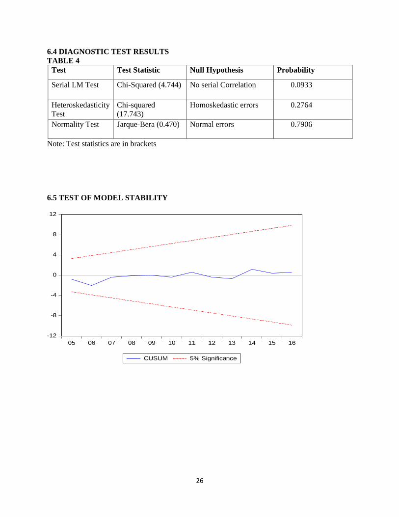
6.4 DIAGNOSTIC TEST RESULTS
TABLE 4
Test Test Statistic Null Hypothesis Probability
Serial LM Test Chi-Squared (4.744) No serial Correlation 0.0933
Heteroskedasticity
Test
Chi-squared
(17.743)
Homoskedastic errors 0.2764
Normality Test Jarque-Bera (0.470) Normal errors 0.7906
Note: Test statistics are in brackets
6.5 TEST OF MODEL STABILITY
-12
-8
-4
0
4
8
12
05 06 07 08 09 10 11 12 13 14 15 16
CUSUM 5% Significance
27
CHAPTER 7
ANALYSIS OF RESULTS
From the results, it is imperative to notice that the fundamentals of the Ghanaian
economy are key to maintaining a stable exchange rate regime. Specifically, fundamental
economic variables such as the inflation rate, the interest rate and money supply are critical in
this regard. The results in this study show that changes in the rate of inflation, the interest rate or
money supply ultimately affect the cedi’s rate of exchange. As such, volatility or stability of the
cedi can also be traced back to these economic variables.
The error correction term in this study is negative and statistically significant at the 1%
level. This result confirms that a long run equilibrium rate of exchange exists for the cedi. The
error correction term also reveals that deviations from the long run equilibrium which occur in
the previous period are corrected at an adjustment speed of 15.1%. This result also affirms that
the exchange rate tends to revert to its long run equilibrium level after deviating from it. As
noted in the literature review section, further analysis of these results in the following paragraphs
follow the assumptions of the PPP concept.
7.1 The Long Run
As mentioned earlier and supported by the error correction model, changes in the
inflation rate, the interest rate and money supply can cause the exchange rate to deviate from the
long run equilibrium path. In the long run, prices in the economy are adjustable, hence, the price
level is flexible. An important economic variable shown in this study to be of paramount
importance in determining the exchange rate is money supply. In this respect, when the Bank of
Ghana announces an increase in the money supply, money supply does not grow immediately;

28
the prevailing level of money supply in the economy remains operational momentarily (at least
for a brief period of time). The price level, on the other hand, responds instantly (The price level
increases as demand rises) causing real money supply to fall.
This phenomenon means that real money demand outweighs real money supply briefly.
To maintain equilibrium between real money supply and real money demand, interest rates rise
to restore equilibrium in the money market. Since interest rates are rising, one would expect the
exchange rate to appreciate but such is not the case. This is because the rising interest rate is a
result of an increasing price level which increasing price level is interpreted by economic agents
to mean higher price levels in the future, all else being constant. In other words, economic agents
come to expect higher inflation rates even in the future; economic agents sensing loss of
purchasing power(due to the rising price level) move their asset holdings into dollar denominated
assets causing demand for the dollar to rise. The domestic price per unit of the dollar
subsequently rises culminating in a depreciating cedi each time this phenomenon repeats itself.
The observed exchange rate data of the Ghanaian economy also affirms the results above.
Even though interest rates are relatively higher in the Ghanaian economy, the exchange rate does
not appreciate as would be expected. Rather, we observe a sustained depreciation of the currency
most of the time. As such, it can be said that expectations about inflation are a major driving
force of the cedi’s rate of exchange so that deviations (extreme volatility, mostly depreciation)
from the long run equilibrium are chiefly influenced by money supply. The rate of inflation, the
major vehicle through which disturbances to the exchange rate find expression becomes a critical
signal upon which economic agents act invariably resulting in depreciation(s) or appreciation(s)
of the currency.

29
7.2 The Short Run
Interest rate differential(lagged) is statistically significant in the short run. In the short
run, the equilibrium exchange rate is determined by interest rate differentials. Prices do not
adjust immediately in the short run; hence the price level is deemed inflexible in this
circumstance. However, the exchange rate (which is also a price) is more amenable to change, as
such, it can adjust freely in the short run to equilibrate aggregate demand and aggregate supply.
When government expenditure increases, output increases and disposable income rises. Such
increases in income raises the demand for real money balances. All else being constant, rising
incomes must be accompanied by interest rate increases resulting in a violation of the
requirements of interest rate parity in exchange rate determination. Consequently, the exchange
rate adjusts correspondingly to restore equilibrium temporarily (short run).
In the case of Ghana, the scattered pockets of currency appreciation are a result of interest
rate differentials. In the Ghanaian economy, government spending is one preferred way of
increasing domestic output. The resultant increases in output raises demand for real money
balances which pushes interest rates up. Accordingly, interest rates are quite high in the
Ghanaian economy. In these cases, demand for the cedi rises causing it to appreciate as investors
seek to profit from the high interest rates in the short run. It must be noted that this situation is
not the norm (especially against major currencies like the US dollar) as the Ghanaian currency
depreciates more than it appreciates. However, when the cedi appreciates, this is the mechanism
by which it does.
Zakari and Owusu-Afriyie (2004) in their paper found that increases in US money supply
strengthened (appreciation) the cedi in the short run. This result is consistent with theory;
however, it fails to take into account major events like the great recession (2008 economic

30
downturn) which affected economies around the world. This is not a weakness of their work
since their study was done prior to the great recession which happened in 2008.
The results in this study show that increases in US money supply depreciates the
Ghanaian cedi. This is evidenced in the lagged US money supply variables in the error correction
model which are significant at the 10% level. This result reflects the effects of the happenings in
the US money market on the cedi-dollar rate of exchange. To deal with the economic downturn
in the US caused by the great recession, US money supply increased sharply causing interest
rates to fall to historic lows in the United States. The dollar weakened in this process. But
consumption and investment in the United States increased resulting in a steady rise in US
output. On the flip side, volume effect and value effect dynamics played out in the Ghanaian
economy as a result of the happenings in the United States. Demand for US goods is always high
in economies like Ghana hence increased US output and a weak dollar means increased demand
for US goods in Ghana resulting in increased upward pressure on the nominal exchange rate
hence a depreciating cedi as shown by the positive and statistically significant lagged effects of
US money supply in this model.

31
CHAPTER 8
CONCLUSION AND POLICY IMPLICATION
This study was primarily focused on identifying the major factors that account for
exchange rate movements in Ghana. To this end, data covering the period between 1990 and
2016 was collected and analyzed. The vector error correction model was adopted as the preferred
empirical method in analyzing the data.
The results reveal that a long run equilibrium exists for the exchange rate in Ghana and
the exchange rate fluctuates around this equilibrium level. Factors such as the money supply
(both domestic and foreign), the inflation rate differentials, interest rate differentials and
government expenditure are important economic variables in determining the long run
equilibrium exchange rate.
In the long run, expectations play a major role in determining the exchange rate. By this
way, inflation rate differential was found to be the major vehicle by which expectations drive
movements in the exchange rate of the Ghanaian economy. Specifically, higher levels of domestic
inflation rate relative to foreign inflation rate result in a depreciation of the cedi against the dollar. In
the short run, however, differences in interest rate is the major driver of exchange rate
fluctuations. Relatively higher interest rates in the Ghanaian economy brings about a
strengthening of the Ghanaian cedi.
In all, the major takeaway from the results of this study is that the fundamentals of the
Ghanaian economy are important in the determination of the exchange rate. For the Ghanaian
economy to enjoy some stability in the exchange rate market, macroeconomic planning needs to
target the inflation rate and keep it in check.
32
REFERENCES
Adu, G., Karimu, A., & Mensah, J. T. (2015). An Empirical Analysis Of Exchange Rate
Dynamics And Pass-Through Effects On Domestic Prices. International Growth Center.
Alagidede, P., & Ibrahim, M. (2016). On The Causes And Effects Of Exchange Rate Volatility
on Economic Growth, Evidence From Ghana. Journal Of African Business.
Bacchetta, P., & Wincoop, E. V. (2000). Does Exchange Rate Stability Increase Trade And
Welfare. Econpapers.
BoG. (2007). Bank of Ghana Annual Reports. Accra, Ghana: Bank of Ghana.
Canetti, E., & Greene, J. (1991). Monetary Growth And Exchange Rate Depreciation As Causes
Of Inflation In African Countries: An Empirical Analysis. International Monetary Fund .
Christian, D. (2015). Determinants of Economic Growth in Ghana. Leibniz Information Centre
for Economics.
Claessens, S., & Kose, A. (2017). Asset Prices And Macroeconomic Outcome: A survey. The
World Bank .
Daboh, L. (2010). Real Exchange Rate Misalignment In The West African Monetary Zone.
Journal of Monetary And Economic Integration.
Devereux, M., & Lane, P. (2003). Understanding Bilateral Exchange Rate Volatility. Journal Of
International Economics .
Elkhafif, M. (2003). Exchange Rate Policy And Currency Substitution: The Case of Africa's
Emerging Economies. African Development Review.
Enders, W. (1995). Applied Econometric Time Series. United States : John Wiley & Sons, Inc.

33
Ferretti, G. M., & Razin, A. (2000). Current Account Reversals and Currency Crises: Empirical
Regularities. In P. Krugman, Currency Crises (pp. p. 285 - 323). Chicago: University of Chicago
Press.
Gyima-Brempong, K. (1991). Export Instability And Economic Growth in Sub-Saharan Africa.
University Of Chicago.
Hau, H. (2002). Real Exchange Rate Volatility And Economic Openness: Theory And Evidence.
Journal of Money, Credit And Banking.
J.O, A., S.A, Y., & Olatoke, A. (2014). The Impact Of Exchange Rate Fluctuation On The
Nigerian Economic Growth. International Journal Of Academic Research In Business And
Social Sciences.
Joseph, K. (2012). Determination of Real Exchage Rate Misalignment for Ghana. Institute of
economic affairs ghana.
Mumuni, Z., & afriyie, e. o. (2004). Determinants of The Cedi/Dollar Rate of Exchange in
Ghana: A Monetary Approach. Bank of Ghana Working Papers.
Ojo, A., & Alege, P. (2014). Exchange Rate Fluctuations And Macroeconomic Performance In
Sub-Saharan Africa: A Panel Cointegration Analysis. Asian Economic And Financial Review.
Opoku-Afari, M., Morissey, O., & Lloyd, T. (2004). Real excahnge rate response to capital
inflows: A dynamic analysis for Ghana. Center for Research in Economic Development and
International Trade.
Razafimahefa, I. (2012). Exchange Rate Pass-Through in Sub-Saharan African Ecconomies And
its Determinants. International Monetary Fund Working Papers.
34
Reinhart, C., & Rogoff, K. (2002). FDI to Africa:The Role Of Price Stability And Currency
Instability. International Monetary Fund.
Rodrik, D. (2008). The Real Exchange Rate And Economic Growth. Brooking Institution,
Havard University.
Sackey, H. A. (2001). External Aid Inflows And the Real Exchange Rate in Ghana. African
Economic Research Consortium.
Summers, L. (2000). International Financial Crises: Causes, Prevention And Cures. The
American Economic Review.
Tenreyro, S. (2007). On The Trade Impact Of Nominal Exchange Rate Volatility. Journal Of
Development Economics.

APPENDICES
35
Appendix A
Definition of the real exchange rate
The nominal exchange rate is the price of domestic currency per unit of foreign currency. The
real exchange rate is defined as the nominal exchange rate adjusted for the relative foreign and
domestic price levels following Lansana Daboh (2010). Hence:
𝑅𝐸𝑅 = 𝑒(𝑃∗/𝑃) where
RER = real exchange rate
e = nominal exchange rate
P*= foreign Price level
P = domestic Price level
Appendix A.1
The monetary model
The monetary model proposes that the real exchange rate in the Ghanaian economy at time t is a
function of the real interest rate (Rt), US money supply (USMt), Ghana money supply (GMt) and
Ghana government expenditure (GXt).
ERt = f(Rt , USMt , GMt , GXt). Changes in Rt, USMt, GMt and GXt impact the nominal
exchange rate thereby affecting the real exchange rate. Expanding the function f and taking log
transformations of it yields a linear equation (ie. Eqn 4.1.3).
To estimate equation 4.1.3, the following specification was used:
LnERt = β0 + β1LnRt + β2LnUSMt + β3LnGMt + β4LnGXt + εt
Further analysis of the model and results follow the assumptions of the PPP concept.
36
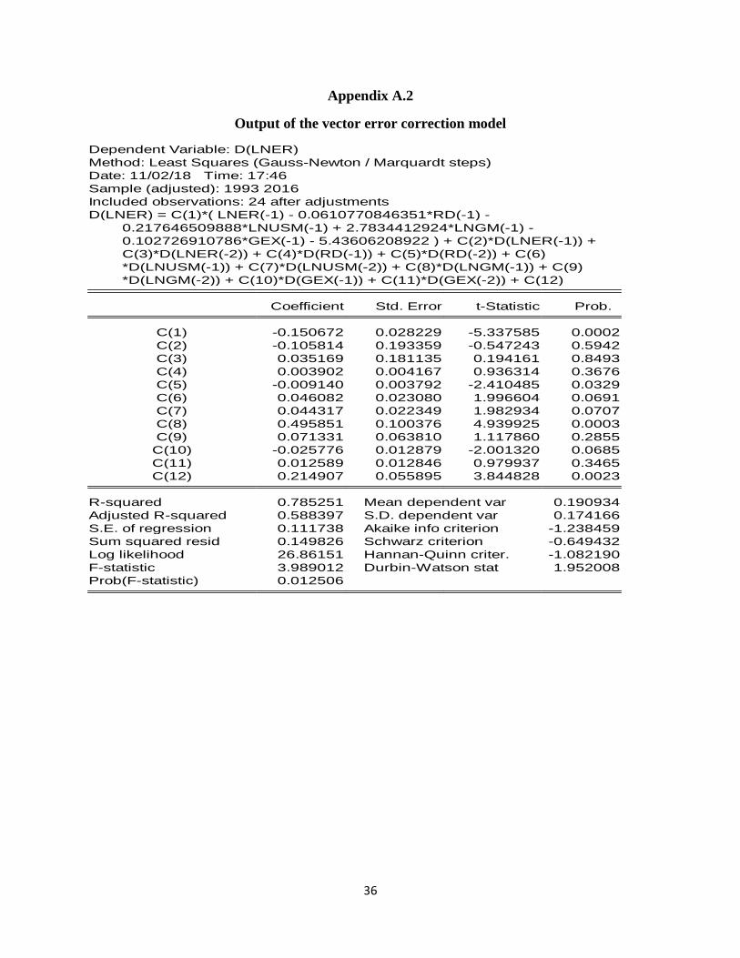
Appendix A.2
Output of the vector error correction model
Dependent Variable: D(LNER)
Method: Least Squares (Gauss-Newton / Marquardt steps)
Date: 11/02/18 Time: 17:46
Sample (adjusted): 1993 2016
Included observations: 24 after adjustments
D(LNER) = C(1)*( LNER(-1) - 0.0610770846351*RD(-1) -
0.217646509888*LNUSM(-1) + 2.7834412924*LNGM(-1) -
0.102726910786*GEX(-1) - 5.43606208922 ) + C(2)*D(LNER(-1)) +
C(3)*D(LNER(-2)) + C(4)*D(RD(-1)) + C(5)*D(RD(-2)) + C(6)
*D(LNUSM(-1)) + C(7)*D(LNUSM(-2)) + C(8)*D(LNGM(-1)) + C(9)
*D(LNGM(-2)) + C(10)*D(GEX(-1)) + C(11)*D(GEX(-2)) + C(12)
Coefficient Std. Error t-Statistic Prob.
C(1) -0.150672 0.028229 -5.337585 0.0002
C(2) -0.105814 0.193359 -0.547243 0.5942
C(3) 0.035169 0.181135 0.194161 0.8493
C(4) 0.003902 0.004167 0.936314 0.3676
C(5) -0.009140 0.003792 -2.410485 0.0329
C(6) 0.046082 0.023080 1.996604 0.0691
C(7) 0.044317 0.022349 1.982934 0.0707
C(8) 0.495851 0.100376 4.939925 0.0003
C(9) 0.071331 0.063810 1.117860 0.2855
C(10) -0.025776 0.012879 -2.001320 0.0685
C(11) 0.012589 0.012846 0.979937 0.3465
C(12) 0.214907 0.055895 3.844828 0.0023
R-squared 0.785251 Mean dependent var 0.190934
Adjusted R-squared 0.588397 S.D. dependent var 0.174166
S.E. of regression 0.111738 Akaike info criterion -1.238459
Sum squared resid 0.149826 Schwarz criterion -0.649432
Log likelihood 26.86151 Hannan-Quinn criter. -1.082190
F-statistic 3.989012 Durbin-Watson stat 1.952008
Prob(F-statistic) 0.012506

37
Appendix A.3
Graphs of variables at Level (A = ADF with constant only; B= ADF with constant and
trend)
(A) (B)
(A) (B)
0
1
2
3
4
90 92 94 96 98 00 02 04 06 08 10 12 14 16
ER
0
1
2
3
4
90 92 94 96 98 00 02 04 06 08 10 12 14 16
ER
10.0
12.5
15.0
17.5
20.0
22.5
25.0
27.5
30.0
90 92 94 96 98 00 02 04 06 08 10 12 14 16
GX
10.0
12.5
15.0
17.5
20.0
22.5
25.0
27.5
30.0
90 92 94 96 98 00 02 04 06 08 10 12 14 16
GX

38
(A) (B)
(A) (B)
(A) (B)
0
5
10
15
20
25
30
35
40
90 92 94 96 98 00 02 04 06 08 10 12 14 16
RD
0
5
10
15
20
25
30
35
40
90 92 94 96 98 00 02 04 06 08 10 12 14 16
RD
-3
-2
-1
0
1
2
3
90 92 94 96 98 00 02 04 06 08 10 12 14 16
LnUSM
-3
-2
-1
0
1
2
3
90 92 94 96 98 00 02 04 06 08 10 12 14 16
LnUSM
2.4
2.6
2.8
3.0
3.2
3.4
3.6
3.8
4.0
4.2
90 92 94 96 98 00 02 04 06 08 10 12 14 16
LnGM
2.4
2.6
2.8
3.0
3.2
3.4
3.6
3.8
4.0
4.2
90 92 94 96 98 00 02 04 06 08 10 12 14 16
LnGM
39
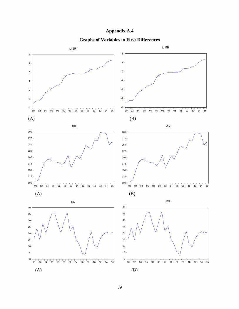
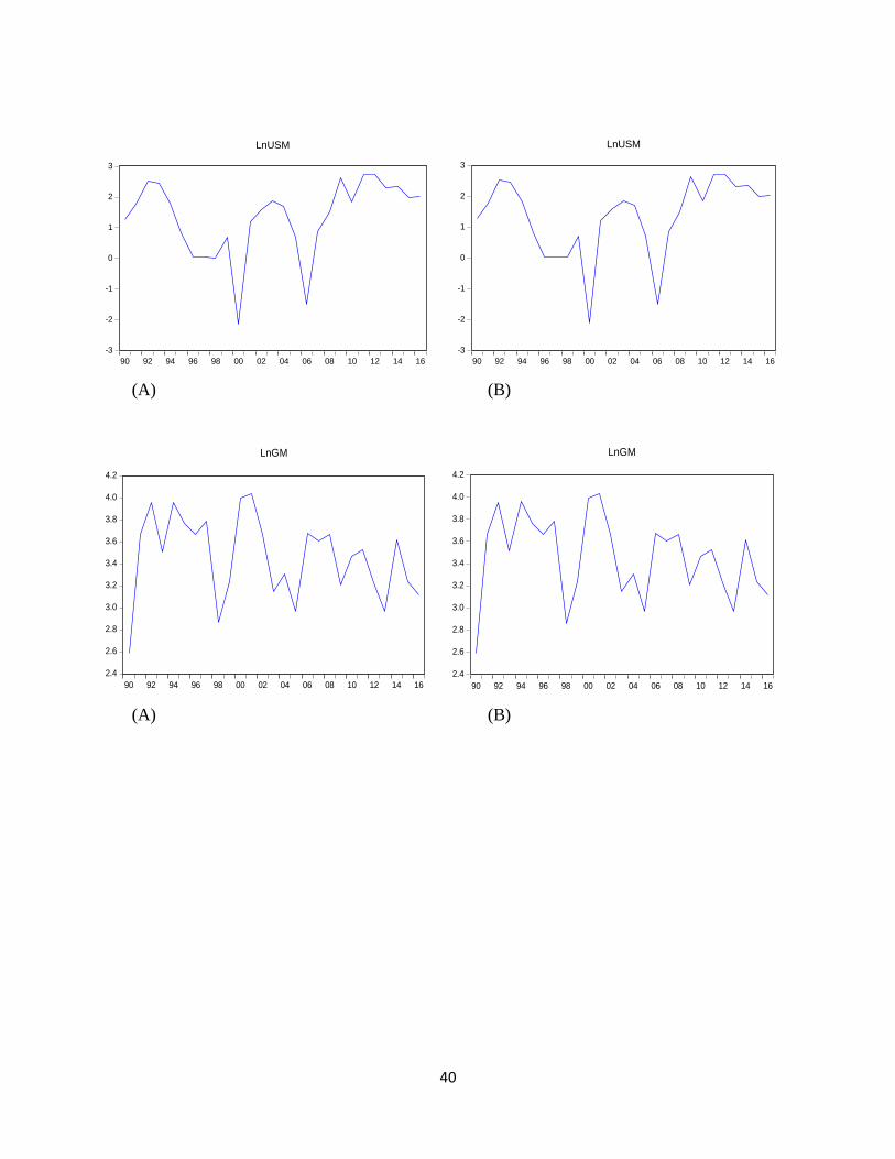
Appendix A.4
Graphs of Variables in First Differences
(A) (B)
(A) (B)
(A) (B)
-4
-3
-2
-1
0
1
2
90 92 94 96 98 00 02 04 06 08 10 12 14 16
LnER
-4
-3
-2
-1
0
1
2
90 92 94 96 98 00 02 04 06 08 10 12 14 16
LnER
10.0
12.5
15.0
17.5
20.0
22.5
25.0
27.5
30.0
90 92 94 96 98 00 02 04 06 08 10 12 14 16
GX
10.0
12.5
15.0
17.5
20.0
22.5
25.0
27.5
30.0
90 92 94 96 98 00 02 04 06 08 10 12 14 16
GX
0
5
10
15
20
25
30
35
40
90 92 94 96 98 00 02 04 06 08 10 12 14 16
RD
0
5
10
15
20
25
30
35
40
90 92 94 96 98 00 02 04 06 08 10 12 14 16
RD
40
(A) (B)
(A) (B)
-3
-2
-1
0
1
2
3
90 92 94 96 98 00 02 04 06 08 10 12 14 16
LnUSM
-3
-2
-1
0
1
2
3
90 92 94 96 98 00 02 04 06 08 10 12 14 16
LnUSM
2.4
2.6
2.8
3.0
3.2
3.4
3.6
3.8
4.0
4.2
90 92 94 96 98 00 02 04 06 08 10 12 14 16
LnGM
2.4
2.6
2.8
3.0
3.2
3.4
3.6
3.8
4.0
4.2
90 92 94 96 98 00 02 04 06 08 10 12 14 16
LnGM

41
VITA
Graduate School
Southern Illinois University Carbondale
Hilarious Edem Anku
University of Louisville, Kentucky
Bachelor of Science, Economics, May 2017
THESIS PAPER TITLE: SOURCES OF CURRENCY DEPRECIATION IN GHANA
MAJOR PROFESSOR: DR. AKM MAHBUB MORSHED