_ 1 _ Poverty trends since the transition Poverty trends since the transition

South African mega-events and their impact on

tourism

KARLY SPRONK AND JOHAN FOURIE

Stellenbosch Economic Working Papers: 03/10

KEYWORDS: SPORT, TOURIST ARRIVALS, WORLD CUP, DEVELOPING COUNTRIES

JEL: L83, F19

KARLY SPRONK DEPARTMENT OF ECONOMICS

UNIVERSITY OF STELLENBOSCH PRIVATE BAG X1, 7602

MATIELAND, SOUTH AFRICA E-MAIL: 14777231@SUN.AC.ZA

JOHAN FOURIE DEPARTMENT OF ECONOMICS

UNIVERSITY OF STELLENBOSCH PRIVATE BAG X1, 7602

MATIELAND, SOUTH AFRICA E-MAIL: JOHANF@SUN.AC.ZA

A WORKING PAPER OF THE DEPARTMENT OF ECONOMICS AND THE

BUREAU FOR ECONOMIC RESEARCH AT THE UNIVERSITY OF STELLENBOSCH

2

South African mega-events and their impact on

tourism 1

KARLY SPRONK2 AND JOHAN FOURIE3

ABSTRACT

The 2010 FIFA World Cup, one of the largest mega-sport events, has stirred

renewed interest in the benefits that a host country can derive from these events.

While most predict a large increase in the number of tourist arrivals, the recent

international literature suggest that ex ante studies are often too optimistic.

South Africa has played host to numerous mega-events since 1994. Using a time-

series auto-regressive model, we identify increases in tourism numbers for most

of these events, controlling for a number of variables standard in predicting

tourism flows. However, smaller events, especially those held during summer

months, show little increase in tourist arrivals. We disaggregate tourism arrivals

to show that, as expected, tourists from participating countries increase the most.

Contrary to the international literature, we find little evidence of displacement.

This could be as a result of off-season scheduling or because the relative size of

these events does not reflect that of the FIFA World Cup or Olympic Games.

Keywords: sport, tourist arrivals, World Cup, developing countries

JEL codes:L83, F19

1 The authors would like to thank Gideon du Rand, Le Roux Burrows, Krige Siebrits, Robert Baade, Markus Kurscheidt, Wolfgang Maennig and participants at the ‘Sport Mega events and their legacies’ conference held in Stellenbosch, South Africa in December 2009. 2 Department of Economics, Stellenbosch University 3 Department of Economics, Stellenbosch University. Corresponding author: johanf@sun.ac.za.

3

1. INTRODUCTION

The growth of the tourism industry in South Africa over the last two decades signal the country’s

ability to sustainably export travel services, improving the balance of payments, creating jobs and

boosting economic growth (Fourie 2010). The South African travel and tourism sector, of which

sport tourism is a subsection, will contribute 8.7% to Gross Domestic Product (GDP) in 2009

(WTTC 2009). One determinant of the rise in tourism is event tourism; tourists attracted to a

country or region with the specific aim of consuming event-specific goods. Mega-sport events, in

particular, are considered to entail significant benefits for the host country in terms of tourism

arrivals, both concurrently with the event and as a legacy (Baade and Matheson 2003; Baade and

Matheson 2004; Matheson and Baade 2004; Preuss 2004; Solberg and Preuss 2006; Preuss 2007;

Preuss 2007; Hagn and Maennig 2009).

South Africa has hosted major sporting events in the recent past, including the 1995 IRB Rugby

World Cup, 1996 African Cup of Nations, 2003 ICC Cricket World Cup, 2007 World Twenty20

Championships, 2009 Indian Premier League (IPL), 2009 British and Irish Lions tour, 2009

Confederations Cup and 2009 ICC Champions trophy. The success of hosting these events has

assisted South Africa in building its tourism infrastructure and has helped build its reputation as an

international tourist destination. Due to this, South Africa has won the bid to host the 2010 FIFA

Soccer World Cup, which has renewed interest in the benefits pertaining to mega-sport events.

There are numerous direct pecuniary and non-pecuniary benefits in hosting these events (Maennig

and Du Plessis 2007). For this paper, we focus on the impact of the change in tourist flows to South

Africa. We contribute to the international debate on mega-sport events, finding empirical evidence

to support our hypothesis that mega-events increase tourism arrivals, ceteris paribus. While this

seems an obvious conclusion, the recent literature suggest that mega-events do not necessarily

increase tourist numbers, as event-specific tourists may crowd-out or displace non-event tourists

(Solberg and Preuss 2006; Allmers and Maennig 2009; Preuss and Kurscheidt 2009). Reflecting on

five events held in South Africa since 1995, we find evidence to support both sides of the debate;

while some events do increase tourism, a few have no significant impact on tourism arrivals.

In order to understand the impact of sport events on the flow of tourists to South Africa it is

necessary to first address the confusion about the exact meaning of terms like sports, sport events

and tourists. This is addressed in Section 2. Section 3 follows with a discussion of the previous

studies conducted on the determinants of tourism inflows. A description of and motivation for the

data is provided in Section 4, with Section 5 covering data changes and limitations. The results from

are presented in Section 6 and Section 7 concludes.

2. SPORTS AND NON-SPORTS TOURISTS

Sport events can be defined as events that are characterised by creative and complex content of

sport-like, recreational activities, of entertaining character and are performed in accordance with a

particular predetermined programme. These events have an influence on tourism, which have great

4

social and economic significance for the location or region in which they are held (Bjelac and

Radovanovic 2003). Sport events vary in size and scope. Bjelac & Radovanovic (2003) categorize

events according to 7 different scales: “locally held events”, “regional or zonal events”, “national

sports events”, “national events with some international participation”, “continental competitions”,

“intercontinental events” and the largest known as “planetary events”. For the purpose of this paper

only the larger events with international participation are considered.

South Africa has played host to numerous sporting events but for the purpose of this paper only five

are considered. These events all took place at an international level and are classified as South

Africa’s three main major sport types: soccer (football), rugby and cricket. The five events chosen

for the paper are: the 1995 IRB Rugby World Cup, 2003 ICC Cricket World Cup, 2007 World

Twenty20 Cricket Championships, the British and Irish Lions rugby tour to South Africa and the

Indian Premier League (IPL), the last two events occurring in 2009. Because of data constraints on

African arrivals into South Africa, the African Cup of Nations held in South Africa in 1996 is not

included. Neither are the smaller events, like the Super 14 (previously Super12). Similarly the ABSA

Currie Cup is a national level rugby event and is ignored in this paper because events like these will

not have a significant effect on the volume of inbound tourists.

Events can also be characterised as primary, secondary or tertiary attractions. A primary attraction

has the power to influence a tourist’s decision to travel to South Africa. A secondary sport event or

tourist attraction is known to the tourists, but is not critical in the itinerary decisions (Hinch and

Higham 2004), while a tertiary attraction is not known to the tourists prior to their visit but is

experienced upon arrival at their destination (Higham 2005). Considering this distinction, it is

important to define the tourism element, as there is a difference between tourists travelling to

South Africa as non-event tourists or as sports tourists. A non-event tourist considers the sporting

event in the visited country as a secondary attraction while a sports tourist is defined as

“individuals and/or groups of people who actively or passively participate in competitive or

recreational sport, while travelling to and/ or staying in places outside their usual environment”

(Hinch and Higham 2004:19). The reason for the classification is because tourists often differ in

their consumption, and thus expenditure, of the services provided. However, because of the macro

nature of our study, we do not distinguish between the different classifications presented above.

We therefore assume all tourists equal, and use tourist arrivals as a proxy to measure the ‘gains’ to

the host nation. To the extent that sport tourists differ in their characteristics, length of stay and

expenditure patterns from non-sports tourists, however, the actual ‘gains’, i.e. in tourism

expenditure, could be different.

3. TOURISM AND DISPLACEMENT

Studies conducted on the topic of tourism determinants are numerous and in most cases, like

Solberg and Preuss (2006), do find that mega-events increase the number of arrivals of foreign

tourists to the host country. More recently, however, a number of authors are sceptical and regard

ex ante studies of mega-events as being too optimistic (Matheson 2002; Matheson and Baade 2004;

Matheson 2006; Preuss and Kurscheidt 2009). Maennig and co-authors (Allmers and Maennig

5

2009; Hagn and Maennig 2009), in particular, found that for the 2006 FIFA World Cup in Germany,

visitor numbers appear little different from the counterfactual of ‘normal’ tourism arrivals, even

though the 2006 World Cup is widely considered as one of the most successful yet. This has

important implications for countries that consider bidding for such an event, given the large

investments/expenditures required.

The critical issue with the increase in foreign arrivals (due to sporting events) is therefore the

problem of crowding-out or the displacement effect of normal tourists. In the 2010 FIFA World Cup

context, many authors are anxious about this (Preuss and Kurscheidt 2009), but the South African

sporting organisers have taken these fears into consideration and plan to limit the displacement of

normal tourists. They have done this by scheduling most of the large sporting events in the off

season, winter months when there are lower volumes of arrivals to host cities (Maennig and Du

Plessis 2007). As Higham (2005) points out with reference to the 2005 Lions tour in New Zealand,

this will curb displacement effects and may offer additional benefits to hosting large sports events

because there is now a demand in off-peak seasons.

This can be seen in practice with the IRB Rugby World Cup, British & Irish tour and the 2010 FIFA

Soccer World Cup which are held in the lowest arrival months of May and June (Figure 1), both

winter months in South Africa. On the other hand, the ICC Cricket World Cup and the World

Twenty20 Champions are summer sports. South Africa is typically seen as a summer destination by

tourists and the highest arrival months are therefore summers months. However both events were

scheduled for the lower tourist summer months of February and September. The IPL, another

variation of the game of cricket, was not scheduled for these low season summer months. This

scheduling problem was not due to bad planning from the South African organizers, but due to the

fact that the event’s location was shifted 3 weeks before the event was to commence, because of

security concerns in India.

While the timing of events is of high importance, it is nevertheless essential to consider the other

determinants of inbound tourism too. Previous research in this field has focused mainly on

developed countries and their explanation of tourist demand, while far less research has been

conducted for developing countries like South Africa. Early research methodologies used empirical

models of tourism demand based on consumer theory. This theory states that the optimal

consumption is influenced by the consumers’ income, the price of goods as well as the price of

substitutes and complementary goods. From this, a single equation model is determined to analyze

the tourist demand (Phakdisoth and Kim 2007).

Methodologies then advanced to time-series econometric models, focusing on the explanation of

tourist demand (Walsh 1996). More recently, a method used by Naudé and Saayman (2005) uses

panel data to determine demand and supply factor determinants. They found, specifically for Africa,

that political stability, tourism infrastructure, marketing and the stage of development are key

aspects in explaining tourism demand. Similarly, Saayman and Saayman (2008) find that, apart

from the standard demand-side variables, climate (with the number of sunny days in Cape Town

used as proxy) also attracts visitors. Fourie, du Toit and Trew (2010) extend Zhang and Jensen’s

6

(2007) supply-side analysis of the determinants of tourism and find evidence that the natural

environment is an important predictor of a country’s tourism comparative advantage, while

neighbouring countries and a country’s relative transport infrastructure are also determinants of

tourism. This is especially true of sub-Saharan Africa (Fourie 2009).

The research data of tourism demand models have established that travel costs are an important

determinant in the flow of inbound tourism. These costs are an important component of a tourist’s

decision to visit a place, or not and are especially important because the majority of South Africa’s

international tourist utilise air transport. The passenger air transport industry was established in

the 1950’s, but was only affordable to the rich. The improvement and development of factors like

technology and communications as well as rising levels of income, the opening of international

borders and economic growth of the major industrialised countries (Ringbeck, Gautam et al. 2009),

have made travelling more affordable to the masses.

This has stimulated the trade and travel industry and presented more opportunities for sport

tourism to flourish (Gibson 1998). The fear, however, of some countries, like South Africa, is the

influence that oil prices have on travel costs (Ringbeck, Gautam et al. 2009). A steep increase in oil

prices will negatively impact the volume of arrivals, especially from distant developed countries

that make use of long-haul flights to reach destinations, resulting in a dampening of the growth of

the travel and tourism sector.

Yet there are few attempts to measure the impact of mega-events on South African tourism

indicators. South Africa’s successful bid to host the FIFA World Cup in 2010 has garnered greater

interest in the field, although these ex ante studies are riddled with strong assumptions based on

developed country studies. In the only attempt to measure the impact of mega-events on tourist

arrivals using a gravity equation approach, Fourie and Santana-Gallego (2010) find evidence to

support the notion that mega-events create ‘additional’ tourism arrivals ceteris paribus. However,

their results show startling differences in outcome depending on the type of event, the income per

capita of the host country, and the timing of the event. They find a significantly positive impact of

8% on tourist arrivals to South Africa, for example, of hosting the 2003 Cricket World Cup (Fourie

and Santana-Gallego 2010). While reports and press articles have often appeared after an event to

cite the benefits to the South African economy of hosting such an event (Magubane 2009), none of

these consider the counterfactual impact on tourism. This study is therefore an attempt to measure

the increase in tourism when hosting a mega-event, controlling for various explanatory factors.

4. DATA DESCRIPTION

To establish the effects that a sporting event has on the normal inbound number of tourists to South

Africa, an assessment of the changes in tourists to South Africa are calculated. This is done for each

sporting event and each country’s arrivals. To make an accurate assessment of the arrivals, other

variables that would influence the decisions of tourists to visit South Africa are calculated. The

model used in this paper is based on the findings of Sinclair (1998) that foreign tourist arrivals are

a function of income of the originating country, relative prices, and transportation costs between

7

the two destinations.

4.1. Data description of arrivals

Measuring the change of tourist arrivals means that the dependent variable is foreign inbound

tourism in a country. The inbound volume can be determined by one of two different methods,

either by using the expenditure and receipts of tourists, or by the volume of tourist arrivals in South

Africa. Tourist arrivals is a readily available statistic, while there is no consistency (Saayman &

Saayman,2008: 84) in the data collected for expenditure by and receipts from tourists in South

Africa. For this reason, this paper uses foreign tourist arrivals ranging from January 1983 to July

2009.

Statistics South Africa (StatsSA) collects monthly data for foreign arrivals from the various

countries, published in Tourism and Migration (P0351). Foreign visitors are defined as being any

travelers who are not South African citizens or permanent residents. For the purpose of this paper,

only the following countries air arrivals are included: Australia, France, Germany, India,

Netherlands, New Zealand, United Kingdom (UK) and the United States of America (USA). It is

assumed that transfers are zero for incoming arrivals during the period of the event.

African arrivals are completely neglected from the arrivals data although African arrivals contribute

largely to the total volume of arrivals in South Africa. This aspect is problematic because South

Africa totally encloses Lesotho and Swaziland. Tourists from other parts of Africa, specifically from

these two countries, travel to South Africa for different reasons to those of foreign tourists

(Saayman and Saayman 2008). Foreign international tourists are also considered to be bigger

spenders and have a greater effect on the economic benefit and importance of travel and tourism

sector to the South African economy (Saayman and Saayman 2008).

The African arrivals are included in the total arrivals to South Africa in Figure 1. In comparison to

Figure 2 (especially Germany, UK and France) there seems to be no clearly visible trend in Figure 1.

The red mean line for each month shows that tourists favour South African summer months as a

holiday destination (January and December). On the other hand the winter months of May and June

have a lower mean volume of arrivals. This seems intuitive as the primary market (Western

Europe) is situated in the Northern hemisphere. We can see that for the combined data (which

includes Southern hemisphere and other African countries), this effect is watered down.

8

Figure 1: Total international tourist arrivals per month with mean values (Jan 1983-July 2009)

The identified primary markets travelling to South Africa as tourists are: Germany, Netherlands,

France and the UK. Explanations for identifying these as primary markets come from cultural and

colonial ties. It is important to try and recognise any negative effects that hosting large sporting

events can have on the primary market, which largely supports the South African tourism sector.

However, it is also vitally important to acknowledge the effect that these events have on attracting

fans (tourists) from countries that participate in the events. This is based on the understanding that

the fans (tourists) would not otherwise have travelled to South Africa if it were not for the sporting

event. Indian arrivals are included because it accounts for the IPL, ICC Cricket World Cup and the

ICC World Twenty20. The UK is already identified as a primary market but is also included because

of their participation in the ICC Cricket World, ICC World Twenty20, IRB Rugby World Cup and the

British and Irish Lions tour. Australia and New Zealand are included because both countries

participated in the ICC World Twenty20, ICC Cricket World Cup and IRB Rugby World Cup

participation. While the USA is not a participant in any of the sporting events identified in this

paper, it is included as the arrivals from the USA to South Africa are relative large.

Figure 2 is once again a seasonal representation (similar to Figure 1) of the tourist arrivals to South

Africa, but is shown per country. The Northern hemisphere countries of the Western Europe

(France, Germany, Netherlands and UK) all follow the same trend as described above, with the USA

the exception. This could be explained by the USA’s weather diversity (e.g. East and West coasts

experience very different weather patterns during the same season). Thus they may travel to South

Africa for reasons other than Europeans. New Zealand and Australia do not follow a strict arrival

trend associated with weather conditions because the seasons of both countries correspond to the

South African seasons as they are both situated far south in the Southern hemisphere.

0

200,000

400,000

600,000

800,000

1,000,000

1,200,000

Jan Feb Mar Apr May Jun Jul Aug Sep Oct Nov Dec

Total international tourist arrivals per month with mean values (Jan 1983 - July 2009)

9

4.2. Description of data for the income of originating country

Income of the respective originating countries refers to the GDP of the country in question. For

India this variable was the GDP at purchasing power parity. The data is obtained from the

International Monetary Fund’s World Economic Outlook. The Indian GDP is measured annually in

billions of US dollars (current international dollar) for the period. There is, however, a mismatch of

frequencies concerning the other data used in the model and the GDP. The data is therefore linearly

interpolated using Stata 9 to convert the quarterly series into monthly data.

The GDP for the remainder of the countries (UK, Australia, France, Germany, Netherlands, New

Zealand and USA) is expressed in the national currency for every quarter. This data is also linearly

interpolated using the same method as above, to convert it from a quarterly to a monthly form to be

compatible with the rest of the existing data. It is also converted from a nominal to real series. For

these real figures to be calculated it is necessary to use the GDP deflators (all 2005 = 100) for each

of the countries in question. The deflators are obtained from the International Monetary Fund’s

International Financial Statistics.

10

Figure 2: International tourist arrivals per country with monthly mean average (Jan 1983 – July 2009)

0

2,000

4,000

6,000

8,000

10,000

12,000

Jan Feb Mar Apr May Jun Jul Aug Sep Oct Nov Dec

India

0

400

800

1,200

1,600

2,000

2,400

2,800

Jan Feb Mar Apr May Jun Jul Aug Sep Oct Nov Dec

New Zealand

0

10,000

20,000

30,000

40,000

Jan Feb Mar Apr May Jun Jul Aug Sep Oct Nov Dec

Germany

0

10,000

20,000

30,000

40,000

Jan Feb Mar Apr May Jun Jul Aug Sep Oct Nov Dec

United States of America

11

Figure 2: International tourist arrivals per country with monthly mean average (Jan 1983 – July 2009)

0

2,000

4,000

6,000

8,000

10,000

12,000

Jan Feb Mar Apr May Jun Jul Aug Sep Oct Nov Dec

Australia

0

4,000

8,000

12,000

16,000

20,000

Jan Feb Mar Apr May Jun Jul Aug Sep Oct Nov Dec

France

0

5,000

10,000

15,000

20,000

25,000

Jan Feb Mar Apr May Jun Jul Aug Sep Oct Nov Dec

Netherlands

0

10,000

20,000

30,000

40,000

50,000

60,000

70,000

Jan Feb Mar Apr May Jun Jul Aug Sep Oct Nov Dec

United Kingdom

12

4.3. Description of data for the relative prices

Decisions about prices in the destination relative to the prices in the country of origin are a large

determining factor of tourist flows. If prices in the country of destination are cheaper than the

country of origin then the tourist’s currency is worth more in the country they are visiting. This

should be reflected with an increase in the volume of arrivals to the destination.

To accurately measure the relative price variable a proxy must be used. The exchange rate of the

South African Rand (Rand) is used as a proxy instead of relative price indices. The exchange rate is

expressed in the Rand per foreign currency denomination. The exchange rate is expressed for the

Australian Dollar, Indian Rupee, USA Dollar ($), British Pound (£), New Zealand Dollar and the

European Union (€) (which includes France, Germany, Netherlands) Euro.

The exchange rate of rand per US $, rand per £ and rand per € are sourced from the RSA Reserve

Bank’s (SARB) monthly data release and is an average of the daily averages of each rate. The Indian

Rupee, Australian dollar and New Zealand dollar are expressed as AUS $ per US $, NZ $ per US $ and

Rupee per US $ respectively at a market rate for the monthly average, with the Rand denoted at a

principal rate. All the exchange rates were adapted from the International Monetary Fund’s

International Financial Statistics. The Australian, New Zealand and Indian exchange rates

conversions to the rand are calculated by dividing the foreign currency per US $ by the Rand per US

$.

Once the above mentioned conversions are done, all the currencies are nominal Rand denominated

exchange rates (NER). With all currencies expressed this way, it is easy to convert to a real

exchange rate. A real exchange rate is calculated to control the difference in inflation between South

Africa and the country of origin. The conversion to real exchange rate (RER) is calculated by

multiplying the CPI of the origin country over South African CPI;

The Consumer Price Index (CPI) data is obtained from the International Monetary Fund’s

International Financial Statistics and the Australian and New Zealand data are sourced from the

OECD financial indicators. The CPI time series data for Germany does not date back to January 1983

because of different time-series for West and East Germany. The time period for Germany is thus

limited to the period after unification, January 1991 to June 2009.

4.4. Description of data for travel costs

Finally, travel costs must be determined. The transport cost involved in transporting a supporter

(tourist) to the destination or host country influences the costs. This is especially relevant for South

Africa where the primary markets usually use long-haul flights. A proxy of dollar price of Brent

crude oil per barrel is used as proxy for travel costs. Crude oil per barrel is used instead of jet fuel,

as suggested by Saayman and Saayman (2008). The oil price data is obtained from the South African

Reserve Bank and is available in monthly format from January 1981 to the most recent data of June

2009.

13

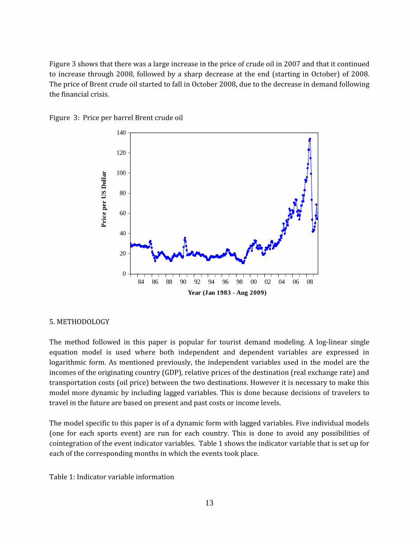
Figure 3 shows that there was a large increase in the price of crude oil in 2007 and that it continued

to increase through 2008, followed by a sharp decrease at the end (starting in October) of 2008.

The price of Brent crude oil started to fall in October 2008, due to the decrease in demand following

the financial crisis.

Figure 3: Price per barrel Brent crude oil

5. METHODOLOGY

The method followed in this paper is popular for tourist demand modeling. A log-linear single

equation model is used where both independent and dependent variables are expressed in

logarithmic form. As mentioned previously, the independent variables used in the model are the

incomes of the originating country (GDP), relative prices of the destination (real exchange rate) and

transportation costs (oil price) between the two destinations. However it is necessary to make this

model more dynamic by including lagged variables. This is done because decisions of travelers to

travel in the future are based on present and past costs or income levels.

The model specific to this paper is of a dynamic form with lagged variables. Five individual models

(one for each sports event) are run for each country. This is done to avoid any possibilities of

cointegration of the event indicator variables. Table 1 shows the indicator variable that is set up for

each of the corresponding months in which the events took place.

Table 1: Indicator variable information

0

20

40

60

80

100

120

140

84 86 88 90 92 94 96 98 00 02 04 06 08

Price per barrel brent crude oil

Pric

e p

er U

S D

oll

ar

Year (Jan 1983 - Aug 2009)

14

Sporting events Date Dummy variable month

IRB Rugby World Cup 25 May – 24 June 1995 May, June ICC Cricket World Cup 9 February – 24 March 2003 February, March ICC World Twenty20 11 September – 24 September 2007 September Indian Premier League 18 April – 24 May 2009 May British and Irish rugby tour 25 May – 24 June 2009 June

It is the coefficients of these indicator variables that we are particularly interested in to show the

increased effect of inbound tourists to South Africa. It is however important to consider the

significance of these coefficients of the indicator variables for each country’s arrivals. A dynamic

specification of the model (auto regressive model) is as follows:

The dependent variable for the dynamic model is the logarithmic of , the volume of tourist arrivals

of country . It is important to note because of auto-correlation in the dependent variable, as the

correlogram (calculated using Eviews 6) of table 8 in the appendix demonstrates. To resolve this,

the model has to be more dynamic by including lags of the dependent variable. This model is known

as an autoregressive model of the process order p with p the number of lags. Each country’s lagged

periods of the dependent variable (arrivals) are determined individually.

The summation of is the general form that captures the vector of the logarithmic variables

controlled for, including the lags (j) possible for the entire period (p). The vector represents the

tourist arrivals data as well as oil prices, GDP and real exchange rate of country . A model for each

country is developed. This is done because countries included in this paper differ greatly with

regard to the variables. With individually tailored models the data for each country is captured,

resulting in better models that fit the data. The variable time is the time indicator variable, and the z

variable is the event-specific indicator variable (sporting event) for the particular month. The q

vector variable is an indicator of the months and is included to account for seasonality trends.

These variables are the same for all models. The variable is the error term variable that is

homoskedastic with a zero mean.

Before an individual model is designed for each country, a vector autoregression estimate is run to

provide a basis from which the lag lengths of the dependent and independent variable can be

determined, so as to avoid serial correlation. The first order serial correlation is identified by the

Durbin-Watson static. It revealed that serial correlation exists; these estimates of the coefficients

are biased and inconsistent. The Durbin-Watson statistic measures the linear relationship between

adjacent residuals from a regression. With the aid of the results from the Durbin Watson statics and

the vector auto regressive estimates as a basis, more accurate models can be developed. The results

from the vector auto regression suggest the lag length of the variables for different periods, each

15

period is defined as a month. These results are available in the appendix table 9-16 and the

suggested lagged periods are highlighted in each case and are all significant at a 90% confidence

interval.

The development of the best model for individual countries is calculated from numerous estimates

of models, set up using E-views 6. The best model is thus achieved by a comparison of the models

because each variable can be lagged for all the suggested periods or different combination of the

periods, depending on the criterion statistics of the models that are compared. The most fitted

model was strongly influenced by the results obtained from the Akaike information criterion and

Schwarz criterion.

6. RESULTS FROM MODEL SPECIFICATION

The best suited model for each country is calculated according to the methodology described and

this includes the accurate lagged variables. The exact numbers of lags of each variable for the

various models is included in the appendix (Table 17).

The models are then regressed with the 5 different event specific indicators (as mentioned in Table

1) for the 8 different countries. The results are provided below. The period used in these

regressions (shaded bars) for all but Germany, is January 1984 till June 2009. As a result of

Germany’s divided statistics (between East and West Germany), the German models are limited and

the harmonised data on Germany only commences from mid-1994.

A shortcoming in the model estimates exists in that there is no indicator that captures the effect of

social/political instability or health epidemics linked to travelling such as the terrorist attacks on

the World Trade Centre in 2001, the SARS epidemic or most recently the health epidemic of Swine

flu. These problems not only affect the citizens of the country but the decisions of all the

international travelers. For these reasons and to support the results obtained by the initial models

(shaded bars) a test of the robustness of these results is undertaken. The same model is run over

different time spans. For the 1995 Rugby World Cup, only six years of data is available before the

event occurs, and the window thus captures the changes that took place between January 1989 and

June 2009. Similarly the second window is limited from the beginning of 1995 to June 2009. The

German models are excluded from the 1995 estimates as the model cannot be regressed, due to

insufficient data for the period. For the 2003 ICC Cricket World Cup the second window is altered

somewhat and an additional third window is included. The second window runs from January 1999

to June 2009 while the third runs from January 2003 to June 2009. The last three events

(Twenty20, IPL, Lions Tour) all use the same three windows; January 1989 to June 2009, January

1999 to June 2009 and January 2005 to June 2009.

6.1 IRB Rugby World Cup 1995 estimates

The 1995 Rugby World Cup was the first international sporting event to be hosted by the Republic

of South Africa following the fall of Apartheid. The 1995 Cup was the third occasion of this

16

competition and a first time appearance for the Springboks after their re-admittance in 1992. This

event attracted a lot of international media attention, not only because of the sheer size of the

Rugby World Cup but because the unique political events that preceded the tournament.

This event drew many spectators and inquisitive visitors alike to experience the South African

version of the World Cup, and, compared to the counterfactual of not hosting the World Cup, overall

arrivals increased significantly. Sixteen countries took part in the event. Following on Table 2, the

participating countries used in this paper are highlighted in bold: Australia, France, New Zealand

and England (UK). The coefficients (µ) of the event specific indicator for these countries are all

statistically significant at a 5% level of significance. The significance level of 5% is used throughout

the paper to test statistical significance of the estimates.

The tourists from Australia to South Africa increased by approximately 54%, ceteris paribus, for the

months that the Cup was hosted. The robustness checks provide evidence that this result is robust.

The first window shows arrivals increased by approximately 58%, ceteris paribus. The second

window starts at the beginning of 1995 and therefore does not capture the historically low levels of

arrivals experienced in South Africa during the Apartheid era. The second window compares future

arrivals with arrivals from this event; therefore the effect seems to be reduced. However, even

though the absolute value of the change of arrivals is affected it is still a notably significant increase

in arrivals of 29%.

New Zealand and Australia are two of the biggest rugby playing nations in the southern

hemisphere. This is reflected in the absolute change in arrivals from these two countries, although

the increases from France and UK are large and significant too. Tourists from New Zealand

increased by 112%, ceteris paribus, for the months that the Cup was hosted. This is a reflection that

arrivals from this country are very low and increased significantly because of the World Cup. The

robustness checks provide further evidence that this figure is correct. The first and second window

show arrivals increase by approximately 117% and 108% respectively, ceteris paribus.

Tourists from France and the United Kingdom follow a similar trend as the Australian arrivals. The

French and British arrivals increased by 48% and 33% respectively, ceteris paribus, for the months

that the Cup was hosted. Both changes are statistically significant at 5% level of significance and the

checks give evidence that this is robust. The first window shows arrivals increased by

approximately 47% and 37% respectively. The third window, using only the post-1994 period, still

finds a notably large increase in arrivals of 27% for both countries. For the remainder of the

countries not participating, there are no statistically significant changes in arrivals noted because of

the event. It is interesting to note that a decrease is observed in the third window of these

countries, but these changes are not statistically significant and are therefore not clear evidence of

cross-country displacement.

17

Table 2: Results of Rugby World Cup estimates

Country Change(%) of arrivals Size of µ Std. error T- statistic

Australia* 54.25 0.5425 0.1409 3.8516

1989/01 - 2009/06 57.69 0.5769 0.1240 4.6505

1995/01 - 2009/06 28.78 0.2878 0.1130 2.5469

France* 48.15 0.4815 0.1410 3.4152

1989/01 - 2009/06 47.45 0.4745 0.1383 3.4318

1995/01 - 2009/06 26.86 0.2686 0.1171 2.2938

Germany Not sufficient data

India* 11.96 0.1196 0.1721 0.6950

1989/01 - 2009/06 15.24 0.1524 0.1364 1.1172

1995/01 - 2009/06 -5.20 -0.0520 0.1237 -0.4203

Netherlands 13.41 0.1341 0.1800 0.7449

1989/01 - 2009/06 13.75 0.1375 0.1802 0.7631

1995/01 - 2009/06 -11.52 -0.1152 0.1805 -0.6382

New Zealand* 111.59 1.1159 0.1582 7.0526

1989/01 - 2009/06 116.68 1.1668 0.1486 7.8525

1995/01 - 2009/06 107.57 1.0757 0.1290 8.3413

UK* 33.20 0.3320 0.1270 2.6150

1989/01 - 2009/06 37.15 0.3715 0.1142 3.2527

1995/01 - 2009/06 26.62 0.2662 0.1157 2.3003

USA 5.81 0.0581 0.1074 0.5414

1989/01 - 2009/06 1.83 0.0183 0.1029 0.1775

1995/01 - 2009/06 -14.28 -0.1428 0.1094 -1.3058

6.2 ICC Cricket World Cup 2003 estimates

The 2003 ICC Cricket World Cup, hosted by South Africa (including a few matches in Zimbabwe and

Kenya) was the first time this competition was held on African soil and the eighth of its kind.

Fourteen countries took part in the event. Table 3 lists the participating countries used in this paper

and are highlighted in bold; Australia, India, Netherlands, New Zealand and England (UK).

Although tourists from Australia, Netherlands and UK increased, this increase is not statistically

significant at the 5% level. This means that the event did not attract more tourists than would have

travelled to South Africa under normal circumstances. The New Zealand arrivals shows a 64%

increase, ceteris paribus. The robustness checks of this change shows that they contradict the initial

change, however, and none of the checks are statistically significant. Therefore it can be inferred

that arrivals did increase during the tournament, but perhaps not at such a high rate as the initial

change first suggested.

18

Cricket is a national sport in India with a massive supporter base. The results obtained for the

World Cup is thus unsurprising. The initial change shows an increase of approximately 64%, ceteris

paribus, for tourists from India for the months that the Cup was hosted. The robustness checks

support this. The first, second and third window all show arrivals increase by approximately 64%,

69% and 65% respectively, ceteris paribus, and these are all statistically significant. This is a

reflection that arrivals from these countries are on average very low and increased dramatically

during the months of the World Cup.

For the remainder of the countries not participating, there is no statistically significant change in

arrivals noted because of the event. A notable decrease is observed for arrivals from the United

States during the tournament but these changes are not statistically significant at a level of 5%.

Table 3: Results of Cricket World Cup estimates

Country Change(%) of arrivals Size of µ Std. error T- statistic

Australia 10.54 0.1054 0.1442 0.7313

1989/01 - 2009/06 6.58 0.065847 0.13021 0.5057

1999/01 - 2009/06 11.39 0.113899 0.058433 1.949237

2003/01- 2009/06 11.35 0.113512 0.06385 1.777805

France 17.38 0.1738 0.1434 1.2115

1989/01 - 2009/06 15.61 0.156129 0.142505 1.095603

1999/01 - 2009/06 7.43 0.074346 0.072918 1.01959

2003/01- 2009/06 4.21 0.042083 0.088263 0.476789

Germany 11.76 0.1176 0.1189 0.9892

1995/08 - 2009/06 11.76 0.117599 0.118889 0.989154

2003/01- 2009/06 -5.93 -0.0593 0.061411 -0.965605

India* 64.18 0.6418 0.1776 3.6150

1989/01 - 2009/06 64.11 0.641061 0.140647 4.557954

1999/01 - 2009/06 68.91 0.689134 0.104835 6.573527

2003/01- 2009/06 64.97 0.649737 0.12759 5.092383

Netherlands 6.41 0.0641 0.1839 0.3487

1989/01 - 2009/06 5.17 0.051704 0.185488 0.278745

1999/01 - 2009/06 4.24 0.042398 0.090373 0.469137

2003/01- 2009/06 2.42 0.024167 0.07245 0.333574

New Zealand* 64.18 0.6418 0.1776 3.6150

1989/01 - 2009/06 -1.28 -0.01281 0.162502 -0.078823

1999/01 - 2009/06 13.16 0.131596 0.081558 1.613526

2003/01- 2009/06 9.37 0.093704 0.086188 1.087196

UK 5.32 0.0532 0.1299 0.4096

1989/01 - 2009/06 4.23 0.042337 0.118845 0.356238

1999/01 - 2009/06 -3.64 -0.03641 0.070917 -0.513431

19

2003/01- 2009/06 -9.31 -0.09305 0.083033 -1.120648

USA -2.74 -0.0274 0.1068 -0.2570

1989/01 - 2009/06 -1.32 -0.01318 0.101355 -0.130033

1999/01 - 2009/06 -6.93 -0.06933 0.056598 -1.224996

2003/01- 2009/06 -7.04 -0.07044 0.056382 -1.249413

6.3 ICC World Twenty20 2007 estimates

South Africa was the first country to host the inaugural Twenty20 World Championships. Twelve

teams participated in a thirteen day event. Table 4 lists the participating countries used in this

paper and are highlighted in bold: Australia, India, New Zealand and England (UK). Although the

event itself was a marvellous success according to the organisers, it is not well reflected in the

results obtained which are statistically poor. The poor results could be attributed to the small size

of the event or the fact that it is an inaugural event which did not attract many tourists to South

Africa during the period.

For the remainder of the countries not participating, France, Germany, Netherlands and the USA

there are no statistically significant changes in arrivals noted because of the event. The robustness

check results are sporadic and form no noteworthy trend to report on. The USA however shows an

approximate band of decrease in the initial and robust checks. This could be linked to the housing

bubble which burst in 2007 but would not have yet affected the GDP and is therefore not controlled

for in the estimates. This is mainly speculative as these findings are not statistically significant.

Table 4: Results of Cricket Twenty20 estimates

Country Change(%) of arrivals Size of µ Std. error T- statistic

Australia -0.27 -0.002695 0.202636 -0.013301

1989/01- 2009/06 0.41 0.004130 0.180779 0.022845

1999/01- 2009/06 -0.50 -0.005039 0.079659 -0.063256

2005/01- 2009/06 2.57 0.025749 0.092164 0.279385

France -13.32 -0.133186 0.199995 -0.665946

1989/01- 2009/06 -16.80 -0.167977 0.196905 -0.853086

1999/01- 2009/06 -18.26 -0.182594 0.098663 -1.850694

2005/01- 2009/06 -0.91 -0.009112 0.072258 -0.126102

Germany -2.20 -0.022025 0.162457 -0.135572

1999/01- 2009/06 -3.81 -0.038129 0.095364 -0.399824

2005/01- 2009/06 -0.16 -0.001557 0.092488 -0.016834

India -10.83 -0.108266 0.244354 -0.443070

1989/01- 2009/06 -9.51 -0.095079 0.193296 -0.491885

1999/01- 2009/06 -13.58 -0.135834 0.151696 -0.895434

2005/01- 2009/06 -13.45 -0.134471 0.159921 -0.840861

20

Netherlands 7.43 0.074285 0.255504 0.290741

1989/01- 2009/06 2.94 0.029384 0.256003 0.114780

1999/01- 2009/06 -13.36 -0.133632 0.121063 -1.103827

2005/01- 2009/06 -0.97 -0.009742 0.104583 -0.093155

New Zealand 14.00 0.140034 0.238101 0.588130

1989/01- 2009/06 16.63 0.166265 0.230786 0.720431

1999/01- 2009/06 9.19 0.091934 0.117537 0.782167

2005/01- 2009/06 14.67 0.146713 0.135192 1.085215

UK -2.52 -0.025193 0.178395 -0.141220

1989/01- 2009/06 -6.46 -0.064618 0.160333 -0.403023

1999/01- 2009/06 -4.58 -0.045788 0.090663 -0.505038

2005/01- 2009/06 -4.40 -0.043960 0.133495 -0.329302

USA -13.31 -0.133141 0.150495 -0.884686

1989/01- 2009/06 -12.12 -0.121160 0.142085 -0.852728

1999/01- 2009/06 -12.89 -0.128882 0.077978 -1.652804

2005/01- 2009/06 -12.99 -0.129917 0.094356 -1.376883

6.4 Indian Premier League (IPL) 2009 estimates

Three weeks before the second season of the Indian Premier League, an event that was originally

set to be held annually in India, the event was moved to South Africa. Unlike previous events this

event did not have participants from different countries but instead eight different franchise teams.

The franchises are owned mainly by wealthy Indians that pay large sums to contract top

international and domestic Indian cricket players.

The IPL should therefore only largely affect the tourists coming from India to South Africa, as is

reflected in Table 5, with the India results highlighted in bold. There is a large increase of arrivals

from India of approximately 60%, ceteris paribus, for the months that the IPL was hosted. The

robustness checks give evidence that this figure is more or less correct. The first, second and third

windows all show arrivals increased by approximately 43% , 56% and 61%, respectively, ceteris

paribus, and these are all statistically significant. This is a reflection that arrivals from this country

are on average low, but because of the IPL event, the increase was substantial.

For the remainder of the countries not participating, there are no statistically significant changes in

arrivals found because of the event. Except for the United Kingdom’s arrivals, the initial change

because of the event is a decrease of 29%, but which is not statistically significant. The first window

renders a decrease of 22% (also statistically insignificant); however, the second and third maintain

the decreasing trend and was statistically significant. Although possibly a case of displacement, the

type of displacement is not clear; British travellers may have shifted their arrival in South Africa to

coincide with the British and Irish Lions rugby tour that occurred one month later. Rather than the

Indian Premier League displacing tourists from Britain, the negative coefficient may simply be as a

result of shifting expenditures to accommodate the Lions tour.

21

Furthermore, Fourie, Siebrits and Spronk (2010) argue that the IPL and Lions tour provide a unique

natural experiment to measure the size of displacement. Because of the sudden shift in the IPL

event, expected displacement would be small given the short notice and the fact that most tourists

book their visits well in advance. In contrast, the Lions tour was scheduled two years and advance

and tourists would have had enough time to shift their expenditure (i.e. for British rugby

enthusiasts to displace non-event tourists). Fourie et al. (2010) find some evidence of displacement,

although this is relatively small compared to the additional tourism gains.

Table 5: Results of IPL estimates

Country Change(%) of arrivals Size of µ Std. error T- statistic

Australia -5.35 -0.0535 0.2190 -0.2442

1989/01- 2009/06 -8.11 -0.081129 0.196386 -0.41311

1999/01- 2009/06 -6.51 -0.065091 0.088583 -0.734806

2005/01- 2009/06 -7.41 -0.07409 0.093152 -0.795362

France -7.25 -0.0725 0.2098 -0.3454

1989/01- 2009/06 -2.22 -0.022212 0.210515 -0.105514

1999/01- 2009/06 1.32 0.013178 0.109806 0.120014

2005/01- 2009/06 5.62 0.056184 0.070558 0.796284

Germany -17.54 -0.1754 0.1766 -0.9934

1999/01- 2009/06 -17.44 -0.174361 0.102454 -1.701843

2005/01- 2009/06 1.90 0.019008 0.092703 0.205037

India* 59.68 0.5968 0.2508 2.3798

1989/01- 2009/06 43.39 0.433857 0.200157 2.167582

1999/01- 2009/06 55.55 0.555468 0.154129 3.603923

2005/01- 2009/06 60.85 0.60854 0.121491 5.008941

Netherlands 6.11 0.0611 0.2681 0.2279

1989/01- 2009/06 0.28 0.002814 0.271189 0.010375

1999/01- 2009/06 -2.16 -0.021611 0.130276 -0.165884

2005/01- 2009/06 12.00 0.120019 0.107401 1.117485

New Zealand -11.30 -0.1130 0.2457 -0.4598

1989/01- 2009/06 -5.03 -0.050278 0.239388 -0.210027

1999/01- 2009/06 11.01 0.110096 0.122807 0.896495

2005/01- 2009/06 21.89 0.218892 0.132807 1.648201

UK -28.63 -0.2863 0.1877 -1.5248

1989/01- 2009/06 -22.46 -0.224618 0.175015 -1.283425

1999/01- 2009/06 -37.89 -0.378902 0.096199 -3.938739

2005/01- 2009/06 -43.51 -0.43506 0.112043 -3.882966

22

USA 1.66 0.0166 0.1578 0.1051

1989/01- 2009/06 2.03 0.020256 0.151236 0.133939

1999/01- 2009/06 2.10 0.020987 0.083553 0.251182

2005/01- 2009/06 5.03 0.050287 0.082667 0.608311

6.5 British & Irish Lions Rugby Tour 2009

The 2009 British and Irish Lions union tours have become a tradition which occurs every four years

between the three rugby power houses of the southern hemisphere: Australia, New Zealand and

South Africa and a combined team from the three home unions of Britain (England, Scotland and

Wales) and Ireland. It is important to note that the FIFA 2009 Confederations Cup took place in

South Africa during the end of the Lions tour. The Lions tour influenced arrivals primarily

originating from the UK, while the Confederations Cup had 8 teams participating of which New

Zealand and the USA are included in this paper. Fortunately, the English soccer team did not

participate and as such our results should not suffer from biased estimates.

It is assumed that all the supporters of the Lions tour will originate from the countries that the

players are selected from. Therefore the results of tourists coming from United Kingdom to South

Africa are highlighted in bold in Table 6. There is a large increase of arrivals of approximately 57%,

ceteris paribus, for the month that the tour was hosted by South Africa. The robustness checks of

this figure provide further support. The first, second and third windows show arrivals increase by

approximately 78%, 70% and 68%, respectively, ceteris paribus, and these are all statistically

significant. Given that Britain is a leading tourism market for South Africa, a large and significant

increase suggests that the Lions tour is an extremely lucrative competition to host.

For the remainder of the countries not participating, there are no statistically significant changes in

arrivals noted because of the event, except for the Indian arrivals, where a decrease of 54%, ceteris

paribus, is found. The first, second and third windows shows arrivals decrease by approximately

65%, 46% and 60%, respectively. This is almost a mirror image of the large increase which

occurred the month before, when the IPL tournament was hosted. While the model should capture

the expected decrease after the event with the lagged dependent variable, the change is so dramatic

that the decrease is still significant. This may provide some evidence that Indians shifted their

planned visits during June/July to May to coincide with the IPL event.

Table 6: Results of Lions tour estimates

Country Change(%) of arrivals Size of µ Std. error T- statistic

Australia 50.67 0.5067 0.4400 1.1515

1989/01- 2009/06 61.09 0.610948 0.425733 1.435049

1999/01- 2009/06 1.71 0.017119 0.35148 0.048706

2005/01- 2009/06 -3.32 -0.033195 0.706945 -0.046955

23

France -22.18 -0.2218 0.2094 -1.0589

1989/01- 2009/06 -14.16 -0.141605 0.21221 -0.667287

1999/01- 2009/06 -3.75 -0.037537 0.112286 -0.334303

2005/01- 2009/06 -7.39 -0.073874 0.083266 -0.887209

Germany -0.97 -0.0097 0.1832 -0.0527

1999/01- 2009/06 -1.92 -0.019231 0.110549 -0.173959

2005/01- 2009/06 9.30 0.093033 0.103248 0.901066

India* -54.30 -0.5430 0.2531 -2.1453

1989/01- 2009/06 -65.29 -0.652864 0.199182 -3.277732

1999/01- 2009/06 -46.42 -0.464188 0.172603 -2.689343

2005/01- 2009/06 -60.89 -0.608885 0.193447 -3.147561

Netherlands 4.36 0.0436 0.2725 0.1600

1989/01- 2009/06 1.15 0.011475 0.276991 0.041427

1999/01- 2009/06 -4.15 -0.041522 0.134717 -0.308219

2005/01- 2009/06 -5.29 -0.052905 0.124882 -0.42364

New Zealand 836.52 8.3652 4.6798 1.7875

1989/01- 2009/06 582.88 5.828759 5.193545 1.122308

1999/01- 2009/06 -122.65 -1.226464 4.152806 -0.295334

2005/01- 2009/06 -671.60 -6.715963 9.041968 -0.742755

UK* 57.25 0.5725 0.1900 3.0128

1989/01- 2009/06 78.01 0.780078 0.177872 4.385601

1999/01- 2009/06 69.96 0.699583 0.096893 7.220193

2005/01- 2009/06 67.68 0.676756 0.096154 7.038221

USA -7.26 -0.0726 0.1589 -0.4568

1989/01- 2009/06 0.50 0.004983 0.152919 0.032583

1999/01- 2009/06 -3.00 -0.029973 0.086001 -0.348521

2005/01- 2009/06 -6.41 -0.064087 0.088943 -0.72054

7. CONCLUSION

The purpose of this paper is to provide proof that the number of sport tourist arrivals rise

significantly when South Africa plays host to mega-sports events. We also estimate the size of this

increase and search for evidence of possible displacement. We find that the IRB 1995 Rugby World

Cup increased arrivals from Australia and New Zealand significantly, while the increases for France

and UK were also substantial. The event managed to leave regular tourist patterns undisturbed. The

2003 ICC Cricket World Cup was not as great a success at attracting supporters of participating

nations as the Rugby World Cup was. Although the Indian arrivals increased, it had little impact on

tourist arrivals from other regions. The 2007 ICC Twenty20 inaugural event was less successful at

attracting significantly more tourists to South Africa in the period than the counterfactual. The IPL

was however more successful, with Indian arrivals increasing substantially. British tourists,

however, did substitute from the IPL month to the months in which the Lions toured. Whether this

24

is because of IPL displacement or time shifting is unclear. The most obvious explanation, though,

seems to be the latter, with UK tourism arrivals increasing by almost 60% during the months of the

Lions tour, compared to what was typically expected. This also suggests that working with month-

on-month growth rates is not the optimal method to measure the growth in tourism, as it may

simply measure substitution of tourists’ travel plans.

While this study does not attempt to measure the net gain of hosting mega-events, our results point

to possible gains for the host country. However, as found by Fourie and Santana-Gallego (2010), the

greatest gains pertain to tourist arrivals from participating countries. This has important

implications when a country decides to bid for an event. More specifically for South Africa, the

positive coefficients of mega-events over more than a decade suggest that South Africa derives

some tangible benefits from hosting these events, with little evidence of tourism displacement.

With the FIFA World Cup to be hosted by South Africa in 2010, the results support the ex ante

predictions of significant tourism growth during the event.

8. REFERENCES

Allmers, S. and W. Maennig (2009). "Economic impacts of the FIFA Soccer World Cups in France 1998, Germany 2006, and outlook for South Africa 2010." Eastern Economic Journal 35: 500-519. Baade, R. A. and V. A. Matheson (2003). Bidding for the Olympics: Fool’s gold? Transatlantic Sport. C. Barros, M. Ibrahim and S. Szymanski. London, Edward Elgar Publishing: 127-51. Baade, R. A. and V. A. Matheson (2004). "The quest for the cup: Assessing the economic impact of the World Cup." Regional Studies 38: 343-54. Bjelac, Z. and M. Radovanovic (2003). "Sport events as a form of tourist product, relating to the volume and character of demand." Journal of Sport Tourism 8(4): 260-269. Fourie, J. (2009). Evaluating Africa's Comparative Advantage in Travel Service Exports. Working Paper 06/2009. Stellenbosch, Stellenbosch University. Fourie, J. (2010). "Travel service exports as comparative advantage in South Africa." South African Journal of Economic and Management Sciences forthcoming. Fourie, J., L. Du Toit, et al. (2010). The sources of comparative advantage in tourism. Working Paper series no. 01/2010. Stellenbosch, Stellenbosch University. Fourie, J. and M. Santana-Gallego (2010). The impact of mega-events on tourist arrivals. Stellenbosch, Stellenbosch University. Fourie, J., K. Siebrits, et al. (2010). Tourism displacement in a natural experiment. Stellenbosch, Stellenbosch University. Gibson, H. J. (1998). "Sport Tourism: A critical analysis of research." Sport Management Review 1: 45-76. Hagn, F. and W. Maennig (2009). "Large sport events and unemployment: the case of the 2006 soccer World Cup in Germany." Applied Economics 41(25): 3295 - 3302

25

Higham, J. (2005). "Sport Tourism as an Attraction for Managing Seasonality." Sport in Society 8(2): 238-262. Hinch, T. and J. Higham (2004). Sport tourism development. United Kingdom, Cromwell Press. Maennig, W. and S. Du Plessis (2007). "World Cup 2010: South African economic perspectives and policy challenges informed by the experience of Germany 2006." Contemporary Economic Policy 25(4): 578 - 590. Magubane, K. (2009). Sports tourism boost for South Africa. MediaClubSouthAfrica.co.za. 01 July 2009. Matheson, V. and R. Baade (2004). "Mega-sporting events in developing nations: Playing the way to prosperity?" South African Journal of Economics 72(5): 1085-1096. Matheson, V. A. (2002). "Upon further review: an examination of sporting event economic impact studies." The Sport Journal 5(1): 1-4. Matheson, V. A. (2006). Mega-events: the effect of the world’s biggest sporting events on local, regional and national economies. Research Series, No. 06-10, College of the Holy Cross. Naudé, W. A. and A. Saayman (2005). "Determinants of tourist arrivals in Africa: a panel data regression analysis." Tourism Economics 11(3): 365-391. Phakdisoth, L. and D. Kim (2007). "The Determinants of Inbound Tourism in Laos " ASEAN Economic Bulletin 24(2): 225-237 Preuss, H. (2004). The economics of staging the Olympics. A comparison of the games 1972-2008. Cheltenham, Edward Elgar. Preuss, H. (2007). FIFA World Cup 2006 and its legacy on tourism. Trends and issues in global tourism 2007. R. Conrady and M. Buck. Berlin, Springer. Preuss, H. (2007). Winners and losers of the Olympic Games. Sport & Society. B. Houlihan. London, Thousand Oaks. Preuss, H. and M. Kurscheidt (2009). How Crowding-out affects tourism legacy. Proceedings of the 2009 Conference of Sport Mega event and their legacies. Stellenbosch, Stellenbosch University. Ringbeck, J., A. Gautam, et al. (2009). Endangered Growth: How the price of oil challenges international travel and tourism growth. The Travel and Tourism Competitiveness Report 2009: Managing in a time of turbulence, World Economic Forum: 39-47. Saayman, A. and M. Saayman (2008). "Determinants of inbound tourism to South Africa." Tourism Economics 14(1): 81-96. Sinclair, T. (1998). "Tourism and Economic Development: A Survey." The Journal of Development Studies 34(5): 1-51. Solberg, H. A. and H. Preuss (2006). "Major sport events and long-term tourism impacts." Journal of Sport Management 21(2): 215-236. Walsh, M. (1996). "Demand analysis in Irish tourism." Journal of the Statistical and Social Inquiry Society of Ireland 27(4): 1-35.

26

WTTC (2009). Travel & Tourism Economic Impact: South Africa. The 2009 Travel & Tourism Economic Research. London, World Travel & Tourism Council. Zhang, J. and C. Jensen (2007). "Comparative Advantage: Explaining Tourism Flows." Annals of Tourism Research 34(1): 223-243.

9. APPENDIX

Figure 4: Demonstration of upward trend of international arrivals (Jan 1983- July 2009)

Table 7: Participants of the sporting events:

Event Participants/Supporters

IRB Rugby World Cup 1995 Côte d'Ivoire, South Africa, Argentina, Canada, Japan, England, France, Ireland, Italy, Romania, Scotland, Wales, Australia, New Zealand, Tonga, Western Samoa

ICC Cricket World Cup 2003 Australia, India, Zimbabwe, England, Pakistan, Netherlands, Namibia, Sir Lanka, New Zealand, Kenya, South Africa, West Indies, Canada, Bangladesh

ICC World Twenty20 2007 South Africa, West Indies, Bangladesh, Australia, England, Zimbabwe, Sir Lanka, Kenya, New Zealand, India, Pakistan, Scotland

Indian Premier League 2009 India

0

200,000

400,000

600,000

800,000

1,000,000

1,200,000

84 86 88 90 92 94 96 98 00 02 04 06 08

Total number of international tourist arrivals

27

British and Irish Rugby tour

2009

UK (England, Ireland, Scotland & Wales)

28

Table 8: Correlogram of total international arrivals to South Africa (Jan 1983 – July 2009) Sample: 1983M01 2009M07 Included observations: 319

Autocorrelation Partial Correlation Prob .|******* .|******* 1 0.000

.|******* .|** 2 0.000 .|******* .|** 3 0.000 .|******* .|. 4 0.000 .|******* *|. 5 0.000 .|****** .|. 6 0.000 .|****** .|* 7 0.000 .|****** .|* 8 0.000 .|****** .|* 9 0.000 .|****** *|. 10 0.000 .|****** .|. 11 0.000 .|****** .|* 12 0.000 .|****** **|. 13 0.000 .|****** *|. 14 0.000 .|****** .|. 15 0.000 .|****** .|. 16 0.000 .|****** .|* 17 0.000 .|****** .|. 18 0.000 .|****** .|. 19 0.000 .|****** .|* 20 0.000 .|****** .|. 21 0.000 .|****** *|. 22 0.000 .|****** .|. 23 0.000 .|****** .|* 24 0.000 .|***** *|. 25 0.000 .|***** *|. 26 0.000 .|***** .|. 27 0.000 .|***** .|. 28 0.000 .|***** .|. 29 0.000 .|***** .|. 30 0.000 .|***** .|. 31 0.000 .|***** .|. 32 0.000 .|***** .|. 33 0.000 .|***** .|* 34 0.000 .|***** .|. 35 0.000 .|***** .|* 36 0.000

29

Vector Autoregressive estimates (table 9-16)

Table 9: Australia Sample (adjusted): 1984M01 2009M06

Included observations: 306 after adjustments

Standard errors in ( ) & t-statistics in [ ] ARRIVALS GDP ER OIL

PERIODS LAG (-1) 0.205218 1.296425 1.103890 1.380032

(0.05701) (0.11350) (0.06305) (0.06351)

[ 3.59988] [ 11.4225] [ 17.5090] [ 21.7291]

PERIODS LAG (-2) 0.132365 -0.044463 -0.125525 -0.318157

(0.05779) (0.17246) (0.09339) (0.10727)

[ 2.29048] [-0.25782] [-1.34413] [-2.96583]

PERIODS LAG (-3) 0.092968 -0.144704 -0.080751 -0.164974

(0.05851) (0.17157) (0.09434) (0.10678)

[ 1.58901] [-0.84342] [-0.85596] [-1.54498]

PERIODS LAG (-4) 0.042573 -0.065175 0.024746 0.087000

(0.05904) (0.17016) (0.09688) (0.10507)

[ 0.72104] [-0.38302] [ 0.25544] [ 0.82798]

PERIODS LAG (-5) -0.113305 0.030902 -0.092371 -0.130799

(0.05901) (0.17076) (0.09820) (0.10477)

[-1.92008] [ 0.18097] [-0.94066] [-1.24844]

PERIODS LAG (-6) 0.034131 -0.084419 -0.075014 0.010676

(0.05972) (0.16742) (0.09696) (0.10504)

[ 0.57153] [-0.50423] [-0.77367] [ 0.10163]

PERIODS LAG (-7) 0.047077 -0.142724 0.252091 0.207010

(0.06044) (0.16801) (0.09568) (0.10534)

[ 0.77890] [-0.84950] [ 2.63476] [ 1.96507]

PERIODS LAG (-8) 0.016454 0.179954 -0.076442 -0.131872

(0.06011) (0.16704) (0.09678) (0.10606)

[ 0.27373] [ 1.07730] [-0.78984] [-1.24333]

PERIODS LAG (-9) 0.110638 0.160542 -0.020836 -0.250058

(0.06053) (0.16415) (0.09643) (0.10703)

[ 1.82789] [ 0.97802] [-0.21607] [-2.33643]

PERIODS LAG (-10) -0.069754 -0.181099 0.057197 0.349821

(0.06050) (0.16553) (0.09671) (0.10971)

[-1.15298] [-1.09406] [ 0.59143] [ 3.18874]

PERIODS LAG (-11) -0.046091 -0.184286 -0.046835 -0.078838

(0.05967) (0.16837) (0.09626) (0.11352)

[-0.77245] [-1.09455] [-0.48655] [-0.69447]

PERIODS LAG (-12) 0.454367 0.175385 -0.027951 0.008454

(0.05857) (0.10899) (0.06438) (0.08005)

[ 7.75773] [ 1.60924] [-0.43418] [ 0.10561]

30

Table 10: France Sample (adjusted): 13 318

Included observations: 306 after adjustments

Standard errors in ( ) & t-statistics in [ ] ARRIVALS GDP ER OIL

PERIODS LAG (-1) 0.272365 1.908952 1.126412 1.379841

(0.04797) (0.06239) (0.06243) (0.06325)

[ 5.67738] [ 30.5984] [ 18.0415] [ 21.8145]

PERIODS LAG (-2) -0.088096 -0.880202 -0.168365 -0.337427

(0.05049) (0.13487) (0.09380) (0.10757)

[-1.74498] [-6.52636] [-1.79489] [-3.13687]

PERIODS LAG (-3) 0.141398 -0.501803 0.046515 -0.132734

(0.05101) (0.14569) (0.09472) (0.10720)

[ 2.77219] [-3.44432] [ 0.49106] [-1.23822]

PERIODS LAG (-4) -0.064871 0.907335 -0.145923 0.060614

(0.05178) (0.14937) (0.09621) (0.10493)

[-1.25286] [ 6.07448] [-1.51678] [ 0.57765]

PERIODS LAG (-5) 0.035264 -0.436610 -0.069134 -0.122417

(0.05184) (0.16019) (0.09786) (0.10353)

[ 0.68018] [-2.72550] [-0.70645] [-1.18246]

PERIODS LAG (-6) -0.024585 -0.099651 0.024918 -0.003293

(0.05193) (0.16161) (0.09652) (0.10288)

[-0.47343] [-0.61663] [ 0.25817] [-0.03201]

PERIODS LAG (-7) 0.029691 0.186067 0.248376 0.195398

(0.05224) (0.16140) (0.09712) (0.10305)

[ 0.56835] [ 1.15282] [ 2.55740] [ 1.89620]

PERIODS LAG (-8) -0.056682 -0.101665 0.008936 -0.099223

(0.05290) (0.15843) (0.09878) (0.10353)

[-1.07150] [-0.64170] [ 0.09047] [-0.95841]

PERIODS LAG (-9) 0.070432 0.028406 -0.124331 -0.226666

(0.05329) (0.15028) (0.10128) (0.10378)

[ 1.32170] [ 0.18902] [-1.22755] [-2.18406]

PERIODS LAG (-10) -0.156251 -0.031328 -0.042864 0.329432

(0.05216) (0.14936) (0.10282) (0.10672)

[-2.99582] [-0.20975] [-0.41688] [ 3.08686]

PERIODS LAG (-11) 0.088572 -0.043751 0.075696 -0.055278

(0.05269) (0.13658) (0.10181) (0.11122)

[ 1.68098] [-0.32033] [ 0.74354] [-0.49701]

PERIODS LAG (-12) 0.642117 0.062796 -0.057617 -0.005272

(0.04965) (0.06348) (0.06602) (0.07912)

[ 12.9321] [ 0.98915] [-0.87268] [-0.06663]

31

Table 11: Germany Sample (adjusted): 157 318

Included observations: 162 after adjustments

Standard errors in ( ) & t-statistics in [ ] ARRIVALS GDP ER OIL

PERIODS LAG (-1) 0.179425 1.805185 1.130632 1.307731

(0.07280) (0.09450) (0.09174) (0.09574)

[ 2.46465] [ 19.1017] [ 12.3241] [ 13.6596]

PERIODS LAG (-2) -0.034529 -0.738741 -0.229067 -0.270403

(0.07438) (0.19146) (0.13688) (0.15731)

[-0.46425] [-3.85847] [-1.67349] [-1.71893]

PERIODS LAG (-3) -0.070037 -0.464943 0.214951 -0.116014

(0.07394) (0.19995) (0.13904) (0.15579)

[-0.94721] [-2.32528] [ 1.54591] [-0.74466]

PERIODS LAG (-4) 0.047532 0.755087 -0.175112 0.080812

(0.07397) (0.20402) (0.14241) (0.15126)

[ 0.64255] [ 3.70111] [-1.22965] [ 0.53425]

PERIODS LAG (-5) -0.166471 -0.281016 -0.136057 -0.153241

(0.07291) (0.21410) (0.14406) (0.14913)

[-2.28308] [-1.31256] [-0.94446] [-1.02760]

PERIODS LAG (-6) -0.002364 -0.277699 -0.001637 -0.065343

(0.07634) (0.21584) (0.14307) (0.15168)

[-0.03097] [-1.28658] [-0.01144] [-0.43078]

PERIODS LAG (-7) 0.029433 0.309501 0.233694 0.229919

(0.07592) (0.21494) (0.14115) (0.15631)

[ 0.38767] [ 1.43997] [ 1.65566] [ 1.47089]

PERIODS LAG (-8) -0.145270 -0.019278 0.050007 -0.162601

(0.07253) (0.22317) (0.14400) (0.15589)

[-2.00302] [-0.08638] [ 0.34726] [-1.04304]

PERIODS LAG (-9) 0.005486 -0.054697 -0.230173 -0.201664

(0.07335) (0.22776) (0.14883) (0.15578)

[ 0.07479] [-0.24015] [-1.54659] [-1.29458]

PERIODS LAG (-10) -0.072128 -0.046091 0.057290 0.310095

(0.07273) (0.22493) (0.15016) (0.15603)

[-0.99176] [-0.20491] [ 0.38153] [ 1.98738]

PERIODS LAG (-11) 0.113933 0.119692 -0.009438 0.041349

(0.07351) (0.21488) (0.14888) (0.16506)

[ 1.54988] [ 0.55703] [-0.06340] [ 0.25051]

PERIODS LAG (-12) 0.631912 -0.101108 -0.001381 -0.079219

(0.07238) (0.11057) (0.10001) (0.12672)

[ 8.73011] [-0.91439] [-0.01380] [-0.62515]

32

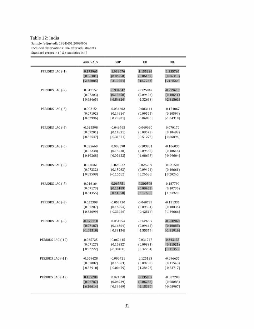
Table 12: India Sample (adjusted): 1984M01 2009M06

Included observations: 306 after adjustments

Standard errors in ( ) & t-statistics in [ ] ARRIVALS GDP ER OIL

PERIODS LAG (-1) 0.173965 1.939076 1.155226 1.355766

(0.06301) (0.06250) (0.06169) (0.06319)

[ 2.76085] [ 31.0264] [ 18.7263] [ 21.4564]

PERIODS LAG (-2) 0.047157 -0.934642 -0.125842 -0.299619

(0.07203) (0.13658) (0.09486) (0.10641)

[ 0.65465] [-6.84326] [-1.32663] [-2.81561]

PERIODS LAG (-3) 0.002154 0.034602 -0.083111 -0.174067

(0.07192) (0.14914) (0.09565) (0.10594)

[ 0.02996] [ 0.23201] [-0.86890] [-1.64310]

PERIODS LAG (-4) -0.025598 -0.046765 -0.049080 0.070170

(0.07201) (0.14931) (0.09572) (0.10489)

[-0.35547] [-0.31321] [-0.51273] [ 0.66896]

PERIODS LAG (-5) 0.035660 0.003690 -0.103981 -0.106035

(0.07238) (0.15238) (0.09566) (0.10646)

[ 0.49268] [ 0.02422] [-1.08693] [-0.99604]

PERIODS LAG (-6) 0.060461 -0.025032 0.025289 0.021584

(0.07232) (0.15963) (0.09494) (0.10661)

[ 0.83598] [-0.15682] [ 0.26636] [ 0.20245]

PERIODS LAG (-7) 0.046164 0.067751 0.300506 0.187790

(0.07173) (0.16189) (0.09462) (0.10736)

[ 0.64355] [ 0.41850] [ 3.17606] [ 1.74920]

PERIODS LAG (-8) 0.052398 -0.053730 -0.040789 -0.151335

(0.07207) (0.16254) (0.09594) (0.10836)

[ 0.72699] [-0.33056] [-0.42514] [-1.39666]

PERIODS LAG (-9) -0.075110 0.054054 -0.149797 -0.208968

(0.07187) (0.16304) (0.09642) (0.10888)

[-1.04510] [ 0.33154] [-1.55354] [-1.91916]

PERIODS LAG (-10) 0.065725 -0.062445 0.031747 0.343133

(0.07127) (0.16352) (0.09831) (0.11021)

[ 0.92222] [-0.38188] [ 0.32294] [ 3.11353]

PERIODS LAG (-11) -0.059428 -0.000721 0.125133 -0.096635

(0.07082) (0.15063) (0.09738) (0.11543)

[-0.83910] [-0.00479] [ 1.28496] [-0.83717]

PERIODS LAG (-12) 0.425280 0.024058 -0.135007 -0.007200

(0.06787) (0.06939) (0.06268) (0.08083)

[ 6.26614] [ 0.34669] [-2.15380] [-0.08907]

33

Table 13: New Zealand Sample (adjusted): 1984M01 2009M06

Included observations: 306 after adjustments

Standard errors in ( ) & t-statistics in [ ] ARRIVALS GDP ER OIL

PERIODS LAG (-1) 0.209687 1.753821 1.122243 1.397837

(0.05411) (1.08266) (0.06193) (0.06243)

[ 3.87522] [ 1.61991] [ 18.1215] [ 22.3911]

PERIODS LAG (-2) -0.001421 -1.655989 -0.225312 -0.348224

(0.05566) (1.90763) (0.09306) (0.10664)

[-0.02553] [-0.86809] [-2.42123] [-3.26552]

PERIODS LAG (-3) 0.042617 0.387992 0.072026 -0.157963

(0.05504) (1.93224) (0.09401) (0.10619)

[ 0.77430] [ 0.20080] [ 0.76619] [-1.48756]

PERIODS LAG (-4) 0.109948 -0.371421 -0.114676 0.087104

(0.05561) (2.01487) (0.09653) (0.10485)

[ 1.97709] [-0.18434] [-1.18795] [ 0.83071]

PERIODS LAG (-5) -0.076810 1.422523 -0.066743 -0.123309

(0.05632) (2.02871) (0.09980) (0.10447)

[-1.36385] [ 0.70120] [-0.66874] [-1.18035]

PERIODS LAG (-6) 0.058386 -1.295456 0.045168 -0.004895

(0.05684) (2.07204) (0.09929) (0.10394)

[ 1.02728] [-0.62521] [ 0.45489] [-0.04710]

PERIODS LAG (-7) -0.052404 -1.334034 0.179315 0.236975

(0.05707) (2.06783) (0.09861) (0.10408)

[-0.91821] [-0.64514] [ 1.81838] [ 2.27683]

PERIODS LAG (-8) 0.008957 3.905997 0.028564 -0.156073

(0.05776) (2.03115) (0.09894) (0.10514)

[ 0.15507] [ 1.92304] [ 0.28869] [-1.48440]

PERIODS LAG (-9) 0.016548 -1.675174 -0.119060 -0.194285

(0.05722) (2.01599) (0.10068) (0.10681)

[ 0.28919] [-0.83094] [-1.18257] [-1.81897]

PERIODS LAG (-10) -0.114367 0.860037 0.035878 0.310939

(0.05721) (1.91326) (0.10242) (0.10997)

[-1.99900] [ 0.44951] [ 0.35032] [ 2.82750]

PERIODS LAG (-11) -0.019700 -0.332254 -0.077161 -0.073904

(0.05779) (1.90709) (0.10131) (0.11197)

[-0.34092] [-0.17422] [-0.76165] [-0.66003]

PERIODS LAG (-12) 0.506593 -0.633159 0.046658 0.006787

(0.05560) (1.11011) (0.06572) (0.07902)

[ 9.11194] [-0.57036] [ 0.70991] [ 0.08590]

34

Table14: Netherlands Sample (adjusted): 13 318

Included observations: 306 after adjustments

Standard errors in ( ) & t-statistics in [ ] ARRIVALS GDP OIL ER

PERIODS LAG(-1) 0.206512 1.821981 1.352820 1.109015

(0.04686) (0.06277) (0.06337) (0.06244)

[ 4.40702] [ 29.0268] [ 21.3492] [ 17.7626]

PERIODS LAG (-2) -0.000297 -0.842770 -0.278532 -0.124980

(0.04807) (0.13029) (0.10695) (0.09376)

[-0.00619] [-6.46844] [-2.60444] [-1.33296]

PERIODS LAG (-3) 0.115750 -0.508655 -0.148785 0.053656

(0.04704) (0.14146) (0.10620) (0.09404)

[ 2.46074] [-3.59586] [-1.40099] [ 0.57057]

PERIODS LAG (-4) -0.111762 0.978228 0.089243 -0.133241

(0.04707) (0.14504) (0.10461) (0.09572)

[-2.37432] [ 6.74449] [ 0.85314] [-1.39206]

PERIODS LAG (-5) -0.031783 -0.486818 -0.161930 -0.131667

(0.04762) (0.15572) (0.10432) (0.09757)

[-0.66743] [-3.12614] [-1.55229] [-1.34952]

PERIODS LAG (-6) -0.108061 -0.174290 -0.014140 0.018526

(0.04775) (0.15652) (0.10474) (0.09720)

[-2.26313] [-1.11355] [-0.13500] [ 0.19059]

PERIODS LAG (-7) 0.106543 0.427477 0.218982 0.266126

(0.04791) (0.15584) (0.10612) (0.09684)

[ 2.22390] [ 2.74298] [ 2.06362] [ 2.74805]

PERIODS LAG (-8) -0.070166 -0.277760 -0.120472 0.007305

(0.04838) (0.15737) (0.10688) (0.09815)

[-1.45037] [-1.76502] [-1.12712] [ 0.07443]

PERIODS LAG (-9) 0.169098 -0.012965 -0.221385 -0.122531

(0.04840) (0.15137) (0.10643) (0.10021)

[ 3.49381] [-0.08566] [-2.08012] [-1.22278]

PERIODS LAG (-10) -0.171316 0.153572 0.324356 -0.020749

(0.04912) (0.14779) (0.10850) (0.10210)

[-3.48750] [ 1.03915] [ 2.98944] [-0.20322]

PERIODS LAG (-11) 0.095549 -0.129327 -0.087487 0.045050

(0.04988) (0.13904) (0.11221) (0.10155)

[ 1.91571] [-0.93015] [-0.77968] [ 0.44362]

PERIODS LAG (-12) 0.674469 0.051816 0.034384 -0.040293

(0.04837) (0.06680) (0.08051) (0.06629)

[ 13.9435] [ 0.77572] [ 0.42707] [-0.60779]

Table 15: USA

35

Sample (adjusted): 1984M01 2009M06

Included observations: 306 after adjustments

Standard errors in ( ) & t-statistics in [ ] ARRIVALS GDP ER OIL

PERIODS LAG(-1) 0.241659 1.898732 1.206175 1.333614

(0.05344) (0.06218) (0.06144) (0.06367)

[ 4.52214] [ 30.5377] [ 19.6325] [ 20.9446]

PERIODS LAG (-2) 0.042369 -0.870345 -0.236230 -0.257229

(0.05610) (0.13256) (0.09668) (0.10562)

[ 0.75523] [-6.56559] [-2.44338] [-2.43535]

PERIODS LAG (-3) -0.020489 -0.537307 -0.001579 -0.192322

(0.05648) (0.14103) (0.09816) (0.10454)

[-0.36278] [-3.80976] [-0.01609] [-1.83968]

PERIODS LAG (-4) -0.023528 0.958789 -0.046190 0.107956

(0.05667) (0.14481) (0.09781) (0.10291)

[-0.41516] [ 6.62090] [-0.47224] [ 1.04900]

PERIODS LAG (-5) -0.037217 -0.446619 -0.097136 -0.131965

(0.05700) (0.15628) (0.09770) (0.10287)

[-0.65294] [-2.85788] [-0.99421] [-1.28282]

PERIODS LAG (-6) -0.027513 -0.131686 0.068894 0.018714

(0.05723) (0.15742) (0.09769) (0.10258)

[-0.48076] [-0.83652] [ 0.70521] [ 0.18243]

PERIODS LAG (-7) 0.036976 0.249021 0.115393 0.202517

(0.05778) (0.15782) (0.09750) (0.10327)

[ 0.63998] [ 1.57788] [ 1.18352] [ 1.96103]

PERIODS LAG (-8) -0.010420 -0.117533 0.137553 -0.157588

(0.05768) (0.15640) (0.09724) (0.10491)

[-0.18066] [-0.75151] [ 1.41458] [-1.50217]

PERIODS LAG (-9) 0.012066 -0.220534 -0.233157 -0.220448

(0.05754) (0.14415) (0.09892) (0.10637)

[ 0.20968] [-1.52986] [-2.35695] [-2.07241]

PERIODS LAG (-10) -0.026239 0.413320 0.004695 0.341567

(0.05764) (0.14093) (0.10178) (0.10908)

[-0.45521] [ 2.93282] [ 0.04613] [ 3.13148]

PERIODS LAG (-11) 0.108874 -0.199817 0.117068 -0.096378

(0.05728) (0.13277) (0.10151) (0.11267)

[ 1.90089] [-1.50499] [ 1.15322] [-0.85539]

PERIODS LAG (-12) 0.561213 0.003680 -0.096251 0.038092

(0.05684) (0.06294) (0.06383) (0.07852)

[ 9.87275] [ 0.05847] [-1.50786] [ 0.48512]

36

Table 16: UK Sample (adjusted): 1984M01 2009M06

Included observations: 306 after adjustments

Standard errors in ( ) & t-statistics in [ ] ARRIVALS GDP ER OIL

PERIODS LAG(-1) 0.297596 1.897097 1.209057 0.575948

(0.05234) (0.06275) (0.06208) (0.50378)

[ 5.68583] [ 30.2347] [ 19.4758] [ 1.14325]

PERIODS LAG (-2) 0.078598 -0.876194 -0.309500 -0.612502

(0.05581) (0.13406) (0.09655) (0.78349)

[ 1.40829] [-6.53571] [-3.20564] [-0.78176]

PERIODS LAG (-3) -0.055542 -0.617065 0.137603 0.432554

(0.05540) (0.14238) (0.09793) (0.79474)

[-1.00254] [-4.33383] [ 1.40506] [ 0.54427]

PERIODS LAG (-4) 0.065020 1.116139 -0.084618 -0.559589

(0.05595) (0.14641) (0.09874) (0.80126)

[ 1.16213] [ 7.62313] [-0.85699] [-0.69838]

PERIODS LAG (-5) -0.165098 -0.478993 -0.184846 0.357910

(0.05602) (0.16218) (0.09916) (0.80470)

[-2.94738] [-2.95351] [-1.86408] [ 0.44477]

PERIODS LAG (-6) -0.082338 -0.229412 0.132380 -0.890803

(0.05614) (0.16259) (0.09906) (0.80386)

[-1.46675] [-1.41100] [ 1.33639] [-1.10816]

PERIODS LAG (-7) 0.133111 0.331932 0.146529 0.630027

(0.05672) (0.16233) (0.09781) (0.79373)

[ 2.34702] [ 2.04485] [ 1.49810] [ 0.79375]

PERIODS LAG (-8) 0.032006 -0.127303 0.072269 -1.303268

(0.05698) (0.16341) (0.09806) (0.79573)

[ 0.56170] [-0.77906] [ 0.73702] [-1.63783]

PERIODS LAG (-9) -0.064614 -0.142622 -0.166253 2.132714

(0.05713) (0.14908) (0.10239) (0.83089)

[-1.13096] [-0.95666] [-1.62374] [ 2.56679]

PERIODS LAG (-10) 0.051605 0.205529 -0.119598 -0.909797

(0.05721) (0.14230) (0.10448) (0.84788)

[ 0.90199] [ 1.44430] [-1.14467] [-1.07302]

PERIODS LAG (-11) 0.043563 -0.056854 0.170406 0.025057

(0.05676) (0.13408) (0.10265) (0.83299)

[ 0.76748] [-0.42404] [ 1.66011] [ 0.03008]

PERIODS LAG (-12) 0.558117 -0.023531 -0.069891 0.137288

(0.05415) (0.06489) (0.06431) (0.52184)

[ 10.3060] [-0.36263] [-1.08687] [ 0.26308]

Model Specification

37

Table 17: Model representation for the lagged variables of vector x

Arrivals GDP RER Oil prices

Australia 1, 12 1,8,11 1,7 1,2,10

France 1, 12 1,4 1,7 10

Germany 1, 12 1,2 1,2,7 1,2,10

India 1, 12 1,2 1,7 1,10

Netherlands 1, 12 1,2 1,7 1,2

New Zealand 1, 12 1,8 1,2 1,10

UK 1, 12 1,2,4 1,2,5 1,8

USA 1, 12 1,2,4 1,2 1,2,10

Data manipulations for foreign arrivals:

There is omitting data for a number of months for foreign tourist arrivals, but it impossible to leave

them blank as it will have large affects on yearly totals and will be misrepresentative. Therefore an

amount was calculated using the following equations and inputted for each of the month missing

variables. The subscript t represents the current period were there is missing data, the t-1 subscript

refers to the month of the previous period (corresponding to the month in the previous year) while

t+1 subscript refers to the month of the next period (corresponding to the month in the next year)

This was done for the following data points:

MAY 1985 - India

FEB 1989 -all countries

NOV 1994 -Brazil, China, India and Spain

DEC 1994 -Brazil

JAN 1996- JULY 1996 - Brazil, China, India and Spain

AUG 1996 -Brazil

SEPT 1996 - Brazil, China, India and Spain

OCT 1996 - Brazil, China, India and Spain

DEC 1996 - Brazil, China, India and Spain

For the following points no data was published for foreign arrivals from Spain, therefore the

38

Portuguese arrivals which is of a similar nature was used as a proxy:

JAN 2009

FEB 2009