south african real interest rates in comparative ... and publications/attachments... · south...

South African real interest rates in comparative perspective: theory and evidence

by B Kahn and G N Farrell

Occasional Paper No 17

February 2002

South African Reserve Bank

Contents

Page

1. Introduction ............................................................................ 1

2. Theoretical considerations ...................................................... 2

3. Determinants of real interest rates .......................................... 33.1 Changes in savings........................................................ 33.2 Changes in investment .................................................. 43.3 Monetary policy ............................................................ 43.4 Financial market deregulation ........................................ 43.5 Risk premiums .............................................................. 53.6 The impact of taxation .................................................. 5

4. Measurement issues................................................................ 54.1 Time horizon .................................................................. 54.2 Which rate (given the time horizon)? .............................. 64.3 Measures of inflationary expectations ............................ 64.4 Does the choice of an inflation expectations proxy

really matter? ................................................................ 8

5. Historical trends ...................................................................... 9

6. Linkages between real interest rates........................................ 166.1 Testing real interest rate linkages.................................... 176.2 I(1)/I(0) unit root tests on the real interest differential ...... 186.3 A fractional integration approach to real interest

rate differentials.............................................................. 19

7. Implications and conclusions .................................................. 21

Appendix 1: The data ...................................................................... 22

Appendix 2: Unit root tests .............................................................. 23

References ...................................................................................... 25

SA RESERVE BANK

OCCASIONAL PAPER No 17

Ronel

List of tables

1. Real interest rates since 1950 ................................................ 132. Short-term real interest rate differentials .................................. 143. Long-term real interest rate differentials .................................. 154. DF-GLS� and KPSS tests on short-term real interest

rate differentials ...................................................................... 185. GPH estimates of the fractional differencing parameter d ........ 20

List of figures

1. Figure 1: South Africa: alternative measures of short-termreal interest rates .................................................... 9

2. Figure 2: Short-term real interest rates .................................. 103. Figure 3: Long-term real interest rates.................................... 124. Figure 4: Country risk measured by bond spreads ................ 15


SA RESERVE BANK

South African real interest rates in comparative perspective: theory and evidence

by B Kahn and G N Farrell1

Real interest rates lie at the heart of the transmission mechanism of monetary policy. Although in thelong run real interest rates are determined by real factors such as the propensity to save and the pro-ductivity of capital, monetary policy can impact on the real interest rate in the short to medium term.This paper surveys the theoretical and applied literature on real interest rates from a South African per-spective, and compares South African real interest rates in an international and historical context. Thenature of the linkages between South African and international real interest rates is also consideredusing a fractional integration approach. What emerges from the analysis is that, viewed historically,South Africa’s real interest rates tended to broadly follow international trends. Although short-term realrates in South Africa have recently been high by historical standards and relative to some low-inflationcountries, it is argued that this situation cannot be seen in isolation from the current monetary policyframework and the level of the inflation rate relative to the target. Current rates reflect to a certain extentthe Reserve Bank’s overriding commitment to the inflation target.

1. Introduction

Real interest rates lie at the heart of the transmission mechanism of monetary poli-cy. Investment spending is affected by the cost of capital, and this provides a linkbetween the financial sector and the macroeconomy. The business cycle and thetransmission of economic policies in turn are influenced by business investment aswell as household investment and consumption.

Although in the long run real interest rates are determined by real factors such as thepropensity to save and the productivity of capital, monetary policy can impact on thereal interest rate in the short to medium term. In South Africa attention was focusedon real interest rates particularly in the aftermath of the 1997/98 Asian crisis, whenshort-term real interest rates became highly positive. This paper attempts to put theissue of South African real interest rates into historical and comparative perspective.The main focus is on comparing South Africa’s real interest rates to those prevailinginternationally, and on drawing some policy conclusions.

What emerges from the analysis is that, viewed historically, South Africa’s real inter-est rates tended to broadly follow international trends. The periods when there weresignificant exceptions were during the 1980s, around the debt crisis and financialsanctions period, and since 1995. This is particularly the case with the short-termrate. Although South Africa’s long-term rates do not seem out of line with interna-tional levels, particularly once we account for risk premiums, short-term rates arehigher, due in part to monetary policy decisions. This situation is however consistentwith the experiences of other countries (e.g. Australia and New Zealand) that haveopened up their capital accounts, and at the same time also adopted strong anti-inflation policies. Where the actual inflation rate is above the target rate, we wouldexpect short-term real rates to be high.

This paper is organised as follows: Section 2 briefly considers some of the theoret-ical issues relating to real interest rates, and Section 3 discusses the determinantsof real interest rates. Section 4 considers measurement issues: many of the differ-ences in observed rates are affected by how we actually measure real interest rates,particularly inflation expectations. Section 5 analyses historical trends in real interestrates in South Africa and internationally, and looks at the various causes of higherinterest rates internationally since the 1980s. The question of whether current South

1

SA RESERVE BANK


1 The views expressed inthis paper are those of theauthors and do not necessarilyrepresent those of the SouthAfrican Reserve Bank orReserve Bank policy. Whileevery precaution is taken toensure the accuracy of information, the South AfricanReserve Bank shall not be liableto any person for inaccurateinformation or opinions con-tained herein.

African interest rates are high, in an historical and international context, is addressedin this section. Section 6 presents empirical evidence of a long-run linkage betweenSouth African and international real interest rates, and Section 7 concludes.

2. Theoretical considerations

The standard form of expressing the real interest rate is based on the Fisher equation, in terms of which the real interest rate (r e

t) on an m-period bond held tomaturity in period t+m is equal to the corresponding nominal interest rate minus theexpected inflation rate over the period:2

r et ≅ it – Etπt (1)

where it is the nominal interest rate on the m-period bond held to maturity in periodt+m, and Etπt is the expectation at time t of the rate of inflation from period t to t+m.

In the open economy context, if capital is perfectly mobile and real exchange ratesconverge to their equilibrium levels, ex ante real interest rates should move togeth-er in the long run. To see this, consider the analytical underpinnings of the relation-ship between international real interest rate differentials and real exchange rates. Thedifferential between nominal interest rates at home and abroad may be described bythe uncovered interest parity relationship with a risk premium

it – i*t = [Etst+m – st ] + �t (2)

where st is the (log of the) nominal exchange rate (expressed as home currency toforeign, e.g. rand per dollar), Etst+m is the expectation at time t of this exchange ratein period t+m, and �t is a risk premium. A star superscript denotes a foreign variable.

By definition, the real exchange rate qt is given by

qt = st – pt + p*t (3)

where pt ( p*t) is the log of the home (foreign) price level. Using the approximations

Et pt+m ≅ pt + Etπt ; Et p*t+m ≅ p*t + Etπ*t (4)

where Etπt (Etπ*t) is the expectation at time t of inflation over the period from t to t+mat home (abroad), and substituting from the expectation of (3) into (2)

it – i*t = [Etqt+m + (pt + Etπ t ) – (p*t + Etπ*t ) ] – [qt + pt – p*t ] + �t (5)i.e.

(it – Etπ t ) – (i*t – Etπ*t) = [Etqt+m – qt] + �t (6)

and using the Fisher equation to define the real interest rates rt, r*t

rt = it – Etπ t ; r*t = i*t – Etπ*t (7)

the real uncovered interest parity relationship with a risk premium is

rt – r*t = [Etqt+m – qt] + �t

orrt = r*t + [Etqt+m – qt] + �t (8)

2 OCCASIONAL PAPER No 17

SA RESERVE BANK

2 More precisely, the equation is given by

(1+ r et) = (1+ it)/(1+ Etπt)

or r e

t = (it - Etπt)/(1+ Etπt).

The extent to which real interest rates move together in practice may therefore shedsome light on either the degree of capital mobility, real exchange rate convergence,or the presence of a time-varying risk premium. It follows therefore that to the extentthat real interest parity fails to hold, a risk premium or discount can be said to exist,reflecting exchange rate or political uncertainties, administrative restrictions or otherconsiderations. Increased liberalisation of capital markets in the 1980s should havestrengthened the link between different interest rates.

3. Determinants of real interest rates

The classical view of the real interest rate is that it reflects the forces of productivityand thrift – the (marginal) productivity of capital, which determines the demand forcapital, and the forces behind saving behaviour. A more Keynesian view is that “the”interest rate is determined in stock markets as portfolio holders choose betweensafe and risky assets and make intertemporal choices. The traditional view arguesthat there is no impact of monetary policy in the long run, and in the long run the realinterest rate is only determined by the fundamentals of productivity and thrift.

However a new view argues that intertemporal arbitrage should ensure that short-term interest rates, long-term interest rates, and expectations (including expecta-tions about what policy makers will do) are closely linked. Allsopp and Glyn (1999)for example argue that given that there are different policy regimes, there can be nopresumption that there is a unique fundamental, equilibrium, real long-term interestrate which will tend to rule independently of the monetary policy regime and thestance of other policies. Their framework leads them to conclude that “it would bewrong to think of the real interest rate as determined just by the fundamentals of pro-ductivity and thrift and independent of monetary policy. On the contrary, one wouldexpect interest rates to depend, for long periods, on the monetary policy regime andthe stance of other policies, such as fiscal policy” (Allsopp and Glyn, 1999: 15). Thisimplies that the real interest rate is not necessarily constant over time, i.e. the equi-librium real interest rate can change as the policy regime changes.

Much of the empirical literature on real interest rates has focused on the causes ofthe higher levels of interest rates since the 1980s. This section gives an outline ofsome of the factors that have determined the real interest rate levels or movements.

3.1 Changes in savings

The role of reduced current and prospective saving in driving up interest rates, e.g.increased public dissaving through increased budget deficits, is seen by Blanchardand Summers (1984) as a possible cause of higher real interest rates in the US inthe 1980s, although their findings do not give strong evidence for this. SimilarlyMishkin (1988) and Huizinga and Mishkin (1986) underplay the impact of higher bud-get deficits.

Orr et al. (1995) show that much of the fall in saving in the 1980s was due to thereduction in government saving. The decline in savings ratios is linked to financial lib-eralisation (which may have reduced saving propensities by removing liquidity con-straints); lower inflation (reduced precautionary saving) and longer-term demographicfactors (an ageing population implies lower saving). In a similar vein Atkinson andChouraqui (1985) identify the Federal budget deficit in the US, and a shift in the fis-cal/monetary policy mix in Europe where higher budget deficits had to be financed inthe face of increasingly non-accommodative monetary policy.

3

SA RESERVE BANK


Helbling and Wescott (1995), Howe and Piggott (1991), Ford and Laxton (1999),and Chadha and Dimsdale (1999) show that higher levels of government debt areassociated with higher real interest rates. The growth of public debt relative to GDPwill require agents to adjust their portfolios to hold more government securities. Thereal yield on government bonds must rise to bring about this change in portfolios.

3

3.2 Changes in investment

Blanchard and Summers (1984) identify the increased attractiveness of investmentowing to increased profitability or reduced uncertainty, as a major cause of higherinterest rates in the 1980s. Similarly Orr et al. (1995) argue that higher returns tocapital, which were a consequence of structural economic reforms, trade liberalisa-tion, lower inflation, and the elimination of restrictions on direct foreign investmentcaused investment ratios to rise in the 1980s. Furthermore, growing demands forinvestment funds in non-OECD countries also represented a source of upward pres-sure on interest rates. Atkinson and Chouraqui (1985) argue, however, that althoughincreased investment is important, it is difficult to determine empirically.

3.3 Monetary policy

As noted above, the traditional view has been that monetary policy has no impacton the real interest rate in the long run, as argued in Chadha and Dimsdale (1999).This assumes that the full adjustment of nominal interest rates to inflation takesplace. In reality, the process is likely to be slow, hence changes in the rate of mone-tary growth may be expected to have persistent effects on real interest rates andhence on other real variables, such as output and employment. Blanchard andSummers (1984) emphasise the anticipation of sustained tight monetary policy, i.e.tight monetary policy that is expected to maintain interest rates at values higher thantheir equilibrium level in the short run.

High real interest rates have been observed in various countries for several monthsafter the adoption of disinflation programmes. According to Kaminsky andLeiderman (1996), six months after the start of stabilisation plans in Argentina, Israeland Mexico in the mid-1980s, real interest rates were still of the order of 40-50 percent per year. Interest rates of about 100 per cent were observed six months afterthe Bolivian stabilisation in 1985. High real interest rates of 5-6 per cent wereobserved in OECD countries following reductions in the inflation rates in the early1980s. One explanation is a reflection of a shortage of liquidity induced by contrac-tionary monetary policy. Kaminsky and Leiderman offer an alternative explanationwhich is that high ex post real rates can be explained in terms of an ex post error ininflation expectations, which reflects a lack of credibility of the low-inflation policy. Ifthere is an expectation that high inflation will return, nominal rates will remain high.Over time as the new policy gains credibility, expectations of inflation will be reviseddownward, and nominal (and real) interest rates exhibit a gradual decline. Becauseexpected inflation exceeds the actual outcome, ex ante real interest rates will belower than those observed ex post.

3.4 Financial market deregulation

The regulation and deregulation of capital markets will have consequences for realinterest rates. Governments faced with the financing of large budget deficits haveattempted to reduce their own costs of borrowing by imposing restrictions on otherborrowers. The removal of such restrictions will tend to raise real interest rates, for


SA RESERVE BANK

3 This is qualified by the neo-Ricardian view that increases inthe public debt will have noeffect on the level of real interestrates as increased public bor-rowing is balanced by increasedsaving by the private sector toanticipate future tax liabilities.

example the removal of prescribed asset requirements in South Africa during the1980s and the relaxation of exchange controls. Similarly, Jenkinson (1999) hasargued that real interest rates in the UK increased following the abolition of pre-scribed asset requirements as well as the abolition of exchange control in 1979.

3.5 Risk premiums

High rates on long bonds do not necessarily imply high expected short rates, butmay instead reflect an increase in the risk premium required to hold long bonds, asreflected in Equation 8 above. Here changes in asset prices and returns reflect port-folio shifts rather than shifts in saving or investment. Over time the risk premiums ondifferent types of security could be expected to vary, and this could help to explainchanges in the real interest rate on individual types of security.

3.6 The impact of taxation

Atkinson and Chouraqui (1985) emphasise the impact of taxation although they findthat it is difficult to confirm the influence. Similarly Chadha and Dimsdale (1999)argue that lower business taxes and high profitability would have contributed to thehigh real rates of the 1980s.

Although, as seen, there are a number of factors influencing the real interest rate,Atkinson and Chouraqui argue that all of these could have had some influence atone time or another, but none has a dominant monocausal role.

4. Measurement issues

One of the most intractable problems encountered in the study of real interest ratesis the problem of measurement. This includes not only the issue of measuring infla-tion expectations, but also of deciding which interest rate to measure and the timehorizon over which it should be measured. Blinder, commenting on Blanchard andSummers (1984), notes that the margin of uncertainty when measuring real interestrates is enormous. He shows, using Blanchard and Summers’ data, that “from 1978to 1984 … the real short term rate in the United Kingdom went up by either 8.2points or 2.3 points depending on how you measure it. Between 1980 and 1983 …the real short rate in West Germany either rose 1.9 points or fell 1.8 points!”(Blanchard and Summers, 1984: 326). He argues that the margin of error withrespect to long rates is even larger, and concludes that inferring the slope of the termstructure of real interest rates is a hazardous and probably impossible enterprise inthe absence of indexed bonds.

4.1 Time horizon

In general, the focus of empirical studies has been on long-term rates on thegrounds that they impact more fundamentally on savings and investment decisionsthan short-term rates. Jenkinson (1999) argues for example that a 5-10 year timehorizon is most relevant to most companies’ investment decisions, while Scott(1993) also emphasises the fact that the long-term rate is a better indicator of thefuture cost of servicing the national debt.

However, since monetary policy has a direct effect on short-term rates, and if we areinterested in the impact of official actions on interest rates, then it is necessary to lookat short-term rates. It is also often the case that smaller businesses, particularly in

5

SA RESERVE BANK


South Africa, finance themselves not through equity finance or long-term borrowingbut through short-term overdraft facilities. In addition, most consumer durable expen-diture as well as mortgage finance is related to the short-term prime overdraft rate.

Furthermore, the problems of calculating ex ante real interest rates (discussedbelow) are reduced when dealing with short-term rates because systematic errorsin inflation forecasting are less likely over short time horizons. This makes actualinflation a good proxy for expected inflation and so expected and realised realrates will be similar. Blanchard and Summers (1984) place more emphasis on thecomputation of real ex post short rates on the grounds that the computation oflong-term rates (because of the problem of measuring long-term inflationaryexpectations) is necessarily arbitrary.

4.2 Which rate (given the time horizon)?

In analysing trends in real interest rates, inevitably a single rate is examined. Howeveras Orr et al. (1995) note, this ignores the fact that different agents are charged dif-ferent rates, that there are cross-country differences in the relative importance ofmaturity structures in financing, and that different risk premiums face similar cate-gories of borrowers. In addition, different tax regimes affect the real interest rate,which further complicates cross-country comparisons. A further factor complicatingcross-country comparisons is the fact that financial liberalisation occurred at differ-ent times and speeds across countries, affecting the measurement of effective interest rates and possibly putting upward pressure on real rates through a negativeimpact on saving.

Various nominal interest rates are used in the literature as a basis for real interest rate cal-culations. For example, Jenkinson (1999) and Breedon et al. (1999) focus on returns ongovernment securities to approximate the return on a riskless asset. Chadha andDimsdale (1999) and Ford and Laxton (1999) use a money-market rate for the short-termreal interest rate on the grounds that it is closer to the borrowing costs of the private sector but will involve risk premiums compared to government securities.

4.3 Measures of inflation expectations

Given that real rates are the nominal yields on bonds adjusted for expected inflation overthe life of the bond, the problem arises in measuring the unobservable long-run infla-tionary expectations. This section briefly reviews some of the different methodologiesused to estimate expected inflation. In general, five different approaches may be identified.

(i) The simplest approach to estimating expected inflation is to use a measure ofobserved past inflation. Assuming again an m-period bond, this approachresults in what is called the conventional real interest rate (r c

t )

r ct = it – πt-j,t (9)

where πt-j,t is the rate of inflation from period t-j to t. Real interest rates mea-sured in this way are simple to calculate, but are clearly problematic wheninflation expectations are not static. This is especially the case when long-termexpectations are involved.


SA RESERVE BANK

(ii) The second approach uses the realised inflation rate over the period as a proxyfor expected inflation. This generates the ex post measure of the real interestrate (rp

t)

rpt = it - π*t,m (10)

where π*t,m is the actual rate of inflation from period t to t+m. The ex post realinterest rate is not known when decisions are taken, so its usefulness dependson the extent to which expectations approximate realised outcomes.4

(iii) An alternative approach is to compute an inflation forecast from a time seriesmodel such as an ARIMA model, or by “smoothing” the inflation series using, forexample, a long moving average or some smoothing technique such as aHodrick-Prescott filter. In the former case, current price increases are treatedsolely as a function of constant and past values of inflation and this method istherefore subject to the criticism that the procedure is too inflexible and fails tomake use of some information which is both relevant and available.5 Smith (1996)uses a quarterly ARMA forecast of CPI inflation and similarly, Begum (1998) usesthe forecast from an ARIMA (4,1) model of inflation. Blanchard and Summers(1984) and Barro and Sala-i-Martin (1990) make expected inflation a mathemat-ical function of past inflation.

Computing expected inflation by “smoothing” the inflation series is a commonlyused technique. For example, Pain and Thomas (1997) proxy inflation expecta-tions over the next three months by taking a simple four-quarter moving ave-rage of quarterly inflation. Smith (1996) and Pain and Thomas (1997), inanalysing long-term rates, use a two-year centred moving average of CPI infla-tion. Orr et al. (1995) proxy trend inflation by the low-frequency component ofthe GDP deflator computed by a Hodrick-Prescott filter. This measure incorpo-rates both forward and backward-looking elements of the inflation process in atype of “two-way averaging” process, and therefore uses information not avail-able to ex ante forecasts.

A problem when working with long-term rates is that if we are for examplelooking at 10-year rates, ten years of observations are lost if we are measur-ing expectations on an ex ante basis. Most studies therefore use forecastswhich are confined to one or two years ahead at most. Scott’s (1993) view isthat the best procedure would be to do a thorough historical study of eachperiod for which an estimate of long-term inflationary expectations is required.This has major difficulties in terms of constructing a consistent time series. Theproblem is compounded if cross-country comparisons are made. Withrespect to long-term rates, Chadha and Dimsdale (1999) contend that thedetermination of real long-term ex ante rates poses problems because of lackof knowledge about expected future rates of inflation and that holding periodrates of return may well also differ from yields to maturity.

(iv) The fourth approach used in the literature is to use survey data on inflationaryexpectations. Mishkin (1988), however, argues that survey-based measureshave their own problems as survey respondents may have little incentive torespond accurately. Furthermore he argues that “the behaviour of marketexpectations is driven by economic agents at the margin who are eliminatingunexploited profit opportunities. Market expectations, therefore, are unlikely tobe well measured by the average expectations of survey respondents”(Mishkin, 1988: 1064).

7

SA RESERVE BANK


4 In this regard, if rationalexpectations are assumed, theinflation forecast error

εt,m = Etπt - π*t,m

is a martingale difference.Furthermore, from the definitionsprovided above,

rpt+ π*t,m = ret + Etπti.e.rpt = ret + (Etπt - π*t,m)

= ret + εt,m

Under rational expectations,then, the ex post and ex ante realinterest rates differ by a stationarycomponent εt,m . The two rateswill therefore have the same long-run time series properties in that atest for a unit root in the ex postreal interest rate series may beinterpreted as a test for a unit rootin the ex ante real interest rate.Also, it follows that the ex postrate will tend to exhibit less per-sistence than the ex ante rate(see Section 4).

5 See for example Scott(1993: 5).

An additional problem for time-series analysis is that there are very few seriesof inflationary expectations based on survey data.

(v) Finally, the emergence of index-linked government bonds has provided adirect measure of long-term real rates and allows for direct measures of infla-tionary expectations. In the UK, for example, the direct measure for long-termreal rates provided by index-linked bonds is less variable than most proxymeasures. Also, the index-linked yield tends to be below the proxy when cur-rent inflation is relatively low by historical standards and above the proxy wheninflation is relatively high, which suggests that long-term inflationary expecta-tions are relatively slow to respond to current actual inflation.

6

The difference between the yield on non-indexed and index-linked govern-ment bonds provides one measure of long-term inflation expectations,although it may also capture the effects of factors other than inflation expec-tations, including differences in tax treatment, inflation uncertainty and liquidi-ty premiums (Orr et al., 1999). In addition there are important indexation lagsin inflation-proof bonds and so they cannot be considered to be pure realbonds. Finally, the absence of a long historical data run of real yields makesinferences on long-term patterns highly problematic, especially in the case ofSouth Africa where index-linked bonds are a relatively new phenomenon.7

4.4 Does the choice of an inflation expectations proxy really matter?

Despite the differences in approaches to measuring expectations, Blanchard andSummers (1984) found little difference over the long run between ex post and exante measures of the real rates. They attribute this to the argument that over the verylong run the subjective prior about the inflation process is more likely to coincide withits ex post realisation.

A comparison by Orr et al. (1995) of a range of proxies for inflationary expectationsconcludes that medium-term trends in real interest rates are not substantially affect-ed by the exact choice among a range of reasonable proxies for trend inflation,although the timing of turning points can differ significantly in periods where inflationis highly variable. Chadha and Dimsdale (1999) argue that as long as agents do notmake systematic errors in their forecasts of inflation, the difference between predic-tions of inflation and actual inflation is likely to be small, particularly over long periodsof time.

However, as noted above, Blinder did find considerable differences (Blanchard andSummers, 1984). Similarly, Atkinson and Chouraqui (1985) show that differencesbetween real long-term interest rates as conventionally measured and their ex postvalues have often been substantial. They argue that in many cases a failure to antici-pate the inflation of the 1973-75 period resulted in significantly negative real returnsdespite real rates that were apparently positive. They found that although at timesthere were differences between the conventional and the ex ante measures, oftenthey were similar. Also, the substantially negative conventional real interest ratesexisting around 1974-75 were not, except in Italy, realised ex post. It would appearthat the differences between the measures become more pronounced during periods of inflation volatility and unexpected exchange rate changes.


SA RESERVE BANK

6 This implies that countrieswith a history of high inflation willtend to pay significant inflationpremiums in nominal bond yieldsuntil market participants are con-vinced of sustained price stability.

7 In the South African case,the first issue was set at 6,5 percent, which was the rate (arbi-trarily) set by the Treasury, ratherthan being a true measure ofmarket expectations.

Figure 1 shows various alternative measures for South Africa, and it can be seenthat although these measures do generally move together, the ex post measuretends to deviate from the other measures during periods when the inflation trend ischanging. So, for example, the lower ex post real interest rates of the early to mid-1970s reflected a situation where inflation was higher than expected, whereas theearly 1990s was a period when the inflation rate fell by more than expected. Thevarious ex ante measures move sufficiently closely to ignore the differences. Since1993 the different measures, including the ex post measures, have coincided suf-ficiently to ignore this potential problem.

5. Historical trends

Given the multiplicity of alternative measures, differences in measured real interestrates are inevitable. Despite these problems and differences, however, certain com-mon trends emerge from the literature. Most of the existing analyses of historicaltrends in real interest rates have been conducted on industrialised countries, andexamine three main subperiods of the post-1950 experience: the 1950-69 periodcorresponding with the “golden age” of the post-World War II boom; the 1970-79period corresponding with the turbulence and inflation of the oil crises; and the post-1980 period which was characterised by greater financial market liberalisation andmore emphasis on inflation control.8 A common result in these studies is that the firstof these periods was characterised by positive real interest rates averaging around 2per cent, the second by negative or extremely low positive real rates, and the 1980sand 1990s by positive real rates which were higher than in the previous periods,although generally real rates in the 1990s tended to be lower than in the 1980s.

9

SA RESERVE BANK


Figure 1 South Africa: alternative measures of short-term real interest rates

Per cent

1950 1955 1960 1965 1970 1975 1980 1985 1990 1995 2000

Conventional short-term real interest rateEx post short-term real interest rateEx ante short-term real interest rate (Hodrick-Prescott)Ex ante short-term real interest rate (3-year backward weighted average)

-15

-10

-5

0

5

10

15

20

8 See for example Allsoppand Glyn (1999) and the studies cited therein, andLevy and Panetta (1996).

In this study, short and long-term real interest rates were calculated for South Africaand a selection of other countries, at the annual and monthly frequencies. A dis-cussion of the data used to calculate these real interest rates appears in Appendix1, and plots of the rates are presented in Figures 2 – 3. The discussion in this sec-tion is based on the annual data set, since this covers the longest time-span.However the trends that emerge at the various frequencies are largely consistent. Inline with the studies of the evolution of real interest rates cited above, the plots sug-gest that the South African experience in the post-1950 period may usefully beexamined over the same three periods.


SA RESERVE BANK

-15

-10

-5

0

5

10

15

1950 1960 1970 1980 1990 2000

South Africa USA

Per cent

South Africa and USA

-15

-10

-5

0

5

10

15

1950 1960 1970 1980 1990 2000

South Africa Canada

Per cent

South Africa and Canada

-20

-15

-10

-5

0

5

10

15

1950 1960 1970 1980 1990 2000

South Africa Japan

Per cent

South Africa and Japan

-15

-10

-5

0

5

10

15

1950 1960 1970 1980 1990 2000

South Africa Germany

Per cent

South Africa and Germany

Figure 2 Short-term real interest rates

11

SA RESERVE BANK

-20

-15

-10

-5

0

5

10

15

1950 1960 1970 1980 1990 2000

South Africa France

Per cent

South Africa and France

-20

-15

-10

-5

0

5

10

15

1950 1960 1970 1980 1990 2000

South Africa United Kingdom

Per cent

South Africa and United Kingdom

-15

-10

-5

0

5

10

15

1950 1960 1970 1980 1990 2000

South Africa Australia

Per cent

South Africa and Australia

-15

-10

-5

0

5

10

15

1950 1960 1970 1980 1990 2000

South Africa New Zealand

Per cent

South Africa and New Zealand

Figure 2 Short-term real interest rates (continued)

South Africa and Chile

-20

-10

0

10

20

30

40

50

1950 1960 1970 1980 1990 2000

South Africa Chile

Per cent

-50

-40

-30

-20

-10

0

10

20

30

1950 1960 1970 1980 1990 2000

South Africa Mexico

Per cent

South Africa and Mexico



SA RESERVE BANK

Figure 3 Long-term real interest rates

South Africa and USA

-6

-4

-2

0

2

4

6

8

10

12

1950 1960 1970 1980 1990 2000

South Africa USA

Per cent

South Africa and Canada

-10

-5

0

5

10

15

1950 1960 1970 1980 1990 2000

South Africa Canada

Per cent

South Africa and Japan

-20

-15

-10

-5

0

5

10

15

1950 1960 1970 1980 1990 2000

South Africa Japan

Per cent

South Africa and Germany

-6

-4

-2

0

2

4

6

8

10

12

1950 1960 1970 1980 1990 2000

South Africa Germany

Per cent

South Africa and France

-15

-10

-5

0

5

10

15

1950 1960 1970 1980 1990 2000

South Africa France

Per cent

South Africa and United Kingdom

-15

-10

-5

0

5

10

15

1950 1960 1970 1980 1990 2000

South Africa United Kingdom

Per cent

In the 1950-69 period, as Table 1 shows, South African real interest rates were relativelylow, but positive, with the short-term ex post real interest rate averaging 1,2 per centand the long-term rate 1,9 per cent. From a comparative international perspective,South Africa’s average short-term real interest rate over this period was above that ofFrance (-0,6 per cent), but lower than or equal to those of the other countries surveyed.For example the US rate was 1,2 per cent, Germany 2,0 per cent, and New Zealand1,5 per cent. The average long-term rate of 1,9 was in line with that of the UK, US andJapan, but well below that of Germany (4,4 per cent). Australian and New Zealand rateswere extremely low. As mentioned earlier, financial market and other restrictions in mostcountries at this time complicate the comparisons.

Between 1970 and 1979, inflation rates increased relative to nominal bond yields inmost countries, resulting in lower measured real rates. In South Africa, in line withthe experience of other countries, the increases in inflation appear to have been suf-ficiently large (and unexpected) to generate negative real interest rates. The meanshort-term real rate over this period was -3,2 per cent, similar to that of Australia,New Zealand and Japan. The long-term rate was moderately negative at -0,5 percent. The only country to record a significantly high long-term real rate was Germany,at over 3 per cent, compared to a G-10 average of just over 1 per cent.

This period was one of high inflation, generated in part by the oil crises, as well ascontinued controls on capital movements. Combined with the widespread use of pre-scribed asset requirements, governments were assured of a demand for their assets,even at negative rates. This was particularly the case in the United Kingdom andSouth Africa. For prolonged periods in the UK, for example, the realised real return ongovernment bonds was negative. Given that this was also the case in South Africaover similar periods, the reasons may be relevant. Jenkinson (1999) suggests that itcould be unanticipated inflation (i.e. the market systematically underestimating infla-tion), implying that the ex ante real rate may have been higher. This does not tell uswhy real rates on Treasury bills were negative for such a prolonged period, particu-larly since we are looking at very short maturities. A more plausible explanation offeredby Jenkinson is that the UK government was able to get away with paying very lownominal rates on its debt, and so was able to extract considerable seigniorage frominvestors. Exchange control limited the ability of investors to seek higher returnsabroad, and institutional demand for Treasury bills was more or less assured.

13

SA RESERVE BANK


Table 1: Real interest rates since 1950 (period averages, per cent per annum)

SA US Germany France UK Japan Australia NZ Canada

Real short rate:1950-69 1,2 1,2 2,0 -0,6 2,2 1,5 1,51970-79 -3,2 -0,3 1,1 -0,3 -8,0 -3,1 -2,9 -3,3 0,71980-89 -0,8 2,7 3,5 3,6 4,2 2,0 4,4 3,4 4,81990-2000 5,6 1,6 3,2 4,4 3,9 0,8 4,4 6,2 3,9

Real long rate:1950-69 1,9 2,2 4,4 0,6 2,0 2,1 0,3 0,6 2,21970-79 -0,5 0,4 3,1 0,1 -0,7 -1,4 -1,4 -4,0 1,11980-89 0,0 5,0 4,6 4,4 3,7 4,0 5,0 2,0 5,21990-2000 5,7 3,6 4,0 5,1 4,0 2,4 5,6 5,8 5,5

Source: Calculated from IMF International Financial Statistics (see Appendix 1 for details).

In 1979 Thatcher removed exchange controls, and in 1981 started issuing inflation-linked bonds, which explains why negative real rates have become a thing of thepast. As Jenkinson notes, “in no year since 1980 have real returns on Treasury Billsbeen negative, and it is hard to believe (in the absence of the reimposition of capitalcontrols) that they will be in the future” (Jenkinson, 1999: 119).

Finally, since 1980, an era of positive real interest rates has again emerged. The early1980s saw higher real rates in the US in particular (the dollar over-valuation period), andperiods of financial market liberalisation in various countries which resulted in signifi-cantly higher interest rates. Contrary to the international trend, short-term real interestrates in South Africa remained negative on average in the 1980s. This, however, masksa high degree of volatility in the real interest rate which fluctuated within a range of +10per cent and -10 per cent. This period was firstly one of financial market and capitalaccount liberalisation, with the abolition of the financial rand in 1983 and the abolitionof prescribed asset requirements. These factors led to the high real rates in 1984/85. In1985 the debt crisis and financial sanctions caused a reversal of the capital account lib-eralisation and a collapse in domestic investment, resulting in negative real rates. In mid-1988, the lack of access to foreign saving led to tighter monetary policy as higherinvestment and consequent import demands hit against the balance of payments con-straint. South Africa’s average long-term rates which were marginally positive, were sig-nificantly lower than those of all the other countries surveyed, as shown in Table 1.

The average rates for the 1990s show that South African real interest rates did notdiffer significantly from those prevailing in a number of other countries. However, ascan be seen in the various graphs in Figures 2 and 3, the pattern for the period from1995 was significantly different from most of the other countries. This is also illustrated in Tables 2 and 3 where the annual differentials since 1995 between SouthAfrica and selected countries are shown. The graphs also show that the trend in the1990s for the industrialised countries has been downward, despite a generalincrease in rates in 1994.9


SA RESERVE BANK

Table 2: Short-term real interest rate differentials(SA real rates minus foreign real rates)

1994 1995 1996 1997 1998 1999 2000

SA - USA 1,8 4,0 7,6 4,8 9,5 4,0 4,1SA - Canada -3,3 2,8 8,0 4,6 8,2 3,5 3,5SA - Japan 2,9 5,8 9,3 8,7 12,6 6,0 5,6SA - UK 1,7 3,8 6,2 4,0 8,8 3,3 3,9SA - France -0,1 1,6 7,8 5,3 9,7 4,6 4,2SA - Germany 1,4 3,6 7,8 6,2 9,9 4,7 4,5SA - Greece -5,6 -2,7 1,3 -1,5 - -2,4 1,7SA - Norway -3,4 0,3 3,1 -1,1 8,1 1,7 2,8SA - Australia 0,7 3,5 5,1 2,2 8,3 3,5 5,3SA - New Zealand -1,4 2,1 4,9 4,5 4,7 1,6 0,8SA - Turkey 55,3 44,5 40,0 26,2 30,1 11,7 -SA - Brazil - - -1,8 -10,6 -13,9 -14,6 -3,8SA - Chile 0,3 0,9 3,5 1,6 2,6 1,6 1,3SA - Mexico -3,2 -7,0 12,6 8,3 3,6 2,0 1,0SA - Korea 5,2 5,9 9,6 6,9 16,9 4,6 4,0


9. This is in line with Orr et al.(1995), who show that in theearly 1990’s there was a ten-dency for real interest rates todecline in most countries afterthe high real interest rates of the1980s. This decline wasreversed in 1994, and in a num-ber of countries there was a sig-nificant widening of interestdifferentials vis-a-vis the majoreconomies.

The factors that have contributed to this divergence since the mid-1990s include- the abolition in 1995 of the financial rand which had provided partial insulation

to South African rates; other countries liberalised at earlier times, whichaccounts for the higher rates of Australia and New Zealand in the early 1990s;

- the 1996 rand crisis which resulted in tighter monetary policy;- the tight monetary policy reaction to the sharp depreciation of the rand follow-

ing the Asian and Russian crises in 1998. This resulted in record highs in realshort-term interest rates. Not all countries responded to the Asian crisis by tight-ening monetary policy, for example the differential with Australia where rateswere not raised, increased from 2,2 per cent in 1997 to 8,3 per cent in 1998;

- the higher risk premium implicit in South African real rates. This would be applic-able more to long-term rates. Figure 4 shows that the country risk premium onSouth Africa’s 10-year 1999 global bond issue (i.e. the spread between the yieldon this bond and a comparative US Treasury bond) is around the 300 basis

15

SA RESERVE BANK


Table 3: Long-term real interest rate differentials(SA real rates minus foreign real rates)

1994 1995 1996 1997 1998 1999 2000

SA - USA 1,3 3,7 4,6 2,1 4,5 6,3 5,8SA - Canada -2,6 1,4 2,2 1,3 3,8 5,7 5,3SA - Japan 2,8 4,9 6,0 6,2 7,8 7,6 6,1SA - UK 0,3 2,7 2,5 2,2 6,2 6,6 6,7SA - France 0,1 1,7 3,8 1,7 4,2 5,6 4,7SA - Germany 1,9 2,7 3,9 3,0 4,8 6,0 5,2SA - Netherlands 1,4 2,2 3,7 2,5 5,3 7,0 5,5SA - Norway 0,1 3,1 3,4 3,6 5,1 6,7 5,2SA - Australia -1,3 3,0 2,6 -0,5 3,6 5,1 6,7SA - New Zealand 0,7 3,3 2,4 0,1 3,1 3,5 4,3


Figure 4 Country risk measured by bond spreads

Basis points

1997 1998 1999 2000 2001

5-year Global bond $750m December 199410-year Global bond $1250 May 1999

0

100

200

300

400

500

600

point level. If we consider that domestic bonds would also carry a currency riskpremium (i.e a risk of real depreciation), it does not appear that long-term ratesare excessively high by international standards.

During 1999 short-term rates declined as the Reserve Bank’s repurchase rate wasreduced. By the end of 2000 rates had reached the levels prevailing around thetime of the abolition of the financial rand. Short-term real interest rates still appearto be high in both an international and historical context at present. However, thedifferential between South Africa’s short-term real interest rates and those of othercountries has declined. If, as anticipated, the long-term downward trajectory ofthe CPI continues, the real rate will rise relative to other countries, unless therepurchase rate is reduced. (It should also be noted that as these are annual datathey do not reflect the recent declines in official interest rates in a large number ofcountries.)

6. Linkages between real interest rates

At a theoretical level, Section 2 shows that, assuming perfect capital mobility, realinterest rates will be equalised if real exchange rates are expected to remain con-stant. However, we know that actual real exchange rates have diverged substantial-ly, and therefore we do not know if any observed divergence of real interest ratesreflects an expectation of real exchange rate changes, or other factors that maycause interest rates to diverge. This issue has been the focus of a number of stud-ies, and although the evidence is inconclusive, there does seem to be some con-vergence towards real interest rate parity. Again, most of the studies focus on theindustrialised countries.

In empirical studies, Cumby and Mishkin (1986) find a significant positive correlationbetween real rate movements in the US and seven other industrialised countries,and the degree of linkage, though significantly positive, was also significantly lessthan complete. They also suggest that real rates within Europe were not more close-ly linked with one another than they were with US real rates, although no causalityis implied. More recently, Pain and Thomas (1996) find evidence of significant cross-country linkages between real interest rates both cyclically and in the long run. Theyalso find evidence of a “single” European short-term interest rate, with Germany thedominant player, but the hypothesis that US rates determine the trend in Europeanrates cannot be rejected. Their study also shows that linkages between long-termrates among the G-3 appear stronger in the post-1980 period, consistent withincreased capital market integration.

Allsopp and Glyn (1999) show that the real interest rate shifts are surprisingly simi-lar between countries. This does not mean there is a single world interest ratetowards which all countries must converge, as correlations between interest rateson a year-to-year basis within the successive long periods are not that high.“Surprisingly, given increasing capital mobility, this is particularly the case for realinterest rates in the most recent period ... So it would be wrong to think of ‘the worldinterest rate’ as much more than summarising average experience. However, coun-try experience has not been so diverse as to make such an average a misleadingabstraction” (Allsopp and Glyn, 1999: 2).

By contrast, Breedon et al. (1999) find it is hard to argue that long-term real interestrates are converging to a single world rate. Furthermore, they argue that the large


SA RESERVE BANK

and persistent differences in real interest rates across countries cannot be explainedin terms of real exchange rate expectations. Macroeconomic indicators from thecountries concerned appear to play some role in accounting for these differences.The forces operating in the opposite direction to a unified rate include transactioncosts in converting between currencies, country-specific risks, and any “home-country biases” which are present. These forces result in persistent inter-country realinterest rate spreads which cannot fully be explained by expected changes in bilat-eral real exchange rates.

If domestic real interest rates are indeed determined by developments abroad, thisremoves an important avenue for monetary policy to influence the domestic economy.Less than complete linkage has important implications for monetary policy – consis-tent with models which allow monetary policy to have real effects. However, unless weknow the cause of the differences in real rates, we cannot say whether we have a situation of money neutrality and real rate differences arise due to relative price move-ments resulting from real shocks to the economy. Theoretically there are various rea-sons why real interest rates can diverge, including sticky price models. In a world ofrisk-averse economic agents, real rates can differ across countries because thereare risk premiums in the forward exchange market and for securities denominatedin different currencies, and these premiums differ across countries, and undergovariation over time. Different real interest rates leave open the possibility for policy-makers to exercise some control over their domestic real rate, relative to the rest ofthe world.

6.1 Testing real interest rate linkages

From Equation (8), assuming a constant real exchange rate and no risk premium, weobtain rt = r*t, the real interest parity (RIP) condition. Effectively this implies that thenominal interest rate differential adjusts fully to the expected inflation differential,ensuring constant real interest rates at home and abroad, and parity between countries.

Most tests of the RIP condition proceed by estimating some form of the regressionequation

rt = � + �r*t + �t (11)

and testing whether � = 0 and � = 1. The choice of the appropriate econometricmethodology depends upon the time series properties of the real interest rates con-cerned, although there appears to be no consensus about these properties despiteintensive study (Phillips, 1998).10,11 The approach adopted here is to impose the conditions noted above on � and � in Equation (11), and then consider whether thereal interest differential rt – r*t is mean reverting. In general, if the real interest rate differ-ential is mean reverting over time, then real interest parity may be seen to hold as along-run equilibrium condition. The intention is to test for mean reversion in short-termreal interest rate differentials calculated at the monthly frequency (see Appendix 1), firstusing conventional I(1)/I(0) unit root tests (Section 6.2) and then employing a more gen-eral fractional integration approach (Section 6.3).

17

SA RESERVE BANK


10 Although Fama (1975) foundevidence of a constant real inter-est rate, subsequent work hasoften rejected this. A number ofauthors following Rose (1988)have found real interest rates tobe |(1) nonstationary, although thisis inconsistent with much theoret-ical work. More recently, it hasbeen argued that real interestrates are neither |(1) nor |(0) butfractionally integrated of order |(d)with 0 < d < 1 (Lai, 1997; Phillips,1998) or that they are constantbut subject to infrequent regimeshifts (Garcia and Perron, 1996).

11 This lack of consesus carries over to the literature ontesting real interest parity. Someauthors hold that real interestrates are |(0) (Fujii and Chinn,2000), though others proceed onthe basis that they are |(1)(Felmingham et al., 2000).

6.2 I(1)/I(0) unit root tests on the real interest differential

The use of standard unit root tests, such as the augmented Dickey-Fuller (ADF) test,to consider whether a series is I(0) and thus mean reverting is common in appliedeconomics. It is well known however that these tests suffer from size distortions andlow power (Kremers et al., 1992).

12It is also important to note that the tests have an

I(1) null hypothesis, which gives the unit root outcome (“no mean reversion”) the benefit of the doubt in the testing procedure.

The approach adopted here is a confirmatory one which reports the results of twotypes of unit root test (in both cases a constant is included as the deterministic com-ponent). First, the “Generalised Least Squares” version of the ADF test (the DF-GLS�

test introduced by Elliott, Rothemberg and Stock, 1996) is reported. Monte Carloresults suggest that this test is more powerful than the standard ADF test (Stock,1994; Elliott, Rothemberg and Stock, 1996). Second, the KPSS test of Kwiatkowskiet al. (1992), which has stationarity as the null hypothesis, is employed.13 Appendix 2provides a discussion of these tests and their application.

Given the different null hypotheses of these tests, it is necessary to say somethingabout the interpretation of the results obtained. In general, when both a test with aunit root null (test 1) and one with a stationarity null (test 2) are undertaken, there arefour possible outcomes (Amano and van Norden, 1992; Cheung and Chinn, 1994).First, test 1 does not reject and test 2 rejects, suggesting that there is a unit root.Second, at the opposite extreme, if test 1 rejects and test 2 does not, the implica-tion is that the data are stationary. Third, if neither test rejects, then it would appearthat the data are not informative enough to distinguish between a unit root and sta-tionarity. Finally, if both tests reject their respective null hypotheses, the suggestionis that there is some form of misspecification (since at least one is suffering fromType 1 error). Neither of the last two outcomes allows conclusions to be drawnabout the presence or absence of unit roots, and hence mean reversion, in the data.

Table 4 reports the results of the DF-GLS� and KPSS tests applied to the bilateralreal interest rate differential between South Africa and each of the USA, UK,Germany, Japan and Canada. When the DF-GLS� test is considered, choosing thelag length by minimising the Schwarz Bayesian Criterion (SBC) (Schwarz, 1978) andcomputing finite sample critical values from the response surfaces provided byCheung and Lai (1995), it is clear that the I(1) null is rejected in each case (at the 10per cent level in the case of the differential with the UK, at the 5 per cent level in all


SA RESERVE BANK

Table 4 DF-GLS� and KPSS tests on short-term real interest rate differentials1

SA-USA SA-UK SA-Germany SA-Japan SA-Canada

DF-GLSµ 2 -2,240 (0) * -1,931 (3) # -1,998 (2)* -2,366 (0) * -2,416 (0) *KPSS3 1,073 * 0,555 * 0,693 * 0,597 * 0,584 *

Notes:1. # denotes significance at the 10 per cent level and * denotes significance at the 5 per cent level.

The figure in round parentheses ( ) is the lag order, selected from a maximum order of 11 using theSchwarz Bayesian Criterion (SBC).

2. Finite sample critical values are generated from the response surfaces in Cheung and Lai (1995).

3. The null hypothesis for the KPSS test is stationarity (against a unit root without drift). The 5 (10) percent asymptotic critical value is 0.463 (0.347). A truncation lag was selected using the l8 rule ofKPSS (1992), which sets l = INT{8*(T/100)^(1/4)}.

13 Lee and Schmidt (1996)show that the KPSS test is con-sistent against fractional alter-natives for |d| < 0,5 althoughrather large sample sizes arerequired to distinguish betweenlong and short memoryprocesses (fractional integrationand long memory are discussedin Section 6.3).

12 Diebold and Rudebusch(1991) provide Monte Carlo evidence that these tests haveparticularly low power againstfractional alternatives (discus-sed in Section 6.3).

other cases). Comparing the KPSS test statistics to the asymptotic critical values inKPSS (1992, Table 1), however, the null of stationarity is rejected at the 5 per centlevel in all cases (in fact, at the 1 per cent level in the case of the SA-US differential).As noted in the earlier preliminary discussion regarding the interpretation of theresults, these somewhat confusing results suggest misspecification. No conclusionsmay be drawn regarding mean reversion in the real interest rate differentials, andalternative specifications should be considered. In the next section this empiricalcontradiction is investigated further by considering a fractional integration approach.

6.3 A fractional integration approach to real interest rate differentials

The analysis of fractionally integrated processes allows for more subtle mean revert-ing behaviour in time series than that captured by the somewhat restrictive tradition-al approach discussed above.14 The knife-edge distinction between the integer I(0)and I(1) processes, which restricted mean reverting dynamics to I(0) processes alone,is generalised to allow non-integer orders of integration I(d). More specifically, an I(d)process with 0 < d < 1 is also mean reverting, although sometimes rather persistent.15

Empirical work in this area is generally based on the autoregressive fractionally integratedmoving average (ARFIMA) model introduced by Hosking (1981) and Granger and Joyeux(1980). A time series yt (t = 1, …, T) is an ARFIMA (p, d, q) process if

�(L)(1 – L)d yt = � + � (L)�t (12)

where L is the usual lag operator, � is any deterministic function of time, and �(L), �(L) are polynomials of order p, q respectively. The innovation process �t is whitenoise with mean zero and variance � 2

�, and the fractional differencing operator (1 – L)d is defined using the binomial expansion as

(1 - L)d = �(k-d)Lk/ �(k+1) �(-d) (13)

k=0

where �(.) is the gamma function. Note that restriction of the differencing parameterd to integer values results in standard ARIMA models.

If all roots of �(L) and �(L) lie outside the unit circle and |d| < 0,5, yt defined in termsof Equation (12) is covariance stationary and invertible. When d > 0, yt has “long memory” in the sense that its autocorrelations �( j ) are not absolutely summable, i.e.

n |p( j ) | diverges as n ➝ j=-n

In the region 0 < d < 0,5, therefore, the series is stationary and persistent, while for 0,5 ≤ d < 1, yt is nonstationary as its variance is not finite, although it is still mean reverting.

To estimate the fractional differencing parameter, d, of the real interest rate differen-tials considered earlier, a semiparametric log periodogram regression approach pro-posed by Geweke and Porter-Hudak (1983), henceforth GPH, is applied. Forfrequencies near zero, GPH show that an estimate of d may be obtained from theOLS regression

ln[I( s ) ] = c-d ln[4sin2( s /2] + �s s = 1,..,m (14)

19

SA RESERVE BANK


14 Baillie (1996) provides asurvey of long memory andfractional integration in econo-metrics.

15 In the sense that the auto-correlation function decays at amuch slower rate than for a corresponding |(0) process.

where ln[I( s) ] is the logarithm of the periodogram of yt computed over the harmonicfrequencies

2�s s = ___

T

The number of harmonic ordinates to be included in the spectral regression is m = g(T), where limT➝ g(T) = and limT➝ g(T)/T = 0. Setting g(T) = T� with 0 < � < 1 satis-fies these conditions.

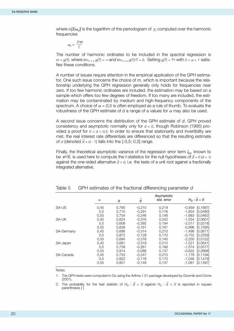
A number of issues require attention in the empirical application of the GPH estima-tor. One such issue concerns the choice of m, which is important because the rela-tionship underlying the GPH regression generally only holds for frequencies nearzero. If too few harmonic ordinates are included, the estimation may be based on asample which offers too few degrees of freedom. If too many are included, the esti-mation may be contaminated by medium and high-frequency components of thespectrum. A choice of � = 0,5 is often employed as a rule of thumb. To evaluate therobustness of the GPH estimate of d a range of a values for � may also be used.

A second issue concerns the distribution of the GPH estimate of d. GPH provedconsistency and asymptotic normality only for d < 0, though Robinson (1995) pro-vided a proof for 0 < d < 0,5. In order to ensure that stationarity and invertibility aremet, the real interest rate differentials are differenced so that the resulting estimateof d (denoted d = d - 1) falls into the [-0,5; 0,5] range.

Finally, the theoretical asymptotic variance of the regression error term �s, known to be �2/6, is used here to compute the t-statistics for the null hypotheses of d = 0 (d = 1)against the one-sided alternative d < 0, i.e. the tests of a unit root against a fractionallyintegrated alternative.


SA RESERVE BANK

Table 5 GPH estimates of the fractional differencing parameter d

~Asymptotic ~

� d d std. error H0 : d = 0

SA-US 0,45 0,790 -0,210 0,219 -0,959 [0,1687]0,5 0,710 -0,291 0,176 -1,654 [0,0490]

0,55 0,754 -0,246 0,146 -1,683 [0,0462]SA-UK 0,45 0,624 -0,376 0,242 -1,554 [0,0601]

0,5 0,608 -0,392 0,194 -2,017 [0,0218]0,55 0,839 -0,161 0,161 -0,996 [0,1595]

SA-Germany 0,45 0,686 -0,314 0,210 -1,498 [0,0671]0,5 0,872 -0,128 0,170 -0,752 [0,2259]

0,55 0,684 -0,316 0,140 -2,250 [0,0122]SA-Japan 0,45 0,681 -0,319 0,210 -1,521 [0,0641]

0,5 0,739 -0,261 0,166 -1,574 [0,0577]0,55 0,914 -0,086 0,137 -0,622 [0,2668]

SA-Canada 0,45 0,753 -0,247 0,210 -1,178 [0,1194]0,5 0,822 -0,178 0,170 -1,046 [0,1479]

0,55 0,851 -0,149 0,137 -1,081 [0,1397]

Notes

1. The GPH tests were computed in Ox using the Arfima 1.01 package developed by Doornik and Ooms(2001).

~ ~2. The probability for the test statistic of H0 : d = 0 against H0 : d < 0 is reported in square

parentheses [ ].

~

~

~

The GPH estimates of d (corresponding to d = 1 + d) for the bilateral real interestrate differentials between South Africa and each of the USA, UK, Germany, Japanand Canada are reported in Table 5. Choosing m = T0,45, T0,5, T0,55, these estimates ofd lie between 0,608 and 0,914 (for m = T0,5 the estimates of d are between 0,608 and0,872). The tests of the unit root null hypothesis against a one-sided fractionally inte-grated alternative provide evidence that the real interest rate differential is fractionallyintegrated in all cases except for the SA-Canada differential (for all other differentials,2 of the 3 tests reported reject at the 10 per cent level, i.e. the probability reportedin square parentheses [ ] is < 0,1).

The evidence provided by these tests therefore supports the view that real interestrates in South Africa are linked to those in the US, UK, Germany and Japan in thatthe interest rate differentials with these countries are mean reverting. This is consis-tent with the existence of real interest parity as a long-run equilibrium condition. Sincethe differentials exhibit I(d) behaviour, however, their dynamics are persistent, andreversion to real interest parity may be rather slow.16 It is for this reason that traditionalI(0)/I(1) unit root tests are often unable to capture this reversion.

7. Implications and conclusions

There is no simple way of determining precisely the appropriate level of real interestrates. In an open economy they must have some reference to international levelsalthough the evidence presented here for South Africa suggests that the links are notstrong, particularly in the short run. It appears that the stance of monetary policy inSouth Africa has resulted in short-term real interest rates that are higher than the inter-national average. However, the differential declined in the course of 2000, although therecent declines in official rates internationally would have reversed this trend.

From a policy perspective, the current situation cannot be seen in isolation from thecurrent monetary policy framework and the level of the inflation rate relative to thetarget. A simple Taylor rule would suggest that the further the current rate is from thetarget (and the higher real economic activity is), the higher the real interest rateshould be. When the current inflation rate exceeds the target, the nominal rate hasto be raised by more than the expected acceleration in inflation in order to make theincrease in the nominal interest rate equivalent to an increase in the real interest rate(subject to the degree of deviation from potential output). Countries that are at oraround their inflation target can therefore have lower real rates and have more flexi-bility to adjust rates. It is significant for example that South Africa’s real rates are similar to those of Mexico where the inflation target is still to be achieved. Therefore,although real rates have come down from the highs of 1998, current rates reflect toa certain extent the Reserve Bank’s overriding commitment to the inflation target.

Finally, can the Reserve Bank reduce the cost of capital by engineering artificially lowinterest rates? Any attempt by the Reserve Bank to artificially reduce the cost of cap-ital may succeed in the short run but cannot be sustained, particularly in the face ofincreased capital mobility. The ultimate effect of excessively low nominal interestrates is to raise inflation and long-term interest rates. The short-term benefit of lowshort-term real interest rates would be offset by the longer-term costs of higher infla-tion. The experiences of countries such as Canada, New Zealand and Australia haveshown that real interest rates can be maintained at lower levels once the inflation tar-gets have been achieved. However these countries did experience higher short-termreal rates in the phase of adjustment of the inflation rate to the target.

21

SA RESERVE BANK


~

16 Further evidence of closerlinkages over time betweenSouth African and internationalreal interest rates was obtainedfrom running recursive GPHestimates of d on increasingwindows (samples) of the set ofreal interest rate differentials.Declining estimated values of d,which suggest an increase inthe degree of mean reversionfor the differential over time,were revealed for South Africa’sdifferentials with the US, UKand Japan. The estimated val-ues of d for the differentials withGermany and Canada do notappear to trend downward over time.

Appendix 1: The data

Short-term and long-term real interest rates were calculated for various countriesusing inflation and interest rate data from the International Financial Statistics CD-ROM of the IMF (March, 2001). Short-term real interest rates were calculated at theannual and monthly frequencies, and long-term real interest rates were calculated atthe annual frequency.

Price inflation was measured using changes in consumer price indices (CPIs) (IFSline 64). The short-term nominal interest rates were proxied using discount rates(end of period, IFS line 60) where available (money-market rates were used whenthis was not the case; IFS line 60b). Long-term government bonds (IFS line 61) wereused for the long-term rates.

The table below provides details of the data sample periods for each country for theannual (short-term and long-term) conventional real interest rates used in Figures 2and 3, and for monthly conventional real interest rates which are used in the empirical work in Section 6.

The following dating conventions were employed to construct the real interest ratesdiscussed in the text: The conventional short-term (long-term) real interest rate wascalculated at the annual frequency by subtracting the inflation rate in the previousyear from the current annualised discount (long-term government bond) rate. At themonthly frequency, the conventional short-term real interest rate is the annualisednominal rate in the current period less the year-on-year inflation rate in the preceding period [i.e ((CPIt - CPIt-12)/ CPIt-12) *100].

Ex post and ex ante short-term real interest rates were also calculated (Figure 1). Theex post short-term real interest rate at the annual frequency is the current annualiseddiscount rate less the inflation rate realised in the subsequent year. At the monthlyfrequency, this rate is the annualised nominal rate in the current month less the year-on-year inflation rate realised in the subsequent period [i.e ((CPIt+12 - CPIt)/ CPIt) *100].The ex ante short-term real interest rate was calculated using annual data by sub-tracting the annualised inflation rate expected over the subsequent year from thecurrent annualised discount rate. As proxy for expected inflation, a Hodrick-Prescottfilter was used to calculate the low frequency component of the actual year-on-year


SA RESERVE BANK

Table: Data sample periods

Annual data: Monthly data:Short-term Long-term

Country rate rate Short-term rate

Australia 1970-2000 1950-2000 –Canada 1950-2000 1950-2000 Jan 1957 – Dec 2000Chile 1977-2000 – –France 1950-2000 1950-2000 –Germany 1950-2000 1956-2000 Jan 1960 – March 2001Japan 1950-2000 1966-2000 Jan 1957 – March 2001Mexico 1978-2000 – –New Zealand 1950-2000 1950-2000 –South Africa 1950-2000 1950-2000 Jan 1957 – March 2001UK 1969-2000 1950-2000 Jan 1972 – Jan 2001USA 1950-2000 1954-2000 Jan 1964 – March 2001

inflation series (a smoothing parameter of 100 was imposed on the annual data). Asan alternative, a three-year backward-weighted average was also employed andreported in Figure 1 (inflation in the current period t was given a weight of 0,5, thatin t-1 a weight of 0,3, and that in t-2 a weight of 0,2).

Appendix 2: Unit root tests

This appendix briefly sets out the two tests used in Section 6.2 of the paper. Thefirst is the “generalised least squares” (GLS) version of the standard ADF test intro-duced by Elliott, Rothemberg and Stock (1996). This DF-GLS test uses the localGLS-demeaned (DF-GLS�) or the local GLS-demeaned and detrended series (DF-GLS�) to compute the t-statistic on the coefficient � (� = � - 1) in the regressionequation

_ _ n _∆ yt = � yt-1 + �j ∆yt-j + et (A2.1)

j=1

_where yt is the detrended and/or demeaned transform of yt and et is white noise. Withappropriate critical values, this t-statistic is used to test the null hypothesis of a single unit root (� = 1) against the local alternative

_� = 1 +

_c /T (where T is the

sample size, _c is some constant).

_The first step in calculating the DF-GLS tests is therefore to generate the series yt.Consider firstly the demeaned and detrended case. Setting zt = (1,t), �GLS is estimatedby GLS, i.e. from the OLS regression of [y1, y2 -

_� y1, ... , yT -

_� yT-1] onto [z1, z2 -

_� z1, ... ,

zT - �zT-1]. The demeaned and detrended yt is then calculated as

– – yt = yt - zt �GLS (A2.2)

The series yt is demeaned in similar fashion, with the regressor t being excluded fromzt. Following Elliot, Rothemberg and Stock (1996),

_c is set equal to -7 in generating

the demeaned series and equal to -13,5 in the demeaned and detrended case.

Note that the test statistic in the demeaned case has the same distribution as theADF test with no deterministic elements included. Approximate finite sample criticalvalues for the demeaned and detrended case are provided by Elliott, Rothembergand Stock (1996, Table 1), whereas Cheung and Lai (1995) estimate response surfaces for the tests which provide the lag-adjusted finite sample critical valuesused in this study.17

The second test is the KPSS test of Kwiatkowski et al. (1992), which uses a para-meterisation that allows a null hypothesis of stationarity to be tested. Treating theobserved series yt as the sum of a deterministic component f(t), a stochastic trend rt,and a stationary residual �t, the components model

yt = f(t) + rt + �t (A2.3)

is obtained where f(t) = a constant (or a constant and a trend), rt = rt-1 + ut , ut ~ iid(0,�2u ),

and �t is stationary and independent of ut at all lags.

23

SA RESERVE BANK


17 In practice, the lag order nin (A2.1) is not known, and hasto be selected. This is an impor-tant decision; choosing n toosmall results in size distortions,but selecting n too large willdecrease the power of the testas degrees of freedom are lost.Theoretical and simulation evidence suggest that the selection of the lag length nshould be undertaken usingpretest data-based model seletion procedures. Simulationresults in Hall (1994), for exam-ple, suggest that estimating nfrom the data may result in again in power over fixing n at arelatively long length. In thisstudy, the lag length n wasselected using the informationcriterion proposed by Schwarz(1978). This chooses n by min-imising T In�2+CT over a rangeof lag orders, where �2 is themaximum likelihood estimate ofthe variance �2 in the relevantregression equation and CTequals k(InT). All parameters inthe regression equation areincluded in the computation ofthe information criterion, so k isequal to n + 1 (no deterministiccomponent), n + 2 (demeanedtest), or n + 3 (demeaned anddetrended test).

~~

Since the stochastic trend rt is annihilated when the variance of ut = 0, and since �t isstationary, the null hypothesis of stationarity (trend stationarity when f(t) = a constantand a trend) is

H0 : � 2 = 0 . (A2.4)u

The KPSS test is conducted by regressing yt on a constant (or a constant and a trend),denoting the residuals e = [e1 , …, eT ] / and constructing the KPSS statistic �

^ T� = T-2 S

t2 / S2 (l) (A2.5)

t=1

where St is the partial sum

tSt = e j (A2.6)

j=1

and S2(l) is a heteroscedasticity and autocorrelation consistent variance estimatorgiven by

T l TS2(l) = T-1 e

t2 + 2T-1 w(s,l) etet-s . (A2.7)

t=1 s=1 t=s+1

Here w(s,l) is an optimal weighting function that corresponds to the choice of spec-tral window. We use a Bartlett window w(s,l) = 1 – s /(l+1), as suggested by KPSS. Thetruncation lag l was selected using the l8 rule of KPSS (1992), which sets l = INT{8*(T/100)^(1/4)}. Critical values were taken from KPSS (1992, Table 1).


SA RESERVE BANK

References

Allsopp, C. and Glyn, A. 1999. The assessment: real interest rates, Oxford Reviewof Economic Policy, 15(2), p 1-16.

Amano, A. A. and van Norden, S. 1992. Unit root tests and the burden of proof,mimeo.

Atkinson, P. and Chouraqui, J-C. 1985. The origins of high real interest rates, OECDEconomic Studies, No 5 (Autumn).

Baillie, R. T. 1996. Long memory processes and fractional integration in economet-rics, Journal of Econometrics, 73, p 5-59.

Barro, R. J. and Sala-i-Martin, X. 1990. World real interest rates. In O Blanchard andS Fischer (eds) NBER Macroeconomics Annual, Cambridge: MIT Press.

Begum, J. 1998. Correlations between Real Interest Rates and Output in a DynamicInternational Model: Evidence from G-7 Countries, IMF Working Paper WP/98/179.

Blanchard, O. and Summers, L. H. 1984. Perspectives on high real world interestrates, Brookings Papers in Economic Activity, p 273-334 (including comments anddiscussion).

Breedon, F., Henry, B. and Williams, G. 1999. Long-term real interest rates: evidenceon the global capital market, Oxford Review of Economic Policy, 15(2), p 128-42.

Chadha, J. S. and Dimsdale, N. H. 1999. A long view of real rates, Oxford Reviewof Economic Policy, 15(2), p 17-45.

Cheung, Y. W. and Chinn, M. D. 1994. Further investigation of the uncertain unit rootin GNP, Department of Economics Working Paper No 288, University of CaliforniaSanta Cruz, April.

Cheung, Y. W. and Lai, K. S. 1995. Lag order and critical values of a modifiedDickey-Fuller test, Oxford Bulletin of Economics and Statistics, 57(3), p 411-19.

Cumby, R. and Mishkin, F. 1986. The international linkage of real interest rates: theEurope – US connection, Journal of International Money and Finance, p 845-55.

Diebold, F. X. and Rudebusch, G. D. 1991. On the power of Dickey-Fuller testsagainst fractional alternatives, Economics Letters, 35, p 155-60.

Doornik, J. A. and Ooms, M. 2001. A package for estimating, forecasting and sim-ulating Arfima models: Arfima package 1.01 for Ox, Discussion paper, Oxford:Nuffield College.

Elliott, G., Rothemberg, T. J. and Stock, J. H. 1996. Efficient tests for an autore-gressive unit root, Econometrica, 64, p 813-36.

Fama, E. F. 1975. Short term interest rates as predictors of inflation, AmericanEconomic Review, 65, p 269-82.

25

SA RESERVE BANK


Felmingham, B., Qing, Z and Healy, T. 2000. The interdependence of Australian andforeign real interest rates, The Economic Record, 76(233), p 163-71.

Fisher, I. 1930. The Theory of Interest, New York: Macmillan.

Ford, R. and Laxton, D. 1999. World public debt and real interest rates, OxfordReview of Economic Policy, 15(2), p 77-94.

Fujii, E. and Chinn, M. D. 2000. Fin de siecle real interest parity, NBER WorkingPaper 7880, National Bureau of Economic Research, Cambridge, September.

Garcia, R. and Perron, P. 1996. An analysis of the real interest rate under regimeshifts, Review of Economics and Statistics, p 111-25.

Geweke, J. and Porter-Hudak, S. 1983. The estimation and application of longmemory time series models, Journal of Time Series Analysis, 4, p 221-238.

Granger, C. W. J. and Joyeux, R. 1980. An introduction to long memory time seriesmodels and fractional differencing, Journal of Time Series Analysis, 1, p 15-39.

Hall, A. 1994. Testing for a unit root in time series with pretest data-based modelselection, Journal of Business and Economic Statistics, 12(2), p 461-70.

Helbling, T. and Wescott, R. 1995. The global real interest rate, IMF Staff Studies forthe World Economic Outlook, p 28–50.

Hosking, J. R. M. 1981. Fractional differencing, Biometrika, 68, p 165-76.

Howe, H. and Pigott, C. 1991. Determinants of long-term interest rates: an empiri-cal study of several industrial countries, Federal Reserve Bank of New York QuarterlyReview, 16, Winter (1991/92), p 12-28.

Huizinga, J. and Mishkin, F. 1986. Monetary policy regime shifts and the unusualbehavior of real interest rates, Carnegie-Rochester Conference Series on PublicPolicy, 24, p 231-74.

Jenkinson, T. 1999. Real interest rates and the cost of capital, Oxford Review ofEconomic Policy, 15(2), p 114-27.

Kaminsky, G. L. and Leiderman, L. 1996. High real interest rates in the aftermath ofdisinflation: is it a lack of credibility? International Finance Discussion Paper No 543,Board of Governors of the Federal Reserve System, March.

Kwiatkowski, D., Phillips, P. C. B., Schmidt, P. and Shin, Y. 1992. Testing the nullhypothesis of stationarity against the alternative of a unit root: how sure are we thateconomic time series have a unit root? Journal of Econometrics, 54, p 159-78.

Lai, K. S. 1997. Long-term persistence in the real interest rate: some evidence of afractional unit root, International Journal of Finance and Economics, 2, p 225-35.

Lee, D. and Schmidt, P. 1996. On the power of the KPSS test of stationarity againstfractionally-integrated alternatives, Journal of Econometrics, 73, p 285-302.


SA RESERVE BANK

Levy, A. and Panetta, F. 1996. The main trends of real interest rates (1960-1994). In C Pierluigi, and G Nardozzi. The high price of money: an interpretation of worldinterest rates, Oxford: Clarendon Press.

Mishkin, F. S. 1988. Understanding real interest rates, American Journal ofAgricultural Economics, 70, p 1064-72.

Moosa, I. A. and Bhatti, R. H. 1996. Some evidence on mean reversion in ex antereal interest rates, Scottish Journal of Political Economy, 43(2), p 177-91.

Orr, A., Edey, M. and Kennedy, M. 1995. Real long-term interest rates: the evidencefrom pooled-time-series, OECD Economic Studies No 25, p 75-107.

Pain, D. and Thomas, R. 1997. Real interest rate linkages: testing for commontrends and cycles, Bank of England Working Paper No 65, Bank of England, July.

Phillips, P. C. B. 1998. Econometric analysis of Fisher’s equation, CowlesFoundation Discussion Paper No 1180, Yale University, 14 May.(http://cowles.econ.yale.edu).

Robinson, P. 1994. Time series with strong dependence, Advances inEconometrics, 6th World Congress, 1, CUP: Cambridge, p 47-96.

Robinson, P. 1995. Log-periodogram regression of time series with long rangedependence, Annals of Statistics, 23, p 1048-72.

Rose, A. K. 1988. Is the real interest rate stable?, Journal of Finance, 43, p 1095-112.

Schwarz, G. 1978. Estimating the dimension of a model, Annals of Statistics, 6, p461-64.

Scott, M. 1993. Real interest rates: past and future, National Institute EconomicReview, February, p 54-69.

Smith, J. C. 1986. Real interest rates, saving and investment, The WarwickEconomics Research Paper Series No 454, University of Warwick, March.

Stock, J. H. 1994. Unit roots, structural breaks and trends. In R Engle and DMcFadden (eds) Handbook of Econometrics, vol. IV, North-Holland: Amsterdam, p 2739-841.

27

SA RESERVE BANK


Previous Occasional Papers

Occasional Paper No. 1, December 1990; The optimal allocation of savings in theSouth African economy and the role of monetary policy by J A Lombard and J P vanden Heever.

Occasional Paper No. 2, December 1990; Notes on oil, gold and inflation.

Occasional Paper No. 3, January 1991; South Africa’s balance of payments: Sources,methods and reliability by E.J. van der Merwe and M.C. Bester.

Occasional Paper No. 4, July 1991; South Africa’s public-sector accounts 1973to 1990.

Geleentheidspublikasie no. 5, September 1991; Suid-Afrika se nasionale rekeninge,1946 tot 1990.

Occasional Paper No. 6, May 1993; Is South Africa in a debt trap? by E J vander Merwe.

Occasional Paper No. 7, April 1995; The framework of the public sector equations inthe South African Reserve Bank’s econometric model by M M Smal.

Occasional Paper No. 8, June 1995; The compilation and importance of householddebt in South Africa by B.E. van der Walt and J W Prinsloo.

Occasional Paper No. 9, March 1996; Exchange rate management policies in SouthAfrica: Recent experience and prospects by E J van der Merwe.

Occasional Paper No. 10, May 1996; The forecast performance of alternative models ofinflation by C J Pretorius and T N Janse van Rensburg.

Occasional Paper No. 11, July 1998; The framework of the monetary block’s equa-tions in the South African Reserve Bank econometric model by S de Jager.

Occasional Paper No. 12, August 1998; The influence of socio-political developmentson banks in South Africa, 1992-1997 by S J van der Walt.

Occasional Paper No. 13, September 1999; The forward rate as an optimal predictor ofthe future spot rate in South Africa: An econometric analysis by G R Wesso.

Occasional Paper No. 14, November 2000; The saving behaviour of the South Africaneconomy by J W Prinsloo.

Occasional Paper No. 15, July 2001; Capital controls and the volatility of South Africanexchange rates by G N Farrell.

Occasional Paper No. 16, September 2001; The monetary transmission mechanismin South Africa by M M Smal and S de Jager.


SA RESERVE BANK

south african real interest rates in comparative ... and publications/attachments... · south...

Documents