Sovereign Debt and Systemic Risk

Christophe Hurlin Alexandra Popescu

Camelia Turcu

University of Orleans

May 13, 2013

Preliminary version. Please do not cite.

Abstract

Within the framework of the current crisis, it seems that an evaluation of systemic

risk in the sovereign sector is an urgent matter that needs to be tackled. Thus, we

propose an application of the systemic risk measures on macroeconomic data related

to sovereign debt. To the best of our knowledge, the systemic risk concept was applied

only to the stock market so as to measure the riskiness of financial institutions. We

propose in this paper to transpose the notion of systemic risk to the sovereign debt

crisis in order to determine which are the most systemically important countries in the

Euro Area. A country becomes systemically important when its debt is no longer sus-

tainable and default on repaying its debt would cause significant adverse consequences

for the entire system. As our aim is to identify the contribution of each country to

the system’s default, we use a Sovereign Systemic Risk measure (SsRisk) based on the

Marginal Expected Shortfall (MES) propose by Brownlees and Engle (2011) and on

the budgetary constraint of the analyzed countries. The MES is estimated using a Dy-

namic Conditional Correlation model (DCC). To compute our measure, we use daily

data on the Euro zone countries on the period 2000-2011 related to the government

bonds yields 10Y and quaterly macroeconomic data on countries sovereign debts. The

main results of our estimations allow us to perform comparisons in terms of countries

riskiness within the Eurozone.

Keywords: Systemic risk, sovereign debt, debt crisis.

JEL classification: G28, H63.

1

1 Introduction

What would be the consequences of a potential default of Greece, Spain, Ireland or France on

the ability of other European countries to finance their debt? Do European countries have

an incentive to save Greece from default? These issues are crucial, but economists have no

clear answer to these questions. Why? Simply because we have not observed in the recent

past a sovereign default of a major European country. Thus, we cannot scientifically assess

the consequences of such a situation.

However, these issues and limitations are largely similar to those we face when evaluat-

ing the systemic risk contribution of financial institutions (Acharya et al. 2010). Even if a

financial institution has never experienced bankruptcy (for example, Lehman before 2008),

the impact of such a potential event on the stability of the whole financial system is central

to this literature. Within this framework, one of the most popular systemic risk measures

proposed thus far is the Systemic Risk index (SRISK hereafter) recently proposed by Brown-

lees and Engle (2011). The SRISK measures the part of the total expected system capital

shortfall in a crisis that is due to a particular financial institution. The firms with the largest

capital shortfall are the greatest contributors to the crisis and are the institutions considered

as most systemically risky. Hence, large expected capital shortage in a crisis does not only

capture individual firm vulnerability, but also systemic risk. The SRISK is based on two

elements: (i) the Marginal Expected Shortfall (MES) defined as the expected equity loss of

a firm when the overall market declines beyond a given threshold over a given time horizon

and (ii) the leverage of the firm.

Our goal is to transpose these systemic risk measures initially developed for the market

risk to the sovereign debt risk. Hence, we aim to determine what are the European countries

that contribute the most to the global systemic risk of the Euro Area. To the best of our

knowledge, this is the first attempt to propose a systemic sovereign debt risk measure.

In this perspective, a country is systemically important when its debt is no longer sus-

tainable and default on repaying this debt would cause significant adverse consequences for

the entire system. A default is likely to appear whenever the yield is so high that it becomes

impossible for the country to raise the necessary funds to repay its outstanding obligations.

Correspondingly, the MES can be defined as the expected increase in a particular govern-

ment bond yield when the overall (European) government bonds market is beyond a given

threshold over a given time horizon, i.e. when interest rates exceed a given threshold.

Based on the government budget constraint, we derive a new concept of SsRISK (Systemic

Sovereign Risk) index that depends on the MES and on the specificities of each country in the

Eurozone, like the amount of public debt, its primary deficit and its growth rate. The SsRISK

2

allows us identify systemically important countries, that is the countries that contribute the

most to systemic risk in the Euro area.

The rest of the paper is structured as follows. Section 2 presents the the theoretic frame-

work which allows us to derive our risk measure. In section 3, we describe the econometric

methodology employed to compute them. In section 4, based on the two measures, we per-

form an analysis of systemic risk in the Euro area and determine which countries present

the most risk to the system. Section 4 concludes.

2 Systemic Sovereign Risk: A Financial Approach

Our aim is to evaluate the expected financing requirements of Eurozone countries during a

debt crisis which takes place at European level. On this basis, we further determine which

countries contribute the most to systemic sovereign risk. The approach we use is similar

to the one applied to financial institutions. As defined by Brownlees and Engle (2011), the

systemic risk of a financial institution is perceived as “its contribution to the total capital

shortfall of the financial system that can be expected in a future crisis”. The idea underlying

this definition is that, when the financial system undergoes a crisis, the failure of a financial

firm - due to large capital losses - imposes a negative externality not only on the financial

sector, but on the real economy as well. Thus, the higher the capital shortfall, the greater

the firm’s contribution to systemic risk.

In this paper, we apply the same framework in order to assess the financing requirements

of European countries. For a country, systemic risk is seen as a situation where the default on

repaying sovereign debt would cause significant adverse consequences for the entire system.

A default is likely to appear whenever the yield is so high that it becomes impossible for the

country to raise the necessary funds to repay its outstanding obligations1. Thus, a country

is systemically risky if it is likely for it to face large capital requirements at a time when the

whole system is under stress.

In order to identify and measure the financing requirements of a country, we start from

the standard budgetary constraint equation2. Let Yit be the real GDP of country i at time t

and let Bit be the real value of public debt. The government budget constraint combines the

nominal interest rate rit, net inflation πit, net growth in real GDP git (between t− 1 and t),

and the primary deficit defit in order to obtain the evolution of the government debt-GDP

1 We suppose that the country is unable to raise funds in any other way (i.e. seigneurage, increase intaxes, reduction of public investment).

2 In the case of financial institutions, the risk measure is derived frosm a Basel-type regulatory constraint.

3

ratio:Bit

Yit= (rit − πit − git)

Bi,t−1

Yi,t−1+defitYit

+Bi,t−1

Yi,t−1. (1)

The nominal return rit and the real stock of debt Bit in equation (1) are averages across

terms to maturity3. The increase in the real debt stock at time t for country i can be

expressed as follows:

Bit −Bi,t−1 = [(git + 1) (1 + rit − πit − git)− 1]×Bi,t−1 + defit (2)

From this standard budgetary constraint, we derive the definition of the expected financing

requirements4, that we call debt shortage.

Definition. The debt shortage represents the expected increase in debt of country i at date

t conditional on the emergence of a European debt crisis:

DSi,t−1 = Et−1 (Bit −Bi,t−1|Crisis) (3)

The increase in debt represents a rise in the financing requirements of the country. To

deal with this need of funding, the government will have to issue new debt at a yield rate

imposed by the market. The concept of debt shortage is similar to that of an institution’s

capital shortfall used by Brownlees and Engle (2011), i.e. the capital that a financial firm

would need to raise if another financial crisis developed. Considering the above definition

and the result in equation (3), we obtain the following expression for the debt shortage of a

country:

DSi,t−1 = Et−1 ( [(git + 1) (1 + rit − πit − git)− 1]×Bi,t−1 + defit|Crisis) . (4)

We consider the crisis event as the situation where the whole area - the Euro area in our

case - faces a difficulty to raise funds, i.e. high bond rates, and to finance the mutualized debt

defined as the sum of individual debts of all countries under analysis. Under the framework

of Brownlees and Engle (2011), the systemic event is defined as a drop of the market index

below a certain threshold, over a given period of time. Two differences can be identified

when trying to apply the same logic to sovereigns. First of all, as Eurobonds are not yet

implemented, we have no global index for the area. To define a crisis situation, we therefore

have to build a virtual index that we compute as an average of each member state interest

rate weighted by its public debt. Let us define the nominal bond rate of the market rmt as

3 See Hall and Sargent (2010) for different maturity structures of debt.4 For a complete development of the model refer to the appendix.

4

the virtual rate that should be applied to the mutualized debt in order to equalizes the sum

of interest paid on the N individual debts:

rmt

N∑i=1

Bit =N∑i=1

ritBit (5)

where m stands for the market and i for the country.

At this point, we could define a European debt crisis as an increase in this yield index

over a certain threshold5. Nevertheless, a second problem arises. The dynamics of sovereign

bond yields are not stationary, therefore the index will also be integrated of order one. In this

case, the probability that the yield index becomes greater than a fixed threshold increases

with time. To solve this issue, we model government bond yields as random walks:

rjt = rj,t−1 + zjt with j = {i,m} (6)

and we define the crisis event as an abnormal surprise observed in the European yield index.

Definition. The crisis event at the European level is defined as the occurrence of an unex-

pected major positive innovation in the European bond yield index:

Crisis : zmt > C (7)

The threshold value C can be either a conditional or an unconditional value. Depending

on the choice of this value, the probability of observing the systemic event is constant or

time-varying. We choose C to be the historical Value-at-Risk (V aR) at a 5% confidence

level. As zmt is modeled as a Garch process, Pr(zmt > C) will be time dependant.

Having defined the conditioning event and assuming that git and defit are predetermined,

we can now derive the formula for the debt shortage of a country:

DSit = [(git + 1) (1 + Et−1 (rit|Crisis)− Et−1 (πit|Crisis)− git)− 1]×Bi,t−1 + defit

= [(git + 1) (1 + Et−1 (ri,t−1 + zit| zmt > C)− Et−1 (πit|Crisis)− git)− 1]×Bi,t−1 + defit.

(8)

DSit represents the capital that a country would need to raise, if the European bond

market experienced a crisis. Such a measure helps us to answer questions like what would be

5 The sign of our inequality is reversed with respect to Brownlees and Engle’s approach, as in our case,systemic events are situated in the right tail of the yields distribution.

5

the expected financing requirements of Greece or Italy when the European market is faced

with an unexpected increase in its yield index. This financing requirement depends both

on the structural factors of each country - primary deficit, public debt level, inflation and

growth rate - and on the spillover effects captured by the expectation term on the yields in

equation (8). This term gives the expectation of the bond rate of one country, conditional

on the market being taken by surprise, and corresponds to the marginal expected shortfall

(MES) used in the financial approach.

A large debt shortfall in the Euro area will cause a real crisis. The countries with the

highest debt shortfall are the greatest contributors to systemic risk, thus are the countries

considered as most systemically risky. Hence, large expected debt shortage in a generalized

debt crisis does not just capture individual country vulnerability, but also systemic risk. As

Brownlees and Engle (2011), we further use this measure to compute a systemic sovereign

risk index (SsRISK) that will help us to classify countries by their systemic importance.

Definition. We define the systemic sovereign risk index of government i as:

SsRISKit = max (0, DSit) (9)

We take the maximum between 0 and DSit as we are only interested in positive financing

requirements. A negative DSit means either that the individual yield of a country is nega-

tively correlated with the market yield or that the country does not need structural financing

as it is characterized by high growth, low deficit or low debt level. The percentage version

of the index gives us the contribution of a country to systemic risk:

SsRISK%it = SsRISKit/N∑i=1

SsRISKit (10)

Hence, the SsRISK% index measures the portion of the total expected system debt short-

age in a crisis that is due to government i. Our key assumption is that debt shortages of a

given country impose external costs on the other countries when they occur during a period

of distress for the whole system. These costs can be viewed as externalities that are partic-

ularly severe when the entire Euro area faces difficulties to issue debt. When the economy

is in a downturn, the default of a government has even harsher consequences than in normal

times, on both the financial and the real sectors. Thus the shortage of capital is dangerous

for one country and for its bondholders, but it is dangerous for the global system (Euro

area) if it occurs just when the rest of (European) countries also need funds to finance their

deficits.

6

3 Methodology

Computing the debt shortage of one country requires data on its public debt, primary deficit

and growth rate, but also requires estimating the two expectation terms in equation (8).

For the expected value of the country’s yield conditional on the emergence of a European

debt crisis, the methodology applied makes use of a Dynamic Conditional Correlation model,

whereas for the expected inflation conditional on the same systemic event, a historical ap-

proach is being used. Details on both this methodologies are provided below.

3.1 The Dynamic Approach

To estimate the dependence between bond yields of countries and the innovations of the

market yield, Et−1 (rit|zmt > C), we start from a simple bivariate process where innovations

{zit} and {zmt} are expressed as:

zit = σitεit = σit

(ρitεmt +

√1− ρ2itξit

)zmt = σmtεmt

(11)

with σit and σmt the volatilities of the bond yields of each country i and of the market, ρit the

correlation between the market and country i. Moreover the disturbances are independent

and identically distributed over time:

zt = (zmt, zit) ∼ F (12)

so that Et−1(zt) = 0 and Et−1(ztz′t) = Ht. The covariance matrix is written as:

Ht =

σit ρitσitσmt

ρitσitσmt σmt

(13)

Using this framework, we compute the conditional expectation of bond yields as follows:

Et−1(rit | zmt > C) = Et−1(ri,t−1 + zit | zmt > C)

= ri,t−1 + σitEt−1(εit | εmt > Cσmt

)

= ri,t−1 + σitEt−1(ρitεmt +√

1− ρ2itξit | εmt > Cσmt

)

= ri,t−1 + σitρitEt−1(εmt | εmt > Cσmt

) + σit√

1− ρ2itEt−1(ξit | εmt > Cσmt

).

(14)

This expectation is, hence, a function of the country’s bond yield volatility, σit, the

7

correlation between the yield of the country and the market yield, ρit, and the comovement

in the tails of distribution. Individual volatilities and correlations are estimated with a DCC

model6, whereas the tail expectations are computed through a non parametric approach.

3.1.1 The DCC model

A bivariate DCC is used to model the volatility and the correlations between the bond yield

index and the yields of each country i. The conditional covariance matrix is decomposed as

follows:

Ht = DtRtDt,(15)

where Dt =

σit 0

0 σmt

represents a 2 by 2 diagonal matrix of volatilities and where Rt = 1 ρimt

ρimt 1

denotes the time varying correlation matrix.

As usual, a two step approach is used to estimate this model. In the first stage, a

univariate Garch(1,1) is considered for each of the eleven countries and for the market index.

The conditional variance of this model class is given by:

σ2it = ωi + αiz

2i,t−1 + βiσ

2i,t−1, (16)

σ2mt = ωm + αmz

2m,t−1 + βmσ

2m,t−1, (17)

The model parameters are estimated using the Quasi Maximum Likelihood approach (QML).

In the second stage, we express the dynamic conditional correlation matrix as:

Rt = diag(Qt)−1/2Qtdiag(Qt)

−1/2, (18)

where Qt is the pseudo conditional correlation matrix of the returns standardized by their

conditional standard deviation obtained previously, ε∗t = zitσit

. To compute Qt, we introduce

these standardized returns into a DCC(1,1) model:

Qt = (1− αC − βC)S + αCε∗t−1ε

∗′t−1 + βCQt−1, (19)

6 Arch effects were found for all the series in our sample.

8

where ε∗t is the vector of standardized returns, S is the unconditional covariance matrix of

ε∗t and αC and βC the DCC parameters to be estimated.

The conditions for the positive definiteness of Ht can be found in Engle and Sheppard

(2001) and Brownlees and Engle (2011). The former also provides consistency and asymp-

totic normality conditions based on the work of Newey and McFadden (1994). In order to

obtain robust standard errors, the covariance matrix is computed as A−1BA−1T−1, where A

represents the analytic hessian and B the covariance of the scores.

3.1.2 Non parametric estimation of tail expectations

In order to compute the expectation of the bond yield conditional on a crisis event, the final

elements needed are tail expectations. For obtaining these values, we use a non parametric

kernel estimation. The methodology applied here follows Scaillet (2005), with two notable

differences. First, in our case, the conditioning with respect to past information is not

necessary since we apply the formula on standardized residuals that are independent and

identically distributed. Second, the sign in the conditioning event is reversed. Let

Φ(x) =

∫ x/h

−∞k(u) du, (20)

where k(u) is the normal kernel function and h is a positive bandwidth. Then, the tail

expectations are:

Eh(εmt|εmt > κ) =

T∑t=1

εmt(1− Φ(κ−εmt

h))

T∑t=1

(1− Φ(κ−εmt

h)) , (21)

Eh(ξmt|εmt > κ) =

T∑t=1

ξmt(1− Φ(κ−εmt

h))

T∑t=1

(1− Φ(κ−εmt

h)) , (22)

where h is the bandwidth parameter, κ is the cutoff point and Φ(·) represents the normal

cumulative distribution function 7. For the determination of the bandwidth, we follow Scaillet

(2005) and fix its value at T−1/5 times the empirical standard deviation, equal to 1 in our

case. The cutoff, κ, is given by C/σmt.

7 For more details on the formulas, see appendix C.

9

3.2 The Historical Approach

The second expectation term concerns the value of inflation given the occurrence of the

systemic event. As inflation series do not present arch effects, the dynamic estimation is

not appropriate. Hence, a historical approach is preferred when computing this conditional

expectation. This methodology was first proposed by Acharya et al. (2010), and reconsidered

afterwards by Brownlees and Engle (2011), in their computations of the MES. The historical

rolling MES, as defined by the latter, is the average loss for a firm when the market returns

are lower than a certain negative threshold, C, over a given period of time. We adapt this

measure to our case, using the following formula:

Et−1(πit | zmt > C) =

T∑τ=t−W

πiτ I(zmτ>C)

T∑τ=t−W

I(zmτ>C)

, (23)

where W is the length of the rolling window and I is an indicator function.

The formulas and definitions given until now correspond to the short-run or one-period

ahead MES of Brownlees and Engle (2011) and an in-sample analysis is sufficient for com-

puting this measure.

3.3 Forecasted Expectations

A final remark needs to be made before passing to the interpretation of our results. When

computing DSit, we follow once more the methodology of Brownlees and Engle (2011) and

replace the expectation term by its forecasted value. The forecast corresponds to the expec-

tation, conditional to the information at time t, of the bond yield in h-periods’ time given

that over this period the system experiences an ongoing debt crisis. We find that this value

depends on the one-period expectation in the following way8:

Et(ri,t+h|zm,t+j > C, ∀j = 1, ..., h) ' rit + h ∗ Et(zi,t+1|zm,t+1 > C). (24)

This formula corresponds to what Brownlees and Engle (2011) call Long Run MES

(LRMES). However, a slight difference appears between the financial institutions’ approach

and our own. In the first case, the formula for the LRMES corresponds to a shareholder’s

perspective in which the main concern is the return over the entire forecast period. However,

8 See the appendix for a detailed explanation.

10

for bond issuers, the interest switches to the value of the yield rate at a precise date in the

future.

4 Data and Results

The empirical analysis focuses on the contribution of Eurozone countries to the systemic

risk generated in the ongoing debt crisis. In the estimation of our risk measures, we use

daily data on 10-year nominal sovereign bond yields. The study period starts in May,

2000 and ends in December, 2011 (closing prices)9. Eleven of the Eurozone countries10 are

analyzed in order to determine the evolution in time of their systemic risk contribution. To

perform our computations, we also make use of a bond yield index calculated as a weighted

average of bond yields of each country in the sample. The weights correspond to the public

debt of each country divided by the total public debt of the eleven countries. Drawing on

the theory of portfolio risk evaluation, we choose to compute the index by using constant

weights. Table 1 shows these weights as of 2011, the latest year for which annual data on

debt are available. Other data used in the computation of the SsRisk index are quarterly

public debt, quarterly primary deficit and quarterly growth rates for each country11.

Table 1: Country weights

Country Belgium Germany Ireland Greece Spain France Italy Netherlands Austria Portugal Finland

Weight (2011) 4,40% 25,39% 2,06% 4,32% 8,95% 20,88% 23,18% 4,79% 2,65% 2,25% 1,13%

As we can see from Table 1, the weights of the three biggest Eurozone countries12, Ger-

many, France and Italy, stand for almost 70% of the index. It is therefore expected that

this index be close in value to the yields applied to these three countries. In particular, the

figures show that Italy accounts for almost a quarter of the Eurozone debt, whereas France

comes only third in terms of debt, even if the country is bigger than Italy in terms of size

(GDP). This table also suggests that the PIGS countries - Portugal, Ireland, Greece and

9 The main source for the data is Thomson Reuters Datastream. We thank Peter Claeys for providingus with these data.

10 The countries considered are: Germany, France, Italy, Spain, Ireland, Greece, Portugal, Belgium,Netherlands, Austria and Finland. These countries correspond to ten out of the eleven countries thatinitially formed the Eurozone. The eleventh country, Luxembourg, was omitted from our sample due tomissing data. Greece, who joined the area in January 2001, before the introduction of notes and coins, wasadded to the sample.

11 All these data were collected from Eurostat and ECB websites.12 As measured by their GDP in 2011.

11

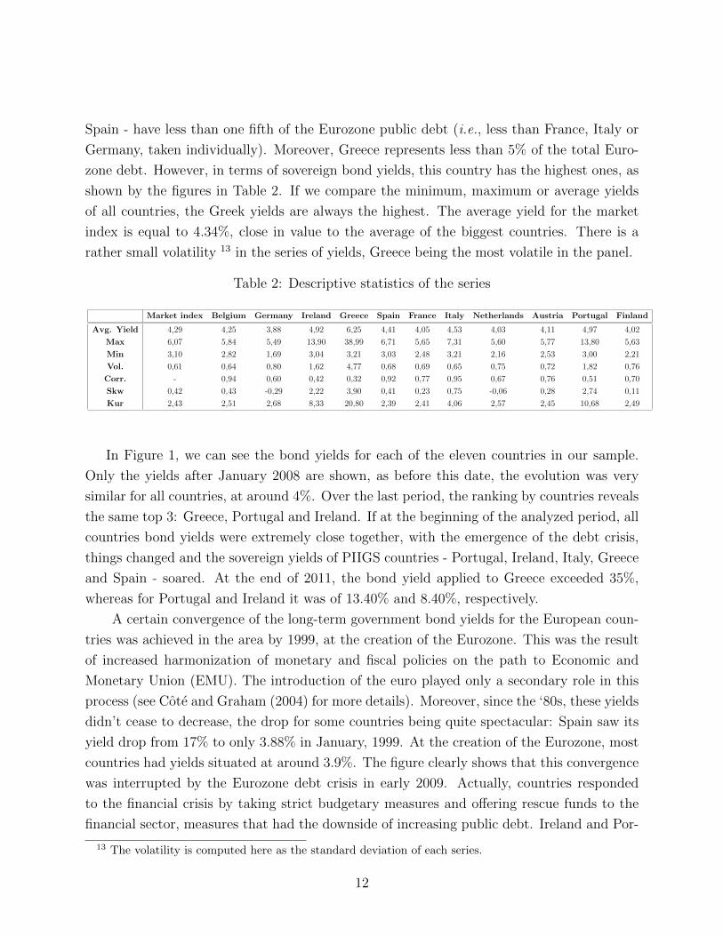
Spain - have less than one fifth of the Eurozone public debt (i.e., less than France, Italy or

Germany, taken individually). Moreover, Greece represents less than 5% of the total Euro-

zone debt. However, in terms of sovereign bond yields, this country has the highest ones, as

shown by the figures in Table 2. If we compare the minimum, maximum or average yields

of all countries, the Greek yields are always the highest. The average yield for the market

index is equal to 4.34%, close in value to the average of the biggest countries. There is a

rather small volatility 13 in the series of yields, Greece being the most volatile in the panel.

Table 2: Descriptive statistics of the series

Market index Belgium Germany Ireland Greece Spain France Italy Netherlands Austria Portugal Finland

Avg. Yield 4,29 4,25 3,88 4,92 6,25 4,41 4,05 4,53 4,03 4,11 4,97 4,02

Max 6,07 5,84 5,49 13,90 38,99 6,71 5,65 7,31 5,60 5,77 13,80 5,63

Min 3,10 2,82 1,69 3,04 3,21 3,03 2,48 3,21 2,16 2,53 3,00 2,21

Vol. 0,61 0,64 0,80 1,62 4,77 0,68 0,69 0,65 0,75 0,72 1,82 0,76

Corr. - 0,94 0,60 0,42 0,32 0,92 0,77 0,95 0,67 0,76 0,51 0,70

Skw 0,42 0,43 -0,29 2,22 3,90 0,41 0,23 0,75 -0,06 0,28 2,74 0,11

Kur 2,43 2,51 2,68 8,33 20,80 2,39 2,41 4,06 2,57 2,45 10,68 2,49

In Figure 1, we can see the bond yields for each of the eleven countries in our sample.

Only the yields after January 2008 are shown, as before this date, the evolution was very

similar for all countries, at around 4%. Over the last period, the ranking by countries reveals

the same top 3: Greece, Portugal and Ireland. If at the beginning of the analyzed period, all

countries bond yields were extremely close together, with the emergence of the debt crisis,

things changed and the sovereign yields of PIIGS countries - Portugal, Ireland, Italy, Greece

and Spain - soared. At the end of 2011, the bond yield applied to Greece exceeded 35%,

whereas for Portugal and Ireland it was of 13.40% and 8.40%, respectively.

A certain convergence of the long-term government bond yields for the European coun-

tries was achieved in the area by 1999, at the creation of the Eurozone. This was the result

of increased harmonization of monetary and fiscal policies on the path to Economic and

Monetary Union (EMU). The introduction of the euro played only a secondary role in this

process (see Cote and Graham (2004) for more details). Moreover, since the ‘80s, these yields

didn’t cease to decrease, the drop for some countries being quite spectacular: Spain saw its

yield drop from 17% to only 3.88% in January, 1999. At the creation of the Eurozone, most

countries had yields situated at around 3.9%. The figure clearly shows that this convergence

was interrupted by the Eurozone debt crisis in early 2009. Actually, countries responded

to the financial crisis by taking strict budgetary measures and offering rescue funds to the

financial sector, measures that had the downside of increasing public debt. Ireland and Por-

13 The volatility is computed here as the standard deviation of each series.

12

Figure 1: Bond yields by country

tugal are the countries that have experienced the largest increase in their debt during the

financial crisis, whereas Greece and Italy have had historically high levels of public debt.

And when investors lose confidence in a country’s ability to repay its debt, high levels of

debt are sanctioned by higher yields.

Figure 2: Government Bond Yield Index

13

Figure 2 provides the evolution of the index. The bond yield for the Eurozone,

constructed using countries’ bond yields and debt weights, is increasing since the second

half of 2010. At the end of the analyzed time span, its value is much higher than the ones

registered at any moment before. This is due to a sharp increase in the yields and captures

the present economic turmoil.

Figure 3: Debt Shortfall by country

In Figure 3, we can see that Italy is the country that, in stress periods, has the highest

Debt Shortfall, thus the highest need to get financed. This makes Italy a systemically

important country. Not surprisingly, Greece comes next, over the last period. Thus, even if

this country accounts for less than 5% of the Eurozone debt, the figure shows that Greece is

certainly systemically risky, with a sharp increase of its Debt Shortfall during 2011. Recall

that during this year, financial markets became increasingly worried about a possible exit

of Greece from the Eurozone, the Greek parliament voted drastic austerity measures and

the European Union (EU) agreed on helping the country with several billion euros. During

the same year, Greece was downgraded several times by credit rating agencies and reached

the lowest investment-grade rating. All these events contributed to the abrupt increase in

Greek yields. This graph reveals the importance of our measure: if we choose to analyze

14

the data based only on the primary deficit, we get a ranking that always places Germany

on the first position. Therefore, the riskiness of countries such as Italy and Greece will only

be partially captured.

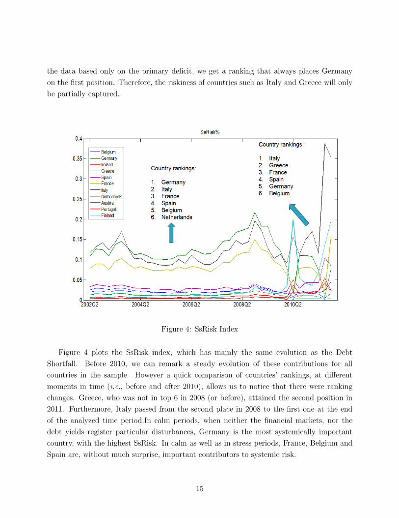
Figure 4: SsRisk Index

Figure 4 plots the SsRisk index, which has mainly the same evolution as the Debt

Shortfall. Before 2010, we can remark a steady evolution of these contributions for all

countries in the sample. However a quick comparison of countries’ rankings, at different

moments in time (i.e., before and after 2010), allows us to notice that there were ranking

changes. Greece, who was not in top 6 in 2008 (or before), attained the second position in

2011. Furthermore, Italy passed from the second place in 2008 to the first one at the end

of the analyzed time period.In calm periods, when neither the financial markets, nor the

debt yields register particular disturbances, Germany is the most systemically important

country, with the highest SsRisk. In calm as well as in stress periods, France, Belgium and

Spain are, without much surprise, important contributors to systemic risk.

15

Figure 5: SsRisk and Default probabilities as of 2011 Q4

Figure 5 plots the SsRisk measure against the probability of default of each country, that

is the probability of experiencing a systemic event. At the end of 2011, Greece and Italy

were the countries with the highest probabilities of default, but also with the most important

levels of SsRisk. For these countries, this underlines the danger of not only being con-

fronted with a default, but also needing an important amount of funds in order to be rescued.

By using the same type of graph, in Figure 6 we perform a comparison between the

situation before the crisis - first quarter of 2006 and after the emergence of the sovereign debt

turmoil - last quarter of 2011. If we compare stress and calm periods, we notice that in 2006,

countries are clustered together, having small needs of funding and low default probabilities.

However in 2011, the probability of default becomes higher for all the countries (compared

to 2006) and their SsRisk also gets more important, especially for countries as Italy or Greece.

When we analyze two countries in particular, for example, Greece and Germany, we can

easily see in figure 7 that there is a small increase in the probability of default and SsRisk in

Germany (at different moments in time) while in Greece, both the SsRisk and the probability

increased sharply between 2002 and 2011, making this country systemically risky.

16

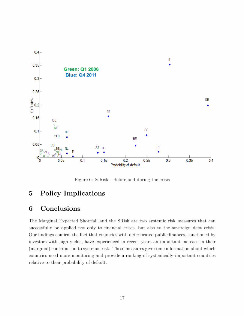
Figure 6: SsRisk - Before and during the crisis

5 Policy Implications

6 Conclusions

The Marginal Expected Shortfall and the SRisk are two systemic risk measures that can

successfully be applied not only to financial crises, but also to the sovereign debt crisis.

Our findings confirm the fact that countries with deteriorated public finances, sanctioned by

investors with high yields, have experienced in recent years an important increase in their

(marginal) contribution to systemic risk. These measures give some information about which

countries need more monitoring and provide a ranking of systemically important countries

relative to their probability of default.

17

(a)

(b)

Figure 7: A country comparison

References

[1] Acharya V., Pedersen L.H., Philippon T., Richardson M.P. (2010), “Measuring Systemic

Risk”, AFA 2011 Denver Meetings Paper

[2] Brownlees, C.T. and Engle, R. (2011), “Volatility, Correlation and Tails for Systemic

Risk Measurement”, Working Paper, NYU-Stern

18

[3] Scaillet, O. (2005), “Nonparametric estimation of conditional expected shortfall”, In-

surance and Risk Management Journal, vol.74, pp. 639-660.

[4] Silverman, B. W. (1986), “Density Estimation for Statistics and Data Analysis”, Chap-

man & Hall/CRC

[5] Simonoff, J. (1996) “Smoothing Methods in Statistics”, Springer Series in Statistics

[6] Wand, M. P. and Jones, M. C. (1995) “Kernel Smoothing”, London: Chapman and Hall

19

Appendix A: Details on the calculation of MES (1)

When computing the marginal expected shortfall, we make use of a detailed expression for

rit. As in the main text, the bond yield of country i and the yield of the market can be

written as Garch processes:

rit = σitεit

rmt = σmtεmt(25)

To unfold this expression, we use some standard results of the Capital Asset Pricing Model

(CAPM). Mainly, the yields for country i are such that:

rit = βirmt + µit, (26)

with µit an error term and βi estimated as in any linear regression:

βi =cov(ri, rm)

var(rm)=σimtσ2mt

. (27)

Moreover, the conditional correlation between the yield of country i and the market index

is given by:

ρimt =σimtσitσmt

, (28)

which allows us to rewrite the equation of rit as:

rit = σimtσ2mtσmtεmt + µit

= σimtσmt

εmt + µit

= σimtσmtσit

σitεmt + µit

= ρimtσitεmt + σµitξit,

(29)

where µit is the residual of the linear regression and ξit is the standardized residual. Fur-

thermore, knowing that εmt and ξit are orthogonal and standard normally distributed, the

variance of rit, σ2it = ρ2imtσ

2it + σ2

µit, gives us an expression for the variance of the residuals:

σ2µit = σ2

it(1− ρ2imt), (30)

20

and thus, their standard error:

σµit = σit

√(1− ρ2imt). (31)

Finally, putting all these results together, we obtain the formula for the returns of asset i we

are looking for:

rit = ρimtσitεmt + σit√

(1− ρ2imt)ξit= σit (ρimtεmt +

√(1− ρ2imt)ξit)︸ ︷︷ ︸εit

(32)

Appendix B: Details on the calculation of MES (2)

Departing from the expression for the expected shortfall of the Eurozone system at time t,

ESm,t−1(C) = Et−1(rmt|rmt > C). (33)

we follow Scaillet (2005) and show that the first order derivative with respect the the weight

associated with the ith country, i.e. MES, is given by

∂ESm,t−1(C)

∂wi= ET−1(rit|rm > C). (34)

For this, we denote by rmt the yield applied to the system except for the contribution

of the ith country, where rmt =∑n

j=1 j 6=iwjrjt and rmt = rmt + wirit. Besides, we do not

restrict the threshold C to be a scalar. It is assumed to depend on the distribution of the

market yield and hence on the weights and the specified probability to be in the tail of the

distribution p, as in the case of the V aR, thus providing a general proof for eq. 34.

It follows that

ESm,t−1(C) = Et−1(rmt + wirit|rmt + wirit > C(wi, p))

=1

p

∞∫−∞

∞∫C(wi,p)

(rmt + wirit)f(rmt, rit) drmt

drit,(35)

where f(rmt, rit) stands for the joint probability density function of the two series of yields.

21

Consequently,

∂ESm,t−1(C)

∂wi=

1

p

∞∫−∞

∞∫C(wi,p)

(rit)f(rmt, rit) drmt

drit

− 1

p

∞∫−∞

(∂C(wi, p)

∂wi− rit

)C(wi, p)f (C(wi, p)− wirit, rit) drit

(36)

However, the probability to be in the right tail of the distribution of the market yields is

constant, i.e. Pr (rmt + wirit > C) = p. A direct implication of this fact is that the first

order derivative of this probability is null. To put it differently, using simple calculus rules

for cumulative distribution functions, it can be shown that(∂C(wi, p)

∂wi− rit

)f (C(wi, p)− wirit, rit) = 0. (37)

Therefore, eq. 36 can be written compactly as

∂ESm,t−1(C)

∂wi=

1

p

∞∫−∞

∞∫C(wi,p)

(rit)f(rmt, rit) drmt

drit

= Et−1(rit|rmt + wirit > C(wi, p))

= Et−1(rit|rmt > C),

(38)

which completes the proof.

Appendix C: Tail Expectations

We show that the tail expectations Et−1(εmt|εmt > C/σmt) and Et−1(ξit|εmt > C/σmt) can

be easily estimated in a non-parametric kernel framework by elaborating on Scaillet (2005).

For ease of notation, let us note the systemic risk event C/σmt by κ. We first consider

the tail expectation on market yields Et−1(εmt|εmt > C/σmt), which becomes

Et−1(εmt|εmt > κ). (39)

Using the definition of the conditional mean, we rewrite 39 as a function of the probability

22

density function f

Et−1(εmt|εmt > κ) =

∞∫κ

εmtf(u|u > κ) du

=

∞∫−∞

εmtf(u|u > κ) du−κ∫

−∞

εmtf(u|u > κ) du,

(40)

where the conditional density f(u|u > κ) can be stated as

f(u)

Pr(u > κ). (41)

To complete the proof, we must compute the numerator and denominator in 41. For this,

we first consider the standard kernel density estimator of the density f at point u given by

f(u) =1

Th

T∑1

φ(u− εmt

h),

where h stands for the bandwidth parameter, and T is the sample size (Silverman, 1986,

Wand and Jones, 1995, Simonoff, 1996). Second, the probability to be in the tail of the

distribution can be defined as the integral of the probability density function over the domain

of definition of the variable u, i.e. p = Pr(u > κ) =∞∫κ

f(u) du. Consequently, by replacing

f(u) with the kernel estimator, we obtain

p =1

Th

T∑t=1

(1− Φ(

κ− εmth

)

).

The expectation in 39 takes hence the form

Et−1(εmt|εmt > κ) =

T∑t=1

εmt(1− Φ(κ−εmt

h))

T∑t=1

(1− Φ(κ−εmt

h)) . (42)

23

Similarly, it can be shown that

Et−1(ξit|εmt > κ) =

T∑t=1

ξit(1− Φ(κ−εmt

h))

T∑t=1

(1− Φ(κ−εmt

h)) . (43)

24