sovereign spreads and contagion risks in asia - imf. · pdf filea credit event––...

Sovereign Spreads and Contagion Risks in Asia

Carlos Caceres and D. Filiz Unsal

WP/11/134

© 2011 International Monetary Fund WP/11/134 IMF Working Paper Asia and Pacific Department

Sovereign Spreads and Contagion Risks in Asia 1

Prepared by Carlos Caceres and D. Filiz Unsal

Authorized for distribution by Roberto Cardarelli

June 2011

Abstract

This Working Paper should not be reported as representing the views of the IMF. The views expressed in this Working Paper are those of the author(s) and do not necessarily represent those of the IMF or IMF policy. Working Papers describe research in progress by the author(s) and are published to elicit comments and to further debate.

This paper explores how much of the movements in the sovereign spreads of Asian economies over the course of the global financial crisis has reflected shifts in (i) global risk aversion; (ii) country-specific risks, directly from worsening fundamentals, and indirectly from spillovers originating in other sovereigns and the uncertainty surrounding exchange rates. Earlier in the crisis, the increase in market-implied contagion led to higher Asian sovereign bond yield spreads over swaps. But, after the crisis, Asia’s sovereign spreads normalized, despite the debt crisis in the euro area, reflecting a fall in both exchange rate and spillover risks.

JEL Classification Numbers: E43, E44, G01, G10.

Keywords: Sovereign spreads; contagion; exchange rates; market price of risk; fiscal policy.

Authors’ E-mail Addresses: [email protected], [email protected]

1Without any implication, we would like to thank Alberto Behar, Roberto Cardarelli, Raphael Espinoza, Vincenzo Guzzo, Kenneth Kang, Miguel Segoviano, and participants at the APD seminar, for constructive comments and discussions. We would also like to thank Julia Guerreiro and Souvik Gupta for excellent research assistance. Any errors are solely the authors’ responsibility.

2

Contents Page

I. Introduction ...................................................................................................................................... 3

II. Data and Construction of the Main Variables ................................................................................. 5

A. Global Risk Aversion ................................................................................................................ 7 B. Contagion and the Spillover Coefficient (SC)........................................................................... 8 C. Exchange Rate Risk ................................................................................................................... 8

III. Estimation Methodology and Main Results ................................................................................. 12

A. The Estimation Model ............................................................................................................. 12 B. Estimation Results ................................................................................................................... 13

IV. Discussion .................................................................................................................................... 14

V. Conclusions .................................................................................................................................. 16

References .......................................................................................................................................... 24

Box 1. The Exchange Rate Risk Index (ERRI) ......................................................................................... 11

Figures 1. Asian Countries’ Sovereign Swap Spreads ...................................................................................... 6 2. Index of Global Risk Aversion (IGRA) ........................................................................................... 7 3. Exchange Rate Risk Index (ERRI) ................................................................................................ 10 4. Contributions to Distress Dependence: Systemic Outbreak vs. Sovereign Risk Phase ................. 16

Annex I............................................................................................................................................... 18

Annex II ............................................................................................................................................. 20

Annex III ............................................................................................................................................ 22

3

I. INTRODUCTION

Over the past couple of years, sovereign yields have globally exhibited an unprecedented degree of volatility. In the months following the collapse of Lehman Brothers, the spread between government bonds and the interest rate on a swap (of the same maturity and currency denomination) rose sharply across the board. This phenomenon was also present in Asia. Likewise, the credit default swap––the premium investors are willing to pay to insure a given government bond against a credit event–– increased exponentially over this period. For instance, the CDS spread on Japanese sovereign bonds moved from below 20bp in early September 2008 to around 120bp at the height of the crisis. In Korea and the Philippines, these spreads increased around 600bp over that same period, whilst at the same time, and more strikingly, sovereign CDS spreads in Indonesia rose over 1000bp. In many cases, this was accompanied by a sharp depreciation of the currency,2 an increased volatility in the exchange rate, or a substantial drain in foreign reserves.

Movements in government bond yields can have significant macroeconomic consequences. A rise in sovereign yields tends to be accompanied by a widespread increase in long-term interest rates in the rest of the economy, affecting both consumption and investment decisions. On the fiscal side, higher government bond yields imply higher debt-servicing costs and can significantly raise funding costs. This could also lead to an increase in rollover risk, as debt might have to be refinanced at unusually high cost or, in extreme cases, cannot be rolled over at all. A large increase in government funding costs can thus cause real economic losses, in addition to the purely financial effects of higher interest rates.

At the height of the financial crisis, several factors might have led to the developments observed in sovereign bond markets. First, global risk aversion increased, as investors sought higher compensation for risk. Deleveraging and balance sheet-constrained investors developed a systemically stronger preference for a few selected assets vis-à-vis riskier instruments. This behavior not only benefited a few sovereign securities as an asset class at the expense of corporate bonds and other ‘riskier’ assets, but also introduced a higher degree of differentiation among sovereigns.

This paper intends to analyze the extent to which the large fluctuations observed in Asian sovereign spreads during the crisis reflected changes in global risk aversion or the insurgence of country-specific risk, via worse fundamentals, increased exchange rate risk, or contagion from other countries.

The literature on the recent developments in sovereign spreads worldwide is relatively vast. For instance, Hartelius and others (2008) look at the influence of liquidity and fundamentals––as embedded in the 3-month Federal Funds future rates and in credit ratings, respectively––on sovereign spreads in various emerging economies. They found that both are important determinants of emerging market spreads. Bellas and others (2010) look into the determinants of sovereign spreads in emerging markets by separating these into macroeconomic fundamentals and financial

2 Japan and China, for instance, were clear exceptions to this. In fact, Japan saw its exchange rate appreciate, whilst China maintained its exchange rate fixed relative to the U.S. dollar over this period.

4 stress factors, and found that the first tend to prevail over the long run, whilst financial volatility is more important in the short run. Several studies look into the relationship between sovereign bond spreads and measures of macroeconomic and fiscal fundamentals (e.g., Baldacc, Guptam, and Mati, 2008; Kamin and von Kleist, 1999; and Min, 1998). The latter are found to have an impact on the level of sovereign spreads in the case of specific countries or regions, and over certain time horizons.

Explicitly modeling sovereign spreads on measures of global risk aversion, distress dependence and exchange rate risk, separately from country-specific fiscal fundamentals, is one of the key aspects of this analysis. Other research papers have attempted to include proxies for global risk aversion in the analysis of sovereign spreads. However, some of these measures tend to be oversimplistic and can be affected by a wide range of factors, thus not capturing the specific concept of global risk aversion. For instance, the spreads of U.S. corporate bonds over treasury bonds,3 which are likely to be affected by a large number of institution-specific or country-specific factors, cannot be considered an exclusive measure of global risk aversion. The main benefit of such proxies is that they are based on observable measures and are therefore readily available.

Other methods rely on extracting the (unobserved) “risk aversion” component from the actual (observed) sovereign spread series—in other words “filtering.”4 Although statistically viable, these measures depend on the adopted data sample, as global risk aversion is assumed to be proxied by the time-varying common factor of the analyzed series. Our measure of global risk aversion is based on the methodology developed in Espinoza and Segoviano (2011). This measure is completely independent of our data sample, and does not change according to which countries are being considered.

In order to differentiate between the effects of global risk aversion and inherent risk of contagion on sovereign spreads, Caceres, Guzzo, and Segoviano (2010) used an original measure of distress dependence––or a spillover coefficient. This is an important twist in the story as it permits the separation of the effects stemming from global liquidity conditions to those of country-specific credit risk coming from distress in other countries. This distress dependence among sovereigns might be due to several factors. For instance, trade linkages might play an important role in an environment of slowing global demand. Capital flow linkages represent another possibility. Financial institutions tend to engage in important cross-border activities, and can therefore be another channel of contagion. In fact, several of these sovereigns were required––almost simultaneously––to provide support to the banks and other systemic financial institutions operating

3 Used in Codogno, Favero, and Missale (2003) and Schuknecht, von Hagen, and Wolswijk (2010).

4 For example, Geyer, Kossmeier, and Pichler (2004) extract the common factor embedded in EMU spreads based on the use of a Kalman filter. Sgherri and Zoli (2009) apply a Bayesian filtering technique to extract the time-varying common factor from a nonlinear model of the sovereign spreads.

5 on their domestic markets. Finally, there could be contingent liabilities from one sovereign to another; these might be explicit or simply perceived by the market to be the case.5

By explicitly differentiating among distress dependence, global risk aversion, and country-specific fundamentals, Caceres, Guzzo and Segoviano (2010) identify the individual effects of each of these factors on sovereign spreads. However, their analysis centered on the study of sovereign spreads for the euro area. This is an important aspect to bear in mind, as euro area countries operate in a specific environment, with a shared currency and a single monetary authority.6 This is not the case in the Asian economies in our sample. These countries have their own currencies, and decide upon the monetary and exchange rate regime in place. In order to take this into account, we introduce an innovative measure of exchange rate risk in this analysis. By doing so, we are able to differentiate between the effects of global risk aversion, exchange rate risk, contagion, and country-specific fiscal fundamentals on sovereign spreads in a broad range of emerging and advanced Asian economies.

This paper is organized as follows. Section II introduces the dataset and focuses on the construction of the global risk aversion, distress dependence and exchange risk measures. Section III presents the estimation model and results, whereas Section IV assesses the main findings. Section V concludes.

II. DATA AND CONSTRUCTION OF THE MAIN VARIABLES

We measure spreads in Asian countries as the spreads of sovereign bond yields to the swap rate (fixed rate leg of interest rate swap) of the same maturity and same currency denomination as the bond. In other words, this is the yield at which one party is willing to pay a fixed rate in order to receive a floating rate from a given counterparty. Typically, the yield on an AAA-rated government bond––such as those of Australia and New Zealand–– would trade below the swap yield. In contrast, yields on lower-rated bonds might be above the swap yield as investors demand a higher premium on these riskier assets.

The resulting dataset spans from the beginning of 2005, well ahead of the start of the crisis, through mid 2010, encompassing eleven Asian sovereign markets.7 The paths of these spreads since mid-2007 are shown in Figure 1. In the period before September 2008, most of these spreads remained within a relatively narrow, albeit widening, range. In some cases (e.g., Hong Kong), sovereign bond yields held or fell further below the swap yield as bank counterparty risk was weighing adversely on swaps. Following this period of ‘financial crisis build-up’, three phases can

5 For instance, market agents might believe that one or more countries would come to the rescue of other countries if the latter were to fall in distress. A country in distress is effectively considered as a contingent liability for the other countries.

6 In principle, unlike banks, sovereigns could prevent excessive funding pressures if they borrowed in their own currency and had a floating exchange rate. This is not the case in euro area countries which borrow in a currency that they cannot directly control.

7 The sample is made of three advanced economies (Australia, Japan, and New Zealand), and six emerging market economies (China, Hong Kong, India, Indonesia, Korea, Malaysia, the Philippines, and Thailand).

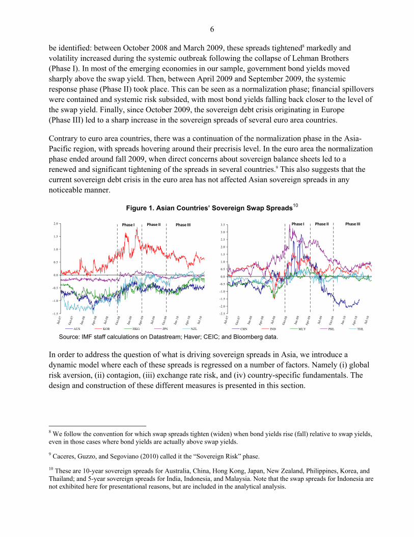
6 be identified: between October 2008 and March 2009, these spreads tightened8 markedly and volatility increased during the systemic outbreak following the collapse of Lehman Brothers (Phase I). In most of the emerging economies in our sample, government bond yields moved sharply above the swap yield. Then, between April 2009 and September 2009, the systemic response phase (Phase II) took place. This can be seen as a normalization phase; financial spillovers were contained and systemic risk subsided, with most bond yields falling back closer to the level of the swap yield. Finally, since October 2009, the sovereign debt crisis originating in Europe (Phase III) led to a sharp increase in the sovereign spreads of several euro area countries.

Contrary to euro area countries, there was a continuation of the normalization phase in the Asia-Pacific region, with spreads hovering around their precrisis level. In the euro area the normalization phase ended around fall 2009, when direct concerns about sovereign balance sheets led to a renewed and significant tightening of the spreads in several countries.9 This also suggests that the current sovereign debt crisis in the euro area has not affected Asian sovereign spreads in any noticeable manner.

Figure 1. Asian Countries’ Sovereign Swap Spreads10

Source: IMF staff calculations on Datastream; Haver; CEIC; and Bloomberg data.

In order to address the question of what is driving sovereign spreads in Asia, we introduce a dynamic model where each of these spreads is regressed on a number of factors. Namely (i) global risk aversion, (ii) contagion, (iii) exchange rate risk, and (iv) country-specific fundamentals. The design and construction of these different measures is presented in this section.

8 We follow the convention for which swap spreads tighten (widen) when bond yields rise (fall) relative to swap yields, even in those cases where bond yields are actually above swap yields.

9 Caceres, Guzzo, and Segoviano (2010) called it the “Sovereign Risk” phase.

10 These are 10-year sovereign spreads for Australia, China, Hong Kong, Japan, New Zealand, Philippines, Korea, and Thailand; and 5-year sovereign spreads for India, Indonesia, and Malaysia. Note that the swap spreads for Indonesia are not exhibited here for presentational reasons, but are included in the analytical analysis.

-1.5

-1.0

-0.5

0.0

0.5

1.0

1.5

2.0

AUS KOR HKG JPN NZL

Phase I Phase II Phase III

-2.5

-2.0

-1.5

-1.0

-0.5

0.0

0.5

1.0

1.5

2.0

2.5

3.0

3.5

CHN IND MLY PHL THL

Phase I Phase II Phase III

7

A. Global Risk Aversion

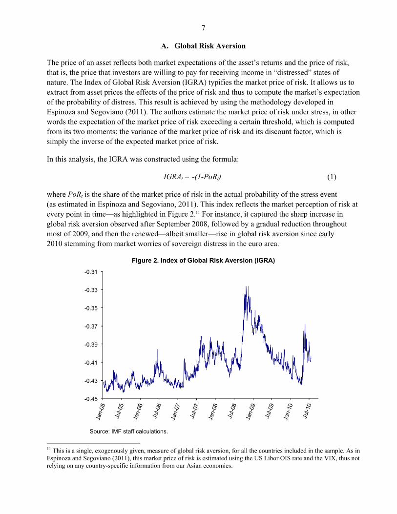
The price of an asset reflects both market expectations of the asset’s returns and the price of risk, that is, the price that investors are willing to pay for receiving income in “distressed” states of nature. The Index of Global Risk Aversion (IGRA) typifies the market price of risk. It allows us to extract from asset prices the effects of the price of risk and thus to compute the market’s expectation of the probability of distress. This result is achieved by using the methodology developed in Espinoza and Segoviano (2011). The authors estimate the market price of risk under stress, in other words the expectation of the market price of risk exceeding a certain threshold, which is computed from its two moments: the variance of the market price of risk and its discount factor, which is simply the inverse of the expected market price of risk.

In this analysis, the IGRA was constructed using the formula:

IGRAt = -(1-PoRt) (1)

where PoRt is the share of the market price of risk in the actual probability of the stress event (as estimated in Espinoza and Segoviano, 2011). This index reflects the market perception of risk at every point in time––as highlighted in Figure 2.11 For instance, it captured the sharp increase in global risk aversion observed after September 2008, followed by a gradual reduction throughout most of 2009, and then the renewed––albeit smaller––rise in global risk aversion since early 2010 stemming from market worries of sovereign distress in the euro area.

Figure 2. Index of Global Risk Aversion (IGRA)

Source: IMF staff calculations.

11 This is a single, exogenously given, measure of global risk aversion, for all the countries included in the sample. As in Espinoza and Segoviano (2011), this market price of risk is estimated using the US Libor OIS rate and the VIX, thus not relying on any country-specific information from our Asian economies.

-0.45

-0.43

-0.41

-0.39

-0.37

-0.35

-0.33

-0.31

8

B. Contagion and the Spillover Coefficient (SC)

Contagion is captured by a measure of distress dependence––the Spillover Coefficient (SC)—which characterizes the probability of distress of a country conditional on other countries (in the sample) becoming distressed. This indicator embeds distress dependence across sovereign credit default swaps (CDS) and their changes throughout the economic cycle, reflecting the fact that dependence increases in periods of distress. The SC is based on the methodology presented in Segoviano and Goodhart (2009)12 and is computed in four steps:

(i) The marginal probabilities of default for countries Ai and Aj, P(Ai) and P(Aj) respectively, are extracted from the individual CDS spreads for these countries.13

(ii) Then, the joint probability of default of Ai and Aj, P(Ai, Aj), is obtained using the CIMDO methodology developed by Segoviano (2006). This methodology is used to estimate the multivariate empirical distribution (CIMDO-distribution) that characterizes the probabilities of distress of each of the sovereigns under analysis, their distress dependence, and how such dependence changes along the economic cycle. The CIMDO methodology is a nonparametric methodology, based on the Kullback (1959) cross-entropy approach, which does not impose parametric predetermined distributional forms, whilst being constrained to characterize the empirical probabilities of distress observed for each institution under analysis (extracted from the CDS spreads). The joint probability of distress of the entire group of sovereigns under analysis and all the pair wise combinations of sovereigns within this group, that is, P(Ai, Aj), are estimated from the CIMDO-distribution.

(iii) The probability of sovereign distress in country Ai given a default by country Aj, expressed as the conditional probability of default P(Ai/Aj), is obtained using the Bayes’ law: P(Ai/Aj) = P(Ai,Aj) / P(Aj).

(iv) Finally, for each country Ai, the SC is computed using the formula:

SC(Ai) = ∑ P(Ai/Aj) · P(Aj) for all j ≠ i (2)

which is essentially the weighted sum of the probability of distress of country Ai given a default in each of the other countries in the sample. This measure of distress dependence is appropriately weighed by the probability of each of these events to occur.

C. Exchange Rate Risk

Exchange rates have exhibited a significant degree of volatility in recent years. In particular, at the height of the financial crisis, flight to safety led to a sharp appreciation of currencies deemed as safe

12 The SC was introduced in Caceres, Guzzo, and Segoviano (2010) which used this measure to characterize distress dependence among euro area countries.

13 We assume a recovery rate of 40 percent for sovereigns, as commonly used in the literature. However, since the SC is a relative, unit-less measure, the results are unchanged if the latter is scaled by a constant factor.

9 havens14, accompanied by the corresponding depreciation in several (less liquid) currencies. Similarly, the financial crisis led to a reversal in currency carry trades, implying a sharp depreciation in currencies that had previously experienced long appreciation sprints. These sharp movements in exchange rates might have significant effects on market expectations about future developments in the currency spectrum, in turn affecting demand for bonds denominated in a particular currency. In addition, exchange rate movements can have an important impact on sovereign risk perceptions if, for instance, most of the public debt of a given country is in a foreign denomination. More indirectly, sovereign risk might also increase due to implicit guarantees stemming from private sector holdings of sizeable liabilities denominated in foreign currency.

In order to assess the potential impact of exchange rate developments on sovereign spreads, we construct a measure of exchange rate risk––the Exchange Rate Risk Index (ERRI). The ERRI not only takes into account changes in the level of the exchange rate, but it also includes a measure of the volatility in the exchange rate. As suggested above, increased volatility––and thus uncertainty––in the currency market could play an important role in the perceived valuation of sovereign risk.

Some countries in our sample have a fixed exchange rate. This does not mean that the actual or perceived exchange risk is zero. Indeed, several countries in the world experienced large exchange rate pressures at the height of the financial crisis, which translated into significant changes in the amount of foreign reserves held by these countries. In acute cases, there could be a substantial risk that a country runs out of reserves, forcing it to abandon the peg and depreciating the currency. In order to capture these dynamics, the ERRI also includes a measure of exchange risk associated with changes in foreign reserve holdings.

Overall, the ERRI was constructed as a single indicator of exchange risk, which includes measures of recent currency depreciations (or appreciations), exchange rate volatility, and changes in foreign reserves. The index was compiled using Principal Component Analysis (PCA), using data for the 11 Asian economies in our sample––see Box 1 for details. Figure 3 exhibits the ERRI for our countries’ sample since the beginning of 2007. A fall in the index is perceived as an increase in the exchange rate associated risk, which could be due to a sharp depreciation,15 an increase in volatility, a fall in foreign reserves, or a combination of these.

Note that the ERRI captures well the sharp depreciation of currencies such as the Korean Won (KRW), the Australian Dollar (AUD) and the New Zealand Dollar (NZD) at the height of the financial crisis, the last two partially reflecting a reversal of the carry-trade against the Japanese Yen (JPY), accompanied by a significant appreciation of the latter, also captured by the ERRI. In fact, these four currencies, together with the Indonesian rupiah (IDR), experienced a significant increase in the volatility of their exchange rate at the time, also contributing to a lower value of the ERRI for those currencies. Finally, countries such as Malaysia, Korea, and Indonesia witnessed an important fall (in percentage points) in foreign reserves, which had, again, a negative contribution

14 The Japanese Yen (JPY) is an example of such currencies within our sample.

15 In this analysis, we considered the U.S. Dollar (USD) to be the common numeraire. Thus depreciation here indicates a depreciation of a given currency against the USD.

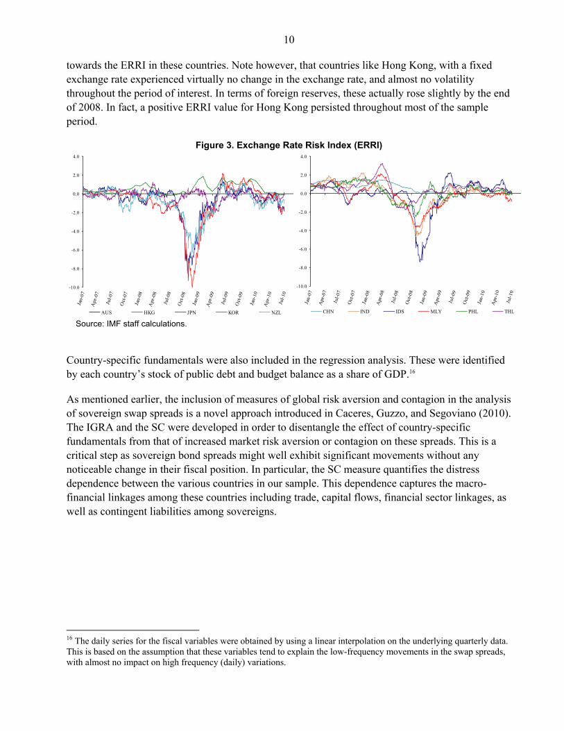
10 towards the ERRI in these countries. Note however, that countries like Hong Kong, with a fixed exchange rate experienced virtually no change in the exchange rate, and almost no volatility throughout the period of interest. In terms of foreign reserves, these actually rose slightly by the end of 2008. In fact, a positive ERRI value for Hong Kong persisted throughout most of the sample period.

Figure 3. Exchange Rate Risk Index (ERRI)


Country-specific fundamentals were also included in the regression analysis. These were identified by each country’s stock of public debt and budget balance as a share of GDP.16

As mentioned earlier, the inclusion of measures of global risk aversion and contagion in the analysis of sovereign swap spreads is a novel approach introduced in Caceres, Guzzo, and Segoviano (2010). The IGRA and the SC were developed in order to disentangle the effect of country-specific fundamentals from that of increased market risk aversion or contagion on these spreads. This is a critical step as sovereign bond spreads might well exhibit significant movements without any noticeable change in their fiscal position. In particular, the SC measure quantifies the distress dependence between the various countries in our sample. This dependence captures the macro-financial linkages among these countries including trade, capital flows, financial sector linkages, as well as contingent liabilities among sovereigns.

16 The daily series for the fiscal variables were obtained by using a linear interpolation on the underlying quarterly data. This is based on the assumption that these variables tend to explain the low-frequency movements in the swap spreads, with almost no impact on high frequency (daily) variations.

-10.0

-8.0

-6.0

-4.0

-2.0

0.0

2.0

4.0

AUS HKG JPN KOR NZL

-10.0

-8.0

-6.0

-4.0

-2.0

0.0

2.0

4.0

CHN IND IDS MLY PHL THL

11

Box 1. The Exchange Rate Risk Index (ERRI)

In several countries, exchange rate related risks seem to have played an important part in explaining the movements in sovereign spreads during the recent global financial crisis. There are various mechanisms through which exchange rate related developments might affect expectations about sovereign risk. In particular, a sharp depreciation of the exchange rate might lead to concerns about significant valuation changes in the stock of public debt of a country, especially if a sizable share of this debt is denominated in a foreign currency. Other more indirect mechanisms such as worries about contingent liabilities emanating from a highly geared private sector whose liabilities (or part of these) are in a foreign currency denomination might also be part of the story. Similarly, increased volatility in exchange markets is accompanied by a rise in uncertainty, which might lead to the tightening of sovereign spreads in some countries––in some cases due to, for example, flight to quality. Finally, even in a fixed exchange rate setting, currency risks still exist. In particular, a country might run out of foreign reserves whilst attempting to maintain a peg. These changes in reserves might be seen as another source of currency or exchange rate risk. We tried to capture the above notions related to currency risk in a single indicator: the Exchange Rate Risk Index (ERRI). Basically, the ERRI includes (i) a measure of currency depreciation (or appreciation), (ii) a measure of exchange rate volatility, and (iii) a measure reflecting changes in foreign reserves. For the measure of currency depreciation (or appreciation), we considered at each point in time the percentage change in the exchange rate (against the U.S. dollar) relative to its level 3-months earlier (roughly 65 days earlier using working days series). For the measure of volatility, we considered the same exchange rate daily series, and we computed the 3-month rolling averages of the absolute deviation between the log-value of the exchange rate on

a given day and the log-value of the exchange rate the day before, that is: ∑ | |, where

EXRt denotes the exchange rate level at time t, and T is 65 working days. Finally, the measure of foreign reserves changes was simply computed as the percentage change in foreign reserves at a given date relative to three months earlier.17 The ERRI was then computed by aggregating these three measures into a single index. First, we considered the z-score transformation for each of these three measures across all countries in our sample and across the entire period under consideration (from January 1, 2005 to June 30, 2010). Then, in order to estimate the relative weights of each of these three variables in the ERRI, we used Principal Component Analysis (PCA). The procedure of PCA consists of searching the linear combination(s) of the variables which produces the highest possible variance in the available data. This combination is the first (principal) component. More precisely, the principal component is extracted as the eigenvector associated with the largest eigenvalue of the correlation matrix of the underlying variables. In theory, there can be as many (principal) components as the total number of variables. However, the practical idea behind PCA is to have one or a few components explaining a large portion of the total variance in the data. This is what renders the interpretation of the results relatively easy in any practical application.18 The ERRI was thus obtained as the principal component of the above three standardized variables with coefficients: 0.63 for an appreciation in the exchange rate, -0.49 for an increase in volatility, and 0.61 for an increase in foreign reserves. –––––––––––––– 1/ Note that the foreign reserve series used were available at a monthly frequency only. Thus, the daily series of changes in foreign reserves were obtained by linearly interpolating the monthly series. In addition, we also tried variants of the ERRI using 6-month and 12-month changes in exchange rate, volatility and reserves, but these yielded essentially the same results as those using 3-month changes presented here.

2/ See Jollifee (2002) for a detailed discussion on the PCA methodology, and Behar (2009) and Caceres and Piperno Beer (2009) for practical applications of this methodology.

12 Contrary to simple correlations, or relationships based on the first few moments of different default probability series, the CIMDO methodology enables us to characterize the entire distributional links between these series, that is, linear (correlations) and nonlinear distress dependence, and their evolution throughout the economic cycle. This reflects the fact that dependence increases in periods of distress. Such dependence structure is characterized by a copula function (CIMDO-copula), which changes at each period in time, consistently with changes in the empirically observed distress probabilities.17 This is a key technical improvement over traditional risk models, which usually account only for linear dependence (correlations) that are assumed to remain constant over the cycle, over a fixed period of time, or over a rolling window of time.

Finally, this study extends the analysis of sovereign spreads presented in Caceres, Guzzo, and Segoviano (2010) by including a measure of exchange rate risk. The ERRI is an important contribution when analyzing the behavior of sovereign spreads in different countries not using the same currency or not pertaining to a given monetary union. This will be shown here to be a fairly important factor in explaining sovereign spread in most of the Asian countries included in our sample.

III. ESTIMATION METHODOLOGY AND MAIN RESULTS

A. The Estimation Model

The model used in the analysis of the determinants of sovereign swap spreads is described by the following General Autoregressive Conditional Heteroskedasticity (GARCH(1,1)) specification:

Yt = α Yt-1 + β’Xt + εt (3)

σt2 = ω + θ εt-1

2 + γ σt-12 (4)

where [3] is the mean equation for the swap spread Yt as a function of the explanatory variables stacked in the vector Xt (including a constant term), and an error term εt, with conditional variance σt

2. This conditional variance is given by equation [4] as function of the lag of the squared residual from the mean equation εt-1

2 (the ARCH term), and last period’s variance σt-12 (the GARCH term).

The explanatory variables include the Index of Global Risk Aversion (IGRA), a measure of distress dependence captured by the Spillover Coefficient (SC), our Exchange Rate Risk Index (ERRI), and two country-specific fiscal variables, namely the overall balance in percent of GDP and the debt-to-GDP ratio. The lag dependent variable is included in the model to capture the high persistence inherent in the daily time series of the swap spreads.18

The inclusion of measures of risk aversion, distress dependence and exchange rate risk––the IGRA, the SC and the ERRI, respectively - in the regression analysis of the sovereign swap spreads

17 See Segoviano and Goodhart (2009) for details.

18 The presence of the lag dependent variable mitigates the autocorrelation that would otherwise be observed in the residuals from estimating equation (3) without the lag dependent variable.

13 represents an original approach. This not only enables us to quantify the effect of these important factors on the dynamics of swap spreads, but it also mitigates the bias in the estimation of the coefficients for the country-specific fundamental variables that would otherwise arise from the omission of these three measures in the regression.19

B. Estimation Results

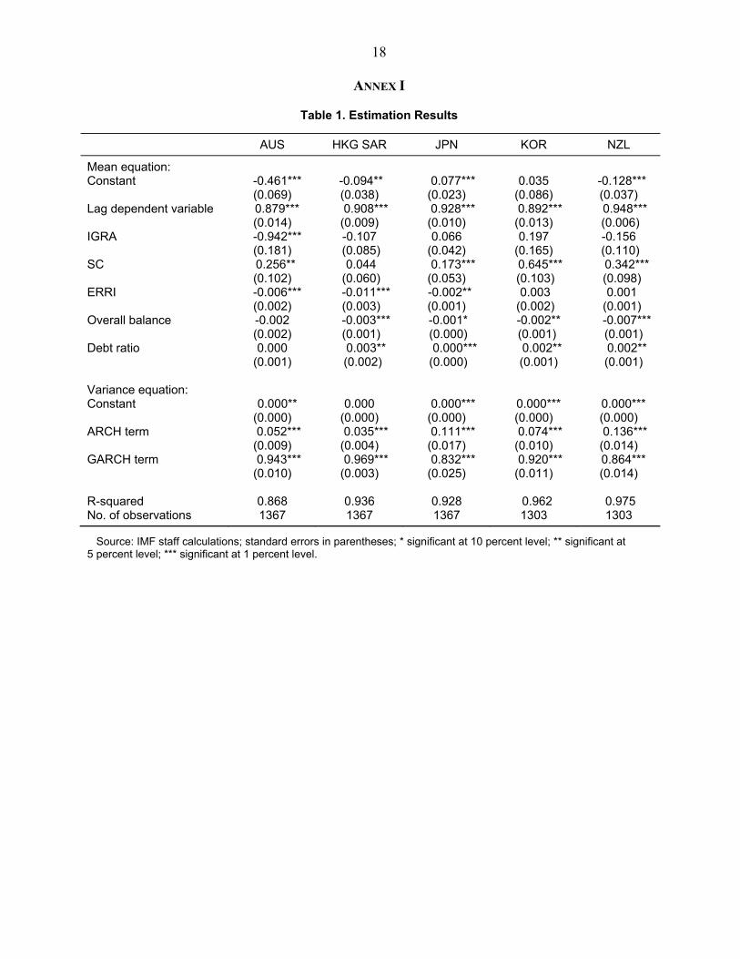
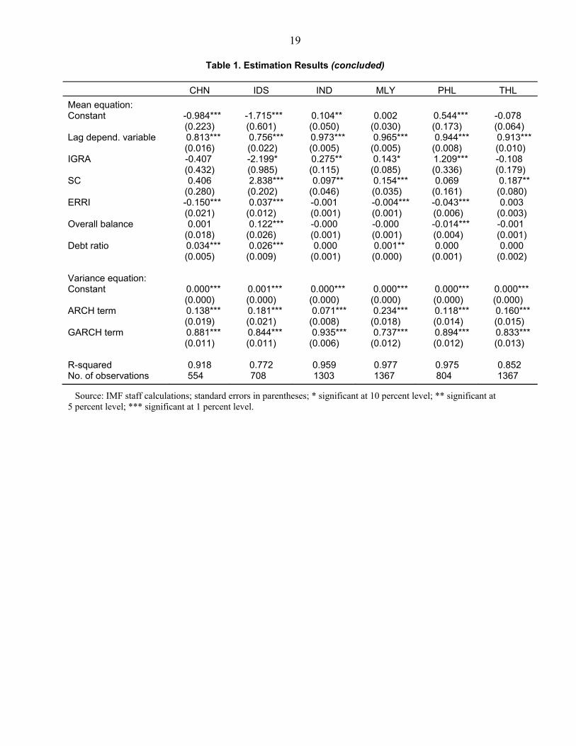
The results from the estimation of the model described by equations (3) and (4) are presented in Table 1 (see Annex I).20 The main findings can be summarized as follows:

(i) Contagion is always found to be negative for government bonds. When the probability of a credit event in a country (given distress in another sovereign issuer) rises, swap spreads tighten, as sovereign bond yields rise closer to the swap yield or move above that level. This relationship is significant for the vast majority of countries in our sample; in China, Hong Kong, and the Philippines, although with the expected sign, this relationship is not statistically significant. In contrast, we find that contagion has the strongest effect on sovereign spreads in Indonesia, followed by Korea and New Zealand.

(ii) Global risk aversion, in contrast, has very different effects on sovereign spreads among the countries in our sample. On the one hand, countries like Australia benefit from a generalized increase in risk aversion as investors switched to higher quality assets––or assets perceived as ‘safe heavens.’ On the other hand, countries such as the Philippines, India and Malaysia see their sovereign bond yields rising relative to the swap yield when global risk aversion rises.

(iii) Currency risk seems to be an important factor in explaining the behavior of sovereign spreads in Asia. Indeed, we found that a deterioration in our index exchange rate risk (ERRI) leads to a tightening of the swap spreads in most countries; the only exception being Indonesia. In particular, the sharp depreciations and increase in exchange rate volatility observed in the months following the collapse of Lehman Brothers explain an important share of the increase in bond yields relative to their respective swap rates.

(iv) Fiscal fundamentals also exhibit a significant relationship with these spreads. In general, swap spreads tighten, in other words sovereign bond yields rise versus swap yields when public debt ratios rise or budget balances deteriorate. Although relatively small, this effect seems to prevail in most of the advanced Asian economies,21 whilst the relationship is statistically weaker for the emerging countries in our sample.

19 A regression analysis that omits the effect of increased risk aversion, currency risk, or contagion might lead to an overestimation of the effects played by country-specific fundamentals.

20 The estimation of this model for all the countries in the sample was carried out in eViews via Maximum Likelihood Estimation, using the Marquardt Optimization Algorithm.

21 This is in line with the finding in Caceres, Guzzo, and Segoviano (2010) which find a statistically significant impact of fiscal fundamentals on sovereign spreads in ten euro area countries and two other (non-eurozone) EU members.

14

IV. DISCUSSION

On the back of this analysis, not only can we assess the sign and significance of the various factors on sovereign swap spreads––namely, global risk aversion, contagion, exchange rate risk, and country-specific fiscal fundamentals––but we can identify their contribution to the cumulative changes in spreads over the different periods of interest identified earlier on.

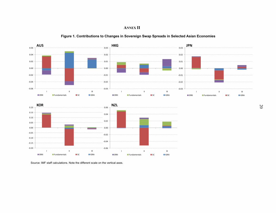
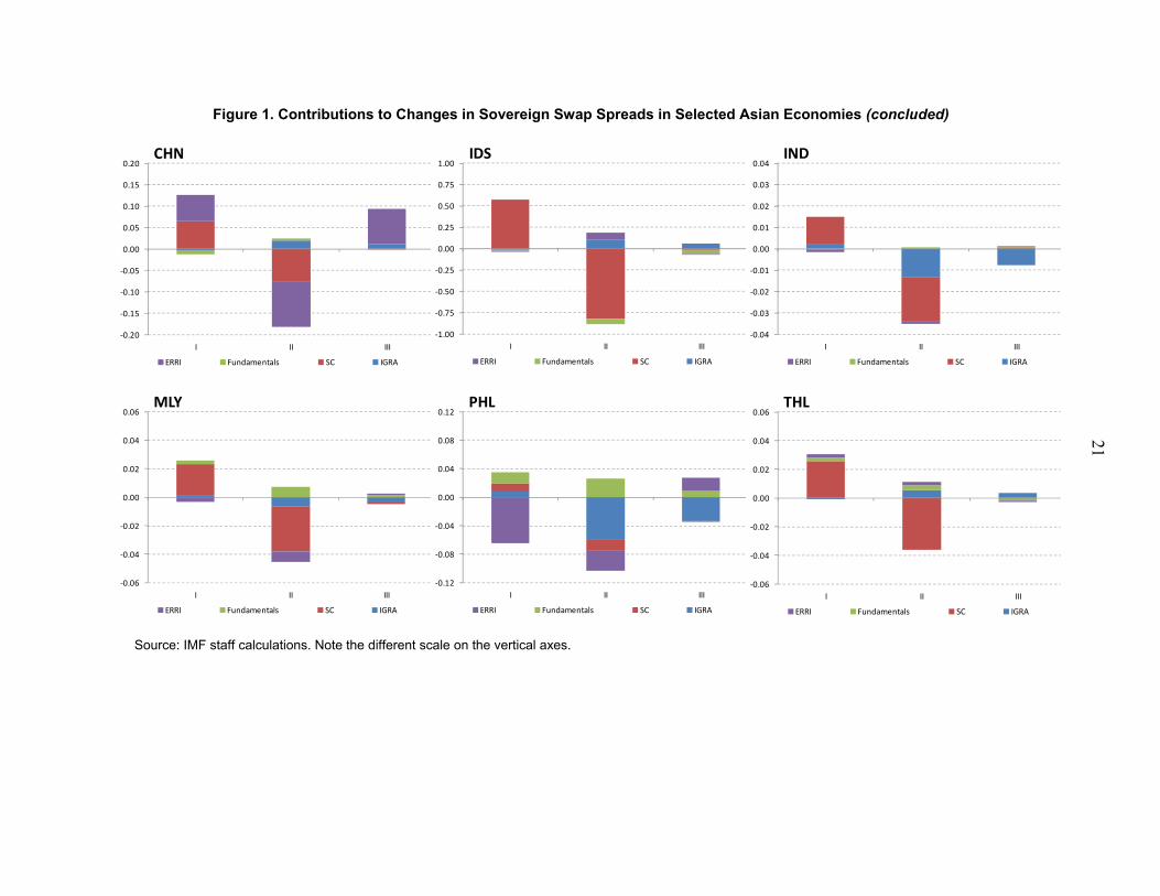
(i) During the systemic outbreak, between October 2008 and March 2009, all sovereign spreads in the Asian economies in our sample tightened (i.e., government bond yields rose relative to the swap) markedly. At the same time, global risk aversion rose sharply as financial sector strains propagated worldwide, accompanied by sharp rises in interbank and overnight spreads across the board. This increase in global risk aversion benefited a few government bonds––such as those of Australia, Hong Kong, and New Zealand––as investors’ moved to high-rated bonds, but only slightly as spreads in those countries still tightened noticeably overall. Indeed, the largest contributor to the rise in bond yields relative to swap yields was contagion among different sovereigns (see Annex II, Figure 4).

Despite the sharp depreciation observed in several of the countries in our sample and worsening fiscal fundamentals due to the slowdown in economic activity, these two factors only represented a relatively small share of the total contribution to the increase in bond yields relative to swap yields. In fact, in some countries––such as Hong Kong, where the peg to the dollar was maintained throughout this period, and was even accompanied by an increase in foreign reserve holdings––our measure of exchange rate-related risk played favorably for sovereign spreads (i.e., spreads widened).

(ii) During the systemic response phase, between April and September 2009, swap spreads widened (i.e., government bond yields fell back towards the swaps) across the board, as lower probabilities of distress in some countries were favorably affecting others. Indeed, most of the countries in our sample saw a reversal of the increase in bond yields relative to the swap due to contagion over the previous phase. On the negative side, fundamentals were still weak during this period, as the economic slowdown was well underway. However, these headwinds were not strong enough to outweigh the positive contribution from the fall in spillover risks among sovereigns.

The reduction in global risk aversion stopped benefitting the higher rated advanced economies in the region during this second phase. Instead, the increase in risk appetite benefited countries such as the Philippines, India and Malaysia. Furthermore, the fall in global risk aversion led to a depreciation of the dollar against several currencies worldwide, which implied a reduction in the perception of currency related risk in many of the advanced and emerging Asian economies.

(iii) Finally, in the sovereign risk phase, after October 2009, most sovereign spreads remained broadly unchanged throughout this period. In the few countries where sovereign spreads did tighten (e.g., Hong Kong and New Zealand), the increase in bond yields relative to swap yields was relatively small compared to the fall observed during the previous phase. In other words, this period can still be seen as an overall normalization phase for sovereign spreads in Asia, following the large shock observed during the systemic outbreak phase.

15 In addition, and contrary to many European countries, country-specific fundamentals have not played such an important role in the developments of sovereign spreads in Asia during the latter phase. In fact, in countries such as Hong Kong, fiscal balances started to improve again and the debt ratio was solidly on a downward trend and at low levels, thus contributing to a widening of the spreads.

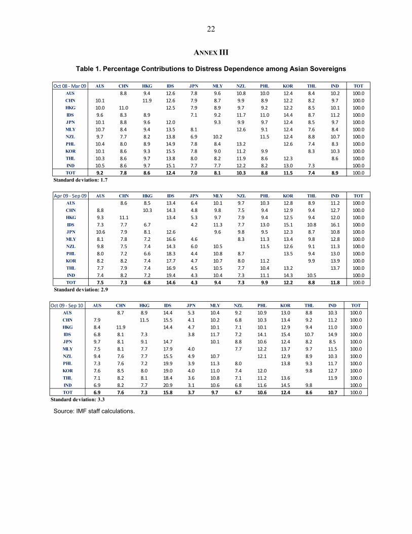
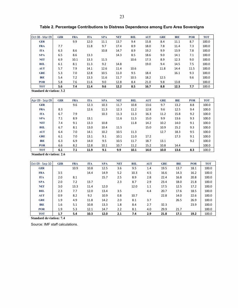
These observations differ substantially from the developments seen in the euro area during the sovereign risk phase. Caceres, Guzzo, and Segoviano (2010) noted that in countries such as Greece and Portugal, bond yields surged well above swap yields over that period as fundamentals weakened and the risks of contagion intensified. Those authors noted that contagion could be further broken down across sources of distress. In other words, for a given change in distress dependence of a specific sovereign, one can assess which countries are the largest contributors to sovereign spillovers during the three phases previously identified.22 The percentage contribution to the changes in each country’s SC––our measure of distress dependence––can be read along the rows of Tables 1 for Asian countries and Table 2 for the euro area (see Annex III).23

Once again, the story in Asian economies seems to differ markedly from that of euro area countries when it comes to the source of spillover risks among sovereigns. During the systemic outbreak, contagion gained significance in the euro area, and the countries having the largest contribution to the changes in SC were exactly those hit hard by the crisis, in particular, the small open economies with sizable financial sectors relative to the economy (e.g., Austria, Ireland, and the Netherlands). In Asia, the picture is a bit more blurry. First, there was not a significant difference between emerging and advanced countries regarding their contribution to changes in other countries’ SC. Indonesia and Korea presented the largest contribution during this period, whilst Japan followed by Thailand had the smallest share. Second, the dispersion between the relative contributions to the changes in SC from each of the countries in Asia was narrower than that of euro area countries during the systemic outbreak phase.24 In other words, it is more difficult in the case of Asia to attribute the bulk of the changes in SC to a specific country or a small group of countries (Figure 3).

In the recent sovereign risk phase, the emphasis shifted towards short-term financing risk and long-term sustainability of sovereign balance sheets. In the euro area, the countries putting pressure on other countries’ swap spreads were mainly Greece, Ireland, and Portugal. These three countries were responsible for over 58 percent of the contribution to changes in euro area’s SC over the year ending in September 2010. In our Asian sample, the contribution from the three largest contributors to the changes in SC over the same period represents less than 39 percent of the total (Tables 1

22 While conditional probabilities do not necessarily imply causation, they can provide important insights into interlinkages and the likelihood of contagion.

23 The last row in each table shows the (weighted)-average contribution to the changes in our distress dependence measure (SC) from each of the column countries. This is a proxy for the source of market-based contagion to the other countries in the sample, emanating from each of these countries over a particular period.

24 For instance, Austria contributed almost three times as much as Germany to changes in euro area SC. In the case of Asia, Indonesia (with the highest contribution) contributed 1.7 times as much as Japan (with the lowest contribution) to the changes in SC for the Asian sample.

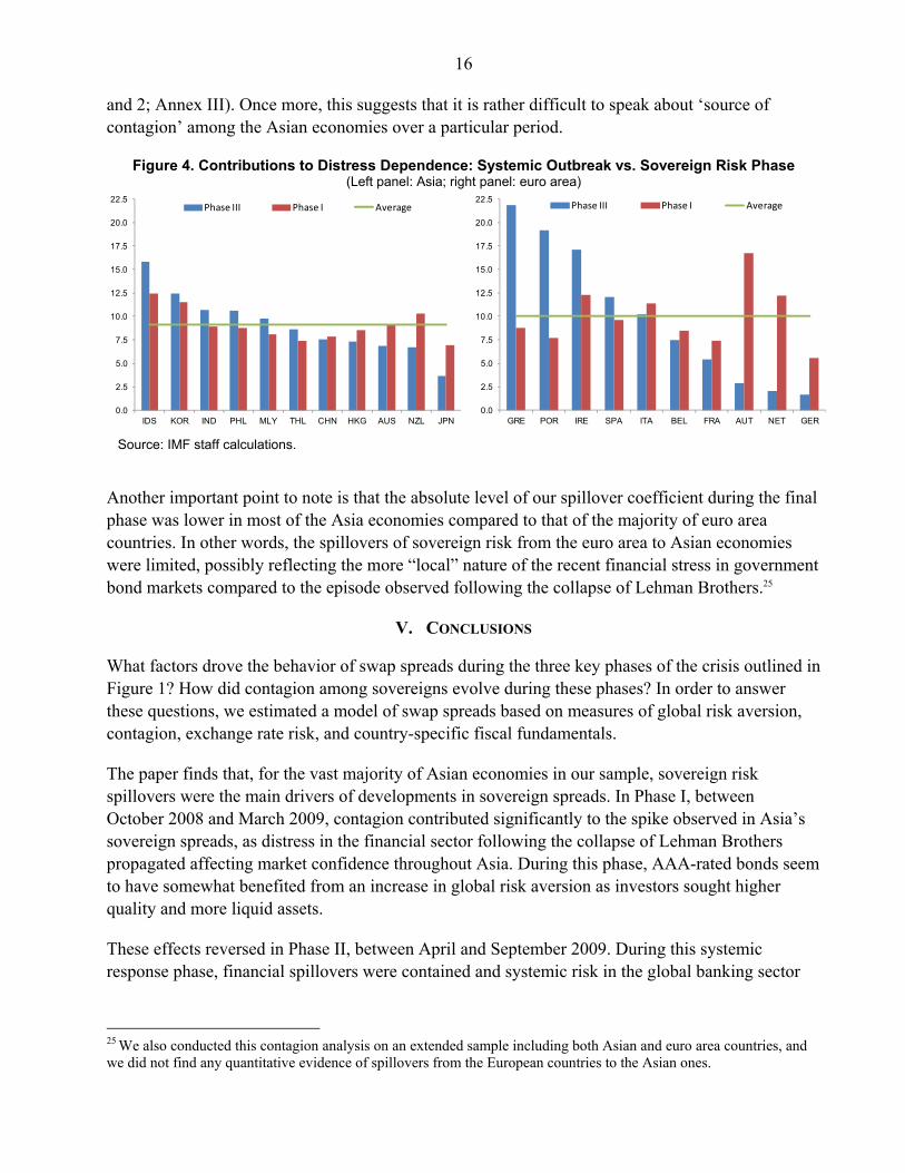
16 and 2; Annex III). Once more, this suggests that it is rather difficult to speak about ‘source of contagion’ among the Asian economies over a particular period.

Figure 4. Contributions to Distress Dependence: Systemic Outbreak vs. Sovereign Risk Phase (Left panel: Asia; right panel: euro area)


Another important point to note is that the absolute level of our spillover coefficient during the final phase was lower in most of the Asia economies compared to that of the majority of euro area countries. In other words, the spillovers of sovereign risk from the euro area to Asian economies were limited, possibly reflecting the more “local” nature of the recent financial stress in government bond markets compared to the episode observed following the collapse of Lehman Brothers.25

V. CONCLUSIONS

What factors drove the behavior of swap spreads during the three key phases of the crisis outlined in Figure 1? How did contagion among sovereigns evolve during these phases? In order to answer these questions, we estimated a model of swap spreads based on measures of global risk aversion, contagion, exchange rate risk, and country-specific fiscal fundamentals.

The paper finds that, for the vast majority of Asian economies in our sample, sovereign risk spillovers were the main drivers of developments in sovereign spreads. In Phase I, between October 2008 and March 2009, contagion contributed significantly to the spike observed in Asia’s sovereign spreads, as distress in the financial sector following the collapse of Lehman Brothers propagated affecting market confidence throughout Asia. During this phase, AAA-rated bonds seem to have somewhat benefited from an increase in global risk aversion as investors sought higher quality and more liquid assets.

These effects reversed in Phase II, between April and September 2009. During this systemic response phase, financial spillovers were contained and systemic risk in the global banking sector

25 We also conducted this contagion analysis on an extended sample including both Asian and euro area countries, and we did not find any quantitative evidence of spillovers from the European countries to the Asian ones.

0.0

2.5

5.0

7.5

10.0

12.5

15.0

17.5

20.0

22.5

IDS KOR IND PHL MLY THL CHN HKG AUS NZL JPN

Phase III Phase I Average

0.0

2.5

5.0

7.5

10.0

12.5

15.0

17.5

20.0

22.5

GRE POR IRE SPA ITA BEL FRA AUT NET GER

Phase III Phase I Average

17 subsided. This led to positive spillovers (or ‘negative contagion’) among sovereigns, which drove the rapid normalization of Asian sovereign spreads.

During the third and final phase, from October 2009 onwards, the spillovers from sovereign risk elsewhere to Asian economies have been rather limited, possibly reflecting the more “local” nature of the recent financial stress in government bond markets. Indeed, sovereign spreads in Asia have remained broadly stable over this period.

Currency risk also seems to have played a role in explaining the developments observed in sovereign spreads throughout the crisis. Indeed, exchange rate risks associated with sharp depreciations, increased volatility, and/or large falls in foreign reserve holdings at the height of the financial crisis led to a tightening of sovereign spreads in Asia. This effect was reversed during the systemic response phase, when the weakening of the dollar against most Asian currencies reduced the market’s perception of exchange rate-related risks in the Asian economies. In most cases, nevertheless, the effect of exchange rate risk on sovereign spreads––although significant––was relatively muted compared to that of contagion.

Finally, changes in fiscal fundamentals have played a relatively small role in driving Asian sovereign spreads. Caceres, Guzzo, and Segoviano (2010) found that a large share of the tightening observed in euro area sovereign spreads was due to a significant worsening of fiscal fundamentals. In Asia, however, country-specific fiscal fundamentals have remained broadly stable over this period and, in some cases, have continued to improve. That said, the contribution from contagion to swap spreads appears to be higher in those economies with higher public debt ratios.

18

ANNEX I

Table 1. Estimation Results

AUS HKG SAR JPN KOR NZL

Mean equation:

Constant -0.461*** -0.094** 0.077*** 0.035 -0.128*** (0.069) (0.038) (0.023) (0.086) (0.037) Lag dependent variable 0.879*** 0.908*** 0.928*** 0.892*** 0.948*** (0.014) (0.009) (0.010) (0.013) (0.006) IGRA -0.942*** -0.107 0.066 0.197 -0.156 (0.181) (0.085) (0.042) (0.165) (0.110) SC 0.256** 0.044 0.173*** 0.645*** 0.342*** (0.102) (0.060) (0.053) (0.103) (0.098) ERRI -0.006*** -0.011*** -0.002** 0.003 0.001 (0.002) (0.003) (0.001) (0.002) (0.001) Overall balance -0.002 -0.003*** -0.001* -0.002** -0.007*** (0.002) (0.001) (0.000) (0.001) (0.001) Debt ratio 0.000 0.003** 0.000*** 0.002** 0.002** (0.001) (0.002) (0.000) (0.001) (0.001) Variance equation: Constant 0.000** 0.000 0.000*** 0.000*** 0.000*** (0.000) (0.000) (0.000) (0.000) (0.000) ARCH term 0.052*** 0.035*** 0.111*** 0.074*** 0.136*** (0.009) (0.004) (0.017) (0.010) (0.014) GARCH term 0.943*** 0.969*** 0.832*** 0.920*** 0.864*** (0.010) (0.003) (0.025) (0.011) (0.014) R-squared 0.868 0.936 0.928 0.962 0.975 No. of observations 1367 1367 1367 1303 1303

Source: IMF staff calculations; standard errors in parentheses; * significant at 10 percent level; ** significant at 5 percent level; *** significant at 1 percent level.

19

Table 1. Estimation Results (concluded)

CHN IDS IND MLY PHL THL

Mean equation:

Constant -0.984*** -1.715*** 0.104** 0.002 0.544*** -0.078 (0.223) (0.601) (0.050) (0.030) (0.173) (0.064) Lag depend. variable 0.813*** 0.756*** 0.973*** 0.965*** 0.944*** 0.913*** (0.016) (0.022) (0.005) (0.005) (0.008) (0.010) IGRA -0.407 -2.199* 0.275** 0.143* 1.209*** -0.108 (0.432) (0.985) (0.115) (0.085) (0.336) (0.179) SC 0.406 2.838*** 0.097** 0.154*** 0.069 0.187** (0.280) (0.202) (0.046) (0.035) (0.161) (0.080) ERRI -0.150*** 0.037*** -0.001 -0.004*** -0.043*** 0.003 (0.021) (0.012) (0.001) (0.001) (0.006) (0.003) Overall balance 0.001 0.122*** -0.000 -0.000 -0.014*** -0.001 (0.018) (0.026) (0.001) (0.001) (0.004) (0.001) Debt ratio 0.034*** 0.026*** 0.000 0.001** 0.000 0.000 (0.005) (0.009) (0.001) (0.000) (0.001) (0.002) Variance equation: Constant 0.000*** 0.001*** 0.000*** 0.000*** 0.000*** 0.000*** (0.000) (0.000) (0.000) (0.000) (0.000) (0.000) ARCH term 0.138*** 0.181*** 0.071*** 0.234*** 0.118*** 0.160*** (0.019) (0.021) (0.008) (0.018) (0.014) (0.015) GARCH term 0.881*** 0.844*** 0.935*** 0.737*** 0.894*** 0.833*** (0.011) (0.011) (0.006) (0.012) (0.012) (0.013) R-squared 0.918 0.772 0.959 0.977 0.975 0.852 No. of observations 554 708 1303 1367 804 1367

Source: IMF staff calculations; standard errors in parentheses; * significant at 10 percent level; ** significant at 5 percent level; *** significant at 1 percent level.

20

ANNEX II

Figure 1. Contributions to Changes in Sovereign Swap Spreads in Selected Asian Economies

Source: IMF staff calculations. Note the different scale on the vertical axes.

-0.06

-0.04

-0.02

0.00

0.02

0.04

0.06

I II III

AUS

ERRI Fundamentals SC IGRA

-0.03

-0.02

-0.01

0.00

0.01

0.02

0.03

I II III

HKG


-0.03

-0.02

-0.01

0.00

0.01

0.02

0.03

I II III

JPN


-0.20

-0.15

-0.10

-0.05

0.00

0.05

0.10

0.15

0.20

I II III

KOR


-0.06

-0.04

-0.02

0.00

0.02

0.04

0.06

I II III

NZL


21

Figure 1. Contributions to Changes in Sovereign Swap Spreads in Selected Asian Economies (concluded)

Source: IMF staff calculations. Note the different scale on the vertical axes.

-0.20

-0.15

-0.10

-0.05

0.00

0.05

0.10

0.15

0.20

I II III

CHN


-1.00

-0.75

-0.50

-0.25

0.00

0.25

0.50

0.75

1.00

I II III

IDS


-0.04

-0.03

-0.02

-0.01

0.00

0.01

0.02

0.03

0.04

I II III

IND


-0.06

-0.04

-0.02

0.00

0.02

0.04

0.06

I II III

MLY


-0.12

-0.08

-0.04

0.00

0.04

0.08

0.12

I II III

PHL


-0.06

-0.04

-0.02

0.00

0.02

0.04

0.06

I II III

THL


22

ANNEX III

Table 1. Percentage Contributions to Distress Dependence among Asian Sovereigns


Oct 08 - Mar 09 AUS CHN HKG IDS JPN MLY NZL PHL KOR THL IND TOT

AUS 8.8 9.4 12.6 7.8 9.6 10.8 10.0 12.4 8.4 10.2 100.0

CHN 10.1 11.9 12.6 7.9 8.7 9.9 8.9 12.2 8.2 9.7 100.0

HKG 10.0 11.0 12.5 7.9 8.9 9.7 9.2 12.2 8.5 10.1 100.0

IDS 9.6 8.3 8.9 7.1 9.2 11.7 11.0 14.4 8.7 11.2 100.0

JPN 10.1 8.8 9.6 12.0 9.3 9.9 9.7 12.4 8.5 9.7 100.0

MLY 10.7 8.4 9.4 13.5 8.1 12.6 9.1 12.4 7.6 8.4 100.0

NZL 9.7 7.7 8.2 13.8 6.9 10.2 11.5 12.4 8.8 10.7 100.0

PHL 10.4 8.0 8.9 14.9 7.8 8.4 13.2 12.6 7.4 8.3 100.0

KOR 10.1 8.6 9.3 15.5 7.8 9.0 11.2 9.9 8.3 10.3 100.0

THL 10.3 8.6 9.7 13.8 8.0 8.2 11.9 8.6 12.3 8.6 100.0

IND 10.5 8.6 9.7 15.1 7.7 7.7 12.2 8.2 13.0 7.3 100.0

TOT 9.2 7.8 8.6 12.4 7.0 8.1 10.3 8.8 11.5 7.4 8.9 100.0

Standard deviation: 1.7

Apr 09 - Sep 09 AUS CHN HKG IDS JPN MLY NZL PHL KOR THL IND TOT

AUS 8.6 8.5 13.4 6.4 10.1 9.7 10.3 12.8 8.9 11.2 100.0

CHN 8.8 10.3 14.3 4.8 9.8 7.5 9.4 12.9 9.4 12.7 100.0

HKG 9.3 11.1 13.4 5.3 9.7 7.9 9.4 12.5 9.4 12.0 100.0

IDS 7.3 7.7 6.7 4.2 11.3 7.7 13.0 15.1 10.8 16.1 100.0

JPN 10.6 7.9 8.1 12.6 9.6 9.8 9.5 12.3 8.7 10.8 100.0

MLY 8.1 7.8 7.2 16.6 4.6 8.3 11.3 13.4 9.8 12.8 100.0

NZL 9.8 7.5 7.4 14.3 6.0 10.5 11.5 12.6 9.1 11.3 100.0

PHL 8.0 7.2 6.6 18.3 4.4 10.8 8.7 13.5 9.4 13.0 100.0

KOR 8.2 8.2 7.4 17.7 4.7 10.7 8.0 11.2 9.9 13.9 100.0

THL 7.7 7.9 7.4 16.9 4.5 10.5 7.7 10.4 13.2 13.7 100.0

IND 7.4 8.2 7.2 19.4 4.3 10.4 7.3 11.1 14.3 10.5 100.0

TOT 7.5 7.3 6.8 14.6 4.3 9.4 7.3 9.9 12.2 8.8 11.8 100.0


Oct 09 - Sep 10 AUS CHN HKG IDS JPN MLY NZL PHL KOR THL IND TOT

AUS 8.7 8.9 14.4 5.3 10.4 9.2 10.9 13.0 8.8 10.3 100.0

CHN 7.9 11.5 15.5 4.1 10.2 6.8 10.3 13.4 9.2 11.2 100.0

HKG 8.4 11.9 14.4 4.7 10.1 7.1 10.1 12.9 9.4 11.0 100.0

IDS 6.8 8.1 7.3 3.8 11.7 7.2 14.1 15.4 10.7 14.9 100.0

JPN 9.7 8.1 9.1 14.7 10.1 8.8 10.6 12.4 8.2 8.5 100.0

MLY 7.5 8.1 7.7 17.9 4.0 7.7 12.2 13.7 9.7 11.5 100.0

NZL 9.4 7.6 7.7 15.5 4.9 10.7 12.1 12.9 8.9 10.3 100.0

PHL 7.3 7.6 7.2 19.9 3.9 11.3 8.0 13.8 9.3 11.7 100.0

KOR 7.6 8.5 8.0 19.0 4.0 11.0 7.4 12.0 9.8 12.7 100.0

THL 7.1 8.2 8.1 18.4 3.6 10.8 7.1 11.2 13.6 11.9 100.0

IND 6.9 8.2 7.7 20.9 3.1 10.6 6.8 11.6 14.5 9.8 100.0

TOT 6.9 7.6 7.3 15.8 3.7 9.7 6.7 10.6 12.4 8.6 10.7 100.0


23

Table 2. Percentage Contributions to Distress Dependence among Euro Area Sovereigns


Oct 08 - Mar 09 GER FRA ITA SPA NET BEL AUT GRE IRE POR TOT

GER 9.9 12.0 11.1 13.7 9.4 15.8 8.4 11.1 8.7 100.0

FRA 7.7 11.8 9.7 17.4 8.9 18.0 7.8 11.4 7.3 100.0

ITA 6.3 8.6 10.8 14.7 8.9 19.2 9.9 13.9 7.8 100.0

SPA 6.5 8.6 13.3 14.3 8.5 18.6 9.0 14.1 7.1 100.0

NET 6.9 10.1 13.3 11.5 10.6 17.3 8.9 12.3 9.0 100.0

BEL 6.1 8.1 11.3 9.2 14.8 19.0 9.4 14.5 7.5 100.0

AUT 5.7 7.9 14.1 12.6 11.4 10.6 11.8 14.4 11.5 100.0

GRE 5.3 7.0 12.8 10.5 11.0 9.5 18.4 16.1 9.3 100.0

IRE 5.4 7.2 13.3 11.6 11.7 10.5 18.2 12.5 9.6 100.0

POR 5.8 7.6 11.6 9.0 12.8 8.4 21.0 9.8 13.8 100.0

TOT 5.6 7.4 11.4 9.6 12.2 8.5 16.7 8.8 12.3 7.7 100.0


Apr 09 - Sep 09 GER FRA ITA SPA NET BEL AUT GRE IRE POR TOT

GER 9.6 12.3 10.3 11.7 10.8 13.6 9.7 13.2 8.8 100.0

FRA 8.3 12.6 11.3 12.3 11.2 12.8 9.6 12.5 9.4 100.0

ITA 6.7 7.9 10.3 11.3 11.3 16.3 11.2 15.8 9.2 100.0

SPA 7.1 8.9 13.1 11.6 11.5 15.0 9.9 13.6 9.3 100.0

NET 7.4 9.1 13.3 10.8 11.8 14.2 10.2 14.0 9.1 100.0

BEL 6.7 8.1 13.0 10.4 11.5 15.0 10.9 15.2 9.3 100.0

AUT 6.4 7.0 14.1 10.2 10.5 11.3 12.7 18.3 9.5 100.0

GRE 6.1 7.0 13.1 9.1 10.1 11.0 17.2 17.3 9.1 100.0

IRE 6.3 6.9 14.0 9.5 10.5 11.7 18.7 13.1 9.2 100.0

POR 6.6 8.2 12.8 10.1 10.7 11.2 15.2 10.8 14.4 100.0

TOT 6.1 7.1 11.9 9.1 9.9 10.1 14.0 10.0 13.6 8.3 100.0


Oct 09 - Sep 10 GER FRA ITA SPA NET BEL AUT GRE IRE POR TOT

GER 10.9 10.8 12.5 3.6 9.5 1.4 19.5 13.7 18.1 100.0

FRA 3.5 14.4 14.9 5.2 10.3 4.5 16.6 14.3 16.2 100.0

ITA 2.0 8.1 15.7 2.5 8.9 2.8 22.4 16.8 20.8 100.0

SPA 2.0 7.2 13.7 2.3 8.7 2.9 23.4 18.0 21.8 100.0

NET 3.0 13.3 11.4 12.0 12.0 1.1 17.5 12.5 17.2 100.0

BEL 2.3 7.7 12.0 13.4 3.5 4.4 20.7 17.6 18.5 100.0

AUT 0.9 8.2 9.2 10.9 0.8 10.7 22.8 14.0 22.6 100.0

GRE 1.9 4.9 11.8 14.2 2.0 8.1 3.7 26.5 26.9 100.0

IRE 1.6 5.1 10.8 13.3 1.8 8.4 2.7 32.3 23.9 100.0

POR 1.9 5.3 12.1 14.7 2.2 8.1 4.0 29.9 21.7 100.0

TOT 1.7 5.4 10.3 12.0 2.1 7.4 2.9 21.8 17.1 19.2 100.0


24

REFERENCES

Baldacci, E., S. Guptam, and A. Mati, 2008, “Is It (Still) Mostly Fiscal? Determinants of Sovereign Spreads in Emerging Markets,” IMF Working Paper 08/259 (Washington: International Monetary Fund).

Behar, A., 2009, “Tax Wedges, Unemployment Benefits and Labour Market Outcomes in the New

EU Members,” AUCO Czech Economic Review, Vol. 3, pp. 69–92. Bellas, D., M. G. Papaioannou, and I. Petrova, 2010, “Determinants of Emerging Market Sovereign

Bond Spreads: Fundamentals vs Financial Stress,” IMF Working Paper 10/281 (Washington: International Monetary Fund).

Caceres, C., V. Guzzo, and M. Segoviano, 2010, “Sovereign Spreads: Global Risk Aversion,

Contagion or Fundamentals?” IMF Working Paper 10/120 (Washington: International Monetary Fund).

Caceres, C. and M. Piperno Beer, 2009, “Analytical Framework for Assessing a Country’s

Macroeconomic and Financial Vulnerabilities,” European Investment Bank-DEAS Working Paper No.6.

Codogno, L., C. Favero, and A. Missale, 2003,“Yield spreads on EMU Governments Bonds,”

Economic Policy, (October), pp. 505–32. Espinoza, R. and M. Segoviano, 2011, “Probabilities of Default and the Market Price of Risk in a

Distressed Economy,” IMF Working Paper 11/75 (Washington: International Monetary Fund).

Geyer, A., S. Kossmeier, and S. Pichler, 2004, “Measuring Systematic Risk in EMU Government

Yield Spreads,” Review of Finance, Vol. 8, pp. 171–97. Hartelius, K., K. Kashiwase, L. Kodres, 2008, “Emerging Market Spread Compression: Is It Real or

Is It Liquidity?” IMF Working Paper 08/10 (Washington: International Monetary Fund). Jolliffee, I., 2002, Principal Component Analysis, 2nd Edition, (New York: Springer). Kamin, S. B., and K. von Kleist, 1999, “The Evolution and Determinants of EM Credit Spreads in

the 1990s,” Bank for International Settlements, International Finance Discussion Paper No. 653.

Kullback, J., 1959, “Information Theory and Statistics,” (New York: John Wiley). Min, H. G., 1998, “Determinants of EM Bond Spreads: Do Economic Fundamentals Matter?” The

World Bank, Working Paper in International Economics, Trade and Capital Flows No. 1899. Schuknecht, L., J. von Hagen, and G. Wolswijk, 2010, “Government Bond Risk Premiums in the

EU Revisited: The Impact of the Financial Crisis,” ECB Working Paper No. 1152. Segoviano, M., 2006, “Consistent Information Multivariate Density Optimizing Methodology,”

Financial Markets Group, Discussion Paper No. 557.

25

Segoviano, M. and C. Goodhart, 2009, “Banking Stability Measures,” IMF Working Paper 09/4

(Washington: International Monetary Fund). Sgherri, S. and E. Zoli, 2009, “Euro Area Sovereign Risk During the Crisis,” IMF Working Paper

09/222 (Washington: International Monetary Fund).

sovereign spreads and contagion risks in asia - imf. · pdf filea credit event––...

Documents